Time-dependent spectra of a three-level atom in the presence of electron shelving

Abstract

We investigate time-dependent spectra of the intermittent resonance fluorescence of a single, laser-driven, three-level atom due to electron shelving. After a quasi-stationary state of the strong transition, a slow decay due to shelving leads to the steady state of the three-level system. The long-term stationary spectrum consists of a coherent peak, an incoherent Mollow-like structure, and a very narrow incoherent peak at the laser frequency. We find that in the ensemble average dynamics the narrow peak emerges during the slow decay regime, after the Mollow spectrum has stabilized, but well before an average dark time has passed. The coherent peak, being a steady state feature, is absent during the time evolution of the spectrum.

Introduction.— Electron shelving occurs in atoms when the stream of photons emitted by a laser-driven strong transition is interrupted by quantum jumps to metastable states; these jumps introduce finite dark periods, hence blinking, in the resonance fluorescence scattering. The blinking or intermittency of the fluorescence is a stationary random process whose statistics of bright and dark periods are well studied NaSD86 ; SNBT86 ; BHIW86 ; PlKn98 . Recently, it was shown to be possible to reverse the onset of a dark period Minev18 . The photon statistics MeSc90 and phase-dependent fluctuations CaRG16 of blinking resonance fluorescence have also been studied in some detail.

The atom’s ensemble average resonance fluorescence shows signatures of shelving. The population of the excited state of the strong transition, for example, reaches a short term quasi-stationary state (typical of the two-level system) followed by a long decay to the final steady state at nearly the decay rate of the weak transition PlKn98 . Stationary spectra of blinking resonance fluorescence have also been studied: Hegerfeldt and Plenio HePl95 and Garraway et al GaKK95 found that for a bichromatically driven V- and $\Lambda$-type three-level atom (3LA) the spectrum consists of a delta-peaked coherent term, an incoherent Mollow-like spectrum Mollow69 , and a novel feature given by a narrow inelastic peak. This narrow peak is the spectral signature of the slow decay of the atomic populations, caused by the presence of a slow decay channel that randomly interrupts the fluorescence of a strongly driven transition. The narrow peak was measured by Bühner and Tamm with a single ${}^{171}\mathrm{Yb}^{+}$ ion by heterodyne detection BuTa00 . Evers and Keitel EvKe02 then proved that the narrow peak grows at the expense of the coherent peak, as the difference between the intensity of the coherent peaks of a two-level atom (2LA) and a 3LA.

Little attention has been paid to the spectrum of blinking resonance fluorescence as a dynamical observable. Only the spectrum during a single bright period, of variable length, has been considered so far HePl96 ; it was the Mollow spectrum, proving that the narrow peak is a feature of the random interruption of the fluorescence. One then asks how the narrow peak emerges if the dark periods are taken into account during the ensemble average measurement of the spectrum.

In this paper we investigate time-dependent spectra of a single three-level atom undergoing blinking resonance fluorescence, that is, including both bright and dark periods in the ensemble evolution. Our main result is that the narrow inelastic component due to electron shelving develops much later than the two-level Mollow spectrum, but before the average dark time has passed.

For this purpose we calculate the Eberly-Wódkiewicz (EW) physical spectrum EbWo77 , which gives the most rigorous theoretical description for time-dependent spectra. In this model, the source field is scanned by a nonzero bandwidth filter prior to photodetection, handling properly the time-energy uncertainty that arises when both time and frequency are to be resolved. The EW spectrum has been applied to study nontrivial dynamics of optical systems, for example: the effects of switching-on EbKW80 and switching-off the laser HuTE82 , initial atomic coherence GoMo87 , and coherent population trapping JLDS89 in resonance fluorescence; spontaneous emission (the first prediction of the Rabi doublet) SaNE83 , Dicke superradiance CaSC96 and frequency-filtered photon correlations Valle12 in cavity QED. The EW spectrum has also been applied to the spontaneous emission in front of a moving mirror GHD+10 ; Mirza15 and two-atom entanglement HoFi10 in QED.

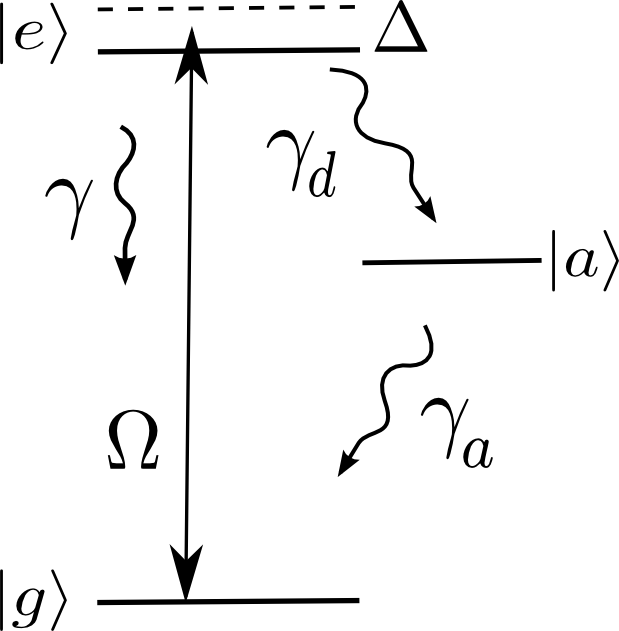
Figure 1: Scheme of the three-level atom showing laser excitation of the $|e\rangle-|g\rangle$ transition with Rabi frequency $\Omega$, detuning $\Delta$, and spontaneous decay rate $\gamma$, and spontaneous decay via the metastable state $|a\rangle$ at rates $\gamma_{d},\gamma_{a}$.

Model.— Our system, depicted in Fig. 1, consists of a three-level atom with one laser-driven transition with Rabi frequency $\Omega$, detuning $\Delta$ and decay rate $\gamma$, whose fluorescence is monitored. The excited state $|e\rangle$ also decays to a long-lived intermediate state $|a\rangle$ at the rate $\gamma_{d}$, and from this to the ground state at the rate $\gamma_{a}$.

The Markovian master equation in the frame rotating at the laser frequency is

$$\dot{\rho} = -i[\mathcal{H},\rho]+{\gamma}\mathcal{L}[\sigma_{ge}]\rho+{\gamma_{d}}\mathcal{L}[\sigma_{ae}]\rho+{\gamma_{a}}\mathcal{L}[\sigma_{ga}]\rho,$$ (1)

where $\mathcal{H}=\Delta\,\sigma_{eg}\sigma_{ge}+\Omega(\sigma_{eg}+\sigma_{ge})/2$ is the atom-laser Hamiltonian in the rotating wave approximation and $\mathcal{L}[\mathcal{O}]\rho\equiv\mathcal{O}\rho\mathcal{O}^{\dagger}-(\mathcal{O}^{\dagger}\mathcal{O}\rho+\rho\mathcal{O}^{\dagger}\mathcal{O})/2$ are spontaneous decay superoperators. The atomic operators $\sigma_{jk}=|j\rangle\langle k|$ obey $\sigma_{jk}\sigma_{lm}=\sigma_{jm}\delta_{kl}$.

Because of the pure spontaneous emission decay, the incoherent nature of the $|e\rangle-|a\rangle-|g\rangle$ channel decouples the equations for the coherences involving the $|a\rangle$ state from those of the laser driven $|e\rangle-|g\rangle$ transition CaRG16 ; EvKe02 . The Bloch equations of the effective two-level system can then be written in compact form as

$$\langle\dot{\mathbf{s}}(t)\rangle = \mathbf{M}\langle\mathbf{s}(t)\rangle+\mathbf{b},$$ (2)

$$\mathbf{s} \equiv \left(\sigma_{ge},\sigma_{eg},\sigma_{ee},\sigma_{gg}\right)^{T},$$ (3)

$$\mathbf{b} = (0,0,0,\gamma_{a})^{T},$$ (4)

$$\mathbf{M} = \left(\begin{array}[]{cccc}-i\Delta-\gamma_{+}/2&0&i\Omega/2&-i\Omega/2\\ 0&i\Delta-\gamma_{+}/2&-i\Omega/2&i\Omega/2\\ i\Omega/2&-i\Omega/2&-\gamma_{+}&0\\ -i\Omega/2&i\Omega/2&\gamma_{-}&-\gamma_{a}\end{array}\right),$$ (9)

$$\gamma_{+}=\gamma+\gamma_{d},\qquad\gamma_{-}=\gamma-\gamma_{a}.$$ (11)

Above, $\dot{\mathbf{s}}$ is the derivative of $\mathbf{s}$ with respect to time.

In general, the Bloch equations are solved numerically. However, accurate approximate analytical solutions in the resonant case, $\Delta=0$, in the regime (14) were obtained by two of us in CaRG16 . The populations and coherences show the typical short-term decay at the rate $3\gamma_{+}/4$ reminiscent of the 2LA dynamics and a long-term decay, at roughly $\gamma_{a}$, that signals shelving in the metastable state $|a\rangle$ PlKn98 .

The solutions in the steady state are

$$\langle\sigma_{eg}\rangle_{st} = \frac{i\Omega[\gamma_{+}+i2\Delta]}{(2+q)\Omega^{2}+\gamma_{+}^{2}+4\Delta^{2}},$$ (12a)

$$\langle\sigma_{gg}\rangle_{st} = \frac{\Omega^{2}+\gamma_{+}^{2}+4\Delta^{2}}{(2+q)\Omega^{2}+\gamma_{+}^{2}+4\Delta^{2}},$$ (12b)

$$\langle\sigma_{ee}\rangle_{st} = \frac{\Omega^{2}}{(2+q)\Omega^{2}+\gamma_{+}^{2}+4\Delta^{2}},$$ (12c)

$$\langle\sigma_{aa}\rangle_{st} = \frac{q\Omega^{2}}{(2+q)\Omega^{2}+\gamma_{+}^{2}+4\Delta^{2}},$$ (12d)

where

$$q = \gamma_{d}/\gamma_{a}.$$ (13)

and $\langle\sigma_{ge}\rangle_{st}=\langle\sigma_{eg}\rangle_{st}^{\ast}$.

This system features blinking, with long bright and dark periods in the fluorescence of the $|e\rangle-|g\rangle$ transition due to electron shelving in the metastable state $|a\rangle$, if the decay rates obey the relation

$$\gamma\gg\gamma_{d},\gamma_{a}.$$ (14)

A random telegraph model can be used to calculate the average length of the bright and dark periods EvKe02 ; PeKn88 . For this derivation the equation for the metastable state, $\dot{\rho}_{aa}=\gamma_{d}\rho_{ee}-\gamma_{a}\rho_{aa}$, is needed ($\rho_{jk}=\langle\sigma_{kj}\rangle$). During a bright period the state $|a\rangle$ is never occupied, $\rho_{aa}(t)=0$. The average bright time $T_{B}$ is defined as $T_{B}^{-1}=(\dot{\rho}_{aa})_{t\to\infty}$, where the limit means a time long enough for the two-level transition $|g\rangle-|e\rangle$ to reach the steady state, so $\rho_{ee}(\infty)\to(\rho_{ee}^{st})_{2LA}$. Thus, with $q=0$ and $\gamma_{+}\to\gamma$ in Eq. (12c), we have

$$T_{B}=\frac{2\Omega^{2}+\gamma^{2}+4\Delta^{2}}{\gamma_{d}\Omega^{2}}.$$ (15)

Similarly, the average dark time $T_{D}$ is defined as $T_{D}^{-1}=(\dot{\rho}_{aa})_{t\to\infty}$ but, during a dark period $\rho_{aa}(t)=1$ and $\rho_{ee}(t)=0$, hence

$$T_{D}=\gamma_{a}^{-1}.$$ (16)

The three-level scheme of Fig. 1 is a simplified theoretical representation of the complex energy level structure of an ${}^{171}\mathrm{Yb}^{+}$ ion under the driving configuration presented in BuTa00 . In this paper the stationary spectrum of ${}^{171}\mathrm{Yb}^{+}$ was measured where, in order to reduce the dark periods in the ion’s fluorescence, additional incoherent pumping from $|a\rangle$ to a fourth level (not shown) with faster decay to $|g\rangle$ was applied. Thus, $\gamma_{d}$ is considered an effective decay rate that includes such pumping.

Stationary Power Spectrum.— The stationary Wiener-Khintchine power spectrum is given by the Fourier transform of the field autocorrelation function FiTa17 ,

$$S(\omega) = \mathrm{Re}\int_{0}^{\infty}d\tau e^{-i\omega\tau}\langle\sigma_{eg}(0)\sigma_{ge}(\tau)\rangle_{st}.$$ (17)

By writing the atomic operators as the sum of a mean, $\langle\sigma_{jk}\rangle_{st}$, plus fluctuations, $\tilde{\Delta}\sigma_{jk}(t)$, that is, $\sigma_{jk}(t)=\langle\sigma_{jk}\rangle_{st}+\tilde{\Delta}\sigma_{jk}(t)$, we can separate the spectrum into a coherent part

$$S_{coh}(\omega) = |\langle\sigma_{eg}\rangle_{st}|^{2}\mathrm{Re}\int_{0}^{\infty}e^{-i\omega\tau}d\tau=\pi|\langle\sigma_{eg}\rangle_{st}|^{2}\delta(\omega),$$ (18)

$$= \frac{\pi\Omega^{2}(\gamma_{+}^{2}+4\Delta^{2})}{[(2+q)\Omega^{2}+\gamma_{+}^{2}+4\Delta^{2}]^{2}}\delta(\omega),$$

due to elastic scattering, and an incoherent part

$$S_{inc}(\omega) = \mathrm{Re}\int_{0}^{\infty}d\tau e^{-i\omega\tau}\langle\tilde{\Delta}\sigma_{eg}(0)\tilde{\Delta}\sigma_{ge}(\tau)\rangle_{st},$$ (19)

due to atomic fluctuations. For the strong transition of the V and $\Lambda$ 3LA’s, $S_{inc}(\omega)$ consists of a spectrum nearly identical to the 2LA Mollow one (peaks of width of the order of $\gamma$, a single one in the weak driving limit and a triplet in the strong excitation regime Mollow69 ) plus a narrow peak of nearly Lorentzian shape at the laser frequency due to the presence of electron shelving HePl95 ; GaKK95 .

Bühner and Tamm experimentally measured the narrow peak near the saturation regime by heterodyne detection BuTa00 . Later, Evers and Keitel EvKe02 studied the narrow peak in detail and found that it comes at the expense of the coherent peak of the 2LA spectrum. Noting in Eq. (18) that $q>0$, the coherent peak of the 3LA is smaller than that of the 2LA. Writing $\left(S_{coh}\right)_{NLA}=I_{NLA}\delta(\omega)$, for $N=2,3$, the relative intensity of the narrow inelastic peak is given by the difference in the size of the coherent peak of the two- and three-level atoms, $I_{np}=I_{2LA}-I_{3LA}$,

$$I_{np} = \left(|\langle\sigma_{eg}\rangle_{st}|^{2}\right)_{2LA}-\left(|\langle\sigma_{eg}\rangle_{st}|^{2}\right)_{3LA}$$

$$= \frac{\Omega^{4}[(2+q)\gamma^{2}-2\gamma_{+}^{2}+4\Delta^{2}q]}{[2\Omega^{2}+\gamma^{2}+4\Delta^{2}]^{2}[(2+q)\Omega^{2}+\gamma_{+}^{2}+4\Delta^{2}]^{2}}.$$

The narrow peak becomes smaller for increasing Rabi frequencies, but increasing detuning enhances the peak if the Rabi frequency is increased EvKe02 ; this peak is the largest for a detuning $\Delta_{max}^{2}=\left[(q-2)\Omega^{2}-2\gamma^{2}\right]/8$. The width of the narrow peak is accurately given by HePl95 ; EvKe02

$$\Gamma_{np} = T_{D}^{-1}+T_{B}^{-1}$$ (21)

$$= \gamma_{a}\left[1+\frac{q\Omega^{2}}{2\Omega^{2}+\gamma^{2}+4\Delta^{2}}\right].$$

An analytic formula for the full stationary spectrum on resonance in the regime (14) has been given in CaRG16 .

Time-Dependent Spectrum.— We calculate time-dependent spectra (TDS) using the physical spectrum of Eberly and Wódkiewicz EbWo77

$$S(D,t,\Gamma) = \Gamma\int_{t_{0}}^{t}dt_{1}\int_{t_{0}}^{t}dt_{2}\,\,e^{-(\Gamma/2-iD)(t-t_{1})}$$ (22)

$$\times e^{-(\Gamma/2+iD)(t-t_{2})}\langle\sigma_{eg}(t_{1})\sigma_{ge}(t_{2})\rangle,$$

where $D=\omega-\omega_{l}$ is the detuning of the laser frequency $\omega_{l}$ from the filter’s frequency $\omega$, and $\Gamma$ is the filter’s bandwidth. Admittedly, the calculation of TDS is not a simple task, and more often than not a numerical solution is required. Some authors often wish to avoid the filter effects and resort to simpler, yet probably defective, approaches EbWo77 ; FiTa17 . The inclusion of the filter ensures that the time-energy uncertainty is properly accounted for in theoretical calculations. An additional benefit of filtering is that it can enhance important features and the signal to noise ratio in the measured TDS of weak signals.

For computation purposes it is convenient to rewrite the double integral in terms of integrals for $t_{2}$ and $\tau=t_{1}-t_{2}$ EbKW80 ; making $t_{0}=0$ we have

$$S(\omega,t,\Gamma) = 2\Gamma\mathrm{Re}\Big{[}\int_{0}^{t}dt_{2}e^{-\Gamma(t-t_{2})}\int_{0}^{t-t_{2}}d\tau\,e^{(\Gamma/2-iD)\tau}$$ (23)

$$\times\langle\sigma_{eg}(t_{2}+\tau)\sigma_{ge}(t_{2})\rangle\Big{]}.$$

To solve for the two-time correlations we apply the quantum regression formula Carm02 to Eq. (2) obtaining

$$\partial_{\tau}\langle\mathbf{u}(t_{2},\tau)\rangle = \mathbf{M}\langle\mathbf{u}(t_{2},\tau)\rangle+\mathbf{c}(t_{2}),$$ (24)

where

$$\mathbf{u}(t_{2},\tau) = \big{[}\sigma_{ge}(t_{2}+\tau)\sigma_{ge}(t_{2}),\sigma_{eg}(t_{2}+\tau)\sigma_{ge}(t_{2}),$$

$$\sigma_{ee}(t_{2}+\tau)\sigma_{ge}(t_{2}),\sigma_{gg}(t_{2}+\tau)\sigma_{ge}(t_{2})\big{]}^{T},$$

$$\mathbf{c}(t_{2}) = (0,0,0,\gamma_{a}\langle\sigma_{ge}(t_{2})\rangle)^{T},$$

which we solve numerically with initial condition $\mathbf{u}(t_{2},0)=\left(0,\sigma_{ee}(t_{2}),0,\sigma_{ge}(t_{2})\right)^{T}$. The number of parameters in our system makes it very difficult to obtain analytical expresions for the TDS.

Figures 2-4 show our results for the TDS of our blinking system. Figure 2 displays the spectra in the excitation regime near saturation, $\Omega=\gamma_{+}/4$. A narrow peak develops for long times, $\gamma t\gg 1$, above a background given by the usual broad peak of width $\sim\gamma$ formed on a shorter time scale of several lifetimes, $\gamma^{-1}$.

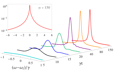
Figure 2: Time-dependent spectra for moderate laser field strength, $\Omega=\gamma_{+}/4=0.2625\gamma$, $\gamma_{d}=0.05\gamma$ and $\gamma_{a}=0.015\gamma$. The filter’s bandwidth is $\Gamma=0.1\gamma$. The inset shows the spectrum at $\gamma t=150$ in semi-log scale and wider frequency range to reveal the broad component.

To better appreciate the different time scales for the appearance of the spectral components we show the TDS in the strong field regime, $\Omega=3.5\gamma$. In Fig. 3, while the triplet is well developed for times $\gamma t\sim 10$ the narrow peak arises at about $\gamma t\sim 20$. As expected from the stationary spectrum, the narrow peak in the strong field regime is smaller than in the saturation regime EvKe02 ; CaRG16 . Hence, as suggested in EvKe02 , some detuning notably enhances the narrow peak against the spectral background of the Mollow triplet, as shown in Fig. 4. A slight asymmetry occurs in the detuned case that vanishes in the long time limit EbKW80 ; in this case one of the sidebands is closer to the atomic resonance and is larger than the other EbKW80 , while the asymmetry in the center of the spectrum gets smaller (see inset). More pronounced spectral asymmetries are found, for example, in detuned pulsed laser resonance fluorescence GuMH18 .

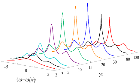
Figure 3: Same as Fig. 2 but for strong driving, $\Omega=3.5\gamma$.

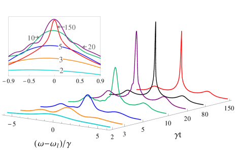
Figure 4: TDS for strong field, $\Omega=3.5\gamma$, but detuning $\Delta=1$. The other parameters as in Fig. 2. The inset shows the diminishing asymmetry of the center of the spectrum for increasing time.

It is important to note that while the narrow peak develops much later than the Mollow spectrum, it does actually emerge, if not stabilize, well before an average dark time $T_{D}$ has passed. The presence of dark periods in the fluorescence is felt soon in the ensemble’s evolution: in some realizations of the ensemble the dark period may occur before the bright one. From Eqs. (15) and (16) it is seen that the average bright time depends on both laser and atomic parameters, while the average dark period depends only on the effective lifetime $\gamma_{a}^{-1}$ of the metastable state $|a\rangle$. In the TDS sequences of Figs. 2 – 4, $\gamma T_{D}\simeq 67$, and $\gamma T_{B}\simeq 330,42$, and 48, respectively. They reveal the time scale of the dark and bright periods in the ensemble evolution.

We have to discuss also effects of the filter on the EW time-dependent spectrum. First, it could be argued that the observed narrow peak is the filter-broadened coherent spectral component. This is not the case because the delta peak is a steady state feature of the spectrum FiTa17 ; it should not appear in a TDS, however long is the finite observation time. What we undoubtedly see is the incoherent narrow peak produced by random interruptions in the fluorescence of the strong transition $|g\rangle-|e\rangle$ caused by the atom’s excursions into the weak transition channel $|e\rangle\to|a\rangle\to|g\rangle$ HePl95 . Moreover, the narrow peak grows at the expense of the coherent peak EvKe02 : its intensity is the difference among the intensities of the coherent peak of the two- and three-level systems, Eq. (Time-dependent spectra of a three-level atom in the presence of electron shelving).

Another issue is the choice of filter bandwidth $\Gamma$. On one hand, it must be able to resolve the different spectral components, therefore $\Gamma$ should be a fraction of the width, $\sim\gamma$, of the Mollow spectral peaks. On the other, $\Gamma$ cannot be infinitely small, as is assumed for the stationary spectrum EbWo77 . The filter bandwidth in our plots, $\Gamma=0.1\gamma$, was chosen to focus on the narrow peak: for $\Gamma>\Gamma_{np}$ the filter sets the observed width of the narrow peak.

The filter bandwidth also has dynamical consequences due to the time-energy uncertainty; the filter has to saturate in order to finish its transient effect and begin to produce stable spectra. This occurs after a time $\Gamma t>1$. Hence, a narrow filter $\Gamma<\gamma$ causes a delay in the stabilization of the fast-forming Mollow-like spectrum EbKW80 , while the narrow peak stabilizes soon since $\Gamma<\Gamma_{np}$. The transient effects on a spectrum are therefore felt for very long times, as seen in the temporary reduction of the spectra of Figs. 3 and 4. The different time scales due to atomic and filter parameters make it very difficult to fully assess the TDS analytically.

Finally, we have used a density-operator-based approach, for which the TDS is the statistical average of infinitely many realizations. However, while the individual records of bright and dark periods are buried in the ensemble average, the impact of the latter on the TDS is evident in the emergence of the incoherent narrow peak.

Conclusions.— We have investigated the time-dependent spectrum of intermittent resonance fluorescence and found that the narrow incoherent peak due to electron shelving emerges and stabilizes much later than the Mollow spectrum. We trust that an experimental observation of blinking resonance fluorescence TDS is within reach. TDS of two-level atom resonance fluorescence have been observed GoMo87 and measurements of shelving fluorescence have reached the accuracy required for applications such as precision measurements of fundamental constants and optical ion clocks GNJ+14 ; HLT+14 . We think that even for nonergodic blinking such as that of quantum dots or molecules StHB09 , whose TDS have been studied in LeBa15 , the Eberly-Wódkiewicz physical spectrum would be of great benefit. The observation and interpretation of TDS could help to describe the dynamics of other systems with separate time scales such as super- and sub-radiance vLFL+13 and entanglement HoFi10 in collective atomic dynamics.

Acknowledgments.— R. R.-A. wishes to thank CONACyT, Mexico for scholarship 379732. H.M.C.-B. thanks Prof. J. Récamier for hospitality at ICF-UNAM.

References

- (1) W. Nagourney, J. Sandberg, and H. Dehmelt, Phys. Rev. Lett. 56, 2797 (1986).
- (2) Th. Sauter, W. Neuhauser, R. Blatt, and P. E. Toschek, Phys. Rev. Lett. 57, 1696 (1986).
- (3) J. C. Bergquist, R. G. Hulet, W. M. Itano, and D. J. Wineland, Phys. Rev. Lett. 57, 1699 (1986).
- (4) M. B. Plenio and P. L. Knight, Rev. Mod. Phys. 70, 101 (1998).
- (5) Z. K. Minev et al, arXiv 1803.00545v1.
- (6) M. Merz and A. Schenzle, Appl. Phys. B 50, 115 (1990).
- (7) H. M. Castro-Beltrán, R. Román-Ancheyta, and L. Gutiérrez, Phys. Rev. A 93, 033801 (2016).
- (8) G. C. Hegerfeldt and M. B. Plenio, Phys. Rev. A 52, 3333 (1995).
- (9) B. M. Garraway, M. S. Kim, and P. L. Knight, Opt. Commun. 117, 560 (1995).
- (10) B. R. Mollow, Phys. Rev. 188, 1969 (1969).
- (11) V. Bühner and Chr. Tamm, Phys. Rev. A 61, 061801 (2000).
- (12) J. Evers and Ch. H. Keitel, Phys. Rev. A 65, 033813 (2002).
- (13) G. C. Hegerfeldt and M. B. Plenio, Phys. Rev. A 53, 1164 (1996).
- (14) J. H. Eberly and K. Wódkiewicz, J. Opt. Soc. Am. 67, 1252 (1977).
- (15) J. H. Eberly, C. V. Kunasz, and K. Wódkiewicz, J. Phys. B: Atom. Molec. Phys. 13, 217 (1980).
- (16) X. Y. Huang, R. Tanaś, and J. H. Eberly, Phys. Rev. A 26, 892 (1982).
- (17) J. E. Golub and T. W. Mossberg, Phys. Rev. Lett. 59, 2149 (1987).
- (18) A. S. Jayarao, S. V. Lawande, and R. D’Souza, Phys. Rev. A 39, 3464 (1989).
- (19) J. J. Sanchez-Mondragon, N. B. Narozhny, and J. H. Eberly, Phys. Rev. Lett. 51, 550 (1983); ibid 51, 1925 (1983).
- (20) H. M. Castro-Beltran, J. J. Sanchez-Mondragon, and S. M. Chumakov, Phys. Rev. A 53, 4420 (1996).
- (21) E. del Valle, A. Gonzalez-Tudela, F. P. Laussy, C. Tejedor, and M. J. Hartmann, Phys. Rev. Lett. 109, 183601 (2012).
- (22) A. W. Glaetzle, K. Hammerer, A. J. Daley, R. Blatt, and P. Zoller, Opt. Commun. 283, 758 (2010).
- (23) I. M. Mirza, J. Opt. Soc. Am. B 32, 1604 (2015).
- (24) L. Horvath and Z. Ficek, J. Phys. B: At. Mol. Opt. Phys. 43, 125506 (2010).
- (25) D. T. Pegg and P. L. Knight, Phys. Rev. A 37, 4303 (1988); D. T. Pegg and P. L. Knight, J. Phys. D: Appl. Phys. 21, S128 (1988).
- (26) Z. Ficek and R. Tanaś, Quantum-Limit Spectroscopy (Springer, New York, 2017).
- (27) H. J. Carmichael, Statistical Methods in Quantum Optics 1: Master Equations and Fokker-Planck Equations (Springer-Verlag, Berlin, 2002).
- (28) C. Gustin, R. Manson, and S. Hughes, Opt. Lett. 43, 779 (2018).
- (29) R. M. Godun, P. B. R. Nisbet-Jones, J. M. Jones, S. A. King, L. A. M. Johnson, H. S. Margolis, K. Szymaniec, S. N. Lea, K. Bongs, and P. Gill, Phys. Rev. Lett. 113, 210801 (2014).
- (30) N. Huntemann, B. Lipphardt, Chr. Tamm, V. Gerginov, S. Weyers, and E. Peik, Phys. Rev. Lett. 113, 210802 (2014).
- (31) F. D. Stefani, J. P. Hoogenboom, and E. Barkai, Phys. Today 62(2), 34 (2009).
- (32) N. Leibovich and E. Barkai, Phys. Rev. Lett. 115, 080602 (2015).
- (33) A. F. van Loo, A. Fedorov, K. Lalumière, B. C. Sanders, A. Blais, and A. Wallraff, Science 342, 1494 (2013).