Stabilizing quantum coherence against pure dephasing in the presence of quantum coherent feedback at finite temperature

Abstract

A general formalism to describe the dynamics of quantum emitters in structured reservoirs is introduced. As an application, we investigate the optical coherence of an atom-like emitter diagonally coupled via a link-boson to a structured bosonic reservoir and obtain unconventional dephasing dynamics due to non-Markovian quantum coherent feedback for different temperatures. For a two-level emitter embedded in a phonon cavity, preservation of finite coherence is predicted up to room temperature.

March 5, 2024

I Introduction

Few-level quantum systems such as atoms, molecules, and their artificial counterparts in solid state structures are envisioned as fundamental building blocks of quantum communication, encryption and computation Nielsen and Chuang (2010); Gardiner and Zoller (2015); Zubairy and Scully (1997); Zoller et al. (2005). Quantum dots in solid state systems are approximated as few-level, or in the ideal case, two-level emitters (TLE), which is similar to the way atoms are handled in quantum optics Walls and Milburn (2008). The interaction of these dots with the collective excitations of the surrounding bulk material - especially acoustic phonons - are perceived as the main threat to coherence in these systems. These decoherence processes also hinder the efficient functioning of quantum information processing on such platforms May and Kühn (2008); Bimberg (2008); Nazir and McCutcheon (2016); Iles-Smith et al. (2017).

Optical excitation of these quantum dots restructures the local electron configuration, and induces lattice vibration around the equilibrium positions of the atomic cores in the bulk. While the system equilibrates, the generated phonons induce a wide range of phenomena such as the damping of Rabi oscillations Förstner et al. (2003, 2003), cavity-feeding Roy-Choudhury and Hughes (2015), striking photon-phonon coupling Roy and Hughes (2011); Harsij et al. (2012), incoherent excitation of the emitter Hughes and Carmichael (2013); Weiler et al. (2012); Wigger et al. (2014), and phonon-assisted quantum interferences Carmele et al. (2013); Wilson-Rae and Imamoğlu (2002). Thus, in comparison to isolated atomic systems, solid state systems are generally considered to have larger dephasing and damping rates, most of which could be overcome only by cooling the system to very low temperatures. However, phonon emission is still a source of decoherence even at 0 K.

Due to the interaction with the solid state environment (via, e.g., acoustic phonons), these processes cannot be completely eliminated, but the idea of controlling them has motivated theoretical investigations to turn this drawback into a useful and essential feature. In recent proposals a dissipative interaction is used to induce phonon-lasing Droenner et al. (2017), ground-state cooling Martin et al. (2004); Jaehne et al. (2008), or even stabilization of the dynamics Bounouar et al. (2015); Carmele et al. (2013); Glässl et al. (2012) in the strong coupling regime. Nevertheless, for efficient reservoir engineering, a more general theoretical framework is needed to understand, describe, and control a wide variety of different systems and structured reservoirs at finite temperatures.

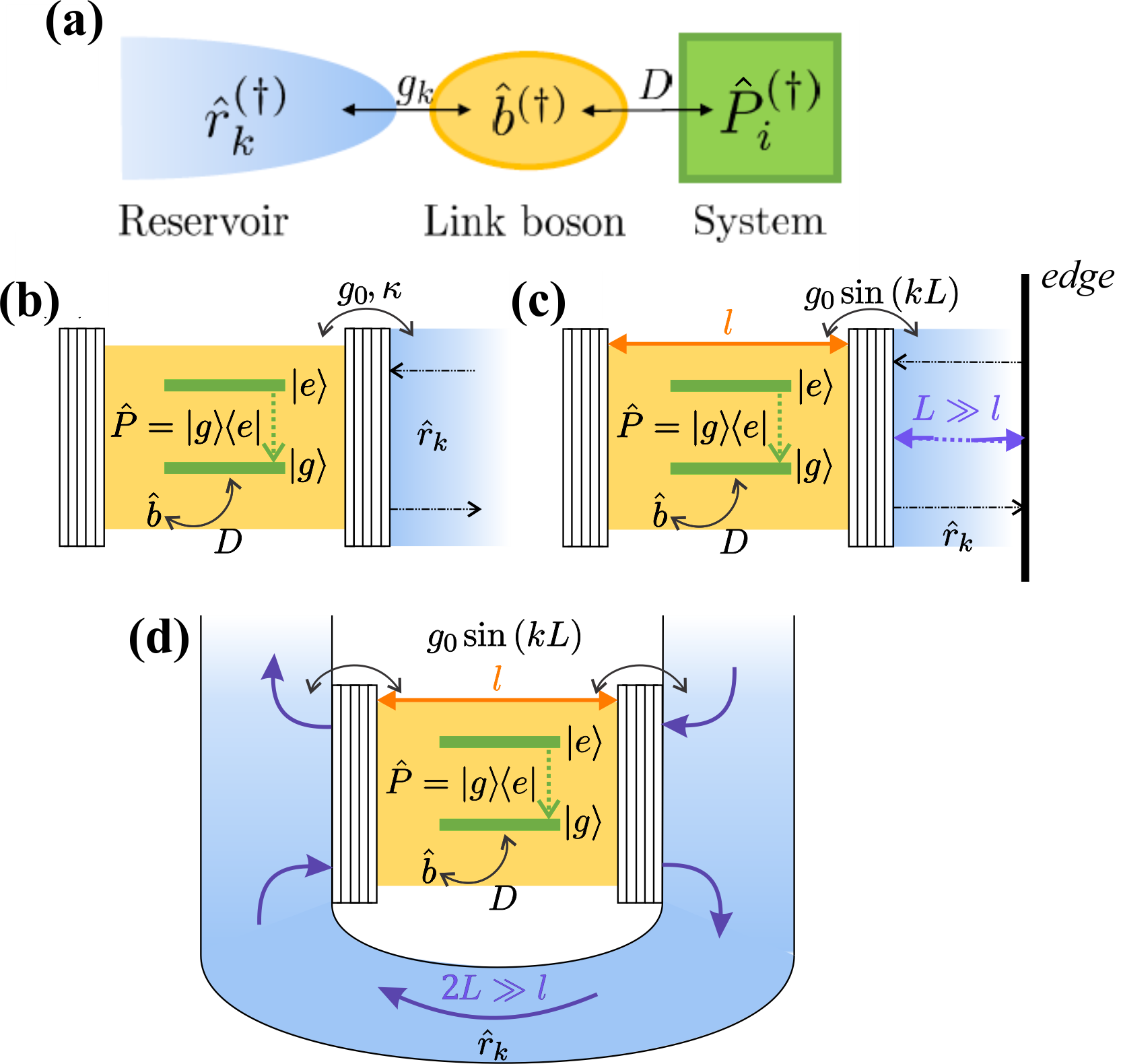
Figure 1: (a) Schematics of potential setups to consider. An example where this approach can be applied is a quantum emitter coupled to a single-mode phonon cavity, which is embedded in a waveguide without edge (b), and with a perfectly reflecting edge (c). An alternative, unidirectional realization for the feedback case with chiral coupling to the waveguide can also be considered, where $2L$ is the length of the feedback loop (d).

In this Paper, we propose a model where a two-level emitter (TLE) is coupled to a dissipative boson, such as an optical phonon Hameau et al. (1999); Krauss and Wise (1997); Carmele et al. (2010) or an acoustic cavity mode Fainstein et al. (2013); Lanzillotti-Kimura et al. (2015); Trigo et al. (2002); Kabuss et al. (2012). In practice, such a dissipative, single bosonic mode can be realized by phonon-confinement in layered structures Trigo et al. (2002); Pascual Winter et al. (2005); Soykal et al. (2011); Anguiano et al. (2017) or photonic-phononic crystals Fainstein et al. (2013); Lanzillotti-Kimura et al. (2015). We address this boson as link boson since it provides a link between the system and the bosonic reservoir. The dynamics of the link boson can be controlled via its initial state and interaction with the reservoir (Fig. 1(a)). This reservoir of the link boson (LB) has typically infinite degrees of freedom but can be spectrally unstructured, as in Fig. 1(b), or structured by, e.g., a perfectly reflecting edge (Fig. 1(c)) or an imposed chiral coupling (Fig. 1(d)). A reservoir-structuring as shown in Fig. 1(c) can be realized by phononic Bragg mirrors Trigo et al. (2002); Pascual Winter et al. (2005); Soykal et al. (2011); Anguiano et al. (2017); Fainstein et al. (2013); Lanzillotti-Kimura et al. (2015). This way, the infinite degrees of freedom of the solid state reservoir amount either to enhanced or suppressed dephasing of the TLE Pirkkalainen et al. (2013); Carmele et al. (2013) and may even introduce, e.g., time-delayed feedback for the system’s dynamics Faulstich et al. (2018).

The other side of the coin is that there are unique and yet not understood non-Markovian effects present in solid state systems intrinsically Cassabois and Ferreira (2008); Moody et al. (2012); Thoma et al. (2016); Liu et al. (2018). The introduction of a link boson - with its extra degrees of freedom - facilitates the development of an effective model of these non-trivial dephasing dynamics. One important feature of our introduced method in that respect is the ability to separately control the Markovian ($g_{0}$) and non-Markovian ($D$ and $L$) characteristics.

The interaction between acoustic phonons and the TLE can be formulated as a level-shifting, pure-dephasing-type interaction Bimberg (2008); Nazir and McCutcheon (2016), where an additional Ohmic spectral density is considered for the continuum of phonon modes that introduces non-Markovian correlations Leggett et al. (1987); Besombes et al. (2001); Favero et al. (2003). This model, the independent boson model, accurately describes the dephasing dynamics of the emitter in the linear regime. However, due to the absence of excitation exchange, it is limited to unilateral phase-destroying processes without the build-up of quantum entanglement between emitter and reservoir Petruccione et al. (2007); Nazir and McCutcheon (2016); Krummheuer et al. (2002); Pazy (2002); May and Kühn (2008); Agarwal (2012). Here, by connecting the emitter via a LB to the solid state reservoir and allowing for excitation transfer between them, we demonstrate how one can overcome this limitation. The considered exchange of excitations introduces quantum interference into the system dynamics, enables reservoir-engineered quantum coherence, and forms a robust recipe for quantum state preparation Ramos et al. (2013); Law and Eberly (1996).

Focusing only on boson-emitter interactions, the investigated model in the present work can be applied in diverse settings, ranging from acoustic phonons and quantum dots to a wide range of other setups, especially in the context of circuit QED. Micro- and nanomechanical resonators coupled to Nitrogen-vacancy centres Rabl et al. (2009); Arcizet et al. (2011), Cooper boxes Armour et al. (2002); Irish and Schwab (2003); Martin et al. (2004); Jaehne et al. (2008); LaHaye et al. (2009); Stadler et al. (2017), Josephson junctions and SQUIDs Xue et al. (2007); Etaki et al. (2008); Khosla et al. (2018) are perfect platforms for testing fundamental quantum mechanics as well as quantum non-demolition measurement of the TLE Johnson et al. (2010); Reiserer et al. (2013). Also, in optical lattices, recent experiments show strong control over single vibrational modes in ion traps with generalized pure dephasing coupling Lemmer et al. (2018). A straightforward extension of these systems are when the quantum emitter is located on the surface of the mechanical resonator interacting with the vibrational mode via a strain-mediated coupling Wilson-Rae et al. (2004); Yeo et al. (2013); Munsch et al. (2017); Ramos et al. (2013).

In the following, we demonstrate that the introduction of a link boson allows a simple yet powerful analytical solution for a wide range of dynamics unattainable within the typical independent boson model Krummheuer et al. (2002); May and Kühn (2008); Agarwal (2012). The presented model demonstrates the link between the two kinds of non-Markovianity, i.e., the one that is observed as naturally appearing in solid state systems and the one that is the topical case of artificially structured reservoirs in quantum optics. An example of such a structured reservoir that we consider is a coherent, feedback-type, reservoir-LB interaction, which can be used to steer the dynamics of the TLE with the goal of coherence preservation. Moreover, even though there are numerical methods that in principle are capable of characterizing the effect of quantum coherent feedback at a finite temperature Pichler and Zoller (2016); Whalen and Carmichael (2016), to our knowledge, this is the first work to report on the exact influence of this effect on the amount of recovered coherence.

II Theoretical Model

For generality, our model considers an arbitrary set of system operators $\hat{P}^{(\dagger)}_{i}$ that can be coupled to a single bosonic mode with annihilation (creation) operator $\hat{b}^{(\dagger)}$. This link boson (LB) couples the system (S) to another bosonic reservoir described by operators $\hat{r}_{k}^{(\dagger)}$; see Fig.1(a). Thus, in its most general form, the model assumes the following Hamiltonian,

$$\hat{H}= \ \hat{H}_{S}+\hat{H}_{R}+\hat{H}_{LB}\left(\hat{b},\hat{b}^{\dagger},\hat{P}^{\phantom{\dagger}}_{i},\hat{P}_{i}^{\dagger}\right),$$ (1)

where $\hat{H}_{S}$ describes the free evolution of the system operators $\hat{P}^{\dagger}_{i}$, i.e., $\hat{H}_{S}=\sum_{i}\hbar\omega_{i}\hat{P}^{\dagger}_{i}\hat{P}_{i}$. The LB interacts with the bosonic reservoir via $\hat{H}_{R}$,

$$\hat{H}_{R}/\hbar= \omega_{0}\hat{b}^{\dagger}\hat{b}\ +\int\left[\omega_{k}\hat{r}^{\dagger}_{k}\hat{r}_{k}+g_{k}(\hat{r}^{\dagger}_{k}\hat{b}+\hat{b}^{\dagger}\hat{r}_{k})\right]dk,$$ (2)

where $k$ labels the lowering (raising) operator for a reservoir mode with wave number $k$, and $g_{k}$ describes the $k$-dependent interaction strength between the two bosonic fields. The system and the LB interact via the interaction Hamiltonian $\hat{H}_{LB}\left(\hat{b},\hat{b}^{\dagger},\hat{P}^{\phantom{\dagger}}_{i},\hat{P}_{i}^{\dagger}\right)$ with coupling strength $D_{i}$ (see Fig.1(a)), which will be specified later.

The effective action of the reservoir $\{\hat{r}_{k}^{\phantom{\dagger}},\hat{r}_{k}^{\dagger}\}$ on the LB is given by the solution of the LB-reservoir dynamics, as described by $\hat{H}_{R}$ in Eq. (2). Using Heisenberg equations of motion, the LB-dynamics can be represented with a linear map,

$$\hat{b}(t) =F(t)\hat{b}(0)+\int G_{k}(t)\hat{r}_{k}(0)dk,$$ (3)

where $F(t)$ and $G_{k}(t)$ are $c$-number functions satisfying $[\hat{b}(t),\hat{b}^{\dagger}(t)]=1$ at all times. We provide in the following two examples for the LB-reservoir interaction.

Case (i): a dissipative, Markovian, irreversible interaction of the LB with its reservoir $(g_{k}=g_{0})$. A typical example is given in Fig. 1(b), where a single two-level system couples to a single mode of a photonic/phononic nanocavity $b^{(\dagger)}$. The Markovian interaction leads to a dissipative link boson dynamics and to the propagators

$$F_{d}(t) =e^{-(i\omega_{0}+\kappa)t},$$ (4)

$$G^{d}_{k}(t) =-ig_{0}\int_{0}^{t}e^{-(i\omega_{0}+\kappa)(t-{t^{\prime}})-i\omega_{k}{t^{\prime}}}d{t^{\prime}},$$ (5)

where $\kappa=\pi g_{0}^{2}/(2c)$ is the decay rate of the LB into the continuum of modes of the reservoir. This case is well documented in the literature Zubairy and Scully (1997); Gardiner and Zoller (2015); May and Kühn (2008); Weiss (2012); Huelga et al. (2012).

On the other hand, in case (ii) we consider a $k$-dependent coupling $\left(g_{k}\right)$ structuring the reservoir mode. This is realized by a half-open cavity scheme for the link boson and a distant reflector in the environment, as shown in Fig. 1(c). This reservoir coupling produces a coherent, time-delayed feedback to the LB $(g_{k}=g_{0}\sin[ck\tau/2])$, where $\tau=2L/c$ is the roundtrip time and $c$ is determined by the dispersion relation valid in the reservoir Weiss (2012); Breuer and Petruccione (2002). An equivalent representation of this feedback scheme is shown in Fig. 1(d). In this case a chiral coupling to the waveguide imposes unidirectional flow of information back to the system. The roundtrip time now is translated into the length of the feedback loop, $2L$.

Solving exactly the reservoir-LB dynamics leads to the following c-number functions $F,G$ (see Appendix A for a detailed derivation),

$$F_{fb}(t) =\sum_{m=0}^{\infty}\frac{\kappa^{m}}{m!}e^{-B(t-m\tau)}(t-m\tau)^{m}\theta(t-m\tau),$$ (6)

$$G_{k}^{fb}(t) =\sum_{m=0}^{\infty}\frac{-ig_{k}\kappa^{m}\theta(t-m\tau)}{(A_{k}+B)^{m+1}}\left[e^{A_{k}(t-m\tau)}-\right.$$ (7)

$$\quad-\left.e^{-B(t-m\tau)}\sum_{n=0}^{m}\frac{1}{n!}(A_{k}+B)^{n}(t-m\tau)^{n}\right],$$

where $\kappa$ is defined as before and the coefficients as $A_{k}=-i\omega_{k}$ and $B=i\omega_{0}+\kappa$. The expressions above include non-trivial feedback quantities depending on the previous roundtrips (integer multiples of $\tau$) of the fields $b$ and $r_{k}$. These terms enable some interesting quantum interference phenomena, such as coherence stabilization, and give access to the reservoir dynamics Kabuss et al. (2015); Dorner and Zoller (2002); Kabuss et al. (2016); Guimond et al. (2017).

II.1 General interaction

Let us consider an interaction Hamiltonian, $\hat{H}_{LB}$, involving arbitrary system and link boson operators. The main objective of the applied method is to calculate the time-evolution of a given system operator $\hat{P}$ analytically for different initial conditions of both the system and the reservoir, as well as for different couplings between the two.

Since the effect of the surrounding reservoir dynamics is fully incorporated in the LB’s time trace, we can evaluate the Liouville-von Neumann equation explicitly in the interaction picture,

$$-i\hbar\frac{d}{dt}\hat{\rho}_{I}(t)=[\hat{H}_{LB}(t),\hat{\rho}_{I}(t)],$$

and from Eq.(1,2),

$$\hat{H}_{LB}(t) =\hat{U}(t)\hat{H}\hat{U}^{\dagger}(t)-i\hbar\hat{U}(t)\dot{\hat{U}}^{\dagger}(t),$$

$$\hat{U}(t) =\exp{\left(i(\hat{H}_{S}+\hat{H}_{R})t\right)},$$

since the system operators commute with the reservoir. Thus note, the system-LB interaction becomes time-dependent, and in the time-dependence the full reservoir interaction is present (see the derivation in Appendix A).

For a quadratic system Hamiltonian $\hat{H}_{S}$ with only real eigenvalues, there can be found a set of system operators $\{\hat{\Pi}_{i}\}$, the normal modes of the system, for which the time-dependence has the following form,

$$\hat{\Pi}_{i}(t)=e^{-i\omega_{i}t}\hat{\Pi}_{i}(0).$$ (8)

Any given system operator $\hat{P}$ can be constructed from these operators as

$$\hat{P}(t)=\sum_{i}\left[\alpha_{i}\hat{\Pi}_{i}(t)+\beta_{i}\hat{\Pi}^{\dagger}_{i}(t)\right],$$ (9)

$$\sum_{i}\left(|\alpha_{i}|^{2}+|\beta_{i}|^{2}\right)=1.$$

If we want to interpret the normal modes as quasiparticles with bosonic or fermionic commutation relations, the conditions

$$|\alpha_{i}|^{2}\pm|\beta_{i}|^{2}=1$$

also apply, with "$-$" corresponding to bosons and "$+$" to fermions.

Using the Liouville-von Neumann equation, for each of the normal mode operators we can prescribe the following equation

$$\frac{d\hat{\rho}_{I}}{dt}\hat{\Pi}_{i}(t)=-\frac{i}{\hbar}\left[\hat{H}_{LB},\hat{\rho}_{I}\right]\hat{\Pi}_{i}(t).$$ (10)

If the commutation relationship between the interaction Hamiltonian and $\hat{\Pi}_{i}(0)$ can be written as

$$\left[\hat{H}_{LB}(t),\hat{\Pi}_{i}(0)\right]=\hat{C}_{i}(t),$$ (11)

and using the time-evolution of $\hat{\Pi}_{i}$, Eq. (8), the following equation of motion can be obtained,

$$\text{Tr}\left(\frac{d\hat{\rho}_{\Pi_{i}}(t)}{dt}\right) =-\frac{i}{\hbar}Tr\left\{\left[\hat{H}_{LB},\hat{\rho}_{\Pi_{i}}(t)\right]-\hat{\rho}_{I}\hat{C}_{i}(t)\right\}=$$

$$=\frac{i}{\hbar}Tr\left\{\left[\hat{\Pi}_{i}^{-1}(0)\hat{C}_{i}(t)\right]\hat{\rho}_{\Pi_{i}}(t)\right\}$$ (12)

$$\hat{\rho}_{\Pi_{i}}(t) =\hat{\rho}_{I}(t)\hat{\Pi}_{i}(0),$$ (13)

which, due to the linear property of the trace, translates into

$$\frac{d}{dt}\boldsymbol{\big{\langle}}\hat{\Pi}_{i}(t)\boldsymbol{\big{\rangle}} =-\frac{i}{\hbar}\boldsymbol{\big{\langle}}\hat{\mathcal{D}}_{i}(t)\hat{\Pi}_{i}(t)\boldsymbol{\big{\rangle}},$$ (14)

$$\hat{\mathcal{D}}_{i}(t) =-\hat{\Pi}_{i}^{-1}(0)\hat{C}_{i}(t).$$ (15)

A stroboscopic solution for this equation for short enough time steps gives

$$\boldsymbol{\big{\langle}}\hat{\Pi}_{i}(t+\Delta t)\boldsymbol{\big{\rangle}} =\left\langle\left(1-\frac{i}{\hbar}\hat{\mathcal{D}}_{i}(t)\Delta t\right)\hat{\Pi}_{i}(t)\right\rangle\approx$$

$$\approx\left\langle e^{-\frac{i}{\hbar}\hat{\mathcal{D}}_{i}(t)\Delta t}e^{-\frac{i}{\hbar}\hat{\mathcal{D}}_{i}(t-\Delta t)\Delta t}\hat{\Pi}_{i}(t-\Delta t)\right\rangle,$$

which, by applying the Baker-Campbell-Hausdorff formula, turns into

$$\boldsymbol{\big{\langle}}\hat{\Pi}_{i}(t)\boldsymbol{\big{\rangle}}=\left\langle\exp{\left[-\frac{i}{\hbar}\int_{0}^{t}\hat{\mathcal{D}}_{i}(t_{1})dt_{1}\right]}\cdot\right.$$ (16)

$$\hskip 17.07182pt\cdot\left.\exp{\left[-\frac{1}{2\hbar^{2}}\int_{0}^{t}\int_{0}^{t_{1}}\left[\hat{\mathcal{D}}_{i}(t_{1}),\hat{\mathcal{D}}_{i}(t_{2})\right]dt_{2}dt_{1}\right]}\hat{\Pi}_{i}(0)\right\rangle.$$

The time evolution of the expectation value of the original system operator $\hat{P}(t)$ can be constructed from these expectation values by using (9).

II.2 TLE-phonon interaction

As we saw in the previous subsection, the model is applicable to a wide range of system-LB interactions. To provide an example, we consider the interaction between an optically excited spin/two-level emitter and a single-phonon mode Feynman and Vernon Jr (2000). This specific example (see Figs. 1(b-d)) is of great importance, as it describes the loss of coherence in quantum systems enforced by level-shifts of the emitter Calarco et al. (2003); Borri et al. (2005); Krügel et al. (2005) or between quantum emission processes influencing the indistinguishability of photons Thoma et al. (2016); Kaer et al. (2013); Unsleber et al. (2015),

$$\hat{H}_{LB}(t)=\hbar D[\hat{b}(t)+\hat{b}^{\dagger}(t)]\hat{P}^{\dagger}(t)\hat{P}(t),$$ (17)

where $\hat{P}=\left|g\right\rangle\left\langle e\right|$ is the lowering operator of the TLE. Note, that this model implies the pure dephasing limit, where the level-spacing of the TLE $\left(\hbar\omega_{i}=\hbar\omega_{eg}\right)$ is much greater than the energy of the LB $\left(\hbar\omega_{0}\right)$, and the population for the TLE, $\boldsymbol{\big{\langle}}\hat{P}^{\dagger}\hat{P}\boldsymbol{\big{\rangle}}$, is not influenced by the reservoir. In contrast to the population, however, the coherence amplitude $\boldsymbol{\big{\langle}}{\hat{P}}^{(\dagger)}\boldsymbol{\big{\rangle}}$ is strongly affected, showing, for instance, non-trivial dynamics due to unconventional coupling between the system and reservoir.

A relevant effect to investigate is the controllability of the coherence $\boldsymbol{\big{\langle}}{\hat{P}}^{(\dagger)}\boldsymbol{\big{\rangle}}$ by the reservoir coupling, $g_{k}$, and the description of different, unconventional dephasing dynamics. We choose the coherence as our observable, $\boldsymbol{\big{\langle}}\hat{P}(t)\boldsymbol{\big{\rangle}}=\text{Tr}\left\{\hat{\rho}(t)\hat{P}(t)\right\}$, and define the absolute square of the polarization at time $t$ normalized by its initial value as our figure of merit, i.e.,

$$\eta(t)=\frac{|\boldsymbol{\big{\langle}}\hat{P}(t)\boldsymbol{\big{\rangle}}|^{2}}{|\boldsymbol{\big{\langle}}\hat{P}(0)\boldsymbol{\big{\rangle}}|^{2}}.$$ (18)

The goal of the modification of the LB-reservoir dynamics, $g_{k}:g_{0}\rightarrow g_{0}\sin(kL)$ Kabuss et al. (2016); Faulstich et al. (2018); Dorner and Zoller (2002); Guimond et al. (2017); Grimsmo et al. (2014), is to restore/stabilize as much of the initial coherence for as long as possible. As there is no direct driving considered for the TLS, we have

$$\hat{P}(t) =\hat{P}(0)e^{-i\omega_{eg}t},$$ (19)

which is a special case of the situation described in the previous section. Here, $\hat{\Pi}(0)=\hat{P}(0)$, and the commutator (11) has the following form

$$\left[\hat{H}_{LB},\hat{P}(0)\right]=-D[\hat{b}(t)+\hat{b}^{\dagger}(t)]\hat{P}(t)\hat{P}^{\dagger}(t)\hat{P}(t).$$

Thus equation (16) turns into

$$\hat{\rho}^{I}_{\hat{P}}(t)= \exp\left[-i\int_{0}^{t}\hat{H}_{LB}(t_{1})dt_{1}\right]\cdot$$ (20)

$$\exp\left[-\frac{1}{2}\int_{0}^{t}\int_{0}^{t_{1}}[\hat{H}_{LB}(t_{1}),\hat{H}_{LB}(t_{2})]dt_{2}dt_{1}\right]\hat{\rho}^{I}_{\hat{P}}(0),$$

which can also be obtained by a similar but more direct method used in Appendix B.

As for the LB-operators, the following commutation relation is valid: $[\hat{\mathcal{B}}(t_{1}),[\hat{\mathcal{B}}(t_{1}),\hat{\mathcal{B}}(t_{2})]]=0$ (where $\hat{\mathcal{B}}(t)=\hat{b}(t)+\hat{b}^{\dagger}(t)$), and thus,

$$\hat{\rho}_{P}(t)= \ \exp\left\{\left(-i\int_{0}^{t}\hat{\mathcal{B}}(t_{1})dt_{1}-\frac{1}{2}\int_{0}^{t}\int_{0}^{t_{1}}[\hat{\mathcal{B}}(t_{1}),\hat{\mathcal{B}}(t_{2})]dt_{2}dt_{1}\right)\hat{P}^{\dagger}(0)\hat{P}(0)\right\}\hat{\rho}_{P}(0).$$ (21)

Taking the trace of the expression above gives the expected time-evolution of the coherence, which can be written as

$$\text{Tr}\left\{\hat{\rho}_{P}(t)\right\}= \sum_{m,i,n_{k}}\left\langle i,m,\{n_{k}\}\right|\hat{\rho}_{P}(t)\left|i,m,\{n_{k}\}\right\rangle,$$ (22)

where $i=e,g$ accounts for the electronic states, $m=0...N$ counts the phonon number in the cavity, and $n_{k}$ refers to the reservoir states.

Substituting equation (21) in, and collecting together the link-boson part as

$$\hat{\Upsilon}(t)=-i\int_{0}^{t}\hat{\mathcal{B}}(t_{1})dt_{1}-\frac{1}{2}\int_{0}^{t}\int_{0}^{t_{1}}[\hat{\mathcal{B}}(t_{1}),\hat{\mathcal{B}}(t_{2})]dt_{2}dt_{1},$$

we obtain

$$\text{Tr}\left\{\hat{\rho}_{P}(t)\right\}=\sum_{m,i,n_{k}}\left\langle i,m,\{n_{k}\}\right|e^{\hat{\Upsilon}(t)\hat{P}^{\dagger}(0)\hat{P}(0)}\hat{\rho}_{I}(0)\hat{P}(0)\left|i,m,\{n_{k}\}\right\rangle.$$

Considering the electronic part of this expression, only the expectation value taken with the excited state gives a contribution, as $[\Upsilon(t),\hat{P}^{\dagger}(0)\hat{P}(0)]=0$ and $(\hat{P}^{\dagger}\hat{P})^{n}=\hat{P}^{\dagger}\hat{P}$, so

$$\left\langle e\right|e^{\Upsilon(t)\hat{P}^{\dagger}(0)\hat{P}(0)}=e^{\Upsilon(t)}\left\langle e\right|.$$ (23)

The final expression for the general solution can be written as

$$\hat{\rho}^{I}_{\hat{P}}(t)= \ \exp{\left(-i\left\{\omega_{eg}tD\left[\gamma(t)\hat{b}(0)+\gamma^{*}(t)\hat{b}^{\dagger}(0)\right]+\right.\right.}$$

$${\quad\qquad\left.\left.+D\int\left[N_{k}(t)\hat{r}_{k}(0)+N_{k}^{*}(t)\hat{r}^{\dagger}_{k}(0)\right]dk+\right.\right.}$$

$${\quad\qquad\left.\left.+D^{2}\phi(t)\right\}\hat{P}^{\dagger}\hat{P}\right)\hat{\rho}^{I}_{\hat{P}}(0)},$$ (24)

with

$$\gamma(t)= \int_{0}^{t}F(t^{\prime})dt^{\prime},\qquad N_{k}(t)=\int_{0}^{t}G_{k}({t^{\prime}})d{t^{\prime}},$$ (25)

$$\phi(t)= \text{Im}\left[\int_{0}^{t}(F({t^{\prime}})\gamma^{*}({t^{\prime}})+\int G_{k}({t^{\prime}})N_{k}^{*}({t^{\prime}})dk)d{t^{\prime}}\right].$$

Such an analytic expression can be derived for an arbitrary mixed state and temperature-dependent reservoir states, as well as for coherent feedback with structured reservoirs at a finite temperature. The trace of the above expression with a given set of initial conditions for the system, the link boson, and the reservoir, provides the following expectation value of the time-dependent coherence,

$$\boldsymbol{\big{\langle}}\hat{P}(t)\boldsymbol{\big{\rangle}}=\text{Tr}\left\{\hat{\rho}^{I}_{\hat{P}}(t)\right\}=\sigma_{S}(t)\sigma_{LB}(t)\sigma_{R}(t),$$ (26)

$$\sigma_{S}(t)=\left\langle e\right|\hat{\rho}_{S}(0)\left|g\right\rangle=\boldsymbol{\big{\langle}}P(0)\boldsymbol{\big{\rangle}}e^{-i\omega_{eg}t-i\phi(t)},$$ (27)

$$\sigma_{LB}(t)=\sum_{m}\left\{\left\langle m\right|e^{-i\left[\gamma(t)\hat{b}(0)+\gamma^{*}(t)\hat{b}^{\dagger}(0)\right]}\hat{\rho}_{b}(0)\left|m\right\rangle\right\},$$

$$\sigma_{R}(t)=\sum_{\{n_{k}\}}\left\langle\{n_{k}\}\right|e^{-i\int\left[N_{k}(t)\hat{r}_{k}(0)+N_{k}^{*}(t)\hat{r}^{\dagger}_{k}(0)\right]dk}\hat{\rho}_{R}(0)\left|\{n_{k}\}\right\rangle,$$

where $\hat{\rho}_{S}(0)$, $\hat{\rho}_{LB}(0)$, and $\hat{\rho}_{R}(0)$ characterize the initial coherences of the TLE, the link boson, and the reservoir, respectively. The numbers $m$ and $n_{k}$ represent the initial phonon number states of the LB and the reservoir mode $k$. Note that although here we only consider pure dephasing, a similar derivation can be given for other quantum noise effects, at least by using established approximation schemes Weiss (2012).

In the following sections we discuss the results for examples (i) and (ii), introduced earlier in Section II, as well as in Fig. 1(b) and (c), respectively.

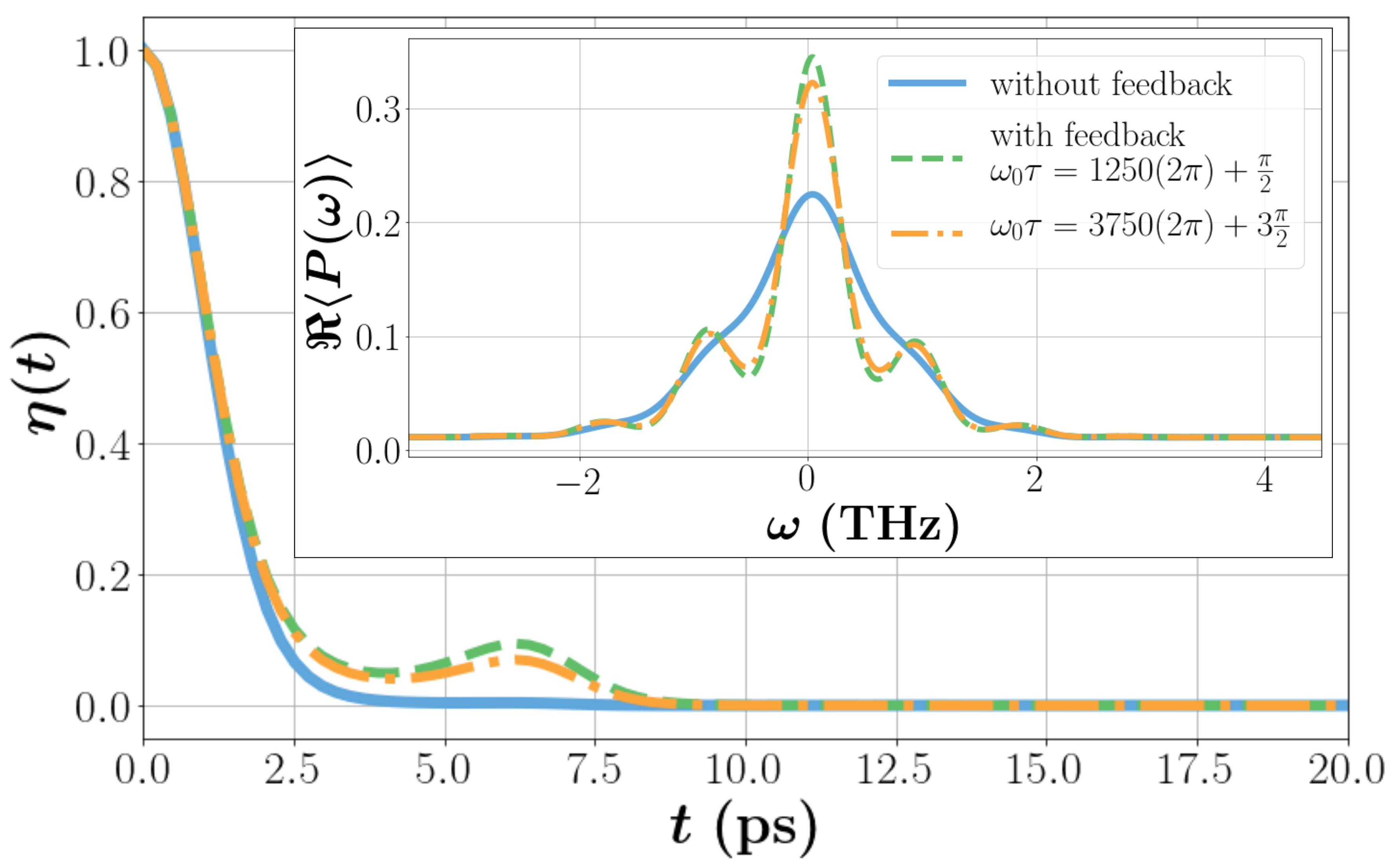
Figure 2: The normalized absolute value of the TLE coherence, $\eta(t)$, as a function of time, with and without feedback, at 300 K. Inset: The corresponding absorption spectra. Parameters: $\omega_{0}=1$ THz, $D=200$ GHz, $\kappa=20$ GHz, $\kappa\tau=157.1\times\{1,3\}$ (with feedback).

III Example (i): LB exposed to Markovian loss

Let us consider the reservoir coupling in the Markovian limit, $g_{k}=g_{0}$, and assume the same initial temperature for the reservoir and the cavity. In order to include temperature, we use the canonical statistical operator $\rho_{R}(0,T)=\exp[\sum_{k}\hbar\omega_{k}\hat{r}^{\dagger}_{k}(0)\hat{r}_{k}(0)/(k_{B}T)]/Z$, giving the following contributions,

$$\sigma_{R}(t) =\exp{\left\{-\frac{1}{2}\int|N_{k}(t)|^{2}\left[2n_{k}(T)+1\right]dk\right\}},$$

$$\sigma_{b}(t) =\exp{\left\{-\frac{1}{2}|\gamma(t)|^{2}\left[2n_{b}(T)+1\right]\right\}},$$

where $n_{k}(T)$ and $n_{b}(T)$ are the average occupation of the reservoir and LB modes at temperature $T$, respectively,

$$n_{b} =\frac{1}{e^{\frac{\hbar\omega_{0}}{kT}}-1} n_{k} =\frac{1}{e^{\frac{\hbar\omega_{k}}{kT}}-1}$$

The blue, solid curves in Fig. 2 show the corresponding time trace $\eta(t)$ and its Fourier transform (inset). The latter is proportional to the absorption spectrum $\mathcal{R}[\boldsymbol{\big{\langle}}\hat{P}(\omega)\boldsymbol{\big{\rangle}}]$, and is shown for parameters of a high-$\mathcal{Q}$ phonon cavity, in the regime of realizable experimental platforms on nanofabricated hybrid-systems De Alba et al. (2016); Rozas et al. (2009); Fainstein et al. (2013).

Due to the Markovian reservoir, the coherence decays monotonically in proportion to the coupling strength $g_{0}^{2}$. The coherence is irreversibly lost to the reservoir modes for longer times ($\kappa t\gg 1$) and, for the case shown in Fig. 2, LB side-peaks or “satellites” in the absorption spectrum are broadened and barely noticeable due to the dissipation produced by the structureless reservoir, as expected Chernyak and Mukamel (1996); Knox et al. (2002).

III.1 Recovering the independent boson model

A special case of the Markovian reservoir calculations is when we consider the temperature limit of $T=0$ for the reservoir, while keeping a finite temperature for the link boson. In this case, one finds

$$\text{Tr}\left\{\hat{\rho}^{d}_{P}(t)\right\}=\frac{1}{2}\exp\left\{-\,\Theta(t)\frac{|D|^{2}}{|B|^{2}}\left[2B^{*}t+n_{b}\left(1+e^{-2\kappa t}\right)+\frac{1}{2}\left(3-e^{-2\kappa t}\right)+i\frac{\omega_{0}^{2}}{|B|^{2}}\sin(\omega_{0}t)e^{-\kappa t}-\right.\right.$$ (28)

$$\hskip 147.95424pt\left.\left.-\left(2n_{b}+1\right)\cos(\omega_{0}t)e^{-\kappa t}+\frac{2\kappa}{|B|^{2}}\left(-2B^{*}+B^{*}e^{-Bt}+Be^{-B^{*}t}\right)\right]+\right.$$

$$\hskip 91.04872pt\left.+i\,\Theta(t)\frac{|D|^{2}}{|B|^{2}}\left[\left\{3\kappa\sin(\omega_{0}t)+4\omega_{0}\cos(\omega_{0}t)\right\}\frac{\kappa}{|B|^{2}}e^{-\kappa t}-\frac{\omega_{0}}{2\kappa}\left(1-e^{-2\kappa t}\right)\right]\right\}.$$ (29)

The last row of this formula (29) shows a shift of the satellites in the absorption spectrum compared to the expected values. These can become substantial if the couplings between the link boson and the emitter ($D$) or the reservoir ($g_{0}$) are comparable to the link boson frequency ($\omega_{0}$).

Without particle exchange with the environment, considering only pure dephasing, further simplification is possible. In this case the LB is not interacting with the reservoir at all $(g_{0},\kappa\rightarrow 0)$ and thus we arrive at the formula

$$\hat{\rho}_{P}^{\text{ibm}}(t)= \ \sigma_{e}(0)\exp\left\{i\frac{D^{2}}{\omega_{0}}t-\frac{D^{2}}{\omega_{0}^{2}}\left[(1+n_{b})(1-e^{-i\omega_{0}t})+n_{b}\left(1-e^{i\omega_{0}t}\right)\right]\right\},$$ (30)

which is the result known from the independent boson model Nazir and McCutcheon (2016); Krummheuer et al. (2002).

IV Example (ii): LB exposed to non-Markovian quantum feedback

The dynamics changes significantly when the link boson couples to a structured reservoir. The strength of the approach developed in this work is that we can treat such a reservoir with finite occupation and with an assumed boundary condition (here at $L$ Krummheuer et al. (2005)). The distant, perfectly reflecting mirror depicted in Fig. 1(c) introduces coherent feedback into the S-LB dynamics, as well as an entangled reservoir-LB dynamics Faulstich et al. (2018).

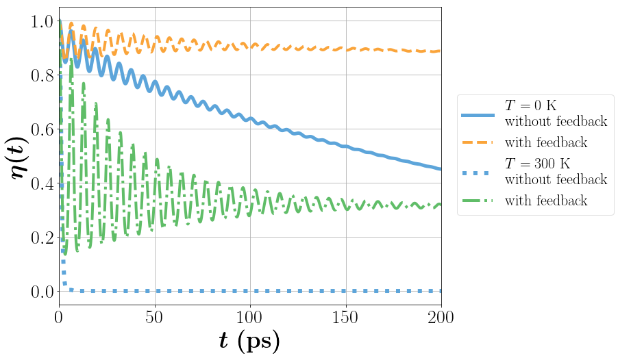
Figure 3: Time-evolution of the normalized coherence, $\eta(t)$, with and without feedback, and for different temperatures. Parameters: $\omega_{0}=1$ THz, $D=200$ GHz, $\kappa=20$ GHz, $\kappa\tau=0.031$.

This coherent feedback Zhang et al. (2017), originally introduced as an all-optical feedback Wiseman and Milburn (1994) for quantum systems, has been proven an efficient way to recover lost quantum information from a reservoir with infinite degrees of freedom. Besides introducing a distant mirror, as just described Faulstich et al. (2018), it can also be considered as a special case of cascaded quantum systems, as illustrated in Fig. 1(d) and described in Whalen et al. (2017)

For optical excitations, the effect of feedback first manifests itself as a reduction in the effective cavity linewidth. In certain regimes, the time-delay associated with the feedback propagation also becomes an important dynamical control parameter. This was used to enhance intrinsic quantum properties of various systems, such as squeezing Gough and Wildfeuer (2009); Iida et al. (2012); Kraft et al. (2016); Német and Parkins (2016), or to recover Rabi oscillations Kabuss et al. (2015). It has also proven to be useful for the manipulation of steady state behaviour of a given quantum system Német and Parkins (2016); Grimsmo et al. (2014) and to prepare various quantum states Kashiwamura and Yamamoto (2018). Here, for the LB-feedback case, we examine two limiting cases: the long-delay (Fig. 2) and short-delay (Fig. 3) limits.

In the long-delay limit ($\kappa\tau\gg 1$), the feedback loop reduces the decay rate of the coherence. In Fig. 2 (dashed and dashed-dotted lines) the LB-TLE interference is restored in the time-domain due to the feedback mechanism. This appears as a reduced effective linewidth of the LB-satellites in the absorption spectrum. However, we see that the feedback phase, i.e., the specific position of the reflecting surface $(\omega_{0}\tau=2k_{0}L)$ has only a weak impact; in particular, the green (dashed) and orange (dashed-dotted) lines in Fig. 2 are almost identical. The only difference arises from the fact that for decreasing delay, it is more probable that the TLE and the LB interact, as the cavity is more likely to be excited at a given point in time. However, generally, in the long-delay limit $(\kappa\tau\gg 1)$, the LB excitation is absorbed entirely by the reservoir before being fed back. Thus, the significance of the specific phase $\omega_{0}\tau$ is negligible and, in fact, eventually the whole coherence is lost into the reservoir regardless of the reduced, effective linewidth.

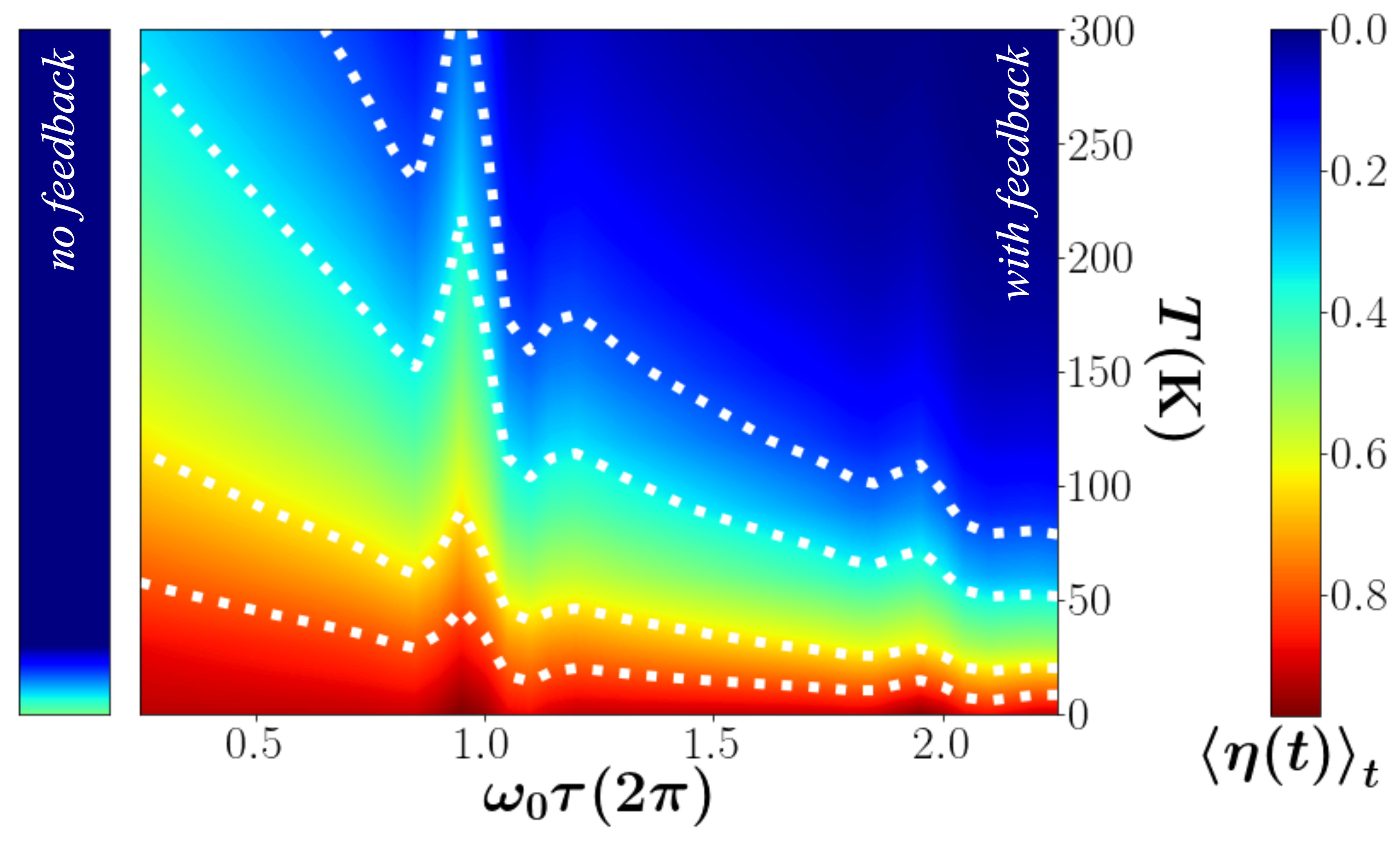
Figure 4: Colormap of the normalized coherence, $\eta(t)$, at $t=200$ ps. Without feedback the system decoheres rapidly at higher temperatures, whereas with feedback a finite coherence is preserved even at room temperature. Parameters: $\omega_{0}=1$ THz, $D=200$ GHz, $\kappa=20$ GHz.

On the other hand, in the case of short delay ($\kappa\tau\ll 1$), quantum interferences occur between the LB and the reservoir. This is because, with decreasing time delay $\tau$, there is a higher chance that the feedback signal observes a finite LB-excitation. This results in an oscillating coherence of the TLE, which shows the recovered coherent dynamics of the LB and the system; see Fig. 3 (dashed and dash-dotted lines). The introduced memory of the environment preserves a large portion of the initial coherence of the TLE, in contrast to the case without feedback, when all coherence is inevitably lost. This effect arises even for an initial thermal state of the LB and reservoir; see Fig. 3. Note that, however, the amount of leftover coherence decreases with growing temperature of the phonon reservoir, as shown in Fig. 4 (see also Nazir and McCutcheon (2016)), although, interestingly, persistence of the initial coherence can hold up to very high temperatures, in contrast to the case without feedback, where the coherence is damped even at $T=0$ due to spontaneous emission of the LB into its reservoir.

IV.1 Influence of the feedback phase

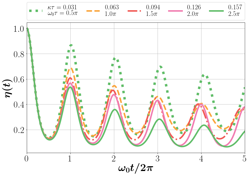
Figure 5: Time-evolution of the coherence with feedback for different time-delays. Parameters: $T=300$ K, $\omega_{0}=1$ THz, $D=200$ GHz, $\kappa=20$ GHz.

In the case of time-delayed coherent feedback, a short feedback length means that the accumulated propagation phase ($\omega_{0}\tau$) becomes an important control parameter. At phases described by $n\pi$, where $n\in\{1,2,...\}$ we recover oscillations with the LB frequency ($\omega_{0}$), whereas the frequency slightly changes for other phases, as can be observed in Fig. 5 for feedback phases $(n-1/2)\pi$.

Note that the feedback phase has a less significant effect on the amount of leftover coherence than the length of the corresponding time-delay. Its contribution becomes visible mainly in the frequency of oscillations and in the amplitude of recovered oscillations. The greater these oscillations are, the larger is the deviation from the mean value in the normalized coherence over the time period shown in Fig. 3. Thus we calculated the standard deviation of $\eta(t)$ as in eq.(18) over the first 200 ps as a function of temperature and propagation phase (Fig. 6).

Note that for lower temperatures, even though the steady state coherence is substantial (Fig. 3), the amplitude of the oscillations is quite small. This also shows up in Fig. 6, where signs of significant oscillations can only be seen for temperatures above $50$ K. The "hot spots" coincide well with the propagation phases, where a peak can be observed in the recovered coherence in Fig. 4, i.e., at multiples of $2\pi$.

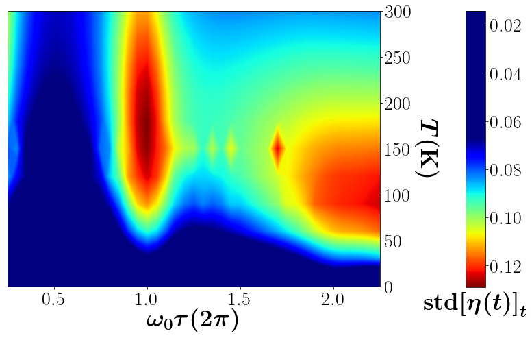
Figure 6: The deviation of the normalized coherence, $\eta(t)$, from its mean value over the time period of 200 ps as a function of temperature and feedback phase. In the case of constructive interference (integer multiples of $2\pi$), more pronounced oscillations can be observed, which appear as "hot spots" in the figure. On the other hand, for destructive interference (odd integer multiples of $\pi$), the amplitudes of the recovered oscillations are smaller, which appear as a smaller deviation from the mean value. Parameters: $T=300$ K, $\omega_{0}=1$ THz, $D=200$ GHz, $\kappa=20$ GHz.

V Conclusion

We have given a general framework for the description of structured-reservoir-induced quantum dynamics via the introduction of an additional link boson interaction, $\hat{H}_{LB}$, to the system Hamiltonian $\hat{H}_{S}$. In the case of a TLE coupled to the LB, an analytical expression is obtained for the resulting unconventional dephasing dynamics. Due to the analytical nature of the solutions, this method is readily capable of treating arbitrary initial states for both the LB and the reservoir. For example, one may consider initial Fock-state excitation of the LB ( see Appendix C).

Our investigations demonstrate a robust recovery of LB-system oscillations in a continuous environment with structured coupling. In the short-delay limit the propagation phase in the feedback loop $(\omega_{0}\tau)$ becomes an important control parameter, influencing both the frequency and amplitude of the recovered oscillations.

We also show that using this specific interaction between the LB and the environment, the initial coherence of the electronic system can be stabilized even at finite temperatures. Thus the introduced theoretical description opens up a new horizon for reservoir manipulation as, to the best of our knowledge, calculations for a quantum system with time-delayed coherent feedback at a finite temperature have not been performed before.

Appendix A Derivation of the coefficients in the linear map with feedback

The main point of taking the interaction picture is to describe the environment’s influence on the system only through its coupling to the LB by introducing an effective time dependence. The interaction picture Hamiltonian is considered as

$$\hat{H}_{I}/\hbar=\hat{H}_{R}/\hbar+\hat{H}_{S}/\hbar=$$ (31)

$$\hskip 11.38092pt=\hat{H}_{S}/\hbar+\omega_{0}\hat{b}^{\dagger}\hat{b}\ +\int\left[\omega_{k}\hat{r}^{\dagger}_{k}\hat{r}_{k}+g_{k}(\hat{r}^{\dagger}_{k}\hat{b}+\hat{b}^{\dagger}\hat{r}_{k})\right]dk,$$

from which the following equations of motion can be derived for the reservoir operators and the LB:

$$\dot{\hat{b}} =-i\omega_{0}\hat{b}(t)-i\int g_{k}\hat{r}_{k}(t)dk,$$

$$\dot{\hat{r}}_{k} =-i\omega_{k}\hat{r}_{k}(t)-ig_{k}\hat{b}(t).$$

Note that, by changing $g_{k}$ to $g_{0}$, we obtain the usual Markovian time-evolution. By formally integrating the second equation and substituting it back into the equation of motion for the LB, we obtain the following:

$$\dot{\hat{b}}= -i\omega_{0}\hat{b}(t)-i\int g_{k}e^{-i\omega_{k}t}\hat{r}_{k}(t)dk-$$

$$-\int_{0}^{t}\hat{b}(t^{\prime})\int g_{k}^{2}e^{-i\omega_{k}(t-t^{\prime})}dkdt^{\prime}.$$

The last term describes the environmental back-action on the state of the link-boson. Introducing a specific boundary condition for the problem results in a coherent feedback $\left(g_{k}=g_{0}\sin{(kL)}=g_{0}\sin{\left(\frac{\omega_{k}\tau}{2}\right)}\right)$ and a spectral density Petruccione et al. (2007)

$$J(\omega_{k})=\sin^{2}{\left(\frac{\omega_{k}\tau}{2}\right)}e^{-i\omega_{k}(t-t^{\prime})}=$$ (32)

$$\hskip 5.69046pt=\frac{1}{2}\left(e^{-i\omega_{k}(t-t^{\prime})}+\frac{1}{2}e^{-i\omega_{k}(t-t^{\prime}+\tau)}+\frac{1}{2}e^{-i\omega_{k}(t-t^{\prime}-\tau)}\right),$$

where the first term describes the standard Markovian decay, the second refers to a non-causal dependence, and the last term describes the past state of the link boson field fed back by the environment. Integrating over the frequencies and taking causality into account, we obtain the following for the environmental back action,

$$-\int_{0}^{t}\hat{b}(t^{\prime})\int g_{0}^{2}J(\omega_{k})dkdt^{\prime} =\frac{g_{0}^{2}\pi}{2c}\int_{0}^{t}\hat{b}(t^{\prime})\left[\delta(t-{t^{\prime}}+\tau)+\delta(t-{t^{\prime}}-\tau)-2\delta(t-{t^{\prime}})\right]dt=\kappa\left[\hat{b}(t-\tau)-\hat{b}(t)\right].$$

Thus, the equation of motion for the LB with the effective action of the environment becomes

$$\dot{\hat{b}}= -B\hat{b}(t)-i\int g_{k}e^{A_{k}t}\hat{r}_{k}(0)dk+$$

$$+\kappa\Theta(t-\tau)\hat{b}(t-\tau),$$ (33)

where we use

$$B =i\omega_{0}+\kappa,\hskip 28.45274ptA_{k}=-i\omega_{k},\hskip 28.45274pt\kappa=\frac{\pi g_{0}^{2}}{2c}.$$

The usual way of dealing with time-delayed dynamic equations is to apply the method of steps, where the solution is evaluated for each $\tau$-interval by first ignoring the delay-term and then substituting the solution obtained for the previous $\tau$-interval into the last term.

Let us follow this through the example of the first two $\tau$-intervals. For $0<t<\tau$ we have the following equation of motion,

$$\dot{\hat{b}} =-B\hat{b}(t)+\int D_{k}(t)\hat{r}_{k}(0)dk,$$

$$D_{k}(t) =-ig_{k}e^{A_{k}t},$$

for which we can obtain the solution

$$\hat{b}(t) =e^{-Bt}\hat{b}(0)+\int G_{0}^{k}(t)\hat{r}_{k}(0)dk,$$

$$G_{0}^{k}(t) =\int_{0}^{t}D_{k}(t^{\prime})e^{-B(t-t^{\prime})}d{t^{\prime}}=-\frac{ig_{k}}{A_{k}+B}\left(e^{A_{k}t}-e^{-Bt}\right).$$

By exchanging $g_{k}$ for the $k$-independent $g_{0}$, this recovers the Markovian coefficient $G^{d}_{k}(t)$ as in Eq. (5) in the main text. Substituting the above solution back into the last term of Eq. (A) gives the following equation of motion for the time-interval $0<t<2\tau$,

$$\dot{\hat{b}}= -B\hat{b}(t)+\kappa\Theta(t-\tau)\hat{b}(t-\tau)+$$

$$+\int\left[D_{k}(t)\kappa\Theta(t-\tau)G_{0}^{k}(t-\tau)\right]\hat{r}_{k}(0)dk,$$

for which we can obtain the solution

$$\hat{b}(t) =\left[\Theta(t)e^{-Bt}+\kappa\Theta(t-\tau)e^{-B(t-\tau)}(t-\tau)\right]\hat{b}(0)+$$

$$\hskip 14.22636pt+\int\left[\Theta(t)G_{0}^{k}(t)+\Theta(t-\tau)G_{1}^{k}(t)\right]\hat{r}_{k}(0)dk,$$

$$G_{1}^{k}(t) =\kappa\int^{t}_{\tau}G_{0}^{k}({t^{\prime}}-\tau)e^{-B(t-{t^{\prime}})}d{t^{\prime}}=$$

$$=-\frac{ig_{k}\kappa}{(A_{k}+B)^{2}}\left\{e^{A_{k}(t-\tau)}-\right.$$

$$\left.\hskip 71.13188pt-e^{-B(t-\tau)}\left[1+(A_{k}+B)(t-\tau)\right]\right\}.$$

Continuing in a similar fashion with the other time-intervals, the following ansatz can be assumed for a general coefficient $G_{m}^{k}(t)$:

$$G_{m}^{k}(t)= -\frac{ig_{k}\kappa^{m}}{(A_{k}+B)^{m+1}}\left[e^{A(t-m\tau)}-\right.$$

$$\left.\hskip 28.45274pt-e^{-B(t-m\tau)}\sum_{n=0}^{m}\frac{(t-m\tau)^{n}}{n!}(A_{k}+B)^{n}\right].$$

The next step in our derivation is to prove that by using the general recursive method demonstrated for $G_{1}^{k}(t)$, we obtain the next coefficient in the same form ($M=m+1$):

$$G_{M}^{k}(t) =\kappa\int_{(m+1)\tau}^{t}G_{m}^{k}({t^{\prime}}-\tau)e^{-B(t-{t^{\prime}})}d{t^{\prime}}=$$

$$=-\frac{ig_{k}\kappa^{M}e^{-Bt}}{(A_{k}+B)^{M}}\left[\int_{M\tau}^{t}e^{(A_{k}+B)\left({t^{\prime}}-M\tau\right)}e^{BM\tau}dt^{\prime}-e^{BM\tau}\sum_{n=0}^{m}\frac{(A_{k}+B)^{n}}{n!}\int_{M\tau}^{t}\left({t^{\prime}}-M\tau\right)^{n}d{t^{\prime}}\right]=$$

$$=-\frac{ig_{k}\kappa^{M}e^{-B(t-M\tau)}}{(A_{k}+B)^{M}}\left[\frac{e^{(A_{k}+B)(t-M\tau)}-1}{A_{k}+B}-\sum_{n=0}^{m}\frac{(A_{k}+B)^{n}}{n!}\frac{(t-M\tau)^{n+1}}{n+1}\right]=$$

$$=-\frac{ig_{k}\kappa^{M}}{(A_{k}+B)^{M+1}}\left[e^{A(t-M\tau)}-e^{-B(t-M\tau)}\sum_{n=0}^{M}\frac{(t-M\tau)^{n}}{n!}(A_{k}+B)^{n}\right].$$

For the coefficients of $\hat{b}(0)$ a similar process leads to the general formula

$$F_{m}(t)=\frac{\kappa^{m}}{m!}e^{-B(t-m\tau)}(t-m\tau)^{m}.$$

By summing up these contributions as

$$F_{fb}(t)=\sum_{m=0}^{\infty}\Theta(t-m\tau)F_{m}(t),$$

$$G_{k}^{fb}(t)=\sum_{m=0}^{\infty}\Theta(t-m\tau)G_{m}^{k}(t),$$

we obtain the final form of the coefficients given in the main text in Eqs. (6,7).

Appendix B Alternative derivation for a pure dephasing interaction

Since time-dependence of $\hat{H}_{LB}(t)$ can be expressed solely by $c$-number functions and initial operators that are time-independent, (Eq. (4-7)), an exact formula can be obtained for the dynamics of the observable $\hat{P}(t)$:

$$i\hbar\frac{\text{d}\hat{\rho}_{I}}{\text{dt}}\hat{P}(t) =\left[\hat{H}_{LB},\hat{\rho}_{I}\right]\hat{P}(t),$$

$$\frac{\text{d}\hat{\rho}_{I}}{\text{dt}}\hat{P}(t) =-iD\left[\hat{b}(t)+\hat{b}^{\dagger}(t)\right]\hat{P}^{\dagger}(t)\hat{P}(t)\hat{\rho}_{I}\hat{P}(t).$$ (34)

By exploiting the intrinsic linear dynamics of the TLE coherence (19) we obtain

$$\frac{\text{d}\hat{\rho}_{P}}{\text{dt}} =-i\hat{\mathcal{B}}(t)\hat{P}^{\dagger}(0)\hat{P}(0)\hat{\rho}_{P},$$ (35)

$$\hat{\mathcal{B}}(t) =\hat{b}^{\dagger}(t)+\hat{b}(t),$$ (36)

where we abbreviate $\hat{\rho}^{I}(t)\hat{P}(t)=:\hat{\rho}^{I}_{P}(t)$, and $\text{Tr}[\hat{\rho}^{I}_{\hat{P}}(t)]=\boldsymbol{\big{\langle}}\hat{P}(t)\boldsymbol{\big{\rangle}}$. A stroboscopic solution of the equation of motion for short enough time steps gives

$$\hat{\rho}_{P}(t+\Delta t)=\left(1-i\hat{\mathcal{B}}(t)\hat{P}^{\dagger}(0)\hat{P}(0)\Delta t\right)\hat{\rho}_{P}(t)\approx$$

$$\approx e^{-i\hat{\mathcal{B}}(t)\hat{P}^{\dagger}(0)\hat{P}(0)\Delta t}\,e^{-i\hat{\mathcal{B}}(t-\Delta t)\hat{P}^{\dagger}(0)\hat{P}(0)\Delta t}\hat{\rho}_{P}(t-\Delta t).$$

By applying the Baker-Campbell-Hausdorff formula, this translates into

$$\hat{\rho}^{I}_{\hat{P}}(t)=\exp\left[-i\int_{0}^{t}\hat{H}_{LB}(t_{1})dt_{1}\right]\times$$ (37)

$$\hskip 17.07182pt\times\exp\left[-\frac{1}{2}\int_{0}^{t}\int_{0}^{t_{1}}[\hat{H}_{LB}(t_{1}),\hat{H}_{LB}(t_{2})]dt_{2}dt_{1}\right]\hat{\rho}^{I}_{\hat{P}}(0),$$

which is the same as was obtained in (21).

Appendix C Initial Fock excitation in the LB

Let us assume $n$ bosons for the LB in the beginning $\left(\sigma_{LB}(0)=\left|n\right\rangle\left\langle n\right|\right)$ and 0 K for the reservoir. Then, the link boson part of the expectation value (26) becomes

$$\sigma_{LB}(t) =\sum_{m}\left\langle m\right|e^{-i\left[\gamma(t)\hat{b}(0)+\gamma^{*}(t)\hat{b}^{\dagger}(0)\right]}\left|n\right\rangle\left\langle n\right|\left|m\right\rangle=$$

$$=\left\langle n\right|e^{-i\left[\gamma(t)\hat{b}(0)+\gamma^{*}(t)\hat{b}^{\dagger}(0)\right]}\left|n\right\rangle.$$ (38)

If $n$ is set to $0$, we have a series, which results in the typical exponential evolution,

$$\sigma_{LB}(t)= \ \exp\left[-\frac{|\gamma(t)|^{2}}{2}\right],$$ (39)

which is equivalent to the zero temperature case. Higher Fock-state contributions can be calculated by using the Baker-Campbell-Hausdorff formula, since

$$[-i\gamma^{*}(t)\hat{b}^{\dagger}(0),-i\gamma(t)\hat{b}(0)]=|\gamma(t)|^{2},$$ (40)

thus the link boson part of the expectation value becomes

$$\sigma_{LB}(t)= \left\langle n\right|e^{-i\gamma^{*}(t)\hat{b}^{\dagger}(0)}e^{-i\gamma(t)\hat{b}(0)}\left|n\right\rangle e^{-\frac{|\gamma(t)|^{2}}{2}},$$ (41)

which can be evaluated as

$$\sigma_{LB}(t) =\left(\left\langle n\right|e^{-i\gamma^{*}(t)\hat{b}^{\dagger}(0)}\right)\left(e^{-i\gamma(t)\hat{b}(0)}\left|n\right\rangle\right)e^{-\frac{|\gamma(t)|^{2}}{2}}=$$

$$=\left(\left\langle n\right|\sum_{l=0}^{n}\frac{\left[-i\gamma^{*}(t)\hat{b}^{\dagger}(0)\right]^{l}}{l!}\right)\left(\sum_{l^{\prime}=0}^{n}\frac{\left[-i\gamma(t)\hat{b}(0)\right]^{l^{\prime}}}{l^{\prime}!}\left|n\right\rangle\right)e^{-\frac{|\gamma(t)|^{2}}{2}}=$$

$$=\sum_{l=0}^{n}\frac{\left[-|\gamma(t)|^{2}\right]^{l}}{l!}\binom{n}{l}e^{-\frac{|\gamma(t)|^{2}}{2}}.$$

References

- Nielsen and Chuang (2010) M. A. Nielsen and I. L. Chuang, 10th Anniv. Ed. (Cambridge University Press, 2010).
- Gardiner and Zoller (2015) C. Gardiner and P. Zoller, The Quantum World of Ultra-Cold Atoms and Light Book II: The Physics of Quantum-Optical Devices (World Scientific, 2015) pp. 1–524.
- Zubairy and Scully (1997) M. S. Zubairy and M. O. Scully, Quantum Optics (Cambridge University Press, 1997).
- Zoller et al. (2005) P. Zoller, T. Beth, D. Binosi, et al., Eur. Phys. J. D 36, 203 (2005).
- Walls and Milburn (2008) D. Walls and G. Milburn, Quantum Optics, SpringerLink: Springer e-Books (Springer Berlin Heidelberg, 2008).
- May and Kühn (2008) V. May and O. Kühn, Charge and energy transfer dynamics in molecular systems (John Wiley & Sons, 2008).
- Bimberg (2008) D. Bimberg, ed., Semicond. Nanostructures (Springer-Verlag Berlin Heidelberg, 2008).
- Nazir and McCutcheon (2016) A. Nazir and D. P. S. McCutcheon, J. Phys. Condens. Matter 28, 103002 (2016), arXiv:1511.01405 .
- Iles-Smith et al. (2017) J. Iles-Smith, D. P. McCutcheon, A. Nazir, and J. Mørk, Nat. Photonics 11, 521 (2017), arXiv:1612.04173 .
- Förstner et al. (2003) J. Förstner, C. Weber, J. Danckwerts, and A. Knorr, Phys. Rev. Lett. 91, 127401 (2003).
- Förstner et al. (2003) J. Förstner, C. Weber, J. Danckwerts, and A. Knorr, Phys. Status Solidi B 238, 419 (2003).
- Roy-Choudhury and Hughes (2015) K. Roy-Choudhury and S. Hughes, Phys. Rev. B 92, 205406 (2015), arXiv:1504.03356v1 .
- Roy and Hughes (2011) C. Roy and S. Hughes, Phys. Rev. X 1, 021009 (2011).
- Harsij et al. (2012) Z. Harsij, M. Bagheri Harouni, R. Roknizadeh, and M. H. Naderi, Phys. Rev. A 86, 063803 (2012).
- Hughes and Carmichael (2013) S. Hughes and H. J. Carmichael, New J. Phys. 15, 053039 (2013), arXiv:1210.0488 .
- Weiler et al. (2012) S. Weiler, A. Ulhaq, S. M. Ulrich, D. Richter, M. Jetter, P. Michler, C. Roy, and S. Hughes, Phys. Rev. B 86, 241304(R) (2012), arXiv:1207.4972 .
- Wigger et al. (2014) D. Wigger, S. Lüker, D. E. Reiter, V. M. Axt, P. Machnikowski, and T. Kuhn, J. Phys. Condens. Matter 26, 355802 (2014), arXiv:1312.3754v2 .
- Carmele et al. (2013) A. Carmele, A. Knorr, and F. Milde, New J. Phys. 15, 105024 (2013), arXiv:1203.0126 .
- Wilson-Rae and Imamoğlu (2002) I. Wilson-Rae and A. Imamoğlu, Phys. Rev. B 65, 235311 (2002), arXiv:quant-ph/0105022 .
- Droenner et al. (2017) L. Droenner, N. L. Naumann, J. Kabuss, and A. Carmele, Phys. Rev. A 96, 043805 (2017), arXiv:1706.07777v2 .
- Martin et al. (2004) I. Martin, A. Shnirman, L. Tian, and P. Zoller, Phys. Rev. B 69, 125339 (2004), arXiv:cond-mat/0310229 .
- Jaehne et al. (2008) K. Jaehne, K. Hammerer, and M. Wallquist, New J. Phys. 10, 095019 (2008), arXiv:0804.0603v2 .
- Bounouar et al. (2015) S. Bounouar, M. Müller, A. M. Barth, M. Glässl, V. M. Axt, and P. Michler, Phys. Rev. B 91, 161302 (2015), arXiv:1408.7027 .
- Glässl et al. (2012) M. Glässl, L. Sörgel, A. Vagov, M. D. Croitoru, T. Kuhn, and V. M. Axt, Phys. Rev. B 86, 035319 (2012).
- Hameau et al. (1999) S. Hameau, Y. Guldner, O. Verzelen, R. Ferreira, G. Bastard, J. Zeman, A. Lemaitre, and J. M. Gérard, Phys. Rev. Lett. 83, 4152 (1999).
- Krauss and Wise (1997) T. D. Krauss and F. W. Wise, Phys. Rev. Lett. 79, 5102 (1997).
- Carmele et al. (2010) A. Carmele, M. Richter, W. W. Chow, and A. Knorr, Phys. Rev. Lett. 104, 156801 (2010).
- Fainstein et al. (2013) A. Fainstein, N. D. Lanzillotti-Kimura, B. Jusserand, and B. Perrin, Phys. Rev. Lett. 110, 037403 (2013).
- Lanzillotti-Kimura et al. (2015) N. D. Lanzillotti-Kimura, A. Fainstein, and B. Jusserand, Ultrasonics 56, 80 (2015).
- Trigo et al. (2002) M. Trigo, A. Bruchhausen, A. Fainstein, B. Jusserand, and V. Thierry-Mieg, Phys. Rev. Lett. 89, 227402 (2002), arXiv:cond-mat/0206488 .
- Kabuss et al. (2012) J. Kabuss, A. Carmele, T. Brandes, and A. Knorr, Phys. Rev. Lett 109, 054301 (2012).
- Pascual Winter et al. (2005) M. F. Pascual Winter, A. Fainstein, M. Trigo, T. Eckhause, R. Merlin, A. Cho, and J. Chen, Phys. Rev. B 71, 085305 (2005).
- Soykal et al. (2011) Ö. O. Soykal, R. Ruskov, and C. Tahan, Phys. Rev. Lett. 107, 235502 (2011), arXiv:1106.1654v3 .
- Anguiano et al. (2017) S. Anguiano, A. E. Bruchhausen, B. Jusserand, I. Favero, F. R. Lamberti, L. Lanco, I. Sagnes, A. Lemaître, N. D. Lanzillotti-Kimura, P. Senellart, and A. Fainstein, Phys. Rev. Lett. 118, 263901 (2017).
- Pirkkalainen et al. (2013) J.-M. Pirkkalainen, S. U. Cho, J. Li, G. S. Paraoanu, P. J. Hakonen, and M. A. Sillanpää, Nature 494, 211 (2013), arXiv:1207.1637 .
- Faulstich et al. (2018) F. M. Faulstich, M. Kraft, and A. Carmele, J. Mod. Opt. 65, 1323 (2018), arXiv:1703.05928 .
- Cassabois and Ferreira (2008) G. Cassabois and R. Ferreira, Comptes Rendus Phys. 9, 830 (2008).
- Moody et al. (2012) G. Moody, M. E. Siemens, A. D. Bristow, X. Dai, D. Karaiskaj, A. S. Bracker, D. Gammon, and S. T. Cundiff, Proc.SPIE 8260, 8260 (2012).
- Thoma et al. (2016) A. Thoma, P. Schnauber, M. Gschrey, M. Seifried, J. Wolters, J. H. Schulze, A. Strittmatter, S. Rodt, A. Carmele, A. Knorr, T. Heindel, and S. Reitzenstein, Phys. Rev. Lett. 116, 033601 (2016), arXiv:1507.05900 .
- Liu et al. (2018) J. Liu, K. Konthasinghe, M. Davanço, J. Lawall, V. Anant, V. Verma, R. Mirin, S. W. Nam, J. D. Song, B. Ma, Z. S. Chen, H. Q. Ni, Z. C. Niu, and K. Srinivasan, Phys. Rev. Appl. 9, 064019 (2018).
- Leggett et al. (1987) A. J. Leggett, S. Chakravarty, A. T. Dorsey, M. P. A. Fisher, A. Garg, and W. Zwerger, Rev. Mod. Phys. 59 (1987), 10.1103/RevModPhys.59.1.
- Besombes et al. (2001) L. Besombes, K. Kheng, L. Marsal, and H. Mariette, Phys. Rev. B 63, 155307 (2001).
- Favero et al. (2003) I. Favero, G. Cassabois, R. Ferreira, D. Darson, C. Voisin, J. Tignon, C. Delalande, G. Bastard, P. Roussignol, and J. M. Gérard, Phys. Rev. B 68, 233301 (2003).
- Petruccione et al. (2007) F. Petruccione, H. H.-P. Breuer, and F. Petruccione, The Theory of Open Quantum Systems (Oxford University Press, 2007).
- Krummheuer et al. (2002) B. Krummheuer, V. M. Axt, and T. Kuhn, Phys. Rev. B 65, 195313 (2002).
- Pazy (2002) E. Pazy, Semicond. Sci. Technol 17, 1172 (2002), arXiv:cond-mat/0212509v1 .
- Agarwal (2012) G. S. Agarwal, Quantum optics (Cambridge University Press, 2012).
- Ramos et al. (2013) T. Ramos, V. Sudhir, K. Stannigel, P. Zoller, and T. J. Kippenberg, Phys. Rev. Lett. 110, 193602 (2013), arXiv:1302.1855 .
- Law and Eberly (1996) C. K. Law and J. H. Eberly, Phys. Rev. Lett. 76, 1055 (1996).
- Rabl et al. (2009) P. Rabl, P. Cappellaro, M. V. Dutt, L. Jiang, J. R. Maze, and M. D. Lukin, Phys. Rev. B 79, 041302(R) (2009), arXiv:0806.3606 .
- Arcizet et al. (2011) O. Arcizet, V. Jacques, A. Siria, P. Poncharal, P. Vincent, and S. Seidelin, Nat. Phys. 7, 879 (2011), arXiv:1112.1291 .
- Armour et al. (2002) A. D. Armour, M. P. Blencowe, and K. C. Schwab, Phys. Rev. Lett. 88, 148301 (2002), arXiv:cond-mat/0112403 .
- Irish and Schwab (2003) E. K. Irish and K. Schwab, Phys. Rev. B 68, 155311 (2003), arXiv:cond-mat/0301252v2 .
- LaHaye et al. (2009) M. D. LaHaye, J. Suh, P. M. Echternach, K. C. Schwab, and M. L. Roukes, Nature 459, 960 (2009).
- Stadler et al. (2017) P. Stadler, W. Belzig, and G. Rastelli, Phys. Rev. B 96, 045429 (2017), arXiv:1703.05274 .
- Xue et al. (2007) F. Xue, Y. D. Wang, C. P. Sun, H. Okamoto, H. Yamaguchi, and K. Semba, New J. Phys. 9, 35 (2007), arXiv:cond-mat/0607180 .
- Etaki et al. (2008) S. Etaki, M. Poot, I. Mahboob, K. Onomitsu, H. Yamaguchi, and H. S. J. van der Zant, Nat. Phys. 4, 785 (2008).
- Khosla et al. (2018) K. E. Khosla, M. R. Vanner, N. Ares, and E. A. Laird, Phys. Rev. X 8, 021052 (2018), arXiv:1710.01920 .
- Johnson et al. (2010) B. R. Johnson, M. D. Reed, A. A. Houck, D. I. Schuster, L. S. Bishop, E. Ginossar, J. M. Gambetta, L. DiCarlo, L. Frunzio, S. M. Girvin, and R. J. Schoelkopf, Nat. Phys. 6, 663 (2010), arXiv:1003.2734 .
- Reiserer et al. (2013) A. Reiserer, S. Ritter, and G. Rempe, Science 342, 1349 (2013), arXiv:1311.3625 .
- Lemmer et al. (2018) A. Lemmer, C. Cormick, D. Tamascelli, T. Schaetz, S. F. Huelga, and M. B. Plenio, New Journal of Physics 20, 073002 (2018), arXiv:1704.00629 .
- Wilson-Rae et al. (2004) I. Wilson-Rae, P. Zoller, and A. Imamoğlu, Phys. Rev. Lett. 92, 075507 (2004), arXiv:cond-mat/0306724 .
- Yeo et al. (2013) I. Yeo, P.-L. de Assis, A. Gloppe, E. Dupont-Ferrier, P. Verlot, N. S. Malik, E. Dupuy, J. Claudon, J.-M. Gérard, A. Auffèves, G. Nogues, S. Seidelin, J.-P. Poizat, O. Arcizet, and M. Richard, Nat. Nanotechnol. 9, 106 (2013), arXiv:1306.4209 .
- Munsch et al. (2017) M. Munsch, A. V. Kuhlmann, D. Cadeddu, J.-M. Gérard, J. Claudon, M. Poggio, and R. J. Warburton, Nat. Commun. 8, 76 (2017), arXiv:1608.03082 .
- Pichler and Zoller (2016) H. Pichler and P. Zoller, Phys. Rev. Lett. 116, 093601 (2016), arXiv:1510.04646 .
- Whalen and Carmichael (2016) S. J. Whalen and H. J. Carmichael, Phys. Rev. A 93, 063820 (2016), arXiv:1602.03971 .
- Weiss (2012) U. Weiss, Quantum dissipative systems, Vol. 13 (World scientific, 2012).
- Huelga et al. (2012) S. F. Huelga, Á. Rivas, and M. B. Plenio, Phys. Rev. Lett. 108, 160402 (2012), arXiv:1106.2841 .
- Breuer and Petruccione (2002) H.-P. Breuer and F. Petruccione, The theory of open quantum systems (Oxford University Press on Demand, 2002).
- Kabuss et al. (2015) J. Kabuss, D. O. Krimer, S. Rotter, K. Stannigel, A. Knorr, and A. Carmele, Phys. Rev. A 92, 053801 (2015), arXiv:1503.05722 .
- Dorner and Zoller (2002) U. Dorner and P. Zoller, Phys. Rev. A 66, 023816 (2002), arXiv:quant-ph/0203147 .
- Kabuss et al. (2016) J. Kabuss, F. Katsch, A. Knorr, and A. Carmele, JOSA B 33, C10 (2016), arXiv:1512.05884 .
- Guimond et al. (2017) P.-O. Guimond, M. Pletyukhov, H. Pichler, and P. Zoller, Quantum Sci. Technol. 2, 044012 (2017), arXiv:1706.07844 .
- Feynman and Vernon Jr (2000) R. P. Feynman and F. Vernon Jr, Annals of physics 281, 547 (2000).
- Calarco et al. (2003) T. Calarco, A. Datta, P. Fedichev, E. Pazy, and P. Zoller, Phys. Rev. A 68, 012310 (2003).
- Borri et al. (2005) P. Borri, W. Langbein, U. Woggon, V. Stavarache, D. Reuter, and A. D. Wieck, Phys. Rev. B 71, 115328 (2005).
- Krügel et al. (2005) A. Krügel, V. Axt, T. Kuhn, P. Machnikowski, and A. Vagov, Appl. Phys. B 81, 897 (2005).
- Kaer et al. (2013) P. Kaer, P. Lodahl, A.-P. Jauho, and J. Mørk, Phys. Rev. B 87, 081308 (2013), arXiv:1203.6268 .
- Unsleber et al. (2015) S. Unsleber, D. P. S. McCutcheon, M. Dambach, M. Lermer, N. Gregersen, S. Höfling, J. Mørk, C. Schneider, and M. Kamp, Phys. Rev. B 91, 075413 (2015), arXiv:1503.00931 .
- Grimsmo et al. (2014) A. L. Grimsmo, A. S. Parkins, and B. S. Skagerstam, New J. Phys. 16, 065004 (2014), arXiv:1401.2287 .
- De Alba et al. (2016) R. De Alba, F. Massel, I. R. Storch, T. Abhilash, A. Hui, P. L. McEuen, H. G. Craighead, and J. M. Parpia, Nat. Nanotechnol. 11, 741 (2016), arXiv:1604.04605 .
- Rozas et al. (2009) G. Rozas, M. F. Pascual Winter, B. Jusserand, A. Fainstein, B. Perrin, E. Semenova, and A. Lemaitre, Phys. Rev. Lett. 102, 015502 (2009).
- Chernyak and Mukamel (1996) V. Chernyak and S. Mukamel, J. Chem. Phys. 105, 4565 (1996).
- Knox et al. (2002) R. S. Knox, G. J. Small, and S. Mukamel, Chem. Phys. 281, 1 (2002).
- Krummheuer et al. (2005) B. Krummheuer, V. M. Axt, and T. Kuhn, Phys. Rev. B 72, 245336 (2005).
- Zhang et al. (2017) J. Zhang, Y.-x. xi Liu, R.-B. B. Wu, K. Jacobs, and F. Nori, Phys. Rep. 679, 1 (2017), arXiv:1407.8536 .
- Wiseman and Milburn (1994) H. M. Wiseman and G. J. Milburn, Phys. Rev. A 49, 4110 (1994), arXiv:0409050 [quant-ph] .
- Whalen et al. (2017) S. J. Whalen, A. L. Grimsmo, and H. J. Carmichael, Quantum Sci. Technol 2, 044008 (2017), arXiv:1702.05776 .
- Gough and Wildfeuer (2009) J. E. Gough and S. Wildfeuer, Phys. Rev. A 80, 042107 (2009).
- Iida et al. (2012) S. Iida, M. Yukawa, H. Yonezawa, N. Yamamoto, and A. Furusawa, IEEE Transactions on Automatic Control 57, 2045 (2012).
- Kraft et al. (2016) M. Kraft, S. M. Hein, J. Lehnert, E. Schöll, S. Hughes, and A. Knorr, Phys. Rev. A 94, 023806 (2016), arXiv:1603.07137v1 .
- Német and Parkins (2016) N. Német and S. Parkins, Phys. Rev. A 94, 023809 (2016), arXiv:1606.00178 .
- Kashiwamura and Yamamoto (2018) Y. Kashiwamura and N. Yamamoto, Phys. Rev. A 97, 062341 (2018).