Nonovershooting Cooperative Output Regulation for Linear Multi-Agent Systems

Abstract

We consider the problem of cooperative output regulation for linear multi-agent systems. A distributed dynamic output feedback design method is presented that solves the cooperative output regulation problem and also ensures that all agents track the desired reference signal without overshoot in their transient response.

I Introduction

In this paper, we consider a family of $N$ linear multi-variable systems ruled by the equations

$$\Sigma_{i}:\begin{cases}\dot{x}_{i}(t)=A_{i}x_{i}(t)+B_{i}u_{i}(t)+E_{i}w(t),\;\;\;x_{i}(0)=x_{i,0}\\ y_{i}(t)=C_{y,_{i}}x_{i}(t)+{D_{y,i}u_{i}(t)},+H_{y,i}w(t)\\ e_{i}(t)=C_{e,i}x_{i}(t)+D_{e,i}u_{i}(t)+H_{e,i}w(t)\par\end{cases}$$ (1)

where, for all $t\geq 0$, the signal $x_{i}(t)\in^{n_{i}}$ is the state, $u_{i}(t)\in^{m_{i}}$ is the control input, $y_{i}(t)\in^{p_{i}}$ is the measured output, and $e_{i}(t)\in^{\rho_{i}}$ is the regulated output of the $i$-th system, for $i\in\{1,\dots,N\}$. The exogenous signal $w(t)\in^{q}$ represents a reference signal to be tracked or a disturbance signal to be rejected, and is assumed to be generated by an exosystem

$$\dot{w}=Sw,\quad w(0)=w_{0}$$ (2)

All matrices appearing in (1) are appropriate dimensional constant matrices. We assume the $N$ agents are divided into two groups. The first informed group consists of systems $\Sigma_{i}$, for $i\in\{1,\dots,l\}$, that can access information about $w$ from the measured output $y_{i}$, which implies $H_{y,i}\neq 0$. The second uninformed group of systems $\Sigma_{i}$, for $i\in\{l+1,\dots,N\}$, for which $H_{y,i}=0$, cannot directly access information about $w$.

The problem of cooperative output regulation for multi-agent systems involves designing control inputs $u_{i}$ such that the overall system is asymptotically stable for the case $w=0$, and such that the tracking errors $e_{i}$ all converge to zero, ensuring the outputs of all the agents converge asymptotically to the desired reference signal. For the special case of a single system ($N=1$), with access to measurements of the exogenous signal, the problem reduces to the classic problem of output feedback regulation. This problem is central to modern control theory. Solvability conditions and extensive compilations of results are given in [1]. It is assumed that the measured output $y_{i}$ is available for controller design.

The problem of output regulation of multi-agent systems has been the subject of a number of papers recently [2]-[6]. As some of the agents cannot access the exogenous signal, the problem cannot be solved by the methods of the classical output regulation. In [5], Su and Huang considered the system (1) under the assumption that all states of each system can be measured and are available for use in the control input; this occurs when $p_{i}=n_{i}$. They proposed a distributed dynamic state feedback control scheme and gave conditions under which the multi-agent cooperative regulation problem could be solved. They showed that their problem framework and controller architecture could accommodate the methods of [2] and [3] as special cases. In [6], Su and Huang extended the state feedback methods of [5] to the case where $p_{i}<n_{i}$ using a distributed dynamic measurement feedback control architecture.

For many control systems there is a need to avoid undesirable transient phenomena such as high-frequency oscillations and large magnitudes of the output [7]. For a multi-agent example system, we may consider the lateral and directional control of a research aircraft known as MuPAL-$\alpha$. The flight dynamics of this aircraft were described in [8], and [9] considered the control of four such aircraft within a network. The control objective was for all the aircraft to simultaneously track a given sideways velocity and a given roll angle. Exceeding the desired sideways velocity in a platoon may cause some aircraft to fly too close together, and possibly collide. If an aircraft exceeds its desired roll angle, its flight may become unstable and possibly crash.

Thus a desirable transient response should seek to minimise, or else avoid entirely, overshoot in the tracking signal. The problem of overshoot is related to the problem of string stability for automated platoons of vehicles [10, 11]. Such platoons are usually assumed to be subject to disturbances which should be rejected. Moreover, one of the objectives for them is to track a reference velocity. Obviously, if any of the vehicles in the platoon overshoot in their velocity, collisions might occur. Numerous papers have appeared recently seeking to improve the transient performance in the tracking control of multi-agent systems, including the use of consensus protocols [12]-[13], composite nonlinear feedback control [14], travelling waves [15], iterative learning control [16] and transient synchronization [17]. We note however that none of these papers offered a method for entirely avoiding overshoot in all outputs for all the agents.

The design of control laws to achieve a nonovershooting step response for a single linear time invariant (LTI) plant was considered in the paper [18] by the first author of the present paper. Several methods were given for the design of a linear state feedback control law to deliver a nonovershooting step response for an LTI multiple-input multiple-output (MIMO) system. This requires the closed-loop system to be stable, and that the tracking error of the step response converges to zero without changing sign in any of its components. In [19], the methods were adapted to the problem of avoiding undershoot in the step response, and in [20] the methods were used to achieve nonovershooting output regulation. The design methods of [18] and [19] have been incorporated into a public domain MATLAB${}^{\textrm{\tiny{\textregistered}}}$ toolbox, known as NOUS [21].

In this paper, we consider how to combine the nonovershooting tracking control methods of [18] with the distributed control scheme of [6] to solve the multi-agent cooperative output regulation problem in such a manner that all agents achieve exact output regulation with a nonovershooting transient response. The principal contribution of the paper is to identify the necessary system assumptions and information required in order for the control scheme to deliver a nonovershooting response. The authors believe that this is the first paper offering a control scheme to avoid overshoot in all outputs of all agents of a multi-agent system.

The paper is organised as follows. In Section II, we introduce some elementary notions from graph theory that enable us to define our multi-agent problem. In Section III, we introduce the dynamic measurement output feedback control architecture introduced by [6], and define our nonovershooting cooperative output regulation problem. In Section III-B, we briefly discuss the nonovershooting controller design methods of [18]. The main result of the paper is presented in Section IV, where we show how the methods of [18] can be employed within the controller architecture of [6] to solve our problem.

Section V demonstrates the application of the control method to the lateral and directional control of a network of research aircraft known as MuPAL-$\alpha$, as discussed in [9]. Our simulations demonstrate that the methods introduced in this paper can effectively avoid overshoot in all the outputs of all the agents involved in the flight simulation. Finally Section VII offers some concluding thoughts.

Notation. $I_{n}$ is the $n$-dimensional identity matrix, and ${\bf 0}_{N\times l}$ denotes an $N\times l$ matrix with zero entries. For a square matrix $A$, we use $\rho(A)$ to denote its spectrum. We say that a square matrix $A$ is Hurwitz if $\rho(A)$ lies within the open left-hand complex plane. $Re(\lambda)$ denotes the real part of a complex scalar $\lambda$, and $\otimes$ denotes the Kronecker product of matrices.

II Mathematical Preliminaries

II-A Graph Theory

Graph theory [22] has been widely used to describe the topology of networked systems by means of vertices and edges. Let ${\cal G}({\cal V},{\cal E},a)$ denote a weighted digraph, in which ${\cal V}$ is the finite set of nodes, ${\cal E}$ is the set of directed edges, and $a$ represents the set of weights for each edge. Directed edges have a head node and a tail node. We use $(j,i)$ to denote the edge in ${\cal E}$ directed from tail node $j$ to head node $i$, and $a_{ij}$ denotes the weighting assigned to this edge. For node $i\in{\cal V}$, we use ${\cal N}_{i}$ to denote all nodes $j\in{\cal V}$ for which there exists an edge from tail node $j$ to head node $i$. Thus

$${\cal N}_{i}=\{j\in{\cal V}:(j,i)\in{\cal E}\}$$ (3)

We refer to the nodes in ${\cal N}_{i}$ as the neighbours of node $i$. A digraph has a spanning tree if there exists at least one node having a directed path to all the other nodes. The in-degree of a node, denoted by $d_{in}(i)$, is the sum of the weights of the edges with heads at that node, and is given by

$$d_{in}(i)=\sum_{j\in{\cal N}_{i}}\ a_{ij}$$ (4)

The degree matrix of a digraph is a diagonal matrix ${\cal D}$, whose diagonal entries are the in-degrees of the nodes of the digraph from which it is derived. The weighted adjacency matrix ${\cal A}$ for a digraph has entries ${\cal A}_{ij}$ given by

$${\cal A}_{ij}=\begin{cases}a_{ij},&(j,i)\in{\cal E}\\ 0,&\mbox{ otherwise}\end{cases}$$ (5)

The information contained within the degree and adjacency matrices of a graph may also be captured within a single matrix known as the Laplacian matrix, which is defined as

$${\cal L}={\cal D}-{\cal A}$$ (6)

The $N$ systems of (1) with the exosystem (2) can be viewed as a leader-follower multi-agent system of $N+1$ agents with the exosystem as its leader. To model such systems with graphs, we consider a digraph ${{\cal G}}$ with nodes ${\cal V}=\{0,1,\dots,N\}$ in which node $0$ represents the exosystem and the remaining nodes represent the $N$ agents. The set of edges ${\cal E}$ represents the information available to the $i$-th agent for the design of its control law $u_{i}$. Thus if $(0,2)\in{\cal E}$, then agent 2 is able to see the state $w$ of the exosystem, and $a_{20}=1$. If $(3,2)\notin{\cal E}$, then agent 2 is not able to see the state $x_{3}$ of agent 3, and $a_{23}=0$.

Lemma II.1

[6] Let ${\cal G}$ be a digraph with Laplacian ${\cal L}$, and partition ${\cal L}$ according to

$${\cal L}=\left[\begin{array}[]{c|cc}{\bf 0}_{1\times 1}&{\bf 0}_{1\times l}&{\bf 0}_{1\times(N-l)}\\ \hline\cr{\cal L}_{21}&{\cal L}_{22}&{\cal L}_{23}\\ {\cal L}_{31}&{\cal L}_{32}&{\cal L}_{33}\end{array}\right]$$ (7)

where ${\cal L}_{22}\in^{l\times l}$ and ${\cal L}_{33}\in^{(N-l)\times(N-l)}$. Then ${\cal L}_{33}$ is nonsingular if and only if ${\cal G}$ contains a directed spanning tree with node 0 as the root. If ${\cal L}_{33}$ is nonsingular, then all its eigenvalues have positive real parts.

II-B Exponentially decaying sinusoids.

Our analysis will require some discussion of the properties of exponentially decaying sinusoids.

Definition II.1

For any positive integer $n$, let $\{\mu_{i}:i\in\{1,\dots,n\}\}$, $\{\omega_{i}:i\in\{1,\dots,n\}\}$, $\{\alpha_{i}:i\in\{1,\dots,n\}\}$ and $\{\beta_{i}:i\in\{1,\dots,n\}\}$ be sets of real numbers such that for all $i\in\{1,\dots,n\}$ we have $\mu_{i}<0$ and $\omega_{i}\geq 0$. Let $f:\rightarrow$ be given by

$$f(t)=\sum_{i=1}^{n}\ e^{\mu_{i}t}[\alpha_{i}\sin(\omega_{i}t)+\beta_{i}\cos(\omega_{i}t)]$$ (8)

Also let $\mu<0$ be given by

$$\mu=\max\{\mu_{i}:i\in\{1,\dots,n\}\}$$ (9)

We say that the scalar function $f$ is the sum of exponentially decaying sinusoidal (SEDS) functions with rate $\mu$. If $v:\rightarrow^{m}$ is a vector-valued function with $v(t)=[v_{1}(t)\dots v_{m}(t)]^{T}$, and each component $v_{j}$ is a SEDS function of rate $\mu_{j}<0$, then we say that $v$ is a SEDS function with rate $\mu=\max\{\mu_{j}:j\in\{1,\dots,m\}\}$. If $f$ is such that $\omega_{i}=0$ for all $i\in\{1,\dots,n\}$, then we say that $f$ is the sum of exponentially decaying (SED) functions.

We note some straightforward properties of SEDS functions; proofs are given in the Appendix.

Lemma II.2

Let $f_{1}:\rightarrow$ and $f_{2}:\rightarrow$ be SEDS functions rate $\mu_{1}<0$ and $\mu_{2}<0$ respectively. Then $f_{1}+f_{2}$ and $f_{1}f_{2}$ are SEDS functions with rates $\mu=\max\{\mu_{1},\mu_{2}\}$, and $\mu=\mu_{1}+\mu_{2}$, respectively.

Lemma II.3

Consider the linear system

$$\begin{array}[]{rcl}\dot{x}(t)&=&Ax(t)+Bu(t),\quad x(0)=x_{0}\\ y(t)&=&Cx(t)+Du(t)\end{array}$$ (12)

where $A$ is Hurwitz. Let $\lambda_{0}=\max\{Re(\lambda):\lambda\in\rho(A)\}$.

1. For any $x_{0}$, the zero input solution $x$ and zero input response $y$ arising from the input $u$ with $u(t)=0$ for all $t\geq 0$ are SEDS functions with rate $\lambda_{0}$.

2. If the input $u$ is a SEDS function with rate $\mu$, then the zero state response $y$ arising from $x_{0}=0$ is a SEDS function with rate $\mu$.

Lemma II.4

Let $f:\rightarrow$ be a SEDS function of the form (8) with rate $\mu$, and for some positive integer $m$, let $g:\rightarrow$ be a SED function given by

$$g(t)=\sum_{i=1}^{m}\ \beta_{i}e^{\lambda_{i}t}$$ (13)

where $\{\lambda_{1},\dots,\lambda_{m}\}$ are distinct negative real numbers satisfying $\mu_{i}<\lambda_{j}$ for all $j\in\{1,\dots,m\}$, and $\{\beta_{1},\dots,\beta_{m}\}$ are arbitrary real numbers. Assume $g(t)\neq 0$ for all $t\geq 0$. Then there exists a positive real number $\delta$ such that $g(t)+\delta f(t)\neq 0$ for all $t\geq 0$.

III Problem formulation

Su and Huang in [6] stated their linear cooperative output regulation problem as

Problem III.1

For the system (1)-(2) with digraph ${\cal G}$, find suitable control laws $u_{i}$ of the form (17)-(19) for each agent such that

1. The system matrix of the overall closed loop system is Hurwitz;

2. For any initial condition $x_{i,0}$, $\xi_{i,0}$, $\eta_{i,0}$ with $i\in\{1,\dots,N\}$ and $w_{0}$, the regulated output of the $i$-th agent achieves

   $$\lim_{t\rightarrow\infty}\ e_{i}(t)=0,\quad i\in\{1,\dots,N\}$$ (14)

In this paper, we consider an extension of this problem, and seek control laws to achieve output regulation without overshoot in all components of the tracking error, for all agents. Since overshoot occurs when the regulated output changes sign, we use $e_{i,j}(t)$ to denote the $j$-th regulated output component of the $i$-th agent and define our linear cooperative nonovershooting output regulation problem as follows

Problem III.2

For the system (1)-(2) with digraph ${\cal G}$ and initial conditions $x_{i}(0)$ and $w(0)$, find suitable linear control laws $u_{i}$ for each agent that solve Problem III.1 and also ensure that $e_{i}(t)\rightarrow 0$ without changing sign in any component, i.e., $\mbox{sgn}(e_{i,j}(t))$ is constant for all $t\geq 0$, for every $j\in\{1,\dots,\rho_{i}\}$ and for every $i\in\{1,\dots,N\}$.

Next we discuss the distributed controller given in [6] to solve Problem III.1, and then we review the nonovershooting tracking control methods of [18] that we will use to extend the controller of [6] to additionally solve Problem III.2.

III-A Distributed dynamic measurement output feedback control

Su and Huang [6] noted the following assumptions for each system $\Sigma_{i}$ in (1)-(2):

• The matrix $S$ has no eigenvalues with negative real parts.

• The pair $(A_{i},B_{i})$ are stabilizable, for all $i\in\{1,\dots,N\}$.

• For every $i\in\{1,\dots,N\}$, there exist matrices $\Gamma_{i}$ and $\Pi_{i}$ satisfying

  $$\Pi_{i}\,S = A_{i}\,\Pi_{i}+B_{i}\,\Gamma_{i}+E_{i}$$ (15)

  $$0 = C_{e,i}\,\Pi_{i}+D_{e,i}\,\Gamma_{i}+H_{e,i}$$ (16)

• The pairs $\Big{(}\left[\begin{array}[]{cc}C_{y,i}&H_{y,i}\end{array}\right],\left[\begin{array}[]{cc}A_{i}&E_{i}\\ 0&S\end{array}\right]\Big{)}$ are detectable, for every $i\in\{1,\dots,l\}$.

• The pairs $(C_{y,i},A_{i})$ are detectable, for every $i\in\{l+1,\dots,N\}$.

• The digraph ${\cal G}$ contains a directed spanning tree with node $0$ as its root.

Remark III.1

Assumptions (A.1)-(A.4) are standard in the output regulation literature [1], and are sufficient for the existence of a measurement feedback controller that can detect both the plant state $x_{i}$ and the exosystem state $w$, for the informed agents $i\in\{1,\dots,l\}$. For the uninformed agents $i\in\{l+1,\dots,N\}$, (A.5) means that the plant state $x_{i}$ is detectable from the measurement output $y_{i}$, but the exogenous signal $w$ is not detectable from $y_{i}$ because $H_{y,i}=0$. Hence Problem III.1 cannot be solved by a decentralized measurement feedback control law.

Using Assumptions (A.1)-(A.5), [6] proposed a distributed dynamic measurement output feedback controller of the form:

$$u_{i}(t)=F_{i}\,\xi_{i}(t)+G_{i}\eta_{i}(t),\quad i\in\{1,\dots,N\}$$ (17)

$$\begin{cases}\mbox{if }i\in\{1,\dots,l\}\text{ and }\xi_{i}(0)=x_{i,0}\\ \begin{bmatrix}\dot{\xi}_{i}(t)\\ \dot{\eta}_{i}(t)\end{bmatrix}=\begin{bmatrix}A_{i}&E_{i}\\ 0&S\end{bmatrix}\begin{bmatrix}\xi_{i}(t)\\ \eta_{i}(t)\end{bmatrix}+\begin{bmatrix}B_{i}\\ 0\end{bmatrix}u_{i}(t)\\ +\begin{bmatrix}L_{1,i}\\ L_{2,i}\end{bmatrix}\Big{(}C_{y,i}\xi_{i}(t)+D_{y,i}u_{i}(t)+H_{y,i}\eta_{i}(t)-y_{i}(t)\Big{)}\end{cases}$$ (18)

$$\begin{cases}\mbox{if }\in\{l+1,\dots,N\}\text{ and }\eta_{i}(0)=\eta_{i,0}\\ \begin{bmatrix}\dot{\xi}_{i}(t)\\ \dot{\eta}_{i}(t)\end{bmatrix}=\begin{bmatrix}A_{i}&E_{i}\\ 0&S\end{bmatrix}\,\begin{bmatrix}\xi_{i}(t)\\ \eta_{i}(t)\end{bmatrix}+\begin{bmatrix}B_{i}\\ 0\end{bmatrix}\,u_{i}(t)\\ +\begin{bmatrix}L_{i}(C_{y,i}\xi_{i}(t)+D_{y}u_{i}(t)-y_{i}(t))\\ \gamma\sum_{j=1}^{N}\ a_{ij}(\eta_{j}(t)-\eta_{i}(t))\end{bmatrix},\quad\end{cases}$$ (19)

where $\gamma>0$, $F_{i}\in^{m_{i}\times n_{i}}$, $G_{i}\in^{m_{i}\times q}$, $L_{1,i}\in^{n_{i}\times p_{i}}$, $L_{2,i}\in^{q\times p_{i}}$ and $L_{i}\in^{n_{i}\times p_{i}}$ are gain matrices, and the parameters $a_{ij}$ are the entries of the adjacency matrix of ${\cal G}$.

Thus the control law (19) combines a distributed observer with a Luenberger observer, and [6] described the controller (17)-(19) as a distributed dynamic measurement output feedback controller. Their main result was to show that their controller can solve Problem III.1:

Theorem III.1 ([6], Theorem 1)

Under Assumptions (A.1)-(A.5), the cooperative output regulation Problem III.1 is solvable by a distributed dynamic measurement output feedback control law of the form (17)-(19), if and only if Assumption (A.6) holds.

III-B Nonovershooting tracking controller design methods

Schmid and Ntogramatzidis [18] used state feedback control design methods to deliver a nonovershooting step response for a single LTI plant ($N=1$). Here we discuss how these may be applied to multi-agent system $\Sigma_{i}$. We consider the nominal systems that arise when the exosystem (2) is excluded from consideration ($S=0$ and $w(0)=0$). In this case each agent in (1) simplifies to

$$\Sigma_{i,nom}:\begin{cases}\dot{\tilde{x}}_{i}(t)=A_{i}\,\tilde{x}(t)+B_{i}\,\tilde{u}(t),&\tilde{x}_{i}(0)=\tilde{x}_{i,0}\\ \tilde{y}_{i}(t)=C_{y,_{i}}\,\tilde{x}_{i}(t)+{D_{y,i}\,\tilde{u}_{i}(t)}&\\ \tilde{e}_{i}(t)=C_{e,i}\,\tilde{x}_{i}(t)+D_{e,i}\,\tilde{u}_{i}(t),&i\in\{1,\dots,N\}\end{cases}$$ (20)

[18] gave several methods for the design of a linear state feedback control law $\tilde{u}=F\tilde{x}$ to deliver a nonovershooting step response for a system in the form (20). This requires ensuring that the closed-loop system is asymptotically stable, and the tracking error $\tilde{e}_{i}$ converges to zero without overshoot; this implies $\tilde{e}_{i,j}(t)\rightarrow 0$ as $t\rightarrow\infty$ without changing sign in all output components $j\in\{1,\dots,\rho_{i}\}$.

The design method assumed that initial condition $\tilde{x}_{i,0}\neq 0$ of each nominal system (20) is known and available for use in the controller design. The closed-loop eigenvalues to be assigned by the state feedback are to be selected from within a user-specified interval of the negative real line. The algorithm selects candidate sets of distinct closed-loop eigenvalues from within the specified interval and then associates them with candidate sets of closed-loop eigenvectors in such a way that only a small number (generally one or two, or at most three) of the closed-loop modes contribute to each output component. The candidate eigenvalues are associated with candidate eigenvectors and eigendirections by solving a system of equations involving the Rosenbrock matrix of the system (20). These eigenvectors and eigendirections are used to obtain a feedback matrix via Moore’s pole placement algorithm [23].

The error signal $\tilde{e}(t)$ is then formulated in terms of the candidate set of eigenvectors and a test is used to determine if the system response is nonovershooting in all components. If the test is not successful, then a new candidate set of eigenvalues within the specified interval is chosen, and the process is repeated. The tests are analytic in nature, and do not require simulating the system response to test for overshoot.

The nonovershooting controller design method can be applied to multiple-input multiple-output systems, and these may be of non-minimum phase. The designer has considerable freedom to select the desired closed-loop eigenvalues, in order to accommodate requirements on the convergence rate, or to avoid actuator saturation. The algorithm involves a search for suitable feedback matrices to deliver a nonovershooting response, and a successful search cannot be guaranteed for any given system, for any given initial condition. [18] gives some discussion of the circumstances in which a successful search is likely. The condition was that

$$n-3p\geq z$$ (21)

where $n$ is the number of states, $p$ is the number of inputs/outputs, and $z$ is the number of minimum-phase zeros.

In this paper, we shall assume the existence of feedback matrices that yield a nonovershooting response for the nominal system of each agent $\Sigma_{i,nom}$ with initial condition $\tilde{x}_{i,0}$ in (20):

1. A feedback gain matrix $F_{i}$ exists such that the eigenvalues of $A_{i}+B_{i}F_{i}$ are real, distinct and negative, and

2. applying the control law $\tilde{u}_{i}=F_{i}\tilde{x}$ to $\Sigma_{i,nom}$, with initial condition $\tilde{x}_{i,0}=x_{i,0}-\Pi_{i}w_{0}$, yields nonovershooting regulated outputs $\tilde{e}_{i}$.

We note that condition (A.8) might be difficult to satisfy for some multi-agent systems from some initial conditions, because it seeks to avoid overshoot in all the output components of all agents. In many practical problems it may not be essential to avoid overshoot in all outputs, and in such cases it becomes easier to find suitable feedback matrices to deliver a nonovershooting response for the outputs where avoiding overshoot is important. The methods of [18] can accommodate nonovershooting requirements for only a selection of the outputs, and the NOUS toolbox [21] offers an option for the user to specify whether or not overshoot is to be avoided for each output component.

IV Problem Solution

Here we present the main results of our paper, providing a solution for Problem III.2 under Assumptions (A.1)-(A.8). Thus we assume we have, for any initial condition $\tilde{x}_{i}(0)$ and $w(0)$, gain matrices $F_{i}$ such that applying the control law $\tilde{u}_{i}=F_{i}\tilde{x}_{i}$ to the nominal system $\Sigma_{i,nom}$ of each agent yields a nonovershooting response, from the initial condition $\tilde{x}_{i,0}=x_{i,0}-\Pi_{i}w_{0}$. Our task is to obtain suitable gain matrices $G_{i}$, $L_{1,i}$, $L_{2,i}$, and $L_{i}$ and parameter $\gamma$ so that the control laws (17)-(19) will solve Problem III.2. Firstly we introduce

$$G_{i}=\Gamma_{i}-F_{i}\Pi_{i},\quad\mbox{for $i\in\{1,\dots,N\}$ }$$ (22)

Define $\lambda_{0}=\min\{\lambda:\lambda\in\rho(A_{i}+B_{i}F_{i})$ for any $i\in\{1,\dots,N\}$; then $\lambda_{0}$ provides a lower bound on eigenvalues of all the closed-loop state matrices $A_{i}+B_{i}F_{i}$. Next we chose $\mu_{0}<\lambda_{0}$ and obtain suitable observer gains $L_{1,i}$, $L_{2,i}$ for $i\in\{1,\dots,l\}$, and $L_{i}$ for $i\in\{l+1,\dots,N\}$, such that the matrices

$$A_{cc,i}=\begin{bmatrix}A_{i}+L_{1,i}C_{y,i}&E_{i}+L_{1,i}H_{y,i}\\ L_{2,i}C_{y,i}&S+L_{2,i}H_{y,i}\end{bmatrix}\mbox{ and }A_{i}+L_{i}C_{y,i}$$ (23)

have distinct stable eigenvalues all lying to the left of $\mu_{0}$, i.e. for all $\mu\in\rho(A_{cc,i})$, and for all $\mu\in\rho(A_{i}+L_{i}C_{y,i})$, we have $Re(\mu)\leq\mu_{0}$. Thus $\mu_{0}$ provides an upper bound on the real part of the eigenvalues of all the closed-loop observer matrices. By Lemma II.1 and (A.6), we know that the real parts of the eigenvalues of $\mathcal{L}_{33}$ are positive, so there exists $\gamma>0$ such that

$$\max\big{\{}Re( \lambda_{i}(S)-\gamma\lambda_{j}({\cal L}_{33})):$$ (24)

$$i\in\{1,\dots,q\},j\in\{1,\dots,N-l\}\big{\}}\leq\mu_{0}$$

where $\lambda_{i}(S)$ and $\lambda_{j}({\cal L}_{33})$ denote the eigenvalues of $S$ and ${\cal L}_{33}$ respectively.

Next we introduce some notation that will allow us to compactly represent the overall closed-loop system of (1)-(2) under control laws (17)-(19). For $i\in\{1,\dots,l\}$, we define $\bar{A}=\operatorname{blkdiag}(A_{1},\dots,A_{l}),\ \bar{B}=\operatorname{blkdiag}(B_{1},\dots,B_{l}),\ \bar{C}_{y}=\operatorname{blkdiag}(C_{y,1},\dots,C_{y,l}),\ \bar{C}_{e}=\operatorname{blkdiag}(C_{e,1},\ \dots,\ C_{e,l}),\ \bar{D}_{y}=\operatorname{blkdiag}(D_{y,1},\ \dots,\ D_{y,l}),\ \bar{D}_{e}=\operatorname{blkdiag}(D_{e,1},\ \dots,\ D_{e,l}),\ \bar{E}=\operatorname{blkdiag}(E_{1},\ \dots,\ E_{l}),\ \bar{H}_{y}=\operatorname{blkdiag}(H_{y,1},\ \dots,\ H_{y,l}),\ \bar{H}_{e}=\operatorname{blkdiag}(H_{e,1},\ \dots,\ H_{e,l}),\ \bar{F}=\operatorname{blkdiag}(F_{1},\dots,\ F_{l}),\ \bar{G}=\operatorname{blkdiag}(G_{1},\ \dots,\ G_{l}),\ \bar{L}_{1}=\operatorname{blkdiag}(L_{1,1},\ \dots,\ L_{1,l}),\ \bar{L}_{2}=\operatorname{blkdiag}(L_{2,1},\ \dots,\ L_{2,l}),\ \bar{S}=I_{l}\otimes S,\ \bar{\Pi}=\operatorname{blkdiag}(\Pi_{1},\ \dots,\ \Pi_{l}),\ \bar{\Gamma}=\operatorname{blkdiag}(\Gamma_{1},\dots,\Gamma_{l}),\ \bar{x}=\mbox{col}(x_{1},\ \dots,x_{l}),\ \bar{e}=\mbox{col}(e_{1},\ \dots,e_{l}),\ \bar{w}=\mbox{col}(w,\ \dots,\ w),\ \bar{\xi}=\mbox{col}(\xi_{1}\dots,\xi_{l}),\ \bar{\eta}=\mbox{col}(\eta_{1}\dots,\eta_{l}),\ \bar{\varepsilon}_{1}=\bar{\xi}-\bar{x},\ \bar{\varepsilon}_{2}=\bar{\eta}-w,\ \bar{\varepsilon}=[\varepsilon_{1},\ \varepsilon_{2}]^{T}$.

For $i\in\{l+1,\dots,N\}$, we similarly define matrices $\hat{A}$, $\hat{B}$, $\hat{C}_{y}$, $\hat{C}_{e}$, $\hat{D}_{y}$, $\hat{D}_{e}$, $\hat{E}$, $\hat{H}_{e}$, $\hat{G}$, $\hat{L}=\operatorname{blkdiag}(L_{l+1},\dots,L_{N})$, $\hat{S}=I_{N-l}\otimes S$, $\hat{\Pi}$, $\bar{\Gamma}$, and variables $\hat{x}$, $\hat{e}$, $\hat{w}$, $\hat{\xi}$, $\hat{\eta}$, $\hat{\varepsilon}_{1}$, $\hat{\varepsilon}_{2}$ and $\hat{\varepsilon}$. In this form, the regulator equations (15)-(16) become

$$\bar{\Pi}\bar{S} = \bar{A}\,\bar{\Pi}+\bar{B}\,\bar{\Gamma}+\bar{E}$$ (25)

$$0 = \bar{C}_{e}\,\bar{\Pi}+\bar{D}_{e}\,\bar{\Gamma}+\bar{H}_{e}$$ (26)

$$\hat{\Pi}\hat{S} = \hat{A}\,\hat{\Pi}+\hat{B}\,\hat{\Gamma}+\hat{E}$$ (27)

$$0 = \hat{C}_{e}\,\hat{\Pi}+\hat{D}_{e}\,\hat{\Gamma}+\hat{H}_{e}$$ (28)

Theorem IV.1

Consider the multi-agent cooperative system $\Sigma_{i}$ in (1) under assumptions (A.1)-(A.6) and initial conditions $x_{i,0}$ and $w_{0}$. Assume that a distributed dynamic measurement output feedback controller of the form (17)-(19) has been obtained that satisfies (A.7)-(A.8) and (22)-(24) for all $i\in\{1,\dots,N\}$. Then this control law solves Problem III.2, provided the initial estimator error $(\bar{\varepsilon}(0),\hat{\varepsilon}(0))$ is sufficiently small.

Proof:  Firstly we obtain expressions for the closed loop system under the controller (17)-(19). For the informed agents $i\in\{1,\dots,l\}$, the tracking error dynamics are given by

$$\dot{\bar{\varepsilon}}(t)= \left[\begin{array}[]{cc}\bar{A}&\bar{E}\\ 0&\bar{S}\end{array}\right]\,\left[\begin{array}[]{c}\bar{\xi}(t)\\ \bar{\eta}(t)\end{array}\right]+\left[\begin{array}[]{c}\bar{B}\\ 0\end{array}\right]\,\bar{u}(t)$$

$$+\begin{bmatrix}\bar{L}_{1}\\ \bar{L}_{2}\end{bmatrix}\Big{(}\bar{C}_{y}\bar{\xi}(t)+\bar{D}_{y}\bar{u}(t)+\bar{H}_{y}\bar{\eta}(t)-\bar{y}(t)\Big{)}$$

$$-\left[\begin{array}[]{cc}\bar{A}&\bar{E}\\ 0&\bar{S}\end{array}\right]\,\left[\begin{array}[]{c}\bar{x}(t)\\ \bar{\eta}(t)\end{array}\right]-\left[\begin{array}[]{c}\bar{B}\\ 0\end{array}\right]\,\bar{u}(t)$$

$$= \left[\begin{array}[]{cc}\bar{A}&\bar{E}\\ 0&\bar{S}\end{array}\right]\,\left[\begin{array}[]{c}\bar{\epsilon}_{1}(t)\\ \bar{\epsilon}_{2}(t)\end{array}\right]$$

$$+\begin{bmatrix}\bar{L}_{1}\\ \bar{L}_{2}\end{bmatrix}\Big{(}\bar{C}_{y}\bar{\xi}(t)+\bar{D}_{y}\bar{u}(t)+\bar{H}_{y}\bar{\eta}(t)$$

$$\qquad\quad\;-(\bar{C}_{y}\bar{x}(t)+\bar{D}_{y}\bar{u}(t)+\bar{H}_{y}\bar{w}(t))\Big{)}$$

$$= \left[\begin{array}[]{cc}\bar{A}+\bar{L}_{1}\bar{C}_{y}&\bar{E}+\bar{L}_{1}\bar{H}_{y}\\ \bar{L}_{2}\bar{C}_{y}&\bar{S}+\bar{L}_{2}\bar{H}_{y}\end{array}\right]\,\bar{\varepsilon}(t)$$

The state and exosystem dynamics are given by

$$\left[\begin{array}[]{c}\dot{\bar{x}}(t)\\ \dot{\bar{w}}(t)\end{array}\right]= \left[\begin{array}[]{cc}\bar{A}&\bar{E}\\ 0&\bar{S}\end{array}\right]\,\left[\begin{array}[]{c}\bar{x}(t)\\ \bar{w}(t)\end{array}\right]+\left[\begin{array}[]{c}\bar{B}\\ 0\end{array}\right]\bar{u}(t)$$

$$= \left[\begin{array}[]{cc}\bar{A}&\bar{E}\\ 0&\bar{S}\end{array}\right]\,\left[\begin{array}[]{c}\bar{x}(t)\\ \bar{w}(t)\end{array}\right]+\left[\begin{array}[]{c}\bar{B}\\ 0\end{array}\right]\,(\bar{F}\,\bar{\xi}(t)+\bar{G}\,\bar{\eta}(t))$$

$$= \begin{bmatrix}\bar{A}+\bar{B}\bar{F}&\bar{E}+\bar{B}\bar{G}\\ 0&\bar{S}\end{bmatrix}\,\begin{bmatrix}\bar{x}(t)\\ \bar{w}(t)\end{bmatrix}+\begin{bmatrix}\bar{B}\bar{F}&\bar{B}\bar{G}\\ 0&0\end{bmatrix}\,\begin{bmatrix}\varepsilon_{1}(t)\\ \varepsilon_{2}(t)\end{bmatrix}$$

and hence the closed-loop system for agents $i\in\{1,\dots,l\}$ is

$$\begin{bmatrix}\dot{\bar{x}}(t)\\ \dot{\bar{w}}(t)\\ \dot{\bar{\varepsilon}}_{1}(t)\\ \dot{\bar{\varepsilon}}_{2}(t)\end{bmatrix}=\left[\begin{array}[]{cc|cc}\bar{A}+\bar{B}\bar{F}&\bar{E}+\bar{B}\bar{G}&\bar{B}\bar{F}&\bar{B}\bar{G}\\ 0&\bar{S}&0&0\\ \hline\cr 0&0&\bar{A}+\bar{L}_{1}\bar{C}_{y}&\bar{E}+\bar{L}_{1}\bar{H}_{y}\\ 0&0&\bar{L}_{2}\bar{C}_{y}&\bar{S}+\bar{L}_{2}\bar{H}_{y}\end{array}\right]\begin{bmatrix}\bar{x}(t)\\ \bar{w}(t)\\ {\bar{\varepsilon}}_{1}(t)\\ {\bar{\varepsilon}}_{2}(t)\end{bmatrix}$$

$$\bar{e}(t) = \left[\begin{array}[]{cc|cc}\bar{C}_{e}+\bar{D}_{e}\bar{F}&\bar{D}_{e}\bar{G}+\bar{H}_{e}&\bar{D}_{e}\bar{F}&\bar{D}_{e}\bar{G}\end{array}\right]\begin{bmatrix}\bar{x}(t)\\ \bar{w}(t)\\ {\bar{\varepsilon}}_{1}(t)\\ {\bar{\varepsilon}}_{2}(t)\end{bmatrix}$$

Introducing coordinates $\bar{z}(t)=\bar{x}(t)-\bar{\Pi}\,\bar{w}(t)$ and using (25), we obtain

$$\dot{\bar{z}}(t)= \dot{\bar{x}}(t)-\bar{\Pi}\dot{\bar{w}}(t)$$

$$= \dot{\bar{x}}(t)-\bar{\Pi}\bar{S}\bar{w}(t)$$

$$= (\bar{A}+\bar{B}\bar{F})\bar{x}(t)+(\bar{E}+\bar{B}\bar{G}-\bar{\Pi}\bar{S})\bar{w}(t)+\bar{B}\bar{F}\bar{\varepsilon}_{1}(t)+\bar{B}\bar{G}\bar{\varepsilon}_{2}(t)$$

$$= (\bar{A}+\bar{B}\bar{F})\bar{x}(t)-(\bar{A}+\bar{B}\bar{F})\bar{\Pi}\bar{w}(t)+\bar{B}\bar{F}\bar{\varepsilon}_{1}(t)+\bar{B}\bar{G}\varepsilon_{2}(t),$$

$$= (\bar{A}+\bar{B}\bar{F})\bar{z}(t)+\bar{B}\bar{F}\bar{\varepsilon}_{1}(t)+\bar{B}\bar{G}\bar{\varepsilon}_{2}(t)$$

Also

$$(\bar{C}_{e} +\bar{D}_{e}\bar{F})\bar{x}(t)+(\bar{D}_{e}\bar{G}+\bar{H}_{e})\bar{w}(t)$$

$$= (\bar{C}_{e}+\bar{D}_{e}\bar{F})\bar{x}(t)+(\bar{D}_{e}\bar{\Gamma}-\bar{D}_{e}\bar{F}\bar{\Pi}+\bar{H}_{e})\bar{w}(t)$$

$$= \bar{C}_{e}\bar{x}(t)+\bar{D}_{e}\bar{F}(\bar{x}(t)-\bar{\Pi}\bar{w}(t))+(\bar{D}_{e}\bar{\Gamma}+\bar{H}_{e})\bar{w}(t)$$

$$= \bar{C}_{e}\bar{z}(t)+\bar{D}_{e}\bar{F}\bar{z}(t)+(\bar{C}_{e}\bar{\Pi}+\bar{D}_{e}\bar{\Gamma}+\bar{H}_{e})\bar{w}(t)$$

$$= (\bar{C}_{e}+\bar{D}_{e}\bar{F})\bar{z}(t)$$

by (26). Hence we may write the closed loop system as

$$\dot{\bar{z}}(t) = (\bar{A}+\bar{B}\bar{F})\,\bar{z}(t)+[\bar{B}\bar{F}\ \ \bar{B}\bar{G}]\bar{\varepsilon}(t),\;\;\bar{z}(0)=\bar{z}_{0}$$ (31)

$$\dot{\bar{\varepsilon}}(t) = \bar{A}_{cc}\bar{\varepsilon}(t),\quad\bar{\epsilon}(0)=\bar{\epsilon}_{0}$$ (32)

$$\bar{e}(t) = (\bar{C}_{e}+\bar{D}_{e}\,\bar{F})\,\bar{z}(t)+[\bar{D}_{e}\bar{F}\ \ \bar{D}_{e}\bar{G})]\bar{\varepsilon}(t)$$ (33)

where

$$\bar{A}_{cc}=\left[\begin{array}[]{cc}\bar{A}+\bar{L}_{1}\bar{C}_{y}&\bar{E}+\bar{L}_{1}\bar{H}_{y}\\ \bar{L}_{2}\bar{C}_{y}&\bar{S}+\bar{L}_{2}\bar{H}_{y}\end{array}\right]$$ (34)

Secondly we consider the uninformed agents for $i\in\{l+1,\dots,N\}$ and denote the estimation error as

$$\hat{\varepsilon}(t)=\left[\begin{array}[]{c}\hat{\varepsilon}_{1}(t)\\ \hat{\varepsilon}_{2}(t)\end{array}\right]=\left[\begin{array}[]{c}\hat{\xi}(t)-\hat{x}(t)\\ \hat{\eta}(t)-\hat{w}\end{array}\right]$$ (39)

From Lemma 2 in [6], we know that

$$\dot{\hat{\varepsilon}}_{2}=\hat{S}-\gamma({\cal L}_{33}\otimes I_{q})\hat{\epsilon}_{2}-\gamma({\cal L}_{32}\otimes I_{q})\bar{\epsilon}_{2}$$ (40)

so that

$$\dot{\hat{\varepsilon}}(t)= \left[\begin{array}[]{cc}\hat{A}&\hat{E}\\ 0&\hat{S}\end{array}\right]\,\left[\begin{array}[]{c}\hat{\xi}(t)\\ \hat{\eta}(t)\end{array}\right]+\left[\begin{array}[]{c}\hat{B}\\ 0\end{array}\right]\,\hat{u}(t)$$

$$-\left[\begin{array}[]{c}\hat{L}(\hat{C}_{y}\hat{\xi}(t)+\hat{D}_{y}\hat{u}(t)-\hat{y})\\ \gamma({\cal L}_{33}\otimes I_{q})\hat{\epsilon}_{2}+\gamma({\cal L}_{32}\otimes I_{q})\bar{\epsilon}_{2}\end{array}\right]$$

$$-\left[\begin{array}[]{cc}\hat{A}&\hat{E}\\ 0&\hat{S}\end{array}\right]\,\left[\begin{array}[]{c}\hat{x}(t)\\ \hat{\eta}(t)\end{array}\right]-\left[\begin{array}[]{c}\hat{B}\\ 0\end{array}\right]\,\hat{u}(t)$$

$$= \left[\begin{array}[]{cc}\hat{A}&\hat{E}\\ 0&\hat{S}\end{array}\right]\,\left[\begin{array}[]{c}\hat{\epsilon}_{1}(t)\\ \hat{\epsilon}_{2}(t)\end{array}\right]$$

$$-\left[\begin{array}[]{c}\hat{L}(\hat{C}_{y}\hat{\xi}(t)+\hat{D}_{y}\hat{u}(t)-\hat{C}_{y}\hat{x}(t)-\hat{D}_{y}\hat{u}(t))\\ \gamma({\cal L}_{33}\otimes I_{q})\hat{\epsilon}_{2}+\gamma({\cal L}_{32}\otimes I_{q})\bar{\epsilon}_{2}\end{array}\right]$$

$$= \begin{bmatrix}\hat{A}+\hat{L}\hat{C}_{y}&\hat{E}\\ 0&\hat{S}-\gamma({\cal L}_{33}\otimes I_{q})\end{bmatrix}\,\hat{\varepsilon}(t)-\begin{bmatrix}0\\ \gamma({\cal L}_{32}\otimes I_{q})\bar{\epsilon}_{2}\end{bmatrix}$$

It follows that the closed loop-system for agents $i\in\{l+1,\dots,N\}$ is

$$\begin{bmatrix}\dot{\hat{x}}(t)\\ \dot{\hat{w}}(t)\\ \dot{\hat{\varepsilon}}_{1}(t)\\ \dot{\hat{\varepsilon}}_{2}(t)\end{bmatrix} = \left[\begin{array}[]{cc|cc}\hat{A}+\hat{B}\hat{F}&\hat{E}+\hat{B}\hat{G}&\hat{B}\hat{F}&\hat{B}\hat{G}\\ 0&\hat{S}&0&0\\ \hline\cr 0&0&\hat{A}+\hat{L}\hat{C}_{y}&\hat{E}\\ 0&0&0&\hat{S}-\gamma({\cal L}_{33}\otimes I_{q})\end{array}\right]\begin{bmatrix}\hat{x}(t)\\ \hat{w}(t)\\ {\hat{\varepsilon}}_{1}(t)\\ {\hat{\varepsilon}}_{2}(t)\end{bmatrix}$$

$$-\begin{bmatrix}0\\ 0\\ 0\\ \gamma({\cal L}_{32}\otimes I_{q})\bar{\epsilon}_{2}\end{bmatrix}$$

$$\hat{e}(t) = \left[\begin{array}[]{cc|cc}\hat{C}_{e}+\hat{D}_{e}\hat{F}&\hat{D}_{e}\hat{G}+\hat{H}_{e}&\hat{D}_{e}\hat{F}&\hat{D}_{e}\hat{G}\end{array}\right]\left[\begin{array}[]{c}\hat{x}(t)\\ \hat{w}(t)\\ {\hat{\varepsilon}}_{1}(t)\\ {\hat{\varepsilon}}_{2}(t)\end{array}\right]$$

Introducing the change of coordinates $\hat{z}(t)=\hat{x}(t)-\hat{\Pi}\,\hat{w}(t)$, we obtain the closed-loop system in the form

$$\dot{\hat{z}}(t) = (\hat{A}+\hat{B}\hat{F})\,\hat{z}(t)+[\hat{B}\hat{F}\ \ \hat{B}\hat{G}]\hat{\varepsilon}(t),\ \hat{z}(0)=\hat{z}_{0}$$ (43)

$$\dot{\hat{\varepsilon}}(t) = \hat{A}_{cc}\hat{\varepsilon}(t)-\left[\begin{array}[]{c}0\\ \gamma({\cal L}_{32}\otimes I_{q})\end{array}\right]\bar{\epsilon}_{2},\ \hat{\epsilon}(0)=\hat{\epsilon}_{0}$$ (46)

$$\hat{e}(t) = (\hat{C}_{e}+\hat{D}_{e}\,\hat{F})\,\hat{z}(t)+[\hat{D}_{e}\hat{F}\ \ \hat{D}_{e}\hat{G})]\hat{\varepsilon}(t)$$ (47)

where

$$\hat{A}_{cc}=\left[\begin{array}[]{cc}\hat{A}+\hat{L}\hat{C}_{y}&\hat{E}\\ 0&\hat{S}-\gamma({\cal L}_{33}\otimes I_{q})\end{array}\right]$$ (48)

Next we consider the form of the outputs arising from these closed-loop systems. Firstly we consider (31)-(33) for the informed agents. We may decompose the state vector $\bar{z}$ according to $\bar{z}=\bar{z}_{A}+\bar{z}_{B}$ where $\bar{z}_{A}$ and $\bar{z}_{B}$ are the zero input solution and zero state solutions, respectively. Similarly we can decompose the output $\bar{e}$ into $\bar{e}=\bar{e}_{A}+\bar{e}_{B}$, the zero input response and zero state responses, respectively. By Assumptions (A.7)-(A.8), for each agent, $A_{i}+B_{i}F_{i}$ is Hurwitz with real, negative and distinct eigenvalues, and the output $\tilde{e}_{i}$ of the nominal system $\Sigma_{i,nom}$ in (20) from initial condition $x_{i,0}-\Pi_{i}w_{0}$ is nonovershooting. Since $\bar{e}_{A}$ is composed of the $\tilde{e}_{i}$ outputs from all the informed agents, we conclude that $\bar{z}_{A}$ and $\bar{e}_{A}$ are SED functions and $\bar{e}_{A}(t)\rightarrow 0$ as $t\rightarrow\infty$ without changing sign in any component.

Considering the error dynamics for $\bar{\varepsilon}$ in (32), we know by (23) that $\bar{A}_{cc}$ is Hurwitz and satisfies $\max\{\mu:\mu\in\rho(\bar{A}_{cc})\}\leq\mu_{0}$. By Lemma II.3(i), $\bar{\varepsilon}$ is a SEDS function with rate $\mu_{0}$, and $|\bar{\varepsilon}(t)|\leq k_{1}|\bar{\varepsilon}_{0}|$, for some $k_{1}>0$. As $\bar{\varepsilon}$ is the input for (31), by Lemma II.3(ii), we conclude that $\bar{e}_{B}$ is a SEDS functions with rate at most $\bar{\mu}$, and $|\bar{e}_{B}(t)|\leq k_{2}k_{1}|\bar{\varepsilon}_{0}|$, for some $k_{2}>0$. We may now apply Lemma II.4 with $g=\bar{e}_{A}$ and $f=\bar{e}_{B}$. Provided $|\bar{\varepsilon}_{0}|$ is sufficiently small, we have $\bar{e}(t)\rightarrow 0$ as $t\rightarrow\infty$ without changing sign in any component.

Next we consider the form of the outputs arising from these closed-loop systems. Firstly we consider (31)-(33) for the informed agents. We may decompose the state vector $\bar{z}$ according to $\bar{z}=\bar{z}_{A}+\bar{z}_{B}$ where $\bar{z}_{A}$ and $\bar{z}_{B}$ are the zero input solution and zero state solutions, respectively. Similarly we can decompose the output $\bar{e}$ into $\bar{e}=\bar{e}_{A}+\bar{e}_{B}$, the zero input response and zero state responses, given by

$$\bar{e}_{A}(t) = (\bar{C}_{e}+\bar{D}_{e}\,\bar{F})\,\bar{z}(t)$$ (49)

$$\bar{e}_{B}(t) = [\bar{D}_{e}\bar{F}\ \ \bar{D}_{e}\bar{G})]\bar{\varepsilon}(t)$$ (50)

By Assumptions (A.7)-(A.8), for each agent, $A_{i}+B_{i}F_{i}$ is Hurwitz with real, negative and distinct eigenvalues, and the output $\tilde{e}_{i}$ of the nominal system $\Sigma_{i,nom}$ in (20) from initial condition $x_{i,0}-\Pi_{i}w_{0}$ is nonovershooting. Since $\bar{e}_{A}$ is composed of the $\tilde{e}_{i}$ outputs from all the informed agents, we conclude that $\bar{z}_{A}$ and $\bar{e}_{A}$ are SED functions and $\bar{e}_{A}(t)\rightarrow 0$ as $t\rightarrow\infty$ without changing sign in any component.

Considering the error dynamics for $\bar{\varepsilon}$ in (32), we know by (23) that $\bar{A}_{cc}$ is Hurwitz and satisfies $\max\{\mu:\mu\in\rho(\bar{A}_{cc})\}\leq\mu_{0}$. By Lemma II.3(i), $\bar{\varepsilon}$ is a SEDS function with rate $\mu_{0}$, and $|\bar{\varepsilon}(t)|\leq k_{1}|\bar{\varepsilon}_{0}|$, for some $k_{1}>0$. As $\bar{\varepsilon}$ is the input for (31), by Lemma II.3(ii), we conclude that $\bar{e}_{B}$ is a SEDS functions with rate at most $\bar{\mu}$. We may now apply Lemma II.4 with $g=\bar{e}_{A}$ and $f=\bar{e}_{B}$ to obtain $\delta>0$ such that

$$\bar{e}_{A}(t)+\delta\bar{e}_{B}(t)>0$$ (51)

From (32) and (50), we see that $\bar{e}_{B}$ is linearly dependent upon the initial condition $\bar{\varepsilon}_{0}$, and hence for suitably small $|\bar{\varepsilon}_{0}|$, we have $\bar{e}_{A}(t)+\bar{e}_{B}(t)>0$, Thus $\bar{e}(t)=\bar{e}_{A}(t)+\bar{e}_{B}(t)\rightarrow 0$ as $t\rightarrow\infty$ without changing sign in any component.

Next we consider the uninformed agents (43)-(47) for $i\in\{l+1,\dots,N\}$. We again decompose the state vector as $\hat{z}=\hat{z}_{A}+\hat{z}_{B}$ where $\hat{z}_{A}$ and $\hat{z}_{B}$ are the zero input and zero state solutions, respectively. Similarly we have $\hat{e}=\hat{e}_{A}+\hat{e}_{B}$ for the zero input response and zero state responses, given by

$$\hat{e}_{A}(t) = (\hat{C}_{e}+\hat{D}_{e}\,\hat{F})\,\hat{z}(t)$$ (52)

$$\hat{e}_{B}(t) = [\hat{D}_{e}\hat{F}\ \ \hat{D}_{e}\hat{G})]\hat{\varepsilon}(t)$$ (53)

Again by assumptions (A.7)-(A.8), we have that for each agent, $A_{i}+B_{i}F_{i}$ is Hurwitz with negative, real and distinct eigenvalues, and the output $\tilde{e}_{i}$ of the nominal system $\Sigma_{i,nom}$ from initial condition $x_{i,0}-\Pi_{i}w_{0}$ is nonovershooting. Hence $\hat{z}_{A}$ and $\hat{e}_{A}$ are SED functions and $\hat{e}_{A}(t)\rightarrow 0$ as $t\rightarrow\infty$ without changing sign in any component.

Considering the error dynamics for $\hat{\varepsilon}$ in (46), we know by (23) that $\hat{A}+\hat{L}_{1}\hat{C}_{y}$ is Hurwitz and all its eigenvalues satisfy $Re(\mu)\leq\mu_{0}$. From Lemma 2 of [6], we have

$$\rho(\hat{S}-\gamma({\cal L}_{33} \otimes I_{q}))=\{\lambda_{i}(S)-\gamma\lambda_{j}(\mathcal{L}_{33}):$$ (54)

$$\qquad i\in\{1,\dots,q\},\ j\in\{1,\dots,N-l\}\}$$

As $\gamma$ satisfies (24), we know that $\hat{S}-\gamma({\cal L}_{33}\otimes I_{q})$ is Hurwitz, and all its eigenvalues satisfy $Re(\mu)\leq\mu_{0}$. We conclude that $\hat{A}_{cc}$ in (48) is Hurwitz and its eigenvalues satisfy $Re(\mu)\leq\mu_{0}$.

Decomposing $\hat{\varepsilon}=\hat{\varepsilon}_{A}+\hat{\varepsilon}_{B}$ into its zero input and zero state solutions, we observe from Lemma II.3(i) that $\hat{\varepsilon}_{A}$ is a SEDS function with rate at most $\mu_{0}$. From above we know that $\bar{\varepsilon}$, and hence also $\bar{\varepsilon}_{2}$, are SEDS functions with rate $\mu_{0}$. Thus by Lemma II.3(ii), $\hat{\varepsilon}_{B}$ is also a SEDS function with rate $\mu_{0}$.

As $\hat{\varepsilon}$ is the input for (43), by Lemma II.3(ii), we conclude that $\hat{e}_{B}$ is a SEDS functions with rate at most $\bar{\mu}$, We may now apply Lemma II.4 with $g=\hat{e}_{A}$ and $f=\hat{e}_{B}$ to obtain $\delta>0$ such that

$$\hat{e}_{A}(t)+\delta\hat{e}_{B}(t)>0$$ (55)

From (46) and (53), we see that $\hat{e}_{B}$ is linearly dependent upon the initial condition $(\bar{\varepsilon}_{0},\hat{\varepsilon}_{0})$, and hence for suitably small $|(\bar{\varepsilon}_{0},\hat{\varepsilon}_{0})|$, we have $\hat{e}_{A}(t)+\hat{e}_{B}(t)>0$. Thus $\hat{e}(t)=\hat{e}_{A}(t)+\hat{e}_{B}(t)\rightarrow 0$ as $t\rightarrow\infty$ without changing sign in any component.   

Remark IV.1

It is worth considering the sense in which the multi-agent Problems III.1 and III.2 have been solved with a distributed control system: what information and assumptions are required to hold globally (for all agents), and which ones are local (information that only needs to be known by individual agents)? The information that must be available for the purpose of controller design is as follows:

1. All agents require knowledge of the exosystem dynamics $S$, however only the informed agents are able to directly detect the states of the exosystem. The uninformed agents detect the state of the exosystem using information obtained from the informed agents, via the communication network.

2. The control law (15) requires the design of the feedback matrix $F_{i}$ and the feedforward matrix $G_{i}$ for each agent. $F_{i}$ requires knowledge of the plant dynamics $(A_{i},B_{i},C_{i})$, and estimates of the initial states $x_{i,0}$ and $w_{0}$ of the $i$-th plant and the exosystem, while $G_{i}$ requires solutions to matrix equations (15)-(16). Thus the design of these matrices can be done locally, provided $S$ is available.

3. For the informed agents $i\in\{1,\dots,l\}$, design of the observer gains $L_{1,i}$, $L_{2,i}$ defined in (21) can be also be done locally, however there must be an agreement among the controller designers on the values of $\lambda_{0}$ and $\mu_{0}$ to be used.

4. For the uninformed agents $i\in\{l+1,\dots,N\}$, design of the observer gains $L_{i}$ defined in (21) can be done locally, provided all these agents have knowledge of the parameters $\lambda_{0}$ and $\mu_{0}$. Additionally, the controller design procedure for these agents requires knowledge of the Laplacian submatrix $\mathcal{L}_{33}$ so that suitable $\gamma$ satisfying (22) can be selected.

Thus the controller design method of [6] requires global knowledge of the exosystem dynamics $S$. Assumptions of this kind are widely used in problems of multi-agent consensus tracking control, for example [2]-[5] among many others. In Section V, we provide some further discussion on the cooperative nature of the controller design method in the context of an aircraft control example.

V Example

In order to show the effectiveness of our proposed method, we adopt an example from [9]. In this example, we consider four networked research aircraft known as MuPAL-$\alpha$ connected as shown in Fig. 1. It is desired for the aircraft to track a given sideways velocity and a given roll angle.

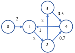
Figure 1: Network of four interconnected aircraft

The exosystem states are defined as $w=(r_{v},r_{\phi 1},r_{\phi 2},d_{\phi 1},d_{\phi 2})^{T}$, where $r_{v},r_{\phi 1},r_{\phi 2}$ are the states of the reference signal, and $d_{\phi 1},d_{\phi 2}$ denote the sensor noise in the channel of roll angle. The matrix $S$ is defined as follows:

$$S=\begin{bmatrix}0&0&0&0&0\\ 0&0&-\frac{2}{3}&0&-0.1\\ 0&\frac{1}{4}&0&0&0\\ 0&0&0&0&1\\ 0&0&0&-1&0\end{bmatrix}$$

The states of each aircraft are considered as $x_{i}=(v_{i},r_{ri},\phi_{i},y_{ri},T_{ai},T_{ri})^{T}$, the sideways velocity, roll rate, roll angle, yaw rate, and delays of the two commands, respectively. The measured output $y_{i}$ is considered as $y_{i}=(v_{i},\phi_{i})^{T}$, and $u_{i}=(\delta_{a_{c}i},\delta_{r_{c}i})^{T}$, the aileron deflection and rudder deflection commands. The regulated outputs $e_{i}$ are the tracking errors of sideways velocity and roll angle.

The state matrix of each aircraft for $i=1,\ldots,4$ is given as

$$A_{i}=\begin{bmatrix}-0.178&6.079&9.763&-65.623&0&2.890\\ -0.057&-3.810&0&1.343&-10.750&1.187\\ 0&1.000&0&0.094&0&0\\ 0.025&-0.062&0&-0.475&0.345&-2.220\\ 0&0&0&0&-11.111&0\\ 0&0&0&0&0&-11.111\end{bmatrix}$$

Also, for $i=1,\ldots,4$ we have

$$B_{i}= \begin{bmatrix}0&-2.8900\\ 10.7500&-1.1870\\ 0&0\\ -0.3450&2.2200\\ 22.2222&0\\ 0&22.2222\end{bmatrix},\ C_{y,i}=\begin{bmatrix}1&0&0&0&0&0\\ 0&0&1&0&0&0\end{bmatrix}$$

$$H_{e,i}= \begin{bmatrix}-1&0&0&0&0\\ 0&0&-1&0&0\end{bmatrix},\ H_{y,1}=\begin{bmatrix}1&-1&0&0&0\\ 1&-1&0&0&0\end{bmatrix}$$

Also $C_{y,i}=C_{e,i}$ and $H_{y,2}=H_{y,3}=H_{y,4}=0$. Conditions (A.1)-(A.6) may readily be checked to be valid; in solving (15)-(16) we used

$$\Gamma = \begin{bmatrix}-0.0045&-0.0877&0.0472&-0.0145&0.0327\\ 0.0112&-0.0427&-0.0139&-0.0065&0.0100\end{bmatrix}$$

$$\Pi = \begin{bmatrix}1.0000&0&0&0&0\\ 0.0002&0.2480&-0.0138&0.0000&-0.0866\\ 0&0&1.0000&0&0\\ -0.0022&0.0211&0.1467&-0.0002&-0.0076\\ -0.0089&-0.1773&0.0837&-0.0231&0.0659\\ 0.0223&-0.0847&-0.0329&-0.011&0.0203\end{bmatrix}$$

From the network graph in Figure 1, we see that the informed group of agents consists of agent 1, while agents 2, 3 and 4 are uninformed. The Laplacian matrix of the digraph is

$$\mathcal{L}=\begin{bmatrix}0&0&0&0&0\\ -2&3&0&0&-1\\ 0&-2&2&0&0\\ 0&0&-2&2&0\\ 0&0&-0.7&-0.5&1.2\end{bmatrix}$$

The distributed nature of the control scheme can be understood in terms of this aircraft example system. The controller design of the matrices required for the control scheme (17)-(19) for each aircraft can be done without knowing the identity (flight dynamics) of the other aircraft in the network, provided there is a consensus on the location of closed-loop poles. Regarding knowledge of the communication digraph $\mathcal{G}$, aircraft in the informed group need only know of those aircraft to whom they are directly linked by an edge of the digraph. Aircraft in the uninformed group require sufficient information to enable them to compute the Laplacian submatrix $\mathcal{L}_{33}$. The exosystem (2) represents a flight maneuver that all the aircraft are to execute. The maneuver involves varying the sideways velocity and roll angle of each aircraft. Global knowledge of the $S$ matrix defining the exosystem dynamics means that all aircraft are aware of the maneuver - the purpose of the control scheme presented in [6] is to enable all aircraft in the network to synchronise their execution of the maneuver with that of the leader aircraft.

The invariant zeros of each agent system $(A_{i},B_{i},C_{y,i})$ are at $\{-50.54,\ 11.11,\ 11.11\}$. Hence each system has one minimum phase zero at $-50.54$. There are 6 state variables, and two inputs and outputs. Thus (21) is satisfied, indicating that a search for feedback matrices to ensure the state feedback $\tilde{u}=F\tilde{x}$ yields a nonovershooting response on the nominal plant (20) is likely to succeed. It is also worth noting that the system is of nonminimum phase, due to the repeated right complex plane zero at $11.11$. [24] investigated the transient response of MIMO nonminimum phase systems, and found that, although overshoot could generally be avoided, doing so often came at the cost of undershoot, and vice-versa.

To investigate the application of the nonovershooting control method proposed in this paper, we assume that estimates of the initial states of each agent and the exosystem have been obtained as follows

$$x_{1,0} = \begin{bmatrix}-1&0&-1&1&0&0\end{bmatrix}^{T}$$

$$x_{2,0} = \begin{bmatrix}0&-1&-1&0&-1&-1\end{bmatrix}^{T}$$

$$x_{3,0} = \begin{bmatrix}-1&0&-1&1&0&-1\end{bmatrix}^{T}$$

$$x_{4,0} = \begin{bmatrix}-1&1&-1&1&0&-1\end{bmatrix}^{T}$$

$$w_{0} = \begin{bmatrix}1&1&0&0&0\end{bmatrix}^{T}$$

The NOUS toolbox [21] was used to seek such feedback matrices for the nominal system (20) of each agent, from initial conditions $\tilde{x}_{i,0}=x_{i,0}-\Pi w_{0}$. The toolbox asks the user to nominate a desired interval of the negative real line for the location of the closed-loop eigenvalues. We chose the interval $(-2.5,-.3)$, and in each case the search succeeded, yielding feedback matrices

$$F_{1} = \begin{bmatrix}0.006&0.025&-0.031&0.120&0.631&-0.250\\ 0.061&0.023&-0.354&1.08&1.38&-2.04\end{bmatrix}$$

$$F_{2} = \begin{bmatrix}0.005&0.015&-0.025&0.158&0.578&-0.250\\ 0.055&0.004&-0.387&1.29&1.39&-2.07\end{bmatrix}$$

$$F_{3} = \begin{bmatrix}0.00&-0.007&-0.086&0.485&0.646&-0.230\\ 0.004&-0.325&-0.978&5.056&1.61&-2.55\end{bmatrix}$$

$$F_{4} = \begin{bmatrix}0.004&0.029&0.041&0.136&0.506&-0.239\\ 0.056&0.049&-0.306&0.775&1.36&-2.00\end{bmatrix}$$

Figure 2 shows the tracking errors for the sideways velocity and roll angle for each agent, when the the control law $\tilde{u}_{i}=F_{i}\tilde{x}$ is applied to the nominal plant (20) with initial condition $\tilde{x}_{i,0}=x_{i,0}-\Pi_{i}w_{0}$. These yield nonovershooting tracking errors $\tilde{e}_{i}$ for both outputs of all agents. This situation corresponds to the tracking errors that would be observed from the multi-agent system (1) under the distributed dynamic output feedback controller (17)-(19) if there were no error in the estimates of the initial agent and exosystem states, and then $\bar{\epsilon}(0)=0$ and $\hat{\epsilon}(0)=0$.

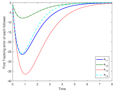
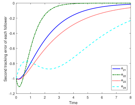
Figure 2: Tracking errors with no error in the initial state estimates

To implement the dynamic controller (17)-(19), we chose $\mu_{0}=-12$ and $\gamma=24$. These choices satisfy (24) as $\rho(S)$ lies on the imaginary axis, and $\rho(\mathcal{L}_{33})=\{1.2,\ 2,\ 2\}$. Observer gain matrices $L_{1,1}$, $L_{2,1}$ and $L_{i}$ for $i\in\{2,3,4\}$ to ensure the closed-loop matrices in (23) have spectrum lying to the left of $\mu_{0}$ were obtained using the MATLAB${}^{\textrm{\tiny{\textregistered}}}$ place command:

$$L_{11}=10^{6}\begin{bmatrix}-1.004&2.628\\ -0.020&0.051\\ -1.004&2.628\\ -0.153&0.401\\ -0.000&0.000\\ 0.000&-0.000\end{bmatrix},L_{21}=10^{7}\begin{bmatrix}0.593&-1.556\\ 0.492&-1.294\\ -0.108&0.284\\ 0.427&-1.109\\ 0.402&-1.058\end{bmatrix}$$

$$L_{2}=L_{3}=L_{4}=\begin{bmatrix}-32.5424&-3.1068\\ -1.8177&-147.3808\\ -0.1349&-27.7723\\ 3.7878&-17.6487\\ 0.1207&1.7550\\ -0.2203&0.4804\end{bmatrix}$$

To show the effect of the initial state estimate errors $\bar{\epsilon}(0)$ and $\hat{\epsilon}(0)$ in the system response, we shall assume these errors are 1% of the state estimates. Hence the initial states of systems (32) and (46) are

$$\bar{\xi}(0) = 1.01\bar{x}(0),\ \bar{\eta}(0)=1.01\bar{w}(0)$$

$$\hat{\xi}(0) = 1.01\hat{x}(0),\ \hat{\eta}(0)=1.01\hat{w}(0)$$

Figure 3 shows the tracking errors for the sideways velocity and roll angle for each agent, assuming these errors in the estimates of the initial states.

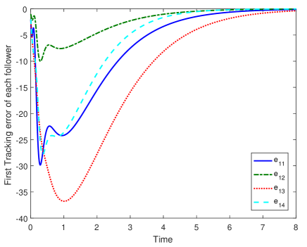
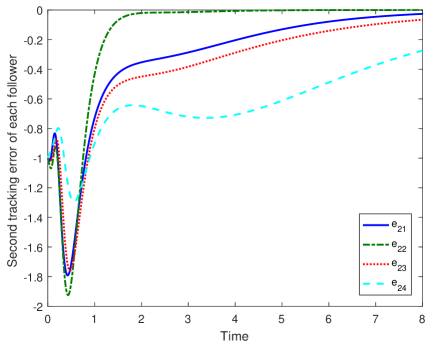
Figure 3: Tracking errors allowing for errors in the initial state estimates

We observe that both tracking errors from all four agents converge to zero without changing sign, and thus overshoot is avoided in both outputs of all four agents - a total of 8 outputs. If the dynamic controller (17)-(19) had been designed using the methods of [6] for the choice of the state feedback matrices, then the tracking errors would also converge to zero, however the transient responses of each output component would be expected to involve some overshoot, as may be observed in Figure 3 of [6]. Overshoot would occur even if the initial state estimation errors were zero [5].

The additional contribution of the control methods in [18] is to choose the feedback matrices in a manner that avoids overshoot and hence enables the transient period of the control action - during which synchronisation is being achieved and when the aircraft to do not yet all have the same sideways velocity - to be conducted in a smoother and potentially less dangerous manner.

VI Conclusion

We have investigated the problem of designing a consensus control scheme to solve the output regulation problem with a desirable transient response for a family of linear multi-agent systems. The distributed consensus output regulation scheme of Su and Huang was combined with the nonovershooting feedback control scheme of Schmid and Ntogramatzidis to achieve output regulation without overshoot for all agents, under Assumptions (A.1)-(A.8). The author’s believe this to be the first control methodology to achieve a nonovershooting transient response for MIMO multi-agent consensus problems.

Theorem IV.1 guarantees the existence of a neighbourhood of the estimated initial state $\tilde{x}_{i,0}$ such that, if the actual system initial state lies within this neighbourhood, then nonovershooting output regulation will be achieved by the distributed dynamic measurement output feedback controller in (17)-(19). Estimating the size of this neighbourhood is an open problem, however, the neighbourhood can be adjusted by the choice of $\lambda_{0}$, $\mu_{0}$ and $\gamma$ in (23)-(24). The neighbourhood becomes larger if the initial states of some agents are known, and also if the nonovershooting behaviour is only required in a selection of the agent outputs. In practice, the size of this neighbourhood can be estimated with the assistance of the NOUS MATLAB${}^{\textrm{\tiny{\textregistered}}}$ toolbox [21]. This toolbox allows the user to obtain state feedback matrices for a nonovershooting response from the estimated system initial state, for each agents. Combining these within (17)-(19) and simulating the response of (1) from a range of error estimates of the initial system state will enable this neighbourhood to be approximated.

VII Acknowledgements

The authors thank the Associate Editor and the anonymous reviewers for their extensive and insightful comments that have resulted in many improvements to the paper.

VIII Appendix

Proof of Lemma II.4: Assume firstly that $g(t)>0$ for all $t\geq 0$. Define $\lambda=\min\{\lambda_{i}:i\in\{1,\dots,m\}\}$. Then $\mu<\lambda$ by assumption. Define $f_{1}:\rightarrow$ with

$$f_{1}(t)=-\sum_{i=1}^{n}\ e^{\mu_{i}t}(|\alpha_{i}|+|\beta_{i}|)$$ (56)

Then $f_{1}(t)\leq f(t)$ for all $t\geq 0$. As $f_{1}$ and $g$ are the sums of finitely many negative real exponential functions, they have finitely many local extrema, and there exists a $\bar{t}>0$ such that both $f_{1}$ and $g$ are monotonic on the interval $t\geq\bar{t}$, and $f_{1}(t)\rightarrow 0$ and $g(t)\rightarrow 0$ as $t\rightarrow\infty$. Hence we have $\delta_{1}>0$ such that

$$\frac{1}{\delta_{1}}=\sup\left\{\frac{-f_{1}(t)}{g(t)}:0\leq t\leq\bar{t}\right\}$$ (57)

and so $0<g(t)+\delta_{1}f_{1}(t)$ for all $0\leq t\leq\tilde{t}$. Consider $t>\bar{t}$. As $f_{1}$ is a SEDS function with rate $\mu$, we know that for $t>\bar{t}$

$$-f_{1}(t)\leq|f_{1}(\bar{t})|e^{\mu(t-\bar{t})}$$ (58)

Assume without loss of generality that the $\{\lambda_{1},\dots,\lambda_{m}\}$ are ordered so that $\lambda_{1}<\lambda_{2}<\dots<\lambda_{m}$. Then $\beta_{m}e^{\lambda_{m}t}$ is the dominant term of $g$ as $t\rightarrow\infty$. Also the assumption that $g(t)>0$ for all $t\geq 0$ implies $\beta_{m}>0$. We next introduce the set of integers $T_{1}=\{i\in\{1,\dots,m\}:\beta_{i}\beta_{m}>0\}$ and the exponential function

$$g_{1}(t)=\sum_{i\in T_{1}}\ \beta_{i}e^{\lambda_{i}t}$$ (59)

Clearly $g_{1}(t)>0$ for all $t\geq 0$, and as $m\in T_{1}$, we see that $\beta_{m}e^{\lambda_{m}t}$ is the dominant term of $g_{1}$. Hence we can introduce the function $\gamma(t)$ such that $g(t)=\gamma(t)g_{1}(t)$. Then $0<\gamma(t)\leq 1$ for all $t\geq\bar{t}$, and $\gamma(t)\rightarrow 1$ as $t\rightarrow\infty$. Define $\gamma_{0}>0$ with $\gamma_{0}=\inf\{\gamma(t):t\geq\bar{t}\}$; we then have for all $t>\bar{t}$ that

$$g(t)\geq\gamma_{0}g_{1}(t)\geq\gamma_{0}g_{1}(\bar{t})e^{\lambda_{1}(t-\bar{t})}$$ (60)

From (58) and (60), we obtain for $t>\bar{t}$,

$$\frac{-f_{1}(t)}{g(t)} \leq \frac{|f_{1}(\bar{t})|e^{\mu(t-\bar{t})}}{\gamma_{0}g_{1}(\bar{t})e^{\lambda_{1}(t-\bar{t})}}$$ (61)

$$< \frac{|f_{1}(\bar{t})|}{\gamma_{0}g_{1}(\bar{t})}$$ (62)

as $\mu<\lambda_{1}$. Defining $\delta_{2}=\frac{\gamma_{0}g_{1}(\bar{t})}{|f_{1}(\bar{t})|}>0$, we obtain $0<g(t)+\delta_{2}f_{1}(t)$ for all $t>\bar{t}$. Finally choosing $\delta=\min\{\delta_{1},\delta_{2}\}$, and noting that $f_{1}(t)\leq f(t)$, we have $g(t)+\delta f(t)>0$ for all $t\geq 0$. A similar argument can be used if $g(t)<0$ for all $t\geq 0$, and the result follows.

References

• [1] A.ย Saberi, A.ย Stoorvogel and P.ย Sannuti, Control of linear systems with regulation and input constraints, ser. Communications and Control Engineering, Springer, 2000.
• [2] Y. Hong, L. Gao, D. Cheng, and J. Hu, Lyapunov-based approach to multiagent systems with switching jointly connected interconnection, IEEE Transactions on Automatic Control, 52 (2007) 943โ€“-948.
• [3] J. Xiang, W. Wei, and Y. Li, Synchronized output regulation of networked linear systems, IEEE Transactions on Automatic Control, 54, (2009) 1336โ€“-1341.
• [4] J. Huang, Remarks on synchronized output regulation of linear networked systems, IEEE Transactions on Automatic Control, 56 (2011) 630โ€“-631.
• [5] Y. Su and J. Huang, Cooperative Output Regulation of Linear Multi-Agent Systems, IEEE Transactions on Automatic Control, 57 (2012) 1062โ€“1066.
• [6] Y. Su and J. Huang, Cooperative output regulation of linear multi-agent systems by output feedback, Systems & Control Letters, 61 (2012) 1248โ€“1253.
• [7] Z. Gajic and M. Lelic, Modern Control Systems Engineering, London: Prentice Hall, 1996.
• [8] M. Sato, Robust model-following controller design for LTI systems affected by parametric uncertainties: a design example for aircraft motion, International Journal of Control 82 (4) (2009) 689โ€“704.
• [9] L. Yu, and J. Wang, Robust cooperative control for multi-agent systems via distributed output regulation. Systems & Control Letters, 62(11), (2013) 1049โ€“1056.
• [10] J. Ploeg, N. van de Wouw and H. Nijmeijer, $L_{p}$ String Stability of Cascaded Systems: Application to Vehicle Platooning. IEEE Transactions on Control Systems Technology, 22, (2014) 786โ€“793.
• [11] J. Monteil , M. Bouroche and D.J. Leith, $L_{2}$ and $L_{1}$ Stability Analysis of Heterogeneous Traffic With Application to Parameter Optimization for the Control of Automated Vehicles, accepted for publication in IEEE Transactions on Control Systems Technology 2018.
• [12] M.J. Park, O.M. Kwon and A. Seuret, Weighted Consensus Protocols Design based on Network Centrality for Multi-agent Systems with Sampled-data, IEEE Transactions on Automatic Control, 62 (2017) 2916 - 2922.
• [13] L. Macarella, Y. Karayiannidis and D.V. Dimarogonas, Multi-agent Second Order Average Consensus with Prescribed Transient Behavior, IEEE Transactions on Automatic Control, in press. DOI 10.1109/TAC.2016.2636749
• [14] C. Lei, W.Sun and J. Yeow, A Distributed Output Regulation Problem for Multi-agent Linear Systems with Application to Leader-follower Robotโ€™s Formation Control, Proceedings of the 35th Chinese Control Conference, Chengdu, 2016,
• [15] D. Martinec, I. Herman and M. Sebek, A travelling wave approach to a multi-agent system with a path-graph topology, Systems & Control Letters, 99 (2017) 90โ€“98.
• [16] S. Yang, J.X. Xu, X. Li, Iterative learning control with input sharing for multi-agent consensus tracking, Systems & Control Letters, 94 (2016) 97โ€“106.
• [17] G.S. Seyboth, W. Ren, F. Allgower, Cooperative control of linear multi-agent systems via distributed output regulation and transient synchronization, Automatica, 68 (2016) 132โ€“139.
• [18] R.ย Schmid, and L.ย Ntogramatzidis, A unified method for the design of nonovershooting linear multivariable state-feedback tracking controllers, Automatica, 46 (2010) 312โ€“321.
• [19] R.ย Schmid, and L.ย Ntogramatzidis, The design of nonovershooting and nonundershooting multivariable state feedback tracking controllers, Systems & Control Letters, 61 (2012) 714โ€“722.
• [20] R. Schmid, and L. Ntogramatzidis, Nonovershooting and nonundershooting exact output regulation, Systems & Control Letters, 70 (2014) 30โ€“37.
• [21] A.ย Pandey and R.ย Schmid, NOUS: a MATLAB${}^{\textrm{\tiny{\textregistered}}}$ toolbox for the design of nonovershooting and nonundershooting multivariable tracking controllers, Proceedings of the Second IEEE Australian Control Conference Sydney, 2012.
• [22] M. Mesbahi, and M. Egerstedt, Graph theoretic methods in multiagent networks, Princeton University Press, 2010.
• [23] B.C.ย Moore, On the Flexibility Offered by State Feedback in Multivariable systems Beyond Closed Loop Eigenvalue Assignment, IEEE Transactions on Automatic Control, 21, (1976) 689โ€“692.
• [24] R. Schmid and A. Pandey, The role of nonminimum phase zeros in the transient response of multivariable systems, Proceedings of the 50th IEEE Conference on Decision and Control Orlando, 2011.