Optimizing active work: Dynamical phase transitions, collective motion, and jamming

Abstract

Active work measures how far the local self-forcing of active particles translates into real motion. Using Population Monte Carlo methods, we investigate large deviations in the active work for repulsive active Brownian disks. Minimizing the active work generically results in dynamical arrest; in contrast, despite the lack of aligning interactions, trajectories of high active work correspond to a collectively moving, aligned state. We use heuristic and analytic arguments to explain the origin of dynamical phase transitions separating the arrested, typical, and aligned regimes.

I Introduction

Active particles constitute an important class of non-equilibrium systems, with examples ranging from bacteria to synthetic colloidal swimmers Berg2008book ; Cates2012RPP ; Howse2007PRL ; Theurkauff2012PRL ; Palacci2013Science ; Bricard2013Nature ; BechingerRMP . These particles expend energy to propel themselves, driving active matter out of equilibrium at microscopic scales and causing rich dynamical behaviors. Some of these are universal, whereby systems that differ microscopically show similar emergent physics Marchetti:2013:RMP , such as motility induced phase separation (MIPS) Cates:2015:ARCMP ; Tailleur:2008:PRL ; FilyYaouenMarchettiCristina ; RednerHaganBaskaran ; Bialke:2013:EPL ; Wysocki:2014:EPL ; Stenhammar:2014:SM , collective motion Vicsek1995PRL ; Gregoire2004PRL ; Ballerini2008PNAS ; Vicsek2012PhysRep ; Solon2015PRLflock ; Deseigne2010PRL ; Bricard2013Nature ; Deseigne2010PRL , lane formation Klymko2016 ; Junco2018 or motile defects Narayan2007Science ; Sanchez2012Nature ; Giomi2013PRL ; Thampi2014EPL ; Decamp2015Nature ; Mahault2018arXiv .

Many recent advances in our understanding of non-equilibrium systems are based on large-deviation theory (LDT) Derrida2007JSM ; Touchette_LD . This extends the counting procedures of equilibrium statistical mechanics from configuration space to trajectory space, addressing collective phenomena such as dynamical phase transitions. It has been used to characterize dynamical symmetries Gallavotti1995PRL ; Kurchan1998JPA ; Lebowitz1999 ; Crooks1999PRE , measure free energy differences Jarzynski1997PRL ; Collin2005Nature , and locate atypical trajectories, such as activated processes Kohn2005JNS . LDT has proven useful in fields ranging from dynamical systems Tailleur2007NatPhys and glasses Garrahan2007PRL ; hedges_dynamic_2009 to fluid mechanics Grafke2015JPA and geophysical flows Bouchet2014FDR . In contrast, the full range of insights offered by LDT to active matter remains largely unexplored, despite a handful of pioneering studies Thompson2011JSM ; PhysRevLett.119.158002 ; whitelam2017phase ; Chaudhuri2014PRE ; Ganguly2013PRE ; mandal2017entropy ; shankar2018hidden .

Here we use LDT to study active Brownian particles (ABPs) interacting via repulsive central forces. We focus on the large deviations of the active work, defined as the particle-averaged inner product of propulsive force and velocity. This measures how far the local self-forcing of active particles translates into real motion. A recent study PhysRevLett.119.158002 used brute-force simulations to sample the fluctuations of active work in a dilute system of active dumbbells and found a low active work to correlate with the emergence of ordered clusters in this system. Here we use an advanced numerical method Giardina_Kurchan_Peliti ; Tailleur2007NatPhys ; Hurtado2009PRL ; Giardina2011JSP ; Nemoto_Bouchet_Jack_Lecomte ; Nemoto_Jack_Lecomte ; ray2017exact ; klymko2018rare ; Brewer_Clark_Bradford_Jack to explore the full large-deviation regime in all relevant regions of the phase diagram of our ABP model. We first show that finite systems always admit a large deviation principle, notwithstanding PhysRevLett.119.158002 , but that they are flanked by two dynamical phase transitions. Indeed, minimizing the active work always leads to complete dynamical arrest, whether or not the unbiased system exhibits MIPS. Biasing instead towards high active work, we find a striking result: trajectories now correspond to flocked states of aligned collective motion, despite the microscopic absence of aligning interactions. We explain the origin of the dynamical phase transitions separating these regimes using a combination of arguments including macroscopic fluctuation theory Bertini2002JSP ; Jack2015PRL .

II Model

We consider $N$ active Brownian particles interacting via purely repulsive pairwise forces in two spatial dimensions FilyYaouenMarchettiCristina ; RednerHaganBaskaran ; Stenhammar:2014:SM ; Wysocki:2014:EPL ; Bialke:2013:EPL . The positions and orientations of the particles are $\bm{r}_{i}$ and $\theta_{i}$; they evolve as

$$\dot{{\bm{r}}}_{i} =\mu{\bm{F}}_{i,\rm ex}+v_{\rm p}{{\bm{u}}}(\theta_{i})+\sqrt{2D}{\bm{\eta}}_{i}\;;\quad\dot{\theta_{i}}=\sqrt{2D_{\rm r}}\xi_{i}\;,$$ (1)

where ${{\bm{\eta}}}_{i},\xi_{i}$ are zero-mean unit-variance Gaussian white noises, $\mu$ is a particle’s mobility, $v_{\rm p}$ its bare self-propulsion speed and ${{\bm{u}}}(\theta_{i})=(\cos\theta_{i},\sin\theta_{i})$ its orientation vector, and $D,D_{r}$ are translational and rotational diffusivities. Particles interact via a repulsive WCA potential, detailed in Appendix A, of range $\sigma$. For consistency with RednerHaganBaskaran , we set $D_{r}=3D/\sigma^{2}$ and the WCA strength parameter to be $D/\mu$. Then, we choose space and time units such that $\sigma=1$ and $\sigma/v_{\rm p}=1$ (see Appendix A). When the persistence length $\ell_{\rm p}\equiv v_{\rm p}/D_{\rm r}$ is much larger than the particle size, $\ell_{\rm p}/\sigma\gtrsim 15$, the system undergoes MIPS: at high volume fractions, a vapor of motile particles coexists with dense macroscopic clusters FilyYaouenMarchettiCristina ; RednerHaganBaskaran ; Wysocki:2014:EPL ; Stenhammar:2014:SM ; Bialke:2013:EPL . For smaller $\ell_{\rm p}$, the system remains uniform and the main effect of activity is to enhance the effective translational diffusivity.

For interacting particles, a natural measure of how efficiently active forces create motion is given by the propulsive speed $v_{i}\equiv\dot{{\bm{r}}_{i}}\cdot{{\bm{u}}(\theta_{i})}$ which projects a particle’s velocity along its orientation. This relates directly to the active work PhysRevLett.119.158002 , the total work done by the active forces on the particles, which obeys (in the Stratonovich convention)

$$W_{\rm a}(t)\equiv\frac{v_{\rm p}}{\mu}\int_{0}^{t}\sum_{i=1}^{N}\dot{{\bm{r}}}_{i}(\tau)\cdot{{\bm{u}}}\big{(}\theta_{i}(\tau)\big{)}\,\mathrm{d}\tau=\sum_{i=1}^{N}\int_{0}^{t}\frac{v_{\rm p}v_{i}(\tau)}{\mu}\,\mathrm{d}\tau.$$ (2)

For conservative interactions, $W_{\rm a}$ relates to the dissipation in the thermostat $\int dt\dot{{\bm{r}}}_{i}\cdot(\dot{{\bm{r}}}_{i}-\sqrt{2D}{{\bm{\eta}}}_{i})$ Sekimoto1997 ; Toyabe2010 ; Seifert2012 ; Kanazawa2014 ; Ahmed2016 , and thus to the entropy production in the full $\{r_{i},\theta_{i}\}$ configuration space PhysRevLett.119.158002 . (This is generally distinct from that measured in position space $\{r_{i}\}$ PhysRevLett.117.038103 . See also Puglisi2017 ; marconi2017heat for a comparative study of different entropy productions.) It is convenient to consider a normalized rate of active work per particle, $w\equiv W_{\rm a}\mu/(v_{p}^{2}Nt)$. The dilute limit of vanishing packing fraction $\phi\to 0$ then leads to $\langle w\rangle=1$ which serves as a useful reference point.

For fixed $N$ and large $t$, the distribution of $w$ has a large-deviation form

$$p(w)\sim\exp[-tI(w)]\;,$$ (3)

where $I(w)$ is a rate function Touchette_LD . The corresponding cumulant generating function (CGF)

$$G(s)=\lim_{t\rightarrow\infty}\frac{1}{t}\log\left\langle e^{-stNw}\right\rangle\;$$ (4)

is related to $I(w)$ by Legendre transformation. As shown in Appendix B, the functions $I(w)$ and $G(s)$ are convex, and $G(s)$ obeys a fluctuation relation $G(s)=G(a-s)$, with $a=3\ell_{p}/\sigma$. The CGF is analogous to a free energy in equilibrium statistical mechanics lecomte2007thermodynamic ; Touchette_LD ; garrahan_first-order_2009 ; chetrite2013nonequilibrium . Within this analogy, trajectories of our two-dimensional system (evolving in time) correspond to configurations of an anisotropic three-dimensional system. Suppose that one spatial dimension (the “length”) of this anisotropic system becomes infinite, while the others remain fixed – this is analogous to considering trajectories with $t\to\infty$ and fixed $N$. Phase transitions are not possible in such one-dimensional geometries, which is another way to see that $G(s)$ must be convex (and analytic).

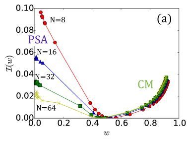
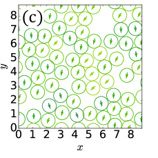
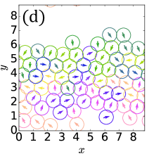
Figure 1: (a) The rescaled rate function ${\cal I}(w)$, for system parameters where MIPS occurs ($\phi=0.65$, $\ell_{p}=40\sigma$). The $N$-dependence shows strong finite size effects for $w<\langle w\rangle$. The labels PSA and CM indicate respectively regimes of phase-separated arrest and collective motion. (b) The function $w(s)$ exhibits two sharp crossovers, which we attribute to two dynamical phase transitions. (These appear in (a) as near-linear segments of the rate function.) (c,d) Snapshot configurations for $N=64$ in the biased ensemble, corresponding to the arrested phase ($s=0.8$, (d)) and the collective motion phase ($s=-3.2$, ${(c)}$). Particles are colored according to their orientations. For corresponding movies see Suppl .

Now consider the limit $N\to\infty$ (taken at fixed $\phi$, after $t\to\infty$). In this case dynamical phase transitions are possible – the analogous thermodynamic system is becoming infinite along more than one spatial dimension garrahan_first-order_2009 ; jack2010large ; Nemoto_Jack_Lecomte . The dynamical analogues of the (bulk) thermodynamic free-energy and entropy are

$${\cal I}(w)=I(w)/N\qquad\text{and}\qquad{\cal G}(s)=G(s)/N\;.$$ (5)

As in statistical mechanics, singularities in the large-$N$ limits of these functions are interpreted as phase transitions bodineau2005 ; bertini2005 ; garrahan_first-order_2009 ; jack2010large ; Nemoto_Jack_Lecomte ; vaik2014 .

To observe and measure large deviations of the active work, we use a cloning algorithm Tailleur2007NatPhys ; Giardina2011JSP ; Nemoto_Bouchet_Jack_Lecomte , also known as Population Monte Carlo delmoral , whose optimised implementation using modified dynamics Nemoto_Bouchet_Jack_Lecomte is detailed in Appendix C. (See Giardina_Kurchan_Peliti ; Brewer_Clark_Bradford_Jack for a lattice version of this algorithm, and whitelam2017phase for a recent application to active systems.) In essence, the method relies on evolving a large population of copies of the system to generate “biased ensembles” of trajectories that sample the average in (4) with a cost that scales linearly in $t$, allowing direct access to the large-$t$ limit. For positive and negative $s$, the biased ensembles are dominated by trajectories with atypically small and large $w$ respectively.

III results

We first consider a system whose parameters lie (as $N\to\infty$) within the MIPS region, $\ell_{p}=40\sigma$ and $\phi=0.65$ (See RednerHaganBaskaran for the full phase diagram of the system). We compute ${\cal G}(s)$, and $w(s)\equiv-{\cal G}^{\prime}(s)$, which is the mean value of the active work in the presence of the bias, and its inverse $s(w)$. We also determine the rescaled rate function as ${\cal I}(w)=-s(w)w-{\cal G}(s(w))$. Our numerical results (Fig. 1) show three regimes separated by dynamical phase transitions that we discuss below: a MIPS-like coexistence between vapor and dense phases near $s=0$; a phase-separated arrest (PSA) at large positive $s$; and a collectively moving (CM) state at large negative $s$.

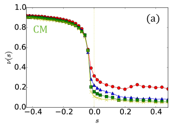
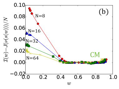
Figure 2: (a) The orientation vector $\nu(s)$ in the biased ensemble. (b) The difference between the two quantities appearing in (7), showing saturation of this bound at $w>\langle w\rangle_{0}$.

III.1 Large active work: Collective motion

For large negative $s$, the biased ensemble probes atypically large values of the active work. Despite the absence of aligning interactions, the biased ensemble is dominated by trajectories where particles’ orientations are aligned with each other, and they move collectively as a flock. A global order parameter for this transition is the orientation

$$\hat{\nu}=\bigg{|}\frac{1}{N}\sum_{i=1}^{N}{{\bm{u}}}(\theta_{i})\bigg{|},\qquad\nu(s)=\langle\hat{\nu}\rangle_{s}\,,$$ (6)

where angle brackets are averages within the biased ensemble. Fig. 2 shows the emergence of global orientation for $s<0$. In contrast, in the unbiased case ($s=0$) there is no emergent alignment: $\nu(s=0)\to 0$ at large $N$.

To understand the emergence of order, note that particle alignment naturally promotes active work: the CM state has far fewer collisions than if motion is incoherent, so that active forces translate more efficiently into particle motion. To confirm this interpretation, we compute the rate function $J(\bar{\nu})$ of the time-integrated orientation $\bar{\nu}=t^{-1}\int_{0}^{t}\hat{\nu}(\tau)\mathrm{d}\tau$ whose probability distribution scales as $p(\bar{\nu})\sim{\rm e}^{-tJ(\bar{\nu})}$, analogous to (3). Since the orientational dynamics of ABPs is independent of their positions, the rate function $J$ can be computed semi-analytically as shown in Appendices E and F. It measures the probability of rare events where rotational symmetry is spontaneously violated. Now, define $I_{2}$ as the joint rate function for $\bar{\nu}$ and $w$, and let $\nu_{*}(w)=\nu(s(w))$ be the average global orientation for a biased system with active work $w$. Then $I(w)=\inf_{\nu}I_{2}(w,\nu)=I_{2}(w,\nu_{*}(w))$ where the first equality is the contraction principle for large deviations Touchette_LD and the second follows because the infimum is achieved by $\nu_{*}$. Similarly $J(\nu_{*}(w))=\inf_{w^{\prime}}I_{2}(w^{\prime},\nu_{*}(w))\leq I_{2}(w,\nu_{*}(w))$ and hence

$${\cal I}(w)\geq\frac{J(\nu_{*}(w))}{N}.$$ (7)

Fig. 2(b) shows that the inequality (7) is almost saturated when $w>\langle w\rangle_{0}$. Physically, this indicates that the probability cost for creating a large fluctuation of the active work is dominated, for $s<0$, by the cost to create an improbable global orientation, with an associated spontaneous symmetry breaking and an accompanying singularity in ${\cal I}(w)$. It appears that “the best strategy” for a set of active particles to move fast is for them to collectively align. Here “best” means least improbable within the microscopic stochastic dynamics specified by (1). Note that the emergence of macroscopic arrested clusters due to MIPS can be suppressed by local torques that limit the head-on collisions of particles pohl2014dynamic ; matas2014hydrodynamic ; zottl2014hydrodynamics . It is thus quite remarkable that the most likely way to generate an efficient motion of each particle, and hence a large active work, is through the emergence of a collectively moving state, and not through such local rearrangements (which do not lead to a CM state).

III.2 Small active work: Dynamic arrest

For positive $s$, the biased ensemble selects trajectories with atypically low active work, so that propulsive effort leads to little motion. On increasing the bias, we find the system sharply transitions into a dynamically arrested state. (See Fig 1c and movies in Suppl ). A signature of this transition is the discontinuity in $w(s)$ reported in Fig 1(b), which signifies a first-order dynamical phase transition: the linear segment in ${\cal I}(w)$, for $w<0.5$, is analogous to a Maxwell construction and the discontinuity in $w(s)$ to a jump in the order parameter. These features should become strict singularities only as $N\to\infty$ but are clearly visible for $N=32,64$. (Note however that $G(s)$ and $I(w)$ are well-defined for any finite $N$, notwithstanding PhysRevLett.119.158002 .) As $N$ increases, the critical value of $s$ moves towards zero (see Appendix G for this finite-size scaling analysis), suggesting that bulk MIPS states live on the verge of a first order transition to complete arrest.

This situation is reminiscent of dynamical phase transitions arising for activity-biased kinetically constrained models (KCMs) of glassy systems Garrahan2007PRL ; garrahan_first-order_2009 . Indeed, our findings for $s>0$ can be qualitatively understood by generalizing arguments developed for KCMs. Specifically, we exploit a variational principle that allows the rate function $I(w)$ to be computed by considering what auxiliary ‘control’ forces need to be added to a system to realise the rare trajectories of interest Nemoto2011 ; TouchetteJSM2015 ; JackSollichEPJ2015 . Stabilizing a large, dense cluster in a system undergoing MIPS only requires applying forces on its boundaries, hence involving a sub-extensive number of particles. This argument, detailed in Appendix H, immediately leads to $\lim_{N\to\infty}{\cal I}(w)=0$ and a dynamical phase transition at $s=0$. Since the argument is variational in nature, it can be exploited in numerical simulations: we have used it to obtain bounds on $I(w)$ for $w<\langle w\rangle$ in large systems as shown in Appendix H, which are consistent with the presence of a phase transition and complement the accurate results for $I(w)$ in small systems that we show in Fig. 1.

III.3 Large deviations for homogeneous steady states

So far we considered systems with parameters for which the unbiased, large $N$ dynamics shows steady-state MIPS. We now consider large deviations from a steady state that is homogeneous. We focus on two state points: $(\phi,\ell_{p})=(0.1,40\sigma)$, corresponding to a reduced density but large $\ell_{p}$, and $(\phi,\ell_{p})=(0.65,6.7\sigma)$, corresponding to high density but smaller $\ell_{p}$. Fig. 3 and movies in Suppl show the asymptotic phases observed for large positive and negative $s$ to be similar in both cases: for $s<0$, they again exhibit collective motion while for $s>0$ the system undergoes phase-separated arrest. Compared to Fig. 1, the crossover to the PSA state in Fig. 3c is smoother; at this smaller value of $\ell_{p}$, the density fluctuations of the ABPs are smaller (there is no MIPS) and the instability to phase separation is weaker.

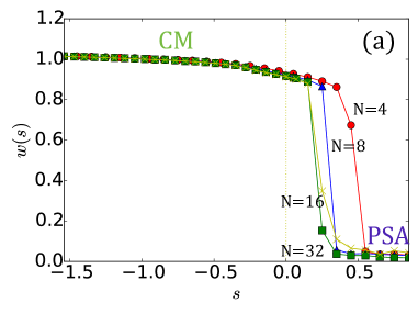
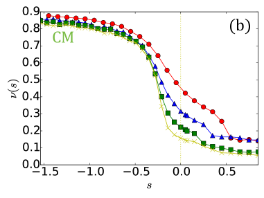
Figure 3: The active work $w(s)$ and the orientation $\nu(s)$ for two state points where the unbiased dynamic gives homogeneous steady states. In (a,b) the state point is $(\phi,\ell_{p})=(0.1,40\sigma)$; in (c,d) it is $(\phi,\ell_{p})=(0.65,6.7\sigma)$. The crossovers shown in these figures separate the homogeneous fluid ($s=0$) from a CM phase ($s<0$) and a PSA state ($s>0$). These phases are qualitatively similar to those shown in Fig 1(c,d). See movies in Suppl .

This bias-induced phase separation can be explained by a hydrodynamic argument Jack2015PRL . For a macroscopically homogeneous fluid, long-wavelength density fluctuations should obey an equation of the form Bertini2015

$$\dot{\rho}=\nabla\cdot\left(D_{\rm eff}(\rho)\nabla\rho+\sqrt{2\sigma(\rho)}\xi\right)$$ (8)

where $\rho$ is the local density, $D_{\rm eff}$ is a (density-dependent) diffusivity, $\sigma(\rho)$ is a noise strength, and $\xi$ is a Gaussian white noise. (Higher-order gradients, while relevant to MIPS wittkowski2014Ncom ; nardini2017PRX ; solon2018PRE ; tjhung2018arxiv , are negligible for the long-wavelength fluctuations of interest here.) It is then natural to approximate $W[\rho]\simeq\frac{v_{\rm p}}{\mu}\int dtdx\rho v(\rho)$, where $v(\rho)$ is the average of the effective active speed $v_{i}$ in a homogeneous system of density $\rho$. This $v(\rho)$ is known to decrease linearly with density in pairwise-force active particles FilyYaouenMarchettiCristina so that the active work density $\kappa(\rho)\equiv\frac{v_{\rm p}}{\mu}\rho v(\rho)$ is a concave function. A density fluctuation $\delta\rho$ then leads to a fluctuation of the active work $\delta W=\int\frac{1}{2}\kappa^{\prime\prime}(\rho)(\delta\rho)^{2}\mathrm{d}x$ with $\kappa^{\prime\prime}(\rho)<0$.

Large deviations of such observables in the setting of (8) are known to lead to phase separation in the large system limit $L\to\infty$ whenever $s>0$ and $\kappa^{\prime\prime}(\rho)<0$ Jack2015PRL : a long-wavelength linear instability arises for $s>\lambda_{c}/L^{2}$ with $\lambda_{c}=(2\pi D_{\rm eff})^{2}/|\sigma\kappa^{\prime\prime}|$ Appert2008 ; Lecomte2012 ; Jack2015PRL . This bias-induced instability arises in passive systems Lecomte2012 ; Jack2015PRL , and we argue that it applies to homogeneous, isotropic active fluids also, since the form of (8) is the same. Alongside it, any conventional phase separation, including MIPS, creates an instability even in the unbiased case, $s=0$. This sets in as $D_{\rm eff}(\rho)\to 0$. In that limit, $\lambda_{c}\to 0$ so that the bias-induced and motility-induced instabilities merge; physically, the bias reinforces the natural tendency to phase separate. (The convergence with $N$ is slowest in the small persistence length region, Fig. 3c, which is furthest from the MIPS regime.) In contrast, the collective motion regime observed for $s<0$ has no passive counterpart and cannot be captured by (8), which assumes that the orientations are only weakly affected by the bias, and can therefore be integrated out.

IV Conclusion

We have shown, using a combination of numerical simulations and theoretical arguments, that active systems interacting via pairwise forces undergo several different dynamical phase transitions. Choosing a bias field to select trajectories of low active work, we found these trajectories to involve a coexistence of a dense jammed, arrested domain with a dilute vapor. This is the most likely way in which an active system that is normally a uniform bulk fluid can stop moving. Biasing in the other direction to find trajectories of high active work, we found collective motion with aligned propulsion directions despite the absence of aligning interactions microscopically.

We end by speculating about a link between large deviations and evolutionary biology, motivated by two observations. First, the cloning algorithm involves the evolution of a population of systems: the method balances their natural dynamics (which favour the unbiased steady state) and a selection pressure, which favours systems with atypical values of some fitness function (here, active work) brotto2016population ; brotto2017model . Second, we have shown that alignment among ABPs tends to suppress collisions, leading to efficient motion. We have argued that alignment is an effective strategy for promoting particle motion, with a minimal cost (in probability). We suggest that this cost-minimisation strategy might also be viewed as a possible evolutionary strategy for maximising active work in biological systems. We do not expect a general correspondence between evolutionary strategies and cost minimisation, particularly since cost-minimisation strategies may be complicated, perhaps requiring concerted motion across large length scales jack2010large ; Nemoto2011 ; chetrite2013nonequilibrium . However, one may imagine that some robust characteristics (such as global alignment) might appear generically in both cost-minimisation strategies and evolutionary strategies.

Appendix A Non-dimensionalized time evolution equations and Peclet number

We use the particle radius $\sigma$ and propulsion speed $v_{\rm p}$ to define dimensionless position and time as ${\bm{r}}_{i}/\sigma$ and $v_{\rm p}t/\sigma$. We also define a dimensionless mobility $\alpha=D/(D_{\rm r}\sigma^{2})$. The dynamics (1) then become

$$\dot{{\bm{r}}}_{i} = \alpha\frac{\sigma}{\ell_{\rm p}}\tilde{{\bm{F}}}_{i,\rm ex}+{{\bm{u}}}_{i}(\theta_{i})+\sqrt{\alpha\frac{2\sigma}{\ell_{\rm p}}}{\bm{\eta}}_{i},$$ (9)

$$\dot{\theta_{i}} = \sqrt{\frac{2\sigma}{\ell_{\rm p}}}\xi_{i}.$$ (10)

The interaction force $\tilde{{\bm{F}}}_{i,\rm ex}$ stems from the (dimensionless) WCA potential

$$V_{\rm ex}=\big{[}4\big{(}(1/r)^{12}-(1/r)^{6}\big{)}+1\Big{]}\Theta(2^{1/6}-r)$$ (11)

where $\Theta$ is a Heaviside step function. (Following RednerHaganBaskaran , we chose the typical strength of the WCA potential to be $D/\mu$ in the original units.) The Peclet number $\rm Pe$ used in RednerHaganBaskaran is given as

$${\rm Pe}=\frac{\ell_{p}}{\sigma\alpha}$$ (12)

with $\alpha=1/3$. The normalized active work rate is $w(t)=(1/(Nt))\sum_{i=1}^{N}\int_{0}^{t}d\tilde{t}\ \dot{{\bm{r}}}_{i}(\tilde{t})\cdot{{\bm{u}}}_{i}$ in the dimensionless position and time units.

Appendix B Fluctuation relation, and convexity of $I(w)$

The large deviation function of the active work satisfies the fluctuation theorem

$${\cal G}(s)={\cal G}({\rm Pe}-s).$$ (13)

This means that ${\cal G}(s)$ takes its minimum value at $s_{\rm min}={\rm Pe}/2$, where ${\cal G}^{\prime}(s)$ vanishes. In Fig. 4, we show a numerical example of ${\cal G}(s)$ for ${\rm Pe}=1$ which illustrates this symmetry property.

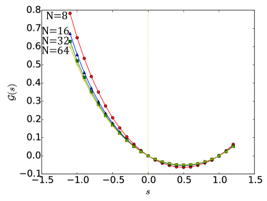
Figure 4: For ${\rm Pe}=1$ and $\phi=0.65$, the cumulant generating function ${\cal G}(s)$ is symmetric around $s_{\rm min}=1/2$, as predicted by Eq. (13).

We now derive Eq. (13). First, let $P(\Omega)$ be the probability density of a trajectory $\Omega=({\bm{r}}_{i}(t^{\prime}),\theta_{i}(t^{\prime}))$ with $t^{\prime}\in[0,t]$. We then define a time-reversed trajectory as $\Omega^{T}=({\bm{r}}_{i}(t-t^{\prime}),\theta_{i}(t-t^{\prime}))$. Using standard methods PhysRevLett.117.038103 , the ratio between $P(\Omega)$ and $P(\Omega^{T})$ can be computed as

$$\frac{P(\Omega)}{P(\Omega^{T})}=\exp\left\{{\rm Pe}\ tNw(t)-V(t)+V(0)\right\}$$ (14)

where $V(t)$ is the total potential energy of the system at time $t$. Multiplying both sides by $e^{-stNw}P(\Omega^{T})$ and summing upon all possible $\Omega$, we get

$$\left\langle e^{-stNw}\right\rangle=\left\langle e^{(s-{\rm Pe})tNw-V(0)+V(t)}\right\rangle.$$ (15)

The large time limit then immediately leads to the fluctuation theorem (13).

An additional question within large-deviation theory is whether the limit in (4) is finite, and whether the resulting $G(s)$ is analytic. This discussion refers to finite systems, since it is clear from our results that the large-$N$ limit of ${\cal G}(s)$ can develop singularities. If $G(s)$ is differentiable everywhere then $I(w)$ can be obtained from it by Legendre transformation and is also convex and continuous: all this follows from the Gärtner-Ellis theorem Touchette_LD . The finite-size scaling in our numerical work assumes that this theorem is applicable.

As noted in Sec 3.2 of Chetrite2015 , $G(s)$ is the largest eigenvalue of a differential operator (which is called the tilted generator); and if this operator satisfies conditions for a Perron-Frobenius theorem then it has a finite spectral gap. This is sufficient to establish that $G(s)$ is analytic, and hence the Gärtner-Ellis theorem. The Perron-Frobenius theorem can be applied to systems such as (1) as long as the number of particles is finite, the domain in which they move is compact, the noise terms in (1) are additive (and non-zero), and the forces are bounded.

For the system considered here, there is one subtlety, which is that the interparticle forces $\bm{F}_{i,\rm ex}$ in (1) are not bounded. This prevents direct application of the Perron-Frobenius theorem. From a mathematical point of view, this raises the possibility that large deviations might be realised by trajectories where two (or more) particles collapse onto the same point. We do not have a mathematical proof that such trajectories can be neglected, but we see no physical reason why they would be relevant, and there is no evidence for them in our numerical computations. For this reason, we argue that the unbounded interaction forces in (1) can be truncated when particles come very close to the same point, without changing any of the behaviour that we find. In such a modified system (with finite $N$), the Perron-Frobenius theorem applies, which means that $G(s)$ and hence $I(w)$ are both analytic, and are related by Legendre transformation

Appendix C Enhanced convergence of the cloning algorithm using modified dynamics

Our cloning algorithm gives access to the cumulant generating function ${\cal G}(s)$ in the limit of large number of clones. To enhance the convergence of the algorithm, a generic strategy is to rely on modified dynamics Nemoto_Bouchet_Jack_Lecomte . We now detail the implementation of this strategy to sample the large deviations of the active work in our model. We first introduce the following modification of dynamics (1):

$$\dot{{\bm{r}}}_{i}=\alpha\frac{\sigma}{\ell_{\rm p}}\tilde{{\bm{F}}}_{i,\rm ex}+(1+f){{\bm{u}}}_{i}(\theta_{i})+\sqrt{\alpha\frac{2\sigma}{\ell_{\rm p}}}{\bm{\eta}}_{i},$$ (16)

and

$$\dot{\theta_{i}}=\sqrt{\frac{2\sigma}{\ell_{\rm p}}}\xi_{i}.$$ (17)

We denote $P_{f}(\Omega)$ the probability of $\Omega$ in this new system. The following identity is then satisfied:

$$P(\Omega)e^{-stNw}=P_{f}(\Omega)e^{-stN\tilde{w}},$$ (18)

where the new bias $\tilde{w}$ is defined as

$$\begin{split}-stN\tilde{w}=&-\left(s+\frac{f{\rm Pe}}{2}\right)tNw\\ &+\sum_{i=1}^{N}\int_{0}^{t}d\tilde{t}\left(\frac{f{\rm Pe}}{2}+\frac{f^{2}{\rm Pe}}{4}+\frac{f}{2}\tilde{{\bm{F}}}_{i,\rm ex}\cdot{{\bm{u}}}_{i}\right).\end{split}$$ (19)

Simulating dynamics (16) and (17) with the bias (19) is thus equivalent to simulating (1) with a bias $-stNw$. In practice we use $f=-2s/{\rm Pe}$ so that the new bias $\tilde{w}$ reduces to

$$\tilde{w}=1-\frac{s}{\rm Pe}+\frac{1}{tN\rm Pe}\sum_{i=1}^{N}\int_{0}^{t}d\tilde{t}\tilde{{\bm{F}}}_{i,\rm ex}\cdot{{\bm{u}}}_{i}.$$ (20)

which indeed produced faster convergence with the number of clones used in the simulations.

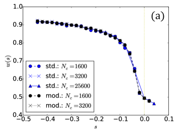
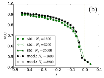
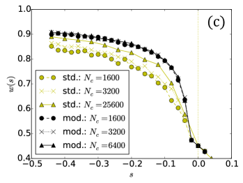
Figure 5: The estimator of the active work obtained from the standard (std.) cloning algorithm (left-hand side of Eq.(26)) and modified (mod.) cloning algorithm (right-hand side of Eq.(26)) for $N=16$ (a), $N=32$ (b) and $N=64$ (c). The modified algorithm shows a much faster convergence as the number of clones is increased. Its limiting value agrees with the standard algorithm when the latter has converged.

To characterize the CM state, we add another modifying force described as follows:

$$\dot{{\bm{r}}}_{i}=\frac{1}{{\rm Pe}}{\bm{F}}_{i,\rm ex}+\left(1-\frac{2s}{\rm Pe}\right){{\bm{u}}}(\theta_{i})+\sqrt{\frac{2}{\rm Pe}}{\bm{\eta}}_{i},$$ (21)

and

$$\dot{\theta_{i}}=-gN\frac{\partial}{\partial\theta_{i}}\hat{\nu}^{2}+\sqrt{\frac{2}{\alpha{\rm Pe}}}\xi_{i},$$ (22)

where $g$ is a parameter whose value is discussed later. Similarly, the probability of the trajectory $\omega$ in this modified system, $P_{\rm mod}$, is given by

$$\begin{split}&P_{\rm mod}(\omega)\propto\exp\Bigg{\{}-\frac{\rm Pe}{4}\int dt\sum_{i}\bigg{(}\dot{{\bm{r}}}_{i}-\frac{1}{\rm Pe}{\bm{F}}_{i,\rm ex}-\\ &\left(1-\frac{2s}{\rm Pe}\right){{\bm{u}}}(\theta_{i})\bigg{)}^{2}-\frac{\alpha\rm Pe}{4}\int dt\sum_{i}\left(\dot{\theta}_{i}+gN\frac{\partial}{\partial\theta_{i}}\hat{\nu}^{2}\right)^{2}\\ &-\frac{1}{4\rm Pe}\int dt\sum_{i}\frac{\partial}{\partial{{\bm{r}}}_{i}}{\bm{F}}_{i,\rm ex}+\frac{1}{2}\int_{0}^{\tau}dt\sum_{i}gN\frac{\partial^{2}\hat{\nu}^{2}}{\partial\theta_{i}^{2}}\bigg{\}}.\end{split}$$ (23)

By taking the ratio between $P(\omega)$ and $P_{\rm mod}(\omega)$, we get

$$\begin{split}&\frac{P_{\rm mod}(\omega)}{P(\omega)}\simeq\exp\Bigg{\{}-s\tau Nw+\int_{0}^{\tau}dt\bigg{[}sN-\frac{s^{2}}{\rm Pe}N\\ &+\frac{s}{\rm Pe}\sum_{i}{\bm{u}}_{i}\cdot{\bm{F}}_{i,\rm ex}+g-gN\hat{\nu}^{2}-\frac{g^{2}\alpha\rm Pe}{\hat{\nu}^{2}}\sum_{i}\sin^{2}(\theta_{i}-\varphi)\bigg{]}\Bigg{\}},\end{split}$$ (24)

where $w$ is the active work introduced in the main text. By defining the modified active work $w_{\rm mod}$ as

$$\begin{split}&w_{\rm mod}=\frac{1}{\tau}\int_{0}^{\tau}dt\bigg{[}1-\frac{s}{\rm Pe}+\frac{1}{N\rm Pe}\sum_{i}{\bm{u}}_{i}\cdot{\bm{F}}_{i,\rm ex}+\frac{g}{sN}\\ &-\frac{g}{s}\hat{\nu}^{2}-\frac{g^{2}\alpha\rm Pe}{sN\hat{\nu}^{2}}\sum_{i}\sin^{2}(\theta_{i}-\varphi)\bigg{]}\end{split}$$ (25)

we thus get

$$P(\omega)e^{-s\tau Nw}=P_{\rm mod}(\omega)e^{-s\tau Nw_{\rm mod}}.$$ (26)

Note that $g$ is a free parameter here: the equality (26) holds irrespective of the value of $g$.

As discussed in Nemoto_Bouchet_Jack_Lecomte and in Appendix H, there is an optimal modification to the dynamics – if this could be found, then the cloning algorithm would have zero error and $w_{\rm mod}$ in (26) would become a simple number (independent of the trajectory), equal to $-G(s)/s$. However, finding the optimal modification is as difficult as solving the large-deviation problem analytically, and is out of reach for most problems, including this one. Hence, the modifying forces used here are not optimal in the sense of Nemoto_Bouchet_Jack_Lecomte but we may still choose $g$ so as to enfore the following equality:

$$\left\langle-sw_{\rm mod}\right\rangle_{\rm mod}=\hat{G}(s),$$ (27)

where $\left\langle\ \right\rangle_{\rm mod}$ means the average in the modified dynamics (obtained from the cloning algorithm) and $\hat{G}(s)$ is the estimator of the cumulant generating function within the cloning algorithm. We found that this is an efficient way to choose our modifying force.

In Fig. 5, we compare the standard cloning algorithm (left-hand side of Eq.(27)) and the modified one (right-hand side of Eq.(27)) by plotting the active work as a function of s. We see that for $N=16$ and $N=32$, both algorithm lead to the same function $w(s)$, but that the modified dynamics converges much faster as the number of clones $N_{c}$ increases. For $N=64$, however, the standard algorithm shows a very slow convergence, unlike our modified algorithm.

Appendix D The parameters used for Population Monte-Carlo method

Here we summarize the parameters used to get the results in the main text. Convergence is obtained using the number of clones $N_{c}=25600$. The time-step of the simulations is $dt=0.001$; cloning steps are performed each $\Delta t=0.01$. The simulation length varies from $t=30000$ to $300000$, depending on the values of $N$ and $s$. We checked the convergence with respect to the cloning parameters $N_{c}$, $\delta t$, $t$, for all values of $s$ except for the immediate vicinity of the PSA transition point ($s>0$). Around this transition point, we observe a slight unphysical concavity of ${\cal G}(s)$ which is a signature that perfect convergence is out of reach of our simulations (see Fig. 7(a)).

Appendix E Derivation of the polarization dynamics

This appendix is devoted to the derivation of the dynamics of the stochastic polarization $\hat{\nu}$ defined in Eq. (6) of the main text. It can be written as

$$\hat{\nu}=\frac{1}{N}\sqrt{\sum_{\{i,j\}=1}^{N}\cos(\theta_{i}-\theta_{j})}.$$ (28)

We introduce a global phase $\varphi$ such as

$$\hat{\nu}e^{\varphi}\equiv\frac{1}{N}\sum_{j=1}^{N}e^{\text{i}\theta_{j}}.$$ (29)

Using Itô’s lemma, taking time derivative of Eq. (28) gives

$$\dot{\hat{\nu}} =-\frac{\sqrt{2D_{\text{r}}}}{N^{2}\hat{\nu}}\sum_{\{i,j\}=1}^{N}\xi_{i}\sin(\theta_{i}-\theta_{j})$$ (30)

$$\quad+\frac{D_{\text{r}}}{N}\sum_{k=1}^{N}\frac{d^{2}}{d\theta_{k}^{2}}\sqrt{\sum_{\{i,j\}=1}^{N}\cos(\theta_{i}-\theta_{j})},$$

where we have used $\dot{\theta}_{i}=\sqrt{2D_{\text{r}}}\xi_{i}$, and $\xi_{i}$ is a zero-mean unit-variance Gaussian white noise. The second term can be written as

$$\sum_{k=1}^{N}\frac{d^{2}}{d\theta_{k}^{2}}\sqrt{\sum_{\{i,j\}=1}^{N}\cos(\theta_{i}-\theta_{j})} =-\sum_{\{k,l\}=1}^{N}\frac{d}{d\theta_{k}}\frac{\sin(\theta_{k}-\theta_{l})}{\sqrt{\sum_{i,j}\cos(\theta_{i}-\theta_{j})}}$$ (31)

$$=\frac{N-\sum_{k,l}\cos(\theta_{k}-\theta_{l})}{\sqrt{\sum_{i,j}\cos(\theta_{i}-\theta_{j})}}-\sum_{\{k,l,m\}=1}^{N}\frac{\sin(\theta_{k}-\theta_{l})\sin(\theta_{k}-\theta_{m})}{\big{[}\sum_{i,j}\cos(\theta_{i}-\theta_{j})\big{]}^{3/2}}$$

$$=\frac{1}{\hat{\nu}}-N\hat{\nu}-\frac{1}{(N\hat{\nu})^{3}}\sum_{\{k,l,m\}=1}^{N}\sin(\theta_{k}-\theta_{l})\sin(\theta_{k}-\theta_{m}).$$

The noise term appearing in (30) is denoted by

$$\Lambda\equiv\sum_{\{i,j\}=1}^{N}\xi_{i}\sin(\theta_{i}-\theta_{j}).$$ (32)

It is a zero-mean Gaussian white noise with correlations

$$\langle\Lambda(t)\Lambda(0)\rangle =\sum_{\{i,j,k,l\}=1}^{N}\langle\xi_{i}(t)\xi_{k}(0)\rangle\sin[\theta_{i}(t)-\theta_{j}(t)]$$ (33)

$$\qquad\qquad\times\sin[\theta_{k}(0)-\theta_{l}(0)]$$

$$=\delta(t)\sum_{\{j,k,l\}=1}^{N}\sin(\theta_{k}-\theta_{j})\sin(\theta_{k}-\theta_{l}).$$

To proceed further, we note that the sum can be simplified, using (29), as

$$\sum_{\{j,k,l\}=1}^{N} \sin(\theta_{k}-\theta_{j})\sin(\theta_{k}-\theta_{l})$$ (34)

$$=(N\hat{\nu})^{2}\sum_{i=1}^{N}\sin(\theta_{i}-\varphi)^{2}$$

$$=(N\hat{\nu})^{2}\int_{0}^{2\pi}\sin(\theta-\varphi)^{2}\psi(\theta,t)d\theta,$$

where we have introduced the angular distribution $\psi(\theta,t)\equiv\sum_{i}\delta[\theta-\theta_{i}(t)]$. We now assume that $\psi$ is close to uniform, which should hold for $\hat{\nu}\ll 1$ and large $N$, to obtain

$$\sum_{\{j,k,l\}=1}^{N}\sin(\theta_{k}-\theta_{j})\sin(\theta_{k}-\theta_{l})$$ (35)

$$\quad\xrightarrow[\hat{\nu}\ll 1,~{}N\gg 1]{}\frac{N^{3}\hat{\nu}^{2}}{2\pi}\int_{0}^{2\pi}\sin(\theta-\varphi)^{2}d\theta=\frac{N^{3}\hat{\nu}^{2}}{2}.$$

Finally, substituting this result in (31) and (33), then (30) reduces to

$$\frac{d\hat{\nu}}{dt}=D_{\rm r}\left[\frac{1}{2N\hat{\nu}}-\hat{\nu}\right]+\sqrt{\frac{D_{\rm r}}{N}}\xi.$$ (36)

which is a closed (autonomous) equation for the evolution of $\hat{\nu}$.

Appendix F CGF of the time-averaged total orientation $\bar{\nu}$

In this appendix, we consider the cumulant generating function of $\bar{\nu}$, defined as

$${\cal H}(\varsigma)=\frac{1}{N}\lim_{t\rightarrow\infty}\frac{1}{t}\log\left\langle e^{-tN\varsigma\bar{\nu}}\right\rangle\;.$$ (37)

We work under the assumption that $\hat{\nu}\ll 1$, $N\rightarrow\infty$ so that we can use the time-evolution equation for $\hat{\nu}$ given by (36). We introduce the rescaled variable $q=\hat{\nu}\sqrt{N}$, whose dynamics is given by

$$\frac{dq}{dt}=D_{\rm r}\left[\frac{1}{2q}-q\right]+\sqrt{D_{\rm r}}\xi\;.$$ (38)

Note that (38) is independent of $N$. We then consider the cumulant generating function of the time-averaged value of $q$:

$$f(k)=\lim_{t\rightarrow\infty}\frac{1}{t}\log\left\langle e^{-k\int_{0}^{t}d\tilde{t}q(\tilde{t})}\right\rangle\;.$$ (39)

The CGF $f(k)$ is the largest eigenvalue of the following operator:

$$L_{k}[\cdot]=-\frac{\partial}{\partial q}\left[D_{r}\left(\frac{1}{2q}-q\right)\cdot\right]+\frac{D_{\rm r}}{2}\frac{\partial^{2}}{\partial q^{2}}\left[\cdot\right]-kq.$$ (40)

Since $L_{k}$ is independent of $N$, $f(k)$ is a well-defined smooth function in the $N\rightarrow\infty$ limit:

$$f(k)=\lim_{N,t\rightarrow\infty}\frac{1}{t}\log\left\langle e^{-k\int d\tilde{t}q(\tilde{t})}\right\rangle.$$ (41)

Using $k=\varsigma\sqrt{N}$, ${\cal H}(\varsigma)$ can now be expressed as

$${\cal H}(\varsigma)=\frac{f(\varsigma\sqrt{N})}{N},$$ (42)

or, conversely,

$$f(k)=N{\cal H}\left(\frac{k}{\sqrt{N}}\right).$$ (43)

In Fig. 6, we numerically demonstrate (43). To do so, we compare the results obtained by applying the cloning algorithm to the dynamics (10) of $N$ independent rotors, which yields the right-hand side of (43)), with the result of the numerical diagonalization of the operator (40), which yields the left-hand side of (43). The results of the cloning algorithm for several $N$ clearly collapse onto a single function $f(k)$. Note that this overlap is satisfied not only for positive $s$ (where the assumption $\hat{\nu}\ll 1$ is safely satisfied) but also for negative $s$ close to the origin.

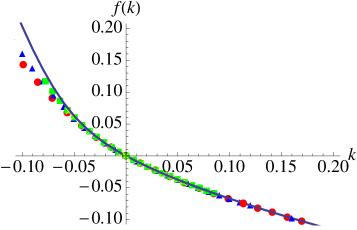
Figure 6: An example of $f(k)$ obtained from numerical diagonalization of the operator (40) in blue solid line. We set $D_{\rm r}=1/40$. We also plot $N{\cal H}(k/\sqrt{N})$ obtained from the application of the cloning algorithm to $N$ active rotors. The data points for $N=8,16,32,64$ correspond to red-circle, blue-triangle green-square and yellow cross. We can see clear overlap of the data points to a single line, demonstrating the validity of (43).

Appendix G Finite-size scaling to estimate PSA transition point in $N\rightarrow\infty$

We denote by $s_{c}(N)$ the PSA transition point for finite system size $N$. It is defined as the value of $s$ that maximizes the second derivative of ${\cal G}(s)$ for positive $s$. The obstacle to estimate $s_{c}(N)$ is that there are strong finite-size effects with respect to the number of clones $N_{c}$ around $s_{c}(N)$ (that artificially violate the convexity of ${\cal G}(s)$ as seen in Fig. 7(a)). To overcome this difficulty, we extract $s_{c}(N)$ from the crossing point of the straight lines obtained by fitting the data for $s<s_{c}(N)$ and $s_{c}(N)<s$, as shown in Fig. 7(a). Due to the convexity of $G(s)$, the crossing point determined in this way gives a good approximation of $s_{c}(N)$ Nemoto_Jack_Lecomte . We then plot $s_{c}(N)$ as a function of $N$ and extrapolate $\lim_{N\rightarrow\infty}s_{c}(N)$. As seen from Fig. 7(b), $s_{c}(N)$ is consistent with a convergence to zero, with a power law: $s_{c}(N)\sim N^{-a}$.

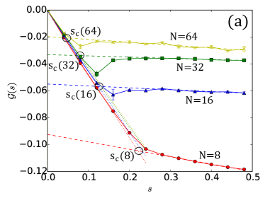
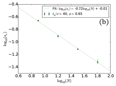
Figure 7: (a) How to estimate $s_{c}(N)$ from ${\cal G}(s)$. For $s$ slightly larger than $s_{c}$, the required number of clones $N_{c}$ needed to observe the convergence of the cloning algorithm rapidly increases beyond what can be reached numerically. As a consequence, we see an artificial violation of the concavity of ${\cal G}(s)$. To interpolate the correct shape of ${\cal G}(s)$, and locate $s_{c}(N)$, we use the data where the concavity is not violated. In both panels, dashed and dotted straight lines are obtained by fitting the data in inactive ($s\gg s_{c}(N)$) and active ($s\ll s_{c}(N)$) regions, respectively. Assuming a sharp kink Nemoto_Jack_Lecomte , we obtain the estimated value of $s_{c}(N)$ as the crossing point of these two lines (indicated as the black circles for each $N$). (b) $s_{c}(N)$ estimated from the finite-size scaling on the data up to $N=64$ (for $\ell_{\rm p}=40\sigma$, $\phi=0.65$) shows a power law decay with respect to $N$: $s_{c}(N)\sim N^{-a}$ with a positive constant $a$. In particular, this implies $\lim_{N\rightarrow\infty}s_{c}(N)=0$.

Appendix H Optimal control argument for dynamical arrest of a MIPS cluster (PSA transition)

We consider a system that is obtained by adding additional “control” forces to (1), leading to

$$\dot{{\bm{r}}}_{i} =B^{r}_{i}({{\bm{r}}},\theta)+\mu{\bm{F}}_{i,\rm ex}+v_{\rm p}{{\bm{u}}}(\theta_{i})+\sqrt{2D}{\bm{\eta}}_{i},$$

$$\dot{\theta_{i}} =B^{\theta}_{i}({{\bm{r}}},\theta)+\sqrt{2D_{\rm r}}\xi_{i}.$$ (44)

The control forces $B^{r},B^{\theta}$ depend on the co-ordinates of all particles. A general result in large-deviation theory (see, e.g., Eq. (54) of TouchetteJSM2015 as well as Nemoto2011 and the discussion in Sec. 4 of JackSollichEPJ2015 ) is that

$$I(w)=\inf_{B^{r},B^{\theta}\colon\langle w\rangle_{\rm control}=w}\Phi(B^{r},B^{\theta}),$$ (45)

where $\Phi$ is a “cost function”, and the infimum runs over those forces for which the steady state of (44) has a mean active work $w$. The cost function $\Phi$ is the relative entropy between two ensembles of trajectories, which are the (unbiased) steady state of the original system, and the steady state of the controlled system. This relative entropy is related to the large-deviation rate function at level-2.5: in the present context it is simply (TouchetteJSM2015, , Eq. (76))

$$\Phi(B^{r},B^{\theta})=\left\langle\sum_{i}\left[\frac{(B_{i}^{r})^{2}}{4D}+\frac{(B_{i}^{\theta})^{2}}{4D_{r}}\right]\right\rangle_{\rm control},$$ (46)

where the average is taken in the steady state of (44).

From (45) one has that for any control forces $B$ that realise the desired active work, then $I(w)\leq\Phi(B^{r},B^{\theta})$. To establish the existence of a phase transition at $s=0$, it is sufficient to find (for each $N$) some $B$ that realise the desired active work, with $\lim_{N\to\infty}N^{-1}\Phi(B^{r},B^{\theta})=0$ (that is, $\Phi$ is subextensive). In this case ${\cal I}_{\infty}(w)\equiv\lim_{N\to\infty}N^{-1}I(w)\leq\lim_{N\to\infty}N^{-1}\Phi(B^{r},B^{\theta})=0$. The rate function is non-negative so this is sufficient to show that ${\cal I}_{\infty}(w)=0$.

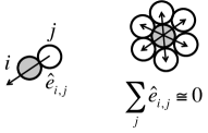
Figure 8: Schematic figure to show $\sum_{j}\hat{{\bm{e}}}_{i,j}\simeq 0$ when a particle (indicated as gray color) is surrounded by six particles.

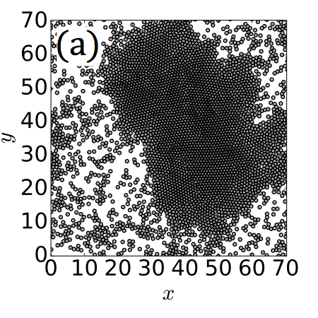
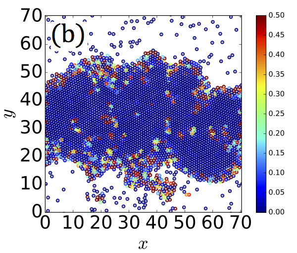
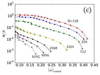
Figure 9: (a) Snapshot of the original dynamics, for $N=4096$ particles, leading to $\langle w\rangle\simeq 0.25$. (b) Snapshot of the dynamics with the control torque (47) and $g=0.22$. The control torques clearly reduce the number of particles in the gas phase, leading to a lower active work $\langle w\rangle\simeq 0.05$. The color code corresponds to the contribution of each particle to the cost function (46), normalized by $g^{2}$. The cost is clearly dominated by the subextensive contribution of the particles localized at the boundary of the main cluster. (c) The upper bound $\Phi$ of the large deviation function as a function of $\langle w\rangle_{g}=\left\langle w\right\rangle_{\rm control}$, normalized by the number of particles. The bound decreases as the system size increases.

To illustrate how this argument works, recall the case of kinetically constrained models. In that case the variational principle (45) simplifies JackSollichEPJ2015 , because the controlled systems are at equilibrium and are fully characterised by their Boltzmann distributions. One may then find $B$ such that the system is localised in a single state and the corresponding $\Phi$ is the escape rate from that site. In KCMs there are configurations for which this escape rate is subextensive, leading to ${\cal I}_{\infty}(a)=0$ for $0<a<\langle a\rangle$, (where $a$ is the dynamical activity).

In the present context, we suppose that the natural state of the system is phase-separated (due to MIPS) and we consider a controlled steady state that is also phase-separated. We take $B^{r}=0$, and we apply torques $B^{\theta}$ that act on the particles near the boundary of the dense cluster, which favour orientations pointing towards the cluster. These torques will help to reinforce the MIPS state, and they also act to compress the cluster, so that its density will increase, which tends to reduce particle motion. For any control force of this type, the only terms which contribute in (46) are from particles on the cluster boundary, so the number of such terms is subextensive. Hence $\Phi$ is subextensive (assuming that the $B^{\theta}_{i}$ are bounded). This means that ${\cal I}_{\infty}(w)=0$ for any value of the active work that can be realised by a perturbation of this type. Our data (Fig. 1) indicate that values of $w$ close to zero can be achieved with a subextensive cost, just as happens in KCMs.

Building such control forces and torques explicitly, that would apply only to particles located at the boundary of the cluster, is a numerical challenge. We can nevertheless test our hypothesis by considering the following protocol

$$B_{i}^{\theta}=-g\frac{\partial}{\partial\theta_{i}}\sum_{j}\hat{{\bm{e}}}_{i,j}\cdot{\bm{u}}_{i}(\theta_{i})$$ (47)

(with $B_{i}^{r}=0$). Here, $g>0$ is a constant parameter and $\hat{{\bm{e}}}_{i,j}$ is a unit vector from the particle $j$ to the particle $i$ when they interact and zero otherwise: $\hat{{\bm{e}}}_{i,j}=\Theta(2^{1/6}-r_{i,j}){\bm{r}}_{i,j}/r_{i,j}$ with ${\bm{r}}_{i,j}\equiv{\bm{r}}_{i}-{\bm{r}}_{j}$. The torques (47) will favor head-on collisions between interacting particles. At the boundary of the cluster, such torques lower the tendency of particles to rotate and leave the cluster. It will play little role in the gas phase, where there are few collisions. For the particles inside the dense arrested clusters, $B_{i}$ is also small by symmetry (see Fig. 8). Therefore, we expect that the dynamics with the control torque (47) will lead to a reinforcement of MIPS and hence a lower active work, with a cost function $(B_{i}^{\theta})^{2}/4D$ nearly vanishing outside the boundaries of the cluster.

Simulations using the control force (47) indeed show reduced numbers of gas-phase particles in Fig 9(a,b), leading to smaller values of the active work when compared to the original dynamics. Fig 9(c) shows that, furthermore, as the system sizes are increased, the upper bound of the LDF $\Phi(w)$ strongly decreases. These numerical results support our theory because they illustrate how a phase-separated arrested state can indeed be stabilised using a cost that is dominated by boundary contributions. Note that for much larger sizes, however, our cost function might saturate because the torque $B_{i}^{\theta}$ does not vanish exactly in the bulk of the cluster and gas phases. Only a protocol that would be exactly restricted to the boundary region could be used to achieve the $N\to\infty$ limit, which is anyway far beyond what we can do numerically.

References

- (1) Howard C Berg. E. coli in Motion. Springer Science & Business Media 2008.
- (2) Michael E Cates. Diffusive transport without detailed balance in motile bacteria: does microbiology need statistical physics? Reports on Progress in Physics 75, 042601 (2012).
- (3) Jonathan R. Howse, Richard A. L. Jones, Anthony J. Ryan, Tim Gough, Reza Vafabakhsh, and Ramin Golestanian. Self-Motile Colloidal Particles: From Directed Propulsion to Random Walk. Phys. Rev. Lett. 99, 048102 (2007).
- (4) I. Theurkauff, C. Cottin-Bizonne, J. Palacci, C. Ybert, and L. Bocquet. Dynamic Clustering in Active Colloidal Suspensions with Chemical Signaling. Phys. Rev. Lett. 108, 268303 (2012).
- (5) Jeremie Palacci, Stefano Sacanna, Asher Preska Steinberg, David J. Pine, and Paul M. Chaikin. Living Crystals of Light-Activated Colloidal Surfers. Science 339, 936 (2013).
- (6) Antoine Bricard, Jean-Baptiste Caussin, Nicolas Desreumaux, Olivier Dauchot, and Denis Bartolo. Emergence of macroscopic directed motion in populations of motile colloids. Nature 503, 95 (2013).
- (7) Clemens Bechinger, Roberto Di Leonardo, Hartmut Löwen, Charles Reichhardt, Giorgio Volpe, and Giovanni Volpe. Active particles in complex and crowded environments. Rev. Mod. Phys. 88, 045006 (2016).
- (8) M. C. Marchetti, J. F. Joanny, S. Ramaswamy, T. B. Liverpool, J. Prost, Madan Rao, and R. Aditi Simha. Hydrodynamics of soft active matter. Rev. Mod. Phys. 85, 1143 (2013).
- (9) Michael E. Cates and Julien Tailleur. Motility-Induced Phase Separation. Annual Review of Condensed Matter Physics 6, 219 (2015).
- (10) J. Tailleur and M. E. Cates. Statistical Mechanics of Interacting Run-and-Tumble Bacteria. Phys. Rev. Lett. 100, 218103 (2008).
- (11) Yaouen Fily and M. Cristina Marchetti. Athermal Phase Separation of Self-Propelled Particles with No Alignment. Phys. Rev. Lett. 108, 235702 (2012).
- (12) Gabriel S. Redner, Michael F. Hagan, and Aparna Baskaran. Structure and Dynamics of a Phase-Separating Active Colloidal Fluid. Phys. Rev. Lett. 110, 055701 (2013).
- (13) Julian Bialké, Hartmut Löwen, and Thomas Speck. Microscopic theory for the phase separation of self-propelled repulsive disks. EPL (Europhysics Letters) 103, 30008 (2013).
- (14) Adam Wysocki, Roland G Winkler, and Gerhard Gompper. Cooperative motion of active Brownian spheres in three-dimensional dense suspensions. EPL (Europhysics Letters) 105, 48004 (2014).
- (15) Joakim Stenhammar, Davide Marenduzzo, Rosalind J Allen, and Michael E Cates. Phase behaviour of active Brownian particles: the role of dimensionality. Soft Matter 10, 1489 (2014).
- (16) Tamás Vicsek, András Czirók, Eshel Ben-Jacob, Inon Cohen, and Ofer Shochet. Novel Type of Phase Transition in a System of Self-Driven Particles. Phys. Rev. Lett. 75, 1226 (1995).
- (17) Guillaume Grégoire and Hugues Chaté. Onset of Collective and Cohesive Motion. Phys. Rev. Lett. 92, 025702 (2004).
- (18) Michele Ballerini, Nicola Cabibbo, Raphael Candelier, Andrea Cavagna, Evaristo Cisbani, Irene Giardina, Vivien Lecomte, Alberto Orlandi, Giorgio Parisi, Andrea Procaccini, et al. Interaction ruling animal collective behavior depends on topological rather than metric distance: Evidence from a field study. Proceedings of the national academy of sciences 105, 1232 (2008).
- (19) Tamás Vicsek and Anna Zafeiris. Collective motion. Physics Reports 517, 71 (2012).
- (20) Alexandre P. Solon, Hugues Chaté, and Julien Tailleur. From Phase to Microphase Separation in Flocking Models: The Essential Role of Nonequilibrium Fluctuations. Phys. Rev. Lett. 114, 068101 (2015).
- (21) Julien Deseigne, Olivier Dauchot, and Hugues Chaté. Collective Motion of Vibrated Polar Disks. Phys. Rev. Lett. 105, 098001 (2010).
- (22) Katherine Klymko, Phillip L. Geissler, and Stephen Whitelam. Microscopic origin and macroscopic implications of lane formation in mixtures of oppositely driven particles. Phys. Rev. E 94, 022608 (2016).
- (23) Clara del Junco, Laura Tociu, and Suriyanarayanan Vaikuntanathan. Energy dissipation and fluctuations in a driven liquid. Proceedings of the National Academy of Sciences 115, 3569 (2018).
- (24) Vijay Narayan, Sriram Ramaswamy, and Narayanan Menon. Long-lived giant number fluctuations in a swarming granular nematic. Science 317, 105 (2007).
- (25) Tim Sanchez, Daniel TN Chen, Stephen J DeCamp, Michael Heymann, and Zvonimir Dogic. Spontaneous motion in hierarchically assembled active matter. Nature 491, 431 (2012).
- (26) Luca Giomi, Mark J. Bowick, Xu Ma, and M. Cristina Marchetti. Defect Annihilation and Proliferation in Active Nematics. Phys. Rev. Lett. 110, 228101 (2013).
- (27) Sumesh P Thampi, Ramin Golestanian, and Julia M Yeomans. Instabilities and topological defects in active nematics. EPL (Europhysics Letters) 105, 18001 (2014).
- (28) Stephen J DeCamp, Gabriel S Redner, Aparna Baskaran, Michael F Hagan, and Zvonimir Dogic. Orientational order of motile defects in active nematics. Nature materials 14, 1110 (2015).
- (29) B. Mahault, X.-c. Jiang, E. Bertin, Y.-q. Ma, A. Patelli, X.-q. Shi, and H. Chaté. Self-Propelled Particles with Velocity Reversals and Ferromagnetic Alignment: Active Matter Class with Second-Order Transition to Quasi-Long-Range Polar Order. Phys. Rev. Lett. 120, 258002 (2018).
- (30) Bernard Derrida. Non-equilibrium steady states: fluctuations and large deviations of the density and of the current. Journal of Statistical Mechanics: Theory and Experiment 2007, P07023 (2007).
- (31) Hugo Touchette. The large deviation approach to statistical mechanics. Physics Reports 478, 1 (2009).
- (32) G. Gallavotti and E. G. D. Cohen. Dynamical Ensembles in Nonequilibrium Statistical Mechanics. Phys. Rev. Lett. 74, 2694 (1995).
- (33) Jorge Kurchan. Fluctuation theorem for stochastic dynamics. Journal of Physics A: Mathematical and General 31, 3719 (1998).
- (34) Joel L. Lebowitz and Herbert Spohn. A Gallavotti–Cohen-Type Symmetry in the Large Deviation Functional for Stochastic Dynamics. Journal of Statistical Physics 95, 333 (1999).
- (35) Gavin E. Crooks. Entropy production fluctuation theorem and the nonequilibrium work relation for free energy differences. Phys. Rev. E 60, 2721 (1999).
- (36) C. Jarzynski. Nonequilibrium Equality for Free Energy Differences. Phys. Rev. Lett. 78, 2690 (1997).
- (37) Delphine Collin, Felix Ritort, Christopher Jarzynski, Steven B Smith, Ignacio Tinoco Jr, and Carlos Bustamante. Verification of the Crooks fluctuation theorem and recovery of RNA folding free energies. Nature 437, 231 (2005).
- (38) Robert V Kohn, Maria G Reznikoff, and Eric Vanden-Eijnden. Magnetic elements at finite temperature and large deviation theory. Journal of nonlinear science 15, 223 (2005).
- (39) Julien Tailleur and Jorge Kurchan. Probing rare physical trajectories with Lyapunov weighted dynamics. Nature Physics 3, 203 (2007).
- (40) Juan P. Garrahan, Robert L. Jack, Vivien Lecomte, Estelle Pitard, Kristina van Duijvendijk, and Frédéric van Wijland. Dynamical First-Order Phase Transition in Kinetically Constrained Models of Glasses. Physical Review Letters 98, 195702 (2007).
- (41) Lester O. Hedges, Robert L. Jack, Juan P. Garrahan, and David Chandler. Dynamic Order-Disorder in Atomistic Models of Structural Glass Formers. Science 323, 1309 (2009).
- (42) Tobias Grafke, Rainer Grauer, and Tobias Schäfer. The instanton method and its numerical implementation in fluid mechanics. Journal of Physics A: Mathematical and Theoretical 48, 333001 (2015).
- (43) F Bouchet, C Nardini, and T Tangarife. Stochastic averaging, large deviations and random transitions for the dynamics of 2D and geostrophic turbulent vortices. Fluid Dynamics Research 46, 061416 (2014).
- (44) Alasdair G Thompson, Julien Tailleur, Michael E Cates, and Richard A Blythe. Lattice models of nonequilibrium bacterial dynamics. Journal of Statistical Mechanics: Theory and Experiment 2011, P02029 (2011).
- (45) F. Cagnetta, F. Corberi, G. Gonnella, and A. Suma. Large Fluctuations and Dynamic Phase Transition in a System of Self-Propelled Particles. Phys. Rev. Lett. 119, 158002 (2017).
- (46) Stephen Whitelam, Katherine Klymko, and Dibyendu Mandal. Phase separation and large deviations of lattice active matter. The Journal of Chemical Physics 148, 154902 (2018).
- (47) Debasish Chaudhuri. Active Brownian particles: Entropy production and fluctuation response. Phys. Rev. E 90, 022131 (2014).
- (48) Chandrima Ganguly and Debasish Chaudhuri. Stochastic thermodynamics of active Brownian particles. Phys. Rev. E 88, 032102 (2013).
- (49) Dibyendu Mandal, Katherine Klymko, and Michael R. DeWeese. Entropy Production and Fluctuation Theorems for Active Matter. Phys. Rev. Lett. 119, 258001 (2017).
- (50) Suraj Shankar and M. Cristina Marchetti. Hidden entropy production and work fluctuations in an ideal active gas. Phys. Rev. E 98, 020604 (2018).
- (51) Cristian Giardinà, Jorge Kurchan, and Luca Peliti. Direct Evaluation of Large-Deviation Functions. Phys. Rev. Lett. 96, 120603 (2006).
- (52) Pablo I. Hurtado and Pedro L. Garrido. Test of the Additivity Principle for Current Fluctuations in a Model of Heat Conduction. Phys. Rev. Lett. 102, 250601 (2009).
- (53) Cristian Giardina, Jorge Kurchan, Vivien Lecomte, and Julien Tailleur. Simulating rare events in dynamical processes. Journal of statistical physics 145, 787 (2011).
- (54) Takahiro Nemoto, Freddy Bouchet, Robert L. Jack, and Vivien Lecomte. Population-dynamics method with a multicanonical feedback control. Phys. Rev. E 93, 062123 (2016).
- (55) Takahiro Nemoto, Robert L. Jack, and Vivien Lecomte. Finite-Size Scaling of a First-Order Dynamical Phase Transition: Adaptive Population Dynamics and an Effective Model. Phys. Rev. Lett. 118, 115702 (2017).
- (56) Ushnish Ray, Garnet Kin-Lic Chan, and David T. Limmer. Exact Fluctuations of Nonequilibrium Steady States from Approximate Auxiliary Dynamics. Phys. Rev. Lett. 120, 210602 (2018).
- (57) Katherine Klymko, Phillip L Geissler, Juan P Garrahan, and Stephen Whitelam. Rare behavior of growth processes via umbrella sampling of trajectories. Physical Review E 97, 032123 (2018).
- (58) Tobias Brewer, Stephen R Clark, Russell Bradford, and Robert L Jack. Efficient characterisation of large deviations using population dynamics. Journal of Statistical Mechanics: Theory and Experiment 2018, 053204 (2018).
- (59) Lorenzo Bertini, Alberto De Sole, Davide Gabrielli, Giovanni Jona-Lasinio, and Claudio Landim. Macroscopic fluctuation theory for stationary non-equilibrium states. Journal of Statistical Physics 107, 635 (2002).
- (60) Robert L. Jack, Ian R. Thompson, and Peter Sollich. Hyperuniformity and Phase Separation in Biased Ensembles of Trajectories for Diffusive Systems. Phys. Rev. Lett. 114, 060601 (2015).
- (61) Ken Sekimoto and S.-i. Sasa. Complementarity Relation for Irreversible Process Derived from Stochastic Energetics. J. Phys. Soc. Jpn. 66, 3326 (1997).
- (62) Shoichi Toyabe, Tetsuaki Okamoto, Takahiro Watanabe-Nakayama, Hiroshi Taketani, Seishi Kudo, and Eiro Muneyuki. Nonequilibrium Energetics of a Single -ATPase Molecule. Phys. Rev. Lett. 104, 198103 (2010).
- (63) Udo Seifert. Stochastic thermodynamics, fluctuation theorems and molecular machines. Rep. Prog. Phys. 75, 126001 (2012).
- (64) É. Fodor, K. Kanazawa, H. Hayakawa, P. Visco, and F. van Wijland. Energetics of active fluctuations in living cells. Phys. Rev. E 90, 042724 (2014).
- (65) É. Fodor, W. W. Ahmed, M. Almonacid, M. Bussonnier, N. S. Gov, M.-H. Verlhac, T. Betz, P. Visco, and F. van Wijland. Nonequilibrium dissipation in living oocytes. EPL (Europhysics Letters) 116, 30008 (2016).
- (66) Étienne Fodor, Cesare Nardini, Michael E. Cates, Julien Tailleur, Paolo Visco, and Frédéric van Wijland. How Far from Equilibrium Is Active Matter? Phys. Rev. Lett. 117, 038103 (2016).
- (67) Andrea Puglisi and Umberto Marini Bettolo Marconi. Clausius relation for active particles: what can we learn from fluctuations. Entropy 19, 356 (2017).
- (68) Umberto Marini Bettolo Marconi, Andrea Puglisi, and Claudio Maggi. Heat, temperature and Clausius inequality in a model for active Brownian particles. Scientific reports 7, 46496 (2017).
- (69) V. Lecomte, C. Appert-Rolland, and F. van Wijland. Thermodynamic formalism for systems with Markov dynamics. Journal of Statistical Physics 127, 51 (2007).
- (70) Juan P. Garrahan, Robert L. Jack, Vivien Lecomte, Estelle Pitard, Kristina van Duijvendijk, and Frédéric van Wijland. First-order dynamical phase transition in models of glasses: an approach based on ensembles of histories. Journal of Physics A: Mathematical and General 42, 075007 (2009).
- (71) Raphaël Chetrite and Hugo Touchette. Nonequilibrium microcanonical and canonical ensembles and their equivalence. Physical review letters 111, 120601 (2013).
- (72) See Ancillary files for movies.
- (73) Robert L Jack and Peter Sollich. Large deviations and ensembles of trajectories in stochastic models. Progress of Theoretical Physics Supplement 184, 304 (2010).
- (74) T. Bodineau and B. Derrida. Distribution of current in nonequilibrium diffusive systems and phase transitions. Phys. Rev. E 72, 066110 (2005).
- (75) L. Bertini, A. De Sole, D. Gabrielli, G. Jona-Lasinio, and C. Landim. Current Fluctuations in Stochastic Lattice Gases. Phys. Rev. Lett. 94, 030601 (2005).
- (76) Suriyanarayanan Vaikuntanathan, Todd R. Gingrich, and Phillip L. Geissler. Dynamic phase transitions in simple driven kinetic networks. Phys. Rev. E 89, 062108 (2014).
- (77) Pierre Del Moral. Feynman-Kac Formulae: Genealogical and Interacting Particle Systems with Applications. Springer-Verlag (New York) 2004.
- (78) Oliver Pohl and Holger Stark. Dynamic Clustering and Chemotactic Collapse of Self-Phoretic Active Particles. Phys. Rev. Lett. 112, 238303 (2014).
- (79) Ricard Matas-Navarro, Ramin Golestanian, Tanniemola B. Liverpool, and Suzanne M. Fielding. Hydrodynamic suppression of phase separation in active suspensions. Phys. Rev. E 90, 032304 (2014).
- (80) Andreas Zöttl and Holger Stark. Hydrodynamics Determines Collective Motion and Phase Behavior of Active Colloids in Quasi-Two-Dimensional Confinement. Phys. Rev. Lett. 112, 118101 (2014).
- (81) Takahiro Nemoto and Shin-ichi Sasa. Thermodynamic formula for the cumulant generating function of time-averaged current. Phys. Rev. E 84, 061113 (2011).
- (82) Raphaël Chetrite and Hugo Touchette. Variational and optimal control representations of conditioned and driven processes. J. Stat. Mech. 2015, P12001 (2015).
- (83) R. L. Jack and P. Sollich. Effective interactions and large deviations in stochastic processes. Eur. Phys. J: Special Topics page 2351 (2015).
- (84) Lorenzo Bertini, Alberto De Sole, Davide Gabrielli, Giovanni Jona-Lasinio, and Claudio Landim. Macroscopic fluctuation theory. Rev. Mod. Phys. 87, 593 (2015).
- (85) Raphael Wittkowski, Adriano Tiribocchi, Joakim Stenhammar, Rosalind J Allen, Davide Marenduzzo, and Michael E Cates. Scalar 4 field theory for active-particle phase separation. Nature communications 5, 4351 (2014).
- (86) Cesare Nardini, Étienne Fodor, Elsen Tjhung, Frédéric van Wijland, Julien Tailleur, and Michael E. Cates. Entropy Production in Field Theories without Time-Reversal Symmetry: Quantifying the Non-Equilibrium Character of Active Matter. Phys. Rev. X 7, 021007 (2017).
- (87) Alexandre P. Solon, Joakim Stenhammar, Michael E. Cates, Yariv Kafri, and Julien Tailleur. Generalized thermodynamics of phase equilibria in scalar active matter. Phys. Rev. E 97, 020602 (2018).
- (88) Elsen Tjhung, Cesare Nardini, and Michael E. Cates. Cluster Phases and Bubbly Phase Separation in Active Fluids: Reversal of the Ostwald Process. Phys. Rev. X 8, 031080 (2018).
- (89) C. Appert-Rolland, B. Derrida, V. Lecomte, and F. van Wijland. Universal cumulants of the current in diffusive systems on a ring. Phys. Rev. E 78, 021122 (2008).
- (90) Vivien Lecomte, J. P. Garrahan, and F. van Wijland. Inactive dynamical phase of a symmetric exclusion process on a ring. J. Phys. A 45, 175001 (2012).
- (91) Tommaso Brotto, Guy Bunin, and Jorge Kurchan. Population aging through survival of the fit and stable. Journal of Statistical Mechanics: Theory and Experiment 2016, 033302 (2016).
- (92) Tommaso Brotto, Guy Bunin, and Jorge Kurchan. A model with Darwinian dynamics on a rugged landscape. Journal of Statistical Physics 166, 1065 (2017).
- (93) Raphaël Chetrite and Hugo Touchette. Nonequilibrium Markov Processes Conditioned on Large Deviations. Annales Henri Poincaré 16, 2005 (2015).