Exploiting dynamical perturbations for the end-of-life disposal of spacecraft in LEO

Abstract

As part of the dynamical analysis carried out within the Horizon 2020 ReDSHIFT project, this work analyzes the possible strategies to guide low altitude satellites towards an atmospheric reentry through an impulsive maneuver. We consider a fine grid of initial conditions in semi-major axis, eccentricity and inclination and we identify the orbits that can be compliant with the 25-year rule as the target of a single-burn strategy. Besides the atmospheric drag, we look for the aid provided by other dynamical perturbations – mainly solar radiation pressure – to facilitate a reentry. Indeed, in the case of typical area-to-mass ratios for objects in LEO, we observed that dynamical resonances can be considered only in combination with the atmospheric drag and for a very limited set of initial orbits. Instead, if an area augmentation device, as a solar sail, is available on-board the spacecraft, we verified that a wider range of disposal solutions become available. This information is exploited to design an improved mitigation scheme, that can be applied to any satellite in LEO.

1 Introduction

The “Revolutionary Design of Spacecraft through Holistic Integration of Future Technologies” (ReDSHIFT) project, funded by the H2020 Space Work Program, addresses the topic of passive means to reduce the impact of space debris. In the context of the compelling issue of space debris mitigation, the project covers all the aspects of planning a “space debris tested” mission, from a theoretical to a technological and legal perspective [1].

In the following, we focus on the dynamical issues related to the Low Earth Orbit (LEO) region. Recently, we performed an accurate mapping of the LEO phase space, as described in [2, 3, 4, 5], and we identified stable and unstable regions, where dynamical perturbations as solar radiation pressure (SRP) and lunisolar effects induce a relatively significant growth in eccentricity, which can assist reentry. In this work, we complement the analysis focusing on the possible reentry strategies for the end-of-life disposal of spacecraft from LEO, by applying one impulsive maneuver and, possibly, exploiting dynamical perturbations. The most suitable maneuver is identified in terms of the minimum $\Delta v$ which ensures to be compliant with the well-known 25-year rule [6].

The design of the transfer towards the Earth is based on the outcome of the dynamical mapping already performed. The achieved results will be used in the following in two ways: a first methodology considers, as target orbits, the orbits which actually reenter in the desired time span, among those explored in the cartography; a second methodology takes advantage of the theoretical findings derived from the cartography and aims at defining the most convenient reentry trajectory following such information.

The paper is organized as follows: in Sec. 2 we briefly recall the basis of the cartography of the LEO phase space; in Sec. 3 we describe the single-burn disposal strategy based on the orbital grid defined for the cartography together with some first results, while in Sec. 4 we analyze a complementary strategy based on the theoretical explanation of the results of the numerical mapping. Finally, in Sec. 5 we present a general discussion and draw some conclusions.

2 Cartography of the LEO phase space

As explained in [2, 3, 4], within the scope of ReDSHIFT we performed an extensive study of the dynamics of the LEO region by propagating a fine grid of initial orbits, selecting the initial semi-major axis $a$, eccentricity $e$ and inclination $i$ as shown in Table 1.

$a$ (km)	$\Delta a$ (km)	$e$	$\Delta e$	$i$ (deg)	$\Delta i$ (deg)
$R_{E}+[500-700]$	50	$0-0.28$	0.01	$0-120$	2
$R_{E}+[720-1000]$	20	$0-0.28$	0.01	$0-120$	2
$R_{E}+[1050-1300]$	50	$0-0.28$	0.01	$0-120$	2
$R_{E}+[1320-1600]$	20	$0-0.28$	0.01	$0-120$	2
$R_{E}+[1650-2000]$	50	$0-0.28$	0.01	$0-120$	2
$R_{E}+[2100-3000]$	100	$0-0.28$	0.01	$0-120$	2

Table 1: Grid of the initial semi-major axis $a$, eccentricity $e$ and inclination $i$ adopted for the numerical propagation for the LEO mapping (see [2, 3, 4]). $R_{E}$ refers to the Earth radius.

Regarding the longitude of the ascending node $\Omega$ and argument of pericenter $\omega$, we sampled their values from 0 to 270 degrees at a step of $90^{\circ}$. The orbital propagation was carried out over a time span of 120 years by means of the semi-analytical orbital propagator FOP (Fast Orbit Propagator, see [7, 8] for details), which accounts for the effects of $5\times 5$ geopotential, SRP, lunisolar perturbations and atmospheric drag (below 1500 km of altitude). We considered two values for the area-to-mass ratio: $A/m=0.012$ m${}^{2}/$kg, selected as a reference value for typical intact objects in LEO, and $A/m=1$ m${}^{2}/$kg, a representative value for a small satellite equipped with an area augmentation device, as a solar sail [9]. The initial epoch for propagation was set to 21 June 2020. To catch the general behavior of the dynamics, we built a set of maps showing the maximum eccentricity computed over the propagation time span and the corresponding lifetime as a function of the initial inclination and eccentricity, for each given semi-major axis in the grid and for different $\Omega-\omega$ combinations. A detailed analysis of the cartography of the LEO region has been already presented by the authors in [2, 3, 10, 11, 4]. A larger set of dynamical maps of LEO orbits can be found on the ReDSHIFT website.

In this work, the information gathered from such maps is used to assess the possibility of a reentry strategy from a given LEO.

3 Single-burn strategy based on the predefined grid

To characterize the most suitable disposal maneuver to reenter we need to consider that a limited maximum $\Delta v$ can be applied for an impulsive maneuver, depending on the remaining on-board propellant. The Gauss planetary equations (see, e.g., [12]) can be applied to obtain a first guess of the achievable displacements $(\Delta a,\Delta e,\Delta i)$, with a given $\Delta\mathbf{v}=(\Delta v_{r},\Delta v_{t},\Delta v_{h})$, where the subscripts $r,t,h$ refer to the radial, transversal, out-of-plane component, respectively. We have:

$$\Delta a = 2\frac{e\sin f}{n\sqrt{1-e^{2}}}\Delta v_{r}+2\frac{(1+e\cos f)}{n\sqrt{1-e^{2}}}\Delta v_{t}$$

$$\Delta e = \frac{\sqrt{1-e^{2}}\sin f}{na}\Delta v_{r}+\sqrt{1-e^{2}}\frac{\cos f+\cos E}{na}\Delta v_{t}$$ (1)

$$\Delta i = \frac{r}{h}\cos u\Delta v_{h}\,,$$

where $f$ is the true anomaly, $E$ the eccentric anomaly, $u$ the argument of latitude, $r$ the radius, $h$ the angular momentum, $n$ the mean motion.

The strategy implemented and described in the following consists in applying an impulsive maneuver at the point of intersection of two orbits: one which does not reenter in a given maximum time span and another which does. Both departure and target orbits are taken from the computed maps, meaning that the set of possible solutions is constrained by the grid defined in Table 1. Starting from a given departure orbit which would not reenter in the selected time span (e.g., 25 years), all the other initial conditions available in the grid are explored, looking for those with a lifetime lower than the desired threshold and such that the difference in $(a,e,i)$ corresponds to a total velocity change within the given maximum $\Delta v-$budget.

To assess the magnitude of the impulsive burn required to reenter directly to the Earth, we look for the $\Delta v$ needed to lower the altitude down to 80 km, following [13]. The required $\Delta v$ is shown as a function of $a$ and $e$ in Fig. 1, where we also show the color bar for the corresponding $\Delta a$ and $\Delta e$, derived from Eqs. (1) assuming a tangential maneuver.

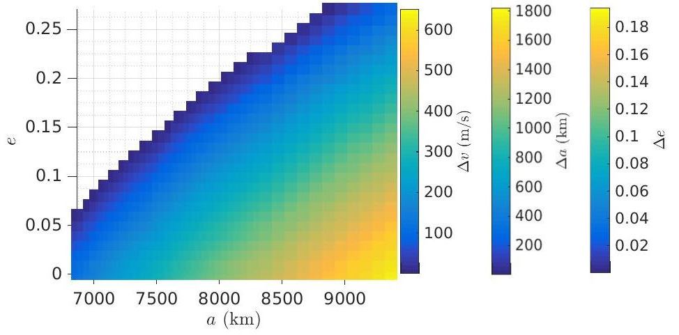
Figure 1: $\Delta v$ (m$/$s), $\Delta a$ (km) and $\Delta e$ required to reenter by lowering the perigee altitude down to 80 km, as a function of initial ($a$, $e$). The change in $a$ and $e$ have been obtained from Eqs. (1) assuming a tangential maneuver.

In the case that the maximum $\Delta v$ available on-board is of 100 m$/$s, a plausible value for the maneuver budget, the corresponding maximum variations achievable in $a$ and $e$ are shown in Fig. 2.

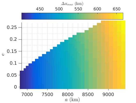
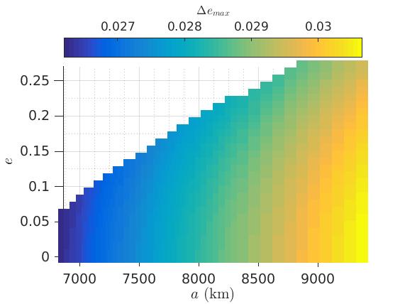
Figure 2: Maximum change in $a$ (left; in km) and $e$ (right) achievable with a $\Delta v$ of 100 m$/$s, as a function of the initial $a$ and $e$.

Concerning the maximum allowed change in inclination, the third of Eqs. (1) can be applied by assuming that the maneuver provides only a variation in $i$, leaving the other orbital elements unchanged. This is shown in Fig. 3 – left, where we display the cost of a plane change maneuver for two circular orbits at $a=R_{E}+800\,$km and $a=R_{E}+3000\,$km, respectively, in the case that the maneuver is applied at the node. Fig. 3 – right shows a close-up for $\Delta i$ up to $2^{\circ}$. The figure points out that the required $\Delta v$ to provide a change in inclination of $\Delta i=1^{\circ}$ is of the order of 100 m/s, almost independently from the initial altitude. To achieve a higher $\Delta i$, a considerable $\Delta v$ should be available: for example, the cost to allow a change in inclination by $6^{\circ}$ should be as high as 700 m$/$s for an altitude of $3000\,$km and 800 m$/$s for an altitude of $800\,$km. We also recall that the grid in inclination was set at a step of $2^{\circ}$.

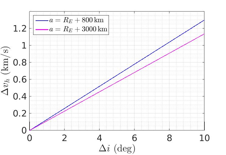
Figure 3: Cost (km/s) required to change the inclination (deg) of a circular orbit at two different altitudes: 800 km in blue, 3000 km in magenta, assuming that the maneuver is applied at the node. On the right, a close-up up to $\Delta i=2^{\circ}$.

Notice that the Gauss equations help to filter the amount of data to be examined. After this filtering, before computing the actual maneuver required to move from one orbit to the other, the implemented algorithm checks if the two orbits intersect first in projection, i.e., if the pericenter radius of the largest orbit is lower than the apocenter radius of the smallest orbit, and, if it is the case, computes the points of intersection by means of the procedure explained in [14]. At these points, the $\Delta v$ is finally computed by transforming the orbital elements into Cartesian coordinates. In this way, we take into account the change in velocity due to a possible change of all the orbital elements.

3.1 First results: low area-to-mass ratio

As an example of the single-burn strategy described above, we compute the minimum $\Delta v$ required for each initial orbit to reenter within a 50 years residual lifetime, in the case of $A/m=0.012\,$m${}^{2}/$kg. The generous 50 years limit is considered to overcome the constraint imposed by the usage of the grid, and to obtain some reentry options also for high values of semi-major axis. The results are shown in Fig. 4 – top row for 3 initial semi-major axes, $a=R_{E}+(960,\,1300,\,2100)\,$km, as a function of the initial $(i,\,e)$. Note the uniform behavior found, except for isolated points (e.g., those located around $i=40^{\circ},56^{\circ},64^{\circ},116^{\circ}$) corresponding to the dynamical resonances, described in [4]. These resonances are associated with perturbations different from the atmospheric drag, and take place in narrow regions of the $(a,e,i)$ space. For a typical value of area-to-mass ratio they can reduce the $\Delta v$ needed to reenter by an amount of the order of tens of m/s, only if exploited along with the drag.

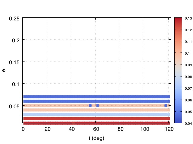
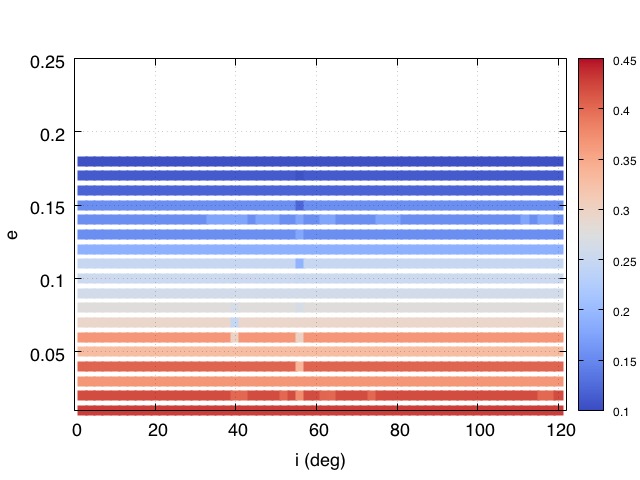
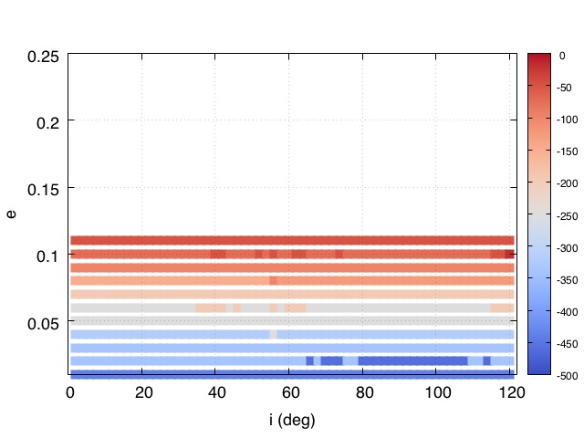
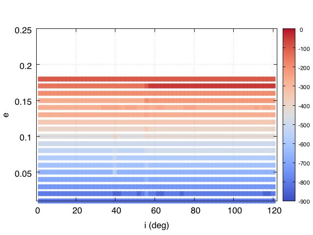
Figure 4: For $A/m=0.012\,$ m${}^{2}/$kg, as a function of initial $(i,\,e)$ in the LEO region, examples of the “minimum cost-reentry solutions” computed with a single-burn maneuver for three values of the initial semi-major axis: $a=R_{E}+960\,$km (first column), $a=R_{E}+1300\,$km (second column) and $a=R_{E}+2100\,$km (third column). The color bar shows the $\Delta v$ computed (first row, units are m/s), the corresponding $\Delta e$ (second row) and $\Delta a$ (third row, units are km).

In general, the maneuver computed with the implemented strategy aims at lowering the semi-major axis and increasing the eccentricity. When a perturbation is exploited, these changes are smaller. This is shown in Fig. 4 as well: the second row shows the $\Delta e$ associated to the minimum required $\Delta v$ for the three selected values of semi-major axis, while the third row shows the corresponding $\Delta a$. An inclination change is, instead, almost never chosen by the procedure, except for very specific cases. For this methodology, the orbital elements that can be considered as a target are the ones in the grid defined in Table 1, that is, we explore a discrete set of final conditions. In particular, the inclination step is $\Delta i=2^{\circ}$, which limits the applicability of the method, since a maneuver of $2^{\circ}$ in inclination is, in general, above the threshold of the available $\Delta v$. Considering a finer grid, i.e., $\Delta i=0.5^{\circ}$, in some cases an inclination maneuver might become more convenient than the usual semi-major axis and eccentricity one, and the exploitation of the resonant corridors would be more evident. A specific exploration of these possibilities will be discussed further in Sec. 4.

Some qualitative remarks can be done by comparing our results far from resonances with the ones shown in [15], where end-of-life deorbiting strategies for typical LEO satellites are considered. In Table 2, we recall the results shown in [15] about the highest initial orbital altitude from which it is possible to dispose a given spacecraft in compliance with the 25-year rule, accounting for either a maximum $\Delta v$ of 100 m/s or 200 m/s. Given that the orbits they considered are not exactly circular, and that no details on the area-to-mass values are provided, their results can be considered consistent with our findings. This can be inferred by looking to Fig. 4 – first row. In particular, looking to the second panel of Fig. 4, which refers to an initial orbit at $a=R_{E}+960$ km, we can see that our single-burn procedure gives a $\Delta v\simeq 130$ m/s to reenter from an initial quasi-circular orbit, while a less expensive maneuver is sufficient to deorbit from slightly more elliptical orbits. The same is true if we look to the third panel of Fig. 4, which refers to $a=R_{E}+1300\,$km; in this case, a $\Delta v\simeq 240$ m/s is required to reenter from quasi-circular orbits.

Spacecraft	$\Delta v=100$ m/s	$\Delta v=200$ m/s
Pathfinder	980 km	1370 km
Munin	910 km	1290 km
Safir-2	870 km	1240 km
Abrixas	910 km	1260 km
IRS_1C	910 km	1300 km
2420 kg-spacecraft	870 km	1250 km

Table 2: Maximum initial orbital altitude from which the given spacecraft can comply with the 25-year rule (values from [15]).

3.2 First results: high area-to-mass ratio

The results obtained in [2, 3, 4] show that in order to be compliant with the 25-year rule the exploitation of a drag sail might be successful for quasi-circular orbits up to an altitude of about 1050 km, irrespective of the initial value of inclination. On the other hand, in order to properly exploit the SRP perturbation (i.e., a solar sail) the corresponding resonant inclination bands shall be targeted. Hence, for satellites where a reasonably sized solar/drag sail can be mounted, we can conceive a deorbiting strategy of two phases: in the first one a relatively small maneuver is performed to reach a realm where, in the second phase, either the atmospheric drag or the solar radiation pressure can be exploited to reenter by means of a passive sail. For the $\Delta v-$threshold imposed in this case, namely, 100 m$/$s, a sail of $A/m=1$ m${}^{2}/$kg, can be effective up to $a=R_{E}+3000$ km, also for quasi-circular orbits, but only if the satellite is moving in the vicinity of one of the inclination corridors at $i\approx 40^{\circ}$ and $i\approx 80^{\circ}$, corresponding to the two main SRP resonances (see, e.g., [11] for details).

As in Fig. 4, in Fig. 5 – first row we show the minimum $\Delta v$ computed to reenter in 25 years exploiting a drag or a solar sail (given the maximum threshold of 100 m$/$s) in the $(i,\,e)$ space for three values of the initial semi-major axis, $a=R_{E}+(1300,\,1600,\,2900)\,$km.

Figure 5: For $A/m=1\,$ m${}^{2}/$kg, as a function of initial $(i,\,e)$ in the LEO region, examples of the “minimum cost-reentry solutions” for three values of the initial semi-major axis: $a=R_{E}+1300\,$km (first column), $a=R_{E}+1600\,$km (second column) and $a=R_{E}+2900\,$km (third column). The color bar shows the $\Delta v$ computed (first row, units are m/s), the corresponding $\Delta e$ (second row) and $\Delta a$ (third row, units are km).

In the plots, white regions denote initial conditions for which there does not exist a solution, i.e., the solutions computed are characterized by a $\Delta v$ higher than the limit set. Empty squares represent natural solutions which do not need any impulsive strategy but only the usage of a sail, while colored squares refer to initial conditions requiring both an impulsive maneuver and the exploitation of a sail. Empty and colored squares may overlap, because we considered all the possible $(\Omega,\omega)$ configurations of the grid. In Fig. 5 – second row we show the change in eccentricity corresponding to the minimum $\Delta v$ for the same three values of semi-major axis, while in the third row we present the corresponding variation in semi-major axis. For each case considered, a change in inclination was never chosen by the procedure, since it never corresponds to a minimum cost solution.

4 Single-burn strategy based on the dynamical effects

The algorithm just described allows to compute, for a given initial condition, various solutions, which can differ not only in the $\Delta v$ required to reenter, and thus in the target orbital elements, but also in the lifetime. In particular, as mentioned above, being based on the grid discretization adopted in the mapping of the LEO phase space, our results are step-wise continuous. Hence, for some specific orbits, we cannot target a specific value of the residual lifetime (hence of the required $\Delta v$), while the only information available is whether the solution is compliant with the 25-year (or “desired”-year) rule or not. Moreover, due to the steps in $(a,e,i)$ adopted in the grid, the target conditions fulfilling the 25-year rule are also step-wise continuous, and thus, we can miss important information. For instance, in the non-resonant case, it can happen that for a given value of $a$ there is a value of $e$ in the grid which corresponds to a 25-year reentry, but for the next point of $a$ in the grid the eccentricity available in the grid is associated with a lifetime slightly higher than 25 years, and thus the above methodology discards such semi-major axis as a possible target. Nevertheless, note that, once the algoritm is implemented and tested, there is the possibility to conveniently refine the grid as a future task.

In general, we can be interested in computing the optimal maneuver, exploiting a maximum available $\Delta v$ and requiring also for a maximum residual lifetime. In this case, the assumption that the target orbit belongs to the grid may become too severe. For these reasons, we have attempted to employ the numerical cartography computed in LEO in a different way. The theoretical analysis performed (see, e.g., [2, 3, 4, 11]) show that, for a given semi-major axis and eccentricity of the initial orbit, the dynamical instabilities, triggered by perturbations different from the atmospheric drag, can play a role only at specific values of inclination. In particular, the resonant dynamics is effective within narrow corridors in inclination, limited by at most 2^∘ around the resonant value of inclination. Outside these regions, the computed lifetime and the maximum eccentricity achieved during propagation do not depend significantly on the initial inclination. This information can be exploited in two ways, in order to check if a reentry can be achieved in a given time:

• if the inclination of the departure orbit does not belong to the resonant corridor and the $\Delta v-$budget does not allow to reach it, then the initial reentry state is defined only in terms of semi-major axis and eccentricity, and the transfer will be driven by the atmospheric drag;

• if a resonant value of inclination can be targeted with the available propellant on-board, then the impulsive strategy aims at changing semi-major axis, eccentricity and inclination, and the transfer will be driven by the atmospheric drag in combination with another perturbation.

For a given departure orbit, we can compute a set of displacements in terms of semi-major axis, eccentricity and inclination, say $(\delta a,\delta e,\delta i)$, defined as the difference, in terms of $(a,e,i)$, between the initial conditions of the departure orbit and all the possible target conditions associated to a reentry in the desired time. Such conditions are determined by either the effect of the atmospheric drag or the atmospheric drag together with another perturbation. On the other hand, the values $(\Delta a,\Delta e,\Delta i)$ defined in Eqs. (1) provide an upper limit to the possible displacement achievable with a given $\Delta v$. Thus, comparing the set $(\Delta a,\Delta e,\Delta i)$ with each set $(\delta a,\delta e,\delta i)$, we can find out if there exists at least one reentry solution given the departure orbit, the $\Delta v-$budget and the area-to-mass ratio.

For a given departure orbit, we can compute:

• the target values $(\delta a,\delta e)_{d}$ associated with a reentry assisted only by the drag in the desired time span;

• the target values $(\delta a,\delta e,\delta i)_{p}$ associated with a reentry assisted by the drag plus another dynamical perturbation in the desired time span.

So, we may encounter the following situations:

• $\delta a_{d}\leq\Delta a$ and $\delta e_{d}\leq\Delta e$ for one or more target conditions, that is, the reentry is feasible by changing semi-major axis and eccentricity;

• $\delta a_{p}\leq\Delta a$ and $\delta e_{p}\leq\Delta e$ and $\delta i_{p}\leq\Delta i$, for one or more target conditions, that is, the reentry is feasible by changing semi-major axis, eccentricity and inclination;

• $\delta a_{d}>\Delta a$ or $\delta e_{d}>\Delta e$, that is, we cannot reenter only exploiting the effect of the atmospheric drag;

• $\delta a_{p}>\Delta a$ or $\delta e_{p}>\Delta e$ or $\delta i_{p}>\Delta i$, that is, the reentry cannot be assisted by perturbations different from drag.

Note that, if more reentry conditions can be targeted, the selection can be made following different criteria. In particular, one can select the less expensive strategy in terms of $\Delta v$ or exhaust all the available propellant to speed-up the reentry and passivate the spacecraft.

4.1 Target conditions: non-resonant case

As mentioned above, the definition of the target conditions depends on whether the reentry is driven by the atmospheric drag alone or in combination with another perturbation. That is, it depends if we cannot exploit a resonant condition or if it becomes possible.

In the former case, investigating the maps and considering also the frequency characterization of the eccentricity evolution described in [10], we selected $i=10^{\circ}$ as a reference value of initial inclination corresponding to a “non-resonant” dynamical behavior. We selected two possible values of the residual lifetime: 25 years and the more compelling value of 10 years. Then, for each initial semi-major axis of the grid we identified the required eccentricity to reenter in 25 or 10 years. The results for both area-to-mass ratios are shown in Fig. 6, where we show, on the left, the required $e$ and, on the right, the pericenter altitude $h_{p}$ to reenter as a function of the initial $a$. These $a-e$ configurations are the target conditions for the disposal strategy.

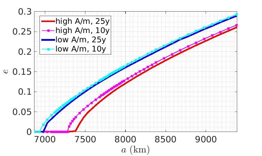
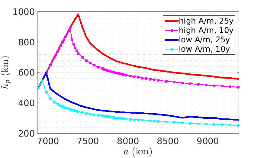
Figure 6: On the left: initial $e$ required to reenter in 25 years (solid line) or 10 years (squares) for each $a$ of the grid at initial $i=10^{\circ}$, for both $A/m=0.012$ m${}^{2}/$kg and $A/m=1$ m${}^{2}/$kg. On the right: initial pericenter altitude, $h_{p}$, required to reenter in 25 years (solid line) or 10 years (squares) for each $a$ of the grid at initial $i=10^{\circ}$, for both $A/m=0.012$ m${}^{2}/$kg and $A/m=1$ m${}^{2}/$kg.

Given our assumption on the solar flux, in the case of low $A/m$ ratio, the atmospheric drag turns out to be effective in driving a reentry from quasi-circular orbits only up to altitudes of about 600 km for a residual lifetime of 25 years and of 550 km for a lifetime of 10 years, while at higher altitudes a reentry within 25 years or less becomes feasible only if the initial orbit is gradually more eccentric. For $A/m=1$ m${}^{2}/$kg, the drag dominates the dynamics up to an altitude of about 1000 km and a reentry within 25 years can be achieved. A reentry within 10 years, instead, is feasible if the pericenter altitude is below 900 km.

4.2 Target conditions: resonant case

In the resonant case, instead, the target conditions are $a-e-i$ configurations, which correspond to a resonance involving the rate of precession of the ascending node $\dot{\Omega}$ and of the argument of pericenter $\dot{\omega}$. Solar radiation pressure, lunisolar perturbations and the 5th zonal harmonics produce a long-term variation in eccentricity, which becomes quasi-secular when a well-defined combination of $\dot{\Omega}$ and $\dot{\omega}$ tends to zero. In LEO, assuming the two values of $A/m$ adopted in this work, the rate of $\Omega$ and $\omega$ can be approximated considering only the effect of the oblateness of the Earth. As a consequence, the growth of eccentricity and the corresponding reduction in lifetime can be expressed as a function of $(a,e,i)$. Thus, given the semi-major axis and eccentricity, the resonances are arranged along inclination curves. An example of the resonant curves as a function of $i$ and $a$ fixing $e=0.01$ is shown in Fig. 7: the green curves refer to resonances due to SRP, the cyan curve to 5th degree zonal harmonic and the ocher curves to lunisolar perturbations. More details can be found in [2, 4, 11]. In order to benefit from the dynamical perturbation responsible of the resonance and to facilitate a reentry, the initial orbit must lay within one of the highlighted resonant corridors. Associated with such values of inclination, the required eccentricity to reenter within 25 years can be significantly lower than at the nearby inclinations.

Figure 7: As a function of the initial inclination (deg) and semi-major axis (km), we show the location of the resonances found to play a role in the LEO region. The color of the curves describe the nature of the resonance: green for SRP, cyan for 5th degree zonal harmonic, ocher for lunisolar perturbations. The curves have been computed for $e=0.01$.

The initial $a$ and $i$ where the resonant behavior allows for a lower target eccentricity are highlighted in Fig. 8 for the case $A/m=0.012$ m${}^{2}/$kg. The color bar refers to the relative difference $\Delta e_{target}=(e_{d}-e_{p})/e_{d}$ between the reference target eccentricity at $i=10^{\circ}$, $e_{d}$, and the target eccentricity required at a resonant inclination, $e_{p}$.

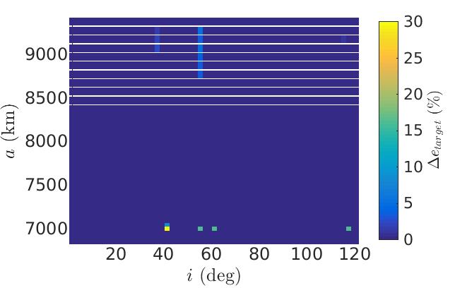
Figure 8: Relative difference $\Delta e_{target}$ (in %) between the eccentricity needed to reenter in 25 years at $i=10^{\circ}$ ($e_{d}$) and the eccentricity of the target orbit in case of a resonance which assists the reentry ($e_{p}$), for $A/m=0.012$ m${}^{2}/$kg, as a function of the initial $i$ and $a$.

As expected for the low value of area-to-mass ratio, most of the figure is dark blue, except a few specific points where resonances are effective in reducing the target eccentricity. Writing the disturbing function due to a given perturbation as a sinusoidal term of argument $\psi$ (see [11] for more details), the observed resonances correspond to (refer also to Fig. 7):

• $\dot{\psi}=\dot{\Omega}+\dot{\omega}-\dot{\lambda}_{S}\simeq 0$, around $i=40^{\circ}$ and $i=116^{\circ}$, associated to SRP (see, e.g., [16]), where $\lambda_{S}$ is the longitude of the Sun with respect to the ecliptic plane;

• $\dot{\psi}=\dot{\Omega}+2\dot{\omega}$ at $i=56^{\circ}$, which is the well-known lunisolar gravitational resonance; moreover, for altitudes above $h=2000$ km, at the same inclinations are effective also two resonances due to SRP corresponding to $\dot{\psi}=\dot{\omega}-\dot{\lambda}_{S}\simeq 0$ and $\dot{\psi}=\dot{\Omega}+\dot{\omega}+\dot{\lambda}_{S}\simeq 0$, respectively (see, e.g., [16]);

• $\dot{\psi}=\dot{\omega}\simeq 0$ at $i=63.4^{\circ}$, due to the doubly-averaged lunisolar gravitational perturbations and to the 5th-degree zonal harmonics (see, e.g., [17, 18, 19, 4]).

Note that Fig. 8 was obtained displaying the data computed by the numerical cartography, and analogous results are available for all the explored values of eccentricity. The figure allows to conclude that in practice, when a reentry within 25 years is required, the benefit due to resonances is limited in the case of low $A/m$ ratio. This fact does not disagree with the results on the global LEO dynamical mapping found by the authors and described, e.g., in [2, 3, 4]. Indeed, we observed that resonances could assist a reentry at specific inclinations, given semi-major axis and eccentricity, by lowering the residual lifetime of some tens of years, in combination with the atmospheric drag. The observed decrease in lifetime was, however, compliant with the 25-year rule only in a few cases for $A/m=0.012$ m${}^{2}/$kg.

In the case of $A/m=1$ m${}^{2}/$kg, the approach is different. The target $a-e-i$ conditions are not obtained from the numerical cartography, but they can be computed analytically. Due to the high area-to-mass ratio, the only resonances which matter are those associated with the SRP. In this case, considering only the first order terms, the disturbing function can be written as a sum of sinusoidal terms with argument:

$$\psi=\alpha\Omega\pm\omega\pm\lambda_{s}\,\,\,\,\,\,(\alpha=0,1)\,,$$

corresponding to six different resonances, indexed as in Table 3 (see, e.g., [20]). In [11] we developed a simplified analytical theory which allows to compute the supreme norm of the variation in eccentricity induced by the six first order SRP resonances. The maximum eccentricity variation that can be achieved at the resonance $j$ ($j=1,..6$) can be estimated as:

$$\Delta e_{SRP,j}=\left|\frac{3}{2}\,P\,C_{R}\,\frac{A}{m}\,\frac{\sqrt{1-e^{2}}}{na}\,\frac{T_{j}}{\psi_{j}}\right|\,,$$ (2)

where $P$ is the solar radiation pressure, $C_{R}$ the reflectivity coefficient, $n$ the mean motion of the spacecraft and the explicit expression for $T_{j}$ is shown in Table 3 (see, e.g., [11]).

$j$	$\psi_{j}$	$T_{j}$
1	$\Omega+\omega-\lambda_{S}$	$\cos^{2}(\epsilon/2)\cos^{2}(i/2)$
2	$\Omega-\omega-\lambda_{S}$	$\cos^{2}(\epsilon/2)\sin^{2}(i/2)$
3	$\omega-\lambda_{S}$	$1/2\sin(\epsilon)\sin(i)$
4	$\omega+\lambda_{S}$	$-1/2\sin(\epsilon)\sin(i)$
5	$\Omega+\omega+\lambda_{S}$	$\sin^{2}(\epsilon/2)\cos^{2}(i/2)$
6	$\Omega-\omega+\lambda_{S}$	$\sin^{2}(\epsilon/2)\sin^{2}(i/2)$

Table 3: For each first order resonance due to SRP ($j=1,..6$), we show the argument $\psi_{j}$ and the corresponding function $T_{j}$ ($\epsilon$ refers to the obliquity of the ecliptic).

The comparison between the theoretical variation in eccentricity, $\Delta e_{SRP,j}$, due to each resonance and the eccentricity increment, $\Delta e_{FOP}$, computed over 120 years of propagation with FOP, is shown in Fig. 9 as a function of the inclination, for the initial orbit: $a=R_{E}+2200\,$km, $e=0.001$, $\Omega=\omega=0^{\circ}$. In this case, the step in the inclination grid was set to $\Delta i=0.5^{\circ}$. This plot, together with analogous ones for different values of $(a,e)$, confirms a very good match between the theoretical and computed variation of eccentricity, supporting the assumption that a first-order theory describes accurately the dynamics induced by SRP.

Figure 9: Comparison between the maximum eccentricity variation, computed with Eq. (2), and the eccentricity variation provided by FOP, as a function of inclination, for the initial orbit: $a=R_{E}+2200\,$km, $e=0.001$, $\Omega=\omega=0^{\circ}$.

The above expression can be used to compute the total variation in eccentricity due to SRP:

$$\Delta e_{SRP}=\sum_{j=1}^{6}\Delta e_{SRP,j}\,.$$

First, the given $\Delta v$ provides a set $(a,e,i)$ of attainable orbits that can be targeted starting from the initial orbit. Note that the attainable set includes the initial condition itself, that is, it includes all the possible $(a,e,i)$ achievable applying a maneuver at most equal to the given $\Delta v$. Then, the reentry can be supported by SRP if the $\Delta e_{SRP}$ associated to one of the target orbits of the set ensures to reach the proper curve in Fig. 6. As an example, in Fig. 10 we show, as a function of the initial $i$ and $a$, the displacement $\Delta e_{SRP}$ induced by SRP, fixing the initial $e=0.01$. The initial orbits where SRP alone is capable of triggering the reentry can be identified comparing the computed value of $\Delta e_{SRP}$ with the eccentricity required to reenter in 25 years, corresponding to the red line in Fig. 6 – left. For example, for $A/m=1$ m${}^{2}/$kg Fig. 6 – left shows that at an altitude of 2200 km the eccentricity needs to be, at least, $e=0.18$ to reenter within 25 years; thus, as shown in Fig. 10, around the resonant inclinations the growth of eccentricity induced by SRP alone ensures reentry.

Figure 10: Increase in eccentricity due to SRP as a function of the initial $a$ and $i$, for $e=0.01$ and $A/m=1$ m${}^{2}/$kg.

4.3 Results: low area-to-mass ratio

To show the possible outputs of the described disposal strategy in the case of $A/m=0.012\,$m${}^{2}/$kg, we consider two test cases whose initial orbital elements are detailed in Table 4.

	$a$ (km)	$e$	$h_{p}$ (km)	$i$ (∘)	$\Omega$ (∘)	$\omega$ (∘)
Case 1	7100	0.02	580	40.8	90	0
Case 2	7100	0.02	580	41.8	90	0

Table 4: Initial orbits selected as a reference case for $A/m=0.012\,$m${}^{2}/$kg: semi-major axis, eccentricity, altitude of the perigee, inclination, right ascension of the ascending node, argument of perigee.

The two initial orbits differ only by 1^∘ in inclination. We recall that at this altitude the resonant inclination associated to the dominant term $\psi_{1}$ due to SRP is $i_{res}=41.8^{\circ}$. Thus, the second case refers to an orbit with initial inclination corresponding exactly to a resonant value, while the first case considers an orbit lying only $1^{\circ}$ in inclination next to a resonant corridor. We assume to have an available maximum $\Delta v$ of 80 m/s. For this altitude and eccentricity, the tangential maneuver to be applied at the apogee in order to lower the perigee down to 120 km would be of 130 m/s, thus a direct reentry is not allowed. In the first case, the minimum cost solution obtained consists in applying $\Delta v_{t}=-33.6$ m/s at the apogee which corresponds to $\Delta a=-62$ km and $\Delta e=0.009$. The perigee altitude of the target orbit is $h_{p}=455.7$ km: at this altitude the effect of atmospheric drag guarantees a reentry in 25 years.

In the second case, instead, a resonant solution due to SRP can be exploited: with a total $\Delta v=28.2$ m/s, lower than the previous case, it is possible to change the semi-major axis by $\Delta a=-22$ km, the eccentricity by $\Delta e=0.003$ and the inclination by $\Delta i=0.0035^{\circ}$, targeting a new orbit where SRP can be exploited in order to achieve a reentry in 25 years. This result confirms that we can take advantage from a resonance to facilitate a reentry, requiring a lower $\Delta v-$budget. Note, however, that the inclination range where the perturbation is effective is very narrow and that the gain in terms of the required $\Delta v$ is also limited.

A further interesting information concerns the required propellant mass to perform the computed maneuver. Following [13], the propellant mass required to perform the maneuver is given by:

$$\frac{m_{0}-m_{f}}{m_{0}}=1-\exp\left(-\frac{\Delta v}{w_{e}}\right)\,,$$ (3)

where $w_{e}$ is the exhaust velocity. In Table 5, we compare the results we have obtained with the ones shown in [13] - Chapter 6, for some representative altitudes. In columns 2–3 we show the maneuver and the propellant mass fraction, $\Delta v_{K}$ and $(\Delta m/m_{0})_{K}$, respectively, reported in [13] for a direct deorbiting from a circular orbit at altitude $H$ to an elliptical orbit with a perigee altitude $H_{p}=80$ km, assuming $w_{e}=2747$ m/s. In columns 4–5 we show the maneuver and the propellant mass fraction, respectively, arising from our analysis for an initial quasi-circular orbit ($e=10^{-3}$), considering the minimum cost deorbiting option complying with the 25-year rule and the $A/m=0.012\,$m${}^{2}/$kg ratio. The initial inclination has been set at $i=10^{\circ}$, far from any resonance. The same $w_{e}$ is applied to evaluate our outcome. From the table, it is apparent the well-known benefit of choosing a 25-year disposal reentry rather than a direct one, in terms of $\Delta v$ cost and mass consumption.

$H$ (km)	$\Delta v_{K}$ (m/s)	$(\Delta m/m_{0})_{K}$ (%)	$\Delta v$ (m/s)	$\Delta m/m_{0}$ (%)
800	199.4	7.0	75.0	2.7
900	224.3	7.8	123.0	4.4
1000	248.6	8.6	135.0	4.8
1100	272.3	9.4	162.0	5.7
1200	295.4	10.2	187.0	6.6
1300	317.9	10.9	211.5	7.4
1400	339.9	11.6	234.0	8.2
1500	361.5	12.3	256.5	8.9
1600	382.5	13.0	276.0	9.5

Table 5: Comparison between the maneuver and propellant mass fraction corresponding to a perigee-lowering strategy down to 80 km [13], and our results to reenter from a quasi-circular orbit ($e=10^{-3}$) in 25 years.

Moreover, if we recall Table 2 from [15] discussed in Sec. 3.1, we can observe that the results shown in the fourth column of Table 5 at altitudes of $800-900\,$ km and $1200-1300\,$km are qualitatively in agreement with the results shown in Table 2 for the cases of, respectively, a maximum available $\Delta v$ of 100 km/s or 200 km/s to reenter in 25 years.

Finally, we consider the results reported in [21] - Fig. 6, where the propellant mass fraction is plotted as a function of the required remaining lifetime for two circular orbits at altitudes $H=800$ km and $H=1400$ km, respectively, and two ballistic coefficients (20 and 200 kg/m², respectively, corresponding to $A/m=0.05$ m²/kg and $A/m=0.005$ m²/kg), assuming a bit lower exhaust velocity, $w_{e}=2550$ m/s ($I_{sp}=260$ s instead of $I_{sp}=280$ s). From Table 5 we find that our outcome for a reentry in 25 years gives a required mass fraction of $2.7\%$ to ensure a reentry from an initial quasi-circular orbit at $H=800$ km (which grows to $2.9\%$ if we assume the same $w_{e}$ as in [21]) and a mass fraction of $8.2\%$ for a reentry from an initial orbit at $H=1400$ km. These values are comparable or even better than the results shown in Fig. 6 of [21], supporting the advantages that can be taken from this study.

4.4 Results: high area-to-mass ratio

To show some illustrative results in the case that an area augmentation device is available on-board the spacecraft, we consider two couples of initial orbits, whose orbital elements together with the maximum $\Delta v$ available on-board are shown in Table 6.

	$a$ (km)	$e$	$h_{p}$ (km)	$i$ (∘)	$\Omega$ (∘)	$\omega$ (∘)	$\Delta v$ (m/s)
Case 1a	7900	0.001	1514	10	0	0	60
Case 1b	7900	0.001	1514	40.2	0	0	60
Case 2a	8170	0.01	1710	10	90	0	260
Case 2b	8170	0.01	1710	40	90	0	260

Table 6: Initial orbits selected as a reference case for $A/m=1\,$m${}^{2}/$kg: semi-major axis, eccentricity, altitude of the perigee, inclination, right ascension of the ascending node, argument of perigee, maximum $\Delta v$ available on-board.

The first two cases refer to a quasi-circular orbit at an altitude $h=1522$ km and differ only in inclination. At this altitude, the resonant inclination associated to $\dot{\psi}_{1}\simeq 0$ is $i_{res}=39.7^{\circ}$. Thus, the inclination of orbit 1a is very far from any resonance, while the inclination of orbit 1b is only $0.5^{\circ}$ next to the resonant value. Moreover, we assume to have a maximum $\Delta v$ of 60 m/s available on-board. The $\Delta v$ required at the apogee to lower the perigee altitude down to 120 km is 350 m/s, thus a direct reentry is not feasible. In the case of orbit 1a, the available $\Delta v$ can provide the maximum displacements $\Delta a=-133$ km and $\Delta e=0.017$, corresponding to a perigee altitude of the target orbit of $h_{p}=1250$ km, which is too high to achieve a natural reentry within 25 years. For the initial orbit 1b, SRP can, instead, be exploited. A maneuver of $\Delta v=27.6$ m/s provides the following variations in the orbital elements: $\Delta a=-60$ km, $\Delta e=0.0076$ and $\Delta i=0.04^{\circ}$. Then, at this target orbit the resonance due to SRP leads to a variation in eccentricity of $\Delta e_{SRP}=0.091$, which ensures a reentry within 25 years.

The two orbits labeled as case 2 have an altitude of $h=1792$ km and differ, again, only in inclination. The resonant inclination associated to $\dot{\psi}_{1}\simeq 0$ at this altitude is $i_{res}=38.9^{\circ}$. For this case the maximum $\Delta v$ available is significantly higher than the previous case: despite a value of 260 m/s is not realistic for most of the practical cases, we selected such a high $\Delta v$ in order to identify a test case where reentry can be achieved also without exploiting a resonance. The $\Delta v$ required at the apogee to lower the perigee altitude down to 120 km is now 390 m/s, thus a direct reentry is not possible. Nevertheless, for test case 2a it exists a solution to reenter in 25 years, which consists in a tangential maneuver $\Delta v_{t}=-230$ km/s applied at the apogee, corresponding to the variations $\Delta a=-533$ km and $\Delta e=0.0659$. In the case of initial orbit 2b, we can exploit a SRP resonance, even if the initial inclination is now $1^{\circ}$ next to the resonant inclination. First, a single-burn maneuver of $\Delta v=151$ m/s moves the spacecraft to a target orbit by means of the following variations: $\Delta a=-344$ km, $\Delta e=0.042$ and $\Delta i=0.207^{\circ}$. Then, SRP drives a growth of eccentricity up to $\Delta e_{SRP}=0.045$ and a reentry within 25 years is achieved.

5 Discussion and conclusions

In this paper, we have presented a discussion on the possible end-of-life disposal reentry strategies in LEO, exploiting one impulsive maneuver and/or the effect of dynamical perturbations. Taking advantage of the detailed LEO cartography obtained by the authors in the framework of the H2020 ReDSHIFT project, first of all we have presented a single-burn disposal strategy based on the grid adopted for the cartography and shown in Table 1. Observing that the assumption to dispose the spacecraft into a target orbit belonging to the grid can become too severe, we have then presented a different but synergic disposal strategy based on the physical explanation of the behavior revealed by the cartography. In particular, we focus on the possibility of exploiting dynamical resonances, mainly due to SRP, to facilitate a reentry. We can conclude that, as long as the initial inclination of the spacecraft is within or nearby a resonant corridor, the SRP perturbation alone can be exploited to reenter if an area augmentation device is available on-board, while in the case of low $A/m$ ratio we can take advantage from the resonant behavior only in combination with the effect of atmospheric drag. The clear benefit that can be achieved by exploiting a resonance to reenter highlights the importance of choosing a good initial condition from the very early phases of the mission. The inclination, in particular, shall be selected, trying to find a trade-off between mission objectives, operational constraints and end-of-life opportunities. Given the cost of a plane change maneuver and the narrow realm of the dynamical resonances, we recommend a value close enough to a natural highway, towards which the satellite could be moved at the end-of-life.

The analysis presented provides general important indications on how a single-burn strategy shall be applied for mitigation purposes, both in the perspective of a reentry and for a graveyard solution. As a matter of fact, far from the resonances, the eccentricity can be considered as constant, that is, the relative periodic variation is not significant with respect to the initial value. This is shown in Fig. 11, where we have represented the maximum variation of the eccentricity relative to the initial value, i.e., $(e_{max}-e_{min})/e_{in}$ computed with FOP over 120 years, for all values of initial semi-major axis such that the pericenter altitude is higher than 600 km.

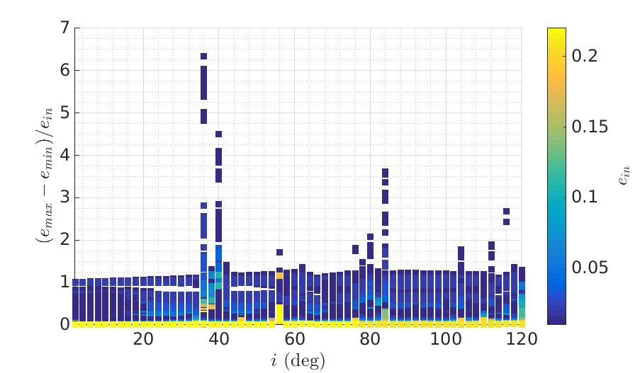
Figure 11: $(e_{max}-e_{min})/e_{in}$ for all the initial conditions such that $h_{p}>600$ km at the initial epoch 2020 and $A/m=0.012$ m²kg. The color bar shows the initial value of eccentricity.

When the eccentricity does not experience dramatic changes, i.e., outside the resonance corridors, we expect that by changing the initial epoch, the general behavior depicted, for example, in Fig. 4 will not change. This also means that if a spacecraft is left above the altitudes where the drag is effective and outside the resonance corridors, it will stay there almost forever, because its orbit can be considered stable. This information can be positively used when the required $\Delta v-$budget to reenter is too high, and thus a graveyard solution must be selected. In this case, the best option consists in the closest circular orbit above an altitude of 2000 km, outside the resonance corridors. Note also that, in this case, the maneuver should be applied considering the spatial density of the target region, or the criticality of the corresponding shells (see [22] and [23]). In particular it is worth stressing that, even if the residual propellant on-board would not allow for a proper disposal maneuver (either towards a re-entry solution or towards a super-LEO graveyard zone), the information on the criticality of the surrounding altitude shells might suggest a small maneuver to allow the positioning in a low-criticality nearby shell, thus minimizing the long-term environmental impact of the abandoned spacecraft.

Future directions include the possibility of targeting the conditions described here by means of two or more maneuvers and evaluating the collision risk experienced by specific reentry trajectories.

6 Acknowledgements

This work is funded through the European Commission Horizon 2020, Framework Programme for Research and Innovation (2014-2020), under the ReDSHIFT project (grant agreement n^∘ 687500).

We are grateful to Camilla Colombo, Ioannis Gkolias, Kleomenis Tsiganis, Despoina Skoulidou for the useful discussions on the problem.

References

- [1] A. Rossi, E. M. Alessi, G. Schettino, J. Beck, T. Schleutker, F. Letterio, J. Becedas Rodriguez, F. Dalla Vedova, H. Stokes, C. Colombo, S. Walker, S. Yang, K. Tsiganis, D. Skoulidou, A. Rosengren, E. Stoll, V. Schaus, R. Popova, A. Francesconi, and The ReDSHIFT team, the H2020 project ReDSHIFT: overview, first results and perspectives, Proceedings of the 7th European Conferences on Space Debris, Darmstadt, Germany, April 18-21, 2017.
- [2] E. M. Alessi, G. Schettino, A. Rossi, G. B. Valsecchi, LEO Mapping for Passive Dynamical Disposal, Proceedings of the 7th European Conferences on Space Debris, Darmstadt, Germany, April 18-21, 2017.
- [3] E. M. Alessi, G. Schettino, A. Rossi, G. B. Valsecchi, Dynamical Mapping of the LEO Region for Passive Disposal Design, Proceedings of the 68th International Astronautical Congress (IAC), paper IAC-17.A6.2.7, Adelaide, Australia, September 25-29, 2017.
- [4] E. M. Alessi, G. Schettino, A. Rossi, G. B. Valsecchi, Natural Highways for End-of-Life Solutions in the Region, Cel. Mec. Dyn. Astron. (2018), accepted.
- [5] A. J. Rosengren, D. K. Skoulidou, K. Tsiganis, G. Voyatzis, Dynamical cartography of Earth satellite orbits, Adv. Space Res. (2017), submitted.
- [6] IADC (Inter-Agency Space Debris Coordination Committee), IADC Space Debris Mitigation Guidelines, IADC-02-01, Revision 1 (2007).
- [7] L. Anselmo, A. Cordelli, P. Farinella, C. Pardini, A. Rossi, Study on long term evolution of Earth orbiting debris, ESA/ESOC contract n. 10034/92/D/IM(SC) (1996).
- [8] A. Rossi, L. Anselmo, C. Pardini, R. Jehn, G. B. Valsecchi, The new space debris mitigation (SDM 4.0) long term evolution code, Proceedings of the 7th European Conference of Space Debris, Paper ESA SP-672, Darmstadt, Germany, March 30-April 2, 2009.
- [9] C. Colombo, A. Rossi, F. Dalla Vedova, Drag and solar sail deorbiting: re-entry time versus cumulative collision probability, Proceedings of the 68th International Astronautical Congress, paper IAC-17.A6.2.8, Adelaide, Australia, September 25-29, 2017.
- [10] G. Schettino, E. M. Alessi, A. Rossi, G. B. Valsecchi, Characterization of Low Earth Orbit dynamics by perturbation frequency analysis, 68th Inter national Astronautical Congress, paper number IAC-17-C1.9.2. Adelaide, Australia, September 25-29, 2017.
- [11] E. M. Alessi, G. Schettino, A. Rossi, G. B. Valsecchi, Solar radiation pressure resonances in Low Earth Orbits, Mont. Not. R. Astron. Soc., 473 (2018) 2407-2414.
- [12] D. A. Vallado, Fundamentals of Astrodynamics and Applications, fourth ed., Microcosm Press, Hawthorne (CA), 2013.
- [13] H. Klinkrad, Space Debris. Models and Risk Analysis, Springer - Praxis Publishing Ltd., Chichester (UK), 2006.
- [14] G. F. Gronchi, An algebraic method to compute the critical points of the distance function between two keplerian orbits, Cel. Mec. Dyn. Astron., 93 (2005) 297-332.
- [15] R. Janovsky, M. Kassebom, H. Lubbersted, O. Romberg, H. Burkhardt, M. Sippel, G. Krulle, B. Fritsche, End-of-Life de-orbiting strategies for satellites, Proceedings of the International Astronautical Congress, paper IAC-03-IAA.5.4.05, Bremen, Germany, September 29-October 3, 2003.
- [16] S. Hughes, Satellite orbits perturbed by direct solar radiation pressure: general expansion of the disturbing function, Plan. Space Sci., 25 (1977) 809-815.
- [17] G. E. Cook, Luni-solar perturbations of the orbit of an Earth satellite, Geophys. J. Royal Astron. Soc., 6 (1962) 271-291.
- [18] S. Hughes, Earth Satellite Orbits with Resonant Lunisolar Perturbations. I. Resonances Dependent Only on Inclination, Proceedings of the Royal Society of London. Series A, Mathematical and Physical Sciences, 372 (1980) 243-264.
- [19] R. H. Merson, The Motion of a Satellite in an Axi-symmetric Gravitational Field, Geophys. Journal 4 (1961) 17-52.
- [20] A. V. Krivov, L. L. Sokolov, V. V. Dikarev, Dynamics of Mars-Orbiting Dust: Effects of Light Pressure and Planetary Oblateness, Cel. Mech. Dyn. Astron. 63 (1995) 313-339.
- [21] R. Walker, C. E. Martin, Cost-effective and robust mitigation of space debris in Low Earth Orbit, Adv. Space Res., 34 (2004) 1233–1240.
- [22] A. Rossi, G. B. Valsecchi, E. M. Alessi, The criticality of spacecraft index, Adv. Space Res., 56 (2015) 449–460.
- [23] C. Bombardelli, E. M. Alessi, A. Rossi, G. B. Valsecchi, Environmental effect of space debris repositioning, Adv. Space Res., 60 (2017) 28–37.