New a priori analysis of first-order system least-squares finite element methods for parabolic problems

Abstract.

We provide new insights into the a priori theory for a time-stepping scheme based on least-squares finite element methods for parabolic first-order systems. The elliptic part of the problem is of general reaction-convection-diffusion type. The new ingredient in the analysis is an elliptic projection operator defined via a non-symmetric bilinear form, although the main bilinear form corresponding to the least-squares functional is symmetric. This new operator allows to prove optimal error estimates in the natural norm associated to the problem and, under additional regularity assumptions, in the $L^{2}$ norm. Numerical experiments are presented which confirm our theoretical findings.

1. Introduction

In this work we analyse a time-stepping scheme based on least-squares finite element methods for a first-order reformulation of the evolution problem

(1a) $$\dot{u}-{\rm div\,}\boldsymbol{A}\nabla u-\boldsymbol{\beta}\cdot\nabla u+\gamma u =f \text{in }(0,T)\times\Omega,$$

(1b) $$u =0 \text{in }(0,T)\times\partial\Omega,$$

(1c) $$u(0,\cdot) =u^{0} \text{in }\Omega.$$

The coefficients $\boldsymbol{A}\in L^{\infty}(\Omega)_{\mathrm{sym}}^{d\times d}$, $\boldsymbol{\beta}\in L^{\infty}(\Omega)^{d}$, $\gamma\in L^{\infty}(\Omega)$ are assumed to satisfy

(2) $$L^{\infty}(\Omega)\ni\tfrac{1}{2}{\rm div\,}\boldsymbol{\beta}+\gamma\geq 0,\quad\text{and}\quad\lambda_{\mathrm{min}}(\boldsymbol{A})\geq\alpha_{0}>0\quad\text{a.e. in }\Omega.$$

This ensures that Eq. 1 admits a unique solution. (Here, $\lambda_{\mathrm{min}}$ denotes the minimal eigenvalue.) We refer to [4] for the analytical treatment and to [11] for an overview and analysis of different Galerkin methods. For a simpler presentation we suppose that the coefficients are independent of $t$, however, we stress that our analysis also applies in the case of time-dependent coefficients, if Eq. 2 holds uniformly in time.

Discretizations by finite elements in space and finite differences in time (also called time-stepping) are attractive for the numerical approximation of solutions of evolutions equations such as Eq. 1. This is due to the fact that such discretizations are much simpler to implement then discretizations of the space-time domain. In the context of least-squares finite element methods such time-stepping schemes have been analysed in, e.g., [9, 14, 13]. The analysis in these works include the Euler and Crank-Nicolson scheme in time. Another time-stepping approach is considered in [6, 7]. We refer also to [1, Chapter 9] for an overview on the whole topic. In accordance with the last reference, cf. [1, Section 2.2], the first step to obtain a practical least-squares discretization is to work with a first-order reformulation of the PDE at hand. This way, high regularity conditions on the discrete space are avoided, and condition numbers of underlying systems are kept at a reasonable level. If the first-order reformulation of Eq. 1 allows for the so-called splitting property, optimal a priori error estimates are known, cf. [9, 1]. It can be easily shown [9] that the method then reduces to a time-stepping Galerkin method in the primal variable, and optimal a priori error estimates can be extracted from the classical reference [11, Chapter 1]. We refer to subsection 2.3 for more details. This splitting property is quite specific and in general only holds if $\boldsymbol{\beta}=0=\gamma$ in Eq. 1. Available a priori analysis of least-squares finite element time stepping schemes does not extend to the general case $(\boldsymbol{\beta},\gamma)\neq(0,0)$. In fact, if $(\boldsymbol{\beta},\gamma)\neq(0,0)$, current literature provides optimal a priori error estimates under severe and impractical restrictions, e.g., the use of different meshes for approximations of the variables of the first-order system.

The purpose of the work at hand is to provide optimal error estimates in the $L^{2}$ norm for the scalar variable and in the natural norm associated with the problem, in particular in the case $(\boldsymbol{\beta},\gamma)\neq(0,0)$. Since the pioneering work of Mary Wheeler [12], one of the main tools in the a priori analysis of time-stepping Galerkin schemes is the elliptic projection operator, defined as the discrete solution operator on the spatial part of the parabolic PDE. The main tool in the following analysis is a new elliptic projection operator, which is defined with respect to only part of the spatial terms of the overall bilinear form. In particular, these terms constitute a non-symmetric bilinear form. At first glance this seems to be somehow counter-intuitive, since the overall bilinear form associated to the least-squares method is symmetric. Nevertheless, it turns out that this is the right choice, and it allows us to mimic some of the main ideas of well-known proofs for Galerkin finite element methods. Moreover, for the proof of optimal $L^{2}$ error estimates we show, under some regularity assumptions, that the $L^{2}$ error between a sufficient regular function and its elliptic projection is of higher order. This is done by considering solutions corresponding to problems that involve the aforementioned non-symmetric bilinear form and by using duality arguments. We stress that everything has to be analized carefully due to the fact that the bilinear form depends on the (arbitrarily small) temporal step-size.

To keep presentation simple, we consider a backward Euler scheme for time discretization. We stress that we have no reason to believe that our results do not extend correspondingly to a higher-order discretization in time (e.g., Crank-Nicolson). Likewise, the main ideas of our analysis are independent of the particular choice of (spatial) finite element spaces. However, to obtain convergence orders in terms of powers of the mesh-width $h$ we stick to standard conforming finite element spaces (piecewise polynomials for the scalar variable and Raviart-Thomas elements for the vector-valued variable) on the same simplical mesh.

1.1. Outline

The remainder of this work is given as follows: In section 2, we introduce our model problem and discrete method and discuss necessary definitions and results needed throughout our work. In particular, in subsection 2.6, we introduce and analyse the elliptic projection operator. The section 3 contains the main results (stability of the discrete method and optimal convergence rates in $L^{2}$ and energy norm) and their proofs. In section 4 we show how to extend our ideas to a different problem. Finally, in section 5 we present numerical examples.

2. Least-squares methods

2.1. Notation

Let $\Omega\subset\mathbb{R}^{d}$ denote a bounded Lipschitz domain with polygonal boundary $\Gamma:=\partial\Omega$. Let $\boldsymbol{L}^{2}(\Omega):=L^{2}(\Omega)^{d}$. We use the usual notation for Sobolev spaces $H_{0}^{1}(\Omega)$, $H^{s}(\Omega)$, ${\boldsymbol{H}}^{s}(\Omega):=H^{s}(\Omega)^{d}$, $\boldsymbol{H}({\rm div\,};\Omega):=\big{\{}{\boldsymbol{\sigma}}\in\boldsymbol{L}^{2}(\Omega)\,:\,{\rm div\,}{\boldsymbol{\sigma}}\in L^{2}(\Omega)\big{\}}$. Recall that $\|u\|\leq C_{\mathrm{F}}\|\nabla u\|$ for all $u\in H_{0}^{1}(\Omega)$, where $\|\cdot\|$ denotes the $L^{2}(\Omega)$ norm. Moreover, the $L^{2}(\Omega)$ scalar product is denoted by $(\cdot\hskip 1.42262pt,\cdot)$.

We work with the space

$$U:=H_{0}^{1}(\Omega)\times\boldsymbol{H}({\rm div\,};\Omega)$$

equipped with the ${k}$-dependent norm

$$\|(u,{\boldsymbol{\sigma}})\|_{{k}}^{2}:=\|\nabla u\|^{2}+\|{\boldsymbol{\sigma}}\|^{2}+{k}\|{\rm div\,}{\boldsymbol{\sigma}}\|^{2}.$$

The parameter ${k}>0$ corresponds to the time step later on.

Let $0=:t_{0}<t_{1}<\dots<t_{N}:=T$ denote an arbitrary partition of the time interval $[0,T]$. We call ${k}_{n}:=t_{n}-t_{n-1}$ a time step. For a simpler notation, we use upper indices to indicate time evaluations, i.e., for a time-dependent function $v=v(t;\cdot)$ we use the notation $v^{n}(\cdot):=v(t_{n};\cdot)$. Moreover, we use similar notations for discrete quantities which however are not defined for all $t\in[0,T]$. For instance, later on $u_{h}^{n}$ will denote an approximation of $u^{n}=u(t_{n};\cdot)$ where $u$ is the exact solution of Eq. 1.

Operators involving derivatives with respect to the spatial variables are denoted by $\nabla$ and ${\rm div\,}$, whereas the first and second derivate with respect to the time variable are denoted by $\dot{(\cdot)}$, $\ddot{(\cdot)}$. For vector-valued functions the time derivative is understood componentwise.

We write $A\lesssim B$ if there exists $C>0$ such that $A\leq CB$ and $C$ is independent of the quantities of interest. Analogously we define $A\gtrsim B$. If both $A\lesssim B$ and $B\lesssim A$ hold, then we write $A\simeq B$. In this work we use these notations if the involved constants only depend on the coefficients $\boldsymbol{A},\boldsymbol{\beta},\gamma$, the final time $T$, $\Omega$, some fixed polynomial degree $p\in\mathbb{N}_{0}$ of the discrete spaces, and shape-regularity of the underlying triangulation.

2.2. First-order system and least-squares method

Let $u$ denote the exact solution of Eq. 1. Introducing ${\boldsymbol{\sigma}}:=\boldsymbol{A}\nabla u$, we rewrite Eq. 1 as the equivalent first-order system

(3a) $$\dot{u}-{\rm div\,}{\boldsymbol{\sigma}}-\boldsymbol{\beta}\cdot\nabla u+\gamma u =f \text{in }(0,T)\times\Omega,$$

(3b) $${\boldsymbol{\sigma}}-\boldsymbol{A}\nabla u =0 \text{in }(0,T)\times\Omega,$$

(3c) $$u =0 \text{on }(0,T)\times\Gamma,$$

(3d) $$u(0,\cdot) =u^{0} \text{in }\Omega.$$

We approximate $\dot{u}^{n}$ by a backward difference, i.e., $\dot{u}^{n}\approx(u^{n}-u^{n-1})/{k}_{n}$. This approach naturally leads to a time-stepping method: given an approximation $\widetilde{u}^{n-1}$ of $u^{n-1}$, we consider the problem of finding $(u,{\boldsymbol{\sigma}})\in U=H_{0}^{1}(\Omega)\times\boldsymbol{H}({\rm div\,};\Omega)$ such that

(4a) $$\frac{u-\widetilde{u}^{n-1}}{{k}_{n}}-{\rm div\,}{\boldsymbol{\sigma}}-\boldsymbol{\beta}\cdot\nabla u+\gamma u =f^{n},$$

(4b) $${\boldsymbol{\sigma}}-\boldsymbol{A}\nabla u =0$$

for $n=1,\dots,N$. The last equations will be put into a variational scheme using a least-squares approach. For given data $g,w\in L^{2}(\Omega)$ we consider the functional

(5) $$J_{n}(\boldsymbol{u};g,w):={k}_{n}\|\frac{u-w}{{k}_{n}}-{\rm div\,}{\boldsymbol{\sigma}}-\boldsymbol{\beta}\cdot\nabla u+\gamma u-g\|^{2}+\|\boldsymbol{A}^{1/2}\nabla u-\boldsymbol{A}^{-1/2}{\boldsymbol{\sigma}}\|^{2}.$$

for $\boldsymbol{u}=(u,{\boldsymbol{\sigma}})\in U$. Note that Eq. 4 is an elliptic equation since ${k}_{n}>0$ and therefore admits a unique solution that can also be characterized as the unique minimizer of the problem

(6) $$\min_{\boldsymbol{v}\in U}J_{n}(\boldsymbol{v};f^{n},\widetilde{u}^{n-1}).$$

It is well-known [3] that the functional satisfies the norm equivalence

$$\|\nabla u\|^{2}+\|{\boldsymbol{\sigma}}\|^{2}+\|{\rm div\,}{\boldsymbol{\sigma}}\|^{2}\simeq J_{n}(\boldsymbol{u};0,0)$$

for all $\boldsymbol{u}=(u,{\boldsymbol{\sigma}})\in U$. In particular, standard textbook knowledge of the least-squares methodology, see [1], shows that there exists a unique minimizer if the space $U$ in Eq. 6 is replaced by some closed subspace. Note that the norm equivalence constants depend on the time step ${k}_{n}$ in general.

We introduce the bilinear forms $b_{n},a_{n}:U\times U\to\mathbb{R}$,

$$b_{n}(\boldsymbol{u},\boldsymbol{v}) :=(u\hskip 1.42262pt,-{\rm div\,}{\boldsymbol{\tau}}-\boldsymbol{\beta}\cdot\nabla v+\gamma v)+(-{\rm div\,}{\boldsymbol{\sigma}}-\boldsymbol{\beta}\cdot\nabla u+\gamma u\hskip 1.42262pt,v)$$

$$\qquad+{k}_{n}(-{\rm div\,}{\boldsymbol{\sigma}}-\boldsymbol{\beta}\cdot\nabla u+\gamma u\hskip 1.42262pt,-{\rm div\,}{\boldsymbol{\tau}}-\boldsymbol{\beta}\cdot\nabla v+\gamma v)$$

$$\qquad+(\boldsymbol{A}^{1/2}\nabla u-\boldsymbol{A}^{-1/2}{\boldsymbol{\sigma}}\hskip 1.42262pt,\boldsymbol{A}^{1/2}\nabla v-\boldsymbol{A}^{-1/2}{\boldsymbol{\tau}}),$$

$$a_{n}(\boldsymbol{u},\boldsymbol{v}) :=\frac{1}{{k}_{n}}(u\hskip 1.42262pt,v)+b_{n}(\boldsymbol{u},\boldsymbol{v})$$

for all $\boldsymbol{u}=(u,{\boldsymbol{\sigma}}),\boldsymbol{v}=(v,{\boldsymbol{\tau}})\in U$. Moreover, define for some given $w\in L^{2}(\Omega)$, the functional $F_{n}:U\to\mathbb{R}$ by

$$F_{n}(\boldsymbol{v};f^{n},w):={k}_{n}(f^{n}+\frac{w}{{k}_{n}}\hskip 1.42262pt,\frac{v}{{k}_{n}}-{\rm div\,}{\boldsymbol{\tau}}-\boldsymbol{\beta}\cdot\nabla v+\gamma v)$$

for $\boldsymbol{v}=(v,{\boldsymbol{\tau}})\in U$.

The backward Euler scheme reads as follows: For all $n=1,\dots,N$ let $U_{h}^{n}\subseteq U$ denote a closed subspace. Let $u_{h}^{0}\in L^{2}(\Omega)$ be some approximation of the initial data, i.e., $u_{h}^{0}\approx u^{0}$. For $n=1,\dots,N$ we seek solutions $\boldsymbol{u}_{h}^{n}=(u_{h}^{n},{\boldsymbol{\sigma}}_{h}^{n})\in U_{h}^{n}$ of

(7) $$a_{n}(\boldsymbol{u}_{h}^{n},\boldsymbol{v}_{h})=F_{n}(\boldsymbol{v}_{h};f^{n},u_{h}^{n-1})\quad\text{for all }\boldsymbol{v}_{h}=(v_{h},{\boldsymbol{\tau}}_{h})\in U_{h}^{n}.$$

From our discussion above we conclude:

Theorem 1.

For all $n=1,\dots,N$ Problem Eq. 7 admits a unique solution $\boldsymbol{u}_{h}^{n}\in U_{h}^{n}$. ∎

2.3. Problem decoupling for convection-reaction free problems

In the case of convection and reaction free problems, i.e., $(\boldsymbol{\beta},\gamma)=(0,0)$, one can show, see [1, 9], that the backward Euler least-squares method reduces to a simplified problem: Suppose $(\boldsymbol{\beta},\gamma)=(0,0)$ and that $\boldsymbol{A}$ is the identity. The bilinear form then reads

$$a_{n}(\boldsymbol{u},\boldsymbol{v}) =\frac{1}{{k}_{n}}(u\hskip 1.42262pt,v)+(u\hskip 1.42262pt,-{\rm div\,}{\boldsymbol{\tau}})+(-{\rm div\,}{\boldsymbol{\sigma}}\hskip 1.42262pt,v)+{k}_{n}(-{\rm div\,}{\boldsymbol{\sigma}}\hskip 1.42262pt,-{\rm div\,}{\boldsymbol{\tau}})+(\nabla u-{\boldsymbol{\sigma}}\hskip 1.42262pt,\nabla v-{\boldsymbol{\tau}})$$

$$=\frac{1}{{k}_{n}}(u\hskip 1.42262pt,v)+(\nabla u\hskip 1.42262pt,{\boldsymbol{\tau}})+({\boldsymbol{\sigma}}\hskip 1.42262pt,\nabla v)+{k}_{n}({\rm div\,}{\boldsymbol{\sigma}}\hskip 1.42262pt,{\rm div\,}{\boldsymbol{\tau}})+(\nabla u-{\boldsymbol{\sigma}}\hskip 1.42262pt,\nabla v-{\boldsymbol{\tau}})$$

$$=\frac{1}{{k}_{n}}(u\hskip 1.42262pt,v)+{k}_{n}({\rm div\,}{\boldsymbol{\sigma}}\hskip 1.42262pt,{\rm div\,}{\boldsymbol{\tau}})+(\nabla u\hskip 1.42262pt,\nabla v)+({\boldsymbol{\sigma}}\hskip 1.42262pt,{\boldsymbol{\tau}}),$$

where we have only used integration by parts. Testing with $\boldsymbol{v}_{h}=(v_{h},0)$ in Eq. 7 leads to the variational problem

$$\frac{1}{{k}_{n}}(u_{h}^{n}\hskip 1.42262pt,v_{h})+(\nabla u_{h}^{n}\hskip 1.42262pt,\nabla v_{h}^{n})=\frac{1}{{k}_{n}}(u_{h}^{n-1}\hskip 1.42262pt,v_{h})+(f^{n}\hskip 1.42262pt,v_{h}),$$

which is independent of ${\boldsymbol{\sigma}}_{h}^{j}$ for all $j=1,\dots,n$. Hence, this is the backward Euler method for the standard Galerkin scheme, where optimal error estimates are known [11]. Therefore, the least-squares problem simplifies to a well-known method. However, the situation is completely different when $(\boldsymbol{\beta},\gamma)\neq(0,0)$ because the problem does not decouple anymore and therefore does not reduce to a simplified method. We stress that our analysis below is in particular also valid for $(\boldsymbol{\beta},\gamma)\neq(0,0)$.

2.4. Discrete spaces and approximation properties

The main ideas of our analysis are independent of specific discrete spaces. However, for the analysis of convergence orders we will fix the following discrete setting. By $\mathcal{T}$ we denote a simplicial mesh on $\Omega$. As usual, $h$ denotes the biggest element diameter in $\mathcal{T}$. We will only consider uniform sequences of meshes, and we assume that our meshes are shape-regular. The discrete spaces which we will use are the space $\mathcal{S}_{0}^{p+1}(\mathcal{T})$ of globally continuous, $\mathcal{T}$-piecewise polynomials of degree at most $p+1$ satisfying homogeneous boundary conditions, and the Raviart-Thomas space $\mathcal{RT}^{p}(\mathcal{T})$ of order $p$. We will also need the space $\mathcal{P}^{p}(\mathcal{T})$ of piecewise polynomials of degree at most $p$. For the remainder of this work we consider the following discrete subspace of $U$,

$$U_{h}:=U_{h,p}:=\mathcal{S}_{0}^{p+1}(\mathcal{T})\times\mathcal{RT}^{p}(\mathcal{T}),$$

We will need certain interpolation operators mapping into the spaces. By $I^{\rm SZ}_{h,p}:H^{1}_{0}(\Omega)\rightarrow\mathcal{S}^{p+1}_{0}(\mathcal{T})$ we denote the Scott-Zhang interpolation operator from [10], by $I^{\rm RT}_{h,p}:\boldsymbol{H}({\rm div\,};\Omega)\cap{\boldsymbol{H}}^{1}(\Omega)\rightarrow\mathcal{RT}^{p}(\mathcal{T})$ the Raviart-Thomas interpolation operator [8], and by $\Pi_{h,p}:L^{2}(\Omega)\rightarrow\mathcal{P}^{p}(\mathcal{T})$ the $L^{2}(\Omega)$-orthogonal projection. We keep in mind that there the commutativity property ${\rm div\,}I^{\rm RT}_{h,p}{\boldsymbol{\sigma}}=\Pi_{h,p}{\rm div\,}{\boldsymbol{\sigma}}$.

The mesh $\mathcal{T}$ is called shape-regular if

$$\max_{T\in\mathcal{T}}\frac{\mathrm{diam}(T)^{d}}{|T|}\leq\kappa<\infty,$$

where $|T|$ denotes the volume of an element.

We make use of the spaces

$$C^{1}(\mathcal{T}) :=\big{\{}v\in L^{\infty}(\Omega)\,:\,v|_{T}\in C^{1}(\overline{T})\text{ for all }T\in\mathcal{T}\big{\}},$$

$$H^{p+1}(\mathcal{T}) :=\big{\{}v\in L^{2}(\Omega)\,:\,v|_{T}\in H^{p+1}(T)\text{ for all }T\in\mathcal{T}\big{\}},$$

where $H^{p+1}(T)$ denotes the Sobolev space on $T$. Moreover, let $\nabla_{\mathcal{T}}:H^{1}(\mathcal{T})\to L^{2}(\Omega)$ denote the elementwise gradient operator.

The following result is a simple consequence of the approximation properties of the interpolation operators mentioned above, respectively the commutativity property.

Proposition 2.

Let $\boldsymbol{u}=(u,{\boldsymbol{\sigma}})\in U$, $p\in\mathbb{N}_{0}$. Suppose that $u\in H^{p+2}(\Omega)\cap H_{0}^{1}(\Omega)$, ${\boldsymbol{\sigma}}\in{\boldsymbol{H}}^{p+1}(\Omega)$, and ${\rm div\,}{\boldsymbol{\sigma}}\in H^{p+1}(\mathcal{T})$. Then,

$$\min_{\boldsymbol{v}_{h}\in U_{h}}\|\boldsymbol{u}-\boldsymbol{v}_{h}\|_{{k}}\leq C_{\mathrm{app}}h^{p+1}(\|u\|_{H^{p+2}(\Omega)}+\|{\boldsymbol{\sigma}}\|_{{\boldsymbol{H}}^{p+1}(\Omega)}+{k}^{1/2}\|{\rm div\,}{\boldsymbol{\sigma}}\|_{H^{p+1}(\mathcal{T})})$$

The constant $C_{\mathrm{app}}>0$ only depends on shape-regularity of $\mathcal{T}$ and $p\in\mathbb{N}_{0}$. ∎

2.5. Regularity of solutions

For some given $g\in L^{2}(\Omega)$ we consider the second order elliptic problem

$$\begin{split}-{\rm div\,}\boldsymbol{A}\nabla v-\boldsymbol{\beta}\cdot\nabla v+\gamma v&=g,\\ v|_{\Gamma}&=0\end{split}$$

and the equivalent first-order problem

$$-{\rm div\,}{\boldsymbol{\tau}}-\boldsymbol{\beta}\cdot\nabla v+\gamma v =g,$$

$$\boldsymbol{A}\nabla v-{\boldsymbol{\tau}} =0,$$

$$v|_{\Gamma} =0.$$

Moreover, we consider the (dual or adjoint) problem

$$-{\rm div\,}(\boldsymbol{A}\nabla w-\boldsymbol{\beta}w)+\gamma w =g,$$

$$w|_{\Gamma} =0.$$

Throughout, we assume that $\boldsymbol{\beta}$ and $\gamma$ satisfy

(9a) $$\boldsymbol{\beta}\in C^{1}(\mathcal{T})^{d}\cap\boldsymbol{H}({\rm div\,};\Omega),\quad\gamma\in C^{1}(\mathcal{T}).$$

For the results concerning optimal rates of the $$L^{2} \Omega$$ error we additionally assume that and the coefficients are such that (for the solutions above)

(9b) $$\|v\|_{H^{2}(\Omega)}+\|{\boldsymbol{\tau}}\|_{{\boldsymbol{H}}^{1}(\Omega)}+\|w\|_{H^{2}(\Omega)}\lesssim\|g\|.$$

Remark 3.

Estimate Eq. 9b is satisfied for $d=2$ if $\Omega$ is convex, $\boldsymbol{A}$ the identity, and $\boldsymbol{\beta},\gamma$ satisfy Eq. 9a, see [5] for details on the regularity of solutions on polygonal domains.

2.6. Elliptic projection and duality arguments

In this section we introduce and analyse the so-called elliptic projection operator $\mathcal{E}_{h}:U\to U_{h}$, which will be used in the remainder of this work. As discussed in the introduction, the elliptic part of the problem is described by a non-symmetric bilinear form given by

$$\widetilde{b}_{n}(\boldsymbol{u},\boldsymbol{v}) :=(-{\rm div\,}{\boldsymbol{\sigma}}-\boldsymbol{\beta}\cdot\nabla u+\gamma u\hskip 1.42262pt,v)$$

$$\qquad+{k}_{n}(-{\rm div\,}{\boldsymbol{\sigma}}-\boldsymbol{\beta}\cdot\nabla u+\gamma u\hskip 1.42262pt,-{\rm div\,}{\boldsymbol{\tau}}-\boldsymbol{\beta}\cdot\nabla v+\gamma v)$$

$$\qquad+(\boldsymbol{A}^{1/2}\nabla u-\boldsymbol{A}^{-1/2}{\boldsymbol{\sigma}}\hskip 1.42262pt,\boldsymbol{A}^{1/2}\nabla v-\boldsymbol{A}^{-1/2}{\boldsymbol{\tau}})$$

for all $\boldsymbol{u},\boldsymbol{v}\in U$.

We analyse basic properties of $b$ and $\widetilde{b}$. For the remainder of this section we set ${k}:={k}_{n}$ and skip the index $n$ in the bilinear forms.

Lemma 4.

There exist constants $c_{b},C_{b}>0$ independent of ${k}\in(0,T]$ such that

(10) $$c_{b}\|\boldsymbol{u}\|_{{k}}^{2} \leq\min\{b(\boldsymbol{u},\boldsymbol{u}),\widetilde{b}(\boldsymbol{u},\boldsymbol{u})\},$$

(11) $$\max\{|b(\boldsymbol{u},\boldsymbol{v})|,|\widetilde{b}(\boldsymbol{u},\boldsymbol{v})|\} \leq C_{b}\|\boldsymbol{u}\|_{{k}}\|\boldsymbol{v}\|_{{k}}$$

for all $\boldsymbol{u},\boldsymbol{v}\in U$.

Proof.

We start to proof boundedness Eq. 11 of $\widetilde{b}$. The Cauchy-Schwarz inequality, the triangle inequality and Friedrich’s inequality show that

$${k}|(-{\rm div\,}{\boldsymbol{\sigma}}-\boldsymbol{\beta}\cdot\nabla u+\gamma u\hskip 1.42262pt,-{\rm div\,}{\boldsymbol{\tau}}-\boldsymbol{\beta}\cdot\nabla v+\gamma v)|$$

$$\qquad\leq{k}^{1/2}\|-{\rm div\,}{\boldsymbol{\sigma}}-\boldsymbol{\beta}\cdot\nabla u+\gamma u\|{k}^{1/2}\|-{\rm div\,}{\boldsymbol{\tau}}-\boldsymbol{\beta}\cdot\nabla v+\gamma v\|$$

$$\qquad\lesssim({k}^{1/2}\|{\rm div\,}{\boldsymbol{\sigma}}\|+\|\nabla u\|+\|u\|)({k}^{1/2}\|{\rm div\,}{\boldsymbol{\tau}}\|+\|\nabla v\|+\|v\|)\lesssim\|\boldsymbol{u}\|_{{k}}\|\boldsymbol{v}\|_{{k}}.$$

Moreover,

$$|(\boldsymbol{A}^{1/2}\nabla u-\boldsymbol{A}^{-1/2}{\boldsymbol{\sigma}}\hskip 1.42262pt,\boldsymbol{A}^{1/2}\nabla v-\boldsymbol{A}^{-1/2}{\boldsymbol{\tau}})| \lesssim(\|\nabla u\|+\|{\boldsymbol{\sigma}}\|)(\|\nabla v\|+\|{\boldsymbol{\tau}}\|)\lesssim\|\boldsymbol{u}\|_{{k}}\|\boldsymbol{v}\|_{{k}}.$$

Integration by parts yields

$$|(-{\rm div\,}{\boldsymbol{\sigma}}-\boldsymbol{\beta}\cdot\nabla u+\gamma u\hskip 1.42262pt,v)| =|({\boldsymbol{\sigma}}\hskip 1.42262pt,\nabla v)-(\boldsymbol{\beta}\cdot\nabla u\hskip 1.42262pt,v)+(\gamma u\hskip 1.42262pt,v)|\lesssim\|\boldsymbol{u}\|_{{k}}\|\boldsymbol{v}\|_{{k}}.$$

Putting altogether shows boundedness of $\widetilde{b}$. The same arguments prove boundedness of $b$ and therefore Eq. 11. It remains to show Eq. 10. First, from Eq. 2 it follows with integration by parts that

$$(u\hskip 1.42262pt,-\boldsymbol{\beta}\cdot\nabla u+\gamma u)=(u\hskip 1.42262pt,(\tfrac{1}{2}{\rm div\,}\boldsymbol{\beta}+\gamma)u)\geq 0.$$

This implies that

$$(u\hskip 1.42262pt,-{\rm div\,}{\boldsymbol{\sigma}}-\boldsymbol{\beta}\cdot\nabla u+\gamma u)=(\nabla u\hskip 1.42262pt,{\boldsymbol{\sigma}})+(u\hskip 1.42262pt,-\boldsymbol{\beta}\cdot\nabla u+\gamma u)\geq(\nabla u\hskip 1.42262pt,{\boldsymbol{\sigma}}).$$

Therefore,

$$2(u\hskip 1.42262pt,-{\rm div\,}{\boldsymbol{\sigma}}-\boldsymbol{\beta}\cdot\nabla u+\gamma u)+\|\boldsymbol{A}^{1/2}\nabla u-\boldsymbol{A}^{-1/2}{\boldsymbol{\sigma}}\|^{2}$$

$$\qquad\geq 2(\nabla u\hskip 1.42262pt,{\boldsymbol{\sigma}})+\|\boldsymbol{A}^{1/2}\nabla u\|^{2}+\|\boldsymbol{A}^{-1/2}{\boldsymbol{\sigma}}\|^{2}-2(\nabla u\hskip 1.42262pt,{\boldsymbol{\sigma}})=\|\boldsymbol{A}^{1/2}\nabla u\|^{2}+\|\boldsymbol{A}^{-1/2}{\boldsymbol{\sigma}}\|^{2}.$$

Together this yields

$$\|\boldsymbol{u}\|_{{k}}^{2} =\|\nabla u\|^{2}+\|{\boldsymbol{\sigma}}\|^{2}+{k}\|{\rm div\,}{\boldsymbol{\sigma}}\|^{2}\lesssim\|\nabla u\|^{2}+\|{\boldsymbol{\sigma}}\|^{2}+{k}\|-{\rm div\,}{\boldsymbol{\sigma}}-\boldsymbol{\beta}\cdot\nabla u+\gamma u\|^{2}$$

$$\lesssim\|\boldsymbol{A}^{1/2}\nabla u\|^{2}+\|\boldsymbol{A}^{-1/2}{\boldsymbol{\sigma}}\|^{2}+{k}\|-{\rm div\,}{\boldsymbol{\sigma}}-\boldsymbol{\beta}\cdot\nabla u+\gamma u\|^{2}$$

$$\leq 2(u\hskip 1.42262pt,-{\rm div\,}{\boldsymbol{\sigma}}-\boldsymbol{\beta}\cdot\nabla u+\gamma u)+\|\boldsymbol{A}^{1/2}\nabla u-\boldsymbol{A}^{-1/2}{\boldsymbol{\sigma}}\|^{2}+{k}\|-{\rm div\,}{\boldsymbol{\sigma}}-\boldsymbol{\beta}\cdot\nabla u+\gamma u\|^{2}=b(\boldsymbol{u},\boldsymbol{u}).$$

Coercivity of $\widetilde{b}$ follows from that of $b$, since

$$\widetilde{b}(\boldsymbol{u},\boldsymbol{u})\geq\tfrac{1}{2}b(\boldsymbol{u},\boldsymbol{u}).$$

This finishes the proof. ∎

For given $\boldsymbol{u}=(u,{\boldsymbol{\sigma}})\in U$ define the elliptic projector $\mathcal{E}_{h}\boldsymbol{u}=(\mathcal{E}_{h}^{\nabla}\boldsymbol{u},\mathcal{E}_{h}^{{\rm div\,}}\boldsymbol{u})\in U_{h}$ by

(12) $$\widetilde{b}(\mathcal{E}_{h}\boldsymbol{u},\boldsymbol{v}_{h})=\widetilde{b}(\boldsymbol{u},\boldsymbol{v}_{h})\quad\text{for all }\boldsymbol{v}_{h}\in U_{h}.$$

Theorem 5.

If $\boldsymbol{u}\in U$, then $\mathcal{E}_{h}\boldsymbol{u}$ is well-defined.

In particular, it holds that

(13) $$\|\boldsymbol{u}-\mathcal{E}_{h}\boldsymbol{u}\|_{{k}}\leq C_{\mathrm{opt}}\inf_{\boldsymbol{v}_{h}\in U_{h}}\|\boldsymbol{u}-\boldsymbol{v}_{h}\|_{{k}}.$$

The constant $C_{\mathrm{opt}}>0$ only depends on $c_{b},C_{b}>0$.

Moreover, if Eq. 9 holds, then

(14) $$\|u-\mathcal{E}_{h}^{\nabla}\boldsymbol{u}\|\leq C_{L^{2}}h\|\boldsymbol{u}-\mathcal{E}_{h}\boldsymbol{u}\|_{{k}}.$$

The constant $C_{L^{2}}>0$ only depends on $c_{b},C_{b}>0$, shape-regularity of $\mathcal{T}$, the constant in Eq. 9, $\boldsymbol{\beta},\gamma$, $T$, and $\Omega$.

Proof.

Note that Lemma 4 together with the Lax-Milgram theory show that $\mathcal{E}_{h}\boldsymbol{u}$ is well-defined and that it holds Eq. 13.

To prove Eq. 14 we need to develop some duality arguments. For optimal $L^{2}$ error estimates for least-squares finite element methods we refer to [2]. Note that in our case the bilinear form $\widetilde{b}$ is not symmetric and thus does not directly correspond to a least-squares method. We divide the proof into several steps. Throughout we use $\boldsymbol{u}_{d}:=(u_{d},{\boldsymbol{\sigma}}_{d}):=\boldsymbol{u}-\mathcal{E}_{h}\boldsymbol{u}$.

Step 1. Define the function $w\in H_{0}^{1}(\Omega)$ through the unique solution of the PDE

$$-{\rm div\,}(\boldsymbol{A}\nabla w-\boldsymbol{\beta}w)+\gamma w=u_{d}.$$

By assumption Eq. 9b there holds $w\in H^{2}(\Omega)$ and

(15) $$\|w\|_{H^{2}(\Omega)}\lesssim\|u_{d}\|.$$

In particular, we have that

(16) $$\begin{split}\|u_{d}\|^{2}&=(u_{d}\hskip 1.42262pt,-{\rm div\,}(\boldsymbol{A}\nabla w-\boldsymbol{\beta}w)+\gamma w)=(\nabla u_{d}\hskip 1.42262pt,\boldsymbol{A}\nabla w-\boldsymbol{\beta}w)+(u_{d}\hskip 1.42262pt,\gamma w)\\ &=(\boldsymbol{A}^{1/2}\nabla u_{d}\hskip 1.42262pt,\boldsymbol{A}^{1/2}\nabla w)+(-\boldsymbol{\beta}\cdot\nabla u_{d}+\gamma u_{d}\hskip 1.42262pt,w)\\ &=(\boldsymbol{A}^{1/2}\nabla u_{d}-\boldsymbol{A}^{-1/2}{\boldsymbol{\sigma}}_{d}\hskip 1.42262pt,\boldsymbol{A}^{1/2}\nabla w)+(-{\rm div\,}{\boldsymbol{\sigma}}_{d}-\boldsymbol{\beta}\cdot\nabla u_{d}+\gamma u_{d}\hskip 1.42262pt,w),\end{split}$$

where we used integration by parts and $0=(-\boldsymbol{A}^{-1/2}{\boldsymbol{\sigma}}\hskip 1.42262pt,\boldsymbol{A}^{1/2}\nabla w)-({\rm div\,}{\boldsymbol{\sigma}}\hskip 1.42262pt,w)$ in the last step.

Step 2. We will construct a function $\boldsymbol{v}=(v,{\boldsymbol{\tau}})\in U$ such that

(17) $$\|u_{d}\|^{2}=\widetilde{b}(\boldsymbol{u}_{d},\boldsymbol{v}).$$

To that end, let $v\in H_{0}^{1}(\Omega)$ be the unique solution of

(18) $$-{\rm div\,}\boldsymbol{A}\nabla v-\boldsymbol{\beta}\cdot\nabla v+\gamma v+\frac{1}{{k}}v=-{\rm div\,}\boldsymbol{A}\nabla w+\frac{1}{{k}}w.$$

From the first step and Eq. 9a we conclude that the right-hand side is in $L^{2}(\Omega)$. Then, by assumption Eq. 9b there holds $v\in H^{2}(\Omega)$. If we define ${\boldsymbol{\tau}}$ by

(19a) $$\boldsymbol{A}^{1/2}\nabla v-\boldsymbol{A}^{-1/2}{\boldsymbol{\tau}} =\boldsymbol{A}^{1/2}\nabla w,$$

then it follows from Eq. 18 that

(19b) $$-{\rm div\,}{\boldsymbol{\tau}}-\boldsymbol{\beta}\cdot\nabla v+\gamma v+\frac{1}{{k}}v =\frac{1}{{k}}w,$$

and hence ${\boldsymbol{\tau}}\in\boldsymbol{H}({\rm div\,};\Omega)$. Using Eq. 19 in Eq. 16 finally shows Eq. 17.

Step 3. We will show that

$$\|v\|_{H^{2}(\Omega)}+\|{\boldsymbol{\tau}}\|_{{\boldsymbol{H}}^{1}(\Omega)}\lesssim\|u_{d}\|_{,}$$

Note that because ${k}$ can be arbitrary small, we can not extract such an ${k}$-independent estimate directly from Eq. 18. We therefore make the ansatz $v=\widetilde{v}+w$ with $\widetilde{v}\in H_{0}^{1}(\Omega)$. From Eq. 18 it follows that

$$-{\rm div\,}\boldsymbol{A}\nabla\widetilde{v}-\boldsymbol{\beta}\cdot\nabla\widetilde{v}+\gamma\widetilde{v}+\frac{1}{{k}}\widetilde{v}-\boldsymbol{\beta}\cdot\nabla w+\gamma w=0.$$

Multiplying by ${k}$ and simplifying yields

(20) $${k}(-{\rm div\,}\boldsymbol{A}\nabla\widetilde{v}-\boldsymbol{\beta}\cdot\nabla\widetilde{v}+\gamma\widetilde{v})+\widetilde{v}={k}(\boldsymbol{\beta}\cdot\nabla w-\gamma w).$$

Testing with $\widetilde{v}$, using that $(-\boldsymbol{\beta}\cdot\nabla\widetilde{v}+\gamma\widetilde{v}\hskip 1.42262pt,\widetilde{v})\geq 0$, and employing the bound Eq. 15, we infer

$${k}\|\nabla\widetilde{v}\|^{2}+\|\widetilde{v}\|^{2}\lesssim{k}\|\boldsymbol{\beta}\cdot\nabla w-\gamma w\|\|\widetilde{v}\|\leq{k}\|u_{d}\|(\|\widetilde{v}\|+{k}^{1/2}\|\nabla\widetilde{v}\|).$$

This shows that

(21) $$\|\nabla\widetilde{v}\|\leq{k}^{1/2}\|u_{d}\|\quad\text{and}\quad\|\widetilde{v}\|\lesssim{k}\|u_{d}\|.$$

With $v=w+\widetilde{v}$ we rewrite the first-order system Eq. 19 as

$$\boldsymbol{A}^{1/2}\nabla\widetilde{v}-\boldsymbol{A}^{-1/2}{\boldsymbol{\tau}} =0,$$

$$-{\rm div\,}{\boldsymbol{\tau}}-\boldsymbol{\beta}\cdot\nabla\widetilde{v}+\gamma\widetilde{v} =\boldsymbol{\beta}\cdot\nabla w-\gamma w-\frac{1}{{k}}\widetilde{v}.$$

By our regularity assumptions Eq. 9 and the bounds Eq. 15 and Eq. 21 we conclude

$$\|{\boldsymbol{\tau}}\|_{{\boldsymbol{H}}^{1}(\Omega)}+\|\widetilde{v}\|_{H^{2}(\Omega)}\lesssim\|-\boldsymbol{\beta}\cdot\nabla w+\gamma w-\frac{1}{{k}}\widetilde{v}\|\lesssim\|u_{d}\|.$$

With the triangle inequality and Eq. 15 we conclude this step.

Step 4. We prove that

$${k}^{1/2}\|{\rm div\,}(1-I^{\rm RT}_{h,0}){\boldsymbol{\tau}}\|\lesssim h\|u_{d}\|.$$

Recall from Step 3 that ${\rm div\,}{\boldsymbol{\tau}}=-\boldsymbol{\beta}\cdot\nabla v+\gamma v+\frac{1}{{k}}\widetilde{v}$. By assumption Eq. 9a we have $\boldsymbol{\beta}\in C^{1}(\mathcal{T})^{d}$, and $\gamma\in C^{1}(\mathcal{T})$. Therefore, ${\rm div\,}{\boldsymbol{\tau}}\in H^{1}(\mathcal{T})$. Using the commutativity property of $I^{\rm RT}_{h,0}$ we infer

$${k}^{1/2}\|{\rm div\,}(1-I^{\rm RT}_{h,0}){\boldsymbol{\tau}}\| ={k}^{1/2}\|(1-\Pi_{h,p}){\rm div\,}{\boldsymbol{\tau}}\|\lesssim{k}^{1/2}h\|\nabla_{\mathcal{T}}{\rm div\,}{\boldsymbol{\tau}}\|$$

$$\lesssim{k}^{1/2}h(\|v\|_{H^{2}(\Omega)}+\frac{1}{{k}}\|\nabla\widetilde{v}\|).$$

From Step 3 we know that $\|v\|_{H^{2}(\Omega)}\lesssim\|u_{d}\|$ and $\|\nabla\widetilde{v}\|\lesssim{k}^{1/2}\|u_{d}\|$. Hence,

$${k}^{1/2}\|{\rm div\,}(1-I^{\rm RT}_{h,0}){\boldsymbol{\tau}}\|\lesssim h\|u_{d}\|.$$

Step 5. From the definition Eq. 12 of $\mathcal{E}_{h}$, $\boldsymbol{u}_{d}=\boldsymbol{u}-\mathcal{E}_{h}\boldsymbol{u}$, and boundedness of $\widetilde{b}$, it follows that

$$\|u-\mathcal{E}_{h}^{\nabla}\boldsymbol{u}\|^{2}=\widetilde{b}(\boldsymbol{u}-\mathcal{E}_{h}\boldsymbol{u},\boldsymbol{v})=\widetilde{b}(\boldsymbol{u}-\mathcal{E}_{h}\boldsymbol{u},\boldsymbol{v}-\boldsymbol{v}_{h})\lesssim\|\boldsymbol{u}-\mathcal{E}_{h}\boldsymbol{u}\|_{{k}}\|\boldsymbol{v}-\boldsymbol{v}_{h}\|_{{k}}$$

for any $\boldsymbol{v}_{h}\in U_{h}$. We choose $\boldsymbol{v}_{h}=(I^{\rm SZ}_{h,1}v,I^{\rm RT}_{h,0}{\boldsymbol{\tau}})$. It remains to show $\|\boldsymbol{v}-\boldsymbol{v}_{h}\|_{{k}}\lesssim h\|u-\mathcal{E}_{h}^{\nabla}\boldsymbol{u}\|$ to finish the proof. With the regularity estimates from Step 3 and the approximation properties of the operators from subsection 2.4 we infer

$$\|\nabla(v-v_{h})\|+\|{\boldsymbol{\tau}}-{\boldsymbol{\tau}}_{h}\|\lesssim h(\|v\|_{H^{2}(\Omega)}+\|{\boldsymbol{\tau}}\|_{{\boldsymbol{H}}^{1}(\Omega)})\lesssim h\|u-\mathcal{E}_{h}^{\nabla}\boldsymbol{u}\|.$$

Then, together with the estimate from Step 4 this shows

$$\|\boldsymbol{v}-\boldsymbol{v}_{h}\|_{{k}}\lesssim h\|u-\mathcal{E}_{h}^{\nabla}\boldsymbol{u}\|,$$

which finishes the proof. ∎

The following is a simple consequence of Theorems 5 and 2.

Corollary 6.

Suppose $u\in H^{p+2}(\Omega)\cap H_{0}^{1}(\Omega)$, ${\boldsymbol{\sigma}}\in{\boldsymbol{H}}^{p+1}(\Omega)$ such that ${\rm div\,}{\boldsymbol{\sigma}}\in H^{p+1}(\mathcal{T})$ and define $\boldsymbol{u}:=(u,{\boldsymbol{\sigma}})\in U$. Then,

$$\|\boldsymbol{u}-\mathcal{E}_{h}\boldsymbol{u}\|_{{k}}\leq Ch^{p+1}(\|u\|_{H^{p+2}(\Omega)}+\|{\boldsymbol{\sigma}}\|_{{\boldsymbol{H}}^{p+1}(\Omega)}+{k}^{1/2}\|{\rm div\,}{\boldsymbol{\sigma}}\|_{H^{p+1}(\mathcal{T})})$$

If additionally Eq. 9 holds true, then

$$\|u-\mathcal{E}_{h}^{\nabla}\boldsymbol{u}\|\leq Ch^{p+2}(\|u\|_{H^{p+2}(\Omega)}+\|{\boldsymbol{\sigma}}\|_{{\boldsymbol{H}}^{p+1}(\Omega)}+{k}^{1/2}\|{\rm div\,}{\boldsymbol{\sigma}}\|_{H^{p+1}(\mathcal{T})}).$$

The constant $C>0$ depends only on the constants from Theorem 5 and Proposition 2. ∎

3. A priori analysis

3.1. Stability of discrete solutions

Our first result treats stability of discrete solutions of Eq. 7.

Theorem 7.

Let $f\in C^{0}([0,T];L^{2}(\Omega))$ and let $u_{h}^{0}\in L^{2}(\Omega)$ be given. Let $\boldsymbol{u}_{h}^{n}=(u_{h}^{n},{\boldsymbol{\sigma}}_{h}^{n})\in U_{h}^{n}$, $n=1,\dots,N$, denote the solutions of Eq. 7. The $n$-th iteration satisfies

$$\|u_{h}^{n}\|\leq\sum_{j=1}^{n}{k}_{j}\|f^{j}\|+\|u_{h}^{0}\|.$$

Proof.

Apply the Cauchy-Schwarz estimate to get

$$|F_{n}(\boldsymbol{v};f^{n},u_{h}^{n-1})| \leq{k}_{n}^{1/2}\|\frac{1}{{k}_{n}}u_{h}^{n-1}+f^{n}\|{k}_{n}^{1/2}\|\frac{1}{{k}_{n}}v_{h}-{\rm div\,}{\boldsymbol{\tau}}_{h}-\boldsymbol{\beta}\cdot\nabla v_{h}+\gamma v_{h}\|$$

$$\leq{k}_{n}^{1/2}\|\frac{1}{{k}_{n}}u_{h}^{n-1}+f^{n}\|\,a_{n}(\boldsymbol{v}_{h},\boldsymbol{v}_{h})^{1/2}.$$

Thus, the choice $\boldsymbol{v}_{h}=\boldsymbol{u}_{h}^{n}$ and Eq. 7 lead to

$$a_{n}(\boldsymbol{u}_{h}^{n},\boldsymbol{u}_{h}^{n})^{1/2}\leq{k}_{n}^{1/2}\|f^{n}\|+{k}^{-1/2}\|u_{h}^{n-1}\|_{.}$$

Multiplying by ${k}_{n}^{1/2}$ and using that $b(\cdot,\cdot)$ is coercive (see Lemma 4) we infer

$$\|u_{h}^{n}\|\leq{k}_{n}^{1/2}a_{n}(\boldsymbol{u}_{h}^{n},\boldsymbol{u}_{h}^{n})^{1/2}\leq{k}_{n}\|f^{n}\|+\|u_{h}^{n-1}\|.$$

Iterating the same arguments yields the assertion. ∎

3.2. Optimal $L^{2}$ estimates

Our second main results concerns optimal estimates in the $L^{2}(\Omega)$ norm. We will assume that the initial data $u_{h}^{0}$ for problem Eq. 7 is chosen such that

(22) $$\|\mathcal{E}_{h}^{\nabla}\boldsymbol{u}^{0}-u_{h}^{0}\|\leq C_{0}h^{p+2},$$

where $C_{0}$ is some generic constant depending also on $\boldsymbol{u}^{0}$ and $\mathcal{E}_{h}=(\mathcal{E}_{h}^{\nabla},\mathcal{E}_{h}^{\rm div\,})$ is the elliptic projection operator from subsection 2.6. For a simpler representation of the error estimates, we use the following norms in the remainder of this article:

$$|||(v,{\boldsymbol{\tau}})|||_{p}^{2}:=\|v\|_{H^{p+2}(\Omega)}^{2}+\|{\boldsymbol{\tau}}\|_{{\boldsymbol{H}}^{p+1}(\Omega)}^{2}+\|{\rm div\,}{\boldsymbol{\tau}}\|_{H^{p+1}(\mathcal{T})}^{2}.$$

Whenever such a term appears, we assume that

$$\sup_{t\in[0,T]}|||(v,{\boldsymbol{\tau}})|||_{p}<\infty.$$

This means that we implicitly assume some regularity of the function. Similarly, when $\|\ddot{u}\|$ appears we assume that $\sup_{t\in[0,T]}\|\ddot{u}\|<\infty$.

Theorem 8.

Suppose ${k}_{n}={k}>0$ for $j=1,\dots,N$ and let $\boldsymbol{u}_{h}^{n}\in U_{h}^{n}=U_{h}$ denote the solution of Eq. 7 and let $\boldsymbol{u}=(u,{\boldsymbol{\sigma}})$ denote the solution of Eq. 3. If Eq. 9 and Eq. 22 hold true, then

$$\|u^{n}-u_{h}^{n}\|\leq C(\boldsymbol{u})(h^{p+2}+{k}),$$

where the constant $C(\boldsymbol{u})=C(|||\boldsymbol{u}|||_{p},|||\dot{\boldsymbol{u}}|||_{p},\|\ddot{u}\|,C_{0})$ and $C_{0}$ is the constant from Eq. 22.

Proof.

We consider the error splitting

$$u^{n}-u_{h}^{n}=(u^{n}-\mathcal{E}_{h}^{\nabla}\boldsymbol{u}^{n})+(\mathcal{E}_{h}^{\nabla}\boldsymbol{u}^{n}-u_{h}^{n}),$$

where $\mathcal{E}_{h}\boldsymbol{u}\in U_{h}$ is the elliptic projection defined and analysed in subsection 2.6.

Step 1. By Corollary 6 we have that

$$\|u^{n}-\mathcal{E}_{h}^{\nabla}\boldsymbol{u}^{n}\|\lesssim h^{p+2}|||\boldsymbol{u}^{n}|||_{p}.$$

Step 2. Observe that $\mathcal{E}_{h}\boldsymbol{u}^{n}$ satisfies the equation

$$\frac{1}{{k}}(\mathcal{E}_{h}^{\nabla}\boldsymbol{u}^{n}\hskip 1.42262pt,v_{h})+b(\mathcal{E}_{h}\boldsymbol{u}^{n},\boldsymbol{v}_{h}) =\frac{1}{{k}}(\mathcal{E}_{h}^{\nabla}\boldsymbol{u}^{n}\hskip 1.42262pt,v_{h})+(\mathcal{E}_{h}^{\nabla}\boldsymbol{u}^{n}\hskip 1.42262pt,-{\rm div\,}{\boldsymbol{\tau}}_{h}-\boldsymbol{\beta}\cdot\nabla v_{h}+\gamma v_{h})+\widetilde{b}(\mathcal{E}_{h}\boldsymbol{u}^{n},\boldsymbol{v}_{h})$$

$$=\frac{1}{{k}}(\mathcal{E}_{h}^{\nabla}\boldsymbol{u}^{n}\hskip 1.42262pt,v_{h})+(\mathcal{E}_{h}^{\nabla}\boldsymbol{u}^{n}\hskip 1.42262pt,-{\rm div\,}{\boldsymbol{\tau}}_{h}-\boldsymbol{\beta}\cdot\nabla v_{h}+\gamma v_{h})+\widetilde{b}(\boldsymbol{u}^{n},\boldsymbol{v}_{h})$$

$$=(\mathcal{E}_{h}^{\nabla}\boldsymbol{u}^{n}+{k}(f^{n}-\dot{u}^{n})\hskip 1.42262pt,\frac{1}{{k}}v_{h}-{\rm div\,}{\boldsymbol{\tau}}_{h}-\boldsymbol{\beta}\cdot\nabla v_{h}+\gamma v_{h})$$

By Eq. 7 the discrete solution satisfies

$$\frac{1}{{k}}(u_{h}^{n}\hskip 1.42262pt,v_{h})+b(\boldsymbol{u}_{h}^{n},\boldsymbol{v}_{h})={k}(\frac{u_{h}^{n-1}}{{k}}+f^{n}\hskip 1.42262pt,\frac{1}{{k}}v_{h}-{\rm div\,}{\boldsymbol{\tau}}_{h}-\boldsymbol{\beta}\cdot\nabla v_{h}+\gamma v_{h}).$$

Then, the error equations read

$$\frac{1}{{k}}(\mathcal{E}_{h}^{\nabla}\boldsymbol{u}^{n}-u_{h}^{n}\hskip 1.42262pt,v_{h})+b(\mathcal{E}_{h}\boldsymbol{u}^{n}-\boldsymbol{u}_{h},\boldsymbol{v}_{h})=(\mathcal{E}_{h}^{\nabla}\boldsymbol{u}^{n}-u_{h}^{n-1}-{k}\dot{u}^{n}\hskip 1.42262pt,\frac{1}{{k}}v_{h}-{\rm div\,}{\boldsymbol{\tau}}_{h}-\boldsymbol{\beta}\cdot\nabla v_{h}+\gamma v_{h}).$$

The right-hand side is estimated with

$$|(\mathcal{E}_{h}^{\nabla}\boldsymbol{u}^{n}-u_{h}^{n-1}-{k}\dot{u}^{n}\hskip 1.42262pt,\frac{1}{{k}}v_{h}-{\rm div\,}{\boldsymbol{\tau}}_{h}-\boldsymbol{\beta}\cdot\nabla v_{h}+\gamma v_{h})|$$

$$\qquad\leq{k}^{-1/2}\|\mathcal{E}_{h}^{\nabla}\boldsymbol{u}^{n}-u_{h}^{n-1}-{k}\dot{u}^{n}\|{k}^{1/2}\|\frac{1}{{k}}v_{h}-{\rm div\,}{\boldsymbol{\tau}}_{h}-\boldsymbol{\beta}\cdot\nabla v_{h}+\gamma v_{h}\|$$

$$\qquad\leq{k}^{-1/2}\|\mathcal{E}_{h}^{\nabla}\boldsymbol{u}^{n}-u_{h}^{n-1}-{k}\dot{u}^{n}\|a(\boldsymbol{v}_{h},\boldsymbol{v}_{h})^{1/2}.$$

Choosing $\boldsymbol{v}_{h}=\mathcal{E}_{h}\boldsymbol{u}^{n}-\boldsymbol{u}_{h}^{n}$, this shows that

$$a(\boldsymbol{v}_{h},\boldsymbol{v}_{h})\leq{k}^{-1/2}\|\mathcal{E}_{h}^{\nabla}\boldsymbol{u}^{n}-u_{h}^{n-1}-{k}\dot{u}^{n}\|a(\boldsymbol{v}_{h},\boldsymbol{v}_{h})^{1/2}.$$

Dividing by $a(\boldsymbol{v}_{h},\boldsymbol{v}_{h})^{1/2}$, using coercivity of $b$ and multiplying by ${k}^{1/2}$, yield

$$\|\mathcal{E}_{h}^{\nabla}\boldsymbol{u}^{n}-u_{h}^{n}\| \leq\|\mathcal{E}_{h}^{\nabla}\boldsymbol{u}^{n}-u_{h}^{n-1}-{k}\dot{u}^{n}\|\leq\|\mathcal{E}_{h}^{\nabla}\boldsymbol{u}^{n-1}-u_{h}^{n-1}\|+\|\mathcal{E}_{h}^{\nabla}(\boldsymbol{u}^{n}-\boldsymbol{u}^{n-1})-{k}\dot{u}^{n}\|$$

Step 3. We follow [11] and rewrite

$$\mathcal{E}_{h}^{\nabla}(\boldsymbol{u}^{n}-\boldsymbol{u}^{n-1})-{k}\dot{u}^{n}=[\mathcal{E}_{h}^{\nabla}(\boldsymbol{u}^{n}-\boldsymbol{u}^{n-1})-(u^{n}-u^{n-1})]+[u^{n}-u^{n-1}-{k}\dot{u}^{n}]=:e_{h}^{n,1}+e_{h}^{n,2}.$$

Step 4. We estimate $\|e_{h}^{n,1}\|$: Writing $\boldsymbol{u}^{n}-\boldsymbol{u}^{n-1}=\int_{t_{n-1}}^{t_{n}}\dot{\boldsymbol{u}}\,ds$ and applying Corollary 6 give us

$$\|e_{h}^{n,1}\| \leq\int_{t_{n-1}}^{t_{n}}\|\mathcal{E}_{h}^{\nabla}\dot{\boldsymbol{u}}-\dot{u}\|\,ds\lesssim h^{p+2}\int_{t_{n-1}}^{t_{n}}(\|\dot{u}\|_{H^{p+2}(\Omega)}+\|\dot{\boldsymbol{\sigma}}\|_{H^{p+1}(\Omega)}+{k}^{1/2}\|{\rm div\,}\dot{{\boldsymbol{\sigma}}}\|_{H^{p+1}(\mathcal{T})})\,ds.$$

Step 5. The representation $e_{h}^{n,2}=u^{n}-u^{n-1}-{k}\dot{u}^{n}=\int_{t_{n-1}}^{t_{n}}(t_{n-1}-s)\ddot{u}\,ds$ shows that

$$\|e_{h}^{n,2}\|\leq{k}\int_{t_{n-1}}^{t_{n}}\|\ddot{u}\|\,ds.$$

Step 6. Putting altogether we infer that

$$\|\mathcal{E}_{h}^{\nabla}\boldsymbol{u}^{n}-u_{h}^{n}\| \leq\|\mathcal{E}_{h}^{\nabla}\boldsymbol{u}^{n-1}-u_{h}^{n-1}\|+\|e_{h}^{n,1}\|+\|e_{h}^{n,2}\|$$

$$\leq\|\mathcal{E}_{h}^{\nabla}\boldsymbol{u}^{n-1}-u_{h}^{n-1}\|+Ch^{p+2}\int_{t_{n-1}}^{t_{n}}|||\dot{\boldsymbol{u}}|||_{p}\,ds+{k}\int_{t_{n-1}}^{t_{n}}\|\ddot{u}\|\,ds.$$

Iterating the above arguments and estimate Eq. 22 finish the proof. ∎

3.3. Optimal error estimate in the natural norm

For the proof of our next main result we need the following version of the well-known discrete Gronwall inequality, cf. [11, Lemma 10.5].

Lemma 9.

Let $\alpha_{n},\beta_{n},\gamma_{n}$ be sequences, where $\beta_{n}$ is non-decreasing, $\gamma_{n}\geq 0$. If

$$\alpha_{n}\leq\beta_{n}+\sum_{j=0}^{n-1}\gamma_{j}\alpha_{j}\quad\text{for all }n=1,\dots,N,$$

then

$$\alpha_{n}\leq\beta_{n}e^{\sum_{j=0}^{n-1}\gamma_{j}}\quad\text{for all }n=1,\dots,N.$$

∎

We will assume that the initial data $u_{h}^{0}$ for problem Eq. 7 is chosen such that

(23) $$\|\nabla(\mathcal{E}_{h}^{\nabla}\boldsymbol{u}^{0}-u_{h}^{0})\|\leq C_{0}h^{p+1},$$

where $C_{0}$ is some generic constant depending also on $\boldsymbol{u}^{0}$ and $\mathcal{E}_{h}=(\mathcal{E}_{h}^{\nabla},\mathcal{E}_{h}^{\rm div\,})$ is the elliptic projection operator from subsection 2.6. Recall the norm $|||\cdot|||_{p}$ from subsection 3.2.

Theorem 10.

Suppose ${k}_{n}={k}>0$ for $n=1,\dots,N$, let $\boldsymbol{u}_{h}^{n}=(u_{h}^{n},{\boldsymbol{\sigma}}_{h}^{n})\in U_{h}^{n}=U_{h}$ denote the solution of Eq. 7 and let $\boldsymbol{u}=(u,{\boldsymbol{\sigma}})$ denote the solution of Eq. 3. If $u_{h}^{0}$ satisfies Eq. 23, then

$$\|\boldsymbol{u}^{n}-\boldsymbol{u}_{h}^{n}\|_{{k}}\leq C(\boldsymbol{u})(h^{p+1}+{k}),$$

where $C(\boldsymbol{u})=C(|||\boldsymbol{u}|||_{p},|||\dot{\boldsymbol{u}}|||_{p},\|\ddot{u}\|,C_{0})$ and $C_{0}$ is the constant from Eq. 23.

Proof.

We consider the error splitting

$$\boldsymbol{u}^{n}-\boldsymbol{u}_{h}^{n}=(\boldsymbol{u}^{n}-\mathcal{E}_{h}\boldsymbol{u}^{n})+(\mathcal{E}_{h}\boldsymbol{u}^{n}-\boldsymbol{u}_{h}^{n}),$$

where $\mathcal{E}_{h}$ denotes the elliptic projection operator from subsection 2.6.

Step 1. By Corollary 6 we have the estimate

$$\|\boldsymbol{u}^{n}-\mathcal{E}_{h}\boldsymbol{u}^{n}\|_{{k}}\lesssim h^{p+1}|||\boldsymbol{u}^{n}|||_{p}.$$

Step 2. If we write $\boldsymbol{w}^{n}:=(w^{n},{\boldsymbol{\chi}}^{n}):=\mathcal{E}_{h}\boldsymbol{u}^{n}-\boldsymbol{u}_{h}^{n}$ and $e_{h}^{n}:=\mathcal{E}_{h}^{\nabla}(\boldsymbol{u}^{n}-\boldsymbol{u}^{n-1})-{k}\dot{u}^{n}$, then the error equations from the proof of Theorem 8 read

(24) $$\begin{split}\frac{1}{{k}}(w^{n}\hskip 1.42262pt,v_{h})+b(\boldsymbol{w}^{n},\boldsymbol{v}_{h})=\frac{1}{{k}}(e_{h}^{n}+w^{n-1}\hskip 1.42262pt,v_{h}+{k}(-{\rm div\,}{\boldsymbol{\tau}}_{h}-\boldsymbol{\beta}\cdot\nabla v_{h}+\gamma v_{h})).\end{split}$$

We test this identity with $\boldsymbol{v}_{h}=(v_{h},{\boldsymbol{\tau}}_{h})=(v_{h},0)$. First note that by integration by parts,

$$b(\boldsymbol{w}^{n},\boldsymbol{v}_{h}) =(w^{n}\hskip 1.42262pt,-\boldsymbol{\beta}\cdot\nabla v_{h}+\gamma v_{h})+(-{\rm div\,}{\boldsymbol{\chi}}^{n}-\boldsymbol{\beta}\cdot\nabla w^{n}+\gamma w^{n}\hskip 1.42262pt,v_{h})$$

$$\quad+{k}(-{\rm div\,}{\boldsymbol{\chi}}^{n}-\boldsymbol{\beta}\cdot\nabla w^{n}+\gamma w^{n}\hskip 1.42262pt,-\boldsymbol{\beta}\cdot\nabla v_{h}+\gamma v_{h})$$

$$\quad+(\boldsymbol{A}^{1/2}\nabla w^{n}-\boldsymbol{A}^{-1/2}{\boldsymbol{\chi}}^{n}\hskip 1.42262pt,\boldsymbol{A}^{1/2}\nabla v_{h})$$

$$=(w^{n}\hskip 1.42262pt,-\boldsymbol{\beta}\cdot\nabla v_{h}+\gamma v_{h})+(-\boldsymbol{\beta}\cdot\nabla w^{n}+\gamma w^{n}\hskip 1.42262pt,v_{h})$$

$$\quad+{k}(-\boldsymbol{\beta}\cdot\nabla w^{n}+\gamma w^{n}\hskip 1.42262pt,-\boldsymbol{\beta}\cdot\nabla v_{h}+\gamma v_{h})+(\boldsymbol{A}\nabla w^{n}\hskip 1.42262pt,\nabla v_{h})-{k}({\rm div\,}{\boldsymbol{\chi}}^{n}\hskip 1.42262pt,-\boldsymbol{\beta}\cdot\nabla v_{h}+\gamma v_{h}).$$

If we put the term ${k}({\rm div\,}{\boldsymbol{\chi}}^{n}\hskip 1.42262pt,-\boldsymbol{\beta}\cdot\nabla v+\gamma v_{h})$ to the right-hand side and the term $\frac{1}{{k}}(w^{n-1}\hskip 1.42262pt,v)$ to the left-hand side, we obtain

(25) $$\begin{split}\frac{1}{{k}}(w^{n}-w^{n-1}\hskip 1.42262pt,v_{h})+c(w^{n},v_{h})&=\frac{1}{{k}}(e_{h}^{n}\hskip 1.42262pt,v_{h}+{k}(-\boldsymbol{\beta}\cdot\nabla v_{h}+\gamma v_{h}))\\ &\qquad+(w^{n-1}\hskip 1.42262pt,-\boldsymbol{\beta}\cdot\nabla v_{h}+\gamma v_{h})+{k}({\rm div\,}{\boldsymbol{\chi}}^{n}\hskip 1.42262pt,-\boldsymbol{\beta}\cdot\nabla v_{h}+\gamma v_{h}),\end{split}$$

where we use $c:H_{0}^{1}(\Omega)\times H_{0}^{1}(\Omega)\to\mathbb{R}$ to denote the bilinear form defined by

$$c(u,v) :=(u\hskip 1.42262pt,-\boldsymbol{\beta}\cdot\nabla v+\gamma v)+(-\boldsymbol{\beta}\cdot\nabla u+\gamma u\hskip 1.42262pt,v)$$

$$\qquad+{k}(-\boldsymbol{\beta}\cdot\nabla u+\gamma u\hskip 1.42262pt,-\boldsymbol{\beta}\cdot\nabla v+\gamma v)+(\boldsymbol{A}\nabla u\hskip 1.42262pt,\nabla v)\quad\text{for all }u,v\in H_{0}^{1}(\Omega).$$

Using $(-\boldsymbol{\beta}\cdot\nabla u+\gamma u\hskip 1.42262pt,u)\geq 0$, it is straightforward to check that $c(\cdot,\cdot)$ defines a coercive and bounded bilinear form on $H_{0}^{1}(\Omega)$. In particular, $c(u,u)\simeq\|\nabla u\|^{2}$ for all $u\in H_{0}^{1}(\Omega)$, where the equivalence constants depend only on $T$ and the coefficients $\boldsymbol{A}$, $\boldsymbol{\beta}$, $\gamma$ but are otherwise independent of ${k}$.

Step 3. The bilinear form $c(\cdot,\cdot)$ is symmetric and coercive on $H_{0}^{1}(\Omega)$. In particular, it defines a scalar product that induces the norm $|||\cdot|||$. Observe that for $w,v\in H_{0}^{1}(\Omega)$ we have

$$c(w,w-v)=\frac{1}{2}(|||w|||^{2}-|||v|||^{2}+|||w-v|||^{2}).$$

Step 4. We estimate the three terms on the right-hand side of Eq. 25 separately. Throughout this step, let $\varepsilon>0$ denote the parameter for Young’s inequality, which will be fixed later on. First,

$$\frac{1}{{k}}(e_{h}^{n}\hskip 1.42262pt,v_{h}+{k}(-\boldsymbol{\beta}\cdot\nabla v_{h}+\gamma v_{h})) \leq\frac{\varepsilon^{-1}}{2{k}}\|e_{h}^{n}\|^{2}+\frac{\varepsilon}{{k}}\|v_{h}\|^{2}+\varepsilon{k}\|-\boldsymbol{\beta}\cdot\nabla v_{h}+\gamma v_{h}\|^{2}$$

$$\leq\frac{\varepsilon^{-1}}{2{k}}\|e_{h}^{n}\|^{2}+\varepsilon\left(\frac{1}{{k}}\|v_{h}\|^{2}+|||v_{h}|||^{2}\right).$$

Second, integration by parts and standard estimates show that

$$(w^{n-1}\hskip 1.42262pt,-\boldsymbol{\beta}\cdot\nabla v_{h}+\gamma v_{h}) =(({\rm div\,}\boldsymbol{\beta}+\gamma)w^{n-1}+\boldsymbol{\beta}\cdot\nabla w^{n-1}\hskip 1.42262pt,v_{h})\leq C_{1}\varepsilon^{-1}{k}\|\nabla w^{n-1}\|^{2}+\frac{\varepsilon}{2{k}}\|v_{h}\|^{2}.$$

Third,

$${k}({\rm div\,}{\boldsymbol{\chi}}^{n}\hskip 1.42262pt,-\boldsymbol{\beta}\cdot\nabla v_{h}+\gamma v_{h})\leq\varepsilon^{-1}{k}^{2}\|{\rm div\,}{\boldsymbol{\chi}}^{n}\|^{2}+C_{2}\varepsilon|||v_{h}|||^{2}.$$

Step 5. We estimate ${k}^{2}\|{\rm div\,}{\boldsymbol{\chi}}^{n}\|^{2}$. To do so, we consider the error equations Eq. 24 but now test with $\boldsymbol{v}_{h}=(0,{\boldsymbol{\tau}}_{h})$ which gives us

$$(w^{n}\hskip 1.42262pt,-{\rm div\,}{\boldsymbol{\tau}}_{h})+{k}(-{\rm div\,}{\boldsymbol{\chi}}^{n}-\boldsymbol{\beta}\cdot\nabla w^{n}+\gamma w^{n}\hskip 1.42262pt,-{\rm div\,}{\boldsymbol{\tau}}_{h})+(\boldsymbol{A}^{1/2}\nabla w^{n}-\boldsymbol{A}^{-1/2}{\boldsymbol{\chi}}^{n}\hskip 1.42262pt,-\boldsymbol{A}^{-1/2}{\boldsymbol{\tau}}_{h})$$

$$\qquad=(e_{h}^{n}\hskip 1.42262pt,-{\rm div\,}{\boldsymbol{\tau}}_{h})+(w^{n-1}\hskip 1.42262pt,-{\rm div\,}{\boldsymbol{\tau}}_{h}).$$

Integration by parts (on left-hand and right-hand side) and putting the term ${k}(-\boldsymbol{\beta}\cdot\nabla w^{n}+\gamma w^{n}\hskip 1.42262pt,{\rm div\,}{\boldsymbol{\tau}}_{h})$ on the right-hand side further gives

$$(\boldsymbol{A}^{-1}{\boldsymbol{\chi}}^{n}\hskip 1.42262pt,{\boldsymbol{\tau}}_{h})+{k}({\rm div\,}{\boldsymbol{\chi}}^{n}\hskip 1.42262pt,{\rm div\,}{\boldsymbol{\tau}}_{h})=(e_{h}^{n}\hskip 1.42262pt,-{\rm div\,}{\boldsymbol{\tau}}_{h})+(\nabla w^{n-1}\hskip 1.42262pt,{\boldsymbol{\tau}}_{h})+{k}(-\boldsymbol{\beta}\cdot\nabla w^{n}+\gamma w^{n}\hskip 1.42262pt,{\rm div\,}{\boldsymbol{\tau}}_{h})$$

Choosing ${\boldsymbol{\tau}}_{h}={\boldsymbol{\chi}}^{n}$ and similar estimates as in the previous step prove

$$\|{\boldsymbol{\chi}}^{n}\|^{2}+{k}\|{\rm div\,}{\boldsymbol{\chi}}^{n}\|^{2}\lesssim\frac{1}{{k}}\|e_{h}^{n}\|^{2}+\|\nabla w^{n-1}\|^{2}+{k}\|\nabla w^{n}\|^{2}.$$

Hence,

$${k}^{2}\|{\rm div\,}{\boldsymbol{\chi}}^{n}\|^{2}\lesssim\|e_{h}^{n}\|^{2}+{k}\|\nabla w^{n-1}\|^{2}+{k}^{2}\|\nabla w^{n}\|^{2}.$$

The last term can be further estimated as follows: Note that using $\boldsymbol{v}_{h}=\boldsymbol{w}^{n}$ in Eq. 24 and standard estimates, we obtain

$$\|\nabla w^{n}\|^{2}\lesssim\frac{1}{{k}}\|e_{h}^{n}\|^{2}+\frac{1}{{k}}\|w^{n-1}\|^{2}\lesssim\frac{1}{{k}}\|e_{h}^{n}\|^{2}+\frac{1}{{k}}\|\nabla w^{n-1}\|^{2}.$$

Therefore,

$${k}^{2}\|{\rm div\,}{\boldsymbol{\chi}}^{n}\|^{2}\lesssim\|e_{h}^{n}\|^{2}+{k}\|\nabla w^{n-1}\|^{2}+{k}^{2}\|\nabla w^{n}\|^{2}\lesssim\|e_{h}^{n}\|^{2}+{k}\|\nabla w^{n-1}\|^{2}.$$

Step 6. Take $v_{h}=w^{n}-w^{n-1}$ in Eq. 25. Combining this with Step 3–5 we obtain

$$\frac{1}{{k}}\|v_{h}\|^{2}+\frac{1}{2}\left(|||w^{n}|||^{2}-|||w^{n-1}|||^{2}+|||v_{h}|||^{2}\right) \leq\frac{\varepsilon^{-1}}{2{k}}\|e_{h}^{n}\|^{2}+\varepsilon\left(\frac{1}{{k}}\|v_{h}\|^{2}+|||v_{h}|||^{2}\right)$$

$$\qquad+C_{1}{\varepsilon^{-1}}{k}\|\nabla w^{n-1}\|^{2}+\frac{\varepsilon}{2{k}}\|v_{h}\|^{2}$$

$$\qquad+\varepsilon^{-1}C_{3}(\|e_{h}^{n}\|^{2}+{k}\|\nabla w^{n-1}\|^{2})+C_{2}\varepsilon|||v_{h}|||{}^{2}.$$

We subtract terms on the right-hand side for sufficient small $\varepsilon$ which after multiplication by $2$ leads us to

$$|||w^{n}|||^{2}-|||w^{n-1}|||^{2}\leq\frac{C_{4}}{{k}}\|e_{h}^{n}\|^{2}+C_{5}{k}\|\nabla w^{n-1}\|^{2}.$$

Then, iterating the above arguments and norm equivalence $\|\nabla(\cdot)\|^{2}\leq C_{6}|||\cdot|||^{2}$ yield

$$|||w^{n}|||^{2}\leq\sum_{j=1}^{n}\frac{C_{4}}{{k}}\|e_{h}^{j}\|^{2}+|||w^{0}|||^{2}+\sum_{j=0}^{n-1}C_{5}{k}\|\nabla w^{j}\|^{2}\leq\sum_{j=1}^{n}\frac{C_{4}}{{k}}\|e_{h}^{j}\|^{2}+|||w^{0}|||^{2}+\sum_{j=0}^{n-1}C_{6}{k}|||w^{j}|||^{2}.$$

We apply Lemma 9 with

$$\alpha_{n}:=|||w^{n}|||{}^{2},\quad\beta_{n}:=\sum_{j=1}^{n}\frac{C_{4}}{{k}}\|e_{h}^{j}\|^{2}+|||w^{0}|||^{2},\quad\text{and }\gamma_{n}:=C_{6}{k},$$

which proves

$$\|\nabla w^{n}\|^{2}\simeq|||w^{n}|||^{2}\lesssim\sum_{j=1}^{n}\frac{1}{{k}}\|e_{h}^{j}\|^{2}+\|\nabla w^{0}\|^{2}.$$

We estimate the terms $\|e_{h}^{n}\|$: As in the proof of Theorem 8 we write

$$e_{h}^{n}:=e_{h}^{n,1}+e_{h}^{n,2}:=[\mathcal{E}_{h}^{\nabla}(\boldsymbol{u}^{n}-\boldsymbol{u}^{n-1})-(u^{n}-u^{n-1})]+[u^{n}-u^{n-1}-{k}\dot{u}^{n}].$$

Step 7. Corollary 6 together with the Cauchy-Schwarz inequality (for the time integral) gives us

$$\|(1-\mathcal{E}_{h}^{\nabla})(\boldsymbol{u}^{n}-\boldsymbol{u}^{n-1})\| \lesssim\int_{t_{n-1}}^{t_{n}}h^{p+1}|||\dot{\boldsymbol{u}}|||_{p}\,ds\leq{k}^{1/2}\left(\int_{t_{n-1}}^{t_{n}}h^{2(p+1)}|||\dot{\boldsymbol{u}}|||_{p}^{2}\,ds\right)^{1/2}.$$

Thus,

$$\frac{1}{{k}}\|e_{h}^{n,1}\|^{2}\lesssim h^{2(p+1)}\int_{t_{n-1}}^{t_{n}}|||\dot{\boldsymbol{u}}|||_{p}^{2}\,ds$$

Step 8. To estimate $\|e_{h}^{n,2}\|$ we proceed as in the proof of Theorem 8 and similar as in Step 7 to obtain

$$\|u^{n}-u^{n-1}-{k}\dot{u}^{n}\|\leq{k}\int_{t_{n-1}}^{t_{n}}\|\ddot{u}\|\,ds\leq{k}^{3/2}\left(\int_{t_{n-1}}^{t_{n}}\|\ddot{u}(t)\|^{2}\,ds\right)^{1/2}$$

and thus,

$$\frac{1}{{k}}\|e_{h}^{n,2}\|^{2}\leq{k}^{2}\int_{t_{n-1}}^{t_{n}}\|\ddot{u}(t)\|^{2}\,ds.$$

Step 9. Putting altogether we infer

$$\|\nabla w^{n}\|^{2}\lesssim\sum_{j=1}^{n}\frac{1}{{k}}\|e_{h}^{j}\|^{2}+\|\nabla w^{0}\|^{2} \lesssim h^{2(p+1)}\int_{0}^{t_{n}}|||\dot{\boldsymbol{u}}|||_{p}^{2}\,ds+{k}^{2}\int_{0}^{t_{n}}\|\ddot{u}\|^{2}\,ds+\|\nabla w^{0}\|^{2}.$$

Step 10. To get an estimate for $\|\boldsymbol{w}^{n}\|_{{k}}$ it remains to estimate $\|{\boldsymbol{\chi}}^{n}\|^{2}+{k}\|{\rm div\,}{\boldsymbol{\chi}}^{n}\|^{2}$. With similar arguments as in Step 5 we infer with Step 9 that

$$\|{\boldsymbol{\chi}}^{n}\|^{2}+{k}\|{\rm div\,}{\boldsymbol{\chi}}^{n}\|^{2}\lesssim\frac{1}{{k}}\|e_{h}^{n}\|^{2}+\|\nabla w^{n-1}\|^{2}\lesssim h^{2(p+1)}+{k}^{2}+\|\nabla w^{0}\|^{2}.$$

The estimate Eq. 23 for $\|\nabla w^{0}\|$ finishes the proof. ∎

4. Extension to a different problem

In this section we show that the techniques developed previously also apply for different first-order systems. We consider

(26a) $$\dot{u}-{\rm div\,}{\boldsymbol{\sigma}}+\gamma u =f,$$

(26b) $${\boldsymbol{\sigma}}-\boldsymbol{A}\nabla u+\boldsymbol{\beta}u =0,$$

(26c) $$u|_{\Gamma} =0.$$

Note that this problem admits a unique solution (under the same assumptions as used for Eq. 3 and Eq. 9a).

Following section 2 we replace the time derivative by a finite difference approximation which leads to the time-stepping scheme

$$\frac{u-\widetilde{u}^{n-1}}{{k}_{n}}-{\rm div\,}{\boldsymbol{\sigma}}+\gamma u =f^{n},$$

$$\boldsymbol{A}^{-1/2}{\boldsymbol{\sigma}}-\boldsymbol{A}^{1/2}\nabla u+\boldsymbol{A}^{-1/2}\boldsymbol{\beta}u =0,$$

$$u|_{\Gamma} =0,$$

where $\widetilde{u}^{n-1}$ denotes an approximation of $u^{n-1}$.

In what follows we redefine the bilinear forms $b_{n},\widetilde{b}_{n},a_{n}$ and the functional $F_{n}$ from section 2 to account for the different first-order system Eq. 26. We show that the main results on the bilinear forms, i.e., Lemmas 4 and 5 hold true. Moreover, Theorem 8 and Theorem 10 transfer to the present situation following the same lines of proof with some minor modifications.

4.1. Backward Euler method

Define $\widetilde{b}_{n},b_{n},a_{n}:U\times U\to\mathbb{R}$, $F_{n}:U\to\mathbb{R}$ by

(27a) $$\widetilde{b}_{n}(\boldsymbol{u},\boldsymbol{v}) :=(-{\rm div\,}{\boldsymbol{\sigma}}+\gamma u\hskip 1.42262pt,v)+{k}_{n}(-{\rm div\,}{\boldsymbol{\sigma}}+\gamma u\hskip 1.42262pt,-{\rm div\,}{\boldsymbol{\tau}}+\gamma v)$$

(27b) $$\qquad+(\boldsymbol{A}^{-1/2}{\boldsymbol{\sigma}}-\boldsymbol{A}^{1/2}\nabla u+\boldsymbol{A}^{-1/2}\boldsymbol{\beta}u\hskip 1.42262pt,\boldsymbol{A}^{-1/2}{\boldsymbol{\tau}}-\boldsymbol{A}^{1/2}\nabla v+\boldsymbol{A}^{-1/2}\boldsymbol{\beta}v)$$

(27c) $$b_{n}(\boldsymbol{u},\boldsymbol{v}) :=(u\hskip 1.42262pt,-{\rm div\,}{\boldsymbol{\tau}}+\gamma v)+\widetilde{b}_{n}(\boldsymbol{u},\boldsymbol{v}),$$

(27d) $$a_{n}(\boldsymbol{u},\boldsymbol{v}) :=\frac{1}{{k}_{n}}(u\hskip 1.42262pt,v)+b_{n}(\boldsymbol{u},\boldsymbol{v}),$$

(27e) $$F_{n}(\boldsymbol{v};f^{n},w) :=(f^{n}+\frac{w}{{k}_{n}}\hskip 1.42262pt,v+{k}_{n}(-{\rm div\,}{\boldsymbol{\tau}}+\gamma v)).$$

The backward Euler method then reads: Given $u_{h}^{0}\in L^{2}(\Omega)$, find $\boldsymbol{u}_{h}^{n}\in U_{h}^{n}$ such that for all $n=1,\dots,N$

(28) $$a_{n}(\boldsymbol{u}_{h}^{n},\boldsymbol{v})=F_{n}(\boldsymbol{v};f^{n},u_{h}^{n-1})\quad\text{for all }\boldsymbol{v}\in U_{h}^{n}.$$

Similar as in section 2 we conclude:

Theorem 11.

For all $n=1,\dots,N$ Problem Eq. 28 admits a unique solution $\boldsymbol{u}_{h}^{n}\in U_{h}^{n}$. ∎

4.2. Elliptic projection operator

In this section, we set ${k}_{n}:={k}\in(0,T]$ and skip the indices in the bilinear forms. We define the elliptic projection operator $\mathcal{E}_{h}:U\to U_{h}$ with respect to the elliptic part of the equations, which is given by the bilinear form $\widetilde{b}$, i.e.,

(29) $$\widetilde{b}(\mathcal{E}_{h}\boldsymbol{u},\boldsymbol{v}_{h})=\widetilde{b}(\boldsymbol{u},\boldsymbol{v}_{h})\quad\text{for all }\boldsymbol{v}_{h}\in U_{h}.$$

Lemma 12.

Lemma 4 holds true for the bilinear forms defined in Eq. 27.

Proof.

Boundedness with respect to the norm $\|\cdot\|_{{k}}$ follows with the same argumentation as in the proof of Lemma 4.

It remains to prove coercivity. We show the coercivity of $b(\cdot,\cdot)$ only. Coercivity of $\widetilde{b}(\cdot,\cdot)$ then follows since $\widetilde{b}(\boldsymbol{u},\boldsymbol{u})\geq\tfrac{1}{2}b(\boldsymbol{u},\boldsymbol{u})$.

Observe that

$$2(u\hskip 1.42262pt,-{\rm div\,}{\boldsymbol{\sigma}}+\gamma u)+\|\boldsymbol{A}^{-1/2}{\boldsymbol{\sigma}}-\boldsymbol{A}^{1/2}\nabla u+\boldsymbol{A}^{-1/2}\boldsymbol{\beta}u\|^{2}$$

$$=2({\boldsymbol{\sigma}}\hskip 1.42262pt,\nabla u)+2(\gamma u\hskip 1.42262pt,u)+\|\boldsymbol{A}^{-1/2}{\boldsymbol{\sigma}}-\boldsymbol{A}^{1/2}\nabla u\|^{2}+2(\boldsymbol{A}^{-1/2}{\boldsymbol{\sigma}}-\boldsymbol{A}^{1/2}\nabla u\hskip 1.42262pt,\boldsymbol{A}^{-1/2}\boldsymbol{\beta}u)+\|\boldsymbol{A}^{-1/2}\boldsymbol{\beta}u\|^{2}$$

$$=2(-\boldsymbol{\beta}\cdot\nabla u+\gamma u\hskip 1.42262pt,u)+\|\boldsymbol{A}^{-1/2}{\boldsymbol{\sigma}}\|^{2}+\|\boldsymbol{A}^{1/2}\nabla u\|^{2}+2(\boldsymbol{A}^{-1/2}{\boldsymbol{\sigma}}\hskip 1.42262pt,\boldsymbol{A}^{-1/2}\boldsymbol{\beta}u)+\|\boldsymbol{A}^{-1/2}\boldsymbol{\beta}u\|^{2}$$

Let $1\geq\mu>0$. Young’s inequality with parameter $\varepsilon>0$ leads us to

$$2|(\boldsymbol{A}^{-1/2}{\boldsymbol{\sigma}}\hskip 1.42262pt,\boldsymbol{A}^{-1/2}\boldsymbol{\beta}u)| \leq\varepsilon\|\boldsymbol{A}^{-1/2}{\boldsymbol{\sigma}}\|^{2}+\varepsilon^{-1}\|\boldsymbol{A}^{-1/2}\boldsymbol{\beta}u\|^{2}$$

$$=\varepsilon\|\boldsymbol{A}^{-1/2}{\boldsymbol{\sigma}}\|^{2}+\varepsilon^{-1}\mu\|\boldsymbol{A}^{-1/2}\boldsymbol{\beta}u\|^{2}+\varepsilon^{-1}(1-\mu)\|\boldsymbol{A}^{-1/2}\boldsymbol{\beta}u\|^{2}$$

$$\leq\varepsilon\|\boldsymbol{A}^{-1/2}{\boldsymbol{\sigma}}\|^{2}+C\varepsilon^{-1}\mu\|\boldsymbol{A}^{1/2}\nabla u\|^{2}+\varepsilon^{-1}(1-\mu)\|\boldsymbol{A}^{-1/2}\boldsymbol{\beta}u\|^{2},$$

where $C>0$ depends on $\boldsymbol{A}$, $\boldsymbol{\beta}$ and $C_{\mathrm{F}}$. Together with $(-\boldsymbol{\beta}\cdot\nabla u+\gamma u\hskip 1.42262pt,u)\geq 0$ this further shows

$$2(u\hskip 1.42262pt,-{\rm div\,}{\boldsymbol{\sigma}}+\gamma u)+\|\boldsymbol{A}^{-1/2}{\boldsymbol{\sigma}}-\boldsymbol{A}^{1/2}\nabla u+\boldsymbol{A}^{-1/2}\boldsymbol{\beta}u\|^{2}$$

$$\qquad\geq(1-\varepsilon)\|\boldsymbol{A}^{-1/2}{\boldsymbol{\sigma}}\|^{2}+(1-C\varepsilon^{-1}\mu)\|\boldsymbol{A}^{1/2}\nabla u\|^{2}+(1-\varepsilon^{-1}(1-\mu))\|\boldsymbol{A}^{-1/2}\boldsymbol{\beta}u\|^{2}.$$

Choose $\mu\in(0,1]$ sufficiently small such that $C\mu<1-\mu$ and choose $\varepsilon$ with $1-\mu<\varepsilon<1$. This implies that

$$1-\varepsilon>0,\quad 1-\varepsilon^{-1}\mu C>0,\quad\text{and }1-\varepsilon^{-1}(1-\mu)>0,$$

hence,

$$2(u\hskip 1.42262pt,-{\rm div\,}{\boldsymbol{\sigma}}+\gamma u)+\|\boldsymbol{A}^{-1/2}{\boldsymbol{\sigma}}-\boldsymbol{A}^{1/2}\nabla u+\boldsymbol{A}^{-1/2}\boldsymbol{\beta}u\|^{2}\gtrsim\|\boldsymbol{A}^{-1/2}{\boldsymbol{\sigma}}\|^{2}+\|\boldsymbol{A}^{1/2}\nabla u\|^{2}+\|\boldsymbol{A}^{-1/2}\boldsymbol{\beta}u\|^{2}.$$

Finally, with the triangle inequality we infer that

$$\|\boldsymbol{u}\|_{{k}}^{2}\lesssim\|\boldsymbol{A}^{-1/2}{\boldsymbol{\sigma}}\|^{2}+\|\boldsymbol{A}^{1/2}\nabla u\|^{2}+\|\boldsymbol{A}^{-1/2}\boldsymbol{\beta}u\|^{2}+{k}\|-{\rm div\,}{\boldsymbol{\sigma}}+\gamma u\|^{2}\lesssim b(\boldsymbol{u},\boldsymbol{u}),$$

which finishes the proof. ∎

Theorem 13.

Theorem 5 holds for the operator defined in Eq. 29.

Proof.

It suffices to develop duality arguments. Let $\boldsymbol{u}_{d}=(u_{d},{\boldsymbol{\sigma}}_{d})=\boldsymbol{u}-\mathcal{E}_{h}\boldsymbol{u}$, where $\mathcal{E}_{h}\boldsymbol{u}$ is defined in Eq. 29. Define $w\in H_{0}^{1}(\Omega)$ as the solution of

$$-{\rm div\,}\boldsymbol{A}\nabla w-\boldsymbol{\beta}\cdot\nabla w+\gamma w=u_{d}.$$

Then,

$$\|u_{d}\|^{2} =(u_{d}\hskip 1.42262pt,-{\rm div\,}\boldsymbol{A}\nabla w-\boldsymbol{\beta}\cdot\nabla w+\gamma w)=(\boldsymbol{A}\nabla u_{d}-\boldsymbol{\beta}u_{d}\hskip 1.42262pt,\nabla w)+(\gamma u_{d}\hskip 1.42262pt,w).$$

Adding $-({\boldsymbol{\sigma}}_{d}\hskip 1.42262pt,\nabla w)-({\rm div\,}{\boldsymbol{\sigma}}_{d}\hskip 1.42262pt,w)=0$ we infer

$$\|u_{d}\|^{2} =(\boldsymbol{A}^{1/2}\nabla u_{d}-\boldsymbol{A}^{-1/2}\boldsymbol{\beta}u_{d}-\boldsymbol{A}^{-1/2}{\boldsymbol{\sigma}}_{d}\hskip 1.42262pt,\boldsymbol{A}^{1/2}\nabla w)+{k}(-{\rm div\,}{\boldsymbol{\sigma}}_{d}+\gamma u_{d}\hskip 1.42262pt,\frac{w}{{k}}).$$

Define $(v,{\boldsymbol{\tau}})\in U$ via

$$-{\rm div\,}{\boldsymbol{\tau}}+\gamma v+\frac{v}{{k}} =\frac{w}{{k}},$$

$$\boldsymbol{A}^{1/2}\nabla v-\boldsymbol{A}^{-1/2}\boldsymbol{\beta}v-\boldsymbol{A}^{-1/2}{\boldsymbol{\tau}} =\boldsymbol{A}^{1/2}\nabla w.$$

Therefore, $v\in H_{0}^{1}(\Omega)$ satisfies

$$-{\rm div\,}\boldsymbol{A}\nabla v+{\rm div\,}(\boldsymbol{\beta}v)+\gamma v+\frac{v}{{k}} =-{\rm div\,}\boldsymbol{A}\nabla w+\frac{w}{{k}}.$$

Following the same argumentation as in the proof of Theorem 5 (Step 3–Step 5) we conclude the proof. ∎

Corollary 14.

Corollary 6 holds for the operator defined in Eq. 29. ∎

4.3. Error estimates

The main results from section 3 hold true for the present situation:

Theorem 15.

Theorems 7, 8, and 10 hold for solutions of Eq. 28.

Proof.

Following the same lines as in the proof of Theorems 7 and 8 we conclude the analogous results for solutions of Eq. 28.

For the proof of the analogous result of Theorem 10 we need some minor modifications of the proof of Theorem 10, but the main ideas are the same: With the same notation as in the proof of Theorem 10, the error equations read

(30) $$\frac{1}{{k}}(w^{n}\hskip 1.42262pt,v_{h})+b(\boldsymbol{w}^{n},\boldsymbol{v}_{h}) =\frac{1}{{k}}(e_{h}^{n}\hskip 1.42262pt,v_{h}+{k}(-{\rm div\,}{\boldsymbol{\tau}}_{h}+\gamma v_{h}))+\frac{1}{{k}}(w_{h}^{n-1}\hskip 1.42262pt,v_{h}+{k}(-{\rm div\,}{\boldsymbol{\tau}}_{h}+\gamma v_{h})).$$

Taking $\boldsymbol{v}_{h}=(v_{h},0)$ we obtain (using integration by parts)

$$b(\boldsymbol{w}^{n},\boldsymbol{v}_{h}) =(-{\rm div\,}{\boldsymbol{\chi}}^{n}+\gamma w^{n}\hskip 1.42262pt,v_{h})+(w^{n}\hskip 1.42262pt,\gamma v_{h})+{k}(-{\rm div\,}{\boldsymbol{\chi}}^{n}+\gamma w^{n}\hskip 1.42262pt,\gamma v_{h})$$

$$\qquad+(\boldsymbol{A}^{-1/2}{\boldsymbol{\chi}}^{n}-\boldsymbol{A}^{1/2}\nabla w^{n}+\boldsymbol{A}^{-1/2}\boldsymbol{\beta}w^{n}\hskip 1.42262pt,-\boldsymbol{A}^{1/2}\nabla v_{h}+\boldsymbol{A}^{-1/2}\boldsymbol{\beta}v_{h})$$

$$=2(\gamma w^{n}\hskip 1.42262pt,v_{h})+{k}(\gamma^{2}w^{n}\hskip 1.42262pt,v_{h})+(\boldsymbol{A}\nabla w^{n}\hskip 1.42262pt,\nabla v_{h})-(\nabla w^{n}\hskip 1.42262pt,\boldsymbol{\beta}v_{h})-(\boldsymbol{\beta}w^{n}\hskip 1.42262pt,\nabla v_{h})$$

$$\qquad+(\boldsymbol{A}^{-1}\boldsymbol{\beta}w^{n}\hskip 1.42262pt,\boldsymbol{\beta}v_{h})+(\boldsymbol{A}^{-1}{\boldsymbol{\chi}}^{n}\hskip 1.42262pt,\boldsymbol{\beta}v_{h})-{k}({\rm div\,}{\boldsymbol{\chi}}^{n}\hskip 1.42262pt,\gamma v_{h})$$

Define the symmetric, bounded and coercive bilinear form $c:H_{0}^{1}(\Omega)\times H_{0}^{1}(\Omega)\to\mathbb{R}$ by

$$c(u,v):=2(\gamma u\hskip 1.42262pt,v)+{k}(\gamma^{2}u\hskip 1.42262pt,v)+(\boldsymbol{A}\nabla u\hskip 1.42262pt,\nabla v)-(\nabla u\hskip 1.42262pt,\boldsymbol{\beta}v)-(\boldsymbol{\beta}u\hskip 1.42262pt,\nabla v)+(\boldsymbol{A}^{-1}\boldsymbol{\beta}u\hskip 1.42262pt,\boldsymbol{\beta}v)$$

for $u,v\in H_{0}^{1}(\Omega)$. Then, Eq. 30 with $\boldsymbol{v}_{h}=(v_{h},0)$ reads

$$\frac{1}{{k}}(w^{n}-w^{n-1}\hskip 1.42262pt,v_{h})+c(w^{n},v_{h}) =\frac{1}{{k}}(e_{h}^{n}\hskip 1.42262pt,v_{h}+{k}\gamma v_{h})+(w^{n-1}\hskip 1.42262pt,\gamma v_{h})$$

$$\qquad-(\boldsymbol{A}^{-1}{\boldsymbol{\chi}}^{n}\hskip 1.42262pt,\boldsymbol{\beta}v_{h})+{k}({\rm div\,}{\boldsymbol{\chi}}^{n}\hskip 1.42262pt,\gamma v_{h}).$$

With $|||\cdot|||^{2}:=c(\cdot,\cdot)$ and $v_{h}=w^{n}-w^{n-1}$ we conclude with the same arguments as in the proof of Theorem 10 that

(31) $$|||w^{n}|||^{2}-|||w^{n-1}|||^{2}\leq\frac{C_{1}}{{k}}\|e_{h}^{n}\|^{2}+C_{2}{k}\|\nabla w^{n-1}\|^{2}+C_{3}({k}\|{\boldsymbol{\chi}}^{n}\|^{2}+{k}^{3}\|{\rm div\,}{\boldsymbol{\chi}}^{n}\|^{2}).$$

In the following we estimate ${k}\|{\boldsymbol{\chi}}^{n}\|^{2}+{k}^{3}\|{\rm div\,}{\boldsymbol{\chi}}^{n}\|^{2}$. By testing Eq. 30 with $\boldsymbol{v}_{h}=(0,{\boldsymbol{\tau}}_{h})$ we get

$$(\boldsymbol{A}^{-1}{\boldsymbol{\chi}}^{n}\hskip 1.42262pt,{\boldsymbol{\tau}}_{h})+{k}({\rm div\,}{\boldsymbol{\chi}}^{n}\hskip 1.42262pt,{\rm div\,}{\boldsymbol{\tau}}_{h}) =(e_{h}^{n}\hskip 1.42262pt,-{\rm div\,}{\boldsymbol{\tau}}_{h})+(w^{n-1}\hskip 1.42262pt,-{\rm div\,}{\boldsymbol{\tau}}_{h})$$

$$\qquad-(\boldsymbol{A}^{-1}\boldsymbol{\beta}w^{n}\hskip 1.42262pt,{\boldsymbol{\tau}}_{h})+{k}(\gamma w^{n}\hskip 1.42262pt,{\rm div\,}{\boldsymbol{\tau}}_{h})$$

$$=(e_{h}^{n}\hskip 1.42262pt,-{\rm div\,}{\boldsymbol{\tau}}_{h})+(\nabla w^{n-1}\hskip 1.42262pt,{\boldsymbol{\tau}}_{h})$$

$$\qquad-(\boldsymbol{A}^{-1}\boldsymbol{\beta}w^{n}\hskip 1.42262pt,{\boldsymbol{\tau}}_{h})+{k}(\gamma w^{n}\hskip 1.42262pt,{\rm div\,}{\boldsymbol{\tau}}_{h}).$$

Then, standard arguments give

$$\|{\boldsymbol{\chi}}^{n}\|^{2}+{k}\|{\rm div\,}{\boldsymbol{\chi}}^{n}\|^{2}\lesssim\frac{1}{{k}}\|e_{h}^{n}\|^{2}+\|\nabla w^{n-1}\|^{2}+\|w^{n}\|^{2}.$$

Using $\|w^{n}\|\leq\|w^{n-1}\|+\|e_{h}^{n}\|\lesssim\|\nabla w^{n-1}\|+\|e_{h}^{n}\|$ we further infer

$$\|{\boldsymbol{\chi}}^{n}\|^{2}+{k}\|{\rm div\,}{\boldsymbol{\chi}}^{n}\|^{2}\lesssim\frac{1}{{k}}\|e_{h}^{n}\|^{2}+\|\nabla w^{n-1}\|^{2}$$

and get instead of Eq. 31 the estimate

$$|||w^{n}|||^{2}-|||w^{n-1}|||^{2}\leq\frac{C_{4}}{{k}}\|e_{h}^{n}\|^{2}+C_{5}{k}\|\nabla w^{n-1}\|^{2}.$$

Finally, the very same argumentation as in the proof of Theorem 10 yields

$$\|\nabla w^{n}\|\lesssim h^{p+1}+{k}\quad\text{and also}\quad\|\boldsymbol{w}^{n}\|_{{k}}\lesssim h^{p+1}+{k}.$$

This finishes the proof. ∎

5. Numerical Examples

In this section we present some numerical examples that underpin the theoretical results uncovered in this work. In particular, we are interested in the convergence rates predicted by Theorems 8, 10, and 15.

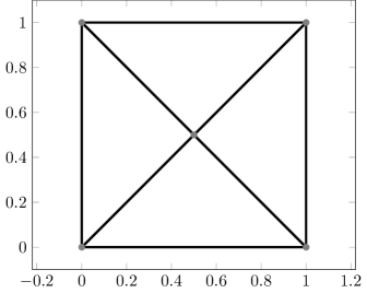
Figure 1. Initial mesh configuration of $\Omega=(0,1)^{2}$ with four triangles.

Throughout, we consider the convex domain $\Omega=(0,1)^{2}$ and the manufactured solution

$$u(t;x,y):=e^{-2\pi^{2}t}\sin(\pi x)\sin(\pi y).$$

Note that $u$ is smooth and its trace vanishes on $\Gamma=\partial\Omega$. Moreover, we choose $\boldsymbol{A}$ to be the identity matrix, $\boldsymbol{\beta}(x,y)=(1,1)^{T}$, $\gamma(x,y)=0$ for $(x,y)\in\Omega$. In subsection 5.1 we consider the solutions of Eq. 7, where the right-hand side data $f$ is given through Eq. 3, i.e., $f:=\dot{u}-\Delta u-\boldsymbol{\beta}\cdot\nabla u$. Also note that by Eq. 3 we have ${\boldsymbol{\sigma}}=\nabla u$. In subsection 5.2 we consider the solutions of Eq. 28, where the right-hand side data $f$ is given through Eq. 26, i.e., $f=\dot{u}-\Delta u+\boldsymbol{\beta}\cdot\nabla u$. Furthermore, in this case ${\boldsymbol{\sigma}}=\nabla u-\boldsymbol{\beta}u$.

In the following examples we use a lowest-order discretization, i.e., $p=0$. In order to obtain the optimal possible rates we have to consider two cases: For optimal rates for the scalar variable in the $L^{2}(\Omega)$ norm we have to equilibrate the time step ${k}$ and the mesh-size $h$ so that ${k}\simeq h^{2}$. If we are only interested in optimal rates for the error in the natural norm $\|\cdot\|_{{k}}$, it suffices to choose ${k}\simeq h$.

The problem set-up is quite simple: We choose as end time $T=0.1$. For all computations we start with an initial triangulation of $\Omega$ into four (similar) triangles, see Figure 1, and an initial time step ${k}=0.1$. We then solve Eq. 7, see subsection 5.1, resp. Eq. 28, see subsection 5.2. In the next step we refine the triangulation uniformly, i.e., each triangle is divided into four son triangles (by Newest Vertex Bisection). In our configuration this leads to four triangles which have diameter exactly half of their father triangle, i.e., $h/2$. Depending on which case we consider we then halve or quarter the time step, which ensures that either ${k}\simeq h$ or ${k}\simeq h^{2}$.

The initial data $u_{h}^{0}$ is chosen to be the $L^{2}$-projection of $u^{0}=u(0,\cdot)$ onto $\mathcal{S}_{0}^{1}(\mathcal{T})$. Note that $u$ is smooth (for all times), so that the initial data satisfies Eq. 22 and Eq. 23.

In all figures, we plot the errors that correspond to approximations of $u^{N}=u(T,\cdot)$, resp., ${\boldsymbol{\sigma}}^{N}={\boldsymbol{\sigma}}(T,\cdot)$ over the number of degrees of freedom in $U_{h}$. To that end define the following error quantities

$$\operatorname{err}(u_{h}^{N}) :=\|u^{N}-u_{h}^{N}\|,$$

$$\operatorname{err}(\nabla u_{h}^{N}) :=\|\nabla(u^{N}-u_{h}^{N})\|,$$

$$\operatorname{err}({\boldsymbol{\sigma}}_{h}^{N}) :=\|{\boldsymbol{\sigma}}^{N}-{\boldsymbol{\sigma}}_{h}^{N}\|,$$

$$\operatorname{err}({\rm div\,}{\boldsymbol{\sigma}}_{h}^{N}) :=\|{\rm div\,}({\boldsymbol{\sigma}}^{N}-{\boldsymbol{\sigma}}_{h}^{N})\|.$$

Triangles in the plots visualize the order of convergence, i.e., their negative slope $\alpha$ corresponds to $\mathcal{O}(h^{\alpha})$.

5.1. Example 1

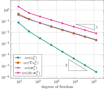
Figure 2. Example from subsection 5.1 with ${k}\simeq h^{2}$.

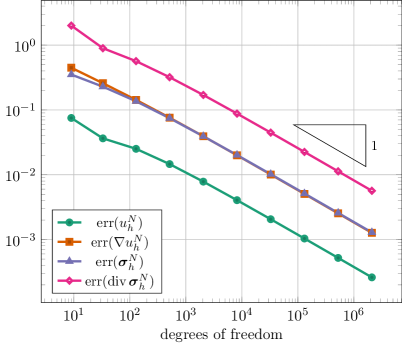
Figure 3. Example from subsection 5.1 with ${k}\simeq h$.

We consider the solutions $\boldsymbol{u}_{h}^{N}=(u_{h}^{N},{\boldsymbol{\sigma}}_{h}^{N})\in U_{h}$ of Eq. 7. Figure 2 shows the error quantities in the case where ${k}\simeq h^{2}$. By Theorem 8 we expect that $\operatorname{err}(u_{h}^{N})\lesssim h^{2}$. This is also observed in Figure 2. Note that the other quantities converge at a lower rate. In particular, observe that $\operatorname{err}({\rm div\,}{\boldsymbol{\sigma}}_{h}^{N})$ converges at the same rate as $\operatorname{err}({\boldsymbol{\sigma}}_{h}^{N})$, although from our analysis (Theorem 10) we can only infer that

$$\|\boldsymbol{u}^{N}-\boldsymbol{u}_{h}^{N}\|_{{k}}\simeq\operatorname{err}(\nabla u_{h}^{N})+\operatorname{err}({\boldsymbol{\sigma}}_{h}^{N})+{k}^{1/2}\operatorname{err}({\rm div\,}{\boldsymbol{\sigma}}_{h}^{N})=\mathcal{O}(h+{k})=\mathcal{O}(h+h^{2})=\mathcal{O}(h).$$

The results for the case where ${k}\simeq h$ are displayed in Figure 3. We observe that all error quantities, including $\operatorname{err}(u_{h}^{N})=\|u^{N}-u_{h}^{N}\|$, converge at the same rate. We conclude that it is not only sufficient but in general also necessary to set ${k}\simeq h^{2}$ to obtain higher rates for the $L^{2}$ error $\operatorname{err}(u_{h}^{N})$. As before we see that $\operatorname{err}({\rm div\,}{\boldsymbol{\sigma}}_{h}^{N})$ converges even at a higher rate than expected.

5.2. Example 2

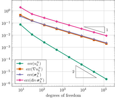
Figure 4. Example from subsection 5.2 with ${k}\simeq h^{2}$.

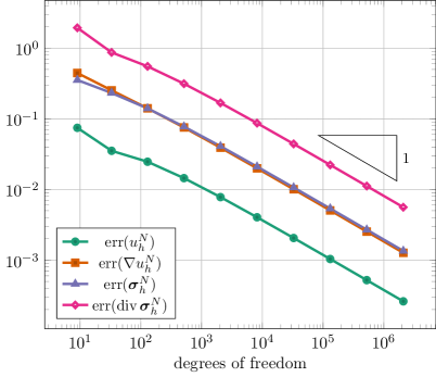
Figure 5. Example from subsection 5.2 with ${k}\simeq h$.

We consider the solutions $\boldsymbol{u}_{h}^{N}=(u_{h}^{N},{\boldsymbol{\sigma}}_{h}^{N})\in U_{h}$ from Eq. 28. Figures 4 and 5 show the error quantities in the cases ${k}\simeq h^{2}$ and ${k}\simeq h$, respectively. We make the same observations as in subsection 5.1.

References

- [1] P. B. Bochev and M. D. Gunzburger. Least-squares finite element methods, volume 166 of Applied Mathematical Sciences. Springer, New York, 2009.
- [2] Z. Cai and J. Ku. The norm error estimates for the div least-squares method. SIAM J. Numer. Anal., 44(4):1721–1734, 2006.
- [3] Z. Cai, R. Lazarov, T. A. Manteuffel, and S. F. McCormick. First-order system least squares for second-order partial differential equations. I. SIAM J. Numer. Anal., 31(6):1785–1799, 1994.
- [4] L. C. Evans. Partial differential equations, volume 19 of Graduate Studies in Mathematics. American Mathematical Society, Providence, RI, 1998.
- [5] P. Grisvard. Elliptic problems in nonsmooth domains, volume 24 of Monographs and Studies in Mathematics. Pitman (Advanced Publishing Program), Boston, MA, 1985.
- [6] M. Majidi and G. Starke. Least-squares Galerkin methods for parabolic problems. I. Semidiscretization in time. SIAM J. Numer. Anal., 39(4):1302–1323, 2001.
- [7] M. Majidi and G. Starke. Least-squares Galerkin methods for parabolic problems. II. The fully discrete case and adaptive algorithms. SIAM J. Numer. Anal., 39(5):1648–1666, 2001/02.
- [8] P.-A. Raviart and J. M. Thomas. A mixed finite element method for 2nd order elliptic problems. Springer, Berlin, 1977.
- [9] H. Rui, S. D. Kim, and S. Kim. Split least-squares finite element methods for linear and nonlinear parabolic problems. J. Comput. Appl. Math., 223(2):938–952, 2009.
- [10] L. R. Scott and S. Zhang. Finite element interpolation of nonsmooth functions satisfying boundary conditions. Math. Comp., 54(190):483–493, 1990.
- [11] V. Thomée. Galerkin finite element methods for parabolic problems, volume 25 of Springer Series in Computational Mathematics. Springer-Verlag, Berlin, second edition, 2006.
- [12] M. F. Wheeler. A priori error estimates for Galerkin approximations to parabolic partial differential equations. SIAM J. Numer. Anal., 10:723–759, 1973.
- [13] D.-P. Yang. Some least-squares Galerkin procedures for first-order time-dependent convection-diffusion system. Comput. Methods Appl. Mech. Engrg., 180(1-2):81–95, 1999.
- [14] D.-P. Yang. Analysis of least-squares mixed finite element methods for nonlinear nonstationary convection-diffusion problems. Math. Comp., 69(231):929–963, 2000.