Anderson accelerated fixed-stress splitting schemes for consolidation of unsaturated porous media

Abstract

In this paper, we study the robust linearization of nonlinear poromechanics of unsaturated materials. The model of interest couples the Richards equation with linear elasticity equations, employing the equivalent pore pressure. In practice a monolithic solver is not always available, defining the requirement for a linearization scheme to allow the use of separate simulators, which is not met by the classical Newton method. We propose three different linearization schemes incorporating the fixed-stress splitting scheme, coupled with an L-scheme, Modified Picard and Newton linearization of the flow. All schemes allow the efficient and robust decoupling of mechanics and flow equations. In particular, the simplest scheme, the Fixed-Stress-L-scheme, employs solely constant diagonal stabilization, has low cost per iteration, and is very robust. Under mild, physical assumptions, it is theoretically shown to be a contraction. Due to possible break-down or slow convergence of all considered splitting schemes, Anderson acceleration is applied as post-processing. Based on a special case, we justify theoretically the general ability of the Anderson acceleration to effectively accelerate convergence and stabilize the underlying scheme, allowing even non-contractive fixed-point iterations to converge. To our knowledge, this is the first theoretical indication of this kind. Theoretical findings are confirmed by numerical results. In particular, Anderson acceleration has been demonstrated to be very effective for the considered Picard-type methods. Finally, the Fixed-Stress-Newton scheme combined with Anderson acceleration provides a robust linearization scheme, meeting the above criteria.

1 Introduction

The coupling of fluid flow and mechanical deformation in unsaturated porous media is relevant for many applications ranging from modeling rainfall-induced land subsidence or levee failure to understanding the swelling and drying-shrinkage of wooden or cement-based materials. Assuming linear elastic behavior, the process can be modeled by coupling the Richards equations with quasi-static linear elasticity equations, generalizing the classical Biot equations [1]. In this work, we consider utilize the equivalent pore pressure [2], which allows a thermodynamically stable formulation [3].

For the numerical simulation of large scale applications, the solution of linear problems is typically the computationally most expensive component. For nonlinear problems, the dominating cost is determined by both the chosen linearization scheme and solver technology. In particular, the choice of a linearization scheme defines the requirements for the solver technology. Commonly, Newton’s method is the first choice linearization scheme. However, for the nonlinear Biot equations, as monolithic solver, Newton’s method requires the solver technology to solve saddle point problems coupling mechanics and flow equations. Additionally, in practice, constitutive laws employed in the model might be not Lipschitz continuous [4]. Thus, the arising systems are ill-conditioned and require an advanced, monolithic simulator. As the latter might be not available, the goal of this work is to develop a linearization scheme, which is robust and allows the use of decoupled simulators for mechanics and flow equations. For this purpose, we adopt closely related concepts for the linear Biot equations and the Richards equations.

For the numerical solution of the linear Biot equations, splitting schemes are widely used; either as iterative solvers [5] or as preconditioners [6]. In particular, the fixed-stress splitting scheme has aroused much interest, being unconditionally stable in the sense of a von Neumann analysis [7] and a global contraction [8, 9, 10]. As iterative solver, the scheme has been extended in various ways; e.g., it can be rewritten to a parallel-in-time solver [11], a multi-scale version allowing separate grids for the mechanics and flow problem has been developed [12], and the concept has been extended to nonlinear multi-phase flow coupled with linear elasticity [3]. In the context of monolithic solvers, the scheme has been applied as preconditioner for Krylov subspace methods [13, 14, 15, 16] and as smoother for multigrid methods [17]. All in all, the scheme defines a promising strategy to decouple mechanics and flow equations.

For the linearization of the Richards equation, the standard Newton method has to be used with care, since the Richards equation is a degenerate elliptic-parabolic equation, modeling saturated/unsaturated flow, and additionally material laws might be Hölder continuous. Various problem-specific alternatives have been developed in the literature. We want to point out two particular, simple linearization schemes; the L-scheme and the Modified Picard method. The L-scheme [18], employs diagonal stabilization for monotone, Lipschitz continuous nonlinearities. Global convergence has been rigorously proven for several porous media applications [19, 20, 21]; in particular also for the Richards equation [22]. The L-scheme can be also applied for Hölder continuous problems [21, 23]. Furthermore, for the Richards equations it can be used to define a robust, linear domain decomposition method [24]. The L-scheme linearization has been coupled with the fixed-stress splitting scheme for nonlinear Biot’s equations with linear coupling [25]. Less robust, but in some cases more efficient is the Modified Picard method [26], which employs the first order Taylor approximation for the saturation, still allowing for a Hölder continuous permeability.

In this paper, we combine the fixed-stress splitting scheme with the L-scheme, the Modified Picard method and Newton’s method. The resulting schemes decouple and linearize simultaneously the mechanics and flow equations, utilizing only a single loop and allowing for separate simulators. We show theoretically linear convergence of the Fixed-Stress-L-scheme, assuming non-vanishing residual saturation, permeability and porosity. However, the theoretical convergence rate might deteriorate in unfavorable situations, leading to either slow convergence or even stagnation in practice. As remedy we apply Anderson acceleration.

Anderson acceleration, originally introduced by [27], in order to accelerate fixed point iterations in electronic structure computation, has been successfully applied in various other fields; in particular for the modified Picard iteration [28]. Reusing previous iterations to approximate directional derivatives it can be related to a multi-secant quasi-Newton method [29] and to preconditioned GMRES for linear problems [30]. For nonlinear problems, it naturally generalizes to a preconditioned nonlinear GMRES. Being a post-processing, it can be combined with splitting methods, still allowing separate simulators unlike preconditioned monolithic solvers. So far, theoretical results guarantee only convergence for contractive fixed-point iterations [31]. Furthermore, those results do not guarantee actual acceleration. Based on a special case, we justify theoretically the ability of the Anderson acceleration to effectively accelerate convergence of contractive fixed-point iterations and moreover stabilize non-contractive fixed-point iterations. Applying Anderson acceleration for diverging methods might allow convergence after all. To our knowledge, this is the first theoretical indication of this kind. Other stabilization techniques could be applied as adaptive step size control, adaptive time stepping or the combination of a Picard-type method with a Newton-type method, following ideas by [32]. These concepts have not been considered in the scope of this work.

We present numerical results confirming the theoretical findings of this work. Indeed, the Fixed-Stress-L-scheme is more robust than the modifications employing Newton’s method and the Modified Picard method. Moreover, convergence of the Picard-type methods can be significantly accelerated by the Anderson acceleration. When applied to initially diverging methods, convergence can be reliably retained.

The main, new contributions of this work are:

• We propose three linearization schemes incorporating the fixed-stress splitting scheme, coupled with an L-scheme, Modified Picard and Newton linearization of the flow. All schemes allow the efficient and robust decoupling of mechanics and flow equations. For the simplest scheme, the Fixed-Stress-L-scheme, we show theoretical convergence, assuming non-vanishing residual saturation, permeability and porosity, cf. Theorem 7.

• Based on a special case, we justify theoretically the general ability of the Anderson acceleration to effectively accelerate convergence and stabilize the underlying scheme, allowing even non-contractive fixed-point iterations to converge, cf. Section 7.3.

• The combination of the proposed linearization schemes and Anderson acceleration is demonstrated numerically to be robust and efficient. In particular, Anderson acceleration allows the schemes to converge in challenging situations. The Fixed-Stress-Newton method coupled with Anderson acceleration shows best performance among the splitting schemes, cf. Section 8.

The paper is organized as follows. In Section 2, the mathematical model for the nonlinear Biot equations is explained. In Section 3, a three-field discretization is introduced, employing linear Galerkin finite elements and mixed finite element for the mechanics and flow equations, respectively. In Section 4, we recall the monolithic Newton method and introduce three splitting schemes, simultaneously linearizing and decoupling the mechanics and flow equations. In Section 5, convergence is proved for the Fixed-Stress-L-scheme. In Section 6, Anderson acceleration is recalled, and in Section 7, the ability of the Anderson acceleration to effectively accelerate convergence and increase robustness is discussed theoretically. In Section 8, numerical results are presented, illustrating in particular the increase of robustness via Anderson acceleration. The work is closed with concluding remarks in Section 9.

2 Mathematical model – Nonlinear Biot’s equations coupling Richards equation and linear elasticity

We consider a nonlinear extension of the classical, linear Biot equations modeling flow in deformable porous media under possibly both fully and partially saturated conditions. Further more we assume:

• The bulk material is linearly elastic and deforms solely under infinitesimal deformations.

• There exists two fluid phases – one active and one passive phase (standard assumption for the Richards equation).

• The active fluid phase is incompressible and corresponding fluxes are described by Darcy’s law.

• Mechanical inertia effects are negligible allowing to consider the quasi-static balance of linear momentum.

We model the medium at initial conditions by a reference configuration $\Omega\subset\mathbb{R}^{d}$, $d\in\{2,3\}$. Due to the limitation to infinitesimal deformations, the domain of the primary fields is approximated by $\Omega$ on the entire time interval of interest $(0,T)$, with final time $T>0$.

Finally, the governing equations describing coupled fluid flow and mechanical deformation of a porous medium with mechanical displacement $\bm{u}$, fluid pressure $p_{\mathrm{w}}$ and volumetric flux $\bm{q}_{\mathrm{w}}$ as primary variables are given by

$$\partial_{t}\left(\phi s_{\mathrm{w}}\right)+\bm{\nabla}\cdot\bm{q}_{\mathrm{w}} \,=\,0,$$ (1)

$$\bm{q}_{\mathrm{w}}+k_{\mathrm{w}}(s_{\mathrm{w}})\left(\bm{\nabla}p_{\mathrm{w}}-\rho_{\mathrm{w}}\bm{g}\right) \,=\,\bm{0},$$ (2)

$$-\bm{\nabla}\cdot\left[2\mu\bm{\varepsilon}(\bm{u})+\lambda\bm{\nabla}\cdot\bm{u}\bm{I}-\alpha p_{\mathrm{E}}(p_{\mathrm{w}})\bm{I}\right] \,=\,\rho_{\mathrm{b}}\bm{g},$$ (3)

where $\phi$ denotes variable porosity, $s_{\mathrm{w}}$ denotes fluid saturation, $k_{\mathrm{w}}$ denotes fluid-dependent mobility, $\rho_{\mathrm{w}}$ and $\rho_{\mathrm{b}}$ denote fluid and bulk density, respectively, $\bm{g}$ is the gravitational acceleration, $\bm{\varepsilon}(\bm{u})$ and $\bm{\nabla}\cdot\bm{u}$ denote the linear strain and the volumetric deformation, respectively, $\mu$ and $\lambda$ denote the Lamé parameters, $\alpha$ is the Biot coefficient and $p_{\mathrm{E}}$ denotes the pore pressure. In the following, we comment briefly on the single components of the mathematical model and refer to [2] for a detailed derivation.

• For the fluid flow, an active and a passive fluid phase are assumed. In other words, the passive phase responds instantaneously to the active phase and therefore has a constant pressure. The behavior of the active fluid phase is governed by mass conservation, identical to volume conservation for an incompressible fluid. The volume is given by the product of porosity $\phi$ and saturation $s_{\mathrm{w}}$. The porosity changes linearly with volumetric deformation $\bm{\nabla}\cdot\bm{u}$ and pore pressure $p_{\mathrm{E}}$ by

  $$\phi(\bm{u},p_{\mathrm{w}})\,=\,\phi_{0}+\alpha\bm{\nabla}\cdot(\bm{u}-\bm{u}_{0})+\frac{1}{N}(p_{\mathrm{E}}(p_{\mathrm{w}})-p_{\mathrm{E}}(p_{\mathrm{w},0})),$$ (4)

  where $\phi_{0}$, $\bm{u}_{0}$ and $p_{\mathrm{w},0}$ are the initial porosity, displacement and pressure, respectively, and $\alpha$ is the Biot coefficient and $N$ is the Biot modulus. Eq. (4) is a byproduct of the thermodynamic derivation of the effective stress by Coussy [2]. Furthermore, the saturation $s_{\mathrm{w}}=s_{\mathrm{w}}(p)$ is assumed to be described by a material law $s_{\mathrm{w}}:\mathbb{R}\rightarrow(0,1]$, satisfying $s_{\mathrm{w}}(p)=1$, $p\geq 0$, and having a negative inverse $p_{\mathrm{c}}:(0,1]\rightarrow\mathbb{R}_{+}$, satisfying $s_{\mathrm{w}}(-p_{\mathrm{c}}(s))=s$, $s\in(0,1]$. In the literature, the function $p_{\mathrm{c}}$ is often referred to as capillary pressure.

• The volumetric flux $\bm{q}_{\mathrm{w}}$ is assumed to be described by Darcy’s law for multiphase flow. Here, the permeability scaled by viscosity is given by a material law $k_{\mathrm{w}}=k_{\mathrm{w}}(s_{\mathrm{w}})$. In practice, the material laws can become Hölder continuous.

• The mechanical behavior is governed by balance of linear momentum under quasi-static conditions, combined with an effective stress formulation. Allowing only for small deformations, we employ the St.Venant Kirchhoff model for the effective stress, determining the poroelastic stress as $\bm{\sigma}^{\mathrm{por}}(\bm{u},p_{\mathrm{w}})=2\mu\bm{\varepsilon}(\bm{u})+\lambda\bm{\nabla}\cdot\bm{u}\bm{I}-\alpha p_{\mathrm{E}}(p_{\mathrm{w}})$. As pore pressure, we use the equivalent pore pressure [2]

  $$p_{\mathrm{E}}(p)\,=\,s_{\mathrm{w}}(p)p-\int_{s_{\mathrm{w}}(p)}^{1}p_{\mathrm{c}}(s)\,ds,$$ (5)

  which takes into account interfacial effects. By construction it satisfies $dp_{\mathrm{E}}=s_{\mathrm{w}}(p)\,dp$. As body force we assume solely gravity, where for the sake of simplicity the bulk density $\rho_{\mathrm{b}}$ is assumed to be constant. All in all, Eq. (3) acts as compatibility condition to be satisfied at each time.

Introducing two partitions $\Gamma_{D}^{f}\cup\Gamma_{N}^{f}=\Gamma_{D}^{m}\cup\Gamma_{N}^{m}=\partial\Omega$ of the boundary of $\Omega$ and the outer normal $\bm{n}$ on $\partial\Omega$, we assume boundary conditions and initial conditions

$$p_{\mathrm{w}} =p_{w,D} \text{on }\Gamma_{D}^{f}\times(0,T), \bm{u} =\bm{u}_{D} \text{on }\Gamma_{D}^{m}\times(0,T),$$

$$\bm{q}_{\mathrm{w}}\cdot\bm{n} =\bm{q}_{w,N} \text{on }\Gamma_{N}^{f}\times(0,T), \bm{\sigma}^{\mathrm{por}}(\bm{u},p_{\mathrm{w}})\bm{n} =\bm{\sigma}^{\mathrm{por}}_{n} \text{on }\Gamma_{N}^{m}\times(0,T),$$

$$p_{\mathrm{w}} =p_{\mathrm{w},0} \text{in }\Omega\times\{0\}, \bm{u} =\bm{u}_{0} \text{in }\Omega\times\{0\}.$$

All in all, the nonlinear Biot equations (1)–(3) couple nonlinearly the Richards equation and linear elasticity equations. In the fully saturated regime ($p_{\mathrm{w}}\geq 0$), the model reduces locally to the classical, linear Biot equations for an incompressible fluid and compressible rock. We note, as long as the fluid saturation is not vanishing, the nonlinear Biot equations (1)–(3) are parabolic, unlike the degenerate elliptic-parabolic Richards equation, cf. Remark 3.

3 Finite element discretization

We discretize the Biot equations (1)–(3) in space and time by the finite element method and the implicit Euler method, respectively. More precisely, given a regular triangulation $\mathcal{T}_{h}$ of the domain $\Omega$, we employ linear, constant and lowest order Raviart-Thomas finite elements to approximate displacement, pressure and volumetric flux, respectively. For the sake of simplicity, we assume zero boundary conditions on $\partial\Omega=\Gamma_{D}^{m}=\Gamma_{D}^{f}$. The corresponding discrete function spaces are then given by

$$W_{h} \,=\,\Bigl{\{}w_{h}\in L^{2}(\Omega)\,\Bigm{|}\,\forall T\in\mathcal{T}_{h},w_{h}|_{T}\in{{\mathbb{P}}_{0}}\Bigr{\}},$$

$$\bm{Z}_{h} \,=\,\Bigl{\{}\bm{z}_{h}\in{H(\mathrm{div};\Omega)}\,\Bigm{|}\,\forall T\in\mathcal{T}_{h},\bm{z}_{h}|_{T}(\bm{x})=\bm{a}+b\bm{x},\ \bm{a}\in\mathbb{R}^{d},b\in\mathbb{R}\Bigr{\}},$$

$$\bm{V}_{h} \,=\,\Bigl{\{}\bm{v}_{h}\in{[H^{1}_{0}(\Omega)]}^{d}\,\Bigm{|}\,\forall T\in\mathcal{T}_{h},\bm{v}_{h}|_{T}\in{[{\mathbb{P}}_{1}]}^{d}\Bigr{\}},$$

where ${\mathbb{P}}_{0}$ and ${\mathbb{P}}_{1}$ denote the spaces of scalar piecewise constant and piecewise (bi-)linear functions, respectively, and elements of $\bm{V}_{h}$ are zero on the boundary. We note, that the chosen discretization is not stable with respect to the full range of material parameters [33], e.g., for very small permeability. However, the specific choice of the finite element spaces is not essential for the further discussion of the linearization. Furthermore, for the temporal discretization we employ a partition $\{t^{n}\}_{n}$ of the time interval $(0,T)$ with (constant) time step size $\tau=t^{n}-t^{n-1}>0$.

Then given initial data $(p,\bm{u})_{h}^{0}\in W_{h}\times\bm{V}_{h}$, at each time step $n\geq 1$, the discrete problem reads: Given $(p,\bm{q},\bm{u})_{h}^{n-1}\in W_{h}\times\bm{Z}_{h}\times\bm{V}_{h}$, find $(p,\bm{q},\bm{u})_{h}^{n}\in W_{h}\times\bm{Z}_{h}\times\bm{V}_{h}$, satisfying for all $(w,\bm{z},\bm{v})_{h}\in W_{h}\times\bm{Z}_{h}\times\bm{V}_{h}$

$$\langle\phi^{n-1}(s_{\mathrm{w}}^{n}-s_{\mathrm{w}}^{n-1}),w_{h}\rangle+\alpha\langle s_{\mathrm{w}}^{n}\bm{\nabla}\cdot(\bm{u}_{h}^{n}-\bm{u}_{h}^{n-1}),w_{h}\rangle+\tfrac{1}{N}\langle s_{\mathrm{w}}^{n}(p_{\mathrm{E}}^{n}-p_{\mathrm{E}}^{n-1}),w_{h}\rangle+\tau\langle\bm{\nabla}\cdot\bm{q}_{h}^{n},w_{h}\rangle \,=\,0,$$ (6)

$$\langle k_{\mathrm{w}}(s_{\mathrm{w}}^{n})^{-1}\bm{q}_{h}^{n},\bm{z}_{h}\rangle-\langle p_{h}^{n},\bm{\nabla}\cdot\bm{z}_{h}\rangle \,=\,\langle\rho_{\mathrm{w}}\bm{g},\bm{z}_{h}\rangle,$$ (7)

$$2\mu\langle\bm{\varepsilon}(\bm{u}_{h}^{n}),\bm{\varepsilon}(\bm{v}_{h})\rangle+\lambda\langle\bm{\nabla}\cdot\bm{u}_{h}^{n},\bm{\nabla}\cdot\bm{v}_{h}\rangle-\alpha\langle p_{\mathrm{E}}^{n},\bm{\nabla}\cdot\bm{v}_{h}\rangle \,=\,\langle\rho_{\mathrm{b}}\bm{g},\bm{v}_{h}\rangle,$$ (8)

where $s_{\mathrm{w}}^{k}=s_{\mathrm{w}}(p_{h}^{k})$ and $p_{\mathrm{E}}^{k}=p_{\mathrm{E}}(p_{h}^{k})$, $k\in\{n-1,n\}$ and $\phi^{n-1}=\phi(\bm{u}_{h}^{n-1},p_{h}^{n-1})$. Here, $\langle\cdot,\cdot\rangle$ denotes the standard $L^{2}(\Omega)$ scalar product.

Remark 1 (Volume conservation).

The discretization (6)–(8) is volume-conservative as by Eq. (4) it holds

$$\phi^{n}s_{\mathrm{w}}^{n}-\phi^{n-1}s_{\mathrm{w}}^{n-1} \,=\,\phi^{n-1}(s_{\mathrm{w}}^{n}-s_{\mathrm{w}}^{n-1})+s_{\mathrm{w}}^{n}\left(\alpha\bm{\nabla}\cdot(\bm{u}^{n}-\bm{u}^{n-1})+\frac{1}{N}(p_{\mathrm{E}}^{n}-p_{\mathrm{E}}^{n-1})\right).$$

4 Monolithic and decoupled linearization schemes

In the following, we consider four linearization schemes. First, we apply the monolithic Newton method, being commonly the first choice when linearizing a nonlinear problem. Second, we propose a linearization scheme, which employs constant diagonal stabilization in order to linearize and decouple simultaneously the mechanics and flow equations. Furthermore, we introduce two modifications of the latter method, utilizing both decoupling and first order Taylor approximations. For direct comparison, we formulate all schemes in incremental form.

Monolithic schemes vs. iterative operator splitting schemes for saddle point problems

Biot’s equations yield a saddle point problem, which in general are difficult to solve. Containing more information on coupling terms, a monolithic scheme for this purpose is per se more stable, whereas for iterative operator splitting schemes, stability is always an issue necessary to be checked. However, in contrast to robust splitting schemes, for a monolithic scheme a fully coupled simulator with advanced solver technology is required. For that, one possibility is to apply a splitting scheme as either an iterative solver or a preconditioner for a Krylov subspace method. The latter is more efficient and robust, cf. e.g. [13] for the linear Biot equations. In case only separate simulators are available, the concept of preconditioning the coupled problem cannot be applied in the same sense. But we note that acceleration techniques as Anderson acceleration can be applied as post-processing to the iterative splitting schemes, acting as preconditioned nonlinear GMRES solvers applied to the coupled problem, cf. Section 6.

4.1 Notation of residuals

For the incremental formulation of the linearization schemes, we introduce naturally defined residuals of the coupled problem (1)–(3). Given data $(p,\bm{q},\bm{u})_{h}^{n-1}\in W_{h}\times\bm{Z}_{h}\times\bm{V}_{h}$ for time step $n-1$, the residuals at time step $n$ evaluated at some state $(p,\bm{q},\bm{u})_{h}\in W_{h}\times\bm{Z}_{h}\times\bm{V}_{h}$ and tested with $(w,\bm{z},\bm{v})_{h}\in W_{h}\times\bm{Z}_{h}\times\bm{V}_{h}$ are defined by

$$r_{p}^{n}((p,\bm{q},\bm{u})_{h};w_{h}) =-\Big{(}\langle\phi^{n-1}(s_{\mathrm{w}}(p_{h})-s_{\mathrm{w}}^{n-1}),w_{h}\rangle+\alpha\langle s_{\mathrm{w}}(p_{h})\bm{\nabla}\cdot(\bm{u}_{h}-\bm{u}_{h}^{n-1}),w_{h}\rangle$$

$$\quad\qquad+\frac{1}{N}\langle s_{\mathrm{w}}(p_{h})(p_{\mathrm{E}}(p_{h})-p_{\mathrm{E}}^{n-1}),w_{h}\rangle+\tau\langle\bm{\nabla}\cdot\bm{q}_{h},w_{h}\rangle\Big{)},$$

$$r_{q}^{n}((p,\bm{q},\bm{u})_{h};\bm{z}_{h}) =\langle\rho_{\mathrm{w}}\bm{g},\bm{z}_{h}\rangle-\Big{(}\langle k_{\mathrm{w}}(s_{\mathrm{w}}(p_{h}))^{-1}\bm{q}_{h},\bm{z}_{h}\rangle-\langle p_{h},\bm{\nabla}\cdot\bm{z}_{h}\rangle\Big{)},$$

$$r_{u}^{n}((p,\bm{q},\bm{u})_{h};\bm{v}_{h}) =\langle\rho_{\mathrm{b}}\bm{g},\bm{v}_{h}\rangle-\Big{(}2\mu\langle\bm{\varepsilon}(\bm{u}_{h}),\bm{\varepsilon}(\bm{v}_{h})\rangle+\lambda\langle\bm{\nabla}\cdot\bm{u}_{h},\bm{\nabla}\cdot\bm{v}_{h}\rangle-\alpha\langle p_{\mathrm{E}}(p_{h}),\bm{\nabla}\cdot\bm{v}_{h}\rangle\Big{)}.$$

Shorter, given a sequence of approximations $(p,\bm{q},\bm{u})_{h}^{n,i}\in W_{h}\times\bm{Z}_{h}\times\bm{V}_{h}$, $i\in\mathbb{N}$, of $(p,\bm{q},\bm{u})_{h}^{n}\in W_{h}\times\bm{Z}_{h}\times\bm{V}_{h}$, we define

$$r_{p}^{n,i}(w_{h}) \,=\,r_{p}^{n}((p,\bm{q},\bm{u})_{h}^{n,i};w_{h}),$$

$$r_{q}^{n,i}(\bm{z}_{h}) \,=\,r_{q}^{n}((p,\bm{q},\bm{u})_{h}^{n,i};\bm{z}_{h}),$$

$$r_{u}^{n,i}(\bm{v}_{h}) \,=\,r_{u}^{n}((p,\bm{q},\bm{u})_{h}^{n,i};\bm{v}_{h}),$$

$$r_{u}^{n,i/i-1}(\bm{v}_{h}) \,=\,r_{u}^{n}((p,\bm{q})_{h}^{n,i},\bm{u}_{h}^{n,i-1};\bm{v}_{h}).$$

4.2 Monolithic Newton’s method

We apply the standard Newton method linearizing the coupled problem (6)–(8) in a monolithic fashion.

Scheme

The monolithic Newton method reads: For each time step, given the initial guess $(p,\bm{q},\bm{u})_{h}^{n,0}=(p,\bm{q},\bm{u})_{h}^{n-1}$, loop over the iterations $i\in\mathbb{N}$ until convergence is reached. Given data at the previous time step $n-1$ and iteration $i-1$, find the increments $\varDelta(p,\bm{q},\bm{u})_{h}^{n,i}\in W_{h}\times\bm{Z}_{h}\times\bm{V}_{h}$, satisfying the coupled, linear problem, for all $(w,\bm{z},\bm{v})_{h}\in W_{h}\times\bm{Z}_{h}\times\bm{V}_{h}$,

$$\left\langle\left(\phi^{i-1}\frac{\partial s_{\mathrm{w}}}{\partial p_{\mathrm{w}}}(p_{h}^{n,i-1})+\frac{1}{N}(s_{\mathrm{w}}^{n,i-1})^{2}\right)\varDelta p_{h}^{n,i},w_{h}\right\rangle+\alpha\langle s_{\mathrm{w}}^{n,i-1}\bm{\nabla}\cdot\varDelta\bm{u}_{h}^{n,i},w_{h}\rangle+\tau\langle\bm{\nabla}\cdot\varDelta\bm{q}_{h}^{n,i},w_{h}\rangle \,=\,r_{p}^{n,i-1}(w_{h}),$$ (9)

$$\langle k_{\mathrm{w}}(s_{\mathrm{w}}^{n,i-1})^{-1}\varDelta\bm{q}_{h}^{n,i},\bm{z}_{h}\rangle+\left\langle\left(\left.\frac{\partial}{\partial p_{\mathrm{w}}}k_{\mathrm{w}}(s_{\mathrm{w}}^{n,i-1})\right|_{p_{h}^{n,i-1}}\right)^{-1}\bm{q}_{h}^{n,i-1}\varDelta p_{h}^{n,i},\bm{z}_{h}\right\rangle-\langle\varDelta p_{h}^{n,i},\bm{\nabla}\cdot\bm{z}_{h}\rangle \,=\,r_{q}^{n,i-1}(\bm{z}_{h}),$$ (10)

$$2\mu\langle\bm{\varepsilon}(\varDelta\bm{u}_{h}^{n,i}),\bm{\varepsilon}(\bm{v}_{h})\rangle+\lambda\langle\bm{\nabla}\cdot\varDelta\bm{u}_{h}^{n,i},\bm{\nabla}\cdot\bm{v}_{h}\rangle-\alpha\langle s_{\mathrm{w}}^{n,i-1}\varDelta p_{h}^{n,i},\bm{\nabla}\cdot\bm{v}_{h}\rangle \,=\,r_{u}^{n,i-1}(\bm{v}_{h}),$$ (11)

and set

$$(p,\bm{q},\bm{u})_{h}^{n,i}\,=\,(p,\bm{q},\bm{u})_{h}^{n,i-1}+\varDelta(p,\bm{q},\bm{u})_{h}^{n,i}.$$

After convergence is reached at iteration $N$, set $(p,\bm{q},\bm{u})_{h}^{n}=(p,\bm{q},\bm{u})_{h}^{n,N}$.

Properties

Newton’s method is known to be quadratically, locally convergent, which makes the method commonly the first choice linearization method. However, in general it is not robust and has the following drawbacks:

• In order to ensure convergence, the time step size has to be chosen sufficiently small depending on the mesh size. Then the initial guess is sufficiently close to the unknown solution.

• The need for a good initial guess can be relaxed by using step size control, allowing a bigger time step size. Anderson acceleration applied as post-processing can be interpreted as such, for more details, cf. Section 6.

• Bounded derivatives of constitutive laws have to be available. In practice, nonlinearities employed in the model (1)–(3) are not necessarily Lipschitz continuous, e.g., the relative permeability for soils. In particular, in the transition from the partially to the fully saturated regime, the derivative of the relative permeability modeled by the van Genuchten model [4] can be unbounded. Consequently, the Jacobian might become ill-conditioned.

• Due to the coupled nature of the problem, the linear system resulting from the problem (9)–(11) has a saddle point structure and is therefore ill-conditioned. Hence, an advanced solver architecture is required. In the context of Biot’s equations, the application of a fixed-stress type solver or preconditioner [13] yields remedy.

4.3 Fixed-Stress-L-scheme – A Picard-type simultaneous linearization and splitting

We propose a novel, robust linearization scheme for Eq. (6)–(8). It is essentially a simultaneous application of the L-scheme linearization for the Richards equation, cf. e.g. [22], and the fixed-stress splitting scheme for the linear Biot equations, cf. e.g. [7], both utilizing diagonal stabilization. In the following, we refer to the scheme as Fixed-Stress-L-scheme (FSL). As derived in Section 5, it can be interpreted as L-scheme linearization of the nonlinear Biot equations reduced to a pure pressure formulation or alternatively as nonlinear Gauss-Seidel-type solver, consisting of cheap iterations allowing separate, sophisticated simulators for the mechanical and flow subproblems. In Section 5, we show convergence of the Fixed-Stress-L-scheme under physical assumptions. Before defining the Fixed-Stress-L-scheme, we recall main ideas of both the L-scheme and the fixed-stress splitting scheme.

Main ideas of the L-scheme

The L-scheme is an inexact Newton’s method, employing constant linearization for monotone and Lipschitz continuous terms. For remaining contributions Picard-type linearization is applied. Effectively, this approach is identical with applying a Picard iteration with diagonal stabilization. All in all, no explicit derivatives are required at the price that only linear convergence can be expected. Under mild conditions, this concept has been rigorously proven to be globally convergent for various porous media applications, e.g., [22, 20, 21, 25]. Moreover, as pointed out by [22], the resulting linear problem is expected to be significantly better conditioned than the corresponding linear problem obtained by Newton’s method.

Regarding the nonlinear Biot equations, the saturation $s_{\mathrm{w}}=s_{\mathrm{w}}(p)$ is classically non-decreasing and Lipschitz continuous. Hence, assuming that $\phi^{i-1}\geq 0$ on $\Omega$, the above criteria apply to the saturation contribution in Eq. (9). The approximation of the saturation at iteration $i$ is then given by

$$s_{\mathrm{w}}^{n}\,=\,s_{\mathrm{w}}(p_{h}^{n})\,\approx\,s_{\mathrm{w}}(p_{h}^{n,i})\,\approx\,s_{\mathrm{w}}(p_{h}^{n,i-1})+L(p_{h}^{n,i}-p_{h}^{n,i-1})\,=\,s_{\mathrm{w}}(p_{h}^{n,i-1})+L\varDelta p_{h}^{n,i},$$ (12)

where $L\in\mathbb{R}_{+}$ is a sufficiently large tuning parameter, usually set equal to the Lipschitz constant $L_{\mathrm{s}}$ of $s_{\mathrm{w}}$. As coupling terms are not monotone, Picard-type linearization is applied to the remaining contributions of Eq. (6)–(8).

Main ideas of the fixed-stress splitting scheme

Considering the linear Biot equations, their linearization results in a saddle point problem, thus, requiring an advanced solver technology for efficient solution. For this purpose, physically motivated, robust, iterative splitting schemes are widely-used as, e.g., the fixed-stress splitting scheme, originally introduced by [5]. As it decouples mechanics and flow equations, separate simulators can be utilized for both subproblems, reducing the complexity to solving simpler, better conditioned problems. The robust decoupling is accomplished via sufficient diagonal stabilization, introducing a tuning parameter $\beta_{\mathrm{FS}}$. Its optimization with guaranteed convergence is a research question on its own [8, 9, 34]. Concepts can be also extended to multiphase flow coupled with linear elasticity [3].

Scheme

We observe that applying the monolithic L-scheme, as just explained to the nonlinear, discrete Biot equations (6)–(8), results in a linear problem equivalent with that for single phase flow in heterogeneous media, for which the fixed-stress splitting scheme is an attractive solver [9]. Both schemes are realized via diagonal stabilization. Anticipating the dynamics to be mainly governed by the flow problem, cf. Assumption (A4), and the mechanics problem to be much simpler, a simultaneous application of the L-scheme and the fixed-stress splitting scheme yields an attractive linearization scheme incorporating the decoupling of flow and mechanics equations.

Written as iterative scheme in incremental form, the resulting Fixed-Stress-L-scheme reads: For each time step, given the initial guess $(p,\bm{q},\bm{u})_{h}^{n,0}=(p,\bm{q},\bm{u})_{h}^{n-1}$, loop over the iterations $i\in\mathbb{N}$ until convergence is reached. For each iteration $i$, perform two steps:

1. Step: Set $L=L_{\mathrm{s}}$, the Lipschitz constant of $s_{\mathrm{w}}$, and $\beta_{\mathrm{FS}}=\alpha^{2}/\left(\tfrac{2\mu}{d}+\lambda\right)$. Given $(p,\bm{q},\bm{u})_{h}^{n,i-1},(p,\bm{q},\bm{u})_{h}^{n-1}\in W_{h}\times\bm{Z}_{h}\times\bm{V}_{h}$, find the increments $\varDelta(p,\bm{q})_{h}^{n,i}\in W_{h}\times\bm{Z}_{h}$, satisfying, for all $(w,\bm{z})_{h}\in W_{h}\times\bm{Z}_{h}$,

$$\left\langle\left(L+\tfrac{1}{N}+\beta_{\mathrm{FS}}\right)\varDelta p_{h}^{n,i},w_{h}\right\rangle+\tau\langle\bm{\nabla}\cdot\varDelta\bm{q}_{h}^{n,i},w_{h}\rangle \,=\,r_{p}^{n,i-1}(w_{h}),$$ (13)

$$\langle k_{\mathrm{w}}(s_{\mathrm{w}}^{n,i-1})^{-1}\varDelta\bm{q}_{h}^{n,i},\bm{z}_{h}\rangle-\langle\varDelta p_{h}^{n,i},\bm{\nabla}\cdot\bm{z}_{h}\rangle \,=\,r_{q}^{n,i-1}(\bm{z}_{h}),$$ (14)

and set

$$(p,\bm{q})_{h}^{n,i}\,=\,(p,\bm{q})_{h}^{n,i-1}+\varDelta(p,\bm{q})_{h}^{n,i}.$$

2. Step: Given $((p,\bm{q})_{h}^{n,i},\bm{u}_{h}^{n,i-1})\in W_{h}\times\bm{Z}_{h}\times\bm{V}_{h}$, find the increment $\varDelta\bm{u}_{h}^{n,i}\in\bm{V}_{h}$, satisfying, for all $\bm{v}_{h}\in\bm{V}_{h}$,

$$2\mu\langle\bm{\varepsilon}(\varDelta\bm{u}_{h}^{n,i}),\bm{\varepsilon}(\bm{v}_{h})\rangle+\lambda\langle\bm{\nabla}\cdot\varDelta\bm{u}_{h}^{n,i},\bm{\nabla}\cdot\bm{v}_{h}\rangle \,=\,r_{u}^{n,i/i-1}(\bm{v}_{h}),$$ (15)

and set

$$\bm{u}_{h}^{n,i} \,=\,\bm{u}_{h}^{n,i-1}+\varDelta\bm{u}_{h}^{n,i}.$$

After convergence is reached at iteration $N$, set $(p,\bm{q},\bm{u})_{h}^{n}=(p,\bm{q},\bm{u})_{h}^{n,N}$.

Properties

The Fixed-Stress-L-scheme inherits its properties from the underlying methods. It does not require the evaluation of any derivatives, increasing the speed of the assembly process. It is very robust but guarantees only linear convergence, as shown in Section 5, cf. Theorem 7. Furthermore, the Fixed-Stress-L-scheme requires solely the solution of the mechanical and flow problem, allowing separate simulators. In particular, the overall method utilizes a single loop in contrast to the Newton’s method combined with a fixed-stress splitting scheme as iterative solver.

4.4 Quasi-Newton modifications of the Fixed-Stress-L-scheme

The Fixed-Stress-L-scheme employs constant linearization for the fluid volume $\phi s_{\mathrm{w}}$ with respect to fluid pressure, utilizing an upper bound for the Lipschitz constant. In many practical situations, this approach is quite pessimistic. Recalling the assumption that the flow problem dominates the dynamics of the system, we expect the simultaneous application of the fixed-stress splitting scheme and more sophisticated flow linearizations to be only slightly less robust than the Fixed-Stress-L-scheme. Independent of the flow linearization, diagonal stabilization is added by the splitting scheme increasing the robustness. In the following, based on the derivation of the Fixed-Stress-L-scheme in Section 5, cf. Remark 4, we couple simultaneously a modified Picard method [26] and Newton’s method with the fixed-stress splitting scheme yielding the Fixed-Stress-Modified-Picard method and the Fixed-Stress-Newton method, respectively. The modified Picard method, in particular, is a widely-used linearization scheme for the Richards equation and hence rises interest for its use for the linearization of the discrete, nonlinear Biot equations (6)–(8).

Fixed-Stress-Modified-Picard method

Applied to the Richards equations, the modified Picard method employs a first order Taylor approximation as linearization for the saturation and a Picard-type linearization for the possibly Hölder continuous permeability. By employing a first order approximation of the fluid volume $\phi s_{\mathrm{w}}$ with respect to fluid pressure instead, and by coupling simultaneously with the fixed-stress splitting scheme, we obtain a linearization scheme for Eq. (6)–(8). For later reference, we denote the resulting scheme by Fixed-Stress-Modified-Picard-scheme. It is essentially identical with the Fixed-Stress-L-scheme but with modified first fixed-stress step (1. Step). We exchange Eq. (13)–(14) with

$$\left\langle\left(\phi^{i-1}\frac{\partial s_{\mathrm{w}}}{\partial p_{\mathrm{w}}}(p_{h}^{n,i-1})+\left(\tfrac{1}{N}+\beta_{\mathrm{FS}}\right)(s_{\mathrm{w}}^{n,i-1})^{2}\right)\varDelta p_{h}^{n,i},w_{h}\right\rangle+\tau\langle\bm{\nabla}\cdot\varDelta\bm{q}_{h}^{n,i},w_{h}\rangle \,=\,r_{p}^{n,i-1}(w_{h}),$$ (16)

$$\langle k_{\mathrm{w}}(s_{\mathrm{w}}^{n,i-1})^{-1}\varDelta\bm{q}_{h}^{n,i},\bm{z}_{h}\rangle-\langle\varDelta p_{h}^{n,i},\bm{\nabla}\cdot\bm{z}_{h}\rangle \,=\,r_{q}^{n,i-1}(\bm{z}_{h}).$$ (17)

Fixed-Stress-Newton method

In case the permeability is Lipschitz continuous, the simultaneous application of the fixed-stress splitting scheme and linearization of the flow equations via Newton’s method yields an attractive linearization scheme for Eq. (6)–(8). For later reference, we denote the resulting scheme by Fixed-Stress-Newton method. It is essentially identical with the Fixed-Stress-L-scheme but with modified first fixed-stress step (1. Step). We exchange Eq. (13)–(14) with

$$\left\langle\left(\phi^{i-1}\frac{\partial s_{\mathrm{w}}}{\partial p_{\mathrm{w}}}(p_{h}^{n,i-1})+\left(\tfrac{1}{N}+\beta_{\mathrm{FS}}\right)(s_{\mathrm{w}}^{n,i-1})^{2}\right)\varDelta p_{h}^{n,i},w_{h}\right\rangle+\tau\langle\bm{\nabla}\cdot\varDelta\bm{q}_{h}^{n,i},w_{h}\rangle \,=\,r_{p}^{n,i-1}(w_{h}),$$ (18)

$$\langle k_{\mathrm{w}}(s_{\mathrm{w}}^{n,i-1})^{-1}\varDelta\bm{q}_{h}^{n,i},\bm{z}_{h}\rangle+\left\langle\left(\left.\frac{\partial}{\partial p_{\mathrm{w}}}k_{\mathrm{w}}(s_{\mathrm{w}}^{n,i-1})\right|_{p_{h}^{n,i-1}}\right)^{-1}\bm{q}_{h}^{n,i-1}\varDelta p_{h}^{n,i},\bm{z}_{h}\right\rangle-\langle\varDelta p_{h}^{n,i},\bm{\nabla}\cdot\bm{z}_{h}\rangle \,=\,r_{q}^{n,i-1}(\bm{z}_{h}).$$ (19)

We note that the Fixed-Stress-Newton method is also closely related to applying a single fixed-stress iteration as inexact solver for the linear problem (9)–(11) arising from Newton’s method.

4.5 $L^{2}(\Omega)$-type stopping criterion

For the numerical examples in Section 8, we employ a combination of an absolute and a relative $L^{2}(\Omega)$-type stopping criterion, closely related to the standard algebraic $l^{2}$-type criterion. Given tolerances $\varepsilon_{\mathrm{a}},\ \varepsilon_{\mathrm{r}}\in\mathbb{R}_{+}$, we denote an iteration as converged if it holds

$$\|\varDelta p_{h}^{n,i}\|_{L^{2}(\Omega)}+\|\varDelta\bm{q}_{h}^{n,i}\|_{L^{2}(\Omega)}+\|\varDelta\bm{u}_{h}^{n,i}\|_{L^{2}(\Omega)}<\varepsilon_{\mathrm{a}},\qquad\text{and}\qquad\frac{\|\varDelta p_{h}^{n,i}\|_{L^{2}(\Omega)}}{\|p_{h}^{n,i}\|_{L^{2}(\Omega)}}+\frac{\|\varDelta\bm{q}_{h}^{n,i}\|_{L^{2}(\Omega)}}{\|\bm{q}_{h}^{n,i}\|_{L^{2}(\Omega)}}+\frac{\|\varDelta\bm{u}_{h}^{n,i}\|_{L^{2}(\Omega)}}{\|\bm{u}_{h}^{n,i}\|_{L^{2}(\Omega)}}<\varepsilon_{\mathrm{r}}.$$

5 Convergence theory for simultaneous linearization and splitting via the L-scheme

In the following, we show convergence of the Fixed-Stress-L-scheme (13)–(15) under mild, physical assumptions. For this purpose, we formulate the nonlinear discrete problem (6)–(8) as an algebraic problem, reduce the problem to a pure pressure problem by exact inversion and apply the L-scheme as linearization identical to the Fixed-Stress-L-scheme (13)–(15). Convergence follows then from an abstract convergence result. For simplicity, we assume vanishing initial data and a homogeneous and isotropic material.

Algebraic formulation of the nonlinear, discrete Biot equations

Given finite element bases for $W_{h}\times\bm{Z}_{h}\times\bm{V}_{h}$, the nonlinear, discrete Biot equations (6)–(8) translate to the algebraic equations

$$\mathbf{S}_{\mathrm{pp}}(\mathbf{p})\left(\bm{\phi}_{\mathrm{0}}+\alpha\mathbf{D}_{\mathrm{pu}}\mathbf{u}+\tfrac{1}{N}\mathbf{M}_{\mathrm{pp}}\mathbf{p}_{\mathrm{E}}{}(\mathbf{p})\right)+\tau\mathbf{D}_{\mathrm{pq}}\mathbf{q} =\mathbf{f}_{\mathrm{p}}$$ (20)

$$\mathbf{K}_{\mathrm{qq}}(\mathbf{p})^{-1}\mathbf{q}-\mathbf{D}_{\mathrm{pq}}^{\top}\mathbf{p} =\mathbf{f}_{\mathrm{q}}$$ (21)

$$\mathbf{A}_{\mathrm{uu}}\mathbf{u}-\alpha\mathbf{D}_{\mathrm{pu}}^{\top}\mathbf{p}_{\mathrm{E}}{}(\mathbf{p}) =\mathbf{f}_{\mathrm{u}}.$$ (22)

We omit the detailed definition of the finite element matrices and vectors used in Eq. (20)–(22), as they are assembled in a standard way. We comment solely on their origin and their properties relevant for further discussion.

• Let $\mathbf{p}\in\mathbb{R}^{n_{\mathrm{p}}},\ \mathbf{q}\in\mathbb{R}^{n_{\mathrm{q}}},\ \mathbf{u}\in\mathbb{R}^{n_{\mathrm{u}}}$ denote the algebraic pressure, volumetric flux and displacement coefficient vectors corresponding to $(p,\bm{q},\bm{u})_{h}^{n}\in W_{h}\times\bm{Z}_{h}\times\bm{V}_{h}$ with respect to the chosen bases.

• Let $\mathbf{M}_{\mathrm{pp}}\in\mathbb{R}^{n_{\mathrm{p}}\times n_{\mathrm{p}}}$, $\mathbf{M}_{\mathrm{qq}}\in\mathbb{R}^{n_{\mathrm{q}}\times n_{\mathrm{q}}}$ be the natural mass matrices incorporating local mesh information for $\mathcal{T}_{h}$ such that $\|\mathbf{p}\|_{\mathbf{M}_{\mathrm{pp}}}=\|p_{h}\|_{L^{2}(\Omega)}$ and $\|\mathbf{q}\|_{\mathbf{M}_{\mathrm{qq}}}=\|\bm{q}_{h}\|_{L^{2}(\Omega)}$ for $(p,\bm{q})_{h}\in W_{h}\times\bm{Z}_{h}$ and corresponding coefficient vectors $\mathbf{p}\in\mathbb{R}^{n_{\mathrm{p}}}$, $\mathbf{q}\in\mathbb{R}^{n_{\mathrm{q}}}$. In the following, let $\langle\cdot,\cdot\rangle$ denote the classical $l^{2}$-vector scalar product $\mathbb{R}^{\star}\times\mathbb{R}^{\star}\rightarrow\mathbb{R}$ with $\star\in\{n_{\mathrm{p}},n_{\mathrm{q}},n_{\mathrm{u}}\}$. Furthermore, for symmetric, positive definite matrices $\mathbf{M}\in\mathbb{R}^{\star\times\star}$, let $\|\cdot\|_{\mathbf{M}}$ be defined by $\|\mathbf{v}\|_{\mathbf{M}}^{2}=\langle\mathbf{M}\mathbf{v},\mathbf{v}\rangle$, $\mathbf{v}\in\mathbb{R}^{\star}$.

• Let $\mathbf{S}_{\mathrm{pp}}:\mathbb{R}^{n_{\mathrm{p}}}\rightarrow\mathbb{R}^{n_{\mathrm{p}}\times n_{\mathrm{p}}}$ denote a diagonal matrix with element-wise saturation $s_{\mathrm{w}}$ on the diagonal, i.e., $\mathbf{S}_{\mathrm{pp}}(\mathbf{p})_{kk}=s_{\mathrm{w}}(\mathbf{p}_{k})$ for $\mathbf{p}\in\mathbb{R}^{n_{\mathrm{p}}}$, $k\in\{1,...,n_{\mathrm{p}}\}$.

• Let $\mathbf{D}_{\mathrm{pu}}\in\mathbb{R}^{n_{\mathrm{p}}\times n_{\mathrm{u}}}$ and $\mathbf{D}_{\mathrm{pq}}\in\mathbb{R}^{n_{\mathrm{p}}\times n_{\mathrm{q}}}$ denote the matrices corresponding to the divergence operating on displacement and volumetric flux spaces, respectively, mapping into the pressure space. Let local mesh information be incorporated, analog to the mass matrix $\mathbf{M}_{\mathrm{pp}}$.

• Let $\mathbf{p}_{\mathrm{E}}:\mathbb{R}^{n_{\mathrm{p}}}\rightarrow\mathbb{R}^{n_{\mathrm{p}}}$ correspond to the element-wise equivalent pore pressure $p_{\mathrm{E}}$. For given $\mathbf{p}\in\mathbb{R}^{n_{\mathrm{p}}}$, each component of $\mathbf{p}_{\mathrm{E}}$ is given by $\mathbf{p}_{\mathrm{E}}(\mathbf{p})_{k}=p_{\mathrm{E}}(\mathbf{p}_{k})$, $k\in\{1,...,n_{\mathrm{p}}\}$.

• Let $\bm{\phi}_{\mathrm{0}}\in\mathbb{R}^{n_{\mathrm{p}}}$ denote the initial porosity vector incorporating local mesh information such that $\bm{\phi}_{\mathrm{0}}+\alpha\mathbf{D}_{\mathrm{pu}}\mathbf{u}+\tfrac{1}{N}\mathbf{M}_{\mathrm{pp}}\mathbf{p}_{\mathrm{E}}{}(\mathbf{p})$ corresponds element-wise to the actual porosity of a deformed material.

• Let $\mathbf{K}_{\mathrm{qq}}^{-1}:\mathbb{R}^{n_{\mathrm{p}}}\rightarrow\mathbb{R}^{n_{\mathrm{q}}\times n_{\mathrm{q}}}$ denote the volumetric flux mass matrix, weighted by the nonlinear permeability contribution $k_{\mathrm{w}}^{-1}(s_{\mathrm{w}})$ in Darcy’s law, and incorporating local mesh information.

• Let $\mathbf{A}_{\mathrm{uu}}\in\mathbb{R}^{n_{\mathrm{u}}\times n_{\mathrm{u}}}$ denote the stiffness matrix, corresponding to the linear elasticity equations, incorporating local mesh information.

• $\mathbf{f}_{\mathrm{p}}\in\mathbb{R}^{n_{\mathrm{p}}}$, $\mathbf{f}_{\mathrm{q}}\in\mathbb{R}^{n_{\mathrm{q}}}$ and $\mathbf{f}_{\mathrm{u}}\in\mathbb{R}^{n_{\mathrm{u}}}$ incorporate solution independent contributions as volume effects and Neumann boundary conditions and data at the previous time step. Furthermore, let local mesh information be incorporated.

Compact formulation of the algebraic problem

By inverting exactly Eq. (21) and Eq. (22) with respect to $\mathbf{q}$ and $\mathbf{u}$, respectively, and insert into Eq. (20), we obtain the equivalent, reduced problem for $\mathbf{p}$

$$\mathbf{S}_{\mathrm{pp}}(\mathbf{p})\left(\bm{\phi}_{\mathrm{0}}+\alpha\mathbf{D}_{\mathrm{pu}}\mathbf{A}_{\mathrm{uu}}^{-1}\mathbf{f}_{\mathrm{u}}+\alpha^{2}\mathbf{D}_{\mathrm{pu}}\mathbf{A}_{\mathrm{uu}}^{-1}\mathbf{D}_{\mathrm{pu}}^{\top}\mathbf{p}_{\mathrm{E}}{}(\mathbf{p})+\tfrac{1}{N}\mathbf{M}_{\mathrm{pp}}\mathbf{p}_{\mathrm{E}}(\mathbf{p})\right)+\tau\mathbf{D}_{\mathrm{pq}}\mathbf{K}_{\mathrm{qq}}(\mathbf{p})\mathbf{f}_{\mathrm{q}}+\tau\mathbf{D}_{\mathrm{pq}}\mathbf{K}_{\mathrm{qq}}(\mathbf{p})\mathbf{D}_{\mathrm{pq}}^{\top}\mathbf{p} =\mathbf{f}_{\mathrm{p}}.$$ (23)

By defining

$$\bm{\phi}(\mathbf{p}) =\bm{\phi}_{\mathrm{0}}+\alpha\mathbf{D}_{\mathrm{pu}}\mathbf{A}_{\mathrm{uu}}^{-1}\mathbf{f}_{\mathrm{u}}+\alpha^{2}\mathbf{D}_{\mathrm{pu}}\mathbf{A}_{\mathrm{uu}}^{-1}\mathbf{D}_{\mathrm{pu}}^{\top}\mathbf{p}_{\mathrm{E}}{}(\mathbf{p})+\tfrac{1}{N}\mathbf{M}_{\mathrm{pp}}\mathbf{p}_{\mathrm{E}}(\mathbf{p}),$$ (24)

$$\mathbf{b}(\mathbf{p}) =\mathbf{S}_{\mathrm{pp}}(\mathbf{p})\bm{\phi}(\mathbf{p}),\qquad\mathbf{D}=\mathbf{D}_{\mathrm{pq}},\qquad\mathbf{K}(\mathbf{p})=\mathbf{K}_{\mathrm{qq}}(\mathbf{p}),$$ (25)

the reduced problem (23) can be written in compact form

$$\mathbf{b}(\mathbf{p})+\tau\mathbf{D}\mathbf{K}(\mathbf{p})\left(\mathbf{f}_{\mathrm{q}}+\mathbf{D}^{\top}\mathbf{p}\right) =\mathbf{f}_{\mathrm{p}}.$$ (26)

L-scheme linearization

We linearize the abstract problem (26) using the L-scheme, introducing a sequence $\{\mathbf{p}^{i}\}_{i}\subset\mathbb{R}^{n_{\mathrm{p}}}$ approximating the exact solution $\mathbf{p}\in\mathbb{R}^{n_{\mathrm{p}}}$. Given a user-defined parameter $L\in\mathbb{R}_{+}$, we set $\mathbf{L}_{\mathrm{pp}}=L\mathbf{M}_{\mathrm{pp}}$. Then given an initial guess $\mathbf{p}^{0}\in\mathbb{R}^{n_{\mathrm{p}}}$, the scheme is defined as follows: Loop over the iterations $i\in\mathbb{N}$ until convergence is reached. At iteration $i$, given data $\mathbf{p}^{i-1}\in\mathbb{R}^{n_{\mathrm{p}}}$, find $\mathbf{p}^{i}\in\mathbb{R}^{n_{\mathrm{p}}}$ solving the linear problem

$$\mathbf{L}_{\mathrm{pp}}(\mathbf{p}^{i}-\mathbf{p}^{i-1})+\mathbf{b}(\mathbf{p}^{i-1})+\tau\mathbf{D}\mathbf{K}(\mathbf{p}^{i-1})\left(\mathbf{f}_{\mathrm{q}}+\mathbf{D}^{\top}\mathbf{p}^{i}\right) =\mathbf{f}_{\mathrm{p}}.$$ (27)

Remark 2 (Equivalence to the Fixed-Stress-L-scheme).

The L-scheme (27) is equivalent with the Fixed-Stress-L-scheme (13)–(15). Indeed, exact inversion of Eq. (14) and Eq. (15) with respect to $\bm{q}_{h}$ and $\bm{u}_{h}$, respectively, insertion into Eq. (13) yields Eq. (27) after translation into an algebraic context. The derivation in particular reveals the close connection of the fixed-stress splitting scheme and the L-scheme.

Lemma 1 (Convergence of the L-scheme).

Assume (26) and (27) both have unique solutions $\mathbf{p}\in\mathbb{R}^{n_{\mathrm{p}}}$ and $\mathbf{p}^{i}\in\mathbb{R}^{n_{\mathrm{p}}}$, respectively. Furthermore, let the following assumptions be satisfied:

• There exists a constant $L_{\mathrm{b}}\in\mathbb{R}_{+}$ satisfying $\|\mathbf{b}(\mathbf{p})-\mathbf{b}(\tilde{\mathbf{p}})\|_{\mathbf{M}_{\mathrm{pp}}^{-1}}^{2}\leq L_{\mathrm{b}}\langle\mathbf{b}(\mathbf{p})-\mathbf{b}(\tilde{\mathbf{p}}),\mathbf{p}-\tilde{\mathbf{p}}\rangle$ for all $\mathbf{p},\tilde{\mathbf{p}}\in\mathbb{R}^{n_{\mathrm{p}}}$, i.e., $\mathbf{b}$ is in some sense monotonically increasing and Lipschitz continuous.

• There exist constants $k_{\mathrm{m}},k_{\mathrm{M}}\in\mathbb{R}_{+}$ satisfying $k_{\mathrm{m}}\|\mathbf{q}\|_{\mathbf{M}_{\mathrm{qq}}^{-1}}^{2}\leq\langle\mathbf{K}(\mathbf{p})\mathbf{q},\mathbf{q}\rangle\leq k_{\mathrm{M}}\|\mathbf{q}\|_{\mathbf{M}_{\mathrm{qq}}^{-1}}^{2}$ for all $\mathbf{p}\in\mathbb{R}^{n_{\mathrm{p}}}$, $\mathbf{q}\in\mathbb{R}^{n_{\mathrm{q}}}$. Furthermore, there exists a constant $L_{\mathrm{K}}$ satisfying $\|(\mathbf{K}(\mathbf{p})-\mathbf{K}(\tilde{\mathbf{p}}))\mathbf{M}_{\mathrm{qq}}\|_{\mathbf{M}_{\mathrm{qq}},\infty}\leq L_{\mathrm{K}}\|\mathbf{b}(\mathbf{p})-\mathbf{b}(\tilde{\mathbf{p}})\|_{\mathbf{M}_{\mathrm{pp}}^{-1}}$ for all $\mathbf{p},\tilde{\mathbf{p}}\in\mathbb{R}^{n_{\mathrm{p}}}$, i.e. $\mathbf{K}$ is in some sense Lipschitz continuous. Here, the subordinate matrix norm $\|\cdot\|_{{\mathbf{M}_{\mathrm{qq}}},\infty}$ is defined by $\|\mathbf{K}\|_{{\mathbf{M}_{\mathrm{qq}}},\infty}=\underset{\mathbf{q}\neq 0}{\text{sup}}\,\|\mathbf{K}\mathbf{q}\|_{\mathbf{M}_{\mathrm{qq}}}/\|\mathbf{q}\|_{\infty}$, $\mathbf{K}\in\mathbb{R}^{n_{\mathrm{q}}\times n_{\mathrm{q}}}$.

• There exists a constant $q_{\infty}\in\mathbb{R}_{+}$ satisfying $\|{\mathbf{M}_{\mathrm{qq}}^{-1}}\mathbf{f}_{\mathrm{q}}+\mathbf{D}^{\top}\mathbf{p}\|_{\infty}\leq q_{\infty}$ for the solution of problem (26), i.e., boundedness is satisfied.

If the parameter $L$ and the time step size $\tau$ are chosen such that $\tfrac{2}{L_{\mathrm{b}}}-\tfrac{1}{L}-\tau\tfrac{q_{\infty}^{2}L_{\mathrm{K}}^{2}}{2k_{\mathrm{m}}}\geq 0$, for a fixed constant $C_{\Omega}>0$, it holds

$$\|\mathbf{p}^{i}-\mathbf{p}\|_{\mathbf{M}_{\mathrm{pp}}}^{2}\leq\frac{L}{L+\tau k_{\mathrm{m}}C_{\Omega}^{2}}\|\mathbf{p}^{i-1}-\mathbf{p}\|_{\mathbf{M}_{\mathrm{pp}}}^{2}.$$

The proof of Lemma 1 is given in A. The proof is essentially the same as for the Richards equation by [22] but formulated in a slightly more general framework. Assumption (L1)–(L2) are generalized versions of assumptions made in [22] due to the possible global dependence of each component of $\mathbf{b}=\mathbf{b}(\mathbf{p})$ on $\mathbf{p}$.

Consequence for the Fixed-Stress-L-scheme

By Remark 2, the Fixed-Stress-L-scheme (13)–(15) is equivalent with the L-scheme (27). Therefore, we check Assumption (L1)–(L3) of Lemma 1 particularly for Eq. (23) in order to analyze the Fixed-Stress-L-scheme. We make the following physical assumptions:

• With the varying porosity $\bm{\phi}=\bm{\phi}(\mathbf{p})$ as defined in Eq. (24), let $\mathbf{P}_{\phi\geq 0}=\left\{\mathbf{p}\in\mathbb{R}^{n_{\mathrm{p}}}\left|\bm{\phi}(\mathbf{p})\in[0,1]\text{ component-wise}\right.\right\}$ denote the space of all pressures leading to physical deformations.

• Let the saturation model $s_{\mathrm{w}}:\mathbb{R}\rightarrow[0,1]$ have a bounded derivative and assume a non-vanishing residual saturation $0<s_{\mathrm{w},\mathrm{min}}=\underset{\mathbf{p}\in\mathbf{P}_{\phi\geq 0},\ i\in\{1,...,n_{\mathrm{p}}\}}{\text{inf}}s(\mathbf{p}_{i})$.

• Let the material law $k_{\mathrm{w}}=k_{\mathrm{w}}(s_{\mathrm{w}}):[0,1]\rightarrow\mathbb{R}$ be Lipschitz continuous and assume there exist constants $k_{\mathrm{w,m}},k_{\mathrm{w,M}}\in\mathbb{R}_{+}$ satisfying $k_{\mathrm{w,m}}\leq k_{\mathrm{w}}(s_{\mathrm{w}}(\mathbf{p}_{i}))\leq k_{\mathrm{w,M}}$ for all $\mathbf{p}\in\mathbf{P}_{\phi\geq 0},\ i\in\{1,...,n_{\mathrm{p}}\}$.

• There exists a constant $q_{\infty}\in\mathbb{R}_{+}$ satisfying $\|{\mathbf{M}_{\mathrm{qq}}^{-1}}\mathbf{f}_{\mathrm{q}}+\mathbf{D}^{\top}\mathbf{p}\|_{\infty}\leq q_{\infty}$ for the solution of problem (26), i.e., essentially fluxes are bounded.

Assumption (F2)–(F4) are standard assumptions generally accepted for the analysis of the Richards equation. In particular, if the assumptions are not satisfied, the Richards equation as model for flow in partially saturated porous media has to be questioned. In order to show Assumption (L1)–(L2), we first show that $\mathbf{b}$ is bi-Lipschitz.

Lemma 2.

Let Assumption (F1)–(F2) be satisfied. Then for $\mathbf{b}$ as defined in Eq. (25), there exist mesh-independent constants $l_{\mathrm{b}},L_{\mathrm{b}}\in\mathbb{R}_{+}$ satisfying for all $\mathbf{p},\tilde{\mathbf{p}}\in\mathbf{P}_{\phi\geq 0}$

$$l_{\mathrm{b}}\|\mathbf{p}-\tilde{\mathbf{p}}\|_{\mathbf{M}_{\mathrm{pp}}}^{2}\leq\langle\mathbf{b}(\mathbf{p})-\mathbf{b}(\tilde{\mathbf{p}}),\mathbf{p}-\tilde{\mathbf{p}}\rangle\leq L_{\mathrm{b}}\|\mathbf{p}-\tilde{\mathbf{p}}\|_{\mathbf{M}_{\mathrm{pp}}}^{2}.$$

Proof.

As $\mathbf{b}\in C^{1}(\mathbb{R}^{n_{\mathrm{p}}};\mathbb{R}^{n_{\mathrm{p}}})$, with Jacobian $\mathbf{D}_{\mathbf{b}}(\mathbf{p})\in\mathbb{R}^{n_{\mathrm{p}}\times n_{\mathrm{p}}}$, $\mathbf{p}\in\mathbb{R}^{n_{\mathrm{p}}}$, and $\mathbf{M}_{\mathrm{pp}}$ is a diagonal matrix, it holds

$$\underset{\begin{subarray}{c}\mathbf{p},\tilde{\mathbf{p}}\in\mathbf{P}_{\phi\geq 0}\\ \mathbf{p}\neq\tilde{\mathbf{p}}\end{subarray}}{\text{sup}}\frac{\langle\mathbf{b}(\mathbf{p})-\mathbf{b}(\tilde{\mathbf{p}}),\mathbf{p}-\tilde{\mathbf{p}}\rangle}{\|\mathbf{p}-\tilde{\mathbf{p}}\|_{\mathbf{M}_{\mathrm{pp}}}^{2}}=\underset{\begin{subarray}{c}\mathbf{p}\in\mathbf{P}_{\phi\geq 0},\mathbf{h}\in\mathbb{R}^{n_{\mathrm{p}}}\setminus\{\mathbf{0}\}\\ \mathbf{p}+\mathbf{h}\in\mathbf{P}_{\phi\geq 0}\end{subarray}}{\text{sup}}\frac{\langle\mathbf{D}_{\mathbf{b}}(\mathbf{p})\mathbf{h},\mathbf{h}\rangle}{\|\mathbf{h}\|_{\mathbf{M}_{\mathrm{pp}}}^{2}}=\underset{\begin{subarray}{c}\mathbf{p}\in\mathbf{P}_{\phi\geq 0},\mathbf{h}\in\mathbb{R}^{n_{\mathrm{p}}}\setminus\{\mathbf{0}\}\\ \mathbf{p}+\mathbf{h}\in\mathbf{P}_{\phi\geq 0}\end{subarray}}{\text{sup}}\frac{\langle\mathbf{M}_{\mathrm{pp}}^{-1/2}\mathbf{D}_{\mathbf{b}}(\mathbf{p})\mathbf{M}_{\mathrm{pp}}^{-1/2}\mathbf{h},\mathbf{h}\rangle}{\|\mathbf{h}\|^{2}}.$$ (28)

Employing the properties of $\mathbf{b}$, and making use of the specific choice of the equivalent pore pressure (5), the Jacobian of $\mathbf{b}$ is given by

$$\mathbf{D}_{\mathbf{b}}(\mathbf{p})=\begin{bmatrix}s^{\prime}(\mathbf{p}_{1})\bm{\phi}_{1}(\mathbf{p})&&\\ &\ddots&\\ &&s^{\prime}(\mathbf{p}_{n_{\mathrm{p}}})\bm{\phi}_{n_{\mathrm{p}}}(\mathbf{p})\end{bmatrix}+\alpha^{2}\mathbf{S}_{\mathrm{pp}}(\mathbf{p})\mathbf{D}_{\mathrm{pu}}\mathbf{A}_{\mathrm{uu}}^{-1}\mathbf{D}_{\mathrm{pu}}^{\top}\mathbf{S}_{\mathrm{pp}}(\mathbf{p})^{\top}+\frac{1}{N}\mathbf{S}_{\mathrm{pp}}(\mathbf{p})\mathbf{M}_{\mathrm{pp}}\mathbf{S}_{\mathrm{pp}}(\mathbf{p})^{\top}.$$ (29)

Hence, $\mathbf{D}_{\mathbf{b}}(\mathbf{p})=\mathbf{D}_{\mathbf{b}}(\mathbf{p})^{\top}$ for all $\mathbf{p}\in\mathbf{P}_{\phi\geq 0}$ with eigenvalues greater or equal than zero. Consequently, the largest value for the Rayleigh quotient (28) is given by the largest eigenvalue of $\mathbf{M}_{\mathrm{pp}}^{-1/2}\mathbf{D}_{\mathbf{b}}(\mathbf{p})\mathbf{M}_{\mathrm{pp}}^{-1/2}$ maximized over $\mathbf{p}\in\mathbf{P}_{\phi\geq 0}$.

The porosity vector $\bm{\phi}_{\mathrm{0}}$ is essentially scaled by $\mathbf{M}_{\mathrm{pp}}$. Additionally, as shown by [16], $\mathbf{D}_{\mathrm{pu}}\mathbf{A}_{\mathrm{uu}}^{-1}\mathbf{D}_{\mathrm{pu}}^{\top}$ is norm equivalent with $\mathbf{M}_{\mathrm{pp}}$. Hence, also $\mathbf{D}_{\mathbf{b}}(\mathbf{p})$ is norm equivalent with the standard mass matrix with mesh-independent bounds. Together with employing the assumptions, we see there exists a largest eigenvalue $L_{b}\in\mathbb{R}_{+}$ of $\mathbf{M}_{\mathrm{pp}}^{-1/2}\mathbf{D}_{\mathbf{b}}\mathbf{M}_{\mathrm{pp}}^{-1/2}$ independent of the mesh. Analogously, it holds

$$\underset{\begin{subarray}{c}\mathbf{p},\tilde{\mathbf{p}}\in\mathbf{P}_{\phi\geq 0}\\ \mathbf{p}\neq\tilde{\mathbf{p}}\end{subarray}}{\text{inf}}\frac{\langle\mathbf{b}(\mathbf{p})-\mathbf{b}(\tilde{\mathbf{p}}),\mathbf{p}-\tilde{\mathbf{p}}\rangle}{\|\mathbf{p}-\tilde{\mathbf{p}}\|_{\mathbf{M}_{\mathrm{pp}}}^{2}}=\underset{\begin{subarray}{c}\mathbf{p}\in\mathbf{P}_{\phi\geq 0},\mathbf{h}\in\mathbb{R}^{n_{\mathrm{p}}}\setminus\{\mathbf{0}\}\\ \mathbf{p}+\mathbf{h}\in\mathbf{P}_{\phi\geq 0}\end{subarray}}{\text{inf}}\frac{\langle\mathbf{M}_{\mathrm{pp}}^{-1/2}\mathbf{D}_{\mathbf{b}}(\mathbf{p})\mathbf{M}_{\mathrm{pp}}^{-1/2}\mathbf{h},\mathbf{h}\rangle}{\|\mathbf{h}\|^{2}}$$

with the value given by the smallest eigenvalue $l_{b}$ of $\mathbf{M}_{\mathrm{pp}}^{-1/2}\mathbf{D}_{\mathbf{b}}(\mathbf{p})\mathbf{M}_{\mathrm{pp}}^{-1/2}$ minimized over $\mathbf{p}\in\mathbf{P}_{\phi\geq 0}$. From above discussion it follows that $l_{b}\in\mathbb{R}_{+}$ is mesh-independent. All in all, the proposed thesis follows. ∎

Remark 3 (Parabolic character of the nonlinear Biot equations).

The Richards equation itself is a degenerate elliptic-parabolic equation due to possible development of fully saturated regions. However, from Eq. (29) it follows, that this type of degeneracy is not adopted by the nonlinear Biot equations (1)–(3). Independent of the mesh size, the derivative of the fluid volume $\phi s_{\mathrm{w}}$ with respect to fluid pressure is not vanishing, as long as the fluid saturation is not vanishing. This observation is consistent with considerations by [35] on the classical, linear Biot equations. We note for weak coupling of mechanics and flow equations, numerically the parabolic character might be effectively lost, making the original two-way coupled problem essentially equivalent to the Richards equation, one-way coupled with the linear elasticity equations.

Corollary 3.

Let Assumption (F1)–(F2) be satisfied. Then $\mathbf{b}$ is invertible on $\mathbf{P}_{\phi\geq 0}$.

Corollary 4.

Let Assumption (F1)–(F2) be satisfied. Then Assumption (L1) is satisfied, in the sense, for all $\mathbf{p},\tilde{\mathbf{p}}\in\mathbf{P}_{\phi\geq 0}$, it holds

$$\|\mathbf{b}(\mathbf{p})-\mathbf{b}(\tilde{\mathbf{p}})\|_{\mathbf{M}_{\mathrm{pp}}^{-1}}^{2}\leq L_{\mathrm{b}}\langle\mathbf{b}(\mathbf{p})-\mathbf{b}(\tilde{\mathbf{p}}),\mathbf{p}-\tilde{\mathbf{p}}\rangle.$$

Proof.

As $\mathbf{b}$ is invertible and $\mathbf{D}_{\mathbf{b}}$ is symmetric, using the Inverse Function theorem, it holds

$$\underset{\begin{subarray}{c}\mathbf{p},\tilde{\mathbf{p}}\in\mathbf{P}_{\phi\geq 0}\\ \mathbf{p}\neq\tilde{\mathbf{p}}\end{subarray}}{\text{sup}}\frac{\|\mathbf{b}(\mathbf{p})-\mathbf{b}(\tilde{\mathbf{p}})\|_{\mathbf{M}_{\mathrm{pp}}^{-1}}^{2}}{\langle\mathbf{b}(\mathbf{p})-\mathbf{b}(\tilde{\mathbf{p}}),\mathbf{p}-\tilde{\mathbf{p}}\rangle} =\underset{\begin{subarray}{c}\mathbf{b}^{-1}(\mathbf{p}),\mathbf{b}^{-1}(\tilde{\mathbf{p}})\in\mathbf{P}_{\phi\geq 0}\\ \mathbf{p}\neq\tilde{\mathbf{p}}\end{subarray}}{\text{sup}}\frac{\|\mathbf{p}-\tilde{\mathbf{p}}\|_{\mathbf{M}_{\mathrm{pp}}^{-1}}^{2}}{\langle\mathbf{b}^{-1}(\mathbf{p})-\mathbf{b}^{-1}(\tilde{\mathbf{p}}),\mathbf{p}-\tilde{\mathbf{p}}\rangle}$$

$$=\left[\underset{\begin{subarray}{c}\mathbf{b}^{-1}(\mathbf{p}),\mathbf{b}^{-1}(\tilde{\mathbf{p}})\in\mathbf{P}_{\phi\geq 0}\\ \mathbf{p}\neq\tilde{\mathbf{p}}\end{subarray}}{\text{inf}}\frac{\langle\mathbf{b}^{-1}(\mathbf{p})-\mathbf{b}^{-1}(\tilde{\mathbf{p}}),\mathbf{p}-\tilde{\mathbf{p}}\rangle}{\|\mathbf{p}-\tilde{\mathbf{p}}\|_{\mathbf{M}_{\mathrm{pp}}^{-1}}^{2}}\right]^{-1}$$

$$=\underset{\begin{subarray}{c}\mathbf{p},\tilde{\mathbf{p}}\in\mathbf{P}_{\phi\geq 0}\\ \mathbf{p}\neq\tilde{\mathbf{p}}\end{subarray}}{\text{sup}}\frac{\langle\mathbf{b}(\mathbf{p})-\mathbf{b}(\tilde{\mathbf{p}}),\mathbf{p}-\tilde{\mathbf{p}}\rangle}{\|\mathbf{p}-\tilde{\mathbf{p}}\|_{\mathbf{M}_{\mathrm{pp}}}^{2}}.$$

The result follows from Lemma 2. ∎

Analogously, we obtain:

Corollary 5.

Let Assumption (F1)–(F2) be satisfied. Then for all $\mathbf{p},\tilde{\mathbf{p}}\in\mathbf{P}_{\phi\geq 0}$, it holds

$$l_{\mathrm{b}}\langle\mathbf{b}(\mathbf{p})-\mathbf{b}(\tilde{\mathbf{p}}),\mathbf{p}-\tilde{\mathbf{p}}\rangle\leq\|\mathbf{b}(\mathbf{p})-\mathbf{b}(\tilde{\mathbf{p}})\|_{\mathbf{M}_{\mathrm{pp}}^{-1}}^{2}.$$

Corollary 6.

Let Assumption (F1)–(F3) be satisfied. Then, Assumption (L2) is satisfied, in the sense, there exists a constant $L_{\mathrm{K}}\in\mathbb{R}_{+}$, satisfying for all $\mathbf{p},\tilde{\mathbf{p}}\in\mathbf{P}_{\phi\geq 0}$,

$$\|(\mathbf{K}(\mathbf{p})-\mathbf{K}(\tilde{\mathbf{p}}))\mathbf{M}_{\mathrm{qq}}\|_{\mathbf{M}_{\mathrm{qq}},\infty}\leq L_{\mathrm{K}}\|\mathbf{b}(\mathbf{p})-\mathbf{b}(\tilde{\mathbf{p}})\|_{\mathbf{M}_{\mathrm{qq}}^{-1}}.$$ (30)

Furthermore, there exist constants $k_{\mathrm{m}},k_{\mathrm{M}}\in\mathbb{R}_{+}$, satisfying for all $\mathbf{p}\in\mathbb{R}^{n_{\mathrm{p}}}$, $\mathbf{q}\in\mathbb{R}^{n_{\mathrm{q}}}$

$$k_{\mathrm{m}}\|\mathbf{q}\|_{\mathbf{M}_{\mathrm{qq}}^{-1}}^{2}\leq\langle\mathbf{K}(\mathbf{p})\mathbf{q},\mathbf{q}\rangle\leq k_{\mathrm{M}}\|\mathbf{q}\|_{\mathbf{M}_{\mathrm{qq}}^{-1}}^{2}.$$ (31)

Proof.

As the underlying $k_{\mathrm{w}}=k_{\mathrm{w}}(s_{\mathrm{w}})$ is Lipschitz continuous, together with a scaling argument, it follows, there exists a constant $\tilde{L}_{\mathrm{K}}\in\mathbb{R}_{+}$ satisfying

$$\|(\mathbf{K}(\mathbf{p})-\mathbf{K}(\tilde{\mathbf{p}}))\mathbf{M}_{\mathrm{qq}}\|_{\mathbf{M}_{\mathrm{qq}},\infty}\leq\tilde{L}_{\mathrm{K}}\|\mathbf{S}_{\mathrm{pp}}(\mathbf{p})-\mathbf{S}_{\mathrm{pp}}(\mathbf{p})\|_{\mathbf{M}_{\mathrm{pp}},\infty}.$$

Furthermore, as $s_{\mathrm{w}}=s_{\mathrm{w}}(p)$ is Lipschitz continuous, and $\mathbf{S}_{\mathrm{pp}}$ is a diagonal matrix, there exists a constant $L_{\mathrm{s}}\in\mathbb{R}_{+}$ satisfying

$$\|\mathbf{S}_{\mathrm{pp}}(\mathbf{p})-\mathbf{S}_{\mathrm{pp}}(\mathbf{p})\|_{\mathbf{M}_{\mathrm{pp}},\infty}\leq L_{\mathrm{s}}\|\mathbf{p}-\tilde{\mathbf{p}}\|_{\mathbf{M}_{\mathrm{pp}}}.$$

All in all, with Lemma 2 and Corollary 5, Eq. (30) follows with $L_{\mathrm{K}}=\tilde{L}_{\mathrm{K}}L_{\mathrm{s}}l_{\mathrm{b}}^{-2}$. Eq. (31) follows directly from Assumption (F3) together with a scaling argument. ∎

All in all, under the assumptions of non-vanishing residual saturation, permeability, and porosity, we obtain convergence for the L-scheme (27), which translates directly to the Fixed-Stress-L-scheme (13)–(15).

Theorem 7.

Let Assumption (F1)–(F4) be satisfied. Let $\mathbf{p}\in\mathbb{R}^{n_{\mathrm{p}}}$ and $\mathbf{p}^{i}\in\mathbb{R}^{n_{\mathrm{p}}}$ be the solutions of the nonlinear problem (23) and the L-scheme (27), respectively. Assume they are unique. Let the initial guess $\mathbf{p}^{0}\in\mathbb{R}^{n_{\mathrm{p}}}$ satisfy $\mathcal{B}_{\mathbf{p}}(\|\mathbf{p}^{0}-\mathbf{p}\|_{\mathbf{M}_{\mathrm{pp}}})\subset\mathbf{P}_{\phi\geq 0}$, where $\mathcal{B}_{\mathbf{p}}(r)\subset\mathbb{R}^{n_{\mathrm{p}}}$ denotes the sphere with center $\mathbf{p}$ and radius $r>0$. Let $L$ and $\tau$ be chosen such that $\tfrac{1}{L_{\mathrm{b}}}-\tfrac{1}{2L}-\tau\tfrac{q_{\infty}^{2}L_{\mathrm{K}}^{2}}{2k_{\mathrm{m}}}\geq 0$. Then the L-scheme (27) converges linearly with mesh-independent convergence rate $\sqrt{\tfrac{L}{L+\tau k_{\mathrm{m}}C_{\Omega}^{2}}}$. Furthermore, by induction, each iterate is a physical solution $\{\mathbf{p}^{i}\}_{i}\subset\mathbf{P}_{\phi\geq 0}$.

Remark 4 (Choice of $L$).

Including knowledge on the convergence for the fixed-stress splitting scheme, Eq. (29) justifies the choice of the tuning parameter for the Fixed-Stress-L-scheme, cf. Section 4.3. Assuming the worst case scenario, all quantities are globally maximized yielding an a priori choice. This pessimistic choice slows down potential convergence but increases robustness. From the proof of Theorem 7, it follows that local optimization would be sufficient, yielding an optimal but solution-dependent tuning parameter. In this spirit, Eq. (29) also provides the basis for the modification of the tuning parameter used for both the Fixed-Stress-Modified-Picard method and the Fixed-Stress-Newton method, cf. Section 4.4.

Remark 5 (Limitations of the Fixed-Stress-L-scheme).

Based on Theorem 7, we expect the convergence of the Fixed-Stress-L-scheme (13)–(15) to deteriorate for either too large time steps or too large Lipschitz constants for the constitutive laws $s_{\mathrm{w}}$ and $k_{\mathrm{w}}$. This applies in particular if the constitutive laws are only Hölder continuous. Furthermore, given the parameter $L$ is sufficiently large and the time step size sufficiently small, theoretical convergence of the Fixed-Stress-L-scheme is guaranteed. However, in practice, numerical round-off errors might lead to stagnation.

6 Acceleration and stabilization by Anderson acceleration

The Fixed-Stress-L-scheme is expected to be a linearly convergent fixed-point iteration with the convergence rate depending on a tuning parameter. Its considered modifications employ a less conservative choice for the tuning parameter with the risk of failing convergence. Consequently, we are concerned with two issues – slow convergence and robustness with respect to the tuning parameter.

All presented linearization schemes in Section 4 can be interpreted as fixed-point iterations $\mathbf{x}^{i}=\mathcal{FP}(\mathbf{x}^{i-1})=\mathbf{x}^{i-1}+\Delta\mathcal{FP}(\mathbf{x}^{i-1})$, where $\mathbf{x}^{i}$ denotes the algebraic vector associated with $(p,\bm{q},\bm{u})_{h}^{n,i}$ and $\Delta\mathcal{FP}(\mathbf{x}^{i-1})$ is the actual, computed increment within the linearization scheme. For such in general, Anderson acceleration [27] has been demonstrated on several occasions to be a suitable method to accelerate convergence. Furthermore, due to its relation to preconditioned, nonlinear GMRES[30], we also expect Anderson acceleration to increase robustness with respect to the tuning parameter for the considered linearization schemes. Both properties are justified by theoretical considerations in Section 7 and demonstrated numerically in Section 8.

Scheme

The main idea of the Anderson acceleration applied to a fixed-point iteration is to utilize previous iterates and mix their contributions in order to obtain a new iterate. The method is applied as post-processing not interacting with the underlying fixed-point iteration. In the following, we denote AA($m$) the Anderson acceleration reusing $m+1$ previous iterations, such that AA(0) is identical to the original fixed point iteration. We can apply AA($m$) to post-process the presented linearization schemes. In compact notation, the scheme reads:

Algorithm 1 (AA($m$) accelerated $\mathcal{FP}$).

Given: $\mathcal{FP}$, $\mathbf{x}^{0}$

for $i$=1,2,…, until convergence do

     Define depth $m_{i}=\min\{i-1,m\}$

     Define matrix of increments $\mathbf{F}_{i}=\begin{bmatrix}\Delta\mathcal{FP}(\mathbf{x}^{i-m_{i}-1}),...,\Delta\mathcal{FP}(\mathbf{x}^{i-1})\end{bmatrix}$

     Minimize $\|\mathbf{F}_{i}\bm{\alpha}\|_{2}$ wrt. $\bm{\alpha}\in\mathbb{R}^{m_{i}+1}$ s.t. $\sum_{k}\!\alpha_{k}=1$

     Define next iterate $\mathbf{x}^{i}\,=\,\sum_{k=0}^{m_{i}}\alpha_{k}\mathcal{FP}(\mathbf{x}^{k+i-m_{i}-1})$

end for

For the specific implementation, we follow Walker and Peng [30]. In particular, in Step 4, we solve an equivalent unconstrained minimization problem, which is better conditioned, relatively small and cheap. The main price to be paid is the additional storage of the vectors $\begin{bmatrix}\Delta\mathcal{FP}(\mathbf{x}^{i-m-1}),...,\Delta\mathcal{FP}(\mathbf{x}^{i-1})\end{bmatrix}$ and $\begin{bmatrix}\mathcal{FP}(\mathbf{x}^{i-m-1}),...,\mathcal{FP}(\mathbf{x}^{i-1})\end{bmatrix}$.

Properties

As post-processing Anderson acceleration does not modify the character of the underlying method, i.e., a coupled or decoupled character remains unchanged. In particular, in contrast to classical preconditioning, no monolithic simulator is required. Hence, Anderson acceleration is an attractive method in order to accelerate splitting schemes.

In many practical applications, effective acceleration can be observed. Though, there is no general, theoretical guarantee for the Anderson acceleration to accelerate convergence of an underlying, convergent fixed-point iteration. Theoretically, even divergence is possible [30]. In the literature, so far, theoretical convergence results are solely known for contractive fixed-point iterations [31]. For nonlinear problems, AA($m$) is locally r-linearly convergent with theoretical convergence rate not larger than the original contraction constant if the coefficients $\bm{\alpha}$ remain bounded. Without assumptions on $\bm{\alpha}$, AA(1) converges globally, q-linearly in case the contraction constant is sufficiently small. Both results only guarantee the lack of deterioration but not acceleration.

For a special, linear case, in Section 7, we show global convergence and theoretical acceleration for a variant of AA(1), fortifying the potential of Anderson acceleration. In particular, Corollary 10 predicts the ability of the Anderson acceleration to increase robustness, allowing non-contractive fixed-point iterations to converge. This motivates to apply AA($m$) also to accelerate possibly diverging Newton-like methods as the monolithic Newton method and the Fixed-Stress-Newton method with the risk of loosing potential, quadratic convergence.

7 Theoretical contraction and acceleration for the restarted Anderson acceleration

For a special linear case, we prove global convergence of a restarted version of the Anderson acceleration. In particular, convergence for non-contractive fixed-point iterations and effective acceleration for a class of contractive fixed-point iterations is shown.

7.1 Restarted Anderson acceleration

The original Anderson acceleration AA($m$) constantly utilizes the full set of $m$ previous iterates. By defining the depth $m_{i}^{\star}=\text{\{}i-1\text{ mod }m+1,m\}$ in the first step of Algorithm 1 and apart from that following the remaining steps, we define a restarted version AA^⋆($m$) of AA($m$), closer related to GMRES($m$). In words, in each iteration we update the set of considered iterates by the most current iterate. And in case, the number of iterates becomes $m+1$, we flush the memory and restart filling it again. In particular, for $m=1$, the algorithm reads:

Algorithm 2 (AA^⋆($1$) accelerated $\mathcal{FP}$).

Given: $\mathbf{x}^{0}$

for $i$=0,2,4,…, until convergence do

     Set $\mathbf{x}^{i+1}=\mathcal{FP}(\mathbf{x}^{i})$

     Minimize $\left\|\Delta\mathcal{FP}(\mathbf{x}^{i+1})+\alpha^{i+1}(\Delta\mathcal{FP}(\mathbf{x}^{i})-\Delta\mathcal{FP}(\mathbf{x}^{i+1}))\right\|$ wrt. $\alpha^{(i+1)}\in\mathbb{R}$

     Set $\mathbf{x}^{i+2}=\mathcal{FP}(\mathbf{x}^{i+1})+\alpha^{(i+1)}(\mathcal{FP}(\mathbf{x}^{i})-\mathcal{FP}(\mathbf{x}^{i+1}))$

end for

From [31], it follows directly, that for $\mathcal{FP}$, a linear contraction, AA^⋆($1$) converges globally with convergence rate at most equal the contraction constant of $\mathcal{FP}$. In the following, we extend the result to a special class of non-contractions.

7.2 Convergence result

For the convergence results, cf. Lemma 8 and Corollary 9, 10, we make the following assumptions:

• $\mathcal{FP}(\mathbf{x})=\mathbf{A}\mathbf{x}+\mathbf{b}$ defines the Richardson iteration for $(\mathbf{I}-\mathbf{A})\mathbf{x}=\mathbf{b}$, $\mathbf{A}\in\mathbb{R}^{n\times n}$, $n>1$, $\mathbf{b}\in\mathbb{R}^{n}$.

• $\mathbf{A}$ is symmetric, and hence, $\mathbf{A}$ is orthogonally diagonalizable and there exists an orthogonal basis of eigenvectors $\{\mathbf{v}_{j}\}_{j}$ and a corresponding set of eigenvalues $\{\lambda_{j}\}_{j}$ satisfying $\mathbf{A}\mathbf{v}_{j}=\lambda_{j}\mathbf{v}_{j}$.

• There exists a unique $\mathbf{x}^{\star}$ such that $\mathcal{FP}(\mathbf{x}^{\star})=\mathbf{x}^{\star}$, i.e., $\mathbf{I}-\mathbf{A}$ is invertible.

• The initial iterate $\mathbf{x}^{0}$ is chosen such that the initial error $\mathbf{x}^{0}-\mathbf{x}^{\star}\in\text{span}\{\mathbf{v}_{1},\mathbf{v}_{2}\}$, where $\mathbf{v}_{1},\mathbf{v}_{2}$ are two orthogonal eigenvectors of $\mathbf{A}$. To avoid a trivial case, we assume $\lambda_{1},\lambda_{2}\neq 0$.

Then we are able to relate the errors between iterations of AA^⋆(1), allowing to prove further convergence and acceleration results, cf. Corollary 10 and Corollary 9. All in all, the proof employs solely elementary calculations. However, as we are not aware of a general result of same type in the literature, we present the proof.

Lemma 8 (Main result).

Let the Assumption (C1)–(C4) be satisfied and let $\{\mathbf{x}^{i}\}_{i}$ define the sequence defined by AA^⋆($1$) applied to $\mathcal{FP}$. Furthermore, let $\mathbf{e}^{i}=\mathbf{x}^{i}-\mathbf{x}^{\star}$ denote the error. Then it holds

$$\|\mathbf{e}^{i+4}\|\leq r(\lambda_{1},\lambda_{2})\|\mathbf{e}^{i}\|,\quad i=0,4,8,12,...$$

for

$$r(\lambda_{1},\lambda_{2})=\frac{\lambda_{1}^{2}\lambda_{2}^{2}(\lambda_{2}-\lambda_{1})^{2}}{\left(|\lambda_{1}(\lambda_{1}-1)|+|\lambda_{2}(\lambda_{2}-1)|\right)^{2}}.$$

Proof.

First, an iteration-dependent error propagation matrix is derived, and second, an upper bound for its spectral radius is computed. For this purpose, let us ignore for a moment Assumption (C4).

Iterative error propagation

As we intend to relate $\mathbf{e}^{i+4}$ with $\mathbf{e}^{i}$, we explicitly write out the first four iterates and the corresponding errors. Given $\mathbf{x}^{i}$, by using $\mathbf{b}=\mathbf{x}^{\star}-\mathbf{A}\mathbf{x}^{\star}$ and $\mathbf{x}^{i}-\mathbf{x}^{i+1}=\mathbf{e}^{i}-\mathbf{e}^{i+1}$, we obtain

$$\mathbf{x}^{i+1} =\mathbf{A}\mathbf{x}^{i}+\mathbf{b}, \mathbf{e}^{i+1} =\mathbf{A}\mathbf{e}^{i},$$ (32)

$$\mathbf{x}^{i+2} =\mathbf{A}\mathbf{x}^{i+1}+\mathbf{b}+\alpha^{(i+1)}\mathbf{A}(\mathbf{x}^{i}-\mathbf{x}^{i+1}), \mathbf{e}^{i+2} =\mathbf{A}\mathbf{e}^{i+1}+\alpha^{(i+1)}\mathbf{A}(\mathbf{e}^{i}-\mathbf{e}^{i+1}),$$ (33)

$$\mathbf{x}^{i+3} =\mathbf{A}\mathbf{x}^{i+2}+\mathbf{b}, \mathbf{e}^{i+3} =\mathbf{A}\mathbf{e}^{i+2},$$ (34)

$$\mathbf{x}^{i+4} =\mathbf{A}\mathbf{x}^{i+3}+\mathbf{b}+\alpha^{(i+3)}\mathbf{A}(\mathbf{x}^{i+3}-\mathbf{x}^{i+2}), \mathbf{e}^{i+4} =\mathbf{A}\mathbf{e}^{i+3}+\alpha^{(i+3)}\mathbf{A}(\mathbf{e}^{i+2}-\mathbf{e}^{i+3}).$$ (35)

By plugging all together, we obtain

$$\mathbf{e}^{i+4} =\mathbf{A}(\mathbf{A}+\alpha^{(i+3)}(\mathbf{I}-\mathbf{A}))\mathbf{A}(\mathbf{A}+\alpha^{(i+1)}(\mathbf{I}-\mathbf{A}))\mathbf{e}^{i}.$$

It suffices to bound the largest eigenvalue of the error propagation matrix $\mathbf{A}(\mathbf{A}+\alpha^{(i+3)}(\mathbf{I}-\mathbf{A}))\mathbf{A}(\mathbf{A}+\alpha^{(i+1)}(\mathbf{I}-\mathbf{A}))$. From Assumption (C2) it follows that $\{\mathbf{v}_{i}\}_{i}$ defines an orthogonal basis of eigenvectors for the error propagation matrix with corresponding eigenvalues $\{\tilde{\lambda}_{j}\}_{j}$ defined by

$$\tilde{\lambda}_{j}=\lambda_{j}^{2}(\lambda_{j}+\alpha^{(i+1)}(1-\lambda_{j}))(\lambda_{j}+\alpha^{(i+3)}(1-\lambda_{j})).$$ (36)

Explicit definition of $\alpha^{(i+1)}$ and $\alpha^{(i+3)}$

The minimization problem in Algorithm 2 can be solved explicitly, by solving adequate normal equations. It follows, that

$$\alpha^{(i+1)} =\frac{(\Delta\mathcal{FP}(\mathbf{x}^{i+1})-\Delta\mathcal{FP}(\mathbf{x}^{i}))\cdot\Delta\mathcal{FP}(\mathbf{x}^{i+1})}{(\Delta\mathcal{FP}(\mathbf{x}^{i+1})-\Delta\mathcal{FP}(\mathbf{x}^{i}))\cdot(\Delta\mathcal{FP}(\mathbf{x}^{i+1})-\Delta\mathcal{FP}(\mathbf{x}^{i}))}.$$

After employing simple arithmetics and using Eq. (32), we obtain

$$\Delta\mathcal{FP}(\mathbf{x}^{i+1}) =(\mathbf{A}-\mathbf{I})\mathbf{x}^{i+1}+\mathbf{b}=(\mathbf{A}-\mathbf{I})\mathbf{e}^{i+1}=(\mathbf{A}-\mathbf{I})\mathbf{A}\mathbf{e}^{i}=\mathbf{A}(\mathbf{A}-\mathbf{I})\mathbf{e}^{i},$$

$$\Delta\mathcal{FP}(\mathbf{x}^{i+1})-\Delta\mathcal{FP}(\mathbf{x}^{i}) =(\mathbf{A}-\mathbf{I})(\mathbf{x}^{i+1}-\mathbf{x}^{i})=(\mathbf{A}-\mathbf{I})(\mathbf{e}^{i+1}-\mathbf{e}^{i})=(\mathbf{A}-\mathbf{I})^{2}\mathbf{e}^{i}.$$

Consequently, it holds

$$\alpha^{(i+1)}=\frac{((\mathbf{A}-\mathbf{I})^{2}\mathbf{e}^{i})\cdot(\mathbf{A}(\mathbf{A}-\mathbf{I})\mathbf{e}^{i})}{\|(\mathbf{A}-\mathbf{I})^{2}\mathbf{e}^{i}\|^{2}}=\hat{\mathbf{e}}^{i}\cdot\mathbf{A}(\mathbf{A}-\mathbf{I})^{-1}\hat{\mathbf{e}}^{i},$$ (37)

where we define $\hat{\mathbf{e}}^{i}=(\mathbf{A}-\mathbf{I})^{2}\mathbf{e}^{i}/\|(\mathbf{A}-\mathbf{I})^{2}\mathbf{e}^{i}\|$, satisfying $\|\hat{\mathbf{e}}^{i}\|=1$. Analogously, using Eq. (32)–(35), we obtain

$$\alpha^{(i+3)}=\frac{((\mathbf{A}-\mathbf{I})^{2}\mathbf{e}^{i+2})\cdot(\mathbf{A}(\mathbf{A}-\mathbf{I})\mathbf{e}^{i+2})}{\|(\mathbf{A}-\mathbf{I})^{2}\mathbf{e}^{i+2}\|^{2}}=\frac{\hat{\mathbf{e}}^{i}\cdot\mathbf{A}^{3}(\mathbf{A}-\mathbf{I})^{-1}(\mathbf{A}+\alpha^{(i+1)}(\mathbf{I}-\mathbf{A}))^{2}\hat{\mathbf{e}}^{i}}{\|\mathbf{A}(\mathbf{A}+\alpha^{(i+1)}(\mathbf{I}-\mathbf{A}))\hat{\mathbf{e}}^{i}\|^{2}}.$$ (38)

Decomposition of $\hat{\mathbf{e}}^{i}$ and useful computations

Employing the orthogonal eigenvector basis $\{\mathbf{v}_{j}\}_{j}$, we can decompose $\hat{\mathbf{e}}^{i}=\sum_{j}\beta_{j}\mathbf{v}_{j}$. As $\|\hat{\mathbf{e}}^{i}\|=1$ it holds $\sum_{j}\beta_{j}^{2}=1$. By inserting the decomposition into Eq. (37), we obtain

$$\alpha^{(i+1)}=\sum_{j}\beta_{j}^{2}\frac{\lambda_{j}}{\lambda_{j}-1}.$$

Hence, for the eigenvalues of $\mathbf{A}+\alpha^{(i+1)}(\mathbf{I}-\mathbf{A})$ and also the second factor of Eq. (36), it follows

$$\eta_{j}(\bm{\beta}) :=\lambda_{j}+\alpha^{(i+1)}(1-\lambda_{j})=\sum_{k\neq j}\beta_{k}^{2}\frac{\lambda_{k}-\lambda_{j}}{\lambda_{k}-1}.$$ (39)

Hence, for the contribution in the denominator of Eq. (38), we obtain

$$\mathbf{A}(\mathbf{A}+\alpha^{(i+1)}(\mathbf{I}-\mathbf{A}))\hat{\mathbf{e}}^{i} =\sum_{j}\beta_{j}\lambda_{j}\eta_{j}(\bm{\beta})\mathbf{v}_{j}.$$

By plugging in into Eq. (38) and using orthogonality of $\{\mathbf{v}_{j}\}_{j}$, we obtain for $\alpha^{(i+3)}$

$$\alpha^{(i+3)}=\left[\sum_{j}\beta_{j}^{2}\lambda_{j}^{2}\eta_{j}(\bm{\beta})^{2}\right]^{-1}\,\left[\sum_{j}\beta_{j}^{2}\frac{\lambda_{j}^{3}}{\lambda_{j}-1}\eta_{j}(\bm{\beta})^{2}\right].$$

By employing some arithmetics, for the third factor of Eq. (36), it follows

$$\lambda_{j}+\alpha^{(i+3)}(1-\lambda_{j}) =\left[\sum_{k}\beta_{k}^{2}\lambda_{k}^{2}\eta_{k}(\bm{\beta})^{2}\right]^{-1}\,\left[\sum_{k\neq j}\beta_{k}^{2}\lambda_{k}^{2}\frac{\lambda_{k}-\lambda_{j}}{\lambda_{k}-1}\eta_{k}(\bm{\beta})^{2}\right].$$ (40)

Resulting eigenvalues

By inserting Eq. (39)–(40) into Eq. (36), we obtain for the eigenvalues of the iteration-dependent error propagation matrix $\mathbf{A}(\mathbf{A}+\alpha^{(i+3)}(\mathbf{A}-\mathbf{I}))\mathbf{A}(\mathbf{A}+\alpha^{(i+1)}(\mathbf{A}-\mathbf{I}))$

$$\tilde{\lambda}_{j} =\left[\sum_{k}\beta_{k}^{2}\lambda_{k}^{2}\eta_{k}(\bm{\beta})^{2}\right]^{-1}\,\left[\lambda_{j}^{2}\eta_{j}(\bm{\beta})\sum_{k\neq j}\beta_{k}^{2}\lambda_{k}^{2}\eta_{k}(\bm{\beta})^{2}\frac{\lambda_{k}-\lambda_{j}}{\lambda_{k}-1}\right].$$ (41)

Analysis for special decomposition

By Assumption (C4), the initial error is spanned by two orthogonal eigenvectors. Without loss of generality let $\mathbf{e}^{0}\in\text{span}\{\mathbf{v}_{1},\mathbf{v}_{2}\}$. Then also $\hat{\mathbf{e}}^{i}\in\text{span}\{\mathbf{v}_{1},\mathbf{v}_{2}\}$ and there exist $\beta_{1},\beta_{2}\in\mathbb{R}$ satisfying $\hat{\mathbf{e}}^{i}=\beta_{1}\mathbf{v}_{1}+\beta_{2}\mathbf{v}_{2}$ and $\beta_{1}^{2}+\beta_{2}^{2}=1$. Consequently, Eq. (41) for $j=1$ reduces to

$$\tilde{\lambda}_{1} =\lambda_{1}^{2}\lambda_{2}^{2}(\lambda_{2}-\lambda_{1})^{2}\frac{(1-\gamma)\gamma}{(1-\gamma)\lambda_{1}^{2}(\lambda_{1}-1)^{2}+\gamma\lambda_{2}^{2}(\lambda_{2}-1)^{2}},$$

where $\gamma=\beta_{1}^{2}\in[0,1]$. Maximizing the second factor with respect to $\gamma\in[0,1]$ results in the upper bound

$$|\tilde{\lambda}_{1}| \leq\frac{\lambda_{1}^{2}\lambda_{2}^{2}(\lambda_{2}-\lambda_{1})^{2}}{\left(|\lambda_{1}(\lambda_{1}-1)|+|\lambda_{2}(\lambda_{2}-1)|\right)^{2}}=:r(\lambda_{1},\lambda_{2}).$$

Due to symmetry it holds $|\tilde{\lambda}_{j}|\leq r(\lambda_{1},\lambda_{2})$, $j=1,2$. Consequently, we obtain the result. ∎

Using Lemma 8, we are able to show convergence and actual acceleration of AA^⋆($1$).

Corollary 9 (AA^⋆(1) accelerates contractive $\mathcal{FP}$).

Let the Assumption (C1)–(C4) be satisfied. Let $\rho(\mathbf{A})<1$, where $\rho(\mathbf{A})$ denotes the spectral radius of $\mathbf{A}$. Then it holds $r(\lambda_{1},\lambda_{2})<\rho(\mathbf{A})^{4}$. Consequently, AA^⋆(1) is effectively accelerating the underlying fixed-point iteration, cf. Assumption (C1).

Proof.

By plotting $r(\lambda_{1},\lambda_{2})/\text{max}\left\{|\lambda_{1}|^{4},|\lambda_{2}|^{4}\right\}$, we demonstrate $r(\lambda_{1},\lambda_{2})<\text{max}\left\{|\lambda_{1}|^{4},|\lambda_{2}|^{4}\right\}\leq\rho(\mathbf{A})$ for $(\lambda_{1},\lambda_{2})\in[-1,1]\times[-1,1]$ , cf. Fig. 1a. ∎

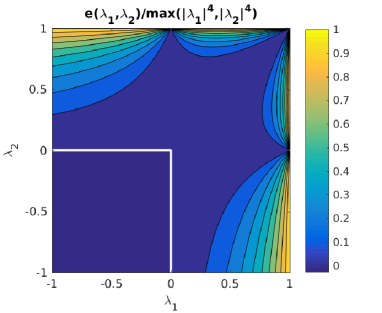
(a) Acceleration rate for AA^⋆(1) compared to theoretical contraction rate of Richardson iteration for contractive $2\times 2$ matrices.

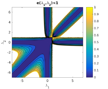
(b) The $(\lambda_{1},\lambda_{2})$-convergence plane for AA^⋆(1) applied to $2\times 2$ linear problems, characterizing which matrices guarantee AA^⋆ to define a uniform contraction.

Figure 1: Acceleration and convergence factor for the restarted AA^⋆(1).

Corollary 10 (AA^⋆(1) converges for non-contractive $\mathcal{FP}$).

Let the Assumption (C1)–(C4) be satisfied. Let $\mathbf{A}$ be positive definite with at most one eigenvalue among $\{\lambda_{1},\lambda_{2}\}$ larger than $1$ and none equal to $1$. Then AA^⋆(1) converges for the underlying non-contractive fixed-point iteration, cf. Assumption (C1).

Proof.

Due to symmetry, it is sufficient, to consider solely $(\lambda_{1},\lambda_{2})\in(\mathbb{R}_{+}\setminus\{1\})\times(0,1)$. For $\lambda_{1}<1$, the result follows immediately from Corollary 9. Let $\lambda_{1}>1$. It holds $e(1,\lambda_{2})=1$ for all $\lambda_{2}\in(0,1)$ and $\partial_{1}r(\lambda_{1},\lambda_{2})<0$ for all $(\lambda_{1},\lambda_{2})\in(1,\infty)\times(0,1)$. Thus, it follows directly that $r(\lambda_{1},\lambda_{2})<1$ for all $(\lambda_{1},\lambda_{2})\in(1,\infty)\times(0,1)$. ∎

7.3 Discussion

We make the following comments:

• The convergence result in Corollary 10 deals only with positive definite matrices. In Fig. 1b, eigenvalue pairs $(\lambda_{1},\lambda_{2})\in\mathbb{R}\times\mathbb{R}$ are displayed satisfying $r(\lambda_{1},\lambda_{2})<1$ and therefore guaranteeing AA^⋆(1) to converge. In particular, AA^⋆(1) converges also for matrices with two eigenvalues larger than 1 with relatively close distance to each other.

• In practice, we do not experience AA^⋆(1) or AA(1) to fail as long as Assumption (C4) is valid and $|\lambda_{1}|<1$ or $|\lambda_{2}|<1$. This observation extends also to arbitrarily large decompositions of $\mathbf{e}^{0}$ as long as at most one eigenvalue of $\mathbf{A}$ satisfies $|\lambda_{j}|>1$. Based on similar observations, we state the following claim: If $|\lambda_{j}|>1$ for exactly $m$ eigenvalues $\{\lambda_{j}\}_{j}$, then AA($m$) converges for arbitrary $\mathbf{e}^{0}$. We note that the worst case approach used to in order to prove Lemma 8 cannot be applied to prove the general claim. It can be verified numerically that in general the eigenvalues of the error propagation matrix (41) can be larger than 1 even if $\rho(\mathbf{A})<1$.

• From Fig. 1b, it follows, the closer the eigenvalues to $1$, the slower the convergence of AA^⋆(1). This is consistent with the interpretation of Anderson acceleration as secant method. The Richardson iteration does only damp slowly directions corresponding to eigenvalues close to 1. Hence, a directional derivative in these directions cannot be approximated well purely based on the iterations of fixed-point iterations. Quite contrary to directions corresponding to small or large eigenvalues relative to $1$.

• The theoretical convergence result has been obtained from a worst case analysis. Practical convergence rates might be lower than predicted, depending on the weights of the initial error.

• Convergence of AA($m$) is not guaranteed to be monotone, when applied for non-contractive fixed-point iterations.

8 Numerical results – Performance study

In this section, we will show three numerical examples, with increasing complexity, comparing the linearization schemes, presented in Section 4, coupled with Anderson acceleration. In particular, we confirm numerically the parabolic character of the nonlinear Biot equations, cf. Remark 3, the convergence result for the Fixed-Stress-L-scheme, cf. Theorem 7, as well as the acceleration and stabilization properties of the Anderson acceleration, cf. Section 7. All numerical results have been obtained using the software environment DUNE [36, 37, 38].

8.1 Test case I – Injection in a 2D homogeneous medium with Lipschitz continuous constitutive laws

We consider a two-dimensional, homogeneous, unsaturated porous medium $(-1,1)\times(0,1)$, in which a fluid is injected at the top, cf. Figure 2. Due to the symmetry of the problem, we consider only the right half $\Omega=(0,1)\times(0,1)$, discretized by $50\times 50$ regular quadrilaterals. As initial condition, we choose a constant displacement and pressure field with $\bm{u}(0)=\bm{0}$ and $p_{\mathrm{w}}(0)=p_{0}$, satisfying the stationary version of the continuous problem (1)–(3). In order to avoid inconsistent initial data, we ramp the injection at the top with inflow rate $q_{\mathrm{inflow}}(t)=q^{\star}\times\text{min}\,\{t^{2},1.0\}$ for given $q^{\star}\in\mathbb{R}$. Apart from the inflow at the top, we consider no flow at the remaining boundaries, no normal displacement at left, right and bottom boundary and no stress on the top. The boundary conditions are displayed in Figure 2.

\begin{overpic}[width=256.0748pt]{injection-geometry.eps} \put(67.0,28.0){$\bm{u}(0)=\bm{0}$} \put(64.75,23.0){$p_{\mathrm{w}}(0)=p_{0}$} \put(37.0,63.0){$\bm{q}_{\mathrm{w}}\cdot\bm{n}=q_{\mathrm{inflow}}$} \put(65.0,48.0){\footnotesize$\bm{q}_{\mathrm{w}}\cdot\bm{n}=0$,\ \ $\bm{\sigma}\bm{n}=\bm{0}$} \put(93.0,13.0){\rotatebox{90.0}{\footnotesize$\bm{q}_{\mathrm{w}}\cdot\bm{n}=0$,\ \ $\bm{u}\cdot\bm{n}=0$}} \put(50.0,13.0){\rotatebox{90.0}{\footnotesize$\bm{q}_{\mathrm{w}}\cdot\bm{n}=0$,\ \ $\bm{u}\cdot\bm{n}=0$}} \put(57.0,5.0){\footnotesize$\bm{q}_{\mathrm{w}}\cdot\bm{n}=0$,\ \ $\bm{u}\cdot\bm{n}=0$} \put(70.0,-3.0){\footnotesize$1\ [\mathrm{m}]$} \put(100.0,25.5){\footnotesize$1\ [\mathrm{m}]$} \put(51.0,45.0){\footnotesize$0.2\ [\mathrm{m}]$} \put(92.0,5.0){$\Omega$} \end{overpic}

Figure 2: Domain $\Omega$ and boundary conditions for test case I.

Physical and numerical parameters

For the constitutive laws, governing saturation and permeability, we use the van Genuchten-Mualem model [4], defining

$$s_{\mathrm{w}}(p_{\mathrm{w}}) =\left\{\begin{array}[]{l l}(1+(-{a_{\mathrm{vG}}}p_{\mathrm{w}})^{n_{\mathrm{vG}}})^{-\frac{{n_{\mathrm{vG}}}-1}{{n_{\mathrm{vG}}}}}&,p_{\mathrm{w}}\leq 0,\\ 1&,\text{else,}\end{array}\right. k_{\mathrm{w}}(s_{\mathrm{w}}) =\frac{k_{\mathrm{abs}}}{\mu_{w}}\,\sqrt{s_{\mathrm{w}}}\,\left(1-\left(1-s_{\mathrm{w}}^{\frac{{n_{\mathrm{vG}}}}{{n_{\mathrm{vG}}}-1}}\right)^{\frac{{n_{\mathrm{vG}}}-1}{{n_{\mathrm{vG}}}}}\right)^{2},\ s_{\mathrm{w}}\in[0,1],$$

where ${a_{\mathrm{vG}}}$ and ${n_{\mathrm{vG}}}$ are model parameters associated to the inverse of the air suction value and pore size distribution, respectively, $k_{\mathrm{abs}}$ is the intrinsic absolute permeability and $\mu_{w}$ is the dynamic fluid viscosity.

Parameter	Variable	Test case I	Test case II	Test case III
	[unit]	(Section 8.1)	(Section 8.2)	(Section 8.3)
Young’s modulus	$E$ [Pa]	3e1	3e1	1e6
Poisson’s ratio	$\nu$ [-]	0.2	0.2	0.3
Initial pressure	$p_{0}$ [Pa]	-7.78	$-$15.3	hydrostatic
Initial porosity	$\phi_{0}$ [-]	0.2	0.2	0.2
Inverse of air suction	${a_{\mathrm{vG}}}$ [Pa-1]	0.1844	0.627	$1\mathrm{e-}4$
Pore size distribution	${n_{\mathrm{vG}}}$ [-]	3.0	1.4	0.7-1
Abs. permeability	$k_{\mathrm{abs}}$ [m2]	3e$-$2	3e$-$2	$5\mathrm{e-}13$
Fluid viscosity	$\mu_{w}$ [Pa$\cdot$s]	1.0	1.0	$1\mathrm{e-}3$
Gravitational acc.	$\bm{g}$ [m/s2]	0.0	0.0	9.81
Biot coefficient	$\alpha$ [-]	0.1 $|$ 0.5 $|$ 1.0	0.1 $|$ 0.5 $|$ 1.0	1.0
Biot modulus	$N$ [Pa]	$\infty$	$\infty$	$\infty$
Maximal inflow rate	$q^{\star}$ [m2/s]	-1.25	-0.175	[-]
Final time	$T\ [\mathrm{s}]$	1.0	1.0	86400 ($=10\ [\mathrm{days}]$)
Time step size	$\tau\ [\mathrm{s}]$	1e$-$1	1e$-$1	3600 ($=1\ [\mathrm{hours}]$)
Absolute tolerance	$\varepsilon_{\mathrm{a}}$	1e$-$8	1e$-$8	$1\mathrm{e-}3$
Relative tolerance	$\varepsilon_{\mathrm{r}}$	1e$-$8	1e$-$8	$1\mathrm{e-}6$

Table 1: Parameters employed for test cases I and II. Top: Physical model parameters. Bottom: Numerical parameters.

Values chosen for model parameters and numerical parameters are displayed in Table 1. The parameters have been chosen such that the initial saturation is $s_{\mathrm{w,0}}=0.4$ in $\Omega$ and a region of full saturation ($s_{\mathrm{w}}=1$) is developed after seven time steps. Furthermore, the constitutive laws for saturation and permeability are Lipschitz continuous (with $L_{\mathrm{s}}=0.12$). We consider three different values for the Biot coefficient, controlling whether the Richards equation or the nonlinear coupling terms determine the character of the numerical difficulties. The simulation result for strong coupling ($\alpha=1.0$) at final time $t=1$ is illustrated exemplarily in Figure 3.

\begin{overpic}[width=455.3023pt]{injection-lipschitz-results.eps} \put(20.0,13.4){{\scriptsize$s_{\mathrm{w}}$}} \put(45.5,13.4){{\scriptsize$\sigma_{x}$ [Pa]}} \put(70.0,13.4){{\scriptsize$\tau_{xy}$ [Pa]}} \put(95.0,13.4){{\scriptsize$\sigma_{y}$ [Pa]}} \end{overpic}

Figure 3: Simulation results for test case I (Lipschitz continuous permeability): Saturation, normal stresses $\sigma_{x}$, $\sigma_{y}$ and shear stress $\tau_{xy}$ at time $t=1$.

Performance of linearization schemes

We consider the four linearization schemes introduced in Section 4, coupled with Anderson acceleration as post-processing. Abbreviations used in this section are introduced in Table 2.

Abbreviation	Explanation
Newton	Monolithic Newton’s method
FS-Newton	Fixed-Stress-Newton method
FS-MP	Fixed-Stress-Modified-Picard method
FSL	Fixed-Stress-L-scheme with $L=L_{\mathrm{s}}+\beta_{\mathrm{FS}}$
FSL/2	Fixed-Stress-L-scheme with $L=\tfrac{1}{2}(L_{\mathrm{s}}+\beta_{\mathrm{FS}})$
LIN-AA($m$)	Anderson accelerated linearization scheme LIN with $m+1$ reused iterations

Table 2: Abbreviations for methods (top) and additional stabilizations (bottom), where LIN is a variable.

We use the average number of iterations per time step as measure for performance, cf. Table 3. In particular, we disregard the use of CPU time as performance measure due to a not finely-tuned implementation. We just note, that a single iteration of a splitting method is significantly faster than a single monolithic Newton iteration.

First of all, all plain linearization schemes (AA(0)) succeed to converge for all three coupling strengths. This is consistent with Remark 3, demonstrating that the nonlinear Biot equations do not adopt the degeneracy of the Richards equation and remain parabolic in a fully saturated regime. Not surprisingly, the monolithic Newton method requires fewest iterations. So at first impression, it seems to be the preferred method. However, as stressed above, an advanced monolithic solver or an fixed-stress type iterative solver are required for efficient solution independent of the coupling strength, i.e., additional costs are hidden. On the other hand, the remaining linearization schemes allow separate simulators from the beginning. As the Fixed-Stress-L-scheme does not utilize an exact evaluation of derivatives, the Fixed-Stress-Newton method and the Fixed-Stress-Modified-Picard perform better for all three coupling strengths. Solely the performance of the Fixed-Stress-Newton method shows weak dependence on the coupling strength. The remaining methods show improved convergence behavior for increasing coupling strength, due to the decreasing numerical complexity of the problem itself following from Remark 3.

Linearization		Newton				FS-Newton				FS-MP				FSL				FSL/2
Biot coeff. $\alpha$		0.1	0.5	1.0		0.1	0.5	1.0		0.1	0.5	1.0		0.1	0.5	1.0		0.1	0.5	1.0
AA(0)		5.3	5.1	5.0		6.0	8.3	10.6		18.2	18.2	16.7		23.2	21.2	18.9		46.8	41.4	41.1
AA(1)		6.1	6.0	6.0		6.2	7.6	8.9		15.8	15.5	15.7		21.2	19.7	17.7		17.4	17.3	17.3
AA(3)		7.4	7.4	7.5		7.4	7.7	8.5		13.4	13.6	13.5		16.1	15.3	15.0		14.3	14.5	14.7
AA(5)		8.3	8.1	8.2		7.9	7.9	8.4		13.1	12.8	12.5		14.9	14.6	14.3		13.3	13.5	13.6
AA(10)		–	–	–		–	–	–		12.8	12.5	12.3		14.4	14.3	14.1		13.3	13.1	13.4

Table 3: Performance for test case I with different coupling strengths ($\alpha=0.1,\ 0.5,\ 1.0$). Average number of (nonlinear) iterations per time step for Newton’s method, the Fixed-Stress-Newton method, the Fixed-Stress-Modified-Picard method and the Fixed-Stress-L-scheme; both plain and coupled with Anderson acceleration for different depths ($m=1,\ 3,\ 5,\,10$). Minimal numbers per linearization type and Biot coefficient are in bold.

When applying Anderson acceleration, we observe that Anderson acceleration slows down the convergence of the monolithic Newton method, which is consistent with considerations in Section 6. In contrast, Anderson acceleration speeds up significantly the convergence of the Picard-type methods (Fixed-Stress-L-scheme and the variation FSL/2, and Fixed-Stress-Modified-Picard). Largest acceleration effect can be seen for largest considered depth. For the Fixed-Stress-Newton method, the effect of Anderson acceleration depends on the numerical character of the problem. This is due to the fact, that for weak coupling, the method is essentially identical with Newton’s method.

Regarding the Fixed-Stress-L-scheme, according to Theorem 7, optimally the diagonal stabilization parameter has to be chosen as small as possible. However, smaller values do not necessarily lead to faster convergence, as can be observed by comparing the plain Fixed-Stress-L-scheme and the plain FSL/2-scheme. Yet when utilizing Anderson acceleration, robustness with respect to the tuning parameter is increased, and eventually the FSL/2-scheme converges faster than the Fixed-Stress-L-scheme. In particular, it performs as good as the Fixed-Stress-Modified-Picard method.

All in all, the theory has been confirmed. The Fixed-Stress-L-scheme converges despite the simple linearization approach and Anderson acceleration is able to accelerate Picard-type schemes. Moreover, the latter has been shown to stabilize the Fixed-Stress-L-scheme, allowing to choose a small tuning parameter leading to improved convergence behavior. Considering the cost per iteration, despite some additional iterations, we finally recommend the use of the Fixed-Stress-Newton method with Anderson acceleration with low depth. It is cheap and allows separate simulators. For strongly coupled problems or in the absence of exact derivatives, the Fixed-Stress-L-scheme with small tuning parameter is an attractive alternative to the Fixed-Stress-Newton method.

8.2 Test case II – Injection in 2D homogeneous medium with Hölder continuous permeability

In the following, we reveal the limitations of the considered linearization schemes. Moreover, we demonstrate the stabilization property of Anderson acceleration, allowing non-convergent methods to converge. For this purpose, we repeat test case I with modified physical parameters. In particular, we choose the saturation to be Lipschitz continuous with same Lipschitz constant as in test case I. In contrast, the permeability is chosen to be only Hölder continuous. Hence, the derivative becomes unbounded in the transition between partial and full saturation, causing potential trouble for the Newton-type methods. Again, we choose the initial pressure and the maximal inflow rate such that $s_{\mathrm{w,0}}=0.4$ and a region of full saturation ($s_{\mathrm{w}}=1$) is developed after seven time steps. The simulation result for strong coupling at final time $t=1$ is illustrated in Figure 4.

\begin{overpic}[width=455.3023pt]{injection-hoelder-results.eps} \put(20.0,13.4){{\scriptsize$s_{\mathrm{w}}$}} \put(45.5,13.4){{\scriptsize$\sigma_{x}$ [Pa]}} \put(70.0,13.4){{\scriptsize$\tau_{xy}$ [Pa]}} \put(95.0,13.4){{\scriptsize$\sigma_{y}$ [Pa]}} \end{overpic}

Figure 4: Simulation results for test case II (Hölder continuous permeability): Saturation, normal stresses $\sigma_{x}$, $\sigma_{y}$ and shear stress $\tau_{xy}$ at time $t=1$.

As mentioned in Remark 5, due to lack of regularity for the permeability, each of the considered methods faces difficulties. For Newton-type methods (Newton, Fixed-Stress-Newton), the derivative of the permeability is evaluated, which might be unbounded. Effectively, for the Fixed-Stress-L-scheme, this also means that $L_{\mathrm{K}}\rightarrow\infty$ or in practice $L_{\mathrm{K}}$ becomes very large. Hence, by Theorem 7, the time step size has to be chosen sufficiently small or possibly $L$ has to be chosen larger to guarantee convergence. We note that for chosen initial saturation the permeability is significantly lower than for test case I. Consequently, the theoretical convergence rate for the plain Fixed-Stress-L-scheme (13)–(15) deteriorates. Due to round off errors stagnation is possible.

Performance of linearization schemes

Linearization		Newton				FS-Newton				FS-MP				FSL				FSL/2
Biot coeff. $\alpha$		0.1	0.5	1.0		0.1	0.5	1.0		0.1	0.5	1.0		0.1	0.5	1.0		0.1	0.5	1.0
AA(0)		$\bm{\nearrow}[8]$	8.5	8.1		$\bm{\nearrow}[9]$	13.2	19.1		$\bm{\rightarrow}[3]$	36.9	55.0		$\bm{\rightarrow}[9]$	126.9	134.9		$\bm{\rightarrow}[8]$	$\bm{\rightarrow}[9]$	$\bm{\rightarrow}[10]$
AA(1)		10.7	9.4	$\bm{\rightarrow}[8]$		11.0	11.8	14.6		45.2	34.2	33.8		133.6	84.0	83.2		$\bm{\rightarrow}[9]$	68.5	65.1
AA(3)		17.2	11.7	$\bm{\rightarrow}[8]$		15.6	12.1	13.0		30.5	26.9	28.1		68.3	54.3	56.9		48.4	37.9	35.5
AA(5)		24.8	13.9	$\bm{\rightarrow}[8]$		23.3	13.1	13.2		29.2	24.7	23.5		62.4	48.7	44.9		43.4	34.8	32.7
AA(10)		33.3	18.4	$\bm{\rightarrow}[8]$		43.0	14.7	13.8		29.8	23.5	23.5		52.6	42.6	42.5		39.3	31.8	29.2

Table 4: Performance for test case II with different coupling strengths ($\alpha=0.1,\ 0.5,\ 1.0$). Average number of (nonlinear) iterations per time step for Newton’s method, the Fixed-Stress-Newton method, the Fixed-Stress-Modified-Picard method and the Fixed-Stress-L-scheme; both plain and coupled with Anderson acceleration for different depths ($m=1,\ 3,\ 5,\,10$). Minimal numbers per linearization type and Biot coefficient are in bold. Failing linearization due to stagnation at time step $n$ is marked by $\bm{\rightarrow}[n]$. Failing linearization due to divergence at time step $n$ is marked by $\bm{\nearrow}[n]$.

The average number of iterations per time step is presented in Table 4. In contrast to test case I, not all plain linearization schemes (AA(0)) converge. For weak coupling, all Newton-like methods (Newton, Fixed-Stress-Newton) diverge with the Fixed-Stress-Newton method being slightly more robust due to added fixed-stress stabilization. The Fixed-Stress-L-scheme stagnates and shows to be slightly more robustness than the Newton-type methods. The Fixed-Stress-Modified-Picard method is least robust and stagnates already after two time steps. For strong coupling, all methods converge, which is consistent with Remark 3. If convergent, the schemes sorted by required number of iterations are the monolithic Newton method, the Fixed-Stress-Newton method, the Fixed-Stress-Modified-Picard and the Fixed-Stress-L-scheme, meeting our expectations.

By utilizing Anderson acceleration, convergence can be observed for all coupling strengths and all linearization schemes besides Newton’s method for $\alpha=1$. In particular, all previously failing schemes converge. This confirms the possible increase of robustness by Anderson acceleration, postulated in Section 7. Similar observations as before are made for the splitting schemes under Anderson acceleration. All in all, the theory has been confirmed.

As before, for increasing depth, the performance of Newton’s method deteriorates. For strong coupling stagnation is observed. For weak coupling, for several time steps practical stagnation is observed with eventual convergence after a very large number of iterations. This is consistent with the fact that Anderson acceleration can also lead to divergence for increasing depth [30]. Hence, Anderson acceleration has to be applied carefully for the monolithic Newton method.

Motivated by test case I, we apply the Fixed-Stress-L-scheme with a decreased tuning parameter. For this test case, the plain FSL/2-scheme fails for all coupling strengths. As the FSL/2-scheme is a priori less robust as the Fixed-Stress-L-scheme, this has been expected. Utilizing Anderson acceleration, the FSL/2-scheme eventually converges. In particular, convergence is always faster than for the corresponding Fixed-Stress-L-scheme. This again demonstrates the ability of the Anderson acceleration to increase robustness and to relax assumptions for practical convergence.

According to the theory for the Fixed-Stress-L-scheme, a larger tuning parameter or a lower time step size could enable convergence, e.g., for $\alpha=0.1$, AA(0). However, we do not consider those strategies here, as they lead to worse convergence rates and utilizing Anderson acceleration should be anyhow preferred.

Concerning the best splitting method, we again recommend the use of the Fixed-Stress-Newton method combined with Anderson acceleration with low depth. It is cheap, robust and allows separate simulators.

8.3 Test case III – Unsteady seepage flow through a 2D homogeneous levee

We consider unsteady seepage flow through a simple, two-dimensional, homogeneous levee, enforced by a flood. The levee consists of a lower and upper part (lower $5\ [\mathrm{m}]$ and upper $10\ [\mathrm{m}]$, respectively), cf. Figure 5. Initially, the water table lies at the interface between lower and upper part. The initial fluid pressure is a hydrostatic pressure with $p=0$ at the water table. The reference configuration, defined by the domain, is initially already consolidated under the influence of gravity. As $\bm{u}$ is the deviation of the reference configuration, effectively, no gravity is applied in the mechanics equation, but only in the flow equation.

\begin{overpic}[width=341.43306pt]{levee-geometry.eps} \put(78.0,32.0){\small Seepage face} \put(17.5,28.0){\small$t>0$} \put(39.0,18.3){\small$t=0$} \put(90.5,18.5){\small$t\geq 0$} \put(101.0,23.0){\small$\bm{g}$} \put(11.0,21.7){\small$h(t)$} \put(-3.0,23.5){\rotatebox{90.0}{\small$10\ [\mathrm{m}]$}} \put(-3.0,10.5){\rotatebox{90.0}{\small$5\ [\mathrm{m}]$}} \put(14.0,-2.8){\small$10\ [\mathrm{m}]$} \put(33.0,-2.8){\small$10\ [\mathrm{m}]$} \put(48.0,-2.8){\small$5\ [\mathrm{m}]$} \put(61.0,-2.8){\small$10\ [\mathrm{m}]$} \put(80.0,-2.8){\small$10\ [\mathrm{m}]$} \end{overpic}

Figure 5: Domain, boundary and initial conditions for test case III.

Over time, on the left hand side of the levee, the water table rises with constant speed for four days and remains constant for the next six days, defining $h(t)=2t\ [\mathrm{m/days}]$, $t\leq 4\ [\mathrm{days}]$ and $h(t)=8\ [\mathrm{m}]$, $t\geq 4\ [\mathrm{days}]$. Below $h(t)$ on the left, a hydrostatic pressure boundary condition is applied. On the right side, we apply approximate seepage face boundary conditions, based on the previous time step; i.e., given a fully saturated cell at the previous time step, a pressure boundary condition $p=0$ is applied on corresponding boundary for the next time step, otherwise a no-flow boundary condition is applied for the volumetric flux. On the remaining boundary, no-flow boundary conditions are applied for all time. For the mechanics, no displacement in normal direction is assumed on the boundary of the lower part of the levee. On the boundary of the upper part and the interface, zero effective stress is applied. The boundary conditions are visualized in Figure 5.

Physical and numerical parameters

The domain is discretized by a regular, unstructured, simplicial mesh with approximately 67,000 elements and 201,000 nodes. Compared to the previous test cases, we employ more realistic material parameters. Values chosen for model parameters and numerical parameters are displayed in Table 1. We note, the resulting permeability is only Hölder continuous. The saturation history and deformation at four times is displayed in Figure 6. We observe steep saturation gradients during the flooding. Furthermore, both consolidation and swelling can be observed. All in all, the levee is pushed to the right.

\begin{overpic}[width=341.43306pt]{levee-saturation-history-2.eps} \put(2.0,35.0){$0\ [\mathrm{days}]$} \put(47.0,35.0){$2.5\ [\mathrm{days}]$} \put(2.0,14.0){$5\ [\mathrm{days}]$} \put(47.0,14.0){$10\ [\mathrm{days}]$} \put(95.0,32.0){$s_{\mathrm{w}}$} \end{overpic}

Figure 6: Simulation result for test case III. Saturation for the deformed material at time $t=0\ [\mathrm{days}],2.5\ [\mathrm{days}],5\ [\mathrm{days}],10\ [\mathrm{days}]$. Direction and intensity of deformation also indicated by arrows.

Performance of linearization schemes

We consider the same linearization schemes as in the previous test cases, all but FSL, i.e., the Fixed-Stress-L-scheme with $L=L_{\mathrm{s}}+\beta_{\mathrm{FS}}$. Based on previous observations, we expect FSL/2 coupled with Anderson acceleration to be more efficient than FSL. The average number of iterations per time step is presented in Table 5. First of all, we observe that all plain linearization schemes fail in the same phase of the simulation (after around 50 time steps). The reason for that lies mainly in the steep saturation gradients. As before, Anderson acceleration can yield remedy. However, for this test case, the simple combination of Newton’s method and Anderson acceleration does not converge for any considered depth. Newton’s method combined with Anderson acceleration is still not convergent for AA(1). For increasing depth the robustness decreases again, which is consistent with observations from the previous test cases. For the remaining linearization schemes convergence can be obtained. In particular, the Fixed-Stress-Newton method combined with AA(1) converges with the least amount of iterations. The Picard-type methods are slower, but show again more robustness with respect to increasing depth, whereas the Fixed-Stress-Newton method diverges eventually for $m=10$. Here, the Picard type methods require at least depth $m=3$ for successful convergence. After all, we conclude that the diagonal stabilization is essential for the success of the linearization schemes. The stabilization is added via both the fixed-stress splitting scheme and the L-scheme. Consequently, we expect also the monolithic Newton method to be convergent when adding sufficient diagonal stabilization.

Linearization		Newton		FS-Newton		FS-MP		FSL/2
AA(0)		$\bm{\nearrow}[56]$		$\bm{\rightarrow}[57]$		$\bm{\rightarrow}[48]$		$\bm{\rightarrow}[48]$
AA(1)		$\bm{\rightarrow}\textbf{[165]}$		10.2		$\bm{\rightarrow}[86]$		$\bm{\rightarrow}[73]$
AA(3)		$\bm{\rightarrow}[90]$		11.4		18.1		33.2
AA(5)		$\bm{\rightarrow}[87]$		10.6		16.9		30.2
AA(10)		$\bm{\rightarrow}[87]$		$\bm{\rightarrow}[87]$		16.0		28.3

Table 5: Performance for test case III. Average number of (nonlinear) iterations per time step for Newton’s method, the Fixed-Stress-Newton method, the Fixed-Stress-Modified-Picard method and the Fixed-Stress-L-scheme; both plain and coupled with Anderson acceleration for different depths ($m=1,\ 3,\ 5,\,10$). Minimal numbers per linearization type are in bold. Failing linearization due to stagnation at time step $n$ is marked by $\bm{\rightarrow}[n]$. Failing linearization due to divergence at time step $n$ is marked by $\bm{\nearrow}[n]$.

9 Concluding remarks

In this paper, we have proposed three different linearization schemes for nonlinear poromechanics of unsaturated materials. All schemes incorporate the fixed-stress splitting scheme and allow the efficient and robust decoupling of mechanics and flow equations. In particular, the simplest scheme, the Fixed-Stress-L-scheme, employs solely constant diagonal stabilization. It has been derived as L-scheme linearization of the Biot equations reduced to a pure pressure formulation. Under mild, physical assumptions, also needed for the mathematical model to be valid, it has been rigorously shown to be a contraction. This also has been verified numerically. Exploiting the derivation of the Fixed-Stress-L-scheme allows modifications including first order Taylor approximations. In this way, we have introduced the Fixed-Stress-Modified-Picard and the Fixed-Stress-Newton method.

The derivation of the Fixed-Stress-L-scheme provides two particular side products. First, it reveals the close relation of the L-scheme and the fixed-stress splitting scheme. Second, the nonlinear Biot equations can be shown to be parabolic in the pressure variable. This holds in particular in the fully saturated regime unlike for the Richards equation.

The theoretical convergence rate of the Fixed-Stress-L-scheme might deteriorate for unfavorable situations, leading to slow convergence or even stagnation in practice. Similarly, the Fixed-Stress-Modified-Picard and Fixed-Stress-Newton methods are prone to diverge for Hölder continuous nonlinearities. In order to accelerate or retain convergence, we apply Anderson acceleration, which is a post-processing, maintaining the decoupled character of the underlying splitting methods. The general increase of robustness and acceleration of convergence via the Anderson acceleration has been justified theoretically considering a special linear case. To our knowledge, this is the first theoretical indication of this kind, considering non-contractive fixed-point iterations.

In practice, Anderson acceleration has shown to be very effective for the considered Picard-type methods, confirming the theoretical considerations. After all, we recommend the combination of the Fixed-Stress-Newton method and the Anderson acceleration, being very robust even for Hölder continuous nonlinearities. In case analytical derivatives are not available, we recommend the combination of the Fixed-Stress-L-scheme with a decreased tuning parameter and Anderson acceleration. Without Anderson acceleration, convergence might not be guaranteed. Including it, does not only retain but it also significantly accelerates convergence. This is interesting, as the optimal tuning parameter is not necessarily known a priori and can be more safely approached under the use of Anderson acceleration.

As outlook, with focus on large scale applications, the performance of the linearization schemes should be analyzed under the use of parallel, iterative solvers; in particular, as due to added stabilization, the arising linear systems are expected to be better conditioned than for the monolithic Newton method. Additionally, Anderson acceleration should be further studied in the context of possibly non-contractive fixed point iterations. Examples are (i) the linearization of degenerate problems including Hölder continuities, which are known to be difficult to solve [23], and (ii) numerical schemes employing a tuning parameter. Based on the numerical results in this paper, the approach seems very promising.

Appendix A Convergence proof of abstract L-scheme

We present the proof of Lemma 1 showing convergence of the L-scheme (27) as linearization for Eq. (26). The proof is essentially the same as given by [22], but now written for an algebraic problem.

Proof of Lemma 1.

Let $\mathbf{e}_{\mathbf{p}}^{i}=\mathbf{p}^{i}-\mathbf{p}$. Then taking the difference of Eq. (27) and (26) yields

$$\mathbf{L}_{\mathrm{pp}}\left(\mathbf{e}_{\mathbf{p}}^{i}-\mathbf{e}_{\mathbf{p}}^{i-1}\right)+\left(\mathbf{b}(\mathbf{p}^{i-1})-\mathbf{b}(\mathbf{p})\right)+\tau\mathbf{D}\mathbf{K}(\mathbf{p}^{i-1})\mathbf{D}^{\top}\mathbf{e}_{\mathbf{p}}^{i}+\tau\mathbf{D}\left(\mathbf{K}(\mathbf{p}^{i-1})-\mathbf{K}(\mathbf{p})\right)\left(\mathbf{f}_{\mathrm{q}}+\mathbf{D}^{\top}\mathbf{p}\right) =0.$$

Multiplying with $\mathbf{e}_{\mathbf{p}}^{i}$ and applying elementary algebraic manipulations, yields

$$\frac{L}{2}\|\mathbf{e}_{\mathbf{p}}^{i}\|_{\mathbf{M}_{\mathrm{pp}}}^{2}+\frac{L}{2}\|\mathbf{e}_{\mathbf{p}}^{i}-\mathbf{e}_{\mathbf{p}}^{i-1}\|_{\mathbf{M}_{\mathrm{pp}}}^{2}-\frac{L}{2}\|\mathbf{e}_{\mathbf{p}}^{i-1}\|_{\mathbf{M}_{\mathrm{pp}}}^{2}$$ (42)

$$\quad+\langle\mathbf{b}(\mathbf{p}^{i-1})-\mathbf{b}(\mathbf{p}),\mathbf{e}_{\mathbf{p}}^{i-1}\rangle$$ (43)

$$\quad+\langle\mathbf{b}(\mathbf{p}^{i-1})-\mathbf{b}(\mathbf{p}),\mathbf{e}_{\mathbf{p}}^{i}-\mathbf{e}_{\mathbf{p}}^{i-1}\rangle$$ (44)

$$\quad+\tau\langle\mathbf{K}(\mathbf{p}^{i-1})\mathbf{D}^{\top}\mathbf{e}_{\mathbf{p}}^{i},\mathbf{D}^{\top}\mathbf{e}_{\mathbf{p}}^{i}\rangle$$ (45)

$$\quad+\tau\langle\left(\mathbf{K}(\mathbf{p}^{i-1})-\mathbf{K}(\mathbf{p})\right)\left(\mathbf{f}_{\mathrm{q}}+\mathbf{D}^{\top}\mathbf{p}\right),\mathbf{D}^{\top}\mathbf{e}_{\mathbf{p}}^{i}\rangle=0.$$ (46)

By employing (L1), we obtain for the term (43)

$$\langle\mathbf{b}(\mathbf{p}^{i-1})-\mathbf{b}(\mathbf{p}),\mathbf{e}_{\mathbf{p}}^{i-1}\rangle\geq\frac{1}{L_{\mathrm{b}}}\left\|\mathbf{b}(\mathbf{p}^{i-1})-\mathbf{b}(\mathbf{p})\right\|_{\mathbf{M}_{\mathrm{pp}}^{-1}}^{2}.$$ (47)

By employing the Cauchy-Schwarz inequality and Young’s inequality, we obtain for the term (44)

$$\langle\mathbf{b}(\mathbf{p}^{i-1})-\mathbf{b}(\mathbf{p}),\mathbf{e}_{\mathbf{p}}^{i}-\mathbf{e}_{\mathbf{p}}^{i-1}\rangle\geq-\frac{1}{2L}\left\|\mathbf{b}(\mathbf{p}^{i-1})-\mathbf{b}(\mathbf{p})\right\|_{\mathbf{M}_{\mathrm{pp}}^{-1}}^{2}-\frac{L}{2}\left\|\mathbf{e}_{\mathbf{p}}^{i}-\mathbf{e}_{\mathbf{p}}^{i-1}\right\|_{\mathbf{M}_{\mathrm{pp}}}^{2}.$$ (48)

By employing Assumption (L2), we obtain for the term (45)

$$\langle\mathbf{K}(\mathbf{p}^{i-1})\mathbf{D}^{\top}\mathbf{e}_{\mathbf{p}}^{i},\mathbf{D}^{\top}\mathbf{e}_{\mathbf{p}}^{i}\rangle\geq k_{\mathrm{m}}\|\mathbf{D}^{\top}\mathbf{e}_{\mathbf{p}}^{i}\|_{\mathbf{M}_{\mathrm{qq}}^{-1}}^{2}.$$ (49)

By employing Cauchy-Schwarz, Young’s inequality, Assumption (L2)–(L3), we obtain for the term (46)

$$\langle\left(\mathbf{K}(\mathbf{p}^{i-1})-\mathbf{K}(\mathbf{p})\right)\left(\mathbf{f}_{\mathrm{q}}+\mathbf{D}^{\top}\mathbf{p}\right),\mathbf{D}^{\top}\mathbf{e}_{\mathbf{p}}^{i}\rangle \geq-\frac{1}{2k_{\mathrm{m}}}\|{\mathbf{M}_{\mathrm{qq}}^{-1}}(\mathbf{f}_{\mathrm{q}}+\mathbf{D}^{\top}\mathbf{p})\|_{\infty}^{2}\|(\mathbf{K}(\mathbf{p}^{i-1})-\mathbf{K}(\mathbf{p}))\mathbf{M}_{\mathrm{qq}}\|_{\mathbf{M}_{\mathrm{qq}},\infty}^{2}-\frac{k_{\mathrm{m}}}{2}\|\mathbf{D}^{\top}\mathbf{e}_{\mathbf{p}}^{i}\|_{\mathbf{M}_{\mathrm{qq}}^{-1}}^{2}$$

$$\geq-\frac{1}{2k_{\mathrm{m}}}q_{\infty}^{2}L_{\mathrm{K}}^{2}\|\mathbf{b}(\mathbf{p}^{i-1})-\mathbf{b}(\mathbf{p})\|_{\mathbf{M}_{\mathrm{qq}}^{-1}}^{2}-\frac{k_{\mathrm{m}}}{2}\|\mathbf{D}^{\top}\mathbf{e}_{\mathbf{p}}^{i}\|_{\mathbf{M}_{\mathrm{qq}}^{-1}}^{2}.$$ (50)

Inserting Eq. (47)–(50) into Eq. (42)–(46), yields

$$\left(\frac{1}{L_{\mathrm{b}}}-\frac{1}{2L}-\tau\frac{q_{\infty}^{2}L_{\mathrm{K}}^{2}}{2k_{\mathrm{m}}}\right)\|\mathbf{b}(\mathbf{p}^{i-1})-\mathbf{b}(\mathbf{p})\|_{\mathbf{M}_{\mathrm{pp}}^{-1}}^{2}+\frac{L}{2}\|\mathbf{e}_{\mathbf{p}}^{i}\|_{\mathbf{M}_{\mathrm{pp}}}^{2}+\tau\frac{k_{\mathrm{m}}}{2}\|\mathbf{D}^{\top}\mathbf{e}_{\mathbf{p}}^{i}\|_{\mathbf{M}_{\mathrm{qq}}^{-1}}^{2}\leq\frac{L}{2}\|\mathbf{e}_{\mathbf{p}}^{i-1}\|_{\mathbf{M}_{\mathrm{pp}}}^{2}.$$ (51)

Assuming $\frac{1}{L_{\mathrm{b}}}-\frac{1}{2L}-\tau\frac{q_{\infty}^{2}L_{\mathrm{K}}^{2}}{2k_{\mathrm{m}}}\geq 0$ and applying an algebraic Poincaré inequality, yields the final result. ∎

References

- [1] M. Biot, “General theory of three-dimensional consolidation,” Journal of applied physics, vol. 12, no. 2, pp. 155–164, 1941.
- [2] O. Coussy, Poromechanics. Wiley, 2004.
- [3] J. Kim, H. A. Tchelepi, and R. Juanes, “Rigorous Coupling of Geomechanics and Multiphase Flow with Strong Capillarity,” Society of Petroleum Engineers, 2013.
- [4] van Genuchten, “A closed-form equation for predicting the hydraulic conductivity of unsaturated soils,” Soil Science Society of America Journal, vol. 44(5), pp. 892–898, 1980.
- [5] A. Settari and F. Mourits, “A coupled reservoir and geomechanical simulation system,” Society of Petroleum Engineers, vol. 3, pp. 219 – 226, 1998.
- [6] J. A. White and R. I. Borja, “Block-preconditioned Newton–Krylov solvers for fully coupled flow and geomechanics,” Computational Geosciences, vol. 15, no. 4, p. 647, 2011.
- [7] J. Kim, H. A. Tchelepi, and R. Juanes, “Stability, Accuracy, and Efficiency of Sequential Methods for Coupled Flow and Geomechanics,” Society of Petroleum Engineers, 2011.
- [8] A. Mikelić and M. F. Wheeler, “Convergence of iterative coupling for coupled flow and geomechanics,” Computational Geosciences, vol. 17, no. 3, pp. 455–461, 2013.
- [9] J. W. Both, M. Borregales, J. M. Nordbotten, K. Kumar, and F. A. Radu, “Robust fixed stress splitting for Biot’s equations in heterogeneous media,” Applied Mathematics Letters, vol. 68, pp. 101 – 108, 2017.
- [10] M. Bause, F. A. Radu, and U. Köcher, “Space–time finite element approximation of the biot poroelasticity system with iterative coupling,” Computer Methods in Applied Mechanics and Engineering, vol. 320, pp. 745 – 768, 2017.
- [11] M. Borregales, K. Kumar, F. A. Radu, C. Rodrigo, and F. José Gaspar, “A parallel-in-time fixed-stress splitting method for Biot’s consolidation model,” ArXiv e-prints, Feb. 2018.
- [12] S. Dana, B. Ganis, and M. F. Wheeler, “A multiscale fixed stress split iterative scheme for coupled flow and poromechanics in deep subsurface reservoirs,” Journal of Computational Physics, vol. 352, pp. 1 – 22, 2018.
- [13] N. Castelletto, J. A. White, and H. A. Tchelepi, “Accuracy and convergence properties of the fixed-stress iterative solution of two-way coupled poromechanics,” International Journal for Numerical and Analytical Methods in Geomechanics, vol. 39, no. 14, pp. 1593–1618, 2015.
- [14] N. Castelletto, J. A. White, and M. Ferronato, “Scalable algorithms for three-field mixed finite element coupled poromechanics,” Journal of Computational Physics, vol. 327, pp. 894 – 918, 2016.
- [15] J. A. White, N. Castelletto, and H. A. Tchelepi, “Block-partitioned solvers for coupled poromechanics: A unified framework,” Computer Methods in Applied Mechanics and Engineering, vol. 303, pp. 55 – 74, 2016.
- [16] J. H. Adler, F. J. Gaspar, X. Hu, C. Rodrigo, and L. T. Zikatanov, “Robust Block Preconditioners for Biot’s Model,” arXiv:1705.08842 [math.NA], 2017.
- [17] F. J. Gaspar and C. Rodrigo, “On the fixed-stress split scheme as smoother in multigrid methods for coupling flow and geomechanics,” Computer Methods in Applied Mechanics and Engineering, vol. 326, pp. 526 – 540, 2017.
- [18] M. Slodicka, “A Robust and Efficient Linearization Scheme for Doubly Nonlinear and Degenerate Parabolic Problems Arising in Flow in Porous Media,” SIAM Journal on Scientific Computing, vol. 23, no. 5, pp. 1593–1614, 2002.
- [19] I. S. Pop, F. A. Radu, and P. Knabner, “Mixed finite elements for the Richards’ equation: linearization procedure,” Journal of Computational and Applied Mathematics, vol. 168, no. 1, pp. 365 – 373, 2004.
- [20] F. A. Radu, J. M. Nordbotten, I. S. Pop, and K. Kumar, “A robust linearization scheme for finite volume based discretizations for simulation of two-phase flow in porous media,” Journal of Computational and Applied Mathematics, vol. 289, pp. 134 – 141, 2015.
- [21] F. A. Radu, K. Kumar, J. M. Nordbotten, and I. S. Pop, “A robust, mass conservative scheme for two-phase flow in porous media including Hölder continuous nonlinearities,” IMA Journal of Numerical Analysis, p. drx032, 2017.
- [22] F. List and F. A. Radu, “A study on iterative methods for solving Richards’ equation,” Computational Geosciences, vol. 20, no. 2, pp. 341–353, 2016.
- [23] J. W. Both, K. Kumar, J. M. Nordbotten, I. Sorin Pop, and F. A. Radu, “Linear iterative schemes for doubly degenerate parabolic equations,” ArXiv e-prints, 2018.
- [24] D. Seus, K. Mitra, I. S. Pop, F. A. Radu, and C. Rohde, “A linear domain decomposition method for partially saturated flow in porous media,” Computer Methods in Applied Mechanics and Engineering, vol. 333, pp. 331 – 355, 2018.
- [25] M. Borregales, F. A. Radu, K. Kumar, and J. M. Nordbotten, “Robust iterative schemes for non-linear poromechanics,” arXiv:1702.00328, 2017.
- [26] M. A. Celia, E. T. Bouloutas, and R. L. Zarba, “A general mass-conservative numerical solution for the unsaturated flow equation,” Water Resources Research, vol. 26, no. 7, pp. 1483–1496, 1990.
- [27] D. G. Anderson, “Iterative Procedures for Nonlinear Integral Equations,” Journal of the Association for Computing Machinery, vol. 12, no. 4, pp. 547–560, 1965.
- [28] P. Lott, H. Walker, C. Woodward, and U. Yang, “An accelerated Picard method for nonlinear systems related to variably saturated flow,” Advances in Water Resources, vol. 38, pp. 92 – 101, 2012.
- [29] H. Fang and Y. Saad, “Two classes of multisecant methods for nonlinear acceleration,” Numerical Linear Algebra with Applications, vol. 16, no. 3, pp. 197–221, 2009.
- [30] H. F. Walker and P. Ni, “Anderson Acceleration for Fixed-Point Iterations,” SIAM J. Numer. Anal., vol. 49, no. 4, pp. 1715–1735, 2011.
- [31] A. Toth and C. T. Kelley, “Convergence Analysis for Anderson Acceleration,” SIAM Journal on Numerical Analysis, vol. 53, no. 2, pp. 805–819, 2015.
- [32] C. Paniconi and M. Putti, “A comparison of Picard and Newton iteration in the numerical solution of multidimensional variably saturated flow problems,” Water Resources Research, vol. 30, no. 12, pp. 3357–3374, 1994.
- [33] C. Rodrigo, X. Hu, P. Ohm, J. H. Adler, F. J. Gaspar, and L. Zikatanov, “New stabilized discretizations for poroelasticity and the Stokes’ equations,” ArXiv e-prints, June 2017.
- [34] J. W. Both and U. Köcher, “Numerical investigation on the fixed-stress splitting scheme for Biot’s equations: Optimality of the tuning parameter,” ArXiv e-prints, 2018.
- [35] R. Showalter and N. Su, “Partially saturated flow in a poroelastic medium,” Discrete and Continuous Dynamical Systems - Series B, vol. 1, no. 4, pp. 403–420, 2001.
- [36] P. Bastian, M. Blatt, A. Dedner, C. Engwer, R. Klöfkorn, M. Ohlberger, and O. Sander, “A generic grid interface for parallel and adaptive scientific computing. Part I: abstract framework,” Computing, vol. 82, no. 2, pp. 103–119, 2008.
- [37] P. Bastian, M. Blatt, A. Dedner, C. Engwer, R. Klöfkorn, R. Kornhuber, M. Ohlberger, and O. Sander, “A generic grid interface for parallel and adaptive scientific computing. Part II: implementation and tests in DUNE,” Computing, vol. 82, no. 2, pp. 121–138, 2008.
- [38] M. Blatt, A. Burchardt, A. Dedner, C. Engwer, J. Fahlke, B. Flemisch, C. Gersbacher, C. Gräser, F. Gruber, C. Grüninger, D. Kempf, R. Klöfkorn, T. Malkmus, S. Müthing, M. Nolte, M. Piatkowski, and O. Sander, “The Distributed and Unified Numerics Environment, Version 2.4,” Archive of Numerical Software, vol. 4, no. 100, pp. 13–29, 2016.