A new class of curves of rational B-spline type

Résumé

Une nouvelle classe de paramétrisation rationnelle a été développée et on l’a utilisée pour générer une nouvelle famille de fonctions B-splines rationnelles $\displaystyle{{\left({{{}^{\alpha}}{\bf G}_{i}^{k}}\right)}_{i=0}^{k}}$ qui dépend d’un indice $\alpha\in{\left({-\infty}\,,\,{0}\right)}\cup{\left({1}\,,\,{+\infty}\right)}$. Cette famille de fonctions vérifie entre autres, les propriétés de positivité, de partition de l’unité et, pour un dégré $k$ donné, constitue une véritable base d’approximation de fonctions continues. On perd cependant la régularité optimale classique liée à la multiplicité des nœuds, ce que l’on récupère dans le cas asymptotique, lorsque $\alpha\to\infty$.

Les courbes de type B-splines associées vérifient les propriétés traditionnelles notamment celle d’enveloppe convexe et l’on voit apparaître une certaine ”symétrie conjuguée” liée à $\alpha$.

Le cas des vecteurs nœuds ouverts sans nœud intérieur conduit à une nouvelle famille de courbes de Bézier rationnelles qui fera, séparément, l’objet d’une analyse approfondie.

Abstract

A new class of rational parametrization has been developed and it was used to generate a new family of rational functions B-splines $\displaystyle{{\left({{{}^{\alpha}}{\bf G}_{i}^{k}}\right)}_{i=0}^{k}}$ which depends on an index $\alpha\in(-\infty,0)\cup(1,+\infty)$. This family of functions verifies, among other things, the properties of positivity, of partition of the unit and, for a given degree $k$, constitutes a true basis approximation of continuous functions. We loose, however, the regularity classical optimal linked to the multiplicity of nodes, which we recover in the asymptotic case, when $\alpha\longrightarrow\infty$. The associated B-splines curves verify the traditional properties particularly that of a convex hull and we see a certain ”conjugated symmetry” related to $\alpha$. The case of open knot vectors without an inner node leads to a new family of rational Bezier curves that will be separately, object of in-depth analysis.

Mots clés : Vecteur nœud, Fonctions B-splines rationnelles, Relation de Cox de-Boor, Algorithme de de-Boor, Graphisme Informatique.

Keywords : Knot vector, Rational B-splines functions , Cox- de Boor recursion, de-Boor Algorithm, Computer Graphics.

1 Introduction

A standard B-spline curve $G$ of degree $k\in{\bf I\!\!\!N}^{*}$ in ${\bf I\!\!R}^{d}$ with $d\in{\bf I\!\!\!N}^{*}$, $1\leq d\leq 3$ is defined by a polynomial basis ${\left({{}{\bf G}_{i}^{k}}\right)}_{i=0}^{n}$ on a parametrization space $[a\,,\,b]$ subdivided by a knot vector $U={\left({t_{i}}\right)}_{i=0}^{m}$ with $m=n+k+1$. The basis ${\left({{}{\bf G}_{i}^{k}}\right)}_{i=0}^{n}$ is given by the recurrence relation of Cox/de Boor [4] as follows:

$$\begin{array}[]{rcl}{}{\bf G}_{i}^{0}(x)&=&\left\{{\begin{array}[]{ll}1&\textrm{if }t_{i}\leq x<t_{i+1}\textrm{ for }i=0,\ldots,m-1\\ 0&\textrm{otherwise }\end{array}}\right.\\ {}{\bf G}_{i}^{k}(x)&=&w_{i}^{k}(x){}{\bf G}_{i}^{k-1}(x)+{\left(1-w_{i+1}^{k}(x)\right)}{}{\bf G}_{i+1}^{k-1}(x)\\ w_{i}^{k}(x)&=&\left\{{\begin{array}[]{ll}\displaystyle{\frac{x-t_{i}}{t_{i+k}-t_{i}}}&\textrm{if }t_{i}\leq x<t_{i+k}\textrm{ for }i=0,\ldots,n\\ 0&\textrm{otherwise }\end{array}}\right.\\ \end{array}$$ (1)

If $\displaystyle{{\left({d_{i}}\right)}_{i=0}^{n}}$ are the control polygon vertices of $G$, $d_{i}\in{\bf I\!\!R}^{d}$ for all $i$ then

$$G(x)=\displaystyle{\sum_{i=0}^{n}d_{i}\,{}{\bf G}_{i}^{k}(x)}\,,\,\forall x\in[a\,,\,b]$$

Likewise we have the rational B-spline basis ${\left({R_{i}}\right)}_{i=0}^{n}$ of degree $k\in{\bf I\!\!\!N}^{*}$ associated to the knot vector $U$ and the weight vector $W={\left({\omega_{i}}\right)}_{i=0}^{n}$ which can be defined by

$$R_{i}(x)=\displaystyle{\frac{\omega_{i}{}{\bf G}_{i}^{n}(x)}{\displaystyle{\sum_{j=0}^{n}\omega_{j}{}{\bf G}_{j}^{n}(x)}}}$$

where $\omega_{i}>0,\,\forall i=0,\ldots,n$.

We can then define the rational B-spline curves replacing the polynomial basis by the rational basis [4],[6].

One has to notice that $\displaystyle{w_{i}^{k}(x)=\varphi{\left({x}\,,\,{t_{i}}\,,\,{t_{i+k}}\right)}}$ where $\varphi$ is a real function defined on ${\bf I\!\!R}^{3}$ satisfying the following properties:

1. $\displaystyle{\varphi{\left({x}\,,\,{a}\,,\,{b}\right)}\in[0\,,\,1)}$ for all ${\left({x}\,,\,{a}\,,\,{b}\right)}\in{\bf I\!\!R}^{3}$

2. For all $a,b\in{\bf I\!\!R}$ such that $a<b$ the function $\displaystyle{x\in{\bf I\!\!R}\mapsto\varphi{\left({x}\,,\,{a}\,,\,{b}\right)}}$ is continuous, strictly increasing on $[a\,,\,b)$ and we have:

   • $\displaystyle{\varphi{\left({x}\,,\,{a}\,,\,{b}\right)}=0}$ for all $x\notin(a\,,\,b)$

   • $\displaystyle{\lim_{x\to b^{-}}\varphi{\left({x}\,,\,{a}\,,\,{b}\right)}=1}$

The aim of this work is to maintain these properties while imposing that for all $a,b\in{\bf I\!\!R}$ such that $a<b$, the function $\displaystyle{x\in{\bf I\!\!R}\mapsto\varphi{\left({x}\,,\,{a}\,,\,{b}\right)}}$ is homographic in order to build a natural B-spline basis composed of rational functions.

2 A class of rational parametrization

2.1 Definition

The targeted class of parametrization is based on the following lemma which gives the foundation of a new class of curves of rational B-spline type.

Lemma 2.1

Let $a,\,b\in{\bf I\!\!R}$ verifying $a<b$. There exists a family ${\cal H}\left(\left[{a}\,,\,{b}\right]\right)$ of homographic functions $f$ strictly increasing on $[a\,,\,b]$ such that $f(a)=0$ and $f(b)=1$.

More precisely, for all $f\in{\cal H}\left(\left[{a}\,,\,{b}\right]\right)$ there exists a unique
$\alpha\in(-\infty\,,\,0)\cup(1\,,\,\infty)$ such that

$$f(x)=\displaystyle{\frac{\alpha(x-a)}{x+(\alpha-1)b-\alpha a}},\quad\forall x\in[a\,,\,b]$$

Proof
( Existence ) Since $f$ is homographic with $f(a)=0$ there exists $\alpha\neq 0$ and $c\in{\bf I\!\!R}\backslash\{-a,\,-b\}$ such that for all $x\in[a\,,\,b]$ we get: $\displaystyle{f(x)=\frac{\alpha(x-a)}{x+c}}$. As $f(b)=1$ then $\displaystyle{1=\frac{\alpha(b-a)}{b+c}}$. This leads to $c=(\alpha-1)b-\alpha a$. Using the fact that $c\notin\{-a,\,-b\}$ then we have $\alpha\notin\{0,\,1\}$. The strict increase of $f$ yields $\alpha(\alpha-1)>0$, therefore $\alpha\in(-\infty\,,\,0)\cup(1\,,\,\infty)$.

We then write

$${\cal H}\left(\left[{a}\,,\,{b}\right]\right)=\left\{\displaystyle{f_{\alpha}}|\,\displaystyle{f_{\alpha}(x)}=\displaystyle{\frac{\alpha(x-a)}{x+(\alpha-1)b-\alpha a}},\,\alpha\in(-\infty\,,\,0)\cup(1\,,\,\infty),\,x\in[a\,,\,b]\right\}$$

( Uniqueness )

Let $\alpha,\,\beta\in(-\infty\,,\,0)\cup(1\,,\,\infty)$ and $f_{\alpha},\,f_{\beta}\in{\cal H}\left(\left[{a}\,,\,{b}\right]\right)$ corresponding

$$\begin{array}[]{lcl}f_{\alpha}=f_{\beta}&\,\Leftrightarrow&f_{\alpha}(x)=f_{\beta}(x)\quad\forall x\in[a\,,\,b]\\ &\,\Rightarrow&\displaystyle{\frac{\alpha(x-a)}{x+(\alpha-1)b-\alpha a}}=\displaystyle{\frac{\beta(x-a)}{x+(\beta-1)b-\beta a}}\quad\forall x\in[a\,,\,b]\\ &\,\Rightarrow&\displaystyle{(\alpha-\beta)(x-b)}=0\quad\forall x\in[a\,,\,b]\\ &\,\Rightarrow&\displaystyle{(\alpha-\beta)(x-b)}=0\quad\forall x\in[a\,,\,b[\\ &\,\Rightarrow&\displaystyle{\alpha=\beta}\end{array}$$

Remark 2.1

Let $x\in[a\,,\,b]$ and $\alpha\in(-\infty\,,\,0)\cup(1\,,\,\infty)$.
One has $D=x+(\alpha-1)b-\alpha a\neq 0$.

Indeed, Observing that $D=x-b+\alpha(b-a)=x-a+(\alpha-1)(b-a)$, we have $(\alpha-1)(b-a)\leq D\leq\alpha(b-a)$. One can then deduce that

$$\left\{\begin{array}[]{ll}0<\alpha(\alpha-1)(b-a)\leq\alpha D\leq\alpha^{2}(b-a)&\textrm{ if }\alpha>1\\ 0<\alpha^{2}(b-a)\leq\alpha D\leq\alpha(\alpha-1)(b-a)&\textrm{ if }\alpha<0\end{array}\right.$$

Thus $D\neq 0\,\forall x\in[a\,,\,b]$.

Remark 2.2

Let $\alpha\in(-\infty\,,\,0)\cup(1\,,\,\infty)$ and $a<b$.
$f_{\alpha}\in{\cal H}\left(\left[{a}\,,\,{b}\right]\right)$ is continuous and strictly increasing on $[a\,,\,b]$ with $f_{\alpha}([a\,,\,b])=[0\,,\,1]$.

Moreover for $\lambda\in[0\,,\,1]$ and for $x=a+\lambda(b-a)\in[a\,,\,b]$ we have

$$f_{\alpha}(x)=\displaystyle{\frac{\lambda\alpha}{\lambda+\alpha-1}\in[0\,,\,1]}$$

We thus obtain the classical case as an asymptotic situation; indeed:

$${\lim_{\left|{\alpha}\right|\to\infty}f_{\alpha}(x)=\lambda=\frac{x-a}{b-a}}$$

Remark 2.3

Let $\alpha\in(-\infty\,,\,0)\cup(1\,,\,\infty)$ and $a<b$.
Let $f_{\alpha},f_{1-\alpha}\in{\cal H}\left(\left[{a}\,,\,{b}\right]\right)$. For all $x\in[a\,,\,b]$, we have:

$$\begin{array}[]{rcl}\displaystyle{f_{\alpha}(a+b-x)}&=&\displaystyle{1-f_{1-\alpha}(x)}\\ \displaystyle{f_{\alpha}(x)}&=&\displaystyle{1-f_{1-\alpha}(a+b-x)}\\ \end{array}$$

Indeed, we observe that $x\in[a\,,\,b]$ is equivalent to $a+b-x\in[a\,,\,b]$ and

$$\begin{array}[]{rcl}\displaystyle{f_{\alpha}(a+b-x)}&=&\displaystyle{\frac{\alpha{\left(b-x\right)}}{-x+\alpha b+{\left(1-\alpha\right)}a}}\\ &=&\displaystyle{-\frac{\alpha{\left(b-x\right)}}{x-\alpha b-{\left(1-\alpha\right)}a}}\\ \displaystyle{1-f_{1-\alpha}(x)}&=&\displaystyle{1-\frac{{\left(1-\alpha\right)}{\left(x-a\right)}}{x+{\left[{\left(1-\alpha\right)}-1\right]}b-{\left(1-\alpha\right)}a}}\\ &=&\displaystyle{1-\frac{{\left(1-\alpha\right)}{\left(x-a\right)}}{x-\alpha b-{\left(1-\alpha\right)}a}}\\ &=&\displaystyle{-\frac{\alpha{\left(b-x\right)}}{x-\alpha b-{\left(1-\alpha\right)}a}}\\ &=&\displaystyle{f_{\alpha}(a+b-x)}\\ \end{array}$$

We obtain the second relation by a simple change of variables.

From now on, we say that $\alpha$ and $1-\alpha$ are conjugated.

Definition 2.1

Let $\alpha\in(-\infty\,,\,0)\cup(1\,,\,\infty)$. A parametrization of index $\alpha$ is any real function $\varphi_{\alpha}$ defined for all ${\left({x}\,,\,{a}\,,\,{b}\right)}\in{\bf I\!\!R}^{3}$ by

$$\varphi_{\alpha}{\left({x}\,,\,{a}\,,\,{b}\right)}=\left\{\begin{array}[]{ll}f_{\alpha}(x)&\textrm{if }a\leq x<b\textrm{ with }f_{\alpha}\in{\cal H}\left(\left[{a}\,,\,{b}\right]\right)\\ 0&\textrm{otherwise}\end{array}\right.$$

2.2 Properties of the parametrization

Proposition 2.1

Let $\alpha\in(-\infty\,,\,0)\cup(1\,,\,\infty)$ and $\varphi_{\alpha}$ the associated parametrization. Let $T$ be an affine and bijective function of ${\bf I\!\!R}$. The following properties hold: For all ${\left({x}\,,\,{a}\,,\,{b}\right)}\in{\bf I\!\!R}^{3}$

1. $\displaystyle{0\leq\varphi_{\alpha}{\left({x}\,,\,{a}\,,\,{b}\right)}<1}$

2. If $T$ is strictly increasing then

   $${\varphi_{\alpha}{\left({T(x)}\,,\,{T(a)}\,,\,{T(b)}\right)}=\varphi_{\alpha}{\left({x}\,,\,{a}\,,\,{b}\right)}}$$

3. If $T$ is strictly decreasing then

   $${\varphi_{\alpha}{\left({T(x)}\,,\,{T(b)}\,,\,{T(a)}\right)}=1-\varphi_{1-\alpha}{\left({x}\,,\,{a}\,,\,{b}\right)}}$$

Proof
Let $T$ be an affine and bijective function of ${\bf I\!\!R}$. There exists ${\left({\lambda}\,,\,{\delta}\right)}\in{\bf I\!\!R}^{*}\times{\bf I\!\!R}$ such that, for all $x\in{\bf I\!\!R}$, we have $\displaystyle{T(x)=\lambda x+\delta}$.

Let ${\left({x}\,,\,{a}\,,\,{b}\right)}\in{\bf I\!\!R}^{3}$

1. If $T$ is strictly increasing and $a<x<b$ then $T(a)<T(x)<T(b)$

   $$\begin{array}[]{rcl}\displaystyle{\varphi_{\alpha}{\left({T(x)}\,,\,{T(a)}\,,\,{T(b)}\right)}}&=&\displaystyle{f_{\alpha}{(T(x))}\textrm{ with }f_{\alpha}\in{\cal H}\left(\left[{T(a)}\,,\,{T(b)}\right]\right)}\\ &=&\displaystyle{\frac{\alpha{\left[T(x)-T(a)\right]}}{T(x)+(\alpha-1)T(b)-\alpha T(a)}}\\ &=&\displaystyle{\frac{\alpha{\left[(\lambda x+\delta)-(\lambda a+\delta)\right]}}{(\lambda x+\delta)+(\alpha-1)(\lambda b+\delta)-\alpha(\lambda a+\delta)}}\\ &=&\displaystyle{\frac{\alpha\lambda{\left[x-a\right]}}{\lambda{\left[x+(\alpha-1)b-\alpha a\right]}}}\\ &=&\displaystyle{\frac{\alpha{\left[x-a\right]}}{x+(\alpha-1)b-\alpha a}}\\ &=&\displaystyle{g_{\alpha}{(x)}\textrm{ with }g_{\alpha}\in{\cal H}\left(\left[{a}\,,\,{b}\right]\right)}\\ &=&\displaystyle{\varphi_{\alpha}{\left({x}\,,\,{a}\,,\,{b}\right)}}\\ \end{array}$$

2. If $T$ is strictly decreasing and $a<x<b$ then $T(b)<T(x)<T(a)$

   $$\begin{array}[]{rcl}\displaystyle{\varphi_{\alpha}{\left({T(x)}\,,\,{T(b)}\,,\,{T(a)}\right)}}&=&\displaystyle{f_{\alpha}{(T(x))}\textrm{ with }f_{\alpha}\in{\cal H}\left(\left[{T(b)}\,,\,{T(a)}\right]\right)}\\ &=&\displaystyle{\frac{\alpha{\left[T(x)-T(b)\right]}}{T(x)+(\alpha-1)T(a)-\alpha T(b)}}\\ &=&\displaystyle{\frac{\alpha{\left[(\lambda x+\delta)-(\lambda b+\delta)\right]}}{(\lambda x+\delta)+(\alpha-1)(\lambda a+\delta)-\alpha(\lambda b+\delta)}}\\ &=&\displaystyle{\frac{\alpha\lambda{\left[x-b\right]}}{\lambda{\left[x+(\alpha-1)a-\alpha b\right]}}}\\ &=&\displaystyle{\frac{\alpha{\left[x-b\right]}}{x+(\alpha-1)a-\alpha b}}\\ &=&\displaystyle{\frac{\alpha{\left[x-b\right]}}{x-\alpha b-(1-\alpha)a}}\\ &=&\displaystyle{1-\frac{(1-\alpha){\left[x-a\right]}}{x-\alpha b-(1-\alpha)a}}\\ &=&\displaystyle{1-g_{1-\alpha}{(x)}\textrm{ with }g_{1-\alpha}\in{\cal H}\left(\left[{a}\,,\,{b}\right]\right)}\\ &=&\displaystyle{1-\varphi_{1-\alpha}{\left({x}\,,\,{a}\,,\,{b}\right)}}\\ \end{array}$$

Corollary 2.1

Let $\alpha\in(-\infty\,,\,0)\cup(1\,,\,\infty)$ and $\varphi_{\alpha}$ be the associated parametrization. Let $a,b\in{\bf I\!\!R}$ such that $a<b$. Let $a<t_{1}<t_{2}<b$. For all $x\in[a\,,\,b]$, we have

$${\varphi_{\alpha}{\left({a+b-x}\,,\,{t_{1}}\,,\,{t_{2}}\right)}=1-\varphi_{1-\alpha}{\left({x}\,,\,{a+b-t_{2}}\,,\,{a+b-t_{1}}\right)}}$$

Proof
We apply proposition 2.1 by taking $\displaystyle{T(x)=a+b-x}$ on ${\bf I\!\!R}$. We observe that $T$ is strictly decreasing and verifies $T\circ T(x)=x$ for all $x\in{\bf I\!\!R}$. This gives the result.

Remark 2.4

Let $a,b\in{\bf I\!\!R}$ such that $a<b$. The function

$${x\in{\bf I\!\!R}\mapsto\varphi_{\alpha}{\left({x}\,,\,{a}\,,\,{b}\right)}}$$

is continuous on ${\bf I\!\!R}\backslash\{b\}$ and we have:

$$\begin{array}[]{rcl}\displaystyle{\varphi_{\alpha}{\left({a}\,,\,{a}\,,\,{b}\right)}}&=&0\\ \displaystyle{\lim_{x\to b^{-}}\varphi_{\alpha}{\left({x}\,,\,{a}\,,\,{b}\right)}}&=&1\\ \displaystyle{\lim_{x\to b^{+}}\varphi_{\alpha}{\left({x}\,,\,{a}\,,\,{b}\right)}}&=&0\\ \end{array}$$ (2)

On the other hand, this function is of class ${\cal C}^{\infty}$ on $(-\infty\,,\,a)\cup(a\,,\,b)\cup(b\,,\,\infty)$ and one has:

$$\begin{array}[]{rcl}\displaystyle{\lim_{x\to a^{-}}\frac{d\varphi_{\alpha}}{dx}{\left({x}\,,\,{a}\,,\,{b}\right)}}&=&0\\ \displaystyle{\lim_{x\to a^{+}}\frac{d\varphi_{\alpha}}{dx}{\left({x}\,,\,{a}\,,\,{b}\right)}}&=&\displaystyle{\frac{\alpha}{\left(\alpha-1\right)\left(b-a\right)}}\\ \displaystyle{\lim_{x\to b^{-}}\frac{d\varphi_{\alpha}}{dx}{\left({x}\,,\,{a}\,,\,{b}\right)}}&=&\displaystyle{\frac{\alpha-1}{\alpha\left(b-a\right)}}\\ \displaystyle{\lim_{x\to b^{+}}\frac{d\varphi_{\alpha}}{dx}{\left({x}\,,\,{a}\,,\,{b}\right)}}&=&0\\ \end{array}$$ (3)

Illustration 2.1

The figures 1 and 2 illustrate $\displaystyle{\varphi_{\alpha}{\left({x}\,,\,{0}\,,\,{1}\right)}}$ for $\displaystyle{x\in(-1\,,\,2)}$ with values of $\alpha$ conjugated respectively.

We observe that on the subinterval $\displaystyle{(0\,,\,1)}$ which is the interior of its support, the function is convex for $\displaystyle{\alpha<0}$ and concave for $\displaystyle{\alpha>1}$.

The figure 3 which illustrates $\displaystyle{\varphi_{\alpha}{\left({x}\,,\,{1}\,,\,{3}\right)}}$ for $\displaystyle{x\in(0\,,\,6)}$ confirms the previous observations and lets suspect the symmetrical role that the conjugated $\alpha$ are to play. It also shows that the effect of $\alpha$ is crucial in the neighborhood of $0$ and of $1$.

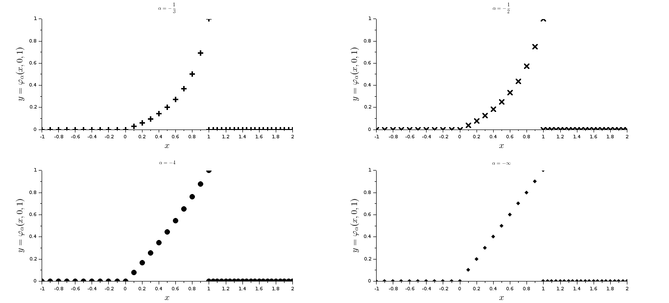
Figure 1: The curves of $\displaystyle{\varphi_{\alpha}}$ for $\alpha\in\{-\frac{1}{3},-\frac{1}{2},-4,\infty\}$

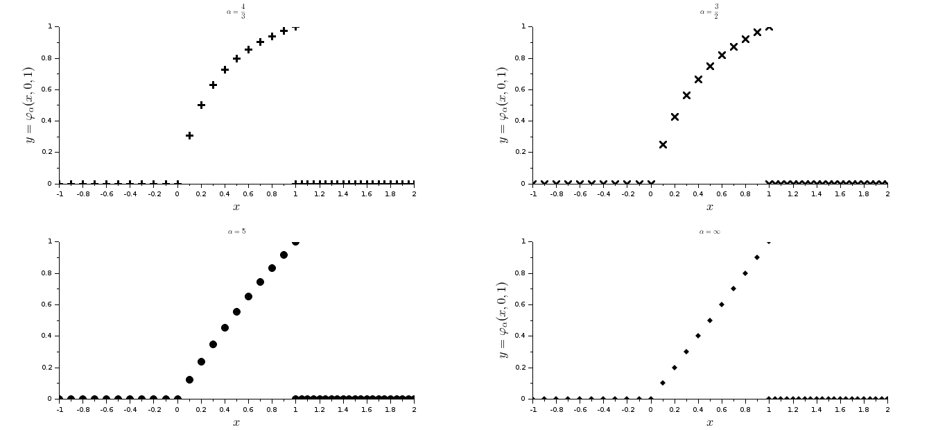
Figure 2: The curves $\displaystyle{\varphi_{\alpha}}$ for $\alpha\in\{\frac{4}{3},\frac{3}{2},5,\infty\}$

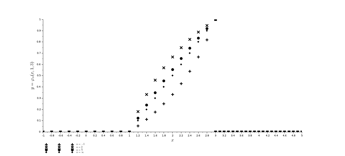
Figure 3: Comparaison of $\displaystyle{\varphi_{\alpha}}$ for conjugated $\alpha$ and large $\alpha$

3 New class of rational B-splines basis

3.1 Definitions

The B-splines curves are part of the family of curves obtained by concatenation of several generated pieces of curves using a family of basic functions of parametrization space $[a\,,\,b]$ subdivised by a knot vector $U$ and a set of points ${\left({d_{i}}\right)}_{i=0}^{n}$ of ${\bf I\!\!R}^{d}$ called control polygon.

The nature of chosen knot vector may strongly influence the properties of B-spline basis generated as well as the resulting curve. We must very quickly specify this object.

We follow the definitions of the book of D. F. Rogers entitled ”An Introduction to NURBS with historical perspective” [4].

Definition 3.1

Let $a,b\in{\bf I\!\!R}$ such that $a<b$. A knot vector in $[a,b]$ is any increasing sequence $U={\left({t_{i}}\right)}_{i=0}^{m}$ in $[a\,,\,b]$.

The knot vectors fall into two categories: the open knot vectors and periodic knot vectors. Each category is divided in two variants: uniform and non-uniform.

Definition 3.2

Let $a,b\in{\bf I\!\!R}$ such that $a<b$ and $m,k\in{\bf I\!\!\!N}^{*}$ such that $m>2k$. We consider the knot vector $U={\left({t_{i}}\right)}_{i=0}^{m}$ such that $t_{k}=a$ and $t_{m-k}=b$.

1. End nodes:

   The nodes $t_{0},t_{1},\ldots,t_{k}$ and the nodes $t_{m-k},t_{m-k+1},\ldots,t_{m}$ are called end nodes.

   The nodes $t_{k+1},t_{k+2},\ldots,t_{m-k-1}$ are called interior nodes.

2. Open knot vector:

   The knot vector is said to be open if its end nodes coincide; we then have $t_{0}=t_{1}=\ldots=t_{k}=a$ and $t_{m-k}=t_{m-k+1}=\ldots=t_{m}=b$.

   Otherwise $U$ is said to be periodic.

3. Uniform knot vector :

   $U$ is uniform if its interior nodes are equidistant; that is, there exists $h>0$ such that $t_{i+1}-t_{i}=h$ for all $k\leq i\leq m-k-1$.

   Otherwise $U$ is non-uniform.

4. Multiple node (multiplicity of a node) :

   Let $p\in{\bf I\!\!\!N}^{*}$ and $t_{i}$ be a node of $U$. We say that $t_{i}$ is a node of multiplicity $p$ if there exists a unique $j\in[0,\ldots,m-1]\cap{\bf I\!\!\!N}$ such that the subsequence $U_{i}={\left({t_{j+l}}\right)}_{l=0}^{p-1}$ with $j\leq i\leq j+p-1$ is constant.

   If $p>1$, we say that $t_{i}$ is multiple node.

5. Breakpoints:

   The set ${\left({u_{i}}\right)}_{i=0}^{r}$ of distinct nodes of $U={\left({t_{i}}\right)}_{i=0}^{m}$ constitutes the breakpoints. We have $u_{0}=t_{0}<u_{1}<\ldots<u_{r}=t_{m}$ and there exists a unique sequence of nonnegative integers $p={\left({p_{i}}\right)}_{i=0}^{r}$ such that for all $i=0,\ldots,r$, $u_{i}$ is of multiplicity $p_{i}$.

   We shall remark that $\displaystyle{\sum_{i=0}^{r}p_{i}=m+1}$. On the other hand, these nodes define the different segments of studied curves and the interior breakpoints define the transition between its segments.

6. Symmetrical knot vector:

   $U={\left({t_{i}}\right)}_{i=0}^{m}$ is a symmetrical knot vector if for all $i=0,\ldots,m$, $t_{m-i}=t_{0}+t_{m}-t_{i}$.

Definition 3.3

Let $a,b\in{\bf I\!\!R}$ such that $a<b$ and $m,n,k\in{\bf I\!\!\!N}^{*}$ such that $n\geq k$ and $m=n+k+1$. Let $\alpha\in(-\infty\,,\,0)\cup(1\,,\,\infty)$ and $\displaystyle{\varphi_{\alpha}}$ the parametrization of index $\alpha$. Let $U={\left({t_{i}}\right)}_{i=0}^{m}$ be a knot vector of the interval $[a\,,\,b]$.

A B-spline basis of index $\alpha$ and of degree $k$ on the node vector $U$ is the real functions ${\left({{{}^{\alpha}}{\bf G}_{i}^{k}}\right)}_{i=0}^{n}$ defined by the recurrence relation:

$$\begin{array}[]{rcl}\displaystyle{{{}^{\alpha}}{\bf G}_{i}^{0}(x)}&=&\left\{{\begin{array}[]{ll}1&\textrm{if }t_{i}\leq x<t_{i+1}\textrm{ for }i=0,\ldots,m-1\\ 0&\textrm{otherwise }\end{array}}\right.\\ \displaystyle{{{}^{\alpha}}{\bf G}_{i}^{k}(x)}&=&\displaystyle{w_{i}^{k}(x){{}^{\alpha}}{\bf G}_{i}^{k-1}(x)+{\left(1-w_{i+1}^{k}(x)\right)}{{}^{\alpha}}{\bf G}_{i+1}^{k-1}(x)}\\ \displaystyle{w_{i}^{k}(x)}&=&\displaystyle{\varphi_{\alpha}{\left({x}\,,\,{t_{i}}\,,\,{t_{i+k}}\right)}}\\ \end{array}$$ (4)

This relation is said to be of Cox/de Boor.

Definition 3.4

Let $a,b\in{\bf I\!\!R}$ such that $a<b$. Let $m,n,k\in{\bf I\!\!\!N}^{*}$ such that $n>k$ and $m=n+k+1$. Let $\alpha\in(-\infty\,,\,0)\cup(1\,,\,\infty)$. Let $U={\left({t_{i}}\right)}_{i=0}^{m}$ be a knot vector of interval $[a\,,\,b]$. Let $d\in{\bf I\!\!\!N}^{*}$ such that $d\leq 3$, and $\displaystyle{\Pi={\left({d_{i}}\right)}_{i=0}^{n}\subset{\bf I\!\!R}^{d}}$.

Let ${\left({{{}^{\alpha}}{\bf G}_{i}^{k}}\right)}_{i=0}^{n}$ be the B-spline basis of index $\alpha$, of degree $k$ and of knot vector $U$.

A B-spline curve of index $\alpha$, with knot vector $U$ and control points $\displaystyle{{\left({d_{i}}\right)}_{i=0}^{n}}$ is the ${\bf I\!\!R}^{d}$ valued function $G_{\alpha}$ defined by:

$${x\in{\left[{t_{0}}\,,\,{t_{m}}\right]}\mapsto G_{\alpha}(x)=\sum_{i=0}^{n}d_{i}{{}^{\alpha}}{\bf G}_{i}^{k}(x)}$$

$\Pi$ is called control polygon of the curve $G_{\alpha}$.

3.2 Fundamental properties of the next class of basis

Proposition 3.1

Let $m,k,n\in{\bf I\!\!\!N}^{*}$ such that $n\geq k$ and $m=n+k+1$. Let $\displaystyle{U={\left({t_{i}}\right)}_{i=0}^{m}}$ be a knot vector and $\alpha\in(-\infty\,,\,0)\cup(1\,,\,\infty)$.

The rational B-spline basis of index $\alpha$ with knot vector $U$ and of degree $k$, ${\left({{{}^{\alpha}}{\bf G}_{i}^{k}}\right)}_{i=0}^{n}$, verifies the following properties:

1. Local support property:

   For all $x\notin(t_{i}\,,\,t_{i+k+1})$, ${{}^{\alpha}}{\bf G}_{i}^{k}(x)=0$

2. Positivity property:

   For all $i=0,\ldots,n$ and $x\in(t_{i}\,,\,t_{i+k+1})$, ${{}^{\alpha}}{\bf G}_{i}^{k}(x)>0$

3. Unit partition property:

   For all $j$ such that $t_{j}<t_{j+1}$, for all $x\in[t_{j}\,,\,t_{j+1})$, we have

   $${\sum_{i=0}^{n}{{}^{\alpha}}{\bf G}_{i}^{k}(x)=\sum_{i=j-k}^{j}{{}^{\alpha}}{\bf G}_{i}^{k}(x)=1}$$

4. Symmetry property:

   If $U$ is a symmetrical knot vector then for all $x\in[t_{0}\,,\,t_{m}]$ and $i=0,\ldots,n$ we have

   $${{}^{\alpha}}{\bf G}_{i}^{k}(t_{0}+t_{m}-x)={{}^{1-\alpha}}{\bf G}_{n-i}^{k}(x)$$

Proof
Let $\alpha\in(-\infty\,,\,0)\cup(1\,,\,\infty)$ and $\displaystyle{\varphi_{\alpha}}$ be the parametrization of index $\alpha$.

We will proceed by recurrence on $k$.

1. (Local support and Positivity: )

   • For $k=0$, we have by definition: for all $i=0,\ldots,m-1$

     $${{}^{\alpha}}{\bf G}_{i}^{0}(x)=\left\{\begin{array}[]{ll}1&\textrm{if }t_{i}\leq x<t_{i+1}\textrm{ for }i=0,\ldots,m-1\\ 0&\textrm{otherwise }\end{array}\right.$$

     hence we have

     $$\begin{array}[]{ll}\displaystyle{{{}^{\alpha}}{\bf G}_{i}^{k}(x)}=0&\textrm{ if }\displaystyle{x\notin(t_{i}\,,\,t_{i+k+1})}\\ \displaystyle{{{}^{\alpha}}{\bf G}_{i}^{k}(x)}>0&\textrm{ if }\displaystyle{x\in(t_{i}\,,\,t_{i+k+1})\neq\emptyset}\\ \end{array}$$

   • Let $k>0$ and assume that for all $0\leq j<k$ we have

     $$\begin{array}[]{ll}\displaystyle{{{}^{\alpha}}{\bf G}_{i}^{j}(x)}=0&\textrm{ if }\displaystyle{x\notin(t_{i}\,,\,t_{i+j+1})}\\ \displaystyle{{{}^{\alpha}}{\bf G}_{i}^{j}(x)}>0&\textrm{ if }\displaystyle{x\in(t_{i}\,,\,t_{i+j+1})\neq\emptyset}\\ \end{array}$$

     By definition we have

     $${{{}^{\alpha}}{\bf G}_{i}^{k}(x)=w_{i}^{k}(x){{}^{\alpha}}{\bf G}_{i}^{k-1}(x)+{\left(1-w_{i+1}^{k}(x)\right)}{{}^{\alpha}}{\bf G}_{i+1}^{k-1}(x)}$$

     with

     $$\begin{array}[]{l}\left\{\begin{array}[]{ll}\displaystyle{{{}^{\alpha}}{\bf G}_{i}^{k-1}(x)}=0&\textrm{ if }\displaystyle{x\notin(t_{i}\,,\,t_{i+k})}\\ \displaystyle{{{}^{\alpha}}{\bf G}_{i}^{k-1}(x)}>0&\textrm{ if }\displaystyle{x\in(t_{i}\,,\,t_{i+k})\neq\emptyset}\\ \end{array}\right.\\ \textrm{ and }\\ \left\{\begin{array}[]{ll}\displaystyle{{{}^{\alpha}}{\bf G}_{i+1}^{k-1}(x)}=0&\textrm{ if }\displaystyle{x\notin(t_{i+1}\,,\,t_{i+k+1})}\\ \displaystyle{{{}^{\alpha}}{\bf G}_{i+1}^{k-1}(x)}>0&\textrm{ if }\displaystyle{x\in(t_{i+1}\,,\,t_{i+k+1})\neq\emptyset}\\ \end{array}\right.\\ \end{array}$$

     • Let $\displaystyle{x\notin(t_{i}\,,\,t_{i+k+1})=(t_{i}\,,\,t_{i+k})\cup(t_{i+1}\,,\,t_{i+k+1})}$. Then we have $\displaystyle{x\notin(t_{i}\,,\,t_{i+k})}$ and $\displaystyle{x\notin(t_{i+1}\,,\,t_{i+k+1})}$ which gives $\displaystyle{{{}^{\alpha}}{\bf G}_{i}^{k-1}(x)}=0$, $\displaystyle{{{}^{\alpha}}{\bf G}_{i+1}^{k-1}(x)}=0$ and $\displaystyle{{{}^{\alpha}}{\bf G}_{i}^{k}(x)}=0$

     • Let $\displaystyle{x\in(t_{i}\,,\,t_{i+k+1})=(t_{i}\,,\,t_{i+k})\cup(t_{i+1}\,,\,t_{i+k+1})\neq\emptyset}$. Then we have $\displaystyle{x\in(t_{i}\,,\,t_{i+k})\neq\emptyset}$ or $\displaystyle{x\in(t_{i+1}\,,\,t_{i+k+1})\neq\emptyset}$.

       If $\displaystyle{x\in(t_{i}\,,\,t_{i+k})\neq\emptyset}$ then one has $\displaystyle{{{}^{\alpha}}{\bf G}_{i}^{k-1}(x)}>0$ and $\displaystyle{{{}^{\alpha}}{\bf G}_{i+1}^{k-1}(x)}\geq 0$. But from proposition 2.1 we have

       $$\left\{\begin{array}[]{l}\displaystyle{w_{i}^{k}(x)=\varphi_{\alpha}{\left({x}\,,\,{t_{i}}\,,\,{t_{i+k}}\right)}\in(0\,,\,1)}\\ \displaystyle{w_{i+1}^{k}(x)=\varphi_{\alpha}{\left({x}\,,\,{t_{i+1}}\,,\,{t_{i+k+1}}\right)}\geq 0}\\ \end{array}\right.$$

       We conclude that

       $${{{}^{\alpha}}{\bf G}_{i}^{k}(x)\geq w_{i}^{k}(x){{}^{\alpha}}{\bf G}_{i}^{k-1}(x)>0}$$

       Similarly if $\displaystyle{x\in(t_{i+1}\,,\,t_{i+k+1})\neq\emptyset}$ then $\displaystyle{{{}^{\alpha}}{\bf G}_{i}^{k-1}(x)}\geq 0$ and $\displaystyle{{{}^{\alpha}}{\bf G}_{i+1}^{k-1}(x)}>0$. By using once more proposition 2.1 we have

       $$\left\{\begin{array}[]{l}\displaystyle{w_{i}^{k}(x)=\varphi_{\alpha}{\left({x}\,,\,{t_{i}}\,,\,{t_{i+k}}\right)}\geq 0}\\ \displaystyle{w_{i+1}^{k}(x)=\varphi_{\alpha}{\left({x}\,,\,{t_{i+1}}\,,\,{t_{i+k+1}}\right)}\in(0\,,\,1)}\\ \end{array}\right.$$

       We then conclude that

       $${{{}^{\alpha}}{\bf G}_{i}^{k}(x)\geq{\left(1-w_{i+1}^{k}(x)\right)}{{}^{\alpha}}{\bf G}_{i+1}^{k-1}(x)>0}$$

       Hence $\displaystyle{{{}^{\alpha}}{\bf G}_{i}^{k}(x)>0}$ if $\displaystyle{x\in(t_{i}\,,\,t_{i+k+1})}$

2. (Unit partition)

   Let $m,k,n\in{\bf I\!\!\!N}^{*}$ such that $n>k$ and $m=n+k+1$.

   • Let $j$ such that $t_{j}<t_{j+1}$. Let $i=0,\ldots,n$.

     $$[t_{i}\,,\,t_{i+k+1})\cap[t_{j}\,,\,t_{j+1})\neq\emptyset\,\Leftrightarrow\,j-k\leq i\leq j$$

   • Let $x\in[t_{j}\,,\,t_{j+1})$ and $i=0,\ldots,n$.

     $${{}^{\alpha}}{\bf G}_{i}^{k}(x)\neq 0\,\Leftrightarrow\,j-k\leq i\leq j$$

     Thus we have $\displaystyle{\sum_{i=0}^{n}{{}^{\alpha}}{\bf G}_{i}^{k}(x)=\sum_{i=j-k}^{j}{{}^{\alpha}}{\bf G}_{i}^{k}(x)}$.

     As $\displaystyle{{{}^{\alpha}}{\bf G}_{i}^{k}(x)=w_{i}^{k}(x){{}^{\alpha}}{\bf G}_{i}^{k-1}(x)+{\left[1-w_{i+1}^{k}(x)\right]}{{}^{\alpha}}{\bf G}_{i+1}^{k-1}(x)}$ then

     $$\begin{array}[]{rcl}\displaystyle{\sum_{i=j-k}^{j}{{}^{\alpha}}{\bf G}_{i}^{k}(x)}&=&\displaystyle{\sum_{i=j-k}^{j}w_{i}^{k}(x){{}^{\alpha}}{\bf G}_{i}^{k-1}(x)}+\displaystyle{\sum_{i=j-k}^{j}{\left[1-w_{i+1}^{k}(x)\right]}{{}^{\alpha}}{\bf G}_{i+1}^{k-1}(x)}\\ &=&\displaystyle{\sum_{i=j-k}^{j}w_{i}^{k}(x){{}^{\alpha}}{\bf G}_{i}^{k-1}(x)}+\displaystyle{\sum_{i=j-k+1}^{j+1}{\left[1-w_{i}^{k}(x)\right]}{{}^{\alpha}}{\bf G}_{i}^{k-1}(x)}\\ &=&\displaystyle{w_{j-k}^{k}(x){{}^{\alpha}}{\bf G}_{j-k}^{k-1}(x)}+\displaystyle{\sum_{i=j-k+1}^{j}{{}^{\alpha}}{\bf G}_{i}^{k-1}(x)}\\ &+&\displaystyle{{\left[1-w_{j+1}^{k}(x)\right]}{{}^{\alpha}}{\bf G}_{j+1}^{k-1}(x)}\\ &=&\displaystyle{\sum_{i=j-k+1}^{j}{{}^{\alpha}}{\bf G}_{i}^{k-1}(x)}\\ \end{array}$$

     because

     $$\left\{\begin{array}[]{ll}{{\bf supp}\,{{}^{\alpha}}{\bf G}_{j-k}^{k-1}}\cap[t_{j}\,,\,t_{j+1})&=[t_{j-k}\,,\,t_{j})\cap[t_{j}\,,\,t_{j+1})=\emptyset\\ {{\bf supp}\,{{}^{\alpha}}{\bf G}_{j+1}^{k-1}}\cap[t_{j}\,,\,t_{j+1})&=[t_{j+1}\,,\,t_{j+k+1})\cap[t_{j}\,,\,t_{j+1})=\emptyset\\ \end{array}\right.$$

   • Let us show that for all $0\leq r\leq k-1$ we have

     $${\sum_{i=j-k+r}^{j}{{}^{\alpha}}{\bf G}_{i}^{k-r}(x)=\sum_{i=j-k+r+1}^{j}{{}^{\alpha}}{\bf G}_{i}^{k-r-1}(x)}$$

     • For $r=0$, it is verified.

     • Let $0<r\leq k-1$. Suppose that the property is satisfied for all $0\leq s<r$, i.e.

       $${\sum_{i=j-k+s}^{j}{{}^{\alpha}}{\bf G}_{i}^{k-s}(x)=\sum_{i=j-k+s+1}^{j}{{}^{\alpha}}{\bf G}_{i}^{k-s-1}(x)}$$

       Then, since

       $${{{}^{\alpha}}{\bf G}_{i}^{k-r}(x)=w_{i}^{k-r}(x){{}^{\alpha}}{\bf G}_{i}^{k-r-1}(x)+{\left[1-w_{i+1}^{k-r}(x)\right]}{{}^{\alpha}}{\bf G}_{i+1}^{k-r-1}(x)}$$

       we have

       $$\begin{array}[]{rcl}\displaystyle{\sum_{i=j-k+r}^{j}{{}^{\alpha}}{\bf G}_{i}^{k-r}(x)}&=&\displaystyle{\sum_{i=j-k+r}^{j}w_{i}^{k-r}(x){{}^{\alpha}}{\bf G}_{i}^{k-r-1}(x)}\\ &+&\displaystyle{\sum_{i=j-k+r}^{j}{\left[1-w_{i+1}^{k-r}(x)\right]}{{}^{\alpha}}{\bf G}_{i+1}^{k-r-1}(x)}\\ &=&\displaystyle{w_{j-k+r}^{k-r}(x){{}^{\alpha}}{\bf G}_{j-k+r}^{k-r-1}(x)}+\displaystyle{\sum_{i=j-k+r+1}^{j}{{}^{\alpha}}{\bf G}_{i}^{k-r-1}(x)}\\ &+&\displaystyle{{\left[1-w_{j+1}^{k-r}(x)\right]}{{}^{\alpha}}{\bf G}_{j+1}^{k-r-1}(x)}\\ &=&\displaystyle{\sum_{i=j-k+r+1}^{j}{{}^{\alpha}}{\bf G}_{i}^{k-r-1}(x)}\\ \end{array}$$

       because

       $$\left\{\begin{array}[]{ll}{{\bf supp}\,{{}^{\alpha}}{\bf G}_{j-k+r}^{k-r-1}}\cap[t_{j}\,,\,t_{j+1})&=[t_{j-k+r}\,,\,t_{j})\cap[t_{j}\,,\,t_{j+1})=\emptyset\\ {{\bf supp}\,{{}^{\alpha}}{\bf G}_{j+1}^{k-r-1}}\cap[t_{j}\,,\,t_{j+1})&=[t_{j+1}\,,\,t_{j+k-r+1})\cap[t_{j}\,,\,t_{j+1})=\emptyset\\ \end{array}\right.$$

       Therefore the result follows.

   • By setting $r=k-1$ we obtain

     $${\sum_{i=j-k}^{j}{{}^{\alpha}}{\bf G}_{i}^{k}(x)}=\displaystyle{\sum_{i=j}^{j}{{}^{\alpha}}{\bf G}_{i}^{0}(x)={{}^{\alpha}}{\bf G}_{j}^{0}(x)=1}$$

3. (Symmetry)

   Consider the symmetrical knot vector $U={\left({t_{i}}\right)}_{i=0}^{m}$, let $x\in[t_{0}\,,\,t_{m}]$, let us show that for all $k\geq 0$ and all $i\leq m-k-1$, we have

   $${{{}^{\alpha}}{\bf G}_{i}^{k}(t_{0}+t_{m}-x)={{}^{\alpha}}{\bf G}_{m-k-1-i}^{k}(x)}$$

   Let $T$ be the affine function on ${\bf I\!\!R}$ defined by $\displaystyle{T(x)=t_{0}+t_{m}-x}$. $T$ is strictly decreasing.

   • For all $j_{1}<j_{2}$ such that $\displaystyle{t_{j_{1}}<t_{j_{2}}}$

     $$\begin{array}[]{rcl}\displaystyle{x\in(t_{j_{1}}\,,\,t_{j_{2}})}&\,\Leftrightarrow&\displaystyle{T(x)\in(T(t_{j_{2}})\,,\,T(t_{j_{1}}))}\\ &\,\Leftrightarrow&\displaystyle{T(x)\in(t_{m-j_{2}}\,,\,t_{m-j_{1}})}\textrm{ because }U\textrm{ is symmetric}\\ \end{array}$$

   • We begin by checking for $k=0$, i.e.

     $${{{}^{\alpha}}{\bf G}_{i}^{0}(T(x))={{}^{1-\alpha}}{\bf G}_{m-1-i}^{0}(x)}$$

     $$\begin{array}[]{rcl}\displaystyle{{{}^{\alpha}}{\bf G}_{i}^{0}(T(x))\neq 0}&\,\Rightarrow&\displaystyle{t_{i}<T(x)<t_{i+1}}\\ &\,\Leftrightarrow&\displaystyle{t_{m-i-1}=T(t_{i+1})<x<T(t_{i})=t_{m-i}}\\ &\,\Rightarrow&\displaystyle{{{}^{1-\alpha}}{\bf G}_{m-1-i}^{0}(x)\neq 0}\\ \end{array}$$

     and conversely. The result follows as a consequence of the definition.

   • Let $k\in{\bf I\!\!\!N}^{*}$. We suppose that for all $j<k$ one has

     $${{{}^{\alpha}}{\bf G}_{i}^{j}(T(x))={{}^{1-\alpha}}{\bf G}_{m-j-1-i}^{j}(x)}$$

     We first observe that

     $${T(x)\in(t_{i}\,,\,t_{i+k+1})}\,\Leftrightarrow\,\displaystyle{x\in(T(t_{i+k+1})\,,\,T(t_{i}))=(t_{m-i-k-1}\,,\,t_{m-i})}$$

     By definition:

     $$\begin{array}[]{rcl}\displaystyle{{{}^{\alpha}}{\bf G}_{i}^{k}(T(x))}&=&\displaystyle{\varphi_{\alpha}{\left({T(x)}\,,\,{t_{i}}\,,\,{t_{i+k}}\right)}{{}^{\alpha}}{\bf G}_{i}^{k-1}(T(x))}\\ &+&\displaystyle{\left[1-\varphi_{\alpha}{\left({T(x)}\,,\,{t_{i+1}}\,,\,{t_{i+k+1}}\right)}\right]{{}^{\alpha}}{\bf G}_{i+1}^{k-1}(T(x))}\\ \end{array}$$

     By using corollary 2.1

     $$\begin{array}[]{rcl}\displaystyle{{{}^{\alpha}}{\bf G}_{i}^{k}(T(x))}&=&\displaystyle{\varphi_{\alpha}{\left({T(x)}\,,\,{t_{i}}\,,\,{t_{i+k}}\right)}{{}^{\alpha}}{\bf G}_{i}^{k-1}(T(x))}\\ &+&\displaystyle{\left[1-\varphi_{\alpha}{\left({T(x)}\,,\,{t_{i+1}}\,,\,{t_{i+k+1}}\right)}\right]{{}^{\alpha}}{\bf G}_{i+1}^{k-1}(T(x))}\\ &=&\displaystyle{\left[1-\varphi_{1-\alpha}{\left({x}\,,\,{T(t_{i+k})}\,,\,{T(t_{i})}\right)}\right]{{}^{\alpha}}{\bf G}_{i}^{k-1}(T(x))}\\ &+&\displaystyle{\varphi_{1-\alpha}{\left({x}\,,\,{T(t_{i+k+1})}\,,\,{T(t_{i+1})}\right)}{{}^{\alpha}}{\bf G}_{i+1}^{k-1}(T(x))}\\ &=&\displaystyle{\varphi_{1-\alpha}{\left({x}\,,\,{t_{m-i-k-1}}\,,\,{t_{m-i-1}}\right)}{{}^{\alpha}}{\bf G}_{i+1}^{k-1}(T(x))}\\ &+&\displaystyle{\left[1-\varphi_{1-\alpha}{\left({x}\,,\,{t_{m-i-k}}\,,\,{t_{m-i}}\right)}\right]{{}^{\alpha}}{\bf G}_{i}^{k-1}(T(x))}\\ \end{array}$$

     By using the recurrence hypothesis for $j=k-1$ we obtain:

     $$\begin{array}[]{rcl}\displaystyle{{{}^{\alpha}}{\bf G}_{i}^{k}(T(x))}&=&\displaystyle{\varphi_{1-\alpha}{\left({x}\,,\,{t_{m-i-k-1}}\,,\,{t_{m-i-1}}\right)}{{}^{\alpha}}{\bf G}_{i+1}^{k-1}(T(x))}\\ &+&\displaystyle{\left[1-\varphi_{1-\alpha}{\left({x}\,,\,{t_{m-i-k}}\,,\,{t_{m-i}}\right)}\right]{{}^{\alpha}}{\bf G}_{i}^{k-1}(T(x))}\\ &=&\displaystyle{\varphi_{1-\alpha}{\left({x}\,,\,{t_{m-i-k-1})}\,,\,{t_{m-i-1}}\right)}{{}^{1-\alpha}}{\bf G}_{m-k-i-1}^{k-1}(x)}\\ &+&\displaystyle{\left[1-\varphi_{1-\alpha}{\left({x}\,,\,{t_{m-i-k}}\,,\,{t_{m-i}}\right)}\right]{{}^{1-\alpha}}{\bf G}_{m-k-i}^{k-1}(x)}\\ &=&\displaystyle{{{}^{1-\alpha}}{\bf G}_{m-k-i-1}^{k}(x)}\textrm{ by definition}\\ \end{array}$$

     This completes the proof of the property.

Proposition 3.2 (Continuity property)

Let $m,k,n\in{\bf I\!\!\!N}^{*}$ such that $n\geq k$ and $m=n+k+1$. Let $\displaystyle{U={\left({t_{i}}\right)}_{i=0}^{m}}$ be a knot vector, let $\alpha\in(-\infty\,,\,0)\cup(1\,,\,\infty)$.

Consider the rational B-spline basis of index $\alpha$, with knot vector $U$ and of degree $k$, ${\left({{{}^{\alpha}}{\bf G}_{i}^{k}}\right)}_{i=0}^{n}$. The following properties hold:

1. For all $i=0,\ldots,n$, ${{}^{\alpha}}{\bf G}_{i}^{k}$ is a piecewise rational function.

2. For all $i=0,\ldots,n$, ${{}^{\alpha}}{\bf G}_{i}^{k}$ is of class ${\cal C}^{0}$ if the knot vector $U$ does not have any interior nodes with multiplicity strictly greater than $k$.

3. If the knot vector $U$ is open we have

   $$\begin{array}[]{rcl}\displaystyle{{{}^{\alpha}}{\bf G}_{0}^{k}(t_{0})}&=&1\\ \displaystyle{{{}^{\alpha}}{\bf G}_{i}^{k}(t_{0})}&=&0\textrm{ for all }0<i\leq n\\ \displaystyle{{{}^{\alpha}}{\bf G}_{i}^{k}(t_{m})}&\equiv&\displaystyle{\lim_{x\to t_{m}^{-}}{{}^{\alpha}}{\bf G}_{i}^{k}(x)=0}\textrm{ for all }0\leq i<n\\ \displaystyle{{{}^{\alpha}}{\bf G}_{n}^{k}(t_{m})}&\equiv&\displaystyle{\lim_{x\to t_{m}^{-}}{{}^{\alpha}}{\bf G}_{n}^{k}(x)=1}\\ \end{array}$$

Proof

Let $n,k\in{\bf I\!\!\!N}^{*}$ such that $n\geq k$, let $m=n+k+1$ and $\displaystyle{U={\left({t_{i}}\right)}_{i=0}^{m}}$ be a knot vector. Let $t_{i}$ be an interior node with multiplicity $m_{i}$. Assume that $1\leq m_{i}\leq k$

1. We shall show simultaneously the two properties by recurrence on the degree $k$

2. We make use of the recurrence for $k\geq 1$.

   • For $k=1$, we suppose a multiplicity $m_{i}=1$ for all interior node $t_{i}$.

     $$\begin{array}[]{rcl}{{}^{\alpha}}{\bf G}_{i}^{1}(x)&=&\varphi_{\alpha}{\left({x}\,,\,{t_{i}}\,,\,{t_{i+1}}\right)}{{}^{\alpha}}{\bf G}_{i}^{0}(x)+{\left[1-\varphi_{\alpha}{\left({x}\,,\,{t_{i+1}}\,,\,{t_{i+2}}\right)}\right]}{{}^{\alpha}}{\bf G}_{i+1}^{0}(x)\\ &=&\left\{\begin{array}[]{rcl}\varphi_{\alpha}{\left({x}\,,\,{t_{i}}\,,\,{t_{i+1}}\right)}&&\textrm{ if }x\in[t_{i}\,,\,t_{i+1})\neq\emptyset\\ {1-\varphi_{\alpha}{\left({x}\,,\,{t_{i+1}}\,,\,{t_{i+2}}\right)}}&&\textrm{ if }x\in[t_{i}\,,\,t_{i+1})\neq\emptyset\\ 0&&\textrm{ otherwise }\\ \end{array}\right.\\ \end{array}$$

     Since $\displaystyle{x\in[t_{i}\,,\,t_{i+1})\mapsto\varphi_{\alpha}{\left({x}\,,\,{t_{i}}\,,\,{t_{i+1}}\right)}}$ is homographic on $[t_{i}\,,\,t_{i+1})\neq\emptyset$ then ${{}^{\alpha}}{\bf G}_{i}^{1}$ is rational on $[t_{i}\,,\,t_{i+1})\neq\emptyset$ and $[t_{i+1}\,,\,t_{i+2})\neq\emptyset$ as well. We then deduce that ${{}^{\alpha}}{\bf G}_{i}^{1}$ is ${\cal C}^{\infty}$ on $[t_{i}\,,\,t_{i+1})\neq\emptyset$ and also on $[t_{i+1}\,,\,t_{i+2})\neq\emptyset$.

     Let show that ${{}^{\alpha}}{\bf G}_{i}^{1}$ is continuous at the nodes $t_{i}$, $t_{i+1}$ et $t_{i+2}$

     $$\begin{array}[]{rcl}\displaystyle{\lim_{x\to t_{i}^{-}}{{}^{\alpha}}{\bf G}_{i}^{1}(x)}&=&\displaystyle{0\textrm{ because }x\notin(t_{i}\,,\,t_{i+2})}\\ \displaystyle{\lim_{x\to t_{i}^{+}}{{}^{\alpha}}{\bf G}_{i}^{1}(x)}&=&\displaystyle{\lim_{x\to t_{i}^{+}}\varphi_{\alpha}{\left({x}\,,\,{t_{i}}\,,\,{t_{i+1}}\right)}=0\textrm{ if }[t_{i}\,,\,t_{i+1})\neq\emptyset}\\ &=&\displaystyle{{{}^{\alpha}}{\bf G}_{i}^{1}(t_{i})}\\ \displaystyle{\lim_{x\to t_{i+1}^{-}}{{}^{\alpha}}{\bf G}_{i}^{1}(x)}&=&\displaystyle{\lim_{x\to t_{i+1}^{-}}\varphi_{\alpha}{\left({x}\,,\,{t_{i}}\,,\,{t_{i+1}}\right)}=1\textrm{ if }[t_{i}\,,\,t_{i+1})\neq\emptyset}\\ \displaystyle{\lim_{x\to t_{i+1}^{+}}{{}^{\alpha}}{\bf G}_{i}^{1}(x)}&=&\displaystyle{\lim_{x\to t_{i+1}^{+}}{\left[1-\varphi_{\alpha}{\left({x}\,,\,{t_{i+1}}\,,\,{t_{i+2}}\right)}\right]}=1}\\ &&\displaystyle{\textrm{ if }[t_{i+1}\,,\,t_{i+2})\neq\emptyset}\\ &=&\displaystyle{{{}^{\alpha}}{\bf G}_{i}^{1}(t_{i+1})}\\ \displaystyle{\lim_{x\to t_{i+2}^{-}}{{}^{\alpha}}{\bf G}_{i}^{1}(x)}&=&\displaystyle{\lim_{x\to t_{i+2}^{-}}{\left[1-\varphi_{\alpha}{\left({x}\,,\,{t_{i+1}}\,,\,{t_{i+2}}\right)}\right]}=0}\\ &&\displaystyle{\textrm{ if }[t_{i+1}\,,\,t_{i+2})\neq\emptyset}\\ \displaystyle{\lim_{x\to t_{i+2}^{+}}{{}^{\alpha}}{\bf G}_{i}^{1}(x)}&=&\displaystyle{{{}^{\alpha}}{\bf G}_{i}^{1}(t_{i+2})=0\textrm{ because }x\notin(t_{i}\,,\,t_{i+2})\neq\emptyset}\\ \end{array}$$

     We conclude that ${{}^{\alpha}}{\bf G}_{i}^{1}$ is piecewise rational and of class ${\cal C}^{0}$.

   • For $k>1$ we suppose a multiplicity $1\leq m_{i}\leq k$ for all interior node $t_{i}$.

     Suppose that for all $1\leq j<k$ ${{}^{\alpha}}{\bf G}_{i}^{j}$ is piecewise rational and of class ${\cal C}^{0}$. Let us show that ${{}^{\alpha}}{\bf G}_{i}^{k}$ is piecewise rational and of class ${\cal C}^{0}$ on ${\left[{t_{0}}\,,\,{t_{m}}\right]}$.

     By definition we know that

     $$\begin{array}[]{rcl}\displaystyle{{{}^{\alpha}}{\bf G}_{i}^{k}}&=&\displaystyle{\varphi_{\alpha}{\left({x}\,,\,{t_{i}}\,,\,{t_{i+k}}\right)}{{}^{\alpha}}{\bf G}_{i}^{k-1}(x)}\\ &+&\displaystyle{{\left[1-\varphi_{\alpha}{\left({x}\,,\,{t_{i+1}}\,,\,{t_{i+k+1}}\right)}\right]}{{}^{\alpha}}{\bf G}_{i+1}^{k-1}(x)}\\ \end{array}$$

     Thus ${{}^{\alpha}}{\bf G}_{i}^{k}$ is piecewise rational as product and sum of piecewise rational functions. As the ${{}^{\alpha}}{\bf G}_{i}^{k-1}$ are ${\cal C}^{0}$ on $[t_{0}\,,\,t_{m})$ and if the multiplicity of interior nodes is at most $k$,

     $$\begin{array}[]{l}\displaystyle{x\mapsto\varphi_{\alpha}{\left({x}\,,\,{t_{i}}\,,\,{t_{i+k}}\right)}}\textrm{ is continuous on }[t_{0}\,,\,t_{k+i})\cup(t_{k+i}\,,\,t_{m})\\ \displaystyle{x\mapsto\varphi_{\alpha}{\left({x}\,,\,{t_{i+1}}\,,\,{t_{i+k+1}}\right)}}\textrm{ is continuous on }[t_{0}\,,\,t_{k+i+1})\cup(t_{k+i+1}\,,\,t_{m})\\ \end{array}$$

     with

     $$\begin{array}[]{l}\displaystyle{\lim_{x\to t_{i+k}^{-}}\varphi_{\alpha}{\left({x}\,,\,{t_{i}}\,,\,{t_{i+k}}\right)}=1}\\ \displaystyle{\lim_{x\to t_{i+k}^{+}}\varphi_{\alpha}{\left({x}\,,\,{t_{i}}\,,\,{t_{i+k}}\right)}=0}\\ \displaystyle{\lim_{x\to t_{i+k+1}^{-}}\varphi_{\alpha}{\left({x}\,,\,{t_{i+1}}\,,\,{t_{i+k+1}}\right)}=1}\\ \displaystyle{\lim_{x\to t_{i+k+1}^{+}}\varphi_{\alpha}{\left({x}\,,\,{t_{i+1}}\,,\,{t_{i+k+1}}\right)}=0}\\ \end{array}$$

     then ${{}^{\alpha}}{\bf G}_{i}^{k}$ is continuous on $[t_{0}\,,\,t_{k+i})\cup(t_{k+i}\,,\,t_{m})$ since

     $$\begin{array}[]{l}{{\bf supp}\,{{}^{\alpha}}{\bf G}_{i}^{k-1}}\cap(t_{k+i+1}\,,\,t_{m})=\emptyset\\ {{\bf supp}\,{{}^{\alpha}}{\bf G}_{i+1}^{k-1}}\cap(t_{k+i+1}\,,\,t_{m})=\emptyset\\ \end{array}$$

     It is left with checking the continuity at $t_{k+i}$, which is obvious.

     We can conclude that ${{}^{\alpha}}{\bf G}_{i}^{k}$ is of class ${\cal C}^{0}$ on $[t_{0}\,,\,t_{m})$

3. For the endpoints values of the knot vector $U$, we have

   $$\begin{array}[]{l}\displaystyle{{{}^{\alpha}}{\bf G}_{k}^{0}(t_{0})={{}^{\alpha}}{\bf G}_{k}^{0}(t_{k})=1}\\ \displaystyle{\lim_{x\to t_{m}^{-}}{{}^{\alpha}}{\bf G}_{n}^{0}(x)=\lim_{x\to t_{n+1}^{-}}{{}^{\alpha}}{\bf G}_{n}^{0}(x)=1}\\ \end{array}$$

   By using successively, for $r=0$ and $r=k-1$, the recurrence 5 of lemma 3.1 and the recurrence 6 of lemma 3.2, one can deduce that:

   $$\begin{array}[]{l}\displaystyle{{{}^{\alpha}}{\bf G}_{0}^{k}(t_{0})={{}^{\alpha}}{\bf G}_{k}^{0}(t_{0})={{}^{\alpha}}{\bf G}_{k}^{0}(t_{k})=1}\\ \displaystyle{\lim_{x\to t_{m}^{-}}{{}^{\alpha}}{\bf G}_{n}^{k}(x)=\lim_{x\to t_{m}^{-}}{{}^{\alpha}}{\bf G}_{n}^{0}(x)=\lim_{x\to t_{n+1}^{-}}{{}^{\alpha}}{\bf G}_{n}^{0}(x)=1}\\ \end{array}$$

   From the property of unit partition, we have

   $${\sum_{i=0}^{n}{{}^{\alpha}}{\bf G}_{i}^{k}(x)=1\quad\forall x\in[t_{0}\,,\,t_{m})=[t_{k}\,,\,t_{n+1})}$$

   Thus

   $$\begin{array}[]{l}\displaystyle{\sum_{i=1}^{n}{{}^{\alpha}}{\bf G}_{i}^{k}(t_{0})=0}\\ \displaystyle{\sum_{i=0}^{n-1}\left(\lim_{x\to t_{m}^{-}}{{}^{\alpha}}{\bf G}_{i}^{k}(x)\right)=\lim_{x\to t_{m}^{-}}\sum_{i=0}^{n-1}{{}^{\alpha}}{\bf G}_{i}^{k}(x)=0}\\ \end{array}$$

   From the fact that the $\displaystyle{{{}^{\alpha}}{\bf G}_{i}^{k}}$ are positive, we obtain

   $$\begin{array}[]{ll}\displaystyle{{{}^{\alpha}}{\bf G}_{i}^{k}(t_{0})=0}&\textrm{for all }i=1,\ldots,n\\ \displaystyle{\lim_{x\to t_{m}^{-}}{{}^{\alpha}}{\bf G}_{i}^{k}(x)=0}&\textrm{for all }i=0,\ldots,n-1\\ \end{array}$$

   Each $\displaystyle{{{}^{\alpha}}{\bf G}_{i}^{k}}$ admits a continuous extension at $t_{m}$

Lemma 3.1

Let $m,k,n\in{\bf I\!\!\!N}^{*}$ such that $n\geq k$ and $m=n+k+1$. Let $\displaystyle{U={\left({t_{i}}\right)}_{i=0}^{m}}$ be an open knot vector and $\alpha\in(-\infty\,,\,0)\cup(1\,,\,\infty)$.

Consider the rational B-spline basis of index $\alpha$ with knot vector $U$ and of degree $k$, ${\left({{{}^{\alpha}}{\bf G}_{i}^{k}}\right)}_{i=0}^{n}$. For all $0\leq r\leq k-1$ we have:

$$\begin{array}[]{l}\displaystyle{{{}^{\alpha}}{\bf G}_{r}^{k-r}(t_{0})={{}^{\alpha}}{\bf G}_{r+1}^{k-r-1}(t_{0})}\\ \displaystyle{{{}^{\alpha}}{\bf G}_{r+1}^{k-r}(t_{0})={{}^{\alpha}}{\bf G}_{r+2}^{k-r-1}(t_{0})}\\ \end{array}$$ (5)

Proof

• For $r=0$, we have

  $$\begin{array}[]{rcl}\displaystyle{{{}^{\alpha}}{\bf G}_{r}^{k-r}(t_{0})}&=&\displaystyle{{{}^{\alpha}}{\bf G}_{0}^{k}(t_{0})}\\ &=&\displaystyle{\varphi_{\alpha}{\left({t_{0}}\,,\,{t_{0}}\,,\,{t_{k}}\right)}{{}^{\alpha}}{\bf G}_{0}^{k-1}(t_{0})}\\ &+&\displaystyle{{\left[1-\varphi_{\alpha}{\left({t_{0}}\,,\,{t_{1}}\,,\,{t_{k+1}}\right)}\right]}{{}^{\alpha}}{\bf G}_{1}^{k-1}(t_{0})}\\ &=&\displaystyle{{{}^{\alpha}}{\bf G}_{1}^{k-1}(t_{0})={{}^{\alpha}}{\bf G}_{r+1}^{k-r-1}(t_{0})}\\ \end{array}$$

  Besides

  $$\begin{array}[]{rcl}\displaystyle{{{}^{\alpha}}{\bf G}_{r+1}^{k-r}(t_{0})}&=&\displaystyle{{{}^{\alpha}}{\bf G}_{1}^{k}(t_{0})}\\ &=&\displaystyle{\varphi_{\alpha}{\left({t_{0}}\,,\,{t_{1}}\,,\,{t_{k+1}}\right)}{{}^{\alpha}}{\bf G}_{1}^{k-1}(t_{0})}\\ &+&\displaystyle{{\left[1-\varphi_{\alpha}{\left({t_{0}}\,,\,{t_{2}}\,,\,{t_{k+2}}\right)}\right]}{{}^{\alpha}}{\bf G}_{2}^{k-1}(t_{0})}\\ &=&\displaystyle{{{}^{\alpha}}{\bf G}_{2}^{k-1}(t_{0})={{}^{\alpha}}{\bf G}_{r+2}^{k-r-1}(t_{0})}\\ \end{array}$$

  because

  $$\begin{array}[]{l}\displaystyle{\varphi_{\alpha}{\left({t_{0}}\,,\,{t_{1}}\,,\,{t_{k+1}}\right)}=\varphi_{\alpha}{\left({t_{0}}\,,\,{t_{0}}\,,\,{t_{k+1}}\right)}=0}\\ \displaystyle{\varphi_{\alpha}{\left({t_{0}}\,,\,{t_{2}}\,,\,{t_{k+1}}\right)}=\varphi_{\alpha}{\left({t_{k}}\,,\,{t_{k}}\,,\,{t_{k+1}}\right)}=0}\\ \end{array}$$

  since $U$ is open.

• Let $0<r<k$.

  We assume that for all $0\leq j<r$ we have

  $$\begin{array}[]{l}\displaystyle{{{}^{\alpha}}{\bf G}_{j}^{k-j}(t_{0})={{}^{\alpha}}{\bf G}_{j+1}^{k-j-1}(t_{0})}\\ \displaystyle{{{}^{\alpha}}{\bf G}_{j+1}^{k-j}(t_{0})={{}^{\alpha}}{\bf G}_{j+2}^{k-j-1}(t_{0})}\\ \end{array}$$

  Then

  $$\begin{array}[]{rcl}\displaystyle{{{}^{\alpha}}{\bf G}_{r}^{k-r}(t_{0})}&=&\displaystyle{\varphi_{\alpha}{\left({t_{0}}\,,\,{t_{r}}\,,\,{t_{k}}\right)}{{}^{\alpha}}{\bf G}_{r}^{k-r-1}(t_{0})}\\ &+&\displaystyle{{\left[1-\varphi_{\alpha}{\left({t_{0}}\,,\,{t_{r+1}}\,,\,{t_{k+1}}\right)}\right]}{{}^{\alpha}}{\bf G}_{r+1}^{k-r-1}(t_{0})}\\ &=&\displaystyle{{{}^{\alpha}}{\bf G}_{r+1}^{k-r-1}(t_{0})}\\ \end{array}$$

  and

  $$\begin{array}[]{rcl}\displaystyle{{{}^{\alpha}}{\bf G}_{r+1}^{k-r}(t_{0})}&=&\displaystyle{\varphi_{\alpha}{\left({t_{0}}\,,\,{t_{r+1}}\,,\,{t_{k+1}}\right)}{{}^{\alpha}}{\bf G}_{r+1}^{k-r-1}(t_{0})}\\ &+&\displaystyle{{\left[1-\varphi_{\alpha}{\left({t_{0}}\,,\,{t_{r+2}}\,,\,{t_{k+2}}\right)}\right]}{{}^{\alpha}}{\bf G}_{r+2}^{k-r-1}(t_{0})}\\ &=&\displaystyle{{{}^{\alpha}}{\bf G}_{r+2}^{k-r-1}(t_{0})}\\ \end{array}$$

  because

  $$\begin{array}[]{l}\displaystyle{\varphi_{\alpha}{\left({t_{0}}\,,\,{t_{r+1}}\,,\,{t_{k+1}}\right)}=\varphi_{\alpha}{\left({t_{0}}\,,\,{t_{0}}\,,\,{t_{k+1}}\right)}=0}\\ \displaystyle{\varphi_{\alpha}{\left({t_{0}}\,,\,{t_{r+2}}\,,\,{t_{k+2}}\right)}=\varphi_{\alpha}{\left({t_{k}}\,,\,{t_{k+1}}\,,\,{t_{k+2}}\right)}=0}\\ \end{array}$$

  since $U$ is open.

  The result follows.

Lemma 3.2

Let $m,k,n\in{\bf I\!\!\!N}^{*}$ such that $n\geq k$ and $m=n+k+1$. Let $\displaystyle{U={\left({t_{i}}\right)}_{i=0}^{m}}$ be an open knot vector and $\alpha\in(-\infty\,,\,0)\cup(1\,,\,\infty)$.

Consider the rational B-spline basis of index $\alpha$ with knot vector $U$ and of degree $k$, ${\left({{{}^{\alpha}}{\bf G}_{i}^{k}}\right)}_{i=0}^{n}$. For all $0\leq r\leq k-1$ we have

$$\begin{array}[]{l}\displaystyle{\lim_{x\to t_{m}^{-}}{{}^{\alpha}}{\bf G}_{n}^{k-r}(x)=\lim_{x\to t_{m}^{-}}{{}^{\alpha}}{\bf G}_{n}^{k-r-1}(x)}\\ \displaystyle{\lim_{x\to t_{m}^{-}}{{}^{\alpha}}{\bf G}_{n-1}^{k-r}(x)=\lim_{x\to t_{m}^{-}}{{}^{\alpha}}{\bf G}_{n-1}^{k-r-1}(x)}\textrm{ for }k\geq 2\\ \end{array}$$ (6)

Proof

• For $r=0$, we have

  $$\begin{array}[]{rcl}\displaystyle{\lim_{x\to t_{m}^{-}}{{}^{\alpha}}{\bf G}_{n}^{k-r}(x)}&=&\displaystyle{\lim_{x\to t_{m}^{-}}{{}^{\alpha}}{\bf G}_{n}^{k}(x)}\\ &=&\displaystyle{\lim_{x\to t_{m}^{-}}\varphi_{\alpha}{\left({x}\,,\,{t_{n}}\,,\,{t_{n+k}}\right)}\lim_{x\to t_{m}^{-}}{{}^{\alpha}}{\bf G}_{n}^{k-1}(x)}\\ &+&\displaystyle{\lim_{x\to t_{m}^{-}}{\left[1-\varphi_{\alpha}{\left({x}\,,\,{t_{n+1}}\,,\,{t_{m}}\right)}\right]}\lim_{x\to t_{m}^{-}}{{}^{\alpha}}{\bf G}_{n+1}^{k-1}(x)}\\ &=&\displaystyle{\lim_{x\to t_{m}^{-}}\varphi_{\alpha}{\left({x}\,,\,{t_{n}}\,,\,{t_{m}}\right)}\lim_{x\to t_{m}^{-}}{{}^{\alpha}}{\bf G}_{n}^{k-1}(x)}\\ &=&\displaystyle{\lim_{x\to t_{m}^{-}}{{}^{\alpha}}{\bf G}_{n}^{k-1}(x)=\lim_{x\to t_{m}^{-}}{{}^{\alpha}}{\bf G}_{n}^{k-r-1}(x)}\\ \end{array}$$

  since $\displaystyle{{{\bf supp}\,{{}^{\alpha}}{\bf G}_{n+1}^{k-1}}=[t_{n+1}\,,\,t_{m})=\emptyset}$

  and

  $$\begin{array}[]{rcl}\displaystyle{\lim_{x\to t_{m}^{-}}{{}^{\alpha}}{\bf G}_{n-1}^{k-r}(x)}&=&\displaystyle{\lim_{x\to t_{m}^{-}}{{}^{\alpha}}{\bf G}_{n-1}^{k}(x)}\\ &=&\displaystyle{\lim_{x\to t_{m}^{-}}\varphi_{\alpha}{\left({x}\,,\,{t_{n-1}}\,,\,{t_{n+k-1}}\right)}\lim_{x\to t_{m}^{-}}{{}^{\alpha}}{\bf G}_{n-1}^{k-1}(x)}\\ &+&\displaystyle{\lim_{x\to t_{m}^{-}}{\left[1-\varphi_{\alpha}{\left({x}\,,\,{t_{n}}\,,\,{t_{n+k}}\right)}\right]}\lim_{x\to t_{m}^{-}}{{}^{\alpha}}{\bf G}_{n}^{k-1}(x)}\\ &=&\displaystyle{\lim_{x\to t_{m}^{-}}{{}^{\alpha}}{\bf G}_{n-1}^{k-1}(x)=\lim_{x\to t_{m}^{-}}{{}^{\alpha}}{\bf G}_{n-1}^{k-r-1}(x)}\\ \end{array}$$

  since for $k\geq 2$ one has

  $$\begin{array}[]{l}\displaystyle{\lim_{x\to t_{m}^{-}}\varphi_{\alpha}{\left({x}\,,\,{t_{n-1}}\,,\,{t_{n+k-1}}\right)}=\lim_{x\to t_{m}^{-}}\varphi_{\alpha}{\left({x}\,,\,{t_{n-1}}\,,\,{t_{m}}\right)}=1}\\ \displaystyle{\lim_{x\to t_{m}^{-}}\varphi_{\alpha}{\left({x}\,,\,{t_{n}}\,,\,{t_{n+k}}\right)}=\lim_{x\to t_{m}^{-}}\varphi_{\alpha}{\left({x}\,,\,{t_{n}}\,,\,{t_{m}}\right)}=1}\end{array}$$

  .

• Let $0<r<k$.

  We suppose that for all $0\leq j\leq r$ we have $\displaystyle{\lim_{x\to t_{m}^{-}}{{}^{\alpha}}{\bf G}_{n}^{j-r}(x)=\lim_{x\to t_{m}^{-}}{{}^{\alpha}}{\bf G}_{n}^{j-r-1}(x)}$. Then

  $$\begin{array}[]{rcl}\displaystyle{\lim_{x\to t_{m}^{-}}{{}^{\alpha}}{\bf G}_{n}^{k-r}(x)}&=&\displaystyle{\lim_{x\to t_{m}^{-}}\varphi_{\alpha}{\left({x}\,,\,{t_{n}}\,,\,{t_{n+k-r}}\right)}\lim_{x\to t_{m}^{-}}{{}^{\alpha}}{\bf G}_{n}^{k-r-1}(x)}\\ &+&\displaystyle{\lim_{x\to t_{m}^{-}}{\left[1-\varphi_{\alpha}{\left({x}\,,\,{t_{n+1}}\,,\,{t_{m-r}}\right)}\right]}\lim_{x\to t_{m}^{-}}{{}^{\alpha}}{\bf G}_{n+1}^{k-r-1}(x)}\\ &=&\displaystyle{\lim_{x\to t_{m}^{-}}\varphi_{\alpha}{\left({x}\,,\,{t_{n}}\,,\,{t_{m}}\right)}\lim_{x\to t_{m}^{-}}{{}^{\alpha}}{\bf G}_{n}^{k-r-1}(x)}\\ &=&\displaystyle{\lim_{x\to t_{m}^{-}}{{}^{\alpha}}{\bf G}_{n}^{k-r-1}(x)}\\ \end{array}$$

  because $\displaystyle{{{\bf supp}\,{{}^{\alpha}}{\bf G}_{n+1}^{k-1}}=[t_{n+1}\,,\,t_{m-r})=[t_{n+1}\,,\,t_{m})=\emptyset}$

  The result then follows.

  On the other hand we assume that for all $0\leq j\leq r$ with $k\geq 2$, one has

  $${\lim_{x\to t_{m}^{-}}{{}^{\alpha}}{\bf G}_{n-1}^{j-r}(x)=\lim_{x\to t_{m}^{-}}{{}^{\alpha}}{\bf G}_{n-1}^{j-r-1}(x)}$$

  Then we get

  $$\begin{array}[]{rcl}\displaystyle{\lim_{x\to t_{m}^{-}}{{}^{\alpha}}{\bf G}_{n-1}^{k-r}(x)}&=&\displaystyle{\lim_{x\to t_{m}^{-}}\varphi_{\alpha}{\left({x}\,,\,{t_{n-1}}\,,\,{t_{n+k-r-1}}\right)}\lim_{x\to t_{m}^{-}}{{}^{\alpha}}{\bf G}_{n-1}^{k-r-1}(x)}\\ &+&\displaystyle{\lim_{x\to t_{m}^{-}}{\left[1-\varphi_{\alpha}{\left({x}\,,\,{t_{n}}\,,\,{t_{n+k-r}}\right)}\right]}\lim_{x\to t_{m}^{-}}{{}^{\alpha}}{\bf G}_{n}^{k-r-1}(x)}\\ &=&\displaystyle{\lim_{x\to t_{m}^{-}}{{}^{\alpha}}{\bf G}_{n-1}^{k-r-1}(x)}\\ \end{array}$$

  because for $k\geq 2$ we have

  $$\begin{array}[]{l}\displaystyle{\lim_{x\to t_{m}^{-}}\varphi_{\alpha}{\left({x}\,,\,{t_{n-1}}\,,\,{t_{n+k-r-1}}\right)}=\lim_{x\to t_{m}^{-}}\varphi_{\alpha}{\left({x}\,,\,{t_{n-1}}\,,\,{t_{m}}\right)}=1}\\ \displaystyle{\lim_{x\to t_{m}^{-}}\varphi_{\alpha}{\left({x}\,,\,{t_{n}}\,,\,{t_{n+k-r}}\right)}=\lim_{x\to t_{m}^{-}}\varphi_{\alpha}{\left({x}\,,\,{t_{n}}\,,\,{t_{m}}\right)}=1}\\ \end{array}$$

Lemma 3.3

Let $m,k,n\in{\bf I\!\!\!N}^{*}$ such that $n\geq k$ and $m=n+k+1$. Let $\displaystyle{U={\left({t_{i}}\right)}_{i=0}^{m}}$ be an open knot vector and $\alpha\in(-\infty\,,\,0)\cup(1\,,\,\infty)$.

Consider the rational B-spline basis ${\left({{{}^{\alpha}}{\bf G}_{i}^{k}}\right)}_{i=0}^{n}$ of index $\alpha$ with knot vector $U$ and of degree $k$. For all $0\leq r\leq k-1$ and all $i\geq 2$ we have:

$$\begin{array}[]{l}\displaystyle{\lim_{x\to t_{0}^{+}}\frac{d}{dx}{{}^{\alpha}}{\bf G}_{r}^{k-r}(x)=\lim_{x\to t_{0}^{+}}\frac{d}{dx}{{}^{\alpha}}{\bf G}_{r+1}^{k-r-1}(x)-\lim_{x\to t_{0}^{+}}\frac{d}{dx}w_{r+1}^{k-r}(x)}\\ \displaystyle{\lim_{x\to t_{0}^{+}}\frac{d}{dx}{{}^{\alpha}}{\bf G}_{r+1}^{k-r}(x)=\lim_{x\to t_{0}^{+}}\frac{d}{dx}{{}^{\alpha}}{\bf G}_{r+2}^{k-r-1}(x)+\lim_{x\to t_{0}^{+}}\frac{d}{dx}w_{r+1}^{k-r}(x)}\\ \displaystyle{\lim_{x\to t_{0}^{+}}\frac{d}{dx}{{}^{\alpha}}{\bf G}_{i+r}^{k-r}(x)=\lim_{x\to t_{0}^{+}}\frac{d}{dx}{{}^{\alpha}}{\bf G}_{i+r+1}^{k-r-1}(x)}\\ \end{array}$$ (7)

with $\displaystyle{w_{i}^{j}(x)=\varphi_{\alpha}{\left({x}\,,\,{t_{i}}\,,\,{t_{i+j}}\right)}}$

Proof
We proceed by recurrence on $r$

• Let $r=0$

  • For $x\in(t_{0}\,,\,t_{k+1})$ we have

    $$\begin{array}[]{rcl}\displaystyle{{{}^{\alpha}}{\bf G}_{r}^{k-r}(x)}&=&\displaystyle{{{}^{\alpha}}{\bf G}_{0}^{k}(x)}\\ &=&\displaystyle{\varphi_{\alpha}{\left({x}\,,\,{t_{0}}\,,\,{t_{k}}\right)}{{}^{\alpha}}{\bf G}_{0}^{k-1}(x)}\\ &+&\displaystyle{\left(1-\varphi_{\alpha}{\left({x}\,,\,{t_{1}}\,,\,{t_{k+1}}\right)}\right){{}^{\alpha}}{\bf G}_{1}^{k-1}(x)}\\ &=&\displaystyle{\left(1-\varphi_{\alpha}{\left({x}\,,\,{t_{1}}\,,\,{t_{k+1}}\right)}\right){{}^{\alpha}}{\bf G}_{1}^{k-1}(x)}\\ \end{array}$$

    since ${{\bf supp}\,\varphi_{\alpha}{\left({.}\,,\,{t_{0}}\,,\,{t_{k}}\right)}}=\emptyset$, $U$ is open.

    Thus we have

    $$\begin{array}[]{rcl}\displaystyle{\frac{d}{dx}{{}^{\alpha}}{\bf G}_{r}^{k-r}(x)}&=&\displaystyle{-\frac{d}{dx}\varphi_{\alpha}{\left({x}\,,\,{t_{1}}\,,\,{t_{k+1}}\right)}{{}^{\alpha}}{\bf G}_{1}^{k-1}(x)}\\ &+&\displaystyle{\left(1-\varphi_{\alpha}{\left({x}\,,\,{t_{1}}\,,\,{t_{k+1}}\right)}\right)\frac{d}{dx}{{}^{\alpha}}{\bf G}_{1}^{k-1}(x)}\\ \end{array}$$

    We deduce that

    $$\begin{array}[]{rcl}\displaystyle{\lim_{x\to t_{0}^{+}}\frac{d}{dx}{{}^{\alpha}}{\bf G}_{r}^{k-r}(x)}&=&\displaystyle{-\lim_{x\to t_{0}^{+}}\frac{d}{dx}\varphi_{\alpha}{\left({x}\,,\,{t_{1}}\,,\,{t_{k+1}}\right)}\lim_{x\to t_{0}^{+}}{{}^{\alpha}}{\bf G}_{1}^{k-1}(x)}\\ &+&\displaystyle{\left(1-\lim_{x\to t_{0}^{+}}\varphi_{\alpha}{\left({x}\,,\,{t_{1}}\,,\,{t_{k+1}}\right)}\right)\lim_{x\to t_{0}^{+}}\frac{d}{dx}{{}^{\alpha}}{\bf G}_{1}^{k-1}(x)}\\ &=&\displaystyle{-\lim_{x\to t_{0}^{+}}\frac{d}{dx}\varphi_{\alpha}{\left({x}\,,\,{t_{1}}\,,\,{t_{k+1}}\right)}}+\displaystyle{\lim_{x\to t_{0}^{+}}\frac{d}{dx}{{}^{\alpha}}{\bf G}_{1}^{k-1}(x)}\\ &=&\displaystyle{-\lim_{x\to t_{0}^{+}}\frac{d}{dx}\varphi_{\alpha}{\left({x}\,,\,{t_{r+1}}\,,\,{t_{k+1}}\right)}}+\displaystyle{\lim_{x\to t_{0}^{+}}\frac{d}{dx}{{}^{\alpha}}{\bf G}_{r+1}^{k-r-1}(x)}\\ &=&\displaystyle{-\lim_{x\to t_{0}^{+}}\frac{d}{dx}w_{r+1}^{k-r}}+\displaystyle{\lim_{x\to t_{0}^{+}}\frac{d}{dx}{{}^{\alpha}}{\bf G}_{r+1}^{k-r-1}(x)}\\ \end{array}$$

    because $[t_{k}\,,\,t_{k+1})=[t_{0}\,,\,t_{k+1})$ and by using lemma  3.1 successively for $r=1$ and $r=k-1$, we have $\displaystyle{\lim_{x\to t_{0}^{+}}{{}^{\alpha}}{\bf G}_{1}^{k-1}(x)=\lim_{x\to t_{0}^{+}}{{}^{\alpha}}{\bf G}_{k}^{0}(x)=1}$ and one should remark that $\displaystyle{\lim_{x\to t_{0}^{+}}\varphi_{\alpha}{\left({x}\,,\,{t_{1}}\,,\,{t_{k+1}}\right)}=\lim_{x\to t_{0}^{+}}\varphi_{\alpha}{\left({x}\,,\,{t_{0}}\,,\,{t_{k+1}}\right)}=0}$.

    We have just proved that for $r=0$ we have

    $${\lim_{x\to t_{0}^{+}}\frac{d}{dx}{{}^{\alpha}}{\bf G}_{r}^{k-r}(x)}=\displaystyle{\lim_{x\to t_{0}^{+}}\frac{d}{dx}{{}^{\alpha}}{\bf G}_{r+1}^{k-r-1}(x)-\lim_{x\to t_{0}^{+}}\frac{d}{dx}w_{r+1}^{k-r}}$$

  • For $x\in(t_{0}\,,\,t_{k+1})$ and $k\geq 2$ we have

    $$\begin{array}[]{rcl}\displaystyle{{{}^{\alpha}}{\bf G}_{r+1}^{k-r}(x)}&=&\displaystyle{{{}^{\alpha}}{\bf G}_{1}^{k}(x)}\\ &=&\displaystyle{\varphi_{\alpha}{\left({x}\,,\,{t_{1}}\,,\,{t_{k+1}}\right)}{{}^{\alpha}}{\bf G}_{1}^{k-1}(x)}\\ &+&\displaystyle{\left(1-\varphi_{\alpha}{\left({x}\,,\,{t_{2}}\,,\,{t_{k+2}}\right)}\right){{}^{\alpha}}{\bf G}_{2}^{k-1}(x)}\\ &=&\displaystyle{\varphi_{\alpha}{\left({x}\,,\,{t_{0}}\,,\,{t_{k+1}}\right)}{{}^{\alpha}}{\bf G}_{1}^{k-1}(x)}\\ &+&\displaystyle{\left(1-\varphi_{\alpha}{\left({x}\,,\,{t_{0}}\,,\,{t_{k+2}}\right)}\right){{}^{\alpha}}{\bf G}_{2}^{k-1}(x)}\\ \end{array}$$

    We then have

    $$\begin{array}[]{rcl}\displaystyle{\frac{d}{dx}{{}^{\alpha}}{\bf G}_{r+1}^{k-r}(x)}&=&\displaystyle{\frac{d}{dx}\varphi_{\alpha}{\left({x}\,,\,{t_{1}}\,,\,{t_{k+1}}\right)}{{}^{\alpha}}{\bf G}_{1}^{k-1}(x)}\\ &+&\displaystyle{\varphi_{\alpha}{\left({x}\,,\,{t_{0}}\,,\,{t_{k+1}}\right)}\frac{d}{dx}{{}^{\alpha}}{\bf G}_{1}^{k-1}(x)}\\ &-&\displaystyle{\frac{d}{dx}\varphi_{\alpha}{\left({x}\,,\,{t_{2}}\,,\,{t_{k+2}}\right)}{{}^{\alpha}}{\bf G}_{2}^{k-1}(x)}\\ &+&\displaystyle{\left(1-\varphi_{\alpha}{\left({x}\,,\,{t_{0}}\,,\,{t_{k+2}}\right)}\right)\frac{d}{dx}{{}^{\alpha}}{\bf G}_{2}^{k-1}(x)}\\ \end{array}$$

    Therefore

    $$\begin{array}[]{rcl}\displaystyle{\lim_{x\to t_{0}^{+}}\frac{d}{dx}{{}^{\alpha}}{\bf G}_{r+1}^{k-r}(x)}&=&\displaystyle{\lim_{x\to t_{0}^{+}}\frac{d}{dx}\varphi_{\alpha}{\left({x}\,,\,{t_{1}}\,,\,{t_{k+1}}\right)}\lim_{x\to t_{0}^{+}}{{}^{\alpha}}{\bf G}_{1}^{k-1}(x)}\\ &+&\displaystyle{\lim_{x\to t_{0}^{+}}\varphi_{\alpha}{\left({x}\,,\,{t_{0}}\,,\,{t_{k+1}}\right)}\lim_{x\to t_{0}^{+}}\frac{d}{dx}{{}^{\alpha}}{\bf G}_{1}^{k-1}(x)}\\ &-&\displaystyle{\lim_{x\to t_{0}^{+}}\frac{d}{dx}\varphi_{\alpha}{\left({x}\,,\,{t_{2}}\,,\,{t_{k+2}}\right)}\lim_{x\to t_{0}^{+}}{{}^{\alpha}}{\bf G}_{2}^{k-1}(x)}\\ &+&\displaystyle{\left(1-\lim_{x\to t_{0}^{+}}\varphi_{\alpha}{\left({x}\,,\,{t_{0}}\,,\,{t_{k+2}}\right)}\right)\lim_{x\to t_{0}^{+}}\frac{d}{dx}{{}^{\alpha}}{\bf G}_{2}^{k-1}(x)}\\ &=&\displaystyle{\lim_{x\to t_{0}^{+}}\frac{d}{dx}\varphi_{\alpha}{\left({x}\,,\,{t_{1}}\,,\,{t_{k+1}}\right)}}+\displaystyle{\lim_{x\to t_{0}^{+}}\frac{d}{dx}{{}^{\alpha}}{\bf G}_{2}^{k-1}(x)}\\ &=&\displaystyle{\lim_{x\to t_{0}^{+}}\frac{d}{dx}w_{1}^{k}(x)}+\displaystyle{\lim_{x\to t_{0}^{+}}\frac{d}{dx}{{}^{\alpha}}{\bf G}_{2}^{k-1}(x)}\\ &=&\displaystyle{\lim_{x\to t_{0}^{+}}\frac{d}{dx}w_{r+1}^{k-r}(x)}+\displaystyle{\lim_{x\to t_{0}^{+}}\frac{d}{dx}{{}^{\alpha}}{\bf G}_{r+2}^{k-r-1}(x)}\\ \end{array}$$

    since from lemma  3.1 we have

    $$\begin{array}[]{rcl}\displaystyle{\lim_{x\to t_{0}^{+}}{{}^{\alpha}}{\bf G}_{2}^{k-1}(x)}&=&\displaystyle{\lim_{x\to t_{0}^{+}}{{}^{\alpha}}{\bf G}_{k+1}^{0}(x)=0}\\ \displaystyle{\lim_{x\to t_{0}^{+}}{{}^{\alpha}}{\bf G}_{1}^{k-1}(x)}&=&\displaystyle{\lim_{x\to t_{0}^{+}}{{}^{\alpha}}{\bf G}_{k}^{0}(x)=1}\\ \end{array}$$

  • Similarly for $x\in(t_{0}\,,\,t_{k+1})$ and $i\geq 2$ we have

    $$\begin{array}[]{rcl}\displaystyle{{{}^{\alpha}}{\bf G}_{i+r}^{k-r}(x)}&=&\displaystyle{{{}^{\alpha}}{\bf G}_{i}^{k}(x)}\\ &=&\displaystyle{\varphi_{\alpha}{\left({x}\,,\,{t_{i}}\,,\,{t_{i+k}}\right)}{{}^{\alpha}}{\bf G}_{i}^{k-1}(x)}\\ &+&\displaystyle{\left(1-\varphi_{\alpha}{\left({x}\,,\,{t_{i+1}}\,,\,{t_{k+i+1}}\right)}\right){{}^{\alpha}}{\bf G}_{i+1}^{k-1}(x)}\\ \end{array}$$

    $$\begin{array}[]{rcl}\displaystyle{\frac{d}{dx}{{}^{\alpha}}{\bf G}_{i+r}^{k-r}(x)}&=&\displaystyle{\frac{d}{dx}\varphi_{\alpha}{\left({x}\,,\,{t_{i}}\,,\,{t_{i+k}}\right)}{{}^{\alpha}}{\bf G}_{i}^{k-1}(x)}\\ &+&\displaystyle{\varphi_{\alpha}{\left({x}\,,\,{t_{i}}\,,\,{t_{i+k}}\right)}\frac{d}{dx}{{}^{\alpha}}{\bf G}_{i}^{k-1}(x)}\\ &-&\displaystyle{\frac{d}{dx}\varphi_{\alpha}{\left({x}\,,\,{t_{i+1}}\,,\,{t_{k+i+1}}\right)}{{}^{\alpha}}{\bf G}_{i+1}^{k-1}(x)}\\ &+&\displaystyle{\left(1-\varphi_{\alpha}{\left({x}\,,\,{t_{i+1}}\,,\,{t_{k+i+1}}\right)}\right)\frac{d}{dx}{{}^{\alpha}}{\bf G}_{i+1}^{k-1}(x)}\\ \end{array}$$

    By passing to the limit

    $$\begin{array}[]{rcl}\displaystyle{\lim_{x\to t_{0}^{+}}\frac{d}{dx}{{}^{\alpha}}{\bf G}_{i+r}^{k-r}(x)}&=&\displaystyle{\lim_{x\to t_{0}^{+}}\frac{d}{dx}\varphi_{\alpha}{\left({x}\,,\,{t_{i}}\,,\,{t_{i+k}}\right)}\lim_{x\to t_{0}^{+}}{{}^{\alpha}}{\bf G}_{i}^{k-1}(x)}\\ &+&\displaystyle{\lim_{x\to t_{0}^{+}}\varphi_{\alpha}{\left({x}\,,\,{t_{i}}\,,\,{t_{i+k}}\right)}\lim_{x\to t_{0}^{+}}\frac{d}{dx}{{}^{\alpha}}{\bf G}_{i}^{k-1}(x)}\\ &-&\displaystyle{\lim_{x\to t_{0}^{+}}\frac{d}{dx}\varphi_{\alpha}{\left({x}\,,\,{t_{i+1}}\,,\,{t_{k+i+1}}\right)}\lim_{x\to t_{0}^{+}}{{}^{\alpha}}{\bf G}_{i+1}^{k-1}(x)}\\ &+&\displaystyle{\lim_{x\to t_{0}^{+}}\left(1-\varphi_{\alpha}{\left({x}\,,\,{t_{i+1}}\,,\,{t_{k+i+1}}\right)}\right)\lim_{x\to t_{0}^{+}}\frac{d}{dx}{{}^{\alpha}}{\bf G}_{i+1}^{k-1}(x)}\\ &=&\displaystyle{\lim_{x\to t_{0}^{+}}\frac{d}{dx}{{}^{\alpha}}{\bf G}_{i+1}^{k-1}(x)}\\ &=&\displaystyle{\lim_{x\to t_{0}^{+}}\frac{d}{dx}{{}^{\alpha}}{\bf G}_{i+r+1}^{k-r-1}(x)}\\ \end{array}$$

    since

    $$\begin{array}[]{rcl}\displaystyle{\lim_{x\to t_{0}^{+}}{{}^{\alpha}}{\bf G}_{i}^{k-1}(x)}&=&\displaystyle{\lim_{x\to t_{0}^{+}}{{}^{\alpha}}{\bf G}_{i+k-1}^{0}(x)=0\quad\forall i\geq 2}\\ \end{array}$$

• Let $0<r<k$. Suppose that for all $0\leq j<r$ we have

  $$\begin{array}[]{l}\displaystyle{\lim_{x\to t_{0}^{+}}\frac{d}{dx}{{}^{\alpha}}{\bf G}_{j}^{k-j}(x)}=\displaystyle{\lim_{x\to t_{0}^{+}}\frac{d}{dx}{{}^{\alpha}}{\bf G}_{j+1}^{k-j-1}(x)-\lim_{x\to t_{0}^{+}}\frac{d}{dx}w_{j+1}^{k-j}}\\ \displaystyle{\lim_{x\to t_{0}^{+}}\frac{d}{dx}{{}^{\alpha}}{\bf G}_{j+1}^{k-j}(x)}=\displaystyle{\lim_{x\to t_{0}^{+}}\frac{d}{dx}{{}^{\alpha}}{\bf G}_{j+2}^{k-j-1}(x)+\lim_{x\to t_{0}^{+}}\frac{d}{dx}w_{j+1}^{k-j}}\\ \displaystyle{\lim_{x\to t_{0}^{+}}\frac{d}{dx}{{}^{\alpha}}{\bf G}_{i+j}^{k-j}(x)}=\displaystyle{\lim_{x\to t_{0}^{+}}\frac{d}{dx}{{}^{\alpha}}{\bf G}_{i+j+1}^{k-j-1}(x)}\\ \end{array}$$

  • Let us show that

    $${\lim_{x\to t_{0}^{+}}\frac{d}{dx}{{}^{\alpha}}{\bf G}_{r}^{k-r}(x)}=\displaystyle{-\lim_{x\to t_{0}^{+}}\frac{d}{dx}w_{r+1}^{k-r}}+\displaystyle{\lim_{x\to t_{0}^{+}}\frac{d}{dx}{{}^{\alpha}}{\bf G}_{r+1}^{k-r-1}(x)}$$

    For $x\in(t_{0}\,,\,t_{k+1})$ we have

    $$\begin{array}[]{rcl}\displaystyle{{{}^{\alpha}}{\bf G}_{r}^{k-r}(x)}&=&\displaystyle{\varphi_{\alpha}{\left({x}\,,\,{t_{r}}\,,\,{t_{k}}\right)}{{}^{\alpha}}{\bf G}_{r}^{k-r-1}(x)}\\ &+&\displaystyle{\left(1-\varphi_{\alpha}{\left({x}\,,\,{t_{r+1}}\,,\,{t_{k+1}}\right)}\right){{}^{\alpha}}{\bf G}_{r+1}^{k-r-1}(x)}\\ &=&\displaystyle{\left(1-\varphi_{\alpha}{\left({x}\,,\,{t_{r+1}}\,,\,{t_{k+1}}\right)}\right){{}^{\alpha}}{\bf G}_{r+1}^{k-r-1}(x)}\\ \end{array}$$

    because ${{\bf supp}\,{{}^{\alpha}}{\bf G}_{r}^{k-r-1}}=[t_{r}\,,\,t_{k})=\emptyset$ since $r<k$.

    Hence

    $$\begin{array}[]{rcl}\displaystyle{\frac{d}{dx}{{}^{\alpha}}{\bf G}_{r}^{k-r}(x)}&=&-\displaystyle{\frac{d}{dx}\varphi_{\alpha}{\left({x}\,,\,{t_{r+1}}\,,\,{t_{k+1}}\right)}{{}^{\alpha}}{\bf G}_{r+1}^{k-r-1}(x)}\\ &+&\displaystyle{\left(1-\varphi_{\alpha}{\left({x}\,,\,{t_{r+1}}\,,\,{t_{k+1}}\right)}\right)\frac{d}{dx}{{}^{\alpha}}{\bf G}_{r+1}^{k-r-1}(x)}\\ &=&-\displaystyle{\frac{d}{dx}\varphi_{\alpha}{\left({x}\,,\,{t_{r+1}}\,,\,{t_{k+1}}\right)}{{}^{\alpha}}{\bf G}_{r+1}^{k-r-1}(x)}\\ &+&\displaystyle{\left(1-\varphi_{\alpha}{\left({x}\,,\,{t_{0}}\,,\,{t_{k+1}}\right)}\right)\frac{d}{dx}{{}^{\alpha}}{\bf G}_{r+1}^{k-r-1}(x)}\\ \end{array}$$

    By passing to the limit we have

    $$\begin{array}[]{rcl}\displaystyle{\lim_{x\to t_{0}^{+}}\frac{d}{dx}{{}^{\alpha}}{\bf G}_{r}^{k-r}(x)}&=&-\displaystyle{\lim_{x\to t_{0}^{+}}\frac{d}{dx}\varphi_{\alpha}{\left({x}\,,\,{t_{r+1}}\,,\,{t_{k+1}}\right)}\lim_{x\to t_{0}^{+}}{{}^{\alpha}}{\bf G}_{r+1}^{k-r-1}(x)}\\ &+&\displaystyle{\left(1-\lim_{x\to t_{0}^{+}}\varphi_{\alpha}{\left({x}\,,\,{t_{0}}\,,\,{t_{k+1}}\right)}\right)\lim_{x\to t_{0}^{+}}\frac{d}{dx}{{}^{\alpha}}{\bf G}_{r+1}^{k-r-1}(x)}\\ &=&-\displaystyle{\lim_{x\to t_{0}^{+}}\frac{d}{dx}\varphi_{\alpha}{\left({x}\,,\,{t_{r+1}}\,,\,{t_{k+1}}\right)}}+\displaystyle{\lim_{x\to t_{0}^{+}}\frac{d}{dx}{{}^{\alpha}}{\bf G}_{r+1}^{k-r-1}(x)}\\ &=&-\displaystyle{\lim_{x\to t_{0}^{+}}\frac{d}{dx}w_{r+1}^{k-r}}+\displaystyle{\lim_{x\to t_{0}^{+}}\frac{d}{dx}{{}^{\alpha}}{\bf G}_{r+1}^{k-r-1}(x)}\\ \end{array}$$

    the expected result as $\displaystyle{\lim_{x\to t_{0}^{+}}{{}^{\alpha}}{\bf G}_{r+1}^{k-r-1}(x)=\lim_{x\to t_{0}^{+}}{{}^{\alpha}}{\bf G}_{k}^{0}(x)=1}$ by applying the lemma 3.1.

  • Let us show that

    $${\lim_{x\to t_{0}^{+}}\frac{d}{dx}{{}^{\alpha}}{\bf G}_{r+1}^{k-r}(x)}=\displaystyle{\lim_{x\to t_{0}^{+}}\frac{d}{dx}w_{r+1}^{k-r}}+\displaystyle{\lim_{x\to t_{0}^{+}}\frac{d}{dx}{{}^{\alpha}}{\bf G}_{r+2}^{k-r-1}(x)}$$

    For $x\in(t_{0}\,,\,t_{k+1})$ we have

    $$\begin{array}[]{rcl}\displaystyle{{{}^{\alpha}}{\bf G}_{r+1}^{k-r}(x)}&=&\displaystyle{\varphi_{\alpha}{\left({x}\,,\,{t_{r+1}}\,,\,{t_{k+1}}\right)}{{}^{\alpha}}{\bf G}_{r+1}^{k-r-1}(x)}\\ &+&\displaystyle{\left(1-\varphi_{\alpha}{\left({x}\,,\,{t_{r+2}}\,,\,{t_{k+2}}\right)}\right){{}^{\alpha}}{\bf G}_{r+2}^{k-r-1}(x)}\\ \end{array}$$

    and

    $$\begin{array}[]{rcl}\displaystyle{\frac{d}{dx}{{}^{\alpha}}{\bf G}_{r+1}^{k-r}(x)}&=&\displaystyle{\frac{d}{dx}\varphi_{\alpha}{\left({x}\,,\,{t_{r+1}}\,,\,{t_{k+1}}\right)}{{}^{\alpha}}{\bf G}_{r+1}^{k-r-1}(x)}\\ &+&\displaystyle{\varphi_{\alpha}{\left({x}\,,\,{t_{r+1}}\,,\,{t_{k+1}}\right)}\frac{d}{dx}{{}^{\alpha}}{\bf G}_{r+1}^{k-r-1}(x)}\\ &-&\displaystyle{\frac{d}{dx}\varphi_{\alpha}{\left({x}\,,\,{t_{r+2}}\,,\,{t_{k+2}}\right)}{{}^{\alpha}}{\bf G}_{r+2}^{k-r-1}(x)}\\ &+&\displaystyle{\left(1-\varphi_{\alpha}{\left({x}\,,\,{t_{r+2}}\,,\,{t_{k+2}}\right)}\right)\frac{d}{dx}{{}^{\alpha}}{\bf G}_{r+2}^{k-r-1}(x)}\\ \end{array}$$

    By passing to the limit

    $$\begin{array}[]{rcl}\displaystyle{\lim_{x\to t_{0}^{+}}\frac{d}{dx}{{}^{\alpha}}{\bf G}_{r+1}^{k-r}(x)}&=&\displaystyle{\lim_{x\to t_{0}^{+}}\frac{d}{dx}\varphi_{\alpha}{\left({x}\,,\,{t_{r+1}}\,,\,{t_{k+1}}\right)}\lim_{x\to t_{0}^{+}}{{}^{\alpha}}{\bf G}_{r+1}^{k-r-1}(x)}\\ &+&\displaystyle{\lim_{x\to t_{0}^{+}}\varphi_{\alpha}{\left({x}\,,\,{t_{r+1}}\,,\,{t_{k+1}}\right)}\lim_{x\to t_{0}^{+}}\frac{d}{dx}{{}^{\alpha}}{\bf G}_{r+1}^{k-r-1}(x)}\\ &-&\displaystyle{\lim_{x\to t_{0}^{+}}\frac{d}{dx}\varphi_{\alpha}{\left({x}\,,\,{t_{r+2}}\,,\,{t_{k+2}}\right)}\lim_{x\to t_{0}^{+}}{{}^{\alpha}}{\bf G}_{r+2}^{k-r-1}(x)}\\ &+&\displaystyle{\left(1-\lim_{x\to t_{0}^{+}}\varphi_{\alpha}{\left({x}\,,\,{t_{r+2}}\,,\,{t_{k+2}}\right)}\right)\lim_{x\to t_{0}^{+}}\frac{d}{dx}{{}^{\alpha}}{\bf G}_{r+2}^{k-r-1}(x)}\\ \end{array}$$

    By using the lemma 3.1 we obtain

    $$\begin{array}[]{rcl}\displaystyle{\lim_{x\to t_{0}^{+}}\frac{d}{dx}{{}^{\alpha}}{\bf G}_{r+1}^{k-r}(x)}&=&\displaystyle{\lim_{x\to t_{0}^{+}}\frac{d}{dx}\varphi_{\alpha}{\left({x}\,,\,{t_{r+1}}\,,\,{t_{k+1}}\right)}}\\ &+&\displaystyle{\lim_{x\to t_{0}^{+}}\frac{d}{dx}{{}^{\alpha}}{\bf G}_{r+2}^{k-r-1}(x)}\\ &=&\displaystyle{\lim_{x\to t_{0}^{+}}\frac{d}{dx}w_{r+1}^{k-r}}+\displaystyle{\lim_{x\to t_{0}^{+}}\frac{d}{dx}{{}^{\alpha}}{\bf G}_{r+2}^{k-r-1}(x)}\\ \end{array}$$

    the expected result.

  • To finish, let us show that

    $${\lim_{x\to t_{0}^{+}}\frac{d}{dx}{{}^{\alpha}}{\bf G}_{i+r}^{k-r}(x)}=\displaystyle{\lim_{x\to t_{0}^{+}}\frac{d}{dx}{{}^{\alpha}}{\bf G}_{i+r+1}^{k-r-1}(x)}$$

    For $x\in(t_{0}\,,\,t_{k+1})$ we have

    $$\begin{array}[]{rcl}\displaystyle{{{}^{\alpha}}{\bf G}_{i+r}^{k-r}(x)}&=&\displaystyle{\varphi_{\alpha}{\left({x}\,,\,{t_{i+r}}\,,\,{t_{k+i}}\right)}{{}^{\alpha}}{\bf G}_{i+r}^{k-r-1}(x)}\\ &+&\displaystyle{\left(1-\varphi_{\alpha}{\left({x}\,,\,{t_{i+r+1}}\,,\,{t_{k+i+1}}\right)}\right){{}^{\alpha}}{\bf G}_{i+r+1}^{k-r-1}(x)}\\ \end{array}$$

    We infer

    $$\begin{array}[]{rcl}\displaystyle{\frac{d}{dx}{{}^{\alpha}}{\bf G}_{i+r}^{k-r}(x)}&=&\displaystyle{\frac{d}{dx}\varphi_{\alpha}{\left({x}\,,\,{t_{i+r}}\,,\,{t_{k+i}}\right)}{{}^{\alpha}}{\bf G}_{i+r}^{k-r-1}(x)}\\ &+&\displaystyle{\varphi_{\alpha}{\left({x}\,,\,{t_{i+r}}\,,\,{t_{k+i}}\right)}\frac{d}{dx}{{}^{\alpha}}{\bf G}_{i+r}^{k-r-1}(x)}\\ &-&\displaystyle{\frac{d}{dx}\varphi_{\alpha}{\left({x}\,,\,{t_{i+r+1}}\,,\,{t_{k+i+1}}\right)}{{}^{\alpha}}{\bf G}_{i+r+1}^{k-r-1}(x)}\\ &+&\displaystyle{\left(1-\varphi_{\alpha}{\left({x}\,,\,{t_{i+r+1}}\,,\,{t_{k+i+1}}\right)}\right)\frac{d}{dx}{{}^{\alpha}}{\bf G}_{i+r+1}^{k-r-1}(x)}\\ \end{array}$$

    By passing to the limit, we obtain

    $$\begin{array}[]{rcl}\displaystyle{\lim_{x\to t_{0}^{+}}\frac{d}{dx}{{}^{\alpha}}{\bf G}_{i+r}^{k-r}(x)}&=&\displaystyle{\lim_{x\to t_{0}^{+}}\frac{d}{dx}\varphi_{\alpha}{\left({x}\,,\,{t_{i+r}}\,,\,{t_{k+i}}\right)}\lim_{x\to t_{0}^{+}}{{}^{\alpha}}{\bf G}_{i+r}^{k-r-1}(x)}\\ &+&\displaystyle{\lim_{x\to t_{0}^{+}}\varphi_{\alpha}{\left({x}\,,\,{t_{i+r}}\,,\,{t_{k+i}}\right)}\lim_{x\to t_{0}^{+}}\frac{d}{dx}{{}^{\alpha}}{\bf G}_{i+r}^{k-r-1}(x)}\\ &-&\displaystyle{\lim_{x\to t_{0}^{+}}\frac{d}{dx}\varphi_{\alpha}{\left({x}\,,\,{t_{i+r+1}}\,,\,{t_{k+i+1}}\right)}\lim_{x\to t_{0}^{+}}{{}^{\alpha}}{\bf G}_{i+r+1}^{k-r-1}(x)}\\ &+&\displaystyle{\left(1-\lim_{x\to t_{0}^{+}}\varphi_{\alpha}{\left({x}\,,\,{t_{i+r+1}}\,,\,{t_{k+i+1}}\right)}\right)\lim_{x\to t_{0}^{+}}\frac{d}{dx}{{}^{\alpha}}{\bf G}_{i+r+1}^{k-r-1}(x)}\\ &=&\displaystyle{\lim_{x\to t_{0}^{+}}\frac{d}{dx}{{}^{\alpha}}{\bf G}_{i+r+1}^{k-r-1}(x)}\\ \end{array}$$

    since for all $i\geq 2$

    $$\begin{array}[]{rcl}\displaystyle{\lim_{x\to t_{0}^{+}}{{}^{\alpha}}{\bf G}_{i+r}^{k-r-1}(x)}&=&\displaystyle{\lim_{x\to t_{0}^{+}}{{}^{\alpha}}{\bf G}_{i+k-1}^{0}(x)=0}\\ \end{array}$$

Lemma 3.4

Let $m,k,n\in{\bf I\!\!\!N}^{*}$ such that $n\geq k$ and $m=n+k+1$. Let $\displaystyle{U={\left({t_{i}}\right)}_{i=0}^{m}}$ be an open knot vector and $\alpha\in(-\infty\,,\,0)\cup(1\,,\,\infty)$.

Consider the rational B-spline basis ${\left({{{}^{\alpha}}{\bf G}_{i}^{k}}\right)}_{i=0}^{n}$ of index $\alpha$ with knot vector $U$ and of degree $k$. For all $0\leq r\leq k-1$ we have:

$$\begin{array}[]{l}\displaystyle{\lim_{x\to t_{m}^{-}}\frac{d}{dx}{{}^{\alpha}}{\bf G}_{n}^{k-r}(x)=\lim_{x\to t_{m}^{-}}\frac{d}{dx}{{}^{\alpha}}{\bf G}_{n}^{k-r-1}(x)+\lim_{x\to t_{m}^{-}}\frac{d}{dx}w_{n}^{k-r}(x)}\\ \displaystyle{\lim_{x\to t_{m}^{-}}\frac{d}{dx}{{}^{\alpha}}{\bf G}_{n-1}^{k-r}(x)=\lim_{x\to t_{m}^{-}}\frac{d}{dx}{{}^{\alpha}}{\bf G}_{n-1}^{k-r-1}(x)-\lim_{x\to t_{m}^{-}}\frac{d}{dx}w_{n}^{k-r}(x)}\\ \end{array}$$ (8)

with $\displaystyle{w_{i}^{j}(x)=\varphi_{\alpha}{\left({x}\,,\,{t_{i}}\,,\,{t_{i+j}}\right)}}$

Proof
The proof is similar to the one of lemma 3.3. We proceed by recurrence on $r$.

• Let $r=0$

  • For $x\in(t_{n}\,,\,t_{m})$ we have

    $$\begin{array}[]{rcl}\displaystyle{{{}^{\alpha}}{\bf G}_{n}^{k-r}(x)}&=&\displaystyle{{{}^{\alpha}}{\bf G}_{n}^{k}(x)}\\ &=&\displaystyle{\varphi_{\alpha}{\left({x}\,,\,{t_{n}}\,,\,{t_{n+k}}\right)}{{}^{\alpha}}{\bf G}_{n}^{k-1}(x)}\\ &+&\displaystyle{\left(1-\varphi_{\alpha}{\left({x}\,,\,{t_{n+1}}\,,\,{t_{n+k+1}}\right)}\right){{}^{\alpha}}{\bf G}_{n+1}^{k-1}(x)}\\ &=&\displaystyle{\varphi_{\alpha}{\left({x}\,,\,{t_{n}}\,,\,{t_{m}}\right)}{{}^{\alpha}}{\bf G}_{n}^{k-1}(x)}\\ \end{array}$$

    since ${{\bf supp}\,\varphi_{\alpha}{\left({.}\,,\,{t_{n+1}}\,,\,{t_{m}}\right)}}=\emptyset$, $U$ is open.

    Thus we have

    $$\begin{array}[]{rcl}\displaystyle{\frac{d}{dx}{{}^{\alpha}}{\bf G}_{n}^{k-r}(x)}&=&\displaystyle{\frac{d}{dx}\varphi_{\alpha}{\left({x}\,,\,{t_{n}}\,,\,{t_{m}}\right)}{{}^{\alpha}}{\bf G}_{n}^{k-1}(x)}\\ &+&\displaystyle{\varphi_{\alpha}{\left({x}\,,\,{t_{n}}\,,\,{t_{m}}\right)}\frac{d}{dx}{{}^{\alpha}}{\bf G}_{n}^{k-1}(x)}\\ \end{array}$$

    We deduce that

    $$\begin{array}[]{rcl}\displaystyle{\lim_{x\to t_{m}^{-}}\frac{d}{dx}{{}^{\alpha}}{\bf G}_{n}^{k-r}(x)}&=&\displaystyle{\lim_{x\to t_{m}^{-}}\frac{d}{dx}\varphi_{\alpha}{\left({x}\,,\,{t_{n}}\,,\,{t_{m}}\right)}\lim_{x\to t_{m}^{-}}{{}^{\alpha}}{\bf G}_{n}^{k-1}(x)}\\ &+&\displaystyle{\lim_{x\to t_{m}^{-}}\varphi_{\alpha}{\left({x}\,,\,{t_{n}}\,,\,{t_{m}}\right)}\lim_{x\to t_{m}^{-}}\frac{d}{dx}{{}^{\alpha}}{\bf G}_{n}^{k-1}(x)}\\ &=&\displaystyle{\lim_{x\to t_{m}^{-}}\frac{d}{dx}\varphi_{\alpha}{\left({x}\,,\,{t_{n}}\,,\,{t_{m}}\right)}}+\displaystyle{\lim_{x\to t_{m}^{-}}\frac{d}{dx}{{}^{\alpha}}{\bf G}_{n}^{k-1}(x)}\\ &=&\displaystyle{\lim_{x\to t_{m}^{-}}\frac{d}{dx}w_{n}^{k}}+\displaystyle{\lim_{x\to t_{m}^{-}}\frac{d}{dx}{{}^{\alpha}}{\bf G}_{n}^{k-1}(x)}\\ &=&\displaystyle{\lim_{x\to t_{m}^{-}}\frac{d}{dx}w_{n}^{k-r}}+\displaystyle{\lim_{x\to t_{m}^{-}}\frac{d}{dx}{{}^{\alpha}}{\bf G}_{n}^{k-r-1}(x)}\\ \end{array}$$

    because $[t_{n}\,,\,t_{m-1})=[t_{n}\,,\,t_{m})$ and by using lemma  3.2 successively for $r=1$ and $r=k-1$, we have $\displaystyle{\lim_{x\to t_{m}^{-}}{{}^{\alpha}}{\bf G}_{n}^{k-1}(x)=\lim_{x\to t_{m}^{-}}{{}^{\alpha}}{\bf G}_{n}^{0}(x)=\lim_{x\to t_{n+1}^{-}}{{}^{\alpha}}{\bf G}_{n}^{0}(x)=1}$ and also the fact that $\displaystyle{\lim_{x\to t_{m}^{-}}\varphi_{\alpha}{\left({x}\,,\,{t_{n}}\,,\,{t_{m}}\right)}=1}$.

    We have thus proved that for $r=0$ we have

    $${\lim_{x\to t_{m}^{-}}\frac{d}{dx}{{}^{\alpha}}{\bf G}_{n}^{k-r}(x)}=\displaystyle{\lim_{x\to t_{m}^{-}}\frac{d}{dx}w_{n}^{k-r}+\lim_{x\to t_{m}^{-}}\frac{d}{dx}{{}^{\alpha}}{\bf G}_{n}^{k-r-1}(x)}$$

  • For $x\in(t_{n}\,,\,t_{m})$ and $k\geq 2$ we have

    $$\begin{array}[]{rcl}\displaystyle{{{}^{\alpha}}{\bf G}_{n-1}^{k-r}(x)}&=&\displaystyle{{{}^{\alpha}}{\bf G}_{n-1}^{k}(x)}\\ &=&\displaystyle{\varphi_{\alpha}{\left({x}\,,\,{t_{n-1}}\,,\,{t_{n+k-1}}\right)}{{}^{\alpha}}{\bf G}_{n-1}^{k-1}(x)}\\ &+&\displaystyle{\left(1-\varphi_{\alpha}{\left({x}\,,\,{t_{n}}\,,\,{t_{n+k}}\right)}\right){{}^{\alpha}}{\bf G}_{n}^{k-1}(x)}\\ &=&\displaystyle{\varphi_{\alpha}{\left({x}\,,\,{t_{n-1}}\,,\,{t_{m}}\right)}{{}^{\alpha}}{\bf G}_{n-1}^{k-1}(x)}\\ &+&\displaystyle{\left(1-\varphi_{\alpha}{\left({x}\,,\,{t_{n}}\,,\,{t_{m}}\right)}\right){{}^{\alpha}}{\bf G}_{n}^{k-1}(x)}\\ \end{array}$$

    We then have

    $$\begin{array}[]{rcl}\displaystyle{\frac{d}{dx}{{}^{\alpha}}{\bf G}_{n-1}^{k-r}(x)}&=&\displaystyle{\frac{d}{dx}\varphi_{\alpha}{\left({x}\,,\,{t_{n-1}}\,,\,{t_{m}}\right)}{{}^{\alpha}}{\bf G}_{n-1}^{k-1}(x)}\\ &+&\displaystyle{\varphi_{\alpha}{\left({x}\,,\,{t_{n-1}}\,,\,{t_{m}}\right)}\frac{d}{dx}{{}^{\alpha}}{\bf G}_{n-1}^{k-1}(x)}\\ &-&\displaystyle{\frac{d}{dx}\varphi_{\alpha}{\left({x}\,,\,{t_{n}}\,,\,{t_{m}}\right)}{{}^{\alpha}}{\bf G}_{n}^{k-1}(x)}\\ &+&\displaystyle{\left(1-\varphi_{\alpha}{\left({x}\,,\,{t_{n}}\,,\,{t_{m}}\right)}\right)\frac{d}{dx}{{}^{\alpha}}{\bf G}_{n}^{k-1}(x)}\\ \end{array}$$

    We thus deduce that

    $$\begin{array}[]{rcl}\displaystyle{\lim_{x\to t_{m}^{-}}\frac{d}{dx}{{}^{\alpha}}{\bf G}_{n-1}^{k-r}(x)}&=&\displaystyle{\lim_{x\to t_{m}^{-}}\frac{d}{dx}\varphi_{\alpha}{\left({x}\,,\,{t_{n-1}}\,,\,{t_{m}}\right)}\lim_{x\to t_{m}^{-}}{{}^{\alpha}}{\bf G}_{n-1}^{k-1}(x)}\\ &+&\displaystyle{\lim_{x\to t_{m}^{-}}\varphi_{\alpha}{\left({x}\,,\,{t_{n-1}}\,,\,{t_{m}}\right)}\lim_{x\to t_{m}^{-}}\frac{d}{dx}{{}^{\alpha}}{\bf G}_{n-1}^{k-1}(x)}\\ &-&\displaystyle{\lim_{x\to t_{m}^{-}}\frac{d}{dx}\varphi_{\alpha}{\left({x}\,,\,{t_{n}}\,,\,{t_{m}}\right)}\lim_{x\to t_{m}^{-}}{{}^{\alpha}}{\bf G}_{n}^{k-1}(x)}\\ &+&\displaystyle{\left(1-\lim_{x\to t_{m}^{-}}\varphi_{\alpha}{\left({x}\,,\,{t_{n}}\,,\,{t_{m}}\right)}\right)\lim_{x\to t_{m}^{-}}\frac{d}{dx}{{}^{\alpha}}{\bf G}_{n}^{k-1}(x)}\\ &=&\displaystyle{\lim_{x\to t_{m}^{-}}\frac{d}{dx}{{}^{\alpha}}{\bf G}_{n-1}^{k-1}(x)}-\displaystyle{\lim_{x\to t_{m}^{-}}\frac{d}{dx}\varphi_{\alpha}{\left({x}\,,\,{t_{n}}\,,\,{t_{m}}\right)}}\\ \end{array}$$

    because from lemma  3.2 we have

    $$\begin{array}[]{rcl}\displaystyle{\lim_{x\to t_{m}^{-}}{{}^{\alpha}}{\bf G}_{n-1}^{k-1}(x)}&=&\displaystyle{\lim_{x\to t_{m}^{-}}{{}^{\alpha}}{\bf G}_{n-1}^{0}(x)=0}\\ \displaystyle{\lim_{x\to t_{m}^{-}}{{}^{\alpha}}{\bf G}_{n}^{k-1}(x)}&=&\displaystyle{\lim_{x\to t_{m}^{-}}{{}^{\alpha}}{\bf G}_{n}^{0}(x)=1}\\ \end{array}$$

    and also the fact that

    $${\lim_{x\to t_{m}^{-}}\varphi_{\alpha}{\left({x}\,,\,{t_{n-1}}\,,\,{t_{m}}\right)}=\lim_{x\to t_{m}^{-}}\varphi_{\alpha}{\left({x}\,,\,{t_{n}}\,,\,{t_{m}}\right)}=1}$$

• Let $0<r<k$. Suppose that for all $0\leq j<r$ we have

  $$\begin{array}[]{l}\displaystyle{\lim_{x\to t_{m}^{-}}\frac{d}{dx}{{}^{\alpha}}{\bf G}_{n}^{k-j}(x)=\lim_{x\to t_{m}^{-}}\frac{d}{dx}{{}^{\alpha}}{\bf G}_{n}^{k-j-1}(x)+\lim_{x\to t_{m}^{-}}\frac{d}{dx}w_{n}^{k-j}(x)}\\ \displaystyle{\lim_{x\to t_{m}^{-}}\frac{d}{dx}{{}^{\alpha}}{\bf G}_{n-1}^{k-j}(x)=\lim_{x\to t_{m}^{-}}\frac{d}{dx}{{}^{\alpha}}{\bf G}_{n-1}^{k-j-1}(x)-\lim_{x\to t_{m}^{-}}\frac{d}{dx}w_{n}^{k-j}(x)}\\ \displaystyle{\lim_{x\to t_{m}^{-}}\frac{d}{dx}{{}^{\alpha}}{\bf G}_{i}^{k-j}(x)=\lim_{x\to t_{m}^{-}}\frac{d}{dx}{{}^{\alpha}}{\bf G}_{i}^{k-j-1}(x)},\,n-k\leq i\leq n-2,\,k\geq 2\\ \end{array}$$

  • Let us show that

    $${\lim_{x\to t_{m}^{-}}\frac{d}{dx}{{}^{\alpha}}{\bf G}_{n}^{k-r}(x)=\lim_{x\to t_{m}^{-}}\frac{d}{dx}{{}^{\alpha}}{\bf G}_{n}^{k-r-1}(x)+\lim_{x\to t_{m}^{-}}\frac{d}{dx}w_{n}^{k-r}(x)}$$

    For $x\in(t_{n}\,,\,t_{m})$ we have

    $$\begin{array}[]{rcl}\displaystyle{{{}^{\alpha}}{\bf G}_{n}^{k-r}(x)}&=&\displaystyle{\varphi_{\alpha}{\left({x}\,,\,{t_{n}}\,,\,{t_{n+k-r}}\right)}{{}^{\alpha}}{\bf G}_{n}^{k-r-1}(x)}\\ &+&\displaystyle{\left(1-\varphi_{\alpha}{\left({x}\,,\,{t_{n+1}}\,,\,{t_{n+k-r+1}}\right)}\right){{}^{\alpha}}{\bf G}_{n+1}^{k-r-1}(x)}\\ &=&\displaystyle{\varphi_{\alpha}{\left({x}\,,\,{t_{n}}\,,\,{t_{n+k-r}}\right)}{{}^{\alpha}}{\bf G}_{n}^{k-r-1}(x)}\\ \end{array}$$

    because ${{\bf supp}\,{{}^{\alpha}}{\bf G}_{n+1}^{k-r-1}}=[t_{n+1}\,,\,t_{m-r})=\emptyset$ since $r<k$.

    Then

    $$\begin{array}[]{rcl}\displaystyle{\frac{d}{dx}{{}^{\alpha}}{\bf G}_{n}^{k-r}(x)}&=&\displaystyle{\frac{d}{dx}\varphi_{\alpha}{\left({x}\,,\,{t_{n}}\,,\,{t_{n+k-r}}\right)}{{}^{\alpha}}{\bf G}_{n}^{k-r-1}(x)}\\ &+&\displaystyle{\varphi_{\alpha}{\left({x}\,,\,{t_{n}}\,,\,{t_{n+k-r}}\right)}\frac{d}{dx}{{}^{\alpha}}{\bf G}_{n}^{k-r-1}(x)}\\ \end{array}$$

    Passing to the limit, we get

    $$\begin{array}[]{rcl}\displaystyle{\lim_{x\to t_{m}^{-}}\frac{d}{dx}{{}^{\alpha}}{\bf G}_{n}^{k-r}(x)}&=&\displaystyle{\lim_{x\to t_{m}^{-}}\frac{d}{dx}\varphi_{\alpha}{\left({x}\,,\,{t_{n}}\,,\,{t_{n+k-r}}\right)}\lim_{x\to t_{m}^{-}}{{}^{\alpha}}{\bf G}_{n}^{k-r-1}(x)}\\ &+&\displaystyle{\lim_{x\to t_{m}^{-}}\varphi_{\alpha}{\left({x}\,,\,{t_{n}}\,,\,{t_{n+k-r}}\right)}\lim_{x\to t_{m}^{-}}\frac{d}{dx}{{}^{\alpha}}{\bf G}_{n}^{k-r-1}(x)}\\ &=&\displaystyle{\lim_{x\to t_{m}^{-}}\frac{d}{dx}\varphi_{\alpha}{\left({x}\,,\,{t_{n}}\,,\,{t_{n+k-r}}\right)}}\\ &+&\displaystyle{\lim_{x\to t_{m}^{-}}\frac{d}{dx}{{}^{\alpha}}{\bf G}_{n}^{k-r-1}(x)}\\ \end{array}$$

    the expected result because

    $${\lim_{x\to t_{m}^{-}}{{}^{\alpha}}{\bf G}_{n}^{k-r-1}(x)=\lim_{x\to t_{m}^{-}}{{}^{\alpha}}{\bf G}_{n}^{0}(x)=\lim_{x\to t_{n+1}^{-}}{{}^{\alpha}}{\bf G}_{n}^{0}(x)=1}$$

    and

    $${\lim_{x\to t_{m}^{-}}\varphi_{\alpha}{\left({x}\,,\,{t_{n}}\,,\,{t_{n+k-r}}\right)}=\lim_{x\to t_{m}^{-}}\varphi_{\alpha}{\left({x}\,,\,{t_{n}}\,,\,{t_{m}}\right)}=1}$$

    by applying lemma 3.2.

  • Let us show that

    $${\lim_{x\to t_{m}^{-}}\frac{d}{dx}{{}^{\alpha}}{\bf G}_{n-1}^{k-r}(x)}=-\displaystyle{\lim_{x\to t_{m}^{-}}\frac{d}{dx}w_{n}^{k-r}}+\displaystyle{\lim_{x\to t_{m}^{-}}\frac{d}{dx}{{}^{\alpha}}{\bf G}_{n-1}^{k-r-1}(x)}$$

    For $x\in(t_{n}\,,\,t_{m})$ we have

    $$\begin{array}[]{rcl}\displaystyle{{{}^{\alpha}}{\bf G}_{n-1}^{k-r}(x)}&=&\displaystyle{\varphi_{\alpha}{\left({x}\,,\,{t_{n-1}}\,,\,{t_{n+k-r-1}}\right)}{{}^{\alpha}}{\bf G}_{n-1}^{k-r-1}(x)}\\ &+&\displaystyle{\left(1-\varphi_{\alpha}{\left({x}\,,\,{t_{n}}\,,\,{t_{n+k-r}}\right)}\right){{}^{\alpha}}{\bf G}_{n}^{k-r-1}(x)}\\ \end{array}$$

    and

    $$\begin{array}[]{rcl}\displaystyle{\frac{d}{dx}{{}^{\alpha}}{\bf G}_{n-1}^{k-r}(x)}&=&\displaystyle{\frac{d}{dx}\varphi_{\alpha}{\left({x}\,,\,{t_{n-1}}\,,\,{t_{n+k-r-1}}\right)}{{}^{\alpha}}{\bf G}_{n-1}^{k-r-1}(x)}\\ &+&\displaystyle{\varphi_{\alpha}{\left({x}\,,\,{t_{n-1}}\,,\,{t_{n+k-r-1}}\right)}\frac{d}{dx}{{}^{\alpha}}{\bf G}_{n-1}^{k-r-1}(x)}\\ &-&\displaystyle{\frac{d}{dx}\varphi_{\alpha}{\left({x}\,,\,{t_{n}}\,,\,{t_{n+k-r}}\right)}{{}^{\alpha}}{\bf G}_{n}^{k-r-1}(x)}\\ &+&\displaystyle{\left(1-\varphi_{\alpha}{\left({x}\,,\,{t_{n}}\,,\,{t_{n+k-r}}\right)}\right)\frac{d}{dx}{{}^{\alpha}}{\bf G}_{n}^{k-r-1}(x)}\\ \end{array}$$

    Passing to the limit, we have

    $$\begin{array}[]{rcl}\displaystyle{\lim_{x\to t_{m}^{-}}\frac{d}{dx}{{}^{\alpha}}{\bf G}_{n-1}^{k-r}(x)}&=&\displaystyle{\lim_{x\to t_{m}^{-}}\frac{d}{dx}\varphi_{\alpha}{\left({x}\,,\,{t_{n-1}}\,,\,{t_{n+k-r-1}}\right)}\lim_{x\to t_{m}^{-}}{{}^{\alpha}}{\bf G}_{n-1}^{k-r-1}(x)}\\ &+&\displaystyle{\lim_{x\to t_{m}^{-}}\varphi_{\alpha}{\left({x}\,,\,{t_{n-1}}\,,\,{t_{n+k-r-1}}\right)}\lim_{x\to t_{m}^{-}}\frac{d}{dx}{{}^{\alpha}}{\bf G}_{n-1}^{k-r-1}(x)}\\ &-&\displaystyle{\lim_{x\to t_{m}^{-}}\frac{d}{dx}\varphi_{\alpha}{\left({x}\,,\,{t_{n}}\,,\,{t_{n+k-r}}\right)}\lim_{x\to t_{m}^{-}}{{}^{\alpha}}{\bf G}_{n}^{k-r-1}(x)}\\ &+&\displaystyle{\lim_{x\to t_{m}^{-}}\left(1-\varphi_{\alpha}{\left({x}\,,\,{t_{n}}\,,\,{t_{n+k-r}}\right)}\right)\lim_{x\to t_{m}^{-}}\frac{d}{dx}{{}^{\alpha}}{\bf G}_{n}^{k-r-1}(x)}\\ \end{array}$$

    By using lemma 3.2 we obtain

    $$\begin{array}[]{rcl}\displaystyle{\lim_{x\to t_{m}^{-}}\frac{d}{dx}{{}^{\alpha}}{\bf G}_{n-1}^{k-r}(x)}&=&\displaystyle{\lim_{x\to t_{m}^{-}}\varphi_{\alpha}{\left({x}\,,\,{t_{n-1}}\,,\,{t_{n+k-r-1}}\right)}\lim_{x\to t_{m}^{-}}\frac{d}{dx}{{}^{\alpha}}{\bf G}_{n-1}^{k-r-1}(x)}\\ &-&\displaystyle{\lim_{x\to t_{m}^{-}}\frac{d}{dx}\varphi_{\alpha}{\left({x}\,,\,{t_{n}}\,,\,{t_{n+k-r}}\right)}\lim_{x\to t_{m}^{-}}{{}^{\alpha}}{\bf G}_{n}^{k-r-1}(x)}\\ &=&\displaystyle{\lim_{x\to t_{m}^{-}}\frac{d}{dx}{{}^{\alpha}}{\bf G}_{n-1}^{k-r-1}(x)}-\displaystyle{\lim_{x\to t_{m}^{-}}\frac{d}{dx}\varphi_{\alpha}{\left({x}\,,\,{t_{n}}\,,\,{t_{n+k-r}}\right)}}\\ \end{array}$$

    the desired result because

    $$\begin{array}[]{rcl}\displaystyle{\lim_{x\to t_{m}^{-}}{{}^{\alpha}}{\bf G}_{n-1}^{k-r-1}(x)}&=&\displaystyle{\lim_{x\to t_{m}^{-}}{{}^{\alpha}}{\bf G}_{n-1}^{0}(x)=0}\\ \displaystyle{\lim_{x\to t_{m}^{-}}{{}^{\alpha}}{\bf G}_{n}^{k-r-1}(x)}&=&\displaystyle{\lim_{x\to t_{m}^{-}}{{}^{\alpha}}{\bf G}_{n}^{0}(x)=1}\\ \end{array}$$

    and

    $$\lim_{x\to t_{m}^{-}}\varphi_{\alpha}{\left({x}\,,\,{t_{n}}\,,\,{t_{n+k-r}}\right)}=\lim_{x\to t_{m}^{-}}\varphi_{\alpha}{\left({x}\,,\,{t_{n}}\,,\,{t_{m}}\right)}=1$$

Lemma 3.5

Let $m,k,n\in{\bf I\!\!\!N}^{*}$ such that $n\geq k$ and $m=n+k+1$. Let $\displaystyle{U={\left({t_{i}}\right)}_{i=0}^{m}}$ be an open knot vector, let $\alpha\in(-\infty\,,\,0)\cup(1\,,\,\infty)$.

Consider the rational B-spline basis ${\left({{{}^{\alpha}}{\bf G}_{i}^{k}}\right)}_{i=0}^{n}$ of index $\alpha$, $U$ as a knot vector and of degree $k$. For all $i\leq n-2,\,k\geq 2$ we have:

$${\lim_{x\to t_{m}^{-}}\frac{d}{dx}{{}^{\alpha}}{\bf G}_{i}^{k}(x)=0}$$ (9)

with $\displaystyle{w_{i}^{j}(x)=\varphi_{\alpha}{\left({x}\,,\,{t_{i}}\,,\,{t_{i+j}}\right)}}$

Proof
We want to show that $\displaystyle{\lim_{x\to t_{m}^{-}}\frac{d}{dx}{{}^{\alpha}}{\bf G}_{i}^{k}(x)=0}$ for all $i\leq n-2$.

Let us first remark that

$$\begin{array}[]{rcl}{{\bf supp}\,{{}^{\alpha}}{\bf G}_{i}^{k}}\cap[t_{n}\,,\,t_{n+1})\neq\emptyset&\,\Leftrightarrow&[t_{i}\,,\,t_{i+k+1})\cap[t_{n}\,,\,t_{n+1})\neq\emptyset\\ &\,\Leftrightarrow&[t_{n}\,,\,t_{n+1})\subset[t_{i}\,,\,t_{i+k+1})\\ &\,\Leftrightarrow&t_{i}\leq t_{n}<t_{n+1}\leq t_{i+k+1}\\ &\,\Leftrightarrow&n-k\leq i\leq n\\ \end{array}$$

• Suppose $i\leq n-k-1$. Then we have ${{\bf supp}\,{{}^{\alpha}}{\bf G}_{i}^{k}}\cap[t_{n}\,,\,t_{n+1})=\emptyset$. Thus for all $x\in[t_{n}\,,\,t_{n+1})$ we have $\displaystyle{{{}^{\alpha}}{\bf G}_{i}^{k}(x)=0}$ and then $\displaystyle{\frac{d}{dx}{{}^{\alpha}}{\bf G}_{i}^{k}(x)=0}$.

  We deduce that $\displaystyle{\lim_{x\to t_{m}^{-}}\frac{d}{dx}{{}^{\alpha}}{\bf G}_{i}^{k}(x)=0}$.

• Suppose $i=n-k$ with $k\geq 2$.

  Let $x\in[t_{n}\,,\,t_{n+1})$. We have

  $$\begin{array}[]{rcl}\displaystyle{{{}^{\alpha}}{\bf G}_{n-k}^{k}(x)}&=&\displaystyle{\varphi_{\alpha}{\left({x}\,,\,{t_{n-k}}\,,\,{t_{n}}\right)}{{}^{\alpha}}{\bf G}_{n-k}^{k-1}(x)}\\ &+&\displaystyle{\left(1-\varphi_{\alpha}{\left({x}\,,\,{t_{n-k+1}}\,,\,{t_{n+1}}\right)}\right){{}^{\alpha}}{\bf G}_{n-k+1}^{k-1}(x)}\\ &=&\displaystyle{\left(1-\varphi_{\alpha}{\left({x}\,,\,{t_{n-k+1}}\,,\,{t_{n+1}}\right)}\right){{}^{\alpha}}{\bf G}_{n-k+1}^{k-1}(x)}\\ \end{array}$$

  because ${{\bf supp}\,{{}^{\alpha}}{\bf G}_{n-k}^{k-1}}\cap[t_{n}\,,\,t_{n+1})=\emptyset$.

  Thus we have

  $$\begin{array}[]{rcl}\displaystyle{\frac{d}{dx}{{}^{\alpha}}{\bf G}_{n-k}^{k}(x)}&=&\displaystyle{-\frac{d}{dx}\varphi_{\alpha}{\left({x}\,,\,{t_{n-k+1}}\,,\,{t_{n+1}}\right)}{{}^{\alpha}}{\bf G}_{n-k+1}^{k-1}(x)}\\ &+&\displaystyle{\left(1-\varphi_{\alpha}{\left({x}\,,\,{t_{n-k+1}}\,,\,{t_{n+1}}\right)}\right)\frac{d}{dx}{{}^{\alpha}}{\bf G}_{n-k+1}^{k-1}(x)}\\ \end{array}$$

  Passing to the limit, we have

  $$\begin{array}[]{rcl}\displaystyle{\lim_{x\to t_{m}^{-}}\frac{d}{dx}{{}^{\alpha}}{\bf G}_{n-k}^{k}(x)}&=&\displaystyle{-\lim_{x\to t_{m}^{-}}\frac{d}{dx}\varphi_{\alpha}{\left({x}\,,\,{t_{n-k+1}}\,,\,{t_{n+1}}\right)}\lim_{x\to t_{m}^{-}}{{}^{\alpha}}{\bf G}_{n-k+1}^{k-1}(x)}\\ &+&\displaystyle{\left(1-\lim_{x\to t_{m}^{-}}\varphi_{\alpha}{\left({x}\,,\,{t_{n-k+1}}\,,\,{t_{n+1}}\right)}\right)\lim_{x\to t_{m}^{-}}\frac{d}{dx}{{}^{\alpha}}{\bf G}_{n-k+1}^{k-1}(x)}\\ &=&\displaystyle{-\lim_{x\to t_{m}^{-}}\frac{d}{dx}\varphi_{\alpha}{\left({x}\,,\,{t_{n-k+1}}\,,\,{t_{n+1}}\right)}\lim_{x\to t_{m}^{-}}{{}^{\alpha}}{\bf G}_{n-k+1}^{k-1}(x)}=0\\ \end{array}$$

  because

  $$\begin{array}[]{rcl}\displaystyle{\lim_{x\to t_{m}^{-}}\varphi_{\alpha}{\left({x}\,,\,{t_{n-k+1}}\,,\,{t_{n+1}}\right)}}&=&1\\ \displaystyle{\lim_{x\to t_{m}^{-}}{{}^{\alpha}}{\bf G}_{n-k+1}^{k-1}(x)}&=&0\\ \end{array}$$

• Suppose $n-k<i\leq n-2$ with $k\geq 2$. Then we have $t_{i}\leq t_{i+1}\leq t_{n}<t_{n+1}\leq t_{i+k}\leq t_{i+k+1}$.

  Let $x\in[t_{n}\,,\,t_{n+1})$. We have

  $$\begin{array}[]{rcl}\displaystyle{{{}^{\alpha}}{\bf G}_{i}^{k}(x)}&=&\displaystyle{\varphi_{\alpha}{\left({x}\,,\,{t_{i}}\,,\,{t_{i+k}}\right)}{{}^{\alpha}}{\bf G}_{i}^{k-1}(x)}\\ &+&\displaystyle{\left(1-\varphi_{\alpha}{\left({x}\,,\,{t_{i+1}}\,,\,{t_{k+i+1}}\right)}\right){{}^{\alpha}}{\bf G}_{i+1}^{k-1}(x)}\\ \end{array}$$

  Hence

  $$\begin{array}[]{rcl}\displaystyle{\frac{d}{dx}{{}^{\alpha}}{\bf G}_{i}^{k}(x)}&=&\displaystyle{\frac{d}{dx}\varphi_{\alpha}{\left({x}\,,\,{t_{i}}\,,\,{t_{i+k}}\right)}{{}^{\alpha}}{\bf G}_{i}^{k-1}(x)}\\ &+&\displaystyle{\varphi_{\alpha}{\left({x}\,,\,{t_{i}}\,,\,{t_{i+k}}\right)}\frac{d}{dx}{{}^{\alpha}}{\bf G}_{i}^{k-1}(x)}\\ &-&\displaystyle{\frac{d}{dx}\varphi_{\alpha}{\left({x}\,,\,{t_{i+1}}\,,\,{t_{k+i+1}}\right)}{{}^{\alpha}}{\bf G}_{i+1}^{k-1}(x)}\\ &+&\displaystyle{\left(1-\varphi_{\alpha}{\left({x}\,,\,{t_{i+1}}\,,\,{t_{k+i+1}}\right)}\right)\frac{d}{dx}{{}^{\alpha}}{\bf G}_{i+1}^{k-1}(x)}\\ \end{array}$$

  Passing to the limit, we have

  $$\begin{array}[]{rcl}\displaystyle{\lim_{x\to t_{m}^{-}}\frac{d}{dx}{{}^{\alpha}}{\bf G}_{i}^{k}(x)}&=&\displaystyle{\lim_{x\to t_{m}^{-}}\frac{d}{dx}\varphi_{\alpha}{\left({x}\,,\,{t_{i}}\,,\,{t_{i+k}}\right)}\lim_{x\to t_{m}^{-}}{{}^{\alpha}}{\bf G}_{i}^{k-1}(x)}\\ &+&\displaystyle{\lim_{x\to t_{m}^{-}}\varphi_{\alpha}{\left({x}\,,\,{t_{i}}\,,\,{t_{i+k}}\right)}\lim_{x\to t_{m}^{-}}\frac{d}{dx}{{}^{\alpha}}{\bf G}_{i}^{k-1}(x)}\\ &-&\displaystyle{\lim_{x\to t_{m}^{-}}\frac{d}{dx}\varphi_{\alpha}{\left({x}\,,\,{t_{i+1}}\,,\,{t_{k+i+1}}\right)}\lim_{x\to t_{m}^{-}}{{}^{\alpha}}{\bf G}_{i+1}^{k-1}(x)}\\ &+&\displaystyle{\left(1-\lim_{x\to t_{m}^{-}}\varphi_{\alpha}{\left({x}\,,\,{t_{i+1}}\,,\,{t_{k+i+1}}\right)}\right)\lim_{x\to t_{m}^{-}}\frac{d}{dx}{{}^{\alpha}}{\bf G}_{i+1}^{k-1}(x)}\\ \end{array}$$

  Thus we obtain

  $${\lim_{x\to t_{m}^{-}}\frac{d}{dx}{{}^{\alpha}}{\bf G}_{i}^{k}(x)}=\displaystyle{\lim_{x\to t_{m}^{-}}\frac{d}{dx}{{}^{\alpha}}{\bf G}_{i}^{k-1}(x)}$$

  since

  $$\begin{array}[]{rcl}\displaystyle{\lim_{x\to t_{m}^{-}}{{}^{\alpha}}{\bf G}_{i}^{k-1}(x)}&=&\displaystyle{0\quad\forall i\leq n-2}\\ \end{array}$$

  and for all $n-k\leq i\leq n-2$

  $$\begin{array}[]{rcl}\displaystyle{\lim_{x\to t_{m}^{-}}\varphi_{\alpha}{\left({x}\,,\,{t_{i}}\,,\,{t_{i+k}}\right)}}&=&1\\ \displaystyle{\lim_{x\to t_{m}^{-}}\varphi_{\alpha}{\left({x}\,,\,{t_{i+1}}\,,\,{t_{i+k+1}}\right)}}&=&1\\ \end{array}$$

  As it is true for $r=0$ then let us show by recurrence that for all $0<r\leq k-1$ we have

  $${\lim_{x\to t_{m}^{-}}\frac{d}{dx}{{}^{\alpha}}{\bf G}_{i}^{k-r}(x)=\lim_{x\to t_{m}^{-}}\frac{d}{dx}{{}^{\alpha}}{\bf G}_{i}^{k-r-1}(x)}$$

Proposition 3.3 (Regularity property)

Let $m,k,n\in{\bf I\!\!\!N}^{*}$ such that $n\geq k$ and $m=n+k+1$. Let $\displaystyle{U={\left({t_{i}}\right)}_{i=0}^{m}}$ be a knot vector, let $\alpha\in(-\infty\,,\,0)\cup(1\,,\,\infty)$.

Consider the rational B-spline ${\left({{{}^{\alpha}}{\bf G}_{i}^{k}}\right)}_{i=0}^{n}$ of index $\alpha$, $U$ as knot vector and of degree $k$. We have the following properties:

1. For all $i=0,\ldots,n$, ${{}^{\alpha}}{\bf G}_{i}^{k}$ is of class ${\cal C}^{\infty}$ on all $(t_{j}\,,\,t_{j+1})$ if $t_{j}<t_{j+1}$.

2. For all $i=0,\ldots,n$, ${{}^{\alpha}}{\bf G}_{i}^{k}$ is left and right differentiable at all $t_{j}$ for all $j$.

3. If $U$ is an open knot vector then we have

   1. $$\begin{array}[]{rcl}\displaystyle{\lim_{x\to t_{0}^{+}}\frac{d}{dx}{{}^{\alpha}}{\bf G}_{0}^{k}(x)}&=&-\displaystyle{\lim_{x\to t_{0}^{+}}\frac{d}{dx}{{}^{\alpha}}{\bf G}_{1}^{k}(x)}\\ &=&-\displaystyle{\frac{\alpha k}{(\alpha-1){\left(t_{k+1}-t_{0}\right)}}}\\ \displaystyle{\lim_{x\to t_{0}^{+}}\frac{d}{dx}{{}^{\alpha}}{\bf G}_{i}^{k}(x)}&=&0\textrm{ for all }2\leq i\leq n\\ \end{array}$$

   2. $$\begin{array}[]{rcl}\displaystyle{\lim_{x\to t_{m}^{-}}\frac{d}{dx}{{}^{\alpha}}{\bf G}_{n}^{k}(x)}&=&-\displaystyle{\lim_{x\to t_{m}^{-}}\frac{d}{dx}{{}^{\alpha}}{\bf G}_{n-1}^{k}(x)}\\ &=&\displaystyle{\frac{(\alpha-1)k}{\alpha{\left(t_{m}-t_{n}\right)}}}\\ \displaystyle{\lim_{x\to t_{m}^{-}}\frac{d}{dx}{{}^{\alpha}}{\bf G}_{i}^{k}(x)}&=&0\textrm{ for all }0\leq i\leq n-2\\ \end{array}$$

By definition, for all $0\leq i\leq n$,

$$\begin{array}[]{rcl}\displaystyle{\frac{d}{dx}{{}^{\alpha}}{\bf G}_{i}^{k}(t_{0})}&=&\displaystyle{\lim_{x\to t_{0}^{+}}\frac{d}{dx}{{}^{\alpha}}{\bf G}_{i}^{k}(x)}\\ \displaystyle{\frac{d}{dx}{{}^{\alpha}}{\bf G}_{i}^{k}(t_{m})}&=&\displaystyle{\lim_{x\to t_{m}^{-}}\frac{d}{dx}{{}^{\alpha}}{\bf G}_{i}^{k}(x)}\\ \end{array}$$

.

Proof

1. ${\cal C}^{\infty}$ regularity except on the nodes is a consequence of the fact that $\displaystyle{{{}^{\alpha}}{\bf G}_{i}^{k}}$ is picewise rational function, as stated in proposition  3.2 on continuity property.

2. The basis functions $\displaystyle{{{}^{\alpha}}{\bf G}_{i}^{k}}$ are of ${\cal C}^{0}$ on ${\left[{t_{0}}\,,\,{t_{m}}\right]}$ and ${\cal C}^{1}$ on $\displaystyle{\bigcup_{i=0}^{m-1}(t_{i}\,,\,t_{i+1})}$. It is sufficient to prove that for all $i=0,\ldots,n$ and all $j=0,\ldots,m-1$ such that $\displaystyle{t_{j}<t_{j+1}}$, we have $\displaystyle{\lim_{x\to t_{j}^{+}}\frac{d}{dx}{{}^{\alpha}}{\bf G}_{i}^{k}(x)\in{\bf I\!\!R}}$ and $\displaystyle{\lim_{x\to t_{j+1}^{-}}\frac{d}{dx}{{}^{\alpha}}{\bf G}_{i}^{k}(x)\in{\bf I\!\!R}}$.

   We will proceed by recurrence on $k$.

   • Let $k=1$. Assume a multiplicity$m_{i}=1$ for all interior node $t_{i}$. Thus

     $${{}^{\alpha}}{\bf G}_{i}^{1}(x)=\left\{\begin{array}[]{rcl}\varphi_{\alpha}{\left({x}\,,\,{t_{i}}\,,\,{t_{i+1}}\right)}&&\textrm{ if }x\in[t_{i}\,,\,t_{i+1})\neq\emptyset\\ {1-\varphi_{\alpha}{\left({x}\,,\,{t_{i+1}}\,,\,{t_{i+2}}\right)}}&&\textrm{ if }x\in[t_{i+1}\,,\,t_{i+2})\neq\emptyset\\ 0&&\textrm{ otherwise }\\ \end{array}\right.$$

     One deduces that

     $$\frac{d}{dx}{{}^{\alpha}}{\bf G}_{i}^{1}(x)=\left\{\begin{array}[]{rcl}\frac{d}{dx}\varphi_{\alpha}{\left({x}\,,\,{t_{i}}\,,\,{t_{i+1}}\right)}&&\textrm{ if }x\in(t_{i}\,,\,t_{i+1})\neq\emptyset\\ -\frac{d}{dx}\varphi_{\alpha}{\left({x}\,,\,{t_{i+1}}\,,\,{t_{i+2}}\right)}&&\textrm{ if }x\in(t_{i+1}\,,\,t_{i+2})\neq\emptyset\\ 0&&\textrm{ otherwise }\\ \end{array}\right.$$

     From this we obtain:

     $$\begin{array}[]{rcl}\displaystyle{\lim_{x\to t_{i}^{-}}\frac{d}{dx}{{}^{\alpha}}{\bf G}_{i}^{1}(x)}&=&0\\ \displaystyle{\lim_{x\to t_{i}^{+}}\frac{d}{dx}{{}^{\alpha}}{\bf G}_{i}^{1}(x)}&=&\displaystyle{\lim_{x\to t_{i}^{+}}\frac{d}{dx}\varphi_{\alpha}{\left({x}\,,\,{t_{i}}\,,\,{t_{i+1}}\right)}}\\ &=&\displaystyle{\frac{\alpha}{(\alpha-1)\left(t_{i+1}-t_{i}\right)}\in{\bf I\!\!R}}\\ \displaystyle{\lim_{x\to t_{i+1}^{-}}\frac{d}{dx}{{}^{\alpha}}{\bf G}_{i}^{1}(x)}&=&\displaystyle{\lim_{x\to t_{i+1}^{-}}\frac{d}{dx}\varphi_{\alpha}{\left({x}\,,\,{t_{i}}\,,\,{t_{i+1}}\right)}}\\ &=&\displaystyle{\frac{\alpha-1}{\alpha\left(t_{i+1}-t_{i}\right)}\in{\bf I\!\!R}}\\ \displaystyle{\lim_{x\to t_{i+1}^{+}}\frac{d}{dx}{{}^{\alpha}}{\bf G}_{i}^{1}(x)}&=&\displaystyle{-\lim_{x\to t_{i+1}^{+}}\frac{d}{dx}\varphi_{\alpha}{\left({x}\,,\,{t_{i+1}}\,,\,{t_{i+2}}\right)}}\\ &=&\displaystyle{-\frac{\alpha}{(\alpha-1)\left(t_{i+2}-t_{i+1}\right)}\in{\bf I\!\!R}}\\ \displaystyle{\lim_{x\to t_{i+2}^{-}}\frac{d}{dx}{{}^{\alpha}}{\bf G}_{i}^{1}(x)}&=&\displaystyle{-\lim_{x\to t_{i+2}^{-}}\frac{d}{dx}\varphi_{\alpha}{\left({x}\,,\,{t_{i+1}}\,,\,{t_{i+2}}\right)}}\\ &=&\displaystyle{-\frac{\alpha-1}{\alpha\left(t_{i+2}-t_{i+1}\right)}\in{\bf I\!\!R}}\\ \displaystyle{\lim_{x\to t_{i+2}^{+}}\frac{d}{dx}{{}^{\alpha}}{\bf G}_{i}^{1}(x)}&=&0\\ \end{array}$$

     We can conclude that ${{}^{\alpha}}{\bf G}_{i}^{1}$ is left and right differentiable at any point if $U$ only admits interior points of multiplicity $1$.

   • Let $k>1$ and suppose that for all $1\leq s\leq k-1$ and all $i=0,\ldots,m-s-1$ ${{}^{\alpha}}{\bf G}_{i}^{s}$ is left and right differentiable at all node of multiplicity at most $s$.

     As for all $x\in{\bf I\!\!R}$

     $$\begin{array}[]{rcl}\displaystyle{{{}^{\alpha}}{\bf G}_{i}^{k}(x)}&=&\displaystyle{\varphi_{\alpha}{\left({x}\,,\,{t_{i}}\,,\,{t_{i+k}}\right)}{{}^{\alpha}}{\bf G}_{i}^{k-1}(x)}\\ &+&\displaystyle{\left(1-\varphi_{\alpha}{\left({x}\,,\,{t_{i+1}}\,,\,{t_{i+k+1}}\right)}\right){{}^{\alpha}}{\bf G}_{i+1}^{k-1}(x)}\\ \end{array}$$

     then if for all $i$ ${{}^{\alpha}}{\bf G}_{i}^{k-1}$ is left and right differentiable at a certain node $t_{j}$, ${{}^{\alpha}}{\bf G}_{i}^{k}$ is also left differentiable at $t_{j}$ as product and sum of left differentiable functions at $t_{j}$ because from remark  2.4, all $\displaystyle{\varphi_{\alpha}{\left({.}\,,\,{t_{i}}\,,\,{t_{i+k}}\right)}}$ is left and right differentiable at any point of ${\bf I\!\!R}$

     It is also the case for the right differentiability.

3. 1. Using lemma 3.3 one can prove that:

      • on one hand,

        $$\begin{array}[]{rcl}\displaystyle{\lim_{x\to t_{0}^{+}}\frac{d}{dx}{{}^{\alpha}}{\bf G}_{0}^{k}(x)}&=&\displaystyle{\lim_{x\to t_{0}^{+}}\frac{d}{dx}{{}^{\alpha}}{\bf G}_{k}^{0}(x)-\sum_{i=0}^{k-1}\lim_{x\to t_{0}^{+}}\frac{d}{dx}w_{i+1}^{k-i}(x)}\\ &=&\displaystyle{-\sum_{i=0}^{k-1}\lim_{x\to t_{0}^{+}}\frac{d}{dx}\varphi_{\alpha}{\left({x}\,,\,{t_{i+1}}\,,\,{t_{k+1}}\right)}}\\ &=&\displaystyle{-\sum_{i=0}^{k-1}\lim_{x\to t_{0}^{+}}\frac{d}{dx}\varphi_{\alpha}{\left({x}\,,\,{t_{0}}\,,\,{t_{k+1}}\right)}}\\ &=&\displaystyle{-k\frac{\alpha}{(\alpha-1)\left(t_{k+1}-t_{0}\right)}}\\ \end{array}$$

      • on other hand

        $$\begin{array}[]{rcl}\displaystyle{\lim_{x\to t_{0}^{+}}\frac{d}{dx}{{}^{\alpha}}{\bf G}_{1}^{k}(x)}&=&\displaystyle{\lim_{x\to t_{0}^{+}}\frac{d}{dx}{{}^{\alpha}}{\bf G}_{k+1}^{0}(x)+\sum_{i=0}^{k-1}\lim_{x\to t_{0}^{+}}\frac{d}{dx}w_{i+1}^{k-i}(x)}\\ &=&\displaystyle{\sum_{i=0}^{k-1}\lim_{x\to t_{0}^{+}}\frac{d}{dx}\varphi_{\alpha}{\left({x}\,,\,{t_{i+1}}\,,\,{t_{k+1}}\right)}}\\ &=&\displaystyle{\sum_{i=0}^{k-1}\lim_{x\to t_{0}^{+}}\frac{d}{dx}\varphi_{\alpha}{\left({x}\,,\,{t_{0}}\,,\,{t_{k+1}}\right)}}\\ \end{array}$$

      • and finally for $i\geq 2$ we obtain

        $${\lim_{x\to t_{0}^{+}}\frac{d}{dx}{{}^{\alpha}}{\bf G}_{i}^{k}(x)=\lim_{x\to t_{0}^{+}}\frac{d}{dx}{{}^{\alpha}}{\bf G}_{i+k}^{0}(x)=0}$$

        because $\displaystyle{{{\bf supp}\,{{}^{\alpha}}{\bf G}_{i+k}^{0}}\cap[t_{0}\,,\,t_{k+1})=\emptyset}$

   2. Similarly by using lemma 3.4 one shows that:

      • from one hand,

        $$\begin{array}[]{rcl}\displaystyle{\lim_{x\to t_{m}^{-}}\frac{d}{dx}{{}^{\alpha}}{\bf G}_{n}^{k}(x)}&=&\displaystyle{\lim_{x\to t_{m}^{-}}\frac{d}{dx}{{}^{\alpha}}{\bf G}_{n}^{0}(x)+\sum_{i=0}^{k-1}\lim_{x\to t_{m}^{-}}\frac{d}{dx}w_{n}^{k-i}(x)}\\ &=&\displaystyle{\sum_{i=0}^{k-1}\lim_{x\to t_{m}^{-}}\frac{d}{dx}\varphi_{\alpha}{\left({x}\,,\,{t_{n}}\,,\,{t_{n+k-i}}\right)}}\\ &=&\displaystyle{\sum_{i=0}^{k-1}\lim_{x\to t_{m}^{-}}\frac{d}{dx}\varphi_{\alpha}{\left({x}\,,\,{t_{n}}\,,\,{t_{m}}\right)}}\\ &=&\displaystyle{k\frac{\alpha-1}{\alpha\left(t_{m}-t_{n}\right)}}\\ \end{array}$$

      • On another hand, we have

        $$\begin{array}[]{rcl}\displaystyle{\lim_{x\to t_{m}^{-}}\frac{d}{dx}{{}^{\alpha}}{\bf G}_{n-1}^{k}(x)}&=&\displaystyle{\lim_{x\to t_{m}^{-}}\frac{d}{dx}{{}^{\alpha}}{\bf G}_{n-1}^{0}(x)-\sum_{i=0}^{k-1}\lim_{x\to t_{m}^{-}}\frac{d}{dx}w_{n}^{k-i}(x)}\\ &=&\displaystyle{-\sum_{i=0}^{k-1}\lim_{x\to t_{m}^{-}}\frac{d}{dx}\varphi_{\alpha}{\left({x}\,,\,{t_{n}}\,,\,{t_{n+k-i}}\right)}}\\ &=&\displaystyle{-\sum_{i=1}^{k}\lim_{x\to t_{m}^{-}}\frac{d}{dx}\varphi_{\alpha}{\left({x}\,,\,{t_{n}}\,,\,{t_{m}}\right)}}\\ &=&\displaystyle{-k\frac{\alpha-1}{\alpha\left(t_{m}-t_{n}\right)}}\\ \end{array}$$

      • Finally for $i\leq n-2$ by directly applying lemma 3.5 we have:

        $${\lim_{x\to t_{m}^{-}}\frac{d}{dx}{{}^{\alpha}}{\bf G}_{i}^{k}(x)}=\displaystyle{0}$$

Remark 3.1

As shown by the illustrations of appendix, for $k\geq 1$ the functions ${\left({{{}^{\alpha}}{\bf G}_{i}^{k}}\right)}_{i=0}^{n}$ are not of class ${\cal C}^{1}$, even when the nodes are of multiplicity $1$, this perfectly contradicts the classical results  [2] page 57.

Conjecture 3.1 (Existence property and unicity of a maximum)

Let $m,k,n\in{\bf I\!\!\!N}^{*}$ such that $n\geq k$ and $m=n+k+1$. Let $\displaystyle{U={\left({t_{i}}\right)}_{i=0}^{m}}$ be a knot vectors, let $\alpha\in(-\infty\,,\,0)\cup(1\,,\,\infty)$.

Any element of the rational B-spline ${\left({{{}^{\alpha}}{\bf G}_{i}^{k}}\right)}_{i=0}^{n}$ of index $\alpha$ with knot vector $U$ and of degree $k$ admits one and only one maximum.

Remark 3.2

We admit for any useful purpose this conjecture which is widely illustrated by numerical experience and cited in classical review [4] to the page 58 and  [2] to the page 45.

Proposition 3.4 (Linear independence property)

Let $m,k,n\in{\bf I\!\!\!N}^{*}$ such that $n\geq k$ and $m=n+k+1$. Let $\displaystyle{U={\left({t_{i}}\right)}_{i=0}^{m}}$ be an open knot vector with interior nodes of multiplicity at most $k$, let $\alpha\in(-\infty\,,\,0)\cup(1\,,\,\infty)$.

The rational B-spline basis ${\left({{{}^{\alpha}}{\bf G}_{i}^{k}}\right)}_{i=0}^{n}$ of index $\alpha$ with knot vector $U$ and of degree $k$ is a free system in the vector space ${\cal C}^{0}({\left[{t_{0}}\,,\,{t_{m}}\right]})$ of continuous functions on ${\left[{t_{0}}\,,\,{t_{m}}\right]}$.

Proof
To show that the B-spline basis ${\left({{{}^{\alpha}}{\bf G}_{i}^{k}}\right)}_{i=0}^{n}$ is linear independent, we will proceed by recurrence on the degree $k$.

• Let $k=1$ we search $\displaystyle{{\left({\lambda_{i}}\right)}_{i=0}^{m-k-1}\subset{\bf I\!\!R}}$ such that $\displaystyle{\sum_{i=0}^{m-k-1}\lambda_{i}{{}^{\alpha}}{\bf G}_{i}^{k}=0}$

  Let $\displaystyle{x\in{\left[{t_{0}}\,,\,{t_{m}}\right]}}$ by setting $\displaystyle{w_{i}^{r}(x)=\varphi_{\alpha}{\left({x}\,,\,{t_{i}}\,,\,{t_{i+r}}\right)}}$

  $$\begin{array}[]{rcl}0&=&\displaystyle{\sum_{i=0}^{m-k-1}\lambda_{i}{{}^{\alpha}}{\bf G}_{i}^{k}(x)=\sum_{i=0}^{m-2}\lambda_{i}{{}^{\alpha}}{\bf G}_{i}^{1}(x)}\\ &=&\displaystyle{\sum_{i=0}^{m-2}\lambda_{i}w_{i}^{1}(x){{}^{\alpha}}{\bf G}_{i}^{0}(x)}\\ &+&\displaystyle{\sum_{i=0}^{m-2}\lambda_{i}{\left(1-w_{i+1}^{1}(x)\right)}{{}^{\alpha}}{\bf G}_{i+1}^{0}(x)}\\ &=&\displaystyle{\lambda_{0}w_{0}^{1}(x){{}^{\alpha}}{\bf G}_{0}^{0}(x)+\lambda_{m-2}{\left(1-w_{m-1}^{1}(x)\right)}{{}^{\alpha}}{\bf G}_{m-1}^{0}(x)}\\ &+&\displaystyle{\sum_{i=1}^{m-2}\left[\lambda_{i}w_{i}^{1}(x)+\lambda_{i-1}{\left(1-w_{i}^{1}(x)\right)}\right]{{}^{\alpha}}{\bf G}_{i}^{0}(x)}\\ &=&\displaystyle{\sum_{i=1}^{m-2}\left[\lambda_{i}w_{i}^{1}(x)+\lambda_{i-1}{\left(1-w_{i}^{1}(x)\right)}\right]{{}^{\alpha}}{\bf G}_{i}^{0}(x)}\\ \end{array}$$

  since $U$ is open and

  $$\begin{array}[]{l}{{\bf supp}\,w_{0}^{1}}=[t_{0}\,,\,t_{1})=\emptyset\\ {{\bf supp}\,w_{m-1}^{1}}=[t_{m-1}\,,\,t_{m})=\emptyset\\ \end{array}$$

  As the interior nodes of $U$ are of multiplicity at most $k=1$ then for all $1\leq j\leq m-2$ $\displaystyle{[t_{j}\,,\,t_{j+1})\neq\emptyset}$.

  Thus for all $1\leq j\leq m-2$ and all $\displaystyle{x\in[t_{j}\,,\,t_{j+1})}$ we have

  $$\begin{array}[]{rcl}0&=&\displaystyle{\sum_{i=1}^{m-2}\left[\lambda_{i}w_{i}^{1}(x)+\lambda_{i-1}{\left(1-w_{i}^{1}(x)\right)}\right]{{}^{\alpha}}{\bf G}_{i}^{0}(x)}\\ &=&\displaystyle{\lambda_{j}w_{j}^{1}(x)+\lambda_{j-1}{\left(1-w_{j}^{1}(x)\right)}}\\ \end{array}$$

  Moreover we have $\displaystyle{0=\sum_{i=0}^{m-2}\lambda_{i}{{}^{\alpha}}{\bf G}_{i}^{1}(t_{0})=\lambda_{0}}$

  All in all we get this linear system:

  $$\left\{\begin{array}[]{rcl}\lambda_{0}&=&0\\ \displaystyle{\lambda_{j-1}{\left(1-w_{j}^{1}(x_{j})\right)}+\lambda_{j}w_{j}^{1}(x_{j})}&=&0\textrm{ for }j=1,\ldots,m-2\\ &&\textrm{ and }x_{j}\in{\left({t_{j}}\,,\,{t_{j+1}}\right)}\\ \end{array}\right.$$

  where $\displaystyle{w_{j}^{1}(x_{j}>0}$ and $\displaystyle{1-w_{j}^{1}(x_{j}>0}$ for all $1\leq j\leq m-2$. Since the system is lower-triangular with null diagonal terms and homogeneous then we have $\displaystyle{\lambda_{j}=0}$ for all $j=0,\ldots,m-2$. We conclude that $\displaystyle{{\left({{{}^{\alpha}}{\bf G}_{i}^{1}}\right)}_{i=0}^{m-2}}$ is a free system.

• let $k>1$ and suppose that for all $1\leq p\leq k-1$ $\displaystyle{{\left({{{}^{\alpha}}{\bf G}_{i}^{p}}\right)}_{i=0}^{m-p-1}}$ is a free system. Let show that $\displaystyle{{\left({{{}^{\alpha}}{\bf G}_{i}^{k}}\right)}_{i=0}^{m-k-1}}$ is a free system.

  $$\begin{array}[]{rcl}0&=&\displaystyle{\sum_{i=0}^{m-k-1}\lambda_{i}{{}^{\alpha}}{\bf G}_{i}^{k}(x)}\\ &=&\displaystyle{\sum_{i=0}^{m-k-1}\lambda_{i}w_{i}^{k}(x){{}^{\alpha}}{\bf G}_{i}^{k-1}(x)}\\ &+&\displaystyle{\sum_{i=0}^{m-k-1}\lambda_{i}{\left(1-w_{i+1}^{k}(x)\right)}{{}^{\alpha}}{\bf G}_{i+1}^{k-1}(x)}\\ &=&\displaystyle{\lambda_{0}w_{0}^{k}(x){{}^{\alpha}}{\bf G}_{0}^{k-1}(x)+\lambda_{m-k-1}{\left(1-w_{m-k}^{k}(x)\right)}{{}^{\alpha}}{\bf G}_{m-k}^{k-1}(x)}\\ &+&\displaystyle{\sum_{i=1}^{m-k-1}\left[\lambda_{i}w_{i}^{k}(x)+\lambda_{i-1}{\left(1-w_{i}^{k}(x)\right)}\right]{{}^{\alpha}}{\bf G}_{i}^{k-1}(x)}\\ &=&\displaystyle{\sum_{i=1}^{m-k-1}\left[\lambda_{i}w_{i}^{k}(x)+\lambda_{i-1}{\left(1-w_{i}^{k}(x)\right)}\right]{{}^{\alpha}}{\bf G}_{i}^{k-1}(x)}\\ \end{array}$$

  since $U$ is open and

  $$\begin{array}[]{l}{{\bf supp}\,w_{0}^{k}}=[t_{0}\,,\,t_{k})=\emptyset\\ {{\bf supp}\,w_{m-k}^{k}}=[t_{m-k}\,,\,t_{m})=\emptyset\\ \end{array}$$

  As by hypothesis $\displaystyle{{\left({{{}^{\alpha}}{\bf G}_{i}^{k-1}}\right)}_{i=0}^{m-k}}$ is a free system and the multiplicity of a node of $U$ is at most $k$, then for all $1\leq j\leq m-k-1$ and all $x_{j}\in(t_{j}\,,\,t_{j+k})\neq\emptyset$ we have $\displaystyle{\lambda_{j}w_{j}^{k}(x_{j})+\lambda_{j-1}{\left(1-w_{j}^{k}(x_{j})\right)}=0}$ with $\displaystyle{w_{j}^{k}(x_{j})>0}$ and $\displaystyle{1-w_{j}^{k}(x_{j})>0}$.

  Moreover we have $\displaystyle{0=\sum_{i=0}^{m-k-1}\lambda_{i}{{}^{\alpha}}{\bf G}_{i}^{k}(t_{0})=\lambda_{0}}$

  We then obtain the following linear system:

  $$\left\{\begin{array}[]{rcl}\lambda_{0}&=&0\\ \displaystyle{\lambda_{j-1}{\left(1-w_{j}^{k}(x_{j})\right)}+\lambda_{j}w_{j}^{k}(x_{j})}&=&0\textrm{ for }j=1,\ldots,m-k-1\\ &&\textrm{ and }x_{j}\in{\left({t_{j}}\,,\,{t_{j+1}}\right)}\\ \end{array}\right.$$

  This lower-triangular system with positive diagonal terms admits a unique solution $\displaystyle{\lambda_{j}=0}$ for all $0\leq j\leq m-k-1$. Hence $\displaystyle{{\left({{{}^{\alpha}}{\bf G}_{i}^{k}}\right)}_{i=0}^{m-k-1}}$ is free.

3.3 Case of an open knot vector with no interior node

Proposition 3.5

Let $a,b\in{\bf I\!\!R}$ such that $a<b$. Let $m,k,n\in{\bf I\!\!\!N}^{*}$ such that $n=k$ and $m=2k+1$. Let $\displaystyle{U_{k}={\left({t_{i}^{k}}\right)}_{i=0}^{2k+1}}$ be the open knot vector such that $t_{k}^{k}=a$ and $t_{k+1}^{k}=b$ let $\alpha\in(-\infty\,,\,0)\cup(1\,,\,\infty)$.

Let ${\left({{{}^{\alpha}}{\bf B}_{i}^{k}}\right)}_{i=0}^{k}$ be the rational B-spline basis of index $\alpha$ with knot vectors $U_{k}$ and of degree $k$, let ${\left({{{}^{\alpha}}{\bf B}_{i}^{k-1}}\right)}_{i=0}^{k-1}$ be the rational B-spline basis of index $\alpha$ with knot vectors $U_{k-1}$ and of degree $k-1$.

For all $x\in[a\,,\,b]$ and by setting $\displaystyle{w(x)=\varphi_{\alpha}{\left({x}\,,\,{a}\,,\,{b}\right)}}$ we have the following:

1. Recurrence relation

   $${{{}^{\alpha}}{\bf B}_{i}^{k}(x)=w(x){{}^{\alpha}}{\bf B}_{i-1}^{k-1}(x)+{\left(1-w(x)\right)}{{}^{\alpha}}{\bf B}_{i}^{k-1}(x)}$$ (10)

2. Explicit formula

   $${{{}^{\alpha}}{\bf B}_{i}^{k}(x)=C_{k}^{i}{\left(w(x)\right)}^{i}{\left(1-w(x)\right)}^{k-i}}$$

By definition ${\left({{{}^{\alpha}}{\bf B}_{i}^{k}}\right)}_{i=0}^{k}$ will be called Bernstein basis of index $\alpha$ and of degree $k$ on the parametrization space $[a\,,\,b]$.

Proof

1. Recurrence relation

   Consider the open knot vectors:
   $\displaystyle{U_{k}={\left({t_{i}^{k}}\right)}_{i=0}^{2k+1}}$ and $\displaystyle{U_{k-1}={\left({t_{i}^{k-1}}\right)}_{i=0}^{2k-1}}$ satisfy

   $$\begin{array}[]{lcr}t_{k}^{k}=a&\textrm{ and }&t_{k+1}^{k}=b\\ t_{k-1}^{k-1}=a&\textrm{ and }&t_{k}^{k-1}=b\\ \end{array}$$

   Let $\displaystyle{g_{k}:i\in{\bf Z\!\!\!\!Z}\mapsto g_{k}(i)=i-1\in{\bf Z\!\!\!\!Z}}$. Based on this bijection, we have

   $${t_{i}^{k}=t_{g_{k}(i)}^{k-1}\quad\forall i=0,\ldots,2k+1}$$

   by imposing $\displaystyle{t_{0}^{k}=t_{-1}^{k-1}=t_{0}^{k-1}}$ and $\displaystyle{t_{2k+1}^{k}=t_{2k}^{k-1}}.$

   Thus $U_{k}$ is seen as a natural extension of $U_{k-1}$.

   Consider the family $\displaystyle{{\left({{{}^{\alpha}}{\bf G}_{i}^{j}}\right)}_{i=0}^{2k-j}}$ of B-spline basis of index $\alpha$ with knot vector $U_{k}$ and of degree $j$ with $0\leq j\leq k$.

   Let $\displaystyle{{\left({{{}^{\alpha}}{\bf B}_{i}^{k}}\right)}_{i=0}^{k}}$ be the B-spline basis of index $\alpha$ with knot vector $U_{k}$ and of degree $k$.

   Let $\displaystyle{{\left({{{}^{\alpha}}{\bf B}_{i}^{k-1}}\right)}_{i=0}^{k-1}}$ be the B-spline basis of index $\alpha$ with knot vector $U_{k-1}$ and of degree $k-1$.

   From the definition, for all $i=0,\ldots,k$ and all $x\in{\left[{a}\,,\,{b}\right]}$ we have

   $$\begin{array}[]{rcl}\displaystyle{{{}^{\alpha}}{\bf B}_{i}^{k}(x)}&=&\displaystyle{{{}^{\alpha}}{\bf G}_{i}^{k}(x)}\\ &=&\displaystyle{w_{i}^{k}(x){{}^{\alpha}}{\bf G}_{i}^{k-1}(x)}+\displaystyle{\left(1-w_{i+1}^{k}(x)\right){{}^{\alpha}}{\bf G}_{i+1}^{k-1}(x)}\\ \end{array}$$

   $\displaystyle{{{}^{\alpha}}{\bf G}_{i}^{k-1}}$ is of degree $k-1$ respect to the knot vector $U_{k}$ which is an extension of the knot vector $U_{k-1}$.

   Relative to the knot vector $U_{k-1}$ by imposing

   $${{{}^{\alpha}}{\bf B}_{-1}^{k-1}}=\displaystyle{{{}^{\alpha}}{\bf B}_{k}^{k-1}}\equiv 0$$

   we have for all $i=0,\ldots,k+1$

   $${{{}^{\alpha}}{\bf G}_{i}^{k-1}}=\displaystyle{{{}^{\alpha}}{\bf B}_{g_{k}(i)}^{k-1}}=\displaystyle{{{}^{\alpha}}{\bf B}_{i-1}^{k-1}}$$

   Thus we have

   $${{{}^{\alpha}}{\bf B}_{i}^{k}(x)}=\displaystyle{w_{i}^{k}(x){{}^{\alpha}}{\bf B}_{i-1}^{k-1}(x)}+\displaystyle{\left(1-w_{i+1}^{k}(x)\right){{}^{\alpha}}{\bf B}_{i}^{k-1}(x)}$$

   As

   $$\begin{array}[]{rcl}\displaystyle{w_{i}^{k}(x)}&=&\displaystyle{\varphi_{\alpha}{\left({x}\,,\,{t_{i}}\,,\,{t_{i+k}}\right)}}\\ &=&\left\{\begin{array}[]{rcl}\displaystyle{\varphi_{\alpha}{\left({x}\,,\,{a}\,,\,{b}\right)}}&&\textrm{ if }1\leq i\leq k\\ 0&&\textrm{ otherwise }\\ \end{array}\right.\\ \end{array}$$

   we can set $\displaystyle{w(x)=\varphi_{\alpha}{\left({x}\,,\,{a}\,,\,{b}\right)}}$ and obtain for all $k\in{\bf I\!\!\!N}^{*}$ and all $0\leq i\leq k$, the recurrence relation

   $${{{}^{\alpha}}{\bf B}_{i}^{k}(x)}=\displaystyle{w(x){{}^{\alpha}}{\bf B}_{i-1}^{k-1}(x)}+\displaystyle{\left(1-w(x)\right){{}^{\alpha}}{\bf B}_{i}^{k-1}(x)}$$

2. Explicit formula

   We will now show that the recurrence relation 10 leads to

   $$\left\{\begin{array}[]{rcl}\displaystyle{{{}^{\alpha}}{\bf B}_{0}^{k}(x)}&=&\displaystyle{\left(1-w(x)\right)^{k}}\\ \displaystyle{{{}^{\alpha}}{\bf B}_{k}^{k}(x)}&=&\displaystyle{\left(w(x)\right)^{k}}\\ \displaystyle{{{}^{\alpha}}{\bf B}_{i}^{k}(x)}&=&C_{k}^{i}\displaystyle{\left(w(x)\right)^{i}\left(1-w(x)\right)^{k-i}}\textrm{ for }1\leq i\leq k-1\\ \end{array}\right.$$

   • For all $k\in{\bf I\!\!\!N}^{*}$, if $i=0$ then the equation 10 becomes

     $${{{}^{\alpha}}{\bf B}_{0}^{k}(x)}=\displaystyle{\left(1-w(x)\right){{}^{\alpha}}{\bf B}_{0}^{k-1}(x)}$$

     The sequence $\displaystyle{{\left({{{}^{\alpha}}{\bf B}_{0}^{k}(x)}\right)}_{k\geq 0}}$ is geometric with common ratio $1-w(x)$. We deduce that

     $${{{}^{\alpha}}{\bf B}_{0}^{k}(x)}=\displaystyle{\left(1-w(x)\right)^{k}{{}^{\alpha}}{\bf B}_{0}^{0}(x)}=\displaystyle{\left(1-w(x)\right)^{k}}$$

     since $\displaystyle{{{}^{\alpha}}{\bf B}_{0}^{0}(x)={{}^{\alpha}}{\bf G}_{0}^{0}(x)=1}$ for all $x\in[a\,,\,b)$.

     We remark that for all $x\in(a\,,\,b)$ $\displaystyle{{{}^{\alpha}}{\bf B}_{0}^{k}(x)}=\displaystyle{C_{k}^{0}\left(w(x)\right)^{0}\left(1-w(x)\right)^{k}}$ since $\displaystyle{C_{k}^{0}=1}$, $w(x)>0$ and $1-w(x)>0$

   • For all $k\in{\bf I\!\!\!N}^{*}$, if $i=k$ then the equation 10 gives

     $${{{}^{\alpha}}{\bf B}_{k}^{k}(x)}=\displaystyle{\left(w(x)\right){{}^{\alpha}}{\bf B}_{k-1}^{k-1}(x)}$$

     The sequence $\displaystyle{{\left({{{}^{\alpha}}{\bf B}_{k}^{k}(x)}\right)}_{k\geq 0}}$ is geometric with common ratio $w(x)$. We deduce that

     $${{{}^{\alpha}}{\bf B}_{k}^{k}(x)}=\displaystyle{\left(w(x)\right)^{k}{{}^{\alpha}}{\bf B}_{0}^{0}(x)}=\displaystyle{\left(w(x)\right)^{k}}$$

     As previously we observe that for $x\in(a\,,\,b)$ $\displaystyle{{{}^{\alpha}}{\bf B}_{k}^{k}(x)}=\displaystyle{C_{k}^{k}\left(w(x)\right)^{k}\left(1-w(x)\right)^{0}}$ because $\displaystyle{C_{k}^{k}=1}$

   • For all $k\in{\bf I\!\!\!N}^{*}$, if $1\leq i<k$ then the equation 10 gives

     $${{{}^{\alpha}}{\bf B}_{i}^{k}(x)}=\displaystyle{\left(w(x)\right){{}^{\alpha}}{\bf B}_{i-1}^{k-1}(x)}+\displaystyle{\left(1-w(x)\right){{}^{\alpha}}{\bf B}_{i}^{k-1}(x)}$$

     Let us prove by recurrence on $k$ that $\displaystyle{{{}^{\alpha}}{\bf B}_{i}^{k}(x)}=\displaystyle{C_{k}^{i}\left(w(x)\right)^{i}\left(1-w(x)\right)^{k-i}}$

     • The relation is true for $k=1$.

     • Let $k>1$. Suppose that for all $1\leq j<k$, one has for all $0\leq i\leq j$ $\displaystyle{{{}^{\alpha}}{\bf B}_{i}^{j}(x)}=\displaystyle{C_{j}^{i}\left(w(x)\right)^{i}\left(1-w(x)\right)^{j-i}}$.

       For all $1\leq i\leq k-1$, we have

       $$\begin{array}[]{rcl}\displaystyle{{{}^{\alpha}}{\bf B}_{i}^{k}(x)}&=&\displaystyle{\left(w(x)\right){{}^{\alpha}}{\bf B}_{i-1}^{k-1}(x)}+\displaystyle{\left(1-w(x)\right){{}^{\alpha}}{\bf B}_{i}^{k-1}(x)}\\ &=&\displaystyle{\left(w(x)\right)}\displaystyle{C_{k-1}^{i-1}\left(w(x)\right)^{i-1}\left(1-w(x)\right)^{k-i}}\\ &+&\displaystyle{\left(1-w(x)\right)}\displaystyle{C_{k-1}^{i}\left(w(x)\right)^{i}\left(1-w(x)\right)^{k-1-i}}\\ &=&\displaystyle{C_{k-1}^{i-1}\left(w(x)\right)^{i}\left(1-w(x)\right)^{k-i}}\\ &+&\displaystyle{C_{k-1}^{i}\left(w(x)\right)^{i}\left(1-w(x)\right)^{k-i}}\\ &=&\displaystyle{\left[C_{k-1}^{i-1}+C_{k-1}^{i}\right]\left(w(x)\right)^{i}\left(1-w(x)\right)^{k-i}}\\ &=&\displaystyle{C_{k}^{i}\left(w(x)\right)^{i}\left(1-w(x)\right)^{k-i}}\\ \end{array}$$

       because $\displaystyle{C_{k}^{i}=C_{k-1}^{i-1}+C_{k-1}^{i}}$.

4 Properties of the new class of B-spline curves

Let $m,k,n\in{\bf I\!\!\!N}^{*}$ such that $n\geq k$ and $m=n+k+1$. Let $\displaystyle{U={\left({t_{i}}\right)}_{i=0}^{m}}$ be an open knot vector, let $\alpha\in(-\infty\,,\,0)\cup(1\,,\,\infty)$.

Consider the rational B-spline basis ${\left({{{}^{\alpha}}{\bf G}_{i}^{k}}\right)}_{i=0}^{n}$ of index $\alpha$ with knot vector $U$ and of degree $k$,

Consider the B-spline curve $G_{\alpha}$ of index $\alpha$,of knot vector $U$, of control points $\displaystyle{{\left({d_{i}}\right)}_{i=0}^{n}\subset{\bf I\!\!R}^{d}}$ and defined for all $x\in[t_{0}\,,\,t_{m}]$ by

$${G_{\alpha}(x)=\sum_{i=0}^{n}d_{i}{{}^{\alpha}}{\bf G}_{i}^{k}(x)}$$

4.1 Geometric properties

The curves of this new class verify the classical properties of B-spline curve. They also show some exotic properties namely related to the symmetry. These properties are given in the following propositions.

Proposition 4.1

We have the following properties:

1. Local control property:

   Let $j\in{\bf I\!\!\!N}$ such that $0\leq j\leq n$. Any variation of the control point $d_{j}$ does influence $\displaystyle{G_{\alpha}(x)}$ only for $x\in[t_{j}\,,\,t_{j+k+1})$

2. Second local control property:

   Let $j\in{\bf I\!\!\!N}$ such that $k\leq j\leq n$ and $t_{j}<t_{j+1}$. For all $x\in[t_{j}\,,\,t_{j+1})$, we have

   $${G_{\alpha}(x)=\sum_{i=j-k}^{j}d_{i}{{}^{\alpha}}{\bf G}_{i}^{k}(x)}$$

   This computation uses only the $k+1$ control points $\displaystyle{{\left({d_{i}}\right)}_{i=j-k}^{j}}$.

3. Convex hull property:

   $G_{\alpha}$ is in convex hull of its control points $\displaystyle{{\left({d_{i}}\right)}_{i=0}^{n}}$.

   In other words, for all $x\in[a\,,\,b]$, there exists ${\left({\lambda_{i}}\right)}_{i=0}^{n}\subset{\bf I\!\!R}_{+}$ such that $G_{\alpha}(x)=\displaystyle{\sum_{i=0}^{n}{\lambda_{i}d_{i}}}$ with $\displaystyle{\sum_{i=0}^{n}{\lambda_{i}}=1}$

4. Invariance by affine transformation property:

   For any affine transformation $T$ in ${\bf I\!\!R}^{d}$, we have

   $$T\left(G_{\alpha}(x)\right)=\displaystyle{\sum_{i=0}^{n}T(d_{i}){{}^{\alpha}}{\bf G}_{i}^{k}(x)}$$

Proof

1. Local control property:

   Consider the control polygons $\displaystyle{\Pi={\left({d_{i}}\right)}_{i=0}^{n}\subset{\bf I\!\!R}^{d}}$ and $\displaystyle{\hat{\Pi}={\left({\hat{d}_{i}}\right)}_{i=0}^{n}\subset{\bf I\!\!R}^{d}}$. Suppose that for a fixed $0\leq j\leq n$ we have

   $$\left\{\begin{array}[]{rcl}\hat{d}_{i}&=&d_{i}\textrm{ if }i\neq j\\ \hat{d}_{j}&\neq&d_{j}\\ \end{array}\right.$$

   Let $G_{\alpha}$ and $\hat{G}_{\alpha}$ be the B-spline curves of index $\alpha$ of degree $k$ and of control polygons $\Pi$ and $\hat{\Pi}$ respectively.

   For $x\in{\left[{t_{0}}\,,\,{t_{m}}\right]}$ we have

   $$\left\{\begin{array}[]{rcl}\displaystyle{G_{\alpha}(x)}&=&\displaystyle{\sum_{i=0}^{n}d_{i}{{}^{\alpha}}{\bf G}_{i}^{k}(x)}\\ \displaystyle{\hat{G}_{\alpha}(x)}&=&\displaystyle{\sum_{i=0}^{n}\hat{d}_{i}{{}^{\alpha}}{\bf G}_{i}^{k}(x)}\\ \end{array}\right.$$

   The variation $\displaystyle{\Delta d_{j}=d_{j}-\hat{d}_{j}}$ of the control point $d_{j}$ induces a variation at $x$ of the curve $G_{\alpha}$ denoted by $\displaystyle{\Delta G_{\alpha}(x)=G_{\alpha}(x)-\hat{G}_{\alpha}(x)}$.

   One has

   $${\Delta G_{\alpha}(x)=G_{\alpha}(x)-\hat{G}_{\alpha}(x)}=\displaystyle{\left(d_{j}-\hat{d}_{j}\right){{}^{\alpha}}{\bf G}_{j}^{k}(x)}=\displaystyle{\Delta d_{j}{{}^{\alpha}}{\bf G}_{j}^{k}(x)}$$

   Thus

   $${\Delta G_{\alpha}(x)\neq 0}\,\Leftrightarrow\,\displaystyle{{{}^{\alpha}}{\bf G}_{j}^{k}(x)\neq 0}\,\Leftrightarrow\,\displaystyle{x\in(t_{j}\,,\,t_{j+k+1})}$$

   The effect of the variation $\displaystyle{\Delta d_{j}}$ can then only be viewed on the computation of $\displaystyle{G_{\alpha}(x)}$ for $\displaystyle{x\in(t_{j}\,,\,t_{j+k+1})}$.

2. Second local control property:

   Let $j\in{\bf I\!\!\!N}$. Since $\displaystyle{U={\left({t_{i}}\right)}_{i=0}^{m}}$ is open,

   $$t_{j}<t_{j+1}\,\Rightarrow\,j\geq k\textrm{ and }j\leq n=m-k-1\,\Leftrightarrow\,k\leq j\leq n=m-k-1$$

   Let then $k\leq j\leq n$ such that $t_{j}<t_{j+1}$ and $\displaystyle{x\in{\left[{t_{j}}\,,\,{t_{j+1}}\right]}}$.

   A control point $d_{s}$ influences the computation of $\displaystyle{G_{\alpha}(x)=\sum_{i=0}^{n}d_{i}{{}^{\alpha}}{\bf G}_{i}^{k}(x)}$ if and only if $\displaystyle{{{}^{\alpha}}{\bf G}_{s}^{k}(x)\neq 0}$

   $$\begin{array}[]{rcl}\displaystyle{{{}^{\alpha}}{\bf G}_{s}^{k}(x)\neq 0}&\,\Leftrightarrow&\displaystyle{{{\bf supp}\,{{}^{\alpha}}{\bf G}_{s}^{k}}\cap[t_{j}\,,\,t_{j+1})\neq\emptyset}\\ &\,\Leftrightarrow&\displaystyle{\emptyset\neq[t_{j}\,,\,t_{j+1})\subset[t_{s}\,,\,t_{s+k+1})}\\ &\,\Leftrightarrow&\displaystyle{t_{s}\leq t_{j}<t_{j+1}\leq t_{s+k+1}}\\ &\,\Leftrightarrow&\displaystyle{s\leq j<j+1\leq s+k+1}\\ &\,\Leftrightarrow&\displaystyle{j-k\leq s\leq j}\\ \end{array}$$

   We deduce that

   $${G_{\alpha}(x)=\sum_{i=0}^{n}d_{i}{{}^{\alpha}}{\bf G}_{i}^{k}(x)=\sum_{i=j-k}^{j}d_{i}{{}^{\alpha}}{\bf G}_{i}^{k}(x)}$$

   This computation does use only the $k+1$ control points $\displaystyle{{\left({d_{i}}\right)}_{i=j-k}^{j}}$.

   This result gives another point of view of local control.

3. Convex hull property:

   Let $x\in{\left[{t_{0}}\,,\,{t_{m}}\right]}$

   $$\begin{array}[]{rcl}\displaystyle{G_{\alpha}(x)}&=&\displaystyle{\sum_{i=0}^{n}d_{i}{{}^{\alpha}}{\bf G}_{i}^{n}(x)}\\ &=&\displaystyle{\sum_{i=0}^{n}\lambda_{i}d_{i}}\\ \textrm{where}&&\\ \displaystyle{\lambda_{i}}&=&\displaystyle{{{}^{\alpha}}{\bf G}_{i}^{n}(x)\in{\bf I\!\!R}_{+}\,\forall i}\\ \end{array}$$

   But from unit partition property, one gets $\displaystyle{\sum_{i=0}^{n}\lambda_{i}=\sum_{i=0}^{n}{{}^{\alpha}}{\bf G}_{i}^{n}(x)=1}$. $G_{\alpha}(x)$ is in the convex hull of control polygon $\displaystyle{{\left({d_{i}}\right)}_{i=0}^{n}}$

4. Invariance by affine transformation property:

   Let $T$ be an affine transformation in ${\bf I\!\!R}^{d}$. There exists a square matrix $M$ of order $d$ and a point $C\in{\bf I\!\!R}^{d}$ such that for all $X\in{\bf I\!\!R}^{d}$, $\displaystyle{T(X)=M\,X+C}$. Let $x\in{\left[{t_{0}}\,,\,{t_{m}}\right]}$. Since $\displaystyle{G_{\alpha}(x)\in{\bf I\!\!R}^{d}}$ then we have

   $$\begin{array}[]{rcl}\displaystyle{T{\left(G_{\alpha}(x)\right)}}&=&\displaystyle{T{\left(\sum_{i=0}^{n}d_{i}{{}^{\alpha}}{\bf G}_{i}^{n}(x)\right)}}\\ &=&\displaystyle{M{\left(\sum_{i=0}^{n}d_{i}{{}^{\alpha}}{\bf G}_{i}^{n}(x)\right)}+C}\\ &=&\displaystyle{\sum_{i=0}^{n}M{\left(d_{i}{{}^{\alpha}}{\bf G}_{i}^{n}(x)\right)}}+\displaystyle{{\left(\sum_{i=0}^{n}{{}^{\alpha}}{\bf G}_{i}^{n}(x)\right)}C}\\ &=&\displaystyle{\sum_{i=0}^{n}{\left(Md_{i}{{}^{\alpha}}{\bf G}_{i}^{n}(x)\right)}}+\displaystyle{\sum_{i=0}^{n}{\left(C{{}^{\alpha}}{\bf G}_{i}^{n}(x)\right)}}\\ &=&\displaystyle{\sum_{i=0}^{n}{\left(Md_{i}+C\right)}{{}^{\alpha}}{\bf G}_{i}^{n}(x)}=\displaystyle{\sum_{i=0}^{n}T{\left(d_{i}\right)}{{}^{\alpha}}{\bf G}_{i}^{n}(x)}\\ \end{array}$$

   what is expected.

Proposition 4.2

The following properties hold:

1. Interpolation property of extreme points:

   The curve $G_{\alpha}$ interpolates the extreme points of is control polygon, that is $G_{\alpha}(t_{0})=d_{0}$ and $G_{\alpha}(t_{m})=d_{n}$

2. Tangent property at extreme points:

   The curve $G_{\alpha}$ is tangent to its control polygon at extreme points. More precisely, we have

   $$\left\{\begin{array}[]{l}\displaystyle{\frac{dG_{\alpha}}{dx}(t_{0})=\frac{k\alpha}{(\alpha-1)(t_{k+1}-t_{0})}{\left(d_{1}-d_{0}\right)}}\\ \\ \displaystyle{\frac{dG_{\alpha}}{dx}(t_{m})=\frac{k(\alpha-1)}{\alpha(t_{m}-t_{n})}{\left(d_{n}-d_{n-1}\right)}}\end{array}\right.$$

Proof

We draw attention on the fact that once the knot vector $U={\left({t_{i}}\right)}_{i=0}^{m}$ has no interior node of multiplicity greater than $k$, the associated basis ${\left({{{}^{\alpha}}{\bf G}_{i}^{k}}\right)}_{i=0}^{n}$ is of class ${\cal C}^{0}$. We have a curve $\displaystyle{G_{\alpha}=\sum_{i=0}^{n}d_{i}{{}^{\alpha}}{\bf G}_{i}^{k}}$ which is ${\cal C}^{0}$ on $\displaystyle{{\left[{t_{0}}\,,\,{t_{m}}\right]}}$ for all control polygon $\displaystyle{\Pi={\left({d_{i}}\right)}_{i=0}^{n}\subset{\bf I\!\!R}^{d}}$.

1. Interpolation property of extreme points:

   By using proposition 3.2 we have

   $${G_{\alpha}(t_{0})=\sum_{i=0}^{n}d_{i}{{}^{\alpha}}{\bf G}_{i}^{k}(t_{0})=d_{0}{{}^{\alpha}}{\bf G}_{0}^{k}(t_{0})=d_{0}}$$

   and

   $${G_{\alpha}(t_{m})=\sum_{i=0}^{n}d_{i}{{}^{\alpha}}{\bf G}_{i}^{k}(t_{m})=d_{n}{{}^{\alpha}}{\bf G}_{n}^{k}(t_{m})=d_{n}}$$

2. Tangent property at extreme points:

   By making use of proposition 3.3 we obtain

   $$\begin{array}[]{rcl}\displaystyle{\frac{d}{dx}G_{\alpha}(t_{0})}&=&\displaystyle{\sum_{i=0}^{n}d_{i}\frac{d}{dx}{{}^{\alpha}}{\bf G}_{i}^{k}(t_{0})}\\ &=&\displaystyle{d_{0}\frac{d}{dx}{{}^{\alpha}}{\bf G}_{0}^{k}(t_{0})+d_{1}\frac{d}{dx}{{}^{\alpha}}{\bf G}_{1}^{k}(t_{0})}\\ &=&\displaystyle{\left(d_{1}-d_{0}\right)\frac{d}{dx}{{}^{\alpha}}{\bf G}_{1}^{k}(t_{0})}\\ &=&\displaystyle{\left(d_{1}-d_{0}\right)\frac{k\alpha}{(\alpha-1)\left(t_{k+1}-t_{0}\right)}}\\ \end{array}$$

   and

   $$\begin{array}[]{rcl}\displaystyle{\frac{d}{dx}G_{\alpha}(t_{m})}&=&\displaystyle{\sum_{i=0}^{n}d_{i}\frac{d}{dx}{{}^{\alpha}}{\bf G}_{i}^{k}(t_{m})}\\ &=&\displaystyle{d_{n-1}\frac{d}{dx}{{}^{\alpha}}{\bf G}_{n-1}^{k}(t_{m})+d_{n}\frac{d}{dx}{{}^{\alpha}}{\bf G}_{n}^{k}(t_{m})}\\ &=&\displaystyle{\left(d_{n}-d_{n-1}\right)\frac{d}{dx}{{}^{\alpha}}{\bf G}_{n}^{k}(t_{m})}\\ &=&\displaystyle{\left(d_{n}-d_{n-1}\right)\frac{k(\alpha-1)}{\alpha\left(t_{m}-t_{n}\right)}}\\ \end{array}$$

Proposition 4.3 (Symmetry property)

If the knot vector $U={\left({t_{i}}\right)}_{i=0}^{n}$ is symmetric and the control polygon $\Pi={\left({d_{i}}\right)}_{i=0}^{n}$ is also symmetric with respect to the perpendicular bisector ${\cal D}$ of segment ${\left({d_{0}}\,,\,{d_{n}}\right)}$ then the curves of degree $k$ : $G_{\alpha}$ and $G_{1-\alpha}$ of the same knot vector $U$ and of the same control polygon $\Pi$ are symmetric with respect to the line ${\cal D}$

Proof

Let $\displaystyle{U={\left({t_{i}}\right)}_{i=0}^{m}}$ be symmetric.

We suppose that ${\bf I\!\!R}^{d}$ is endowed with orthonormed coordinate system $\displaystyle{{\cal R}={\left({O}\,,\,{\vec{e}_{1}}\,,\,{\ldots}\,,\,{\vec{e}_{d}}\right)}}$.

Let $\displaystyle{\Pi={\left({d_{i}}\right)}_{i=0}^{n}\subset{\bf I\!\!R}^{d}}$ be a symmetric control polygon with respect to the perpendicular bisector ${\cal D}$ of segment ${\left({d_{0}}\,,\,{d_{n}}\right)}$.

Then for all $0\leq i\leq n$, ${\cal D}$ is the perpendicular bisector of ${\left({d_{i}}\,,\,{d_{n-i}}\right)}$; there exists a unique $M_{i}\in{\cal D}$ such that $\displaystyle{\overrightarrow{M_{i}\!d_{i}}=-\overrightarrow{M_{i}\!d_{n-i}}}$ and ${\cal D}$ orthogonal to ${\left({d_{i}}\,,\,{d_{n-i}}\right)}$. Without loss of generality, suppose that $\{O\}={\cal D}\cap{\left({d_{0}}\,,\,{d_{n}}\right)}$, ${\cal D}$ is the line ${\left({O}\,,\,{\vec{e}_{d}}\right)}$ and ${\cal R}$ the canonical coordinate system. Hence for all $0\leq i\leq n$, there exists $\hat{d}_{i}\in{\bf I\!\!R}^{d-1}$ and $z_{i}\in{\bf I\!\!R}$ both unique such that

$$\left\{\begin{array}[]{rcl}d_{i}&=&{\left({\hat{d}_{i}}\,,\,{z_{i}}\right)}\equiv\hat{d}_{i}+z_{i}\vec{e}_{d}\\ d_{n-i}&=&{\left({-\hat{d}_{i}}\,,\,{z_{i}}\right)}\equiv-\hat{d}_{i}+z_{i}\vec{e}_{d}\\ \end{array}\right.$$

Consider the B-spline curves $\displaystyle{G_{\alpha}}$ and $\displaystyle{G_{1-\alpha}}$ of degree $k$, of knot vector $U$ which is symmetric and of symmetric control polygon $\Pi$.

For all $x\in{\left[{t_{0}}\,,\,{t_{m}}\right]}$, we have

$$\begin{array}[]{rcl}\displaystyle{G_{\alpha}}(x)&=&\displaystyle{\sum_{i=0}^{n}d_{i}{{}^{\alpha}}{\bf G}_{i}^{k}(x)}\\ &=&\displaystyle{\sum_{i=0}^{n}{\left(\hat{d}_{i}+z_{i}\vec{e}_{d}\right)}{{}^{\alpha}}{\bf G}_{i}^{k}(x)}\\ &=&\displaystyle{\sum_{i=0}^{n}\hat{d}_{i}{{}^{\alpha}}{\bf G}_{i}^{k}(x)+{\left(\sum_{i=0}^{n}z_{i}{{}^{\alpha}}{\bf G}_{i}^{k}(x)\right)}\vec{e}_{d}}\\ \end{array}$$

Also

$$\begin{array}[]{rcl}\displaystyle{G_{1-\alpha}}(t_{0}+t_{m}-x)&=&\displaystyle{\sum_{i=0}^{n}d_{i}{{}^{1-\alpha}}{\bf G}_{i}^{k}(t_{0}+t_{m}-x)}\\ &=&\displaystyle{\sum_{i=0}^{n}d_{i}{{}^{\alpha}}{\bf G}_{n-i}^{k}(x)}\\ &=&\displaystyle{\sum_{i=0}^{n}{\left(\hat{d}_{i}+z_{i}\vec{e}_{d}\right)}{{}^{\alpha}}{\bf G}_{n-i}^{k}(x)}\\ &=&\displaystyle{\sum_{i=0}^{n}\hat{d}_{i}{{}^{\alpha}}{\bf G}_{n-i}^{k}(x)+{\left(\sum_{i=0}^{n}z_{i}{{}^{\alpha}}{\bf G}_{n-i}^{k}(x)\right)}\vec{e}_{d}}\\ &=&\displaystyle{-\sum_{i=0}^{n}\hat{d}_{n-i}{{}^{\alpha}}{\bf G}_{n-i}^{k}(x)+{\left(\sum_{i=0}^{n}z_{n-i}{{}^{\alpha}}{\bf G}_{n-i}^{k}(x)\right)}\vec{e}_{d}}\\ &=&\displaystyle{-\sum_{i=0}^{n}\hat{d}_{i}{{}^{\alpha}}{\bf G}_{i}^{k}(x)+{\left(\sum_{i=0}^{n}z_{i}{{}^{\alpha}}{\bf G}_{i}^{k}(x)\right)}\vec{e}_{d}}\\ \end{array}$$

We deduce that

$$\begin{array}[]{rcl}\displaystyle{\frac{1}{2}\left[G_{\alpha}(x)+G_{1-\alpha}(t_{0}+t_{m}-x)\right]}&=&\displaystyle{{\left(\sum_{i=0}^{n}z_{i}{{}^{\alpha}}{\bf G}_{i}^{k}(x)\right)}\vec{e}_{d}\in{\cal D}}\\ &&\\ \displaystyle{\frac{1}{2}\left[G_{\alpha}(x)-G_{1-\alpha}(t_{0}+t_{m}-x)\right].\vec{e}_{d}}&=&\displaystyle{\sum_{i=0}^{n}{\left(\hat{d}_{i}.\vec{e}_{d}\right)}{{}^{\alpha}}{\bf G}_{i}^{k}(x)=0}\\ \end{array}$$

Thus ${\cal D}$ is the perpendicular bisector of segment $\displaystyle{{\left[{G_{\alpha}(x)}\,,\,{G_{1-\alpha}(t_{0}+t_{m}-x)}\right]}}$, we can then conclude that both $G_{\alpha}$ and $G_{1-\alpha}$ are symmetric with respect to ${\cal D}$.

4.2 Algorithms of computation of B-spline curve

These algorithms show that it is possible to compute a point of B-spline curve or all of them without making use of the explicit construction of the associated B-spline basis. The fundamental algorithm is of deBoor and can be defined as follows:

Proposition 4.4 ( deBoor algorithm)

Let $m,k,n\in{\bf I\!\!\!N}^{*}$ such that $n\geq k$ and $m=n+k+1$. Let $U={\left({t_{i}}\right)}_{i=0}^{m}$ be a knot vector. Let $\Pi={\left({d_{i}}\right)}_{i=0}^{n}\subset{\bf I\!\!R}^{d}$ be a control polygon.

For all $j=k,\ldots,m-k-1$ such that $t_{j}<t_{j+1}$ and for all $x\in[t_{j}\,,\,t_{j+1})$

$${G_{\alpha}(x)=\sum_{i=j-k+r}^{j}d_{i}^{r}(x){{}^{\alpha}}{\bf G}_{i}^{k-r}(x)}$$

with

$$\left\{\begin{array}[]{ll}d_{i}^{0}(x)=d_{i}&\forall i=0,\ldots,n\\ \\ \displaystyle{d_{i}^{r+1}(x)=w_{i}^{k-r}(x)d_{i+1}^{r}(x)+{\left(1-w_{i}^{k-r}(x)\right)}d_{i}^{r}(x)}&\forall r=0,\ldots,k-1\\ &\forall i=j-k+r,\ldots,j\\ \end{array}\right.$$

where $\displaystyle{w_{i}^{k-r}(x)=\varphi_{\alpha}{\left({x}\,,\,{t_{i}}\,,\,{t_{i+k-r}}\right)}}$

Moreover we have $\displaystyle{G_{\alpha}(x)=d_{j}^{k}(x)}$

Proof
Let $j=k,\ldots,m-k-1$ such that $t_{j}<t_{j+1}$ and $x\in[t_{j}\,,\,t_{j+1})$. Since for all $i$

$${{{}^{\alpha}}{\bf G}_{i}^{k}(x)=w_{i}^{k}(x){{}^{\alpha}}{\bf G}_{i}^{k-1}(x)+\left(1-w_{i+1}^{k}(x)\right){{}^{\alpha}}{\bf G}_{i+1}^{k-1}(x)}$$

then

$$\begin{array}[]{rcl}\displaystyle{G_{\alpha}(x)}&=&\displaystyle{\sum_{i=j-k}^{j}d_{i}{{}^{\alpha}}{\bf G}_{i}^{k}(x)}\\ &=&\displaystyle{\sum_{i=j-k}^{j}d_{i}w_{i}^{k}(x){{}^{\alpha}}{\bf G}_{i}^{k-1}(x)}\\ &+&\displaystyle{\sum_{i=j-k}^{j}d_{i}\left(1-w_{i+1}^{k}(x)\right){{}^{\alpha}}{\bf G}_{i+1}^{k-1}(x)}\\ &=&\displaystyle{\sum_{i=j-k}^{j}d_{i}w_{i}^{k}(x){{}^{\alpha}}{\bf G}_{i}^{k-1}(x)}\\ &+&\displaystyle{\sum_{i=j-k+1}^{j+1}d_{i-1}\left(1-w_{i}^{k}(x)\right){{}^{\alpha}}{\bf G}_{i}^{k-1}(x)}\\ &=&\displaystyle{d_{j-k}w_{j-k}^{k}(x){{}^{\alpha}}{\bf G}_{j-k}^{k-1}(x)+d_{j}\left(1-w_{j+1}^{k}(x)\right){{}^{\alpha}}{\bf G}_{j+1}^{k-1}(x)}\\ &+&\displaystyle{\sum_{i=j-k+1}^{j}\left[d_{i-1}\left(1-w_{i}^{k}(x)\right)+d_{i}w_{i}^{k}(x)\right]{{}^{\alpha}}{\bf G}_{i}^{k-1}(x)}\\ \end{array}$$

$$\begin{array}[]{rcl}\displaystyle{G_{\alpha}(x)}&=&\displaystyle{d_{j-k}w_{j-k}^{k}(x){{}^{\alpha}}{\bf G}_{j-k}^{k-1}(x)+d_{j}\left(1-w_{j+1}^{k}(x)\right){{}^{\alpha}}{\bf G}_{j+1}^{k-1}(x)}\\ &+&\displaystyle{\sum_{i=j-k+1}^{j}\left[d_{i-1}\left(1-w_{i}^{k}(x)\right)+d_{i}w_{i}^{k}(x)\right]{{}^{\alpha}}{\bf G}_{i}^{k-1}(x)}\\ &=&\displaystyle{\sum_{i=j-k+1}^{j}\left[d_{i-1}\left(1-w_{i}^{k}(x)\right)+d_{i}w_{i}^{k}(x)\right]{{}^{\alpha}}{\bf G}_{i}^{k-1}(x)}\\ &=&\displaystyle{\sum_{i=j-k+1}^{j}d_{i}^{1}(x){{}^{\alpha}}{\bf G}_{i}^{k-1}(x)}\\ \end{array}$$

with for all $j-k-1\leq i\leq j$

$$\begin{array}[]{rcl}\displaystyle{d_{i}^{1}(x)}&=&\displaystyle{d_{i-1}\left(1-w_{i}^{k}(x)\right)+d_{i}w_{i}^{k}(x)}\\ &=&\displaystyle{d_{i-1}^{0}(x)\left(1-w_{i}^{k}(x)\right)+d_{i}^{0}(x)w_{i}^{k}(x)}\\ \end{array}$$

by setting $\displaystyle{d_{i}^{0}(x)=d_{i}}$ for all $i$; since

$$\begin{array}[]{l}\displaystyle{{{\bf supp}\,{{}^{\alpha}}{\bf G}_{j-k}^{k-1}}\cap[t_{j}\,,\,t_{j+1})=\emptyset}\\ \displaystyle{{{\bf supp}\,{{}^{\alpha}}{\bf G}_{j+1}^{k-1}}\cap[t_{j}\,,\,t_{j+1})=\emptyset}\\ \end{array}$$

We have established

$${G_{\alpha}(x)}=\displaystyle{\sum_{i=j-k}^{j}d_{i}^{0}(x){{}^{\alpha}}{\bf G}_{i}^{k}(x)}=\displaystyle{\sum_{i=j-k+1}^{j}d_{i}^{1}(x){{}^{\alpha}}{\bf G}_{i}^{k-1}(x)}$$

Let us show by recurrence that for all $0\leq r\leq k$ we have

$${G_{\alpha}(x)}=\displaystyle{\sum_{i=j-k+r}^{j}d_{i}^{r}(x){{}^{\alpha}}{\bf G}_{i}^{k-r}(x)}$$

with for all $r\leq k$

$$\begin{array}[]{rcl}\displaystyle{d_{i}^{r}(x)}&=&\displaystyle{d_{i-1}^{r-1}(x)\left(1-w_{i}^{k-r+1}(x)\right)+d_{i}^{r-1}(x)w_{i}^{k-r+1}(x)}\\ \end{array}$$

We assume that for all $1\leq r<k$ we have

$${G_{\alpha}(x)}=\displaystyle{\sum_{i=j-k+r}^{j}d_{i}^{r}(x){{}^{\alpha}}{\bf G}_{i}^{k-r}(x)}$$

with

$$\begin{array}[]{rcl}\displaystyle{d_{i}^{r}(x)}&=&\displaystyle{d_{i-1}^{r-1}(x)\left(1-w_{i}^{k-r+1}(x)\right)+d_{i}^{r-1}(x)w_{i}^{k-r+1}(x)}\\ \end{array}$$

Then

$$\begin{array}[]{rcl}\displaystyle{G_{\alpha}(x)}&=&\displaystyle{\sum_{i=j-k+r}^{j}d_{i}^{r}(x){{}^{\alpha}}{\bf G}_{i}^{k-r}(x)}\\ &=&\displaystyle{\sum_{i=j-k+r}^{j}d_{i}^{r}(x)w_{i}^{k-r}{{}^{\alpha}}{\bf G}_{i}^{k-r-1}(x)}\\ &+&\displaystyle{\sum_{i=j-k+r}^{j}d_{i}^{r}(x)\left(1-w_{i+1}^{k-r}\right){{}^{\alpha}}{\bf G}_{i+1}^{k-r-1}(x)}\\ &=&\displaystyle{\sum_{i=j-k+r}^{j}d_{i}^{r}(x)w_{i}^{k-r}{{}^{\alpha}}{\bf G}_{i}^{k-r-1}(x)}\\ &+&\displaystyle{\sum_{i=j-k+r+1}^{j+1}d_{i-1}^{r}(x)\left(1-w_{i}^{k-r}\right){{}^{\alpha}}{\bf G}_{i}^{k-r-1}(x)}\\ &=&\displaystyle{d_{j-k+r}^{r}(x)w_{j-k+r}^{k-r}{{}^{\alpha}}{\bf G}_{j-k+r}^{k-r-1}(x)+\left(1-w_{j+1}^{k-r}\right)d_{j}^{r}(x)w_{j+1}^{k-r}{{}^{\alpha}}{\bf G}_{j+1}^{k-r-1}(x)}\\ &+&\displaystyle{\sum_{i=j-k+r+1}^{j}\left[d_{i-1}^{r}(x)+\left(1-w_{i}^{k-r}\right)d_{i}^{r}(x)w_{i}^{k-r}\right]{{}^{\alpha}}{\bf G}_{i}^{k-r-1}(x)}\\ &=&\displaystyle{\sum_{i=j-k+r+1}^{j}\left[d_{i-1}^{r}(x)+\left(1-w_{i}^{k-r}\right)d_{i}^{r}(x)w_{i}^{k-r}\right]{{}^{\alpha}}{\bf G}_{i}^{k-r-1}(x)}\\ &=&\displaystyle{\sum_{i=j-k+r+1}^{j}d_{i}^{r+1}(x){{}^{\alpha}}{\bf G}_{i}^{k-r-1}(x)}\\ \end{array}$$

with

$$d_{i}^{r+1}(x)=d_{i-1}^{r}(x)+\left(1-w_{i}^{k-r}\right)d_{i}^{r}(x)w_{i}^{k-r}$$

since

$$\begin{array}[]{l}{{\bf supp}\,{{}^{\alpha}}{\bf G}_{j-k+r}^{k-r-1}}\cap[t_{j}\,,\,t_{j+1})=\emptyset\\ {{\bf supp}\,{{}^{\alpha}}{\bf G}_{j+1}^{k-r-1}}\cap[t_{j}\,,\,t_{j+1})=\emptyset\\ \end{array}$$

We have thus proved that for all $0\leq r\leq k$ we have

$${G_{\alpha}(x)}=\displaystyle{\sum_{i=j-k+r}^{j}d_{i}^{r}(x){{}^{\alpha}}{\bf G}_{i}^{k-r}(x)}$$

with for all $r\leq k$

$$\begin{array}[]{rcl}\displaystyle{d_{i}^{r}(x)}&=&\displaystyle{d_{i-1}^{r-1}(x)\left(1-w_{i}^{k-r+1}(x)\right)+d_{i}^{r-1}(x)w_{i}^{k-r+1}(x)}\\ \end{array}$$

For $r=k$, we have for all $x\in[t_{j}\,,\,t_{j+1})$

$${G_{\alpha}(x)}=\displaystyle{\sum_{i=j}^{j}d_{i}^{k}(x){{}^{\alpha}}{\bf G}_{i}^{0}(x)=d_{j}^{k}(x){{}^{\alpha}}{\bf G}_{j}^{0}(x)=d_{j}^{k}(x)}$$

This completes the proof.

5 Some illustrations of properties of the new class of rational B-spline curves

In this section, we will present a set of practical cases which depicts the established properties in previous sections. Here the aim is just to give some illustration view without being concerned with the issue of algorithm optimization. To this end, we have adopted Scilab scripts and sometimes Maxima scripts particularly for the formal expressions of B-spline basis listed in appendix.

We will first present the basis and then the B-spline curves.

5.1 The new class of rational B-spline basis

We emphasize on illustrations of first properties of the new class of B-spline basis.

We know that the B-spline basis are grouped in two categories regarding the fact that they are spanned by a periodic knot vector or not and in each category, the knot vector may be uniform or not. We shall go through all of these variations.

5.1.1 Case of periodic knot vectors

We plan two illustrations. The first one explores the influence of the uniformity of knot vector while the second one explores the non-uniformity.

Illustration 5.1

We present here B-spline basis of degree $0$ to $3$ for the uniform periodic knot vector $\displaystyle{U_{0}=\left(0,1,2,3,4,5,6\right)}$ with $\displaystyle{\alpha\in\left\{-1,2,5,\infty\right\}}$

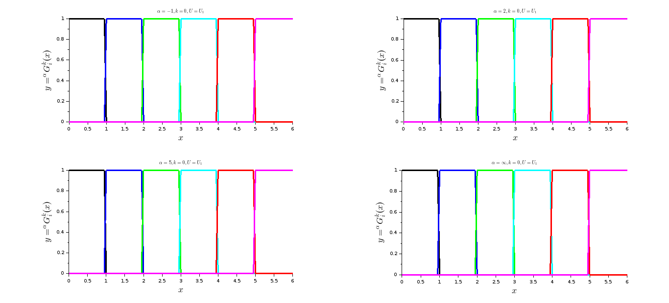
Figure 4: The B-spline basis $\displaystyle{{{}^{\alpha}}{\bf G}_{i}^{0}}$ of knot vector $U_{0}$

Figure 5: The B-spline basis $\displaystyle{{{}^{\alpha}}{\bf G}_{i}^{1}}$ of knot vector $U_{0}$

Figure 6: The B-spline basis $\displaystyle{{{}^{\alpha}}{\bf G}_{i}^{2}}$ of knot vector $U_{0}$

Figure 7: The B-spline basis $\displaystyle{{{}^{\alpha}}{\bf G}_{i}^{3}}$ of knot vector $U_{0}$

From the analysis of figures 4 to 7, we deduce that since $U_{0}$ is a uniform periodic knot vector, an element of the basis $\displaystyle{{\left({{{}^{\alpha}}{\bf G}_{i}^{k}}\right)}_{i=0}^{m-k-1}}$ is obtained by simple translation of $\displaystyle{{{}^{\alpha}}{\bf G}_{0}^{k}}$ that is $\displaystyle{{{}^{\alpha}}{\bf G}_{i}^{k}(x)={{}^{\alpha}}{\bf G}_{0}^{k}(t_{0}-t_{i}+x)}$.

We observe that $\displaystyle{{{\bf supp}\,{{}^{\alpha}}{\bf G}_{i}^{k}}={\left[{t_{i}}\,,\,{t_{i+k+1}}\right]}}$ and also the effect of parameter $\alpha$ is crucial at the neighborhood of $0^{-}$ and $1^{+}$. The figure 7 seems to show that $\alpha$ does not have any influence on $\displaystyle{{\left({{{}^{\alpha}}{\bf G}_{i}^{3}}\right)}_{i=0}^{m-4}}$ which corresponds to a context of knot vector with no interior nodes.

Illustration 5.2

We present the influence of the non-uniformity of a periodic knot vector by restricting ourselves on B-spline basis of degree $2$ in the following cases:

$\displaystyle{U_{1}=\left(0,1,2,3,3,5,6\right)}$

$\displaystyle{U_{2}=\left(0,1,1,2,4,5,6\right)}$

$\displaystyle{U_{3}=\left(0,1,1.5,2,3.5,5,6\right)}$

Figure 8: The B-spline basis $\displaystyle{{{}^{\alpha}}{\bf G}_{i}^{2}}$ of knot vector $U_{1}$

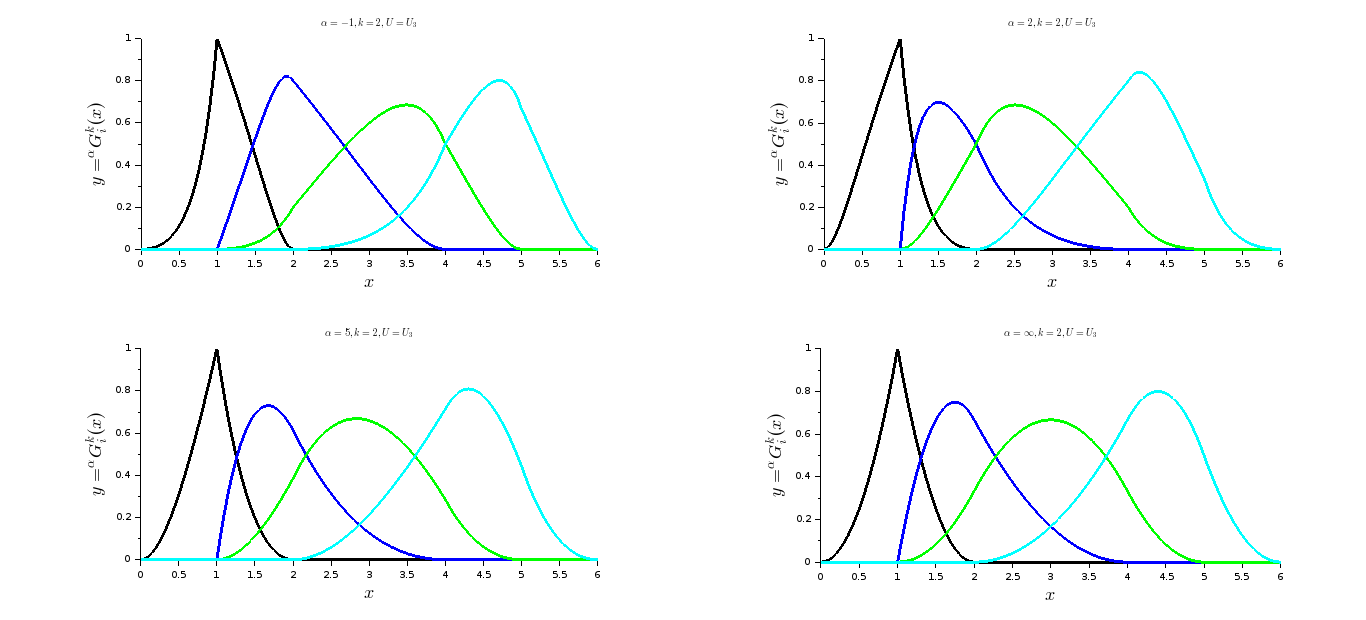
Figure 9: The B-spline basis $\displaystyle{{{}^{\alpha}}{\bf G}_{i}^{2}}$ of knot vector $U_{2}$

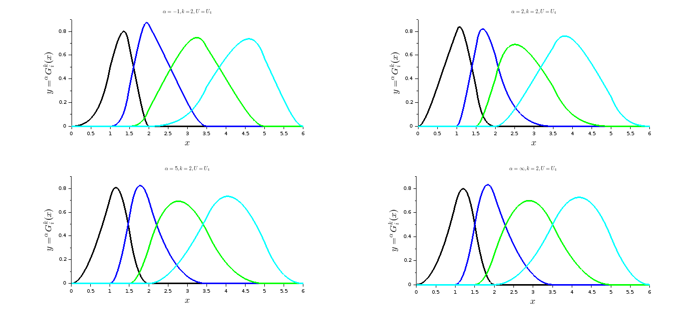
Figure 10: The B-spline basis $\displaystyle{{{}^{\alpha}}{\bf G}_{i}^{2}}$ of knot vector $U_{3}$

The non-uniformity may come from the presence of a multiple node, it is the case of knot vectors $U_{1}$ and $U_{2}$. It may be also due to the step of variable between nodes as in $U_{3}$.

The figures 8 to 10 show that in all the cases we have $\displaystyle{{{\bf supp}\,{{}^{\alpha}}{\bf G}_{i}^{2}}={\left[{t_{i}}\,,\,{t_{i+3}}\right]}}$ and the effect of the parameter $\alpha$ remains important at the neighborhood of $0^{-}$ and $1^{+}$. We observe a large diversity among the elements of the basis concerning the regularity.

The two illustrations of this subsection seem to confirm the conjecture 3.1 related to the existence of a unique maximum for $\displaystyle{{{}^{\alpha}}{\bf G}_{i}^{k}}$ when $k>0$.

5.1.2 Case of open knot vectors

This subsection is also based on two test cases which give light on the basis of degree $2$ generated by open knot vectors for $\displaystyle{\alpha\in\{-1,2,5,\infty\}}$.

The first test case dealts with five knot vectors having two multiple interior nodes or not.

In the second test case we also have five knot vectors but having three interior nodes where the multiplicity may reach $3$.

Illustration 5.3

We explore the case of B-spline basis of degree $2$ associated with an open knot vector in the following cases:

$\displaystyle{U_{4}=\left(0,0,0,1,2,3,3,3\right)}$

$\displaystyle{U_{5}=\left(0,0,0,0.4,2.6,3,3,3\right)}$

$\displaystyle{U_{6}=\left(0,0,0,1.8,2.2,3,3,3\right)}$

$\displaystyle{U_{7}=\left(0,0,0,1,1,3,3,3\right)}$

$\displaystyle{U_{8}=\left(0,0,0,2,2,3,3,3\right)}$

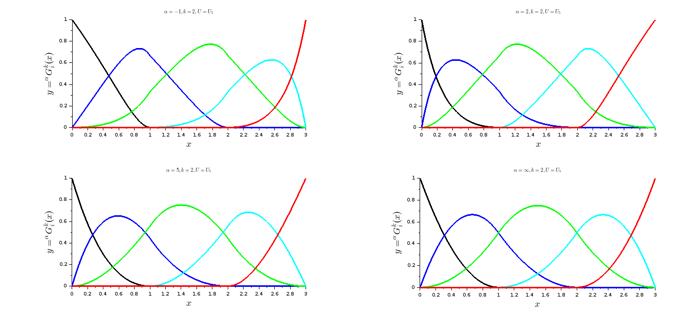
Figure 11: The B-spline basis $\displaystyle{{{}^{\alpha}}{\bf G}_{i}^{2}}$ of knot vector $U_{4}$

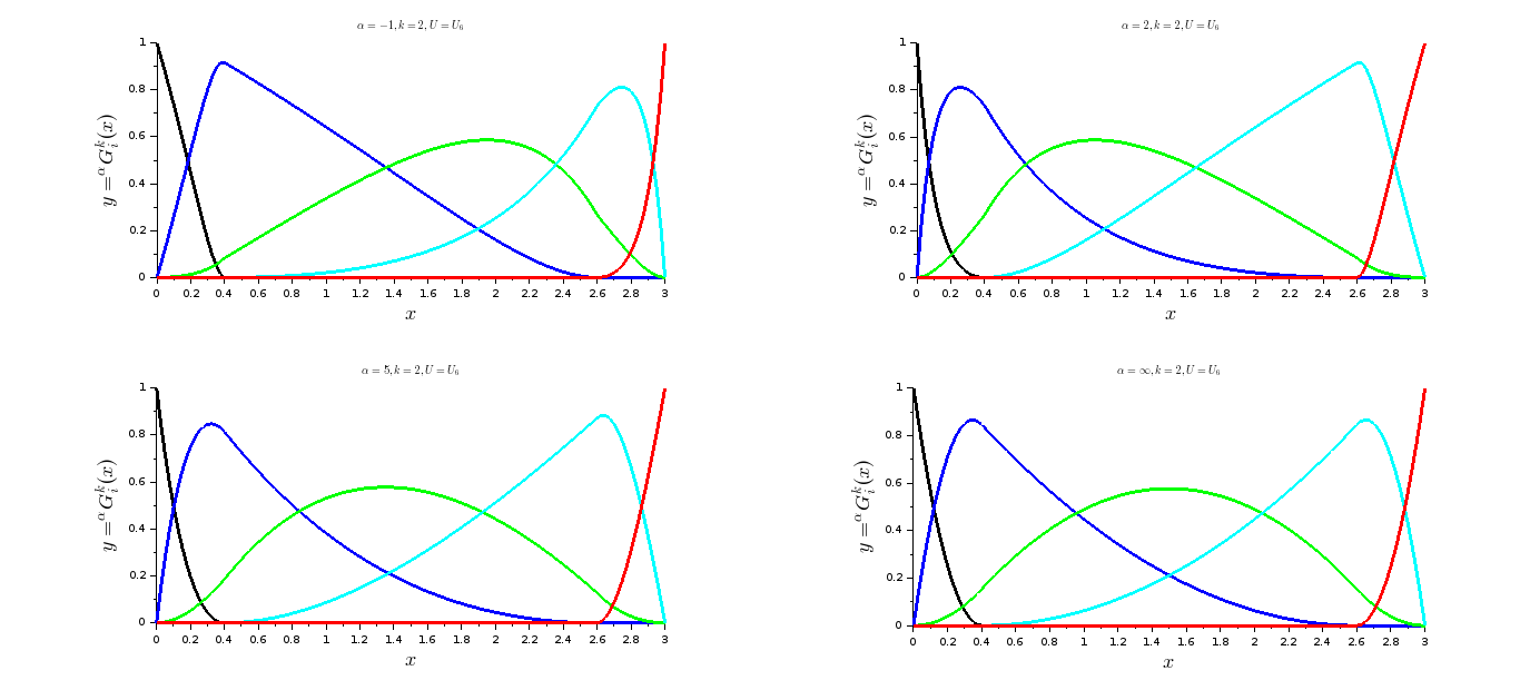
Figure 12: The B-spline basis $\displaystyle{{{}^{\alpha}}{\bf G}_{i}^{2}}$ of knot vector $U_{5}$

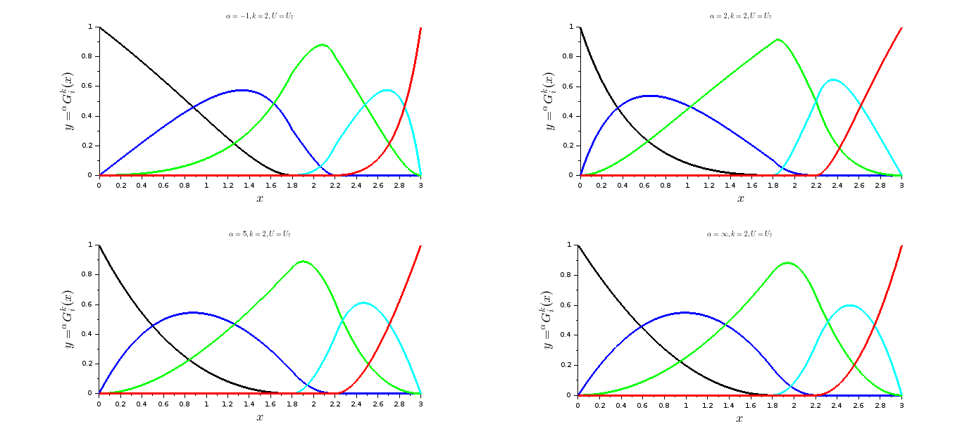
Figure 13: The B-spline basis $\displaystyle{{{}^{\alpha}}{\bf G}_{i}^{2}}$ of knot vector $U_{6}$

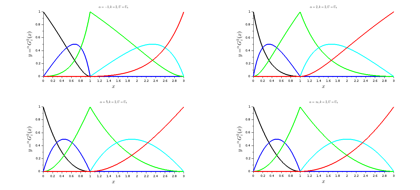
Figure 14: The B-spline basis $\displaystyle{{{}^{\alpha}}{\bf G}_{i}^{2}}$ of knot vector $U_{7}$

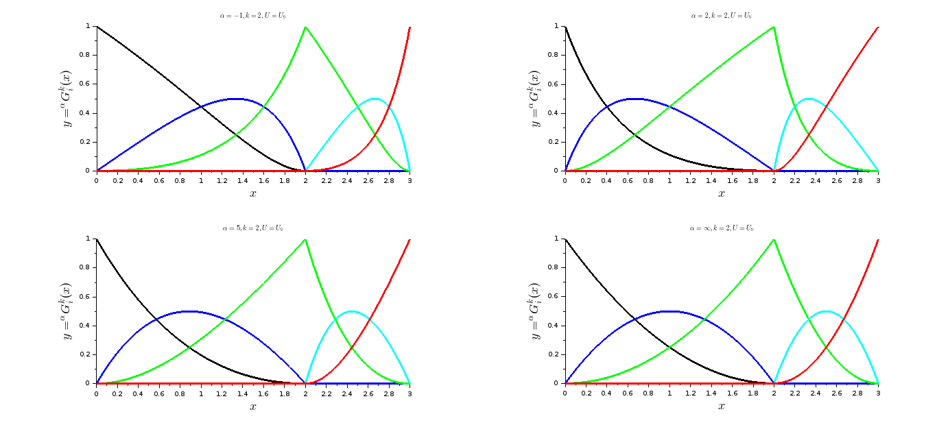
Figure 15: The B-spline basis $\displaystyle{{{}^{\alpha}}{\bf G}_{i}^{2}}$ of knot vector $U_{8}$

The figures 11 to 15 illustrate abundantly the properties of the proposition 3.2 especially those of values at extreme nodes.

The figures 11 and 12 depict the behaviors of basis generated respectively by $U_{4}$ and $U_{5}$ which are symmetric knot vectors. One can observe that for all $x\in{\left[{t_{0}}\,,\,{t_{7}}\right]}$, we have

$$\begin{array}[]{l}\displaystyle{{{}^{-1}}{\bf G}_{i}^{2}(t_{0}+t_{7}-x)={{}^{2}}{\bf G}_{4-i}^{2}(x)}\\ \displaystyle{{{}^{2}}{\bf G}_{i}^{2}(t_{0}+t_{7}-x)={{}^{-1}}{\bf G}_{4-i}^{2}(x)}\\ \displaystyle{{{}^{\infty}}{\bf G}_{i}^{2}(t_{0}+t_{7}-x)={{}^{\infty}}{\bf G}_{4-i}^{2}(x)}\\ \end{array}$$

For the non-uniform open knot vector $U_{6}$, $U_{7}$ and $U_{8}$ we observe a large diversity of behaviors of generated basis.

Illustration 5.4

The B-spline basis of degree $2$ we are illustrating explore the existing relation between the regularity and the multiplicity of an interior node of an open knot vector in the following cases:

$\displaystyle{U_{9}=\left(0,0,0,3/4,6/4,9/4,3,3,3\right)}$

$\displaystyle{U_{10}=\left(0,0,0,3/4,3/4,9/4,3,3,3\right)}$

$\displaystyle{U_{11}=\left(0,0,0,3/4,3/4,3/4,3,3,3\right)}$

$\displaystyle{U_{12}=\left(0,0,0,3/4,9/4,9/4,3,3,3\right)}$

$\displaystyle{U_{13}=\left(0,0,0,9/4,9/4,9/4,3,3,3\right)}$

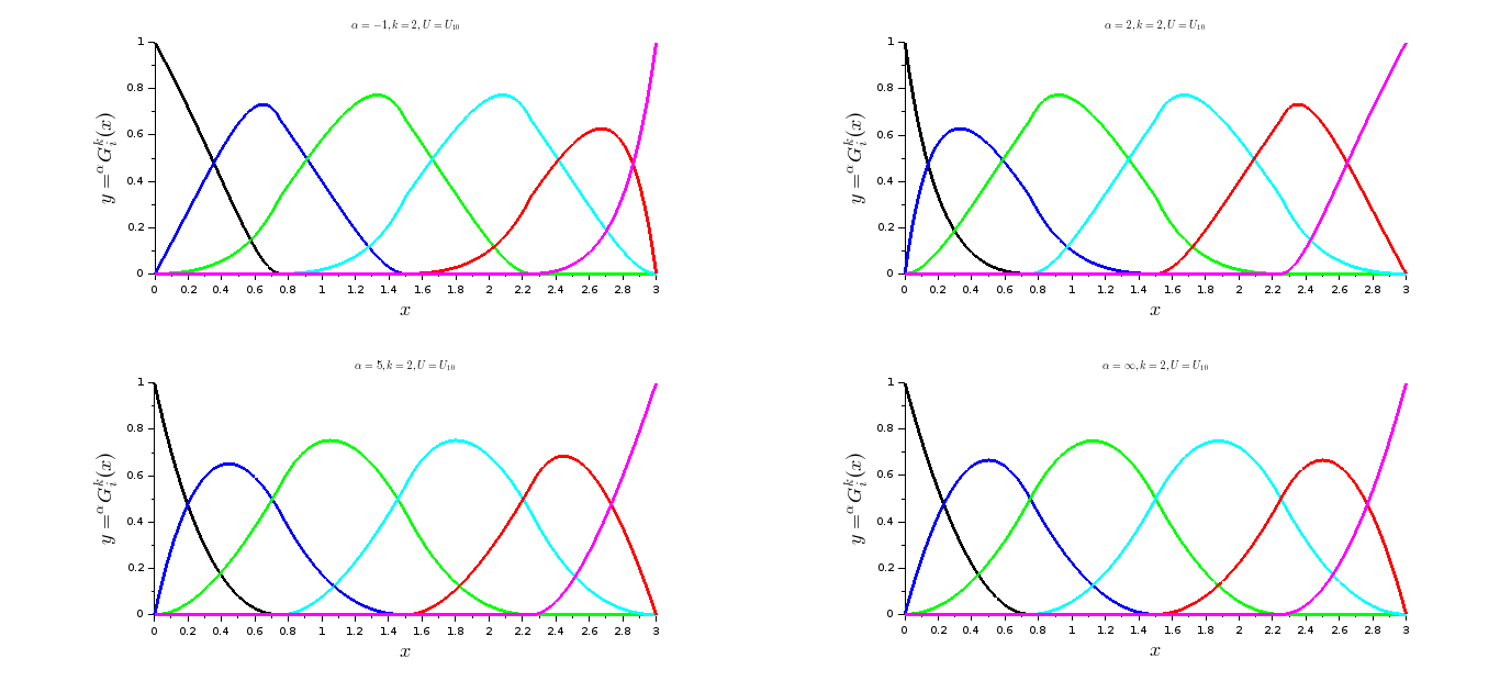
Figure 16: The B-spline basis $\displaystyle{{{}^{\alpha}}{\bf G}_{i}^{2}}$ of knot vector $U_{9}$

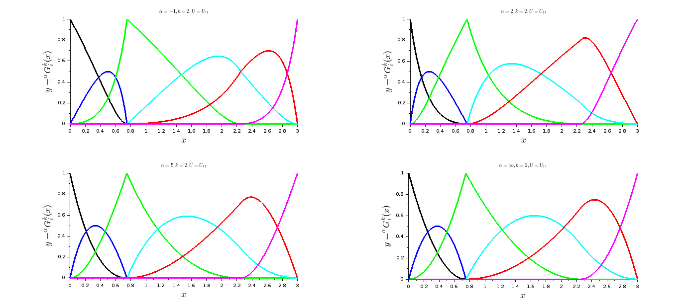
Figure 17: The B-spline basis $\displaystyle{{{}^{\alpha}}{\bf G}_{i}^{2}}$ of knot vector $U_{10}$

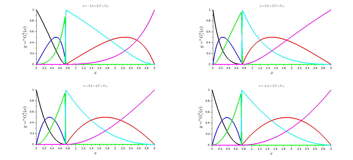
Figure 18: The B-spline basis $\displaystyle{{{}^{\alpha}}{\bf G}_{i}^{2}}$ of knot vector $U_{11}$

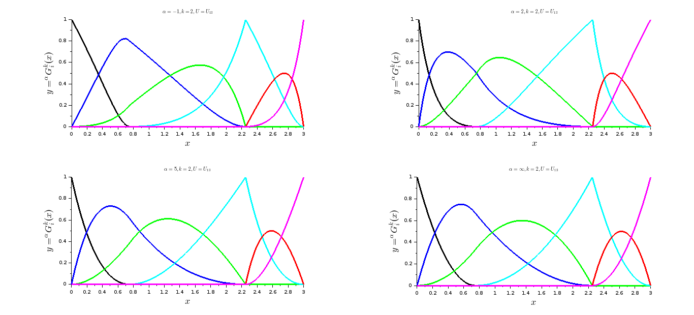
Figure 19: The B-spline basis $\displaystyle{{{}^{\alpha}}{\bf G}_{i}^{2}}$ of knot vector $U_{12}$

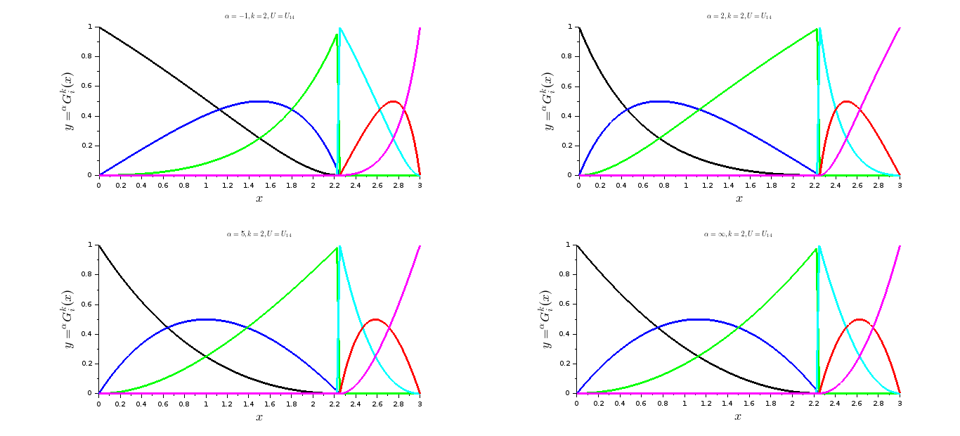
Figure 20: The B-spline basis $\displaystyle{{{}^{\alpha}}{\bf G}_{i}^{2}}$ of knot vector $U_{13}$

The knot vector $U_{9}$ is uniform with interior nodes of multiplicity $1$ and we observe in figure 16 that the generated basis confirms the behaviors we already observed with $U_{4}$. We can state their regularity of ${\cal C}^{0}$ as well as the left and right differentiability at any interior node as provided in proposition 3.3.

Each of the knot vectors $U_{10}$ and $U_{12}$ has one interior node with multiplicity $2$. The analysis of figures 17 and 19 shows that the associated basis $\displaystyle{{{}^{\alpha}}{\bf G}_{i}^{2}}$ are at least of ${\cal C}^{0}$ with the existence of a left and right derivatives at any interior node even at a double node confirming the results in proposition 3.3.

Each of the knot vectors $U_{11}$ and $U_{13}$ has one interior triple node $t_{3}=t_{4}=t_{5}$. We must expect a first type of discontinuity for the elements $\displaystyle{{{}^{\alpha}}{\bf G}_{2}^{2}}$ and $\displaystyle{{{}^{\alpha}}{\bf G}_{3}^{2}}$ of the associated basis as $\displaystyle{{{\bf supp}\,{{}^{\alpha}}{\bf G}_{2}^{2}}={\left[{t_{2}}\,,\,{t_{5}}\right]}}$ and $\displaystyle{{{\bf supp}\,{{}^{\alpha}}{\bf G}_{3}^{2}}={\left[{t_{3}}\,,\,{t_{6}}\right]}}$. The other elements of the basis keep the regularity of ${\cal C}^{0}$ with the existence of a left and right derivatives at any interior node. This is confirmed by the analysis of figures 18 and 20.

Remark 5.1

Either the knot vector is periodic or open, uinform or not, we observe in all the cases that $\displaystyle{{{}^{\infty}}{\bf G}_{i}^{2}\approx{{}^{5}}{\bf G}_{i}^{2}}$ and the conjecture 3.1 is verified.

5.2 The new class of rational B-spline curves

Let us have a look on some examples showing the behavior of new B-spline curves under the effect of various parameter appearing in their definition.

Amongst some parameters we can refer to index $\alpha$, the degree $k$, the knot vector $U$ and the control polygon $\Pi$.

Illustration 5.5

Let begin with the new parameter which is the index $\alpha$. We fix the degree to $3$ on the uniform and open knot vector $U$ and the control polygon $\Pi$ as follows:

$\displaystyle{U=\left(0,0,0,0,1,2,3,4,5,5,5,5\right)}$

$\displaystyle{\Pi=\left\{{\left({0}\,,\,{2}\right)},{\left({1.5}\,,\,{5}\right)},{\left({2.5}\,,\,{4}\right)},{\left({3}\,,\,{1}\right)},{\left({5}\,,\,{4}\right)},{\left({7}\,,\,{1}\right)},{\left({8}\,,\,{4}\right)},{\left({10}\,,\,{4}\right)}\right\}}$

We will go through $\displaystyle{\alpha\in\{-\infty,-4,-1/2,-1/5,-1/7\}}$, as well as its conjugated $1-\alpha$.

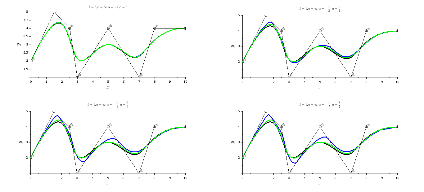
Figure 21: Influence of $\alpha$ to $k=3$, $U$ uniform and open with fixed $\Pi$

A quick analysis of figure 21 reveals:

1. For $\displaystyle{\alpha\leq-4}$ and $\displaystyle{\alpha\geq 5}$, the B-spline curve $\displaystyle{G_{\alpha}}$ of degree $k$ and index $\alpha$ is a good approximationof the standard polynomial B-spline curve $\displaystyle{G_{\infty}}$ generated by the same control polygon $\Pi$.

2. When $\alpha$ tends to $0^{-}$ or to $1^{+}$, the curve $\displaystyle{G_{\alpha}}$ is really separated from the standard curve $\displaystyle{G_{\infty}}$. The effect seems more viewed at the neighborhood of $0$ but the question is still to be tackled later on.

3. We reach a conclusion that the B-spline curves family becomes more interesting.

Illustration 5.6

The second important parameter is the degree $k$ of the basis which generates the B-spline curve. We will observe its influence on two examples discribed by the following data where the control polygon $\Pi_{i}$ has been fixed with a uniform and open knot vector $U_{i,k}$ giving the degree $k$ as follows:

1. Example 1

   $\displaystyle{\Pi_{1}=\left\{{\left({0}\,,\,{0}\right)},{\left({3}\,,\,{9}\right)},{\left({6}\,,\,{3}\right)},{\left({9}\,,\,{6}\right)}\right\}}$

   $\displaystyle{U_{1,1}=\left(0,0,1,2,3,3\right)}$

   $\displaystyle{U_{1,2}=\left(0,0,0,1.5,3,3,3\right)}$

   $\displaystyle{U_{1,3}=\left(0,0,0,0,3,3,3,3\right)}$

2. Example 2

   $\displaystyle{\Pi_{2}=\left\{{\left({1}\,,\,{3}\right)},{\left({0}\,,\,{5}\right)},{\left({5}\,,\,{5}\right)},{\left({3}\,,\,{0}\right)},{\left({8}\,,\,{0}\right)},{\left({7}\,,\,{3}\right)}\right\}}$

   $\displaystyle{U_{2,1}=\left(0,0,1,2,3,4,5,5\right)}$

   $\displaystyle{U_{2,2}=\left(0,0,0,5/4,5/2,15/4,5,5,5\right)}$

   $\displaystyle{U_{2,3}=\left(0,0,0,0,5/3,10/3,5,5,5,5\right)}$

   $\displaystyle{U_{2,4}=\left(0,0,0,0,0,5/2,5,5,5,5,5\right)}$

   $\displaystyle{U_{2,5}=\left(0,0,0,0,0,0,5,5,5,5,5,5\right)}$

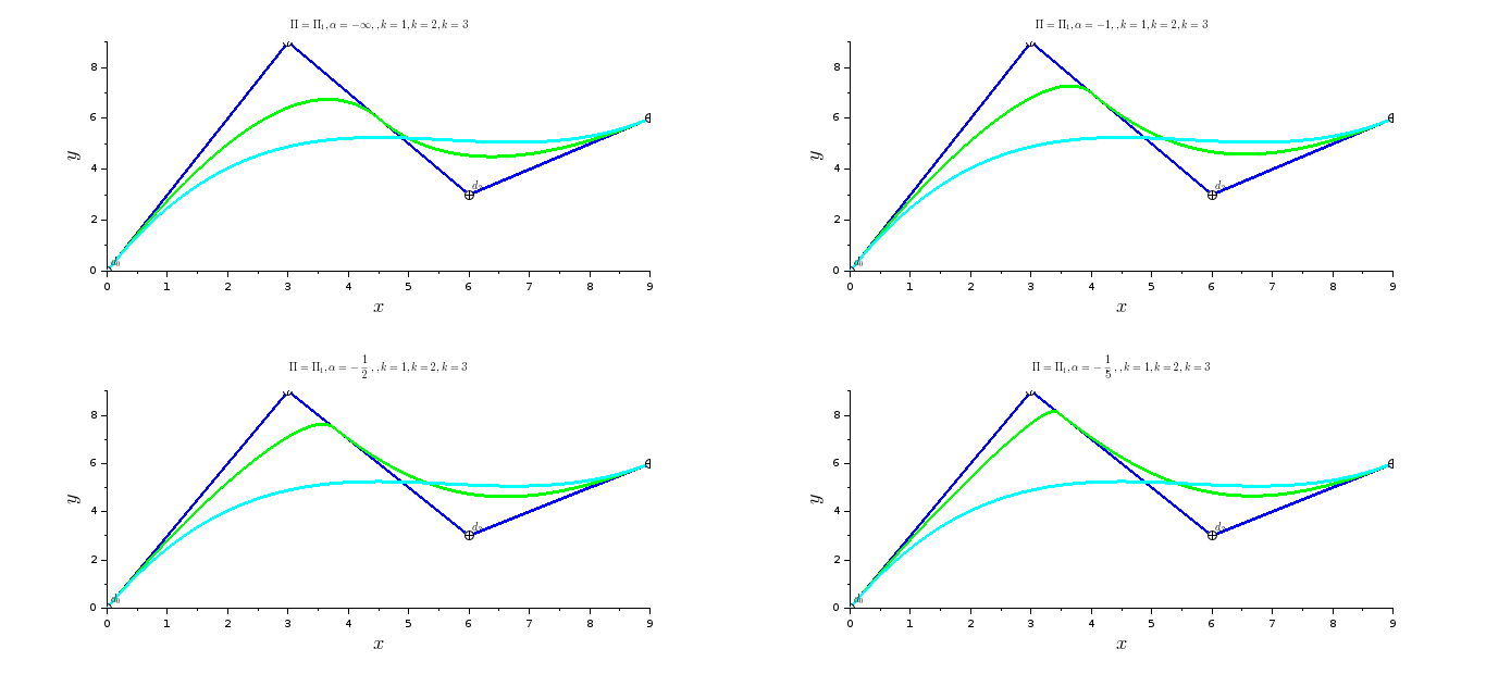
Figure 22: Influence of degree $k$, $U$ uniform and open at $\alpha$ with fixed $\Pi$

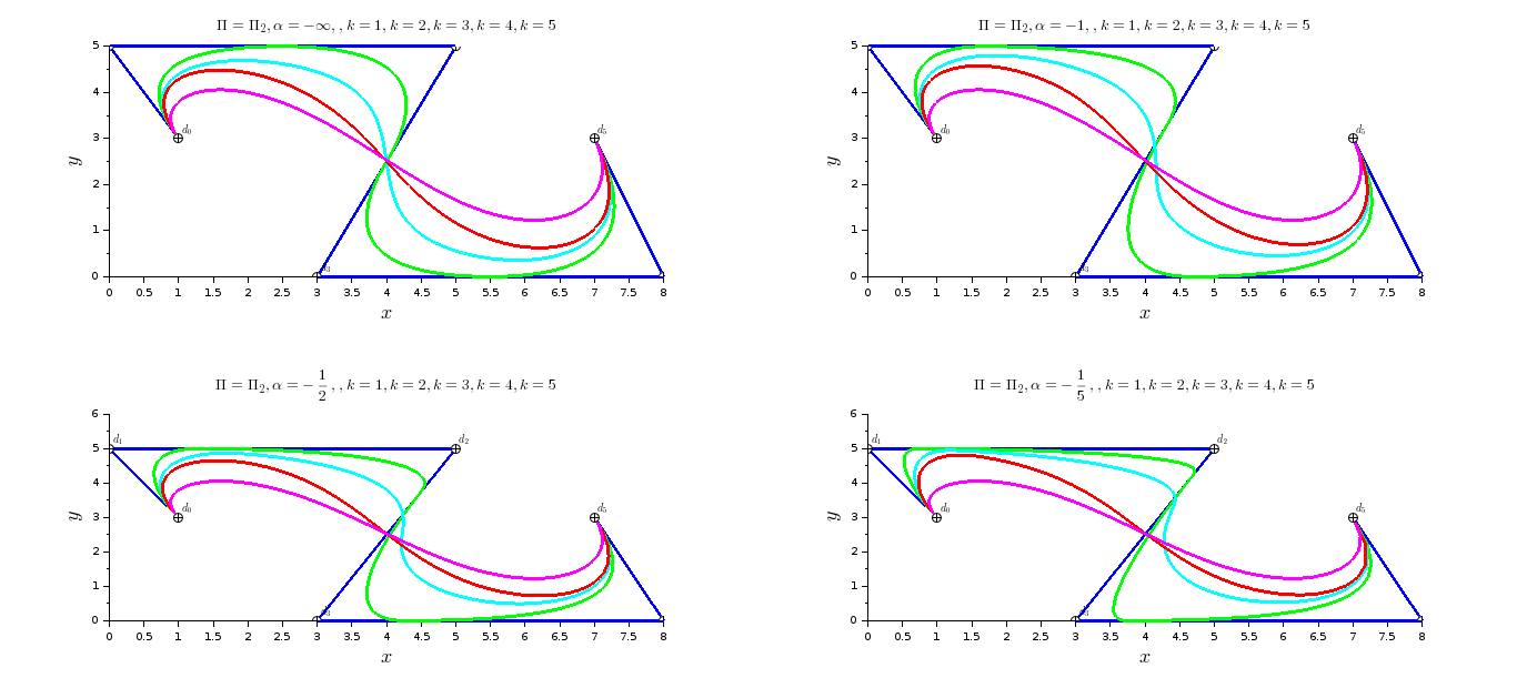
Figure 23: Influence of degree $k$, $U$ uniform and open at $\alpha$ with fixed $\Pi$

The figure 22 summarizes example 1 and show on one hand that independently from $\alpha$, the degree $k=1$ yields the control polygon $\Pi$. On the other hand, $k=3$ corresponds to a knot vector without any interior node and the obtained B-spline curve $\displaystyle{G_{\alpha}}$ is independent from $\alpha$. Only the degree $k=2$ between the extremes undergo the influence of index $\alpha$ with some highlight when $\alpha$ tends to $0$.

The results of example 2 shown in figure 23 confirm above observations.

The degree $k=1$ yields the control polygon $\Pi_{2}$ and the degree $k=5$ which corresponds to a knot vector with no interior node does not have any influence under $\alpha$. For the intermediate degrees $k$ the index $\alpha$ has an incresing influence when $\alpha$ tends to $0$.

Illustration 5.7

Now we intend to look at the influence of control polygon $\Pi$ on the local behavior of a B-spline curve. We fix the degree to $3$ on the uniform and open knot vector $U$ by varing only one point of the control polygon as follows:

$\displaystyle{U=\left(0,0,0,0,1,2,3,4,4,4,4\right)}$

$\displaystyle{\Pi_{1}=\left\{{\left({0}\,,\,{4}\right)},{\left({5}\,,\,{4}\right)},{\left({5}\,,\,{8}\right)},{\left({11}\,,\,{7.5}\right)},{\left({6}\,,\,{2}\right)},{\left({12}\,,\,{0}\right)},{\left({2}\,,\,{0}\right)}\right\}}$

$\displaystyle{\Pi_{2}=\left\{{\left({0}\,,\,{4}\right)},{\left({5}\,,\,{4}\right)},{\left({5}\,,\,{8}\right)},{\left({11}\,,\,{7.5}\right)},{\left({9}\,,\,{3}\right)},{\left({12}\,,\,{0}\right)},{\left({2}\,,\,{0}\right)}\right\}}$

$\displaystyle{\Pi_{3}=\left\{{\left({0}\,,\,{4}\right)},{\left({5}\,,\,{4}\right)},{\left({5}\,,\,{8}\right)},{\left({11}\,,\,{7.5}\right)},{\left({12}\,,\,{4}\right)},{\left({12}\,,\,{0}\right)},{\left({2}\,,\,{0}\right)}\right\}}$

We take $\displaystyle{\alpha\in\{-\infty,-4,-1/2,-1/5,-1/7\}}$, as well as its conjugated $1-\alpha$.

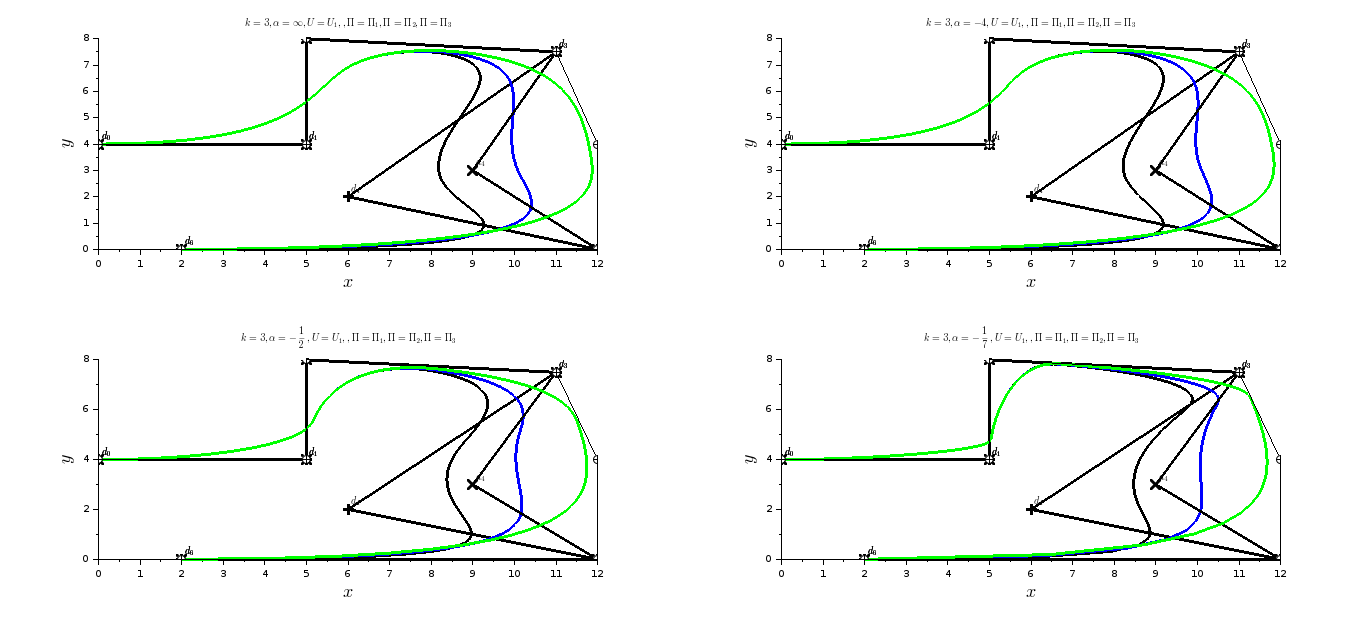
Figure 24: Influence of the variation of a point of $\Pi$ at $k=3$, $U$ uniform and open and $\alpha\in\{-\infty,-4,-1/2,-1/5,-1/7\}$

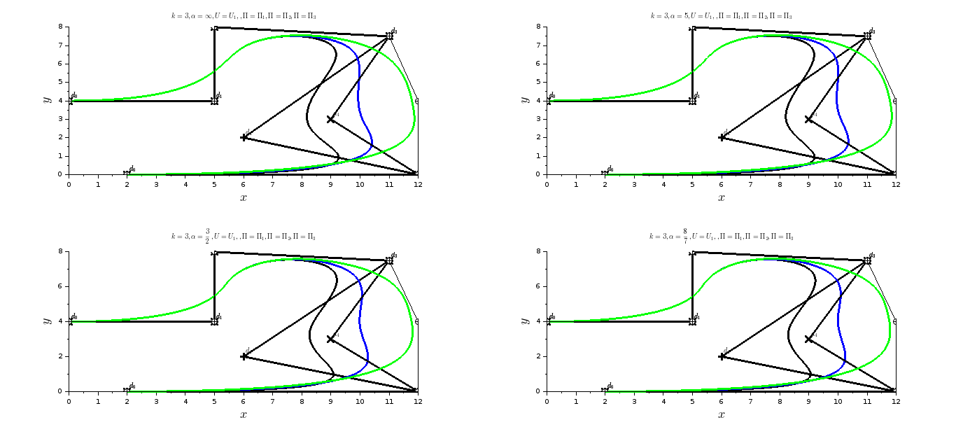
Figure 25: Influence of the variation of a point of $\Pi$ at $k=3$, $U$ uniform and open and $\alpha\in\{\infty,5,3/2,6/5,8/7\}$

Figures 24 and 25 let us to state that each curve $\displaystyle{G_{\alpha}}$ is made up of three segments where the second one is under the motion of the fifth endpoint of the control polygon $\Pi$. As we have noted so far, the influence of $\alpha$ is not so remarkable for $\alpha\leq-4$ and $\alpha\geq 5$ as one can note in polynomial case that is to say $\displaystyle{G_{\alpha}\approx G_{\infty}}$.

In the deformation region of the curve $\displaystyle{G_{\alpha}}$ at the neighborhood of a segment $\displaystyle{{\left[{d_{i}}\,,\,{d_{i+1}}\right]}}$ of control polygon $\Pi_{j}$, the deformation moves towards the point $\displaystyle{d_{i}}$ when $\displaystyle{\alpha\in(-1\,,\,0)}$ and towards the point $\displaystyle{d_{i+1}}$ when $\displaystyle{\alpha\in(1\,,\,2)}$ as shown in figures 24 and 25 respectively. In all cases, the curve $\displaystyle{G_{\alpha}}$ belongs to the convex envelop of the control polygon $\Pi_{j}$.

Remark 5.2

Through the figure 21 of illustration 5.5 and figures 22 and 23 of illustration 5.6 as well as figures 24 and 25 of illustration 5.7, we realize that the property of convex envelop is widely verified.

Illustration 5.8

In this test case, we will explore the property of symmetry proved in proposition 4.3 through seven contexts where we restrict ourselves to an axis of symmetry parallel to the coordinate axes which does not reduce generality. The data are as follow:

1. Axial symmetry of $\Pi$ with axis parallel to Oy with no multiple point

   $\displaystyle{\Pi_{1}=\left\{\begin{array}[]{l}{\left({4}\,,\,{0}\right)},{\left({0}\,,\,{11}\right)},{\left({6}\,,\,{14}\right)},\\ {\left({10}\,,\,{14}\right)},{\left({16}\,,\,{11}\right)},{\left({12}\,,\,{0}\right)}\\ \end{array}\right\}}$

   $\displaystyle{U_{1}=\left(0,0,0,0,1,2,3,3,3,3\right)}$

2. Axial symmetry of $\Pi$ with axis parallel to Oy with one double point

   $\displaystyle{\Pi_{2}=\left\{\begin{array}[]{l}{\left({4}\,,\,{0}\right)},{\left({0}\,,\,{11}\right)},{\left({8}\,,\,{14}\right)},\\ {\left({8}\,,\,{14}\right)},{\left({16}\,,\,{11}\right)},{\left({12}\,,\,{0}\right)}\\ \end{array}\right\}}$

   $\displaystyle{U_{2}=\left(0,0,0,0,1,2,3,3,3,3\right)}$

3. Axial symmetry of $\Pi$ with axis parallel to Oy with double point and double node

   $\displaystyle{\Pi_{3}=\left\{\begin{array}[]{l}{\left({4}\,,\,{0}\right)},{\left({0}\,,\,{11}\right)},{\left({8}\,,\,{14}\right)},\\ {\left({8}\,,\,{14}\right)},{\left({16}\,,\,{11}\right)},{\left({12}\,,\,{0}\right)}\\ \end{array}\right\}}$

   $\displaystyle{U_{3}=\left(0,0,0,0,2,2,4,4,4,4\right)}$

4. Axial symmetry of $\Pi$ with axis parallel to Ox with no multiple point

   $\displaystyle{\Pi_{4}=\left\{\begin{array}[]{l}{\left({0}\,,\,{5}\right)},{\left({0}\,,\,{4}\right)},{\left({1}\,,\,{4}\right)},\\ {\left({2}\,,\,{4}\right)},{\left({2}\,,\,{6}\right)},{\left({4}\,,\,{6}\right)},{\left({5}\,,\,{5}\right)},\\ {\left({5}\,,\,{1}\right)},{\left({4}\,,\,{0}\right)},{\left({2}\,,\,{0}\right)},\\ {\left({2}\,,\,{2}\right)},{\left({1}\,,\,{2}\right)},{\left({0}\,,\,{2}\right)},{\left({0}\,,\,{1}\right)}\\ \end{array}\right\}}$

   $\displaystyle{U_{4}=\left(0,0,0,0,1,2,3,4,5,6,7,8,9,10,11,11,11,11\right)}$

5. Axial symmetry of $\Pi$ with axis parallel to Ox with double point

   $\displaystyle{\Pi_{5}=\left\{\begin{array}[]{l}{\left({0}\,,\,{5}\right)},{\left({0}\,,\,{4}\right)},{\left({1}\,,\,{4}\right)},\\ {\left({2}\,,\,{4}\right)},{\left({2}\,,\,{6}\right)},{\left({4}\,,\,{6}\right)},{\left({5}\,,\,{3}\right)},\\ {\left({5}\,,\,{3}\right)},{\left({4}\,,\,{0}\right)},{\left({2}\,,\,{0}\right)},\\ {\left({2}\,,\,{2}\right)},{\left({1}\,,\,{2}\right)},{\left({0}\,,\,{2}\right)},{\left({0}\,,\,{1}\right)}\\ \end{array}\right\}}$

   $\displaystyle{U_{5}=\left(0,0,0,0,1,2,3,4,5,6,7,8,9,10,11,11,11,11\right)}$

6. Axial symmetry of $\Pi$ with axis parallel to Ox with double point and double node

   $\displaystyle{\Pi_{6}=\left\{\begin{array}[]{l}{\left({0}\,,\,{5}\right)},{\left({0}\,,\,{4}\right)},{\left({1}\,,\,{4}\right)},\\ {\left({2}\,,\,{4}\right)},{\left({2}\,,\,{6}\right)},{\left({4}\,,\,{6}\right)},{\left({5}\,,\,{3}\right)},\\ {\left({5}\,,\,{3}\right)},{\left({4}\,,\,{0}\right)},{\left({2}\,,\,{0}\right)},\\ {\left({2}\,,\,{2}\right)},{\left({1}\,,\,{2}\right)},{\left({0}\,,\,{2}\right)},{\left({0}\,,\,{1}\right)}\\ \end{array}\right\}}$

   $\displaystyle{U_{6}=\left(0,0,0,0,1,2,3,4,5,5,6,7,8,9,10,10,10,10\right)}$

7. Double axial symmetry of $\Pi$ with one double point

   $\displaystyle{\Pi_{7}=\left\{\begin{array}[]{l}{\left({0}\,,\,{2}\right)},{\left({0}\,,\,{3}\right)},{\left({1}\,,\,{4}\right)},\\ {\left({3}\,,\,{4}\right)},{\left({5}\,,\,{4}\right)},{\left({6}\,,\,{3}\right)},\\ {\left({6}\,,\,{2}\right)},{\left({6}\,,\,{1}\right)},{\left({5}\,,\,{0}\right)},\\ {\left({3}\,,\,{0}\right)},{\left({1}\,,\,{0}\right)},{\left({0}\,,\,{1}\right)},{\left({0}\,,\,{2}\right)}\\ \end{array}\right\}}$

   $\displaystyle{U_{7}=\left(0,0,0,0,1,2,3,4,5,6,7,8,9,10,10,10,10\right)}$

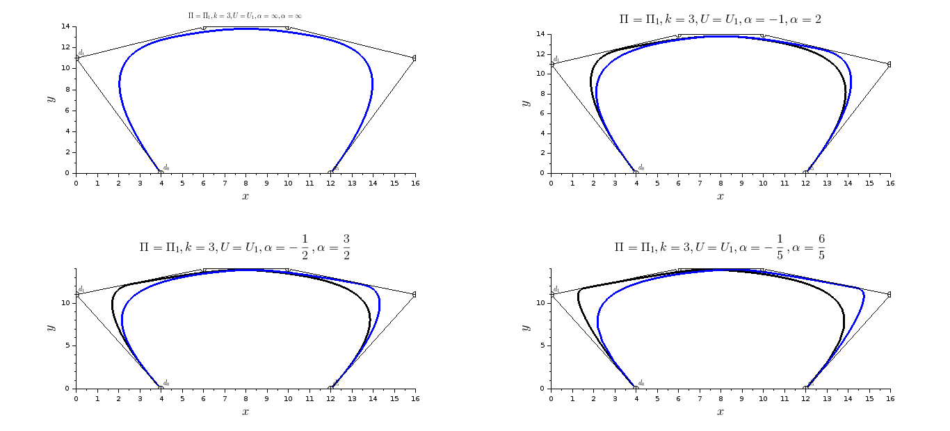
Figure 26: $\displaystyle{G_{\alpha}}$ curves of degree $k=3$, $U_{1}$ uniform and open, $\Pi_{1}$ symmetric with no multiple point and $\alpha\in\{\infty,-1,-1/2,-1/5\}$

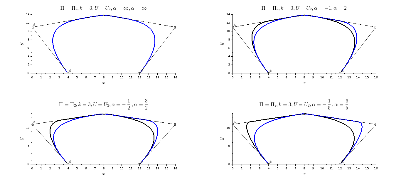
Figure 27: $\displaystyle{G_{\alpha}}$ curves of degree $k=3$, $U_{2}$ uniform and open, $\Pi_{2}$ symmetric with double point and $\alpha\in\{\infty,-1,-1/2,-1/5\}$

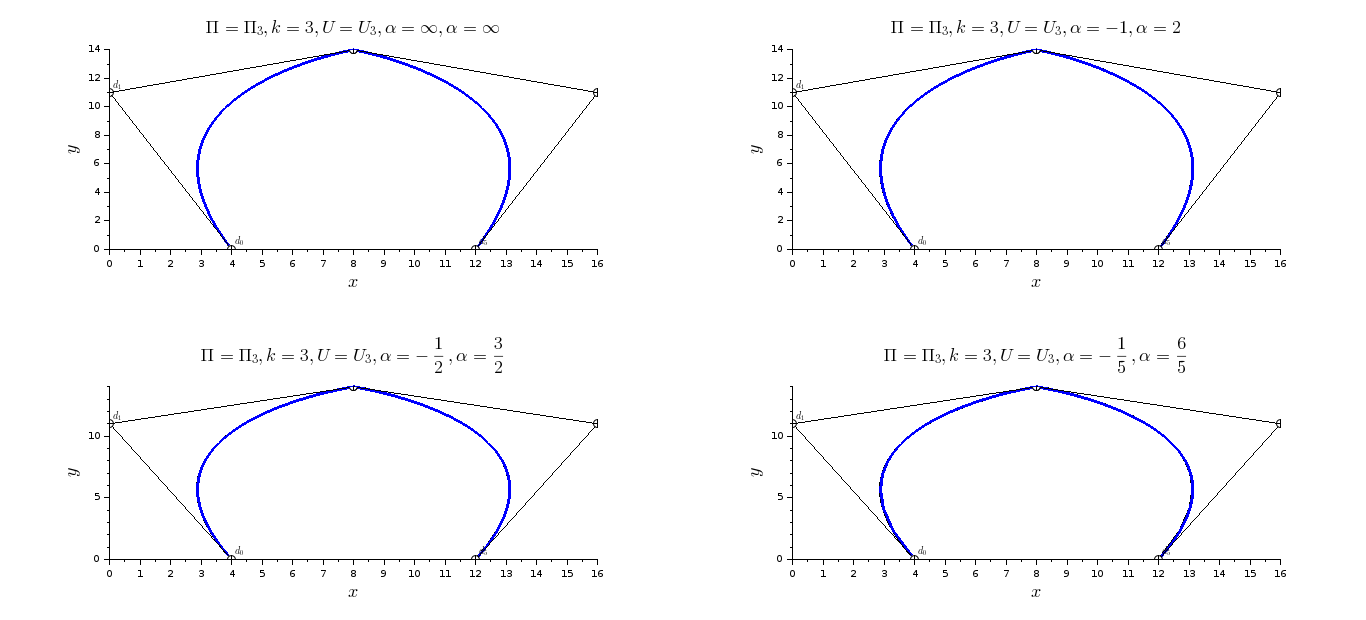
Figure 28: $\displaystyle{G_{\alpha}}$ curves of degree $k=3$, $U_{3}$ symmetric and open with double node, $\Pi_{3}$ symmetric with double point and $\alpha\in\{\infty,-1,-1/2,-1/5\}$

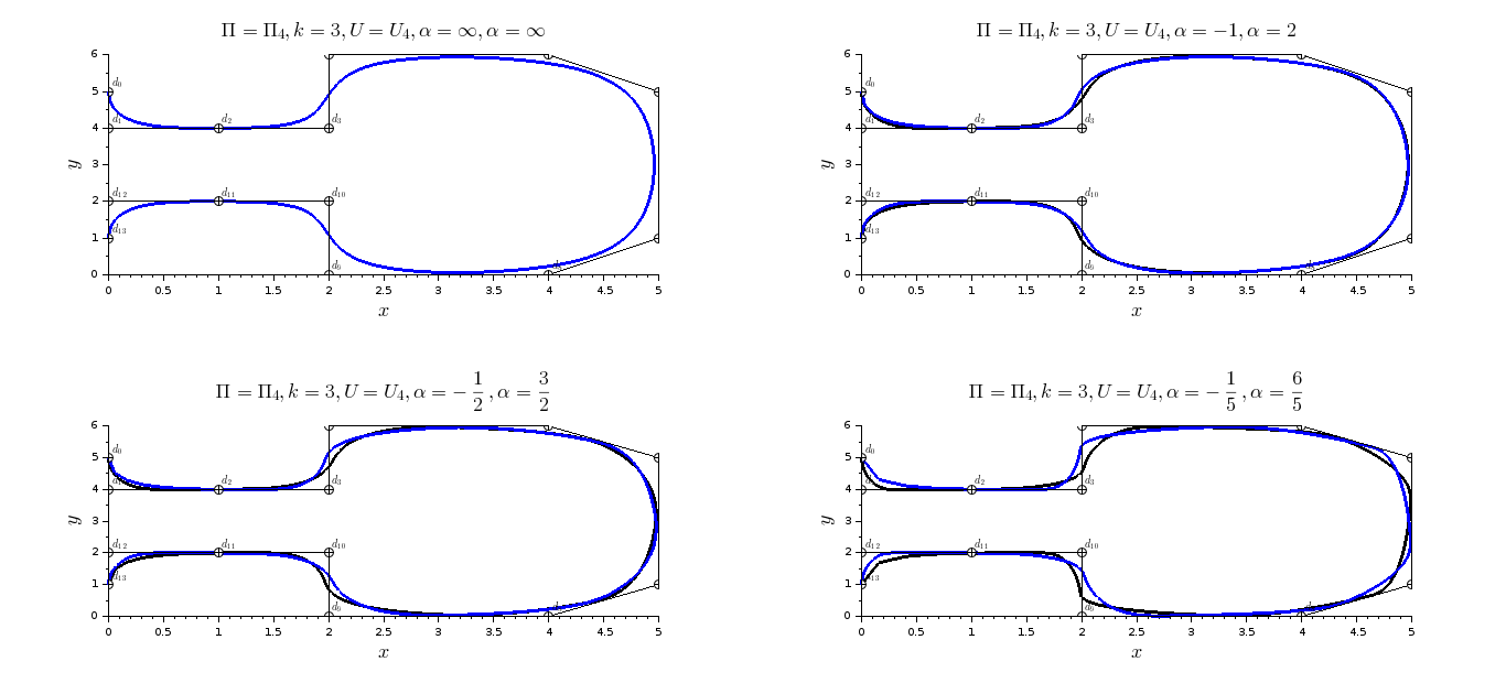
Figure 29: $\displaystyle{G_{\alpha}}$ curves of degree $k=3$, $U_{4}$ uniform and open, $\Pi_{4}$ symmetric with no multiple point and $\alpha\in\{\infty,-1,-1/2,-1/5\}$

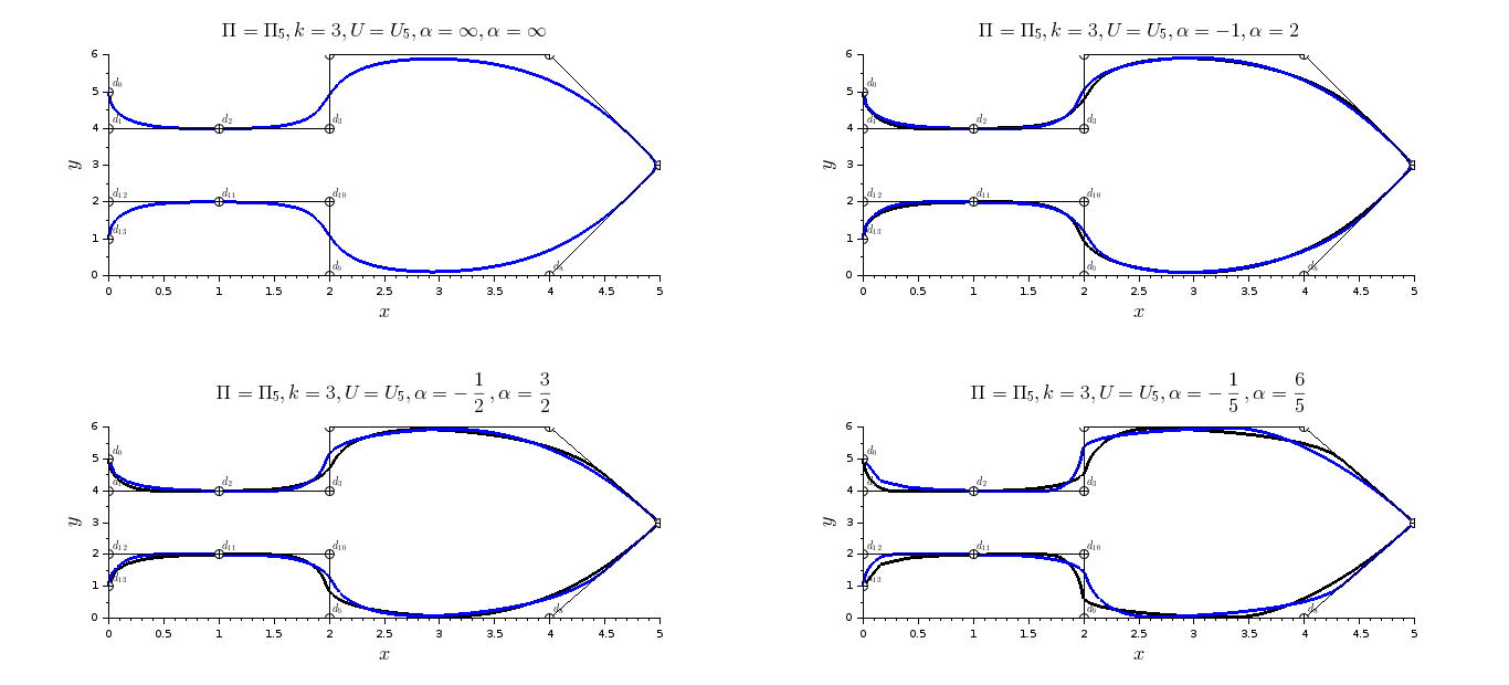
Figure 30: $\displaystyle{G_{\alpha}}$ curves of degree $k=3$, $U_{5}$ uniform and open, $\Pi_{5}$ symmetric with double point and $\alpha\in\{\infty,-1,-1/2,-1/5\}$

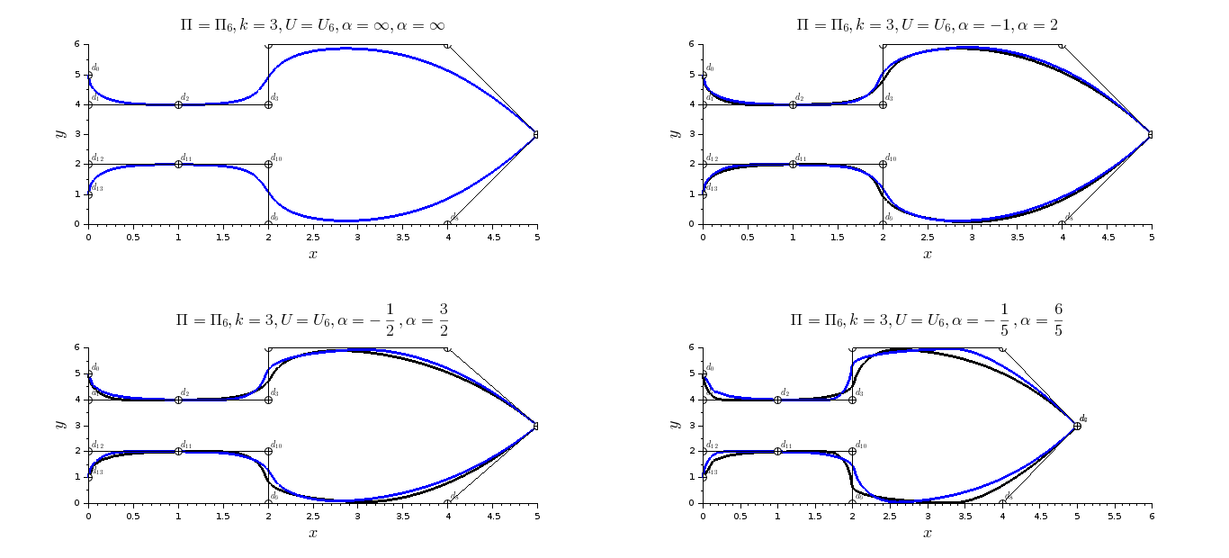
Figure 31: $\displaystyle{G_{\alpha}}$ curves of degree $k=3$, $U_{6}$ symmetric and open with double node, $\Pi_{6}$ symmetric with double point and $\alpha\in\{\infty,-1,-1/2,-1/5\}$

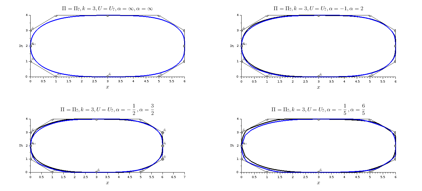
Figure 32: $\displaystyle{G_{\alpha}}$ curves of degree $k=3$, $U_{7}$ uniform and open, $\Pi_{7}$ symmetric with double point and $\alpha\in\{\infty,-1,-1/2,-1/5\}$

Based on figures from 26 to 32, it can be drawn that the curves $\displaystyle{G_{\alpha}}$ and $\displaystyle{G_{1-\alpha}}$ are symmetric with respect to the perpendicular bisector of extreme points of the control polygon $\Pi$. As stated above, the effect àf index $\alpha$ is very remarkable for $\displaystyle{\alpha\in(-1\,,\,0)\cup(1\,,\,2)}$.

The multiplicity of a node acts on the geometrical regularity of curves $\displaystyle{G_{\alpha}}$ and $\displaystyle{G_{1-\alpha}}$. In the presence of a double control point, the curves $\displaystyle{G_{\alpha}}$ and $\displaystyle{G_{1-\alpha}}$ adhere to this point.

The figure 28 shows however a singular case which we will light upon later on since $\alpha$ seems to have no influence on it.

6 Conclusion

The class of parametrization we developed allows us to construct a family of rational B-spline basis depending on a parameter $\alpha$ which generalizes all including polynomial B-spline basis. This new family of B-spline basis possesses all the classical fundamental properties such as positivity, unit partition property and linear independence. Some symmetry property has been established.

We have proved that the family of B-spline curves we obtained is larger than the polynomial B-spline curves one and globally extend their properties. Illustrations are given to explain more the properties we proved with the desire of the extension to practical computation algorithms of curves (deBoor algorithm) in future work.

It is left with the exploration in more details of the effect of this new parametrization on Bernstein functions and the resulting Bézier curves.

Appendix

This section shows results extracted from outputs processed by a Maxima code.

B-spline basis of degree 2 and its derivative for the knot vector

$U=\left(x_{0},x_{0},x_{0},x_{1},x_{2},x_{2},x_{2}\right)$

$${{}^{\alpha}}{\bf G}_{i}^{2}(t)=\left\{\begin{array}[]{ll}{{\left(\alpha-1\right)^{2}\,\left({\it x_{1}}-t\right)^{2}}\over{\left(\alpha\,{\it x_{1}}-{\it x_{1}}-\alpha\,{\it x_{0}}+t\right)^{2}}}&\textrm{if }i=0\textrm{ and }t\in[x_{0}\,,\,x_{1}[\\ -\frac{\left(\alpha-1\right)\,\alpha\,\left({\it x_{0}}-t\right)}{{\left(\alpha\,{\it x_{1}}-{\it x_{1}}-\alpha\,{\it x_{0}}+t\right)^{2}\,\left(\alpha\,{\it x_{2}}-{\it x_{2}}-\alpha\,{\it x_{0}}+t\right)}}\times&\\ \left[2\,\alpha\,{\it x_{1}}\,{\it x_{2}}-2\,{\it x_{1}}\,{\it x_{2}}-\alpha\,{\it x_{0}}\,{\it x_{2}}\right.&\\ \left.-\alpha\,t\,{\it x_{2}}+2\,t\,{\it x_{2}}-\alpha\,{\it x_{0}}\,{\it x_{1}}-\alpha\,t\,{\it x_{1}}\right.&\\ \left.+2\,t\,{\it x_{1}}+2\,\alpha\,t\,{\it x_{0}}-2\,t^{2}\right]&\textrm{if }i=1\textrm{ and }t\in[x_{0}\,,\,x_{1}[\\ {{\left(\alpha-1\right)^{2}\,\left({\it x_{2}}-t\right)^{2}}\over{\left(\alpha\,{\it x_{2}}-{\it x_{2}}-\alpha\,{\it x_{0}}+t\right)\,\left(\alpha\,{\it x_{2}}-{\it x_{2}}-\alpha\,{\it x_{1}}+t\right)}}&\textrm{if }i=1\textrm{ and }t\in[x_{1}\,,\,x_{2}[\\ {{\alpha^{2}\,\left({\it x_{0}}-t\right)^{2}}\over{\left(\alpha\,{\it x_{1}}-{\it x_{1}}-\alpha\,{\it x_{0}}+t\right)\,\left(\alpha\,{\it x_{2}}-{\it x_{2}}-\alpha\,{\it x_{0}}+t\right)}}&\textrm{if }i=2\textrm{ and }t\in[x_{0}\,,\,x_{1}[\\ -\frac{\left(\alpha-1\right)\,\alpha\,\left({\it x_{2}}-t\right)}{{\left(\alpha\,{\it x_{2}}-{\it x_{2}}-\alpha\,{\it x_{0}}+t\right)\,\left(\alpha\,{\it x_{2}}-{\it x_{2}}-\alpha\,{\it x_{1}}+t\right)^{2}}}\times&\\ \left(\alpha\,{\it x_{1}}\,{\it x_{2}}-{\it x_{1}}\,{\it x_{2}}+\alpha\,{\it x_{0}}\,{\it x_{2}}-{\it x_{0}}\,{\it x_{2}}\right.&\\ \left.-2\,\alpha\,t\,{\it x_{2}}+2\,t\,{\it x_{2}}-2\,\alpha\,{\it x_{0}}\,{\it x_{1}}+\alpha\,t\,{\it x_{1}}+t\,{\it x_{1}}\right.&\\ \left.+\alpha\,t\,{\it x_{0}}+t\,{\it x_{0}}-2\,t^{2}\right)&\textrm{if }i=2\textrm{ and }t\in[x_{1}\,,\,x_{2}[\\ {{\alpha^{2}\,\left({\it x_{1}}-t\right)^{2}}\over{\left(\alpha\,{\it x_{2}}-{\it x_{2}}-\alpha\,{\it x_{1}}+t\right)^{2}}}&\textrm{if }i=3\textrm{ and }t\in[x_{1}\,,\,x_{2}[\\ 0&\textrm{otherwise }\\ \end{array}\right.$$

$$\frac{d}{dt}{{}^{\alpha}}{\bf G}_{i}^{2}(t)=\left\{\begin{array}[]{ll}\displaystyle{-{{2\,\left(\alpha-1\right)^{2}\,\alpha\,\left({\it x_{1}}-t\right)\,\left({\it x_{1}}-{\it x_{0}}\right)}\over{\left(\alpha\,{\it x_{1}}-{\it x_{1}}-\alpha\,{\it x_{0}}+t\right)^{3}}}}&\textrm{if }i=0\textrm{ and }t\in[x_{0}\,,\,x_{1}[\\ \displaystyle{\frac{\left(\alpha-1\right)\,\alpha}{{\left(\alpha\,{\it x_{1}}-{\it x_{1}}-\alpha\,{\it x_{0}}+t\right)^{3}\,\left(\alpha\,{\it x_{2}}-{\it x_{2}}-\alpha\,{\it x_{0}}+t\right)^{2}}}\times}&\\ \left[2\,\alpha^{3}\,{\it x_{1}}^{2}\,{\it x_{2}}^{2}-6\,\alpha^{2}\,{\it x_{1}}^{2}\,{\it x_{2}}^{2}+6\,\alpha\,{\it x_{1}}^{2}\,{\it x_{2}}^{2}\right.&\\ \left.-2\,{\it x_{1}}^{2}\,{\it x_{2}}^{2}-2\,\alpha^{3}\,{\it x_{0}}\,{\it x_{1}}\,{\it x_{2}}^{2}+6\,\alpha^{2}\,{\it x_{0}}\,{\it x_{1}}\,{\it x_{2}}^{2}\right.&\\ \left.-6\,\alpha\,{\it x_{0}}\,{\it x_{1}}\,{\it x_{2}}^{2}+2\,{\it x_{0}}\,{\it x_{1}}\,{\it x_{2}}^{2}-2\,\alpha^{3}\,t\,{\it x_{1}}\,{\it x_{2}}^{2}\right.&\\ \left.+6\,\alpha^{2}\,t\,{\it x_{1}}\,{\it x_{2}}^{2}-6\,\alpha\,t\,{\it x_{1}}\,{\it x_{2}}^{2}+2\,t\,{\it x_{1}}\,{\it x_{2}}^{2}\right.&\\ \left.+2\,\alpha^{3}\,t\,{\it x_{0}}\,{\it x_{2}}^{2}-6\,\alpha^{2}\,t\,{\it x_{0}}\,{\it x_{2}}^{2}+6\,\alpha\,t\,{\it x_{0}}\,{\it x_{2}}^{2}\right.&\\ \left.-2\,t\,{\it x_{0}}\,{\it x_{2}}^{2}-2\,\alpha^{3}\,{\it x_{0}}\,{\it x_{1}}^{2}\,{\it x_{2}}+4\,\alpha^{2}\,{\it x_{0}}\,{\it x_{1}}^{2}\,{\it x_{2}}\right.&\\ \left.-2\,\alpha\,{\it x_{0}}\,{\it x_{1}}^{2}\,{\it x_{2}}-2\,\alpha^{3}\,t\,{\it x_{1}}^{2}\,{\it x_{2}}+8\,\alpha^{2}\,t\,{\it x_{1}}^{2}\,{\it x_{2}}\right.&\\ \left.-10\,\alpha\,t\,{\it x_{1}}^{2}\,{\it x_{2}}+4\,t\,{\it x_{1}}^{2}\,{\it x_{2}}-3\,\alpha^{2}\,{\it x_{0}}^{2}\,{\it x_{1}}\,{\it x_{2}}\right.&\\ \left.+3\,\alpha\,{\it x_{0}}^{2}\,{\it x_{1}}\,{\it x_{2}}+8\,\alpha^{3}\,t\,{\it x_{0}}\,{\it x_{1}}\,{\it x_{2}}-14\,\alpha^{2}\,t\,{\it x_{0}}\,{\it x_{1}}\,{\it x_{2}}\right.&\\ \left.+10\,\alpha\,t\,{\it x_{0}}\,{\it x_{1}}\,{\it x_{2}}-4\,t\,{\it x_{0}}\,{\it x_{1}}\,{\it x_{2}}-7\,\alpha^{2}\,t^{2}\,{\it x_{1}}\,{\it x_{2}}\right.&\\ \left.+11\,\alpha\,t^{2}\,{\it x_{1}}\,{\it x_{2}}-4\,t^{2}\,{\it x_{1}}\,{\it x_{2}}+2\,\alpha^{3}\,{\it x_{0}}^{3}\,{\it x_{2}}-\alpha^{2}\,{\it x_{0}}^{3}\,{\it x_{2}}\right.&\\ \left.-6\,\alpha^{3}\,t\,{\it x_{0}}^{2}\,{\it x_{2}}+6\,\alpha^{2}\,t\,{\it x_{0}}^{2}\,{\it x_{2}}-3\,\alpha\,t\,{\it x_{0}}^{2}\,{\it x_{2}}\right.&\\ \left.+7\,\alpha^{2}\,t^{2}\,{\it x_{0}}\,{\it x_{2}}-8\,\alpha\,t^{2}\,{\it x_{0}}\,{\it x_{2}}+4\,t^{2}\,{\it x_{0}}\,{\it x_{2}}\right.&\\ \left.-\alpha\,t^{3}\,{\it x_{2}}+\alpha^{2}\,{\it x_{0}}^{2}\,{\it x_{1}}^{2}-\alpha\,{\it x_{0}}^{2}\,{\it x_{1}}^{2}+2\,\alpha^{3}\,t\,{\it x_{0}}\,{\it x_{1}}^{2}\right.&\\ \left.-6\,\alpha^{2}\,t\,{\it x_{0}}\,{\it x_{1}}^{2}+4\,\alpha\,t\,{\it x_{0}}\,{\it x_{1}}^{2}-\alpha^{2}\,t^{2}\,{\it x_{1}}^{2}\right.&\\ \left.+3\,\alpha\,t^{2}\,{\it x_{1}}^{2}-2\,t^{2}\,{\it x_{1}}^{2}+2\,\alpha^{3}\,{\it x_{0}}^{3}\,{\it x_{1}}-\alpha^{2}\,{\it x_{0}}^{3}\,{\it x_{1}}\right.&\\ \left.-6\,\alpha^{3}\,t\,{\it x_{0}}^{2}\,{\it x_{1}}+4\,\alpha^{2}\,t\,{\it x_{0}}^{2}\,{\it x_{1}}-\alpha\,t\,{\it x_{0}}^{2}\,{\it x_{1}}\right.&\\ \left.+9\,\alpha^{2}\,t^{2}\,{\it x_{0}}\,{\it x_{1}}-8\,\alpha\,t^{2}\,{\it x_{0}}\,{\it x_{1}}+2\,t^{2}\,{\it x_{0}}\,{\it x_{1}}-3\,\alpha\,t^{3}\,{\it x_{1}}\right.&\\ \left.+2\,t^{3}\,{\it x_{1}}-2\,\alpha^{3}\,{\it x_{0}}^{4}+4\,\alpha^{3}\,t\,{\it x_{0}}^{3}+2\,\alpha^{2}\,t\,{\it x_{0}}^{3}\right.&\\ \left.-8\,\alpha^{2}\,t^{2}\,{\it x_{0}}^{2}+2\,\alpha\,t^{2}\,{\it x_{0}}^{2}+4\,\alpha\,t^{3}\,{\it x_{0}}-2\,t^{3}\,{\it x_{0}}\right]&\textrm{if }i=1\textrm{ and }t\in[x_{0}\,,\,x_{1}[\\ \end{array}\right.$$

$$\frac{d}{dt}{{}^{\alpha}}{\bf G}_{i}^{2}(t)=\left\{\begin{array}[]{ll}\displaystyle{-\frac{\left(\alpha-1\right)^{2}\,\alpha\,\left({\it x_{2}}-t\right)}{{\left(\alpha\,{\it x_{2}}-{\it x_{2}}-\alpha\,{\it x_{0}}+t\right)^{2}\,\left(\alpha\,{\it x_{2}}-{\it x_{2}}-\alpha\,{\it x_{1}}+t\right)^{2}}}\times}&\\ \left[2\,\alpha\,{\it x_{2}}^{2}-2\,{\it x_{2}}^{2}-2\,\alpha\,{\it x_{1}}\,{\it x_{2}}+{\it x_{1}}\,{\it x_{2}}-2\,\alpha\,{\it x_{0}}\,{\it x_{2}}+{\it x_{0}}\,{\it x_{2}}\right.&\\ \left.+2\,t\,{\it x_{2}}+2\,\alpha\,{\it x_{0}}\,{\it x_{1}}-t\,{\it x_{1}}-t\,{\it x_{0}}\right]&\textrm{if }i=1\textrm{ and }t\in[x_{1}\,,\,x_{2}[\\ \displaystyle{-\frac{\left(\alpha-1\right)\,\alpha^{2}\,\left({\it x_{0}}-t\right)}{{\left(\alpha\,{\it x_{1}}-{\it x_{1}}-\alpha\,{\it x_{0}}+t\right)^{2}\,\left(\alpha\,{\it x_{2}}-{\it x_{2}}-\alpha\,{\it x_{0}}+t\right)^{2}}}\times}&\\ \left[2\,\alpha\,{\it x_{1}}\,{\it x_{2}}-2\,{\it x_{1}}\,{\it x_{2}}-2\,\alpha\,{\it x_{0}}\,{\it x_{2}}+{\it x_{0}}\,{\it x_{2}}\right.&\\ \left.+t\,{\it x_{2}}-2\,\alpha\,{\it x_{0}}\,{\it x_{1}}+{\it x_{0}}\,{\it x_{1}}+t\,{\it x_{1}}+2\,\alpha\,{\it x_{0}}^{2}-2\,t\,{\it x_{0}}\right]&\textrm{if }i=2\textrm{ and }t\in[x_{0}\,,\,x_{1}[\\ \displaystyle{\frac{\left(\alpha-1\right)\,\alpha}{{\left(\alpha\,{\it x_{2}}-{\it x_{2}}-\alpha\,{\it x_{0}}+t\right)^{2}\,\left(\alpha\,{\it x_{2}}-{\it x_{2}}-\alpha\,{\it x_{1}}+t\right)^{3}}}\times}&\\ \left[2\,\alpha^{3}\,{\it x_{2}}^{4}-6\,\alpha^{2}\,{\it x_{2}}^{4}+6\,\alpha\,{\it x_{2}}^{4}-2\,{\it x_{2}}^{4}-2\,\alpha^{3}\,{\it x_{1}}\,{\it x_{2}}^{3}\right.&\\ \left.+5\,\alpha^{2}\,{\it x_{1}}\,{\it x_{2}}^{3}-4\,\alpha\,{\it x_{1}}\,{\it x_{2}}^{3}+{\it x_{1}}\,{\it x_{2}}^{3}-2\,\alpha^{3}\,{\it x_{0}}\,{\it x_{2}}^{3}\right.&\\ \left.+5\,\alpha^{2}\,{\it x_{0}}\,{\it x_{2}}^{3}-4\,\alpha\,{\it x_{0}}\,{\it x_{2}}^{3}+{\it x_{0}}\,{\it x_{2}}^{3}-4\,\alpha^{3}\,t\,{\it x_{2}}^{3}\right.&\\ \left.+14\,\alpha^{2}\,t\,{\it x_{2}}^{3}-16\,\alpha\,t\,{\it x_{2}}^{3}+6\,t\,{\it x_{2}}^{3}+\alpha^{2}\,{\it x_{1}}^{2}\,{\it x_{2}}^{2}\right.&\\ \left.-\alpha\,{\it x_{1}}^{2}\,{\it x_{2}}^{2}-3\,\alpha^{2}\,{\it x_{0}}\,{\it x_{1}}\,{\it x_{2}}^{2}+3\,\alpha\,{\it x_{0}}\,{\it x_{1}}\,{\it x_{2}}^{2}+6\,\alpha^{3}\,t\,{\it x_{1}}\,{\it x_{2}}^{2}\right.&\\ \left.-14\,\alpha^{2}\,t\,{\it x_{1}}\,{\it x_{2}}^{2}+11\,\alpha\,t\,{\it x_{1}}\,{\it x_{2}}^{2}-3\,t\,{\it x_{1}}\,{\it x_{2}}^{2}+6\,\alpha^{3}\,t\,{\it x_{0}}\,{\it x_{2}}^{2}\right.&\\ \left.-12\,\alpha^{2}\,t\,{\it x_{0}}\,{\it x_{2}}^{2}+9\,\alpha\,t\,{\it x_{0}}\,{\it x_{2}}^{2}-3\,t\,{\it x_{0}}\,{\it x_{2}}^{2}-8\,\alpha^{2}\,t^{2}\,{\it x_{2}}^{2}\right.&\\ \left.+14\,\alpha\,t^{2}\,{\it x_{2}}^{2}-6\,t^{2}\,{\it x_{2}}^{2}+2\,\alpha^{3}\,{\it x_{0}}\,{\it x_{1}}^{2}\,{\it x_{2}}-2\,\alpha^{3}\,t\,{\it x_{1}}^{2}\,{\it x_{2}}\right.&\\ \left.+2\,\alpha\,t\,{\it x_{1}}^{2}\,{\it x_{2}}+2\,\alpha^{3}\,{\it x_{0}}^{2}\,{\it x_{1}}\,{\it x_{2}}-8\,\alpha^{3}\,t\,{\it x_{0}}\,{\it x_{1}}\,{\it x_{2}}\right.&\\ \left.+10\,\alpha^{2}\,t\,{\it x_{0}}\,{\it x_{1}}\,{\it x_{2}}-6\,\alpha\,t\,{\it x_{0}}\,{\it x_{1}}\,{\it x_{2}}+9\,\alpha^{2}\,t^{2}\,{\it x_{1}}\,{\it x_{2}}\right.&\\ \left.-10\,\alpha\,t^{2}\,{\it x_{1}}\,{\it x_{2}}+3\,t^{2}\,{\it x_{1}}\,{\it x_{2}}-2\,\alpha^{3}\,t\,{\it x_{0}}^{2}\,{\it x_{2}}+7\,\alpha^{2}\,t^{2}\,{\it x_{0}}\,{\it x_{2}}\right.&\\ \left.-6\,\alpha\,t^{2}\,{\it x_{0}}\,{\it x_{2}}+3\,t^{2}\,{\it x_{0}}\,{\it x_{2}}-4\,\alpha\,t^{3}\,{\it x_{2}}+2\,t^{3}\,{\it x_{2}}\right.&\\ \left.-2\,\alpha^{3}\,{\it x_{0}}^{2}\,{\it x_{1}}^{2}+2\,\alpha^{3}\,t\,{\it x_{0}}\,{\it x_{1}}^{2}+2\,\alpha^{2}\,t\,{\it x_{0}}\,{\it x_{1}}^{2}-\alpha^{2}\,t^{2}\,{\it x_{1}}^{2}\right.&\\ \left.-\alpha\,t^{2}\,{\it x_{1}}^{2}+2\,\alpha^{3}\,t\,{\it x_{0}}^{2}\,{\it x_{1}}-7\,\alpha^{2}\,t^{2}\,{\it x_{0}}\,{\it x_{1}}\right.&\\ \left.+3\,\alpha\,t^{2}\,{\it x_{0}}\,{\it x_{1}}+3\,\alpha\,t^{3}\,{\it x_{1}}-t^{3}\,{\it x_{1}}+\alpha\,t^{3}\,{\it x_{0}}-t^{3}\,{\it x_{0}}\right]&\textrm{if }i=2\textrm{ and }t\in[x_{1}\,,\,x_{2}[\\ \displaystyle{-{{2\,\left(\alpha-1\right)\,\alpha^{2}\,\left({\it x_{1}}-t\right)\,\left({\it x_{2}}-{\it x_{1}}\right)}\over{\left(\alpha\,{\it x_{2}}-{\it x_{2}}-\alpha\,{\it x_{1}}+t\right)^{3}}}}&\textrm{if }i=3\textrm{ and }t\in[x_{1}\,,\,x_{2}[\\ 0&\textrm{otherwise }\\ \end{array}\right.$$

$$\lim_{t\to x_{1}}{{}^{\alpha}}{\bf G}_{i}^{2}(t)=\left\{\begin{array}[]{ll}{{\left(\alpha-1\right)\,\left({\it x_{2}}-{\it x_{1}}\right)}\over{\alpha\,{\it x_{2}}-{\it x_{2}}+{\it x_{1}}-\alpha\,{\it x_{0}}}}&\textrm{if }i=1\textrm{ and }t\in[x_{0}\,,\,x_{1}[\\ {{\left(\alpha-1\right)\,\left({\it x_{2}}-{\it x_{1}}\right)}\over{\alpha\,{\it x_{2}}-{\it x_{2}}+{\it x_{1}}-\alpha\,{\it x_{0}}}}&\textrm{if }i=1\textrm{ and }t\in[x_{1}\,,\,x_{2}[\\ {{\alpha\,\left({\it x_{1}}-{\it x_{0}}\right)}\over{\alpha\,{\it x_{2}}-{\it x_{2}}+{\it x_{1}}-\alpha\,{\it x_{0}}}}&\textrm{if }i=2\textrm{ and }t\in[x_{0}\,,\,x_{1}[\\ {{\alpha\,\left({\it x_{1}}-{\it x_{0}}\right)}\over{\alpha\,{\it x_{2}}-{\it x_{2}}+{\it x_{1}}-\alpha\,{\it x_{0}}}}&\textrm{if }i=2\textrm{ and }t\in[x_{1}\,,\,x_{2}[\\ 0&\textrm{otherwise }\\ \end{array}\right.$$

$$\lim_{t\to x_{1}}\frac{d}{dt}{{}^{\alpha}}{\bf G}_{i}^{2}(t)=\left\{\begin{array}[]{ll}-{{\left(\alpha-1\right)\,\left(2\,\alpha\,{\it x_{2}}-{\it x_{2}}+{\it x_{1}}-2\,\alpha\,{\it x_{0}}\right)}\over{\left(\alpha\,{\it x_{2}}-{\it x_{2}}+{\it x_{1}}-\alpha\,{\it x_{0}}\right)^{2}}}&\textrm{if }i=1\textrm{ and }t\in[x_{0}\,,\,x_{1}[\\ -{{\alpha\,\left(2\,\alpha\,{\it x_{2}}-2\,{\it x_{2}}+{\it x_{1}}-2\,\alpha\,{\it x_{0}}+{\it x_{0}}\right)}\over{\left(\alpha\,{\it x_{2}}-{\it x_{2}}+{\it x_{1}}-\alpha\,{\it x_{0}}\right)^{2}}}&\textrm{if }i=1\textrm{ and }t\in[x_{1}\,,\,x_{2}[\\ {{\left(\alpha-1\right)\,\left(2\,\alpha\,{\it x_{2}}-{\it x_{2}}+{\it x_{1}}-2\,\alpha\,{\it x_{0}}\right)}\over{\left(\alpha\,{\it x_{2}}-{\it x_{2}}+{\it x_{1}}-\alpha\,{\it x_{0}}\right)^{2}}}&\textrm{if }i=2\textrm{ and }t\in[x_{0}\,,\,x_{1}[\\ {{\alpha\,\left(2\,\alpha\,{\it x_{2}}-2\,{\it x_{2}}+{\it x_{1}}-2\,\alpha\,{\it x_{0}}+{\it x_{0}}\right)}\over{\left(\alpha\,{\it x_{2}}-{\it x_{2}}+{\it x_{1}}-\alpha\,{\it x_{0}}\right)^{2}}}&\textrm{if }i=2\textrm{ and }t\in[x_{1}\,,\,x_{2}[\\ 0&\textrm{otherwise }\\ \end{array}\right.$$

B-spline basis of degree 2 and its derivative for the knot vector

$U=\left(x_{0},x_{0},x_{0},x_{1},x_{2},x_{3},x_{3},x_{3}\right)$

$${{}^{\alpha}}{\bf G}_{i}^{2}(t)=\left\{\begin{array}[]{ll}\displaystyle{{{\left(\alpha-1\right)^{2}\,\left({\it x_{1}}-t\right)^{2}}\over{\left(\alpha\,{\it x_{1}}-{\it x_{1}}-\alpha\,{\it x_{0}}+t\right)^{2}}}}&\textrm{if }i=0\textrm{ and }t\in[x_{0}\,,\,x_{1}[\\ &\\ \displaystyle{-\frac{\left(\alpha-1\right)\,\alpha\,\left({\it x_{0}}-t\right)}{\left(\alpha\,{\it x_{1}}-{\it x_{1}}-\alpha\,{\it x_{0}}+t\right)^{2}\,\left(\alpha\,{\it x_{2}}-{\it x_{2}}-\alpha\,{\it x_{0}}+t\right)}\times}&\\ \,\left[2\,\alpha\,{\it x_{1}}\,{\it x_{2}}-2\,{\it x_{1}}\,{\it x_{2}}-\alpha\,{\it x_{0}}\,{\it x_{2}}-\alpha\,t\,{\it x_{2}}+2\,t\,{\it x_{2}}\right.&\\ \left.-\alpha\,{\it x_{0}}\,{\it x_{1}}-\alpha\,t\,{\it x_{1}}+2\,t\,{\it x_{1}}+2\,\alpha\,t\,{\it x_{0}}-2\,t^{2}\right]&\textrm{if }i=1\textrm{ and }t\in[x_{0}\,,\,x_{1}[\\ &\\ \displaystyle{{{\left(\alpha-1\right)^{2}\,\left({\it x_{2}}-t\right)^{2}}\over{\left(\alpha\,{\it x_{2}}-{\it x_{2}}-\alpha\,{\it x_{0}}+t\right)\,\left(\alpha\,{\it x_{2}}-{\it x_{2}}-\alpha\,{\it x_{1}}+t\right)}}}&\textrm{if }i=1\textrm{ and }t\in[x_{1}\,,\,x_{2}[\\ \end{array}\right.$$

$${{}^{\alpha}}{\bf G}_{i}^{2}(t)=\left\{\begin{array}[]{ll}\displaystyle{{{\alpha^{2}\,\left({\it x_{0}}-t\right)^{2}}\over{\left(\alpha\,{\it x_{1}}-{\it x_{1}}-\alpha\,{\it x_{0}}+t\right)\,\left(\alpha\,{\it x_{2}}-{\it x_{2}}-\alpha\,{\it x_{0}}+t\right)}}}&\textrm{if }i=2\textrm{ and }t\in[x_{0}\,,\,x_{1}[\\ &\\ \displaystyle{-\frac{\left(\alpha-1\right)\,\alpha}{\left(\alpha\,{\it x_{2}}-{\it x_{2}}-\alpha\,{\it x_{0}}+t\right)\,\left(\alpha\,{\it x_{2}}-{\it x_{2}}-\alpha\,{\it x_{1}}+t\right)}\times}&\\ \displaystyle{\frac{1}{\left(\alpha\,{\it x_{3}}-{\it x_{3}}-\alpha\,{\it x_{1}}+t\right)}\times}&\\ \left[\alpha\,{\it x_{1}}\,{\it x_{2}}\,{\it x_{3}}-{\it x_{1}}\,{\it x_{2}}\,{\it x_{3}}+\alpha\,{\it x_{0}}\,{\it x_{2}}\,{\it x_{3}}-{\it x_{0}}\,{\it x_{2}}\,{\it x_{3}}\right.&\\ \left.-2\,\alpha\,t\,{\it x_{2}}\,{\it x_{3}}+2\,t\,{\it x_{2}}\,{\it x_{3}}-\alpha\,{\it x_{0}}\,{\it x_{1}}\,{\it x_{3}}+t\,{\it x_{1}}\,{\it x_{3}}+t\,{\it x_{0}}\,{\it x_{3}}\right.&\\ \left.+\alpha\,t^{2}\,{\it x_{3}}-2\,t^{2}\,{\it x_{3}}-\alpha\,{\it x_{0}}\,{\it x_{1}}\,{\it x_{2}}+t\,{\it x_{1}}\,{\it x_{2}}+t\,{\it x_{0}}\,{\it x_{2}}\right.&\\ \left.+\alpha\,t^{2}\,{\it x_{2}}-2\,t^{2}\,{\it x_{2}}+2\,\alpha\,t\,{\it x_{0}}\,{\it x_{1}}\right.&\\ \left.-\alpha\,t^{2}\,{\it x_{1}}-t^{2}\,{\it x_{1}}-\alpha\,t^{2}\,{\it x_{0}}-t^{2}\,{\it x_{0}}+2\,t^{3}\right]&\textrm{if }i=2\textrm{ and }t\in[x_{1}\,,\,x_{2}[\\ &\\ \displaystyle{{{\left(\alpha-1\right)^{2}\,\left({\it x_{3}}-t\right)^{2}}\over{\left(\alpha\,{\it x_{3}}-{\it x_{3}}-\alpha\,{\it x_{1}}+t\right)\,\left(\alpha\,{\it x_{3}}-{\it x_{3}}-\alpha\,{\it x_{2}}+t\right)}}}&\textrm{if }i=2\textrm{ and }t\in[x_{2}\,,\,x_{3}[\\ \end{array}\right.$$

$${{}^{\alpha}}{\bf G}_{i}^{2}(t)=\left\{\begin{array}[]{ll}\displaystyle{{{\alpha^{2}\,\left({\it x_{1}}-t\right)^{2}}\over{\left(\alpha\,{\it x_{2}}-{\it x_{2}}-\alpha\,{\it x_{1}}+t\right)\,\left(\alpha\,{\it x_{3}}-{\it x_{3}}-\alpha\,{\it x_{1}}+t\right)}}}&\textrm{if }i=3\textrm{ and }t\in[x_{1}\,,\,x_{2}[\\ &\\ \displaystyle{-\frac{\left(\alpha-1\right)\,\alpha\,\left({\it x_{3}}-t\right)}{\left(\alpha\,{\it x_{3}}-{\it x_{3}}-\alpha\,{\it x_{1}}+t\right)\,\left(\alpha\,{\it x_{3}}-{\it x_{3}}-\alpha\,{\it x_{2}}+t\right)^{2}}\times}&\\ \,\left[\alpha\,{\it x_{2}}\,{\it x_{3}}-{\it x_{2}}\,{\it x_{3}}+\alpha\,{\it x_{1}}\,{\it x_{3}}-{\it x_{1}}\,{\it x_{3}}\right.&\\ \left.-2\,\alpha\,t\,{\it x_{3}}+2\,t\,{\it x_{3}}-2\,\alpha\,{\it x_{1}}\,{\it x_{2}}\right.&\\ \left.+\alpha\,t\,{\it x_{2}}+t\,{\it x_{2}}+\alpha\,t\,{\it x_{1}}+t\,{\it x_{1}}-2\,t^{2}\right]&\textrm{if }i=3\textrm{ and }t\in[x_{2}\,,\,x_{3}[\\ &\\ \displaystyle{{{\alpha^{2}\,\left({\it x_{2}}-t\right)^{2}}\over{\left(\alpha\,{\it x_{3}}-{\it x_{3}}-\alpha\,{\it x_{2}}+t\right)^{2}}}}&\textrm{if }i=4\textrm{ and }t\in[x_{2}\,,\,x_{3}[\\ &\\ 0&\textrm{otherwise}\\ \end{array}\right.$$

$$\frac{d}{dt}{{}^{\alpha}}{\bf G}_{i}^{2}(t)=\left\{\begin{array}[]{ll}\displaystyle{-{{2\,\left(\alpha-1\right)^{2}\,\alpha\,\left({\it x_{1}}-t\right)\,\left({\it x_{1}}-{\it x_{0}}\right)}\over{\left(\alpha\,{\it x_{1}}-{\it x_{1}}-\alpha\,{\it x_{0}}+t\right)^{3}}}}&\textrm{if }i=0\textrm{ and }t\in[x_{0}\,,\,x_{1}[\\ &\\ \displaystyle{\frac{\left(\alpha-1\right)\,\alpha}{\left(\alpha\,{\it x_{1}}-{\it x_{1}}-\alpha\,{\it x_{0}}+t\right)^{3}\,\left(\alpha\,{\it x_{2}}-{\it x_{2}}-\alpha\,{\it x_{0}}+t\right)^{2}}\times}&\\ \,\left[2\,\alpha^{3}\,{\it x_{1}}^{2}\,{\it x_{2}}^{2}-6\,\alpha^{2}\,{\it x_{1}}^{2}\,{\it x_{2}}^{2}+6\,\alpha\,{\it x_{1}}^{2}\,{\it x_{2}}^{2}\right.&\\ \left.-2\,{\it x_{1}}^{2}\,{\it x_{2}}^{2}-2\,\alpha^{3}\,{\it x_{0}}\,{\it x_{1}}\,{\it x_{2}}^{2}+6\,\alpha^{2}\,{\it x_{0}}\,{\it x_{1}}\,{\it x_{2}}^{2}\right.&\\ \left.-6\,\alpha\,{\it x_{0}}\,{\it x_{1}}\,{\it x_{2}}^{2}+2\,{\it x_{0}}\,{\it x_{1}}\,{\it x_{2}}^{2}-2\,\alpha^{3}\,t\,{\it x_{1}}\,{\it x_{2}}^{2}\right.&\\ \left.+6\,\alpha^{2}\,t\,{\it x_{1}}\,{\it x_{2}}^{2}-6\,\alpha\,t\,{\it x_{1}}\,{\it x_{2}}^{2}+2\,t\,{\it x_{1}}\,{\it x_{2}}^{2}+2\,\alpha^{3}\,t\,{\it x_{0}}\,{\it x_{2}}^{2}\right.&\\ \left.-6\,\alpha^{2}\,t\,{\it x_{0}}\,{\it x_{2}}^{2}+6\,\alpha\,t\,{\it x_{0}}\,{\it x_{2}}^{2}-2\,t\,{\it x_{0}}\,{\it x_{2}}^{2}\right.&\\ \left.-2\,\alpha^{3}\,{\it x_{0}}\,{\it x_{1}}^{2}\,{\it x_{2}}+4\,\alpha^{2}\,{\it x_{0}}\,{\it x_{1}}^{2}\,{\it x_{2}}-2\,\alpha\,{\it x_{0}}\,{\it x_{1}}^{2}\,{\it x_{2}}\right.&\\ \left.-2\,\alpha^{3}\,t\,{\it x_{1}}^{2}\,{\it x_{2}}\right.&\\ \left.+8\,\alpha^{2}\,t\,{\it x_{1}}^{2}\,{\it x_{2}}-10\,\alpha\,t\,{\it x_{1}}^{2}\,{\it x_{2}}+4\,t\,{\it x_{1}}^{2}\,{\it x_{2}}-3\,\alpha^{2}\,{\it x_{0}}^{2}\,{\it x_{1}}\,{\it x_{2}}\right.&\\ \left.+3\,\alpha\,{\it x_{0}}^{2}\,{\it x_{1}}\,{\it x_{2}}+8\,\alpha^{3}\,t\,{\it x_{0}}\,{\it x_{1}}\,{\it x_{2}}-14\,\alpha^{2}\,t\,{\it x_{0}}\,{\it x_{1}}\,{\it x_{2}}\right.&\\ \left.+10\,\alpha\,t\,{\it x_{0}}\,{\it x_{1}}\,{\it x_{2}}\right.&\\ \left.-4\,t\,{\it x_{0}}\,{\it x_{1}}\,{\it x_{2}}-7\,\alpha^{2}\,t^{2}\,{\it x_{1}}\,{\it x_{2}}+11\,\alpha\,t^{2}\,{\it x_{1}}\,{\it x_{2}}-4\,t^{2}\,{\it x_{1}}\,{\it x_{2}}\right.&\\ \left.+2\,\alpha^{3}\,{\it x_{0}}^{3}\,{\it x_{2}}-\alpha^{2}\,{\it x_{0}}^{3}\,{\it x_{2}}-6\,\alpha^{3}\,t\,{\it x_{0}}^{2}\,{\it x_{2}}+6\,\alpha^{2}\,t\,{\it x_{0}}^{2}\,{\it x_{2}}\right.&\\ \left.-3\,\alpha\,t\,{\it x_{0}}^{2}\,{\it x_{2}}+7\,\alpha^{2}\,t^{2}\,{\it x_{0}}\,{\it x_{2}}-8\,\alpha\,t^{2}\,{\it x_{0}}\,{\it x_{2}}+4\,t^{2}\,{\it x_{0}}\,{\it x_{2}}\right.&\\ \left.-\alpha\,t^{3}\,{\it x_{2}}\right.&\\ \left.+\alpha^{2}\,{\it x_{0}}^{2}\,{\it x_{1}}^{2}-\alpha\,{\it x_{0}}^{2}\,{\it x_{1}}^{2}+2\,\alpha^{3}\,t\,{\it x_{0}}\,{\it x_{1}}^{2}-6\,\alpha^{2}\,t\,{\it x_{0}}\,{\it x_{1}}^{2}\right.&\\ \left.+4\,\alpha\,t\,{\it x_{0}}\,{\it x_{1}}^{2}-\alpha^{2}\,t^{2}\,{\it x_{1}}^{2}+3\,\alpha\,t^{2}\,{\it x_{1}}^{2}-2\,t^{2}\,{\it x_{1}}^{2}+2\,\alpha^{3}\,{\it x_{0}}^{3}\,{\it x_{1}}\right.&\\ \left.-\alpha^{2}\,{\it x_{0}}^{3}\,{\it x_{1}}-6\,\alpha^{3}\,t\,{\it x_{0}}^{2}\,{\it x_{1}}+4\,\alpha^{2}\,t\,{\it x_{0}}^{2}\,{\it x_{1}}-\alpha\,t\,{\it x_{0}}^{2}\,{\it x_{1}}\right.&\\ \left.+9\,\alpha^{2}\,t^{2}\,{\it x_{0}}\,{\it x_{1}}-8\,\alpha\,t^{2}\,{\it x_{0}}\,{\it x_{1}}+2\,t^{2}\,{\it x_{0}}\,{\it x_{1}}-3\,\alpha\,t^{3}\,{\it x_{1}}+2\,t^{3}\,{\it x_{1}}\right.&\\ \left.-2\,\alpha^{3}\,{\it x_{0}}^{4}+4\,\alpha^{3}\,t\,{\it x_{0}}^{3}+2\,\alpha^{2}\,t\,{\it x_{0}}^{3}-8\,\alpha^{2}\,t^{2}\,{\it x_{0}}^{2}\right.&\\ \left.+2\,\alpha\,t^{2}\,{\it x_{0}}^{2}+4\,\alpha\,t^{3}\,{\it x_{0}}-2\,t^{3}\,{\it x_{0}}\right]&\textrm{if }i=1\textrm{ and }t\in[x_{0}\,,\,x_{1}[\\ &\\ \displaystyle{-\frac{\left(\alpha-1\right)^{2}\,\alpha\,\left({\it x_{2}}-t\right)}{\left(\alpha\,{\it x_{2}}-{\it x_{2}}-\alpha\,{\it x_{0}}+t\right)^{2}\,\left(\alpha\,{\it x_{2}}-{\it x_{2}}-\alpha\,{\it x_{1}}+t\right)^{2}}\times}&\\ \,\left[2\,\alpha\,{\it x_{2}}^{2}-2\,{\it x_{2}}^{2}-2\,\alpha\,{\it x_{1}}\,{\it x_{2}}+{\it x_{1}}\,{\it x_{2}}-2\,\alpha\,{\it x_{0}}\,{\it x_{2}}+{\it x_{0}}\,{\it x_{2}}\right.&\\ \left.+2\,t\,{\it x_{2}}+2\,\alpha\,{\it x_{0}}\,{\it x_{1}}-t\,{\it x_{1}}-t\,{\it x_{0}}\right]&\textrm{if }i=1\textrm{ and }t\in[x_{1}\,,\,x_{2}[\\ &\\ \displaystyle{-\frac{\left(\alpha-1\right)\,\alpha^{2}\,\left({\it x_{0}}-t\right)}{\left(\alpha\,{\it x_{1}}-{\it x_{1}}-\alpha\,{\it x_{0}}+t\right)^{2}\,\left(\alpha\,{\it x_{2}}-{\it x_{2}}-\alpha\,{\it x_{0}}+t\right)^{2}}\times}&\\ \,\left[2\,\alpha\,{\it x_{1}}\,{\it x_{2}}-2\,{\it x_{1}}\,{\it x_{2}}-2\,\alpha\,{\it x_{0}}\,{\it x_{2}}+{\it x_{0}}\,{\it x_{2}}+t\,{\it x_{2}}-2\,\alpha\,{\it x_{0}}\,{\it x_{1}}\right.&\\ \left.+{\it x_{0}}\,{\it x_{1}}+t\,{\it x_{1}}+2\,\alpha\,{\it x_{0}}^{2}-2\,t\,{\it x_{0}}\right]&\textrm{if }i=2\textrm{ and }t\in[x_{0}\,,\,x_{1}[\\ \end{array}\right.$$

$$\frac{d}{dt}{{}^{\alpha}}{\bf G}_{i}^{2}(t)=\left\{\begin{array}[]{ll}\displaystyle{\frac{\left(\alpha-1\right)\,\alpha}{\left(\alpha\,{\it x_{2}}-{\it x_{2}}-\alpha\,{\it x_{0}}+t\right)^{2}\,\left(\alpha\,{\it x_{2}}-{\it x_{2}}-\alpha\,{\it x_{1}}+t\right)^{2}\,\left(\alpha\,{\it x_{3}}-{\it x_{3}}-\alpha\,{\it x_{1}}+t\right)^{2}}\times}&\\ \,\left[2\,\alpha^{4}\,{\it x_{2}}^{3}\,{\it x_{3}}^{2}-8\,\alpha^{3}\,{\it x_{2}}^{3}\,{\it x_{3}}^{2}+12\,\alpha^{2}\,{\it x_{2}}^{3}\,{\it x_{3}}^{2}-8\,\alpha\,{\it x_{2}}^{3}\,{\it x_{3}}^{2}\right.&\\ \left.+2\,{\it x_{2}}^{3}\,{\it x_{3}}^{2}-2\,\alpha^{4}\,{\it x_{1}}\,{\it x_{2}}^{2}\,{\it x_{3}}^{2}+7\,\alpha^{3}\,{\it x_{1}}\,{\it x_{2}}^{2}\,{\it x_{3}}^{2}\right.&\\ \left.-9\,\alpha^{2}\,{\it x_{1}}\,{\it x_{2}}^{2}\,{\it x_{3}}^{2}+5\,\alpha\,{\it x_{1}}\,{\it x_{2}}^{2}\,{\it x_{3}}^{2}-{\it x_{1}}\,{\it x_{2}}^{2}\,{\it x_{3}}^{2}\right.&\\ \left.-2\,\alpha^{4}\,{\it x_{0}}\,{\it x_{2}}^{2}\,{\it x_{3}}^{2}+7\,\alpha^{3}\,{\it x_{0}}\,{\it x_{2}}^{2}\,{\it x_{3}}^{2}-9\,\alpha^{2}\,{\it x_{0}}\,{\it x_{2}}^{2}\,{\it x_{3}}^{2}\right.&\\ \left.+5\,\alpha\,{\it x_{0}}\,{\it x_{2}}^{2}\,{\it x_{3}}^{2}-{\it x_{0}}\,{\it x_{2}}^{2}\,{\it x_{3}}^{2}-2\,\alpha^{4}\,t\,{\it x_{2}}^{2}\,{\it x_{3}}^{2}+10\,\alpha^{3}\,t\,{\it x_{2}}^{2}\,{\it x_{3}}^{2}\right.&\\ \left.-18\,\alpha^{2}\,t\,{\it x_{2}}^{2}\,{\it x_{3}}^{2}+14\,\alpha\,t\,{\it x_{2}}^{2}\,{\it x_{3}}^{2}-4\,t\,{\it x_{2}}^{2}\,{\it x_{3}}^{2}\right.&\\ \left.+2\,\alpha^{4}\,{\it x_{0}}\,{\it x_{1}}\,{\it x_{2}}\,{\it x_{3}}^{2}-6\,\alpha^{3}\,{\it x_{0}}\,{\it x_{1}}\,{\it x_{2}}\,{\it x_{3}}^{2}+6\,\alpha^{2}\,{\it x_{0}}\,{\it x_{1}}\,{\it x_{2}}\,{\it x_{3}}^{2}\right.&\\ \left.-2\,\alpha\,{\it x_{0}}\,{\it x_{1}}\,{\it x_{2}}\,{\it x_{3}}^{2}+2\,\alpha^{4}\,t\,{\it x_{1}}\,{\it x_{2}}\,{\it x_{3}}^{2}-8\,\alpha^{3}\,t\,{\it x_{1}}\,{\it x_{2}}\,{\it x_{3}}^{2}\right.&\\ \left.+12\,\alpha^{2}\,t\,{\it x_{1}}\,{\it x_{2}}\,{\it x_{3}}^{2}-8\,\alpha\,t\,{\it x_{1}}\,{\it x_{2}}\,{\it x_{3}}^{2}+2\,t\,{\it x_{1}}\,{\it x_{2}}\,{\it x_{3}}^{2}\right.&\\ \left.+2\,\alpha^{4}\,t\,{\it x_{0}}\,{\it x_{2}}\,{\it x_{3}}^{2}-8\,\alpha^{3}\,t\,{\it x_{0}}\,{\it x_{2}}\,{\it x_{3}}^{2}+12\,\alpha^{2}\,t\,{\it x_{0}}\,{\it x_{2}}\,{\it x_{3}}^{2}\right.&\\ \left.-8\,\alpha\,t\,{\it x_{0}}\,{\it x_{2}}\,{\it x_{3}}^{2}+2\,t\,{\it x_{0}}\,{\it x_{2}}\,{\it x_{3}}^{2}-2\,\alpha^{3}\,t^{2}\,{\it x_{2}}\,{\it x_{3}}^{2}\right.&\\ \left.+6\,\alpha^{2}\,t^{2}\,{\it x_{2}}\,{\it x_{3}}^{2}-6\,\alpha\,t^{2}\,{\it x_{2}}\,{\it x_{3}}^{2}+2\,t^{2}\,{\it x_{2}}\,{\it x_{3}}^{2}-2\,\alpha^{4}\,t\,{\it x_{0}}\,{\it x_{1}}\,{\it x_{3}}^{2}\right.&\\ \left.+6\,\alpha^{3}\,t\,{\it x_{0}}\,{\it x_{1}}\,{\it x_{3}}^{2}-6\,\alpha^{2}\,t\,{\it x_{0}}\,{\it x_{1}}\,{\it x_{3}}^{2}+2\,\alpha\,t\,{\it x_{0}}\,{\it x_{1}}\,{\it x_{3}}^{2}\right.&\\ \left.+\alpha^{3}\,t^{2}\,{\it x_{1}}\,{\it x_{3}}^{2}-3\,\alpha^{2}\,t^{2}\,{\it x_{1}}\,{\it x_{3}}^{2}+3\,\alpha\,t^{2}\,{\it x_{1}}\,{\it x_{3}}^{2}-t^{2}\,{\it x_{1}}\,{\it x_{3}}^{2}\right.&\\ \left.+\alpha^{3}\,t^{2}\,{\it x_{0}}\,{\it x_{3}}^{2}-3\,\alpha^{2}\,t^{2}\,{\it x_{0}}\,{\it x_{3}}^{2}+3\,\alpha\,t^{2}\,{\it x_{0}}\,{\it x_{3}}^{2}-t^{2}\,{\it x_{0}}\,{\it x_{3}}^{2}\right.&\\ \left.-2\,\alpha^{4}\,{\it x_{1}}\,{\it x_{2}}^{3}\,{\it x_{3}}+6\,\alpha^{3}\,{\it x_{1}}\,{\it x_{2}}^{3}\,{\it x_{3}}-6\,\alpha^{2}\,{\it x_{1}}\,{\it x_{2}}^{3}\,{\it x_{3}}+2\,\alpha\,{\it x_{1}}\,{\it x_{2}}^{3}\,{\it x_{3}}\right.&\\ \left.-2\,\alpha^{4}\,t\,{\it x_{2}}^{3}\,{\it x_{3}}+10\,\alpha^{3}\,t\,{\it x_{2}}^{3}\,{\it x_{3}}-18\,\alpha^{2}\,t\,{\it x_{2}}^{3}\,{\it x_{3}}+14\,\alpha\,t\,{\it x_{2}}^{3}\,{\it x_{3}}\right.&\\ \left.-4\,t\,{\it x_{2}}^{3}\,{\it x_{3}}+2\,\alpha^{4}\,{\it x_{1}}^{2}\,{\it x_{2}}^{2}\,{\it x_{3}}-5\,\alpha^{3}\,{\it x_{1}}^{2}\,{\it x_{2}}^{2}\,{\it x_{3}}+4\,\alpha^{2}\,{\it x_{1}}^{2}\,{\it x_{2}}^{2}\,{\it x_{3}}\right.&\\ \left.-\alpha\,{\it x_{1}}^{2}\,{\it x_{2}}^{2}\,{\it x_{3}}-2\,\alpha^{3}\,{\it x_{0}}\,{\it x_{1}}\,{\it x_{2}}^{2}\,{\it x_{3}}+4\,\alpha^{2}\,{\it x_{0}}\,{\it x_{1}}\,{\it x_{2}}^{2}\,{\it x_{3}}\right.&\\ \left.-2\,\alpha\,{\it x_{0}}\,{\it x_{1}}\,{\it x_{2}}^{2}\,{\it x_{3}}+6\,\alpha^{4}\,t\,{\it x_{1}}\,{\it x_{2}}^{2}\,{\it x_{3}}-20\,\alpha^{3}\,t\,{\it x_{1}}\,{\it x_{2}}^{2}\,{\it x_{3}}\right.&\\ \left.+24\,\alpha^{2}\,t\,{\it x_{1}}\,{\it x_{2}}^{2}\,{\it x_{3}}-12\,\alpha\,t\,{\it x_{1}}\,{\it x_{2}}^{2}\,{\it x_{3}}+2\,t\,{\it x_{1}}\,{\it x_{2}}^{2}\,{\it x_{3}}\right.&\\ \left.+4\,\alpha^{4}\,t\,{\it x_{0}}\,{\it x_{2}}^{2}\,{\it x_{3}}-12\,\alpha^{3}\,t\,{\it x_{0}}\,{\it x_{2}}^{2}\,{\it x_{3}}+14\,\alpha^{2}\,t\,{\it x_{0}}\,{\it x_{2}}^{2}\,{\it x_{3}}\right.&\\ \left.-8\,\alpha\,t\,{\it x_{0}}\,{\it x_{2}}^{2}\,{\it x_{3}}+2\,t\,{\it x_{0}}\,{\it x_{2}}^{2}\,{\it x_{3}}-9\,\alpha^{3}\,t^{2}\,{\it x_{2}}^{2}\,{\it x_{3}}+26\,\alpha^{2}\,t^{2}\,{\it x_{2}}^{2}\,{\it x_{3}}\right.&\\ \left.-25\,\alpha\,t^{2}\,{\it x_{2}}^{2}\,{\it x_{3}}+8\,t^{2}\,{\it x_{2}}^{2}\,{\it x_{3}}+2\,\alpha^{3}\,{\it x_{0}}\,{\it x_{1}}^{2}\,{\it x_{2}}\,{\it x_{3}}-2\,\alpha^{2}\,{\it x_{0}}\,{\it x_{1}}^{2}\,{\it x_{2}}\,{\it x_{3}}\right.&\\ \left.-4\,\alpha^{4}\,t\,{\it x_{1}}^{2}\,{\it x_{2}}\,{\it x_{3}}+8\,\alpha^{3}\,t\,{\it x_{1}}^{2}\,{\it x_{2}}\,{\it x_{3}}-6\,\alpha^{2}\,t\,{\it x_{1}}^{2}\,{\it x_{2}}\,{\it x_{3}}+2\,\alpha\,t\,{\it x_{1}}^{2}\,{\it x_{2}}\,{\it x_{3}}\right.&\\ \left.+2\,\alpha^{4}\,{\it x_{0}}^{2}\,{\it x_{1}}\,{\it x_{2}}\,{\it x_{3}}-2\,\alpha^{3}\,{\it x_{0}}^{2}\,{\it x_{1}}\,{\it x_{2}}\,{\it x_{3}}-8\,\alpha^{4}\,t\,{\it x_{0}}\,{\it x_{1}}\,{\it x_{2}}\,{\it x_{3}}\right.&\\ \left.+16\,\alpha^{3}\,t\,{\it x_{0}}\,{\it x_{1}}\,{\it x_{2}}\,{\it x_{3}}-16\,\alpha^{2}\,t\,{\it x_{0}}\,{\it x_{1}}\,{\it x_{2}}\,{\it x_{3}}+8\,\alpha\,t\,{\it x_{0}}\,{\it x_{1}}\,{\it x_{2}}\,{\it x_{3}}\right.&\\ \left.+12\,\alpha^{3}\,t^{2}\,{\it x_{1}}\,{\it x_{2}}\,{\it x_{3}}-22\,\alpha^{2}\,t^{2}\,{\it x_{1}}\,{\it x_{2}}\,{\it x_{3}}+14\,\alpha\,t^{2}\,{\it x_{1}}\,{\it x_{2}}\,{\it x_{3}}-4\,t^{2}\,{\it x_{1}}\,{\it x_{2}}\,{\it x_{3}}\right.&\\ \left.-2\,\alpha^{4}\,t\,{\it x_{0}}^{2}\,{\it x_{2}}\,{\it x_{3}}+2\,\alpha^{3}\,t\,{\it x_{0}}^{2}\,{\it x_{2}}\,{\it x_{3}}+10\,\alpha^{3}\,t^{2}\,{\it x_{0}}\,{\it x_{2}}\,{\it x_{3}}\right.&\\ \left.-18\,\alpha^{2}\,t^{2}\,{\it x_{0}}\,{\it x_{2}}\,{\it x_{3}}+12\,\alpha\,t^{2}\,{\it x_{0}}\,{\it x_{2}}\,{\it x_{3}}-4\,t^{2}\,{\it x_{0}}\,{\it x_{2}}\,{\it x_{3}}-8\,\alpha^{2}\,t^{3}\,{\it x_{2}}\,{\it x_{3}}\right.&\\ \left.+12\,\alpha\,t^{3}\,{\it x_{2}}\,{\it x_{3}}-4\,t^{3}\,{\it x_{2}}\,{\it x_{3}}-2\,\alpha^{4}\,{\it x_{0}}^{2}\,{\it x_{1}}^{2}\,{\it x_{3}}+\alpha^{3}\,{\it x_{0}}^{2}\,{\it x_{1}}^{2}\,{\it x_{3}}\right.&\\ \left.+4\,\alpha^{4}\,t\,{\it x_{0}}\,{\it x_{1}}^{2}\,{\it x_{3}}-4\,\alpha^{3}\,t\,{\it x_{0}}\,{\it x_{1}}^{2}\,{\it x_{3}}+2\,\alpha^{2}\,t\,{\it x_{0}}\,{\it x_{1}}^{2}\,{\it x_{3}}-2\,\alpha^{3}\,t^{2}\,{\it x_{1}}^{2}\,{\it x_{3}}\right.&\\ \left.+2\,\alpha^{2}\,t^{2}\,{\it x_{1}}^{2}\,{\it x_{3}}-\alpha\,t^{2}\,{\it x_{1}}^{2}\,{\it x_{3}}+2\,\alpha^{4}\,t\,{\it x_{0}}^{2}\,{\it x_{1}}\,{\it x_{3}}-10\,\alpha^{3}\,t^{2}\,{\it x_{0}}\,{\it x_{1}}\,{\it x_{3}}\right.&\\ \left.+12\,\alpha^{2}\,t^{2}\,{\it x_{0}}\,{\it x_{1}}\,{\it x_{3}}-6\,\alpha\,t^{2}\,{\it x_{0}}\,{\it x_{1}}\,{\it x_{3}}+4\,\alpha^{2}\,t^{3}\,{\it x_{1}}\,{\it x_{3}}-4\,\alpha\,t^{3}\,{\it x_{1}}\,{\it x_{3}}\right.&\\ \left.+2\,t^{3}\,{\it x_{1}}\,{\it x_{3}}-\alpha^{3}\,t^{2}\,{\it x_{0}}^{2}\,{\it x_{3}}+4\,\alpha^{2}\,t^{3}\,{\it x_{0}}\,{\it x_{3}}-4\,\alpha\,t^{3}\,{\it x_{0}}\,{\it x_{3}}+2\,t^{3}\,{\it x_{0}}\,{\it x_{3}}\right.&\\ \left.-\alpha\,t^{4}\,{\it x_{3}}+\alpha^{3}\,{\it x_{1}}^{2}\,{\it x_{2}}^{3}-2\,\alpha^{2}\,{\it x_{1}}^{2}\,{\it x_{2}}^{3}+\alpha\,{\it x_{1}}^{2}\,{\it x_{2}}^{3}+2\,\alpha^{4}\,t\,{\it x_{1}}\,{\it x_{2}}^{3}\right.&\\ \left.-8\,\alpha^{3}\,t\,{\it x_{1}}\,{\it x_{2}}^{3}+10\,\alpha^{2}\,t\,{\it x_{1}}\,{\it x_{2}}^{3}-4\,\alpha\,t\,{\it x_{1}}\,{\it x_{2}}^{3}-\alpha^{3}\,t^{2}\,{\it x_{2}}^{3}+4\,\alpha^{2}\,t^{2}\,{\it x_{2}}^{3}\right.&\\ \left.-5\,\alpha\,t^{2}\,{\it x_{2}}^{3}+2\,t^{2}\,{\it x_{2}}^{3}-\alpha^{3}\,{\it x_{1}}^{3}\,{\it x_{2}}^{2}+\alpha^{2}\,{\it x_{1}}^{3}\,{\it x_{2}}^{2}+2\,\alpha^{4}\,{\it x_{0}}\,{\it x_{1}}^{2}\,{\it x_{2}}^{2}\right.&\\ \left.-3\,\alpha^{3}\,{\it x_{0}}\,{\it x_{1}}^{2}\,{\it x_{2}}^{2}+\alpha^{2}\,{\it x_{0}}\,{\it x_{1}}^{2}\,{\it x_{2}}^{2}-4\,\alpha^{4}\,t\,{\it x_{1}}^{2}\,{\it x_{2}}^{2}+8\,\alpha^{3}\,t\,{\it x_{1}}^{2}\,{\it x_{2}}^{2}\right.&\\ \left.-2\,\alpha^{2}\,t\,{\it x_{1}}^{2}\,{\it x_{2}}^{2}-2\,\alpha\,t\,{\it x_{1}}^{2}\,{\it x_{2}}^{2}-4\,\alpha^{4}\,t\,{\it x_{0}}\,{\it x_{1}}\,{\it x_{2}}^{2}+8\,\alpha^{3}\,t\,{\it x_{0}}\,{\it x_{1}}\,{\it x_{2}}^{2}\right.&\\ \left.-6\,\alpha^{2}\,t\,{\it x_{0}}\,{\it x_{1}}\,{\it x_{2}}^{2}+2\,\alpha\,t\,{\it x_{0}}\,{\it x_{1}}\,{\it x_{2}}^{2}+10\,\alpha^{3}\,t^{2}\,{\it x_{1}}\,{\it x_{2}}^{2}-22\,\alpha^{2}\,t^{2}\,{\it x_{1}}\,{\it x_{2}}^{2}\right.&\\ \left.+13\,\alpha\,t^{2}\,{\it x_{1}}\,{\it x_{2}}^{2}-t^{2}\,{\it x_{1}}\,{\it x_{2}}^{2}+2\,\alpha^{3}\,t^{2}\,{\it x_{0}}\,{\it x_{2}}^{2}-4\,\alpha^{2}\,t^{2}\,{\it x_{0}}\,{\it x_{2}}^{2}\right.&\\ \left.+3\,\alpha\,t^{2}\,{\it x_{0}}\,{\it x_{2}}^{2}-t^{2}\,{\it x_{0}}\,{\it x_{2}}^{2}-4\,\alpha^{2}\,t^{3}\,{\it x_{2}}^{2}+8\,\alpha\,t^{3}\,{\it x_{2}}^{2}-4\,t^{3}\,{\it x_{2}}^{2}\right.&\\ \left.-2\,\alpha^{4}\,{\it x_{0}}\,{\it x_{1}}^{3}\,{\it x_{2}}+2\,\alpha^{3}\,{\it x_{0}}\,{\it x_{1}}^{3}\,{\it x_{2}}+2\,\alpha^{4}\,t\,{\it x_{1}}^{3}\,{\it x_{2}}-2\,\alpha^{2}\,t\,{\it x_{1}}^{3}\,{\it x_{2}}\right.&\\ \left.-2\,\alpha^{4}\,{\it x_{0}}^{2}\,{\it x_{1}}^{2}\,{\it x_{2}}+\alpha^{3}\,{\it x_{0}}^{2}\,{\it x_{1}}^{2}\,{\it x_{2}}+6\,\alpha^{4}\,t\,{\it x_{0}}\,{\it x_{1}}^{2}\,{\it x_{2}}-4\,\alpha^{3}\,t\,{\it x_{0}}\,{\it x_{1}}^{2}\,{\it x_{2}}\right.&\\ \left.-10\,\alpha^{3}\,t^{2}\,{\it x_{1}}^{2}\,{\it x_{2}}+8\,\alpha^{2}\,t^{2}\,{\it x_{1}}^{2}\,{\it x_{2}}+\alpha\,t^{2}\,{\it x_{1}}^{2}\,{\it x_{2}}+2\,\alpha^{4}\,t\,{\it x_{0}}^{2}\,{\it x_{1}}\,{\it x_{2}}\right.&\\ \left.-12\,\alpha^{3}\,t^{2}\,{\it x_{0}}\,{\it x_{1}}\,{\it x_{2}}+14\,\alpha^{2}\,t^{2}\,{\it x_{0}}\,{\it x_{1}}\,{\it x_{2}}-6\,\alpha\,t^{2}\,{\it x_{0}}\,{\it x_{1}}\,{\it x_{2}}+12\,\alpha^{2}\,t^{3}\,{\it x_{1}}\,{\it x_{2}}\right.&\\ \left.-12\,\alpha\,t^{3}\,{\it x_{1}}\,{\it x_{2}}+2\,t^{3}\,{\it x_{1}}\,{\it x_{2}}-\alpha^{3}\,t^{2}\,{\it x_{0}}^{2}\,{\it x_{2}}+4\,\alpha^{2}\,t^{3}\,{\it x_{0}}\,{\it x_{2}}-4\,\alpha\,t^{3}\,{\it x_{0}}\,{\it x_{2}}\right.&\\ \left.+2\,t^{3}\,{\it x_{0}}\,{\it x_{2}}-3\,\alpha\,t^{4}\,{\it x_{2}}+2\,t^{4}\,{\it x_{2}}+2\,\alpha^{4}\,{\it x_{0}}^{2}\,{\it x_{1}}^{3}-2\,\alpha^{4}\,t\,{\it x_{0}}\,{\it x_{1}}^{3}\right.&\\ \left.-2\,\alpha^{3}\,t\,{\it x_{0}}\,{\it x_{1}}^{3}+\alpha^{3}\,t^{2}\,{\it x_{1}}^{3}+\alpha^{2}\,t^{2}\,{\it x_{1}}^{3}-2\,\alpha^{4}\,t\,{\it x_{0}}^{2}\,{\it x_{1}}^{2}-2\,\alpha^{3}\,t\,{\it x_{0}}^{2}\,{\it x_{1}}^{2}\right.&\\ \left.+9\,\alpha^{3}\,t^{2}\,{\it x_{0}}\,{\it x_{1}}^{2}-\alpha^{2}\,t^{2}\,{\it x_{0}}\,{\it x_{1}}^{2}-4\,\alpha^{2}\,t^{3}\,{\it x_{1}}^{2}+2\,\alpha^{3}\,t^{2}\,{\it x_{0}}^{2}\,{\it x_{1}}\right.&\\ \left.-8\,\alpha^{2}\,t^{3}\,{\it x_{0}}\,{\it x_{1}}+4\,\alpha\,t^{3}\,{\it x_{0}}\,{\it x_{1}}+3\,\alpha\,t^{4}\,{\it x_{1}}-t^{4}\,{\it x_{1}}+\alpha\,t^{4}\,{\it x_{0}}-t^{4}\,{\it x_{0}}\right]&\textrm{if }i=2\textrm{ and }t\in[x_{1}\,,\,x_{2}[\\ \end{array}\right.$$

$$\frac{d}{dt}{{}^{\alpha}}{\bf G}_{i}^{2}(t)=\left\{\begin{array}[]{ll}\displaystyle{-\frac{\left(\alpha-1\right)^{2}\,\alpha\,\left({\it x_{3}}-t\right)}{\left(\alpha\,{\it x_{3}}-{\it x_{3}}-\alpha\,{\it x_{1}}+t\right)^{2}\,\left(\alpha\,{\it x_{3}}-{\it x_{3}}-\alpha\,{\it x_{2}}+t\right)^{2}}\times}&\\ \,\left[2\,\alpha\,{\it x_{3}}^{2}-2\,{\it x_{3}}^{2}-2\,\alpha\,{\it x_{2}}\,{\it x_{3}}+{\it x_{2}}\,{\it x_{3}}-2\,\alpha\,{\it x_{1}}\,{\it x_{3}}\right.&\\ \left.+{\it x_{1}}\,{\it x_{3}}+2\,t\,{\it x_{3}}+2\,\alpha\,{\it x_{1}}\,{\it x_{2}}-t\,{\it x_{2}}-t\,{\it x_{1}}\right]&\textrm{if }i=2\textrm{ and }t\in[x_{2}\,,\,x_{3}[\\ &\\ \displaystyle{-\frac{\left(\alpha-1\right)\,\alpha^{2}\,\left({\it x_{1}}-t\right)}{\left(\alpha\,{\it x_{2}}-{\it x_{2}}-\alpha\,{\it x_{1}}+t\right)^{2}\,\left(\alpha\,{\it x_{3}}-{\it x_{3}}-\alpha\,{\it x_{1}}+t\right)^{2}}\times}&\\ \,\left[2\,\alpha\,{\it x_{2}}\,{\it x_{3}}-2\,{\it x_{2}}\,{\it x_{3}}-2\,\alpha\,{\it x_{1}}\,{\it x_{3}}+{\it x_{1}}\,{\it x_{3}}+t\,{\it x_{3}}\right.&\\ \left.-2\,\alpha\,{\it x_{1}}\,{\it x_{2}}+{\it x_{1}}\,{\it x_{2}}+t\,{\it x_{2}}+2\,\alpha\,{\it x_{1}}^{2}-2\,t\,{\it x_{1}}\right]&\textrm{if }i=3\textrm{ and }t\in[x_{1}\,,\,x_{2}[\\ &\\ \displaystyle{\frac{\left(\alpha-1\right)\,\alpha}{\left(\alpha\,{\it x_{3}}-{\it x_{3}}-\alpha\,{\it x_{1}}+t\right)^{2}\,\left(\alpha\,{\it x_{3}}-{\it x_{3}}-\alpha\,{\it x_{2}}+t\right)^{3}}\times}&\\ \,\left[2\,\alpha^{3}\,{\it x_{3}}^{4}-6\,\alpha^{2}\,{\it x_{3}}^{4}+6\,\alpha\,{\it x_{3}}^{4}-2\,{\it x_{3}}^{4}-2\,\alpha^{3}\,{\it x_{2}}\,{\it x_{3}}^{3}\right.&\\ \left.+5\,\alpha^{2}\,{\it x_{2}}\,{\it x_{3}}^{3}\right.&\\ \left.-4\,\alpha\,{\it x_{2}}\,{\it x_{3}}^{3}+{\it x_{2}}\,{\it x_{3}}^{3}-2\,\alpha^{3}\,{\it x_{1}}\,{\it x_{3}}^{3}+5\,\alpha^{2}\,{\it x_{1}}\,{\it x_{3}}^{3}-4\,\alpha\,{\it x_{1}}\,{\it x_{3}}^{3}\right.&\\ \left.+{\it x_{1}}\,{\it x_{3}}^{3}-4\,\alpha^{3}\,t\,{\it x_{3}}^{3}+14\,\alpha^{2}\,t\,{\it x_{3}}^{3}-16\,\alpha\,t\,{\it x_{3}}^{3}+6\,t\,{\it x_{3}}^{3}\right.&\\ \left.+\alpha^{2}\,{\it x_{2}}^{2}\,{\it x_{3}}^{2}\right.&\\ \left.-\alpha\,{\it x_{2}}^{2}\,{\it x_{3}}^{2}-3\,\alpha^{2}\,{\it x_{1}}\,{\it x_{2}}\,{\it x_{3}}^{2}+3\,\alpha\,{\it x_{1}}\,{\it x_{2}}\,{\it x_{3}}^{2}+6\,\alpha^{3}\,t\,{\it x_{2}}\,{\it x_{3}}^{2}\right.&\\ \left.-14\,\alpha^{2}\,t\,{\it x_{2}}\,{\it x_{3}}^{2}+11\,\alpha\,t\,{\it x_{2}}\,{\it x_{3}}^{2}-3\,t\,{\it x_{2}}\,{\it x_{3}}^{2}+6\,\alpha^{3}\,t\,{\it x_{1}}\,{\it x_{3}}^{2}\right.&\\ \left.-12\,\alpha^{2}\,t\,{\it x_{1}}\,{\it x_{3}}^{2}+9\,\alpha\,t\,{\it x_{1}}\,{\it x_{3}}^{2}-3\,t\,{\it x_{1}}\,{\it x_{3}}^{2}-8\,\alpha^{2}\,t^{2}\,{\it x_{3}}^{2}\right.&\\ \left.+14\,\alpha\,t^{2}\,{\it x_{3}}^{2}\right.&\\ \left.-6\,t^{2}\,{\it x_{3}}^{2}+2\,\alpha^{3}\,{\it x_{1}}\,{\it x_{2}}^{2}\,{\it x_{3}}-2\,\alpha^{2}\,{\it x_{1}}\,{\it x_{2}}^{2}\,{\it x_{3}}-2\,\alpha^{3}\,t\,{\it x_{2}}^{2}\,{\it x_{3}}\right.&\\ \left.+2\,\alpha\,t\,{\it x_{2}}^{2}\,{\it x_{3}}\right.&\\ \left.+2\,\alpha^{3}\,{\it x_{1}}^{2}\,{\it x_{2}}\,{\it x_{3}}-8\,\alpha^{3}\,t\,{\it x_{1}}\,{\it x_{2}}\,{\it x_{3}}+10\,\alpha^{2}\,t\,{\it x_{1}}\,{\it x_{2}}\,{\it x_{3}}\right.&\\ \left.-6\,\alpha\,t\,{\it x_{1}}\,{\it x_{2}}\,{\it x_{3}}\right.&\\ \left.+9\,\alpha^{2}\,t^{2}\,{\it x_{2}}\,{\it x_{3}}-10\,\alpha\,t^{2}\,{\it x_{2}}\,{\it x_{3}}+3\,t^{2}\,{\it x_{2}}\,{\it x_{3}}-2\,\alpha^{3}\,t\,{\it x_{1}}^{2}\,{\it x_{3}}\right.&\\ \left.+7\,\alpha^{2}\,t^{2}\,{\it x_{1}}\,{\it x_{3}}\right.&\\ \left.-6\,\alpha\,t^{2}\,{\it x_{1}}\,{\it x_{3}}+3\,t^{2}\,{\it x_{1}}\,{\it x_{3}}-4\,\alpha\,t^{3}\,{\it x_{3}}+2\,t^{3}\,{\it x_{3}}\right.&\\ \left.-2\,\alpha^{3}\,{\it x_{1}}^{2}\,{\it x_{2}}^{2}\right.&\\ \left.+2\,\alpha^{3}\,t\,{\it x_{1}}\,{\it x_{2}}^{2}+2\,\alpha^{2}\,t\,{\it x_{1}}\,{\it x_{2}}^{2}-\alpha^{2}\,t^{2}\,{\it x_{2}}^{2}-\alpha\,t^{2}\,{\it x_{2}}^{2}\right.&\\ \left.+2\,\alpha^{3}\,t\,{\it x_{1}}^{2}\,{\it x_{2}}\right.&\\ \left.-7\,\alpha^{2}\,t^{2}\,{\it x_{1}}\,{\it x_{2}}+3\,\alpha\,t^{2}\,{\it x_{1}}\,{\it x_{2}}+3\,\alpha\,t^{3}\,{\it x_{2}}-t^{3}\,{\it x_{2}}\right.&\\ \left.+\alpha\,t^{3}\,{\it x_{1}}-t^{3}\,{\it x_{1}}\right]&\textrm{if }i=3\textrm{ and }t\in[x_{2}\,,\,x_{3}[\\ &\\ \displaystyle{-{{2\,\left(\alpha-1\right)\,\alpha^{2}\,\left({\it x_{2}}-t\right)\,\left({\it x_{3}}-{\it x_{2}}\right)}\over{\left(\alpha\,{\it x_{3}}-{\it x_{3}}-\alpha\,{\it x_{2}}+t\right)^{3}}}}&\textrm{if }i=4\textrm{ and }t\in[x_{2}\,,\,x_{3}[\\ &\\ 0&\textrm{otherwise}\\ \end{array}\right.$$

$$\lim_{t\to x_{1}}{{}^{\alpha}}{\bf G}_{i}^{2}(t)=\left\{\begin{array}[]{ll}{{\left(\alpha-1\right)\,\left({\it x_{2}}-{\it x_{1}}\right)}\over{\alpha\,{\it x_{2}}-{\it x_{2}}+{\it x_{1}}-\alpha\,{\it x_{0}}}}&\textrm{if }i=1\textrm{ and }t\in[x_{0}\,,\,x_{1}[\\ {{\left(\alpha-1\right)\,\left({\it x_{2}}-{\it x_{1}}\right)}\over{\alpha\,{\it x_{2}}-{\it x_{2}}+{\it x_{1}}-\alpha\,{\it x_{0}}}}&\textrm{if }i=1\textrm{ and }t\in[x_{1}\,,\,x_{2}[\\ {{\alpha\,\left({\it x_{1}}-{\it x_{0}}\right)}\over{\alpha\,{\it x_{2}}-{\it x_{2}}+{\it x_{1}}-\alpha\,{\it x_{0}}}}&\textrm{if }i=2\textrm{ and }t\in[x_{0}\,,\,x_{1}[\\ {{\alpha\,\left({\it x_{1}}-{\it x_{0}}\right)}\over{\alpha\,{\it x_{2}}-{\it x_{2}}+{\it x_{1}}-\alpha\,{\it x_{0}}}}&\textrm{if }i=2\textrm{ and }t\in[x_{1}\,,\,x_{2}[\\ 0&\textrm{otherwise }\\ \end{array}\right.$$

$$\lim_{t\to x_{1}}\frac{d}{dt}{{}^{\alpha}}{\bf G}_{i}^{2}(t)=\left\{\begin{array}[]{ll}-{{\left(\alpha-1\right)\,\left(2\,\alpha\,{\it x_{2}}-{\it x_{2}}+{\it x_{1}}-2\,\alpha\,{\it x_{0}}\right)}\over{\left(\alpha\,{\it x_{2}}-{\it x_{2}}+{\it x_{1}}-\alpha\,{\it x_{0}}\right)^{2}}}&\textrm{if }i=1\textrm{ and }t\in[x_{0}\,,\,x_{1}[\\ -{{\alpha\,\left(2\,\alpha\,{\it x_{2}}-2\,{\it x_{2}}+{\it x_{1}}-2\,\alpha\,{\it x_{0}}+{\it x_{0}}\right)}\over{\left(\alpha\,{\it x_{2}}-{\it x_{2}}+{\it x_{1}}-\alpha\,{\it x_{0}}\right)^{2}}}&\textrm{if }i=1\textrm{ and }t\in[x_{1}\,,\,x_{2}[\\ {{\left(\alpha-1\right)\,\left(2\,\alpha\,{\it x_{2}}-{\it x_{2}}+{\it x_{1}}-2\,\alpha\,{\it x_{0}}\right)}\over{\left(\alpha\,{\it x_{2}}-{\it x_{2}}+{\it x_{1}}-\alpha\,{\it x_{0}}\right)^{2}}}&\textrm{if }i=2\textrm{ and }t\in[x_{0}\,,\,x_{1}[\\ {{\alpha\,\left(2\,\alpha\,{\it x_{2}}-2\,{\it x_{2}}+{\it x_{1}}-2\,\alpha\,{\it x_{0}}+{\it x_{0}}\right)}\over{\left(\alpha\,{\it x_{2}}-{\it x_{2}}+{\it x_{1}}-\alpha\,{\it x_{0}}\right)^{2}}}&\textrm{if }i=2\textrm{ and }t\in[x_{1}\,,\,x_{2}[\\ 0&\textrm{otherwise }\\ \end{array}\right.$$

$$\lim_{t\to x_{2}}{{}^{\alpha}}{\bf G}_{i}^{2}(t)=\left\{\begin{array}[]{ll}{{\left(\alpha-1\right)\,\left({\it x_{3}}-{\it x_{2}}\right)}\over{\alpha\,{\it x_{3}}-{\it x_{3}}+{\it x_{2}}-\alpha\,{\it x_{1}}}}&\textrm{if }i=2\textrm{ and }t\in[x_{1}\,,\,x_{2}[\\ {{\left(\alpha-1\right)\,\left({\it x_{3}}-{\it x_{2}}\right)}\over{\alpha\,{\it x_{3}}-{\it x_{3}}+{\it x_{2}}-\alpha\,{\it x_{1}}}}&\textrm{if }i=2\textrm{ and }t\in[x_{2}\,,\,x_{3}[\\ {{\alpha\,\left({\it x_{2}}-{\it x_{1}}\right)}\over{\alpha\,{\it x_{3}}-{\it x_{3}}+{\it x_{2}}-\alpha\,{\it x_{1}}}}&\textrm{if }i=3\textrm{ and }t\in[x_{1}\,,\,x_{2}[\\ {{\alpha\,\left({\it x_{2}}-{\it x_{1}}\right)}\over{\alpha\,{\it x_{3}}-{\it x_{3}}+{\it x_{2}}-\alpha\,{\it x_{1}}}}&\textrm{if }i=3\textrm{ and }t\in[x_{2}\,,\,x_{3}[\\ 0&\textrm{otherwise }\\ \end{array}\right.$$

$$\lim_{t\to x_{2}}\frac{d}{dt}{{}^{\alpha}}{\bf G}_{i}^{2}(t)=\left\{\begin{array}[]{ll}-{{\left(\alpha-1\right)\,\left(2\,\alpha\,{\it x_{3}}-{\it x_{3}}+{\it x_{2}}-2\,\alpha\,{\it x_{1}}\right)}\over{\left(\alpha\,{\it x_{3}}-{\it x_{3}}+{\it x_{2}}-\alpha\,{\it x_{1}}\right)^{2}}}&\textrm{if }i=2\textrm{ and }t\in[x_{1}\,,\,x_{2}[\\ -{{\alpha\,\left(2\,\alpha\,{\it x_{3}}-2\,{\it x_{3}}+{\it x_{2}}-2\,\alpha\,{\it x_{1}}+{\it x_{1}}\right)}\over{\left(\alpha\,{\it x_{3}}-{\it x_{3}}+{\it x_{2}}-\alpha\,{\it x_{1}}\right)^{2}}}&\textrm{if }i=2\textrm{ and }t\in[x_{2}\,,\,x_{3}[\\ {{\left(\alpha-1\right)\,\left(2\,\alpha\,{\it x_{3}}-{\it x_{3}}+{\it x_{2}}-2\,\alpha\,{\it x_{1}}\right)}\over{\left(\alpha\,{\it x_{3}}-{\it x_{3}}+{\it x_{2}}-\alpha\,{\it x_{1}}\right)^{2}}}&\textrm{if }i=3\textrm{ and }t\in[x_{1}\,,\,x_{2}[\\ {{\alpha\,\left(2\,\alpha\,{\it x_{3}}-2\,{\it x_{3}}+{\it x_{2}}-2\,\alpha\,{\it x_{1}}+{\it x_{1}}\right)}\over{\left(\alpha\,{\it x_{3}}-{\it x_{3}}+{\it x_{2}}-\alpha\,{\it x_{1}}\right)^{2}}}&\textrm{if }i=3\textrm{ and }t\in[x_{2}\,,\,x_{3}[\\ 0&\textrm{otherwise }\\ \end{array}\right.$$

B-spline basis of degree 2 and its derivative for the knot vector

$U=\left(x_{0},x_{0},x_{0},x_{1},x_{1},x_{2},x_{2},x_{2}\right)$

$${{}^{\alpha}}{\bf G}_{i}^{2}(t)=\left\{\begin{array}[]{ll}{{\left(\alpha-1\right)^{2}\,\left({\it x_{1}}-t\right)^{2}}\over{\left(\alpha\,{\it x_{1}}-{\it x_{1}}-\alpha\,{\it x_{0}}+t\right)^{2}}}&\textrm{if }i=0\textrm{ and }t\in[x_{0}\,,\,x_{1}[\\ -{{2\,\left(\alpha-1\right)\,\alpha\,\left({\it x_{0}}-t\right)\,\left({\it x_{1}}-t\right)}\over{\left(\alpha\,{\it x_{1}}-{\it x_{1}}-\alpha\,{\it x_{0}}+t\right)^{2}}}&\textrm{if }i=1\textrm{ and }t\in[x_{0}\,,\,x_{1}[\\ {{\alpha^{2}\,\left({\it x_{0}}-t\right)^{2}}\over{\left(\alpha\,{\it x_{1}}-{\it x_{1}}-\alpha\,{\it x_{0}}+t\right)^{2}}}&\textrm{if }i=2\textrm{ and }t\in[x_{0}\,,\,x_{1}[\\ {{\left(\alpha-1\right)^{2}\,\left({\it x_{2}}-t\right)^{2}}\over{\left(\alpha\,{\it x_{2}}-{\it x_{2}}-\alpha\,{\it x_{1}}+t\right)^{2}}}&\textrm{if }i=2\textrm{ and }t\in[x_{1}\,,\,x_{2}[\\ -{{2\,\left(\alpha-1\right)\,\alpha\,\left({\it x_{1}}-t\right)\,\left({\it x_{2}}-t\right)}\over{\left(\alpha\,{\it x_{2}}-{\it x_{2}}-\alpha\,{\it x_{1}}+t\right)^{2}}}&\textrm{if }i=3\textrm{ and }t\in[x_{1}\,,\,x_{2}[\\ {{\alpha^{2}\,\left({\it x_{1}}-t\right)^{2}}\over{\left(\alpha\,{\it x_{2}}-{\it x_{2}}-\alpha\,{\it x_{1}}+t\right)^{2}}}&\textrm{if }i=4\textrm{ and }t\in[x_{1}\,,\,x_{2}[\\ 0&\textrm{otherwise }\\ \end{array}\right.$$

$$\frac{d}{dt}{{}^{\alpha}}{\bf G}_{i}^{2}(t)=\left\{\begin{array}[]{ll}-{{2\,\left(\alpha-1\right)^{2}\,\alpha\,\left({\it x_{1}}-t\right)\,\left({\it x_{1}}-{\it x_{0}}\right)}\over{\left(\alpha\,{\it x_{1}}-{\it x_{1}}-\alpha\,{\it x_{0}}+t\right)^{3}}}&\textrm{if }i=0\textrm{ and }t\in[x_{0}\,,\,x_{1}[\\ {{2\,\left(\alpha-1\right)\,\alpha\,\left({\it x_{1}}-{\it x_{0}}\right)\,\left(\alpha\,{\it x_{1}}-{\it x_{1}}+\alpha\,{\it x_{0}}-2\,\alpha\,t+t\right)}\over{\left(\alpha\,{\it x_{1}}-{\it x_{1}}-\alpha\,{\it x_{0}}+t\right)^{3}}}&\textrm{if }i=1\textrm{ and }t\in[x_{0}\,,\,x_{1}[\\ -{{2\,\left(\alpha-1\right)\,\alpha^{2}\,\left({\it x_{0}}-t\right)\,\left({\it x_{1}}-{\it x_{0}}\right)}\over{\left(\alpha\,{\it x_{1}}-{\it x_{1}}-\alpha\,{\it x_{0}}+t\right)^{3}}}&\textrm{if }i=2\textrm{ and }t\in[x_{0}\,,\,x_{1}[\\ -{{2\,\left(\alpha-1\right)^{2}\,\alpha\,\left({\it x_{2}}-t\right)\,\left({\it x_{2}}-{\it x_{1}}\right)}\over{\left(\alpha\,{\it x_{2}}-{\it x_{2}}-\alpha\,{\it x_{1}}+t\right)^{3}}}&\textrm{if }i=2\textrm{ and }t\in[x_{1}\,,\,x_{2}[\\ {{2\,\left(\alpha-1\right)\,\alpha\,\left({\it x_{2}}-{\it x_{1}}\right)\,\left(\alpha\,{\it x_{2}}-{\it x_{2}}+\alpha\,{\it x_{1}}-2\,\alpha\,t+t\right)}\over{\left(\alpha\,{\it x_{2}}-{\it x_{2}}-\alpha\,{\it x_{1}}+t\right)^{3}}}&\textrm{if }i=3\textrm{ and }t\in[x_{1}\,,\,x_{2}[\\ -{{2\,\left(\alpha-1\right)\,\alpha^{2}\,\left({\it x_{1}}-t\right)\,\left({\it x_{2}}-{\it x_{1}}\right)}\over{\left(\alpha\,{\it x_{2}}-{\it x_{2}}-\alpha\,{\it x_{1}}+t\right)^{3}}}&\textrm{if }i=4\textrm{ and }t\in[x_{1}\,,\,x_{2}[\\ 0&\textrm{otherwise }\\ \end{array}\right.$$

$$\lim_{t\to x_{1}}{{}^{\alpha}}{\bf G}_{i}^{2}(t)=\left\{\begin{array}[]{ll}1&\textrm{if }i=2\textrm{ and }t\in[x_{0}\,,\,x_{1}[\\ 1&\textrm{if }i=2\textrm{ and }t\in[x_{1}\,,\,x_{2}[\\ 0&\textrm{otherwise }\\ \end{array}\right.$$

$$\lim_{t\to x_{1}}\frac{d}{dt}{{}^{\alpha}}{\bf G}_{i}^{2}(t)=\left\{\begin{array}[]{ll}-{{2\,\left(\alpha-1\right)}\over{\alpha\,\left({\it x_{1}}-{\it x_{0}}\right)}}&\textrm{if }i=1\textrm{ and }t\in[x_{0}\,,\,x_{1}[\\ {{2\,\left(\alpha-1\right)}\over{\alpha\,\left({\it x_{1}}-{\it x_{0}}\right)}}&\textrm{if }i=2\textrm{ and }t\in[x_{0}\,,\,x_{1}[\\ -{{2\,\alpha}\over{\left(\alpha-1\right)\,\left({\it x_{2}}-{\it x_{1}}\right)}}&\textrm{if }i=2\textrm{ and }t\in[x_{1}\,,\,x_{2}[\\ {{2\,\alpha}\over{\left(\alpha-1\right)\,\left({\it x_{2}}-{\it x_{1}}\right)}}&\textrm{if }i=3\textrm{ and }t\in[x_{1}\,,\,x_{2}[\\ 0&\textrm{otherwise }\\ \end{array}\right.$$

References

- [1] Duncan Marsh. Applied Geometry for Computer Graphics and CAD. ed. Springer Verlag, (2005) .
- [2] L. Piegl, W. Tiller The NURBS Book. Ed. Springer Verlag, (1997)
- [3] G. E. Randriambelosoa On a family of rational polynomials for Bezier curves and surfaces. Communication privée à l’Université d’Antanarivo, Madagascar (2012)
- [4] D. F. Rogers An Introduction to NURBS with historical perspective. Ed. Morgan Kaufmann publishers, (2001)
- [5] E. Lengyel Mathematics for 3D game programming and Computer Graphics . Ed. Carles River Media Inc., (2003)
- [6] K. J. Versprille Computer-Aided Design Applications of the rational B-Spline Approximation Form . Phd Thesis in System and Information Science, Syracuse University, (1975)