Quantum Process Fidelity Bounds from Sets of Input States

Abstract

We investigate the problem of bounding the quantum process fidelity given bounds on the fidelities between target states and the action of a process on a set of pure input states. We formulate the problem as a semidefinite program and prove convexity of the minimum process fidelity as a function of the errors on the output states. We characterize the conditions required to uniquely determine a process in the case of no errors, and derive a lower bound on its fidelity in the limit of small errors for any set of input states satisfying these conditions. We then consider sets of input states whose one-dimensional projectors form a symmetric positive operator-valued measure (POVM). We prove that for such sets the minimum fidelity is bounded by a linear function of the average output state error. The minimal non-orthogonal symmetric POVM contains $d+1$ states, where $d$ is the Hilbert space dimension. Our bounds applied to these states provide an efficient method for estimating the process fidelity without the use of full process tomography.

I Introduction

As the complexity of small scale quantum devices continues to increase, efficient methods for characterizing the performance of such devices will become ever more important. A common problem is to determine how well a process implemented by these devices matches a unitary target process. A general tool for solving this problem is process tomography Chuang1997 . In a $d$-dimensional Hilbert space, full process tomography requires preparing $d^{2}$ states, applying the process to each and characterizing the final states with informationally complete measurements. In systems with many qubits, the resources required for full process tomography make it prohibitively expensive. In practice, however, one is often concerned only with estimating the process fidelity with respect to the target process. These estimates can take the form of rigorous upper and lower bounds, which raises the question of the resources required for obtaining such bounds.

A method for bounding the process fidelity due to Hofmann involves the use of two mutually unbiased bases Hofmann2005 . For each basis, one applies the process to the states corresponding to the basis elements and computes the average of the fidelities between the resulting output and the desired target states. These averages $F_{i}$, $i=1,2,$ determine bounds on the process fidelity, where $F_{1}=F_{2}=1$ only for the target process. This method requires $2d$ input states and measurements, a substantial reduction in resources compared to process tomography. The reduction comes at the cost of a gap between the lower and upper bounds on conventional fidelities, which suggests the problems of characterizing the tradeoff between number of input states and the gap and of determining the minimum number of input states that are sufficient for identifying the process.

In Ref. Reich2013 , conditions required for the action on a set of input states to uniquely determine a unitary process were obtained, and a set of $d+1$ pure states satisfying the conditions was introduced. The set contains an orthonormal basis plus a state that is an equal superposition of the basis elements. The authors numerically compared the process fidelity to a heuristically chosen average between arithmetic and geometric means of the state fidelities, finding a good correspondence between the two quantities. An exact lower bound on the process fidelity in terms of the output state fidelities for this set of input states in the two-qubit case was subsequently given in Ref. Fiurasek2014 . Such analytic expressions for the minimum process fidelity are difficult to find in general, with only a few examples currently known Micuda2013 ; Sedlak2016 .

In this paper, we develop a general approach for bounding the process fidelity of a quantum process $\mathcal{E}$ with respect to a unitary target given the fidelities for pure input states $\ket{\psi_{k}}$. We first formulate the problem as a semidefinite program Audenaert2002 , which can be solved numerically for any set of input states. We then consider the case where the process acts perfectly, that is, without error, on each input state. We give necessary and sufficient conditions that the input states must satisfy in order to uniquely determine the process given that the process has unit fidelity for the input states, and show that the minimum number of required states is $d$. In the case of errors, we derive a bound on the process infidelity that is $O(\sqrt{\epsilon})$ in the errors. The bound is expressed in terms of a weighted graph constructed from the inner products of pairs of input states. Although this bound holds for any set of input states satisfying the aforementioned conditions, it is not tight, and we compare it with numerical solutions for random sets of input states. Finally, we prove simple bounds on the process fidelity for particular sets of input states, namely $N$ pure states with $d+1\leq N\leq d^{2}$ whose projectors form a symmetric POVM. For the minimal such set of input states, the bounds we obtain improve upon the work of Ref. Reich2013 and provide an efficient protocol for bounding the process fidelity, which we compare to the method of Ref. Hofmann2005 for various error channels.

II Preliminaries

Let $\mathcal{H}=\mathbb{C}^{d}$ denote a $d$-dimensional Hilbert space, and $\mathcal{B}(\mathcal{H})$ the space of linear operators on $\mathcal{H}$. For a pure state $\ket{\psi}$, we abbreviate $\outerproduct{\psi}{\psi}$ by $\hat{\psi}$. The identity operator is denoted by $I$. A quantum process or channel is a linear map $\mathcal{E}:\mathcal{B}(\mathcal{H})\to\mathcal{B}(\mathcal{H})$ that is completely positive and trace preserving (CPTP) Nielsen2010 . According to the Choi-Jamiolkowski isomorphism Choi1975 ; Jamiolkowski1972 , a CPTP map $\mathcal{E}$ may be represented by a density operator $\chi$ on the tensor product space $\mathcal{H}\otimes\mathcal{H}$, which is defined as follows. Let $\{\ket{x}\}$ be an orthonormal basis for $\mathcal{H}$ and let $\ket{\phi}=\frac{1}{\sqrt{d}}\sum_{x=0}^{d-1}\ket{x}\ket{x}$ be a maximally entangled bipartite state. Then the Choi operator is given by

$$\chi=(I\otimes\mathcal{E})(\hat{\phi}).$$

The complete positivity and trace preserving properties of $\mathcal{E}$ result in the requirements that $\chi\geq 0$, and that the partial trace satisfies $\mathrm{Tr}_{2}(\chi)=I/d$, respectively. In terms of the Choi operator, the output of the process on an arbitrary state $\rho\in\mathcal{B}(\mathcal{H})$ is given by

$$\mathcal{E}(\rho)=d\,\mathrm{Tr}_{1}(\chi(\rho^{\intercal}\otimes I)),$$ (1)

where the superscript $\intercal$ on $\rho^{\intercal}$ denotes transposition with respect to the basis $\{\ket{x}\}$. We also need the useful property of $\ket{\phi}$ that

$$(A\otimes I)\ket{\phi}=(I\otimes A^{\intercal})\ket{\phi},$$ (2)

for any operator $A$.

One measure of how close a process $\mathcal{E}$ comes to implementing a desired unitary operation $U$ is the average fidelity, defined as

$$F_{\mathrm{avg}}(\mathcal{E},U)=\int d\psi\bra{\psi}U^{{\dagger}}\mathcal{E}(\hat{\psi})U\ket{\psi},$$

where the integral is taken over all pure states with respect to the Haar measure. A closely related quantity is the entanglement fidelity, which we simply call the process fidelity. It is defined as

$$F(\mathcal{E},U)=\bra{\phi}(I\otimes U^{{\dagger}})\chi(I\otimes U)\ket{\phi}=\Tr{(\chi\chi_{U})},$$ (3)

where $\chi_{U}$ is the Choi operator for the unitary $U$. The process fidelity measures not only how well quantum information in a system is preserved, but also how well the entanglement with other systems is preserved. The average fidelity is linearly related to the process fidelity by the formula Nielsen2002

$$F_{\mathrm{avg}}=\frac{d\,F+1}{d+1}.$$

For the remainder of this paper, fidelities of processes will be taken with respect to the identity: $F(\mathcal{E})\equiv F(\mathcal{E},I)$. This is done without loss of generality by replacing $\mathcal{E}$ with $\mathcal{U}^{\dagger}\circ\mathcal{E}$, where $\mathcal{U}^{{\dagger}}(\rho)=U^{{\dagger}}\rho\,U$.

III Statement of problem

Let $\{\ket{\psi_{k}}\}_{k=1}^{N}$ be an indexed family of pure states in $\mathcal{H}$, fix $\bm{\epsilon}=(\epsilon_{1},\ldots,\epsilon_{N})$ with $\epsilon_{k}\geq 0$, and let $\mathcal{C}(\bm{\epsilon})$ be the convex set of CPTP maps $\mathcal{E}$ such that for all $k$,

$$\bra{\psi_{k}}\mathcal{E}(\hat{\psi}_{k})\ket{\psi_{k}}\geq 1-\epsilon_{k}.$$ (4)

We refer to $\{\ket{\psi_{k}}\}$ as the set of input states. We wish to find

$$F_{\mathrm{min}}(\bm{\epsilon})=\min_{\mathcal{E}\in\mathcal{C}(\bm{\epsilon})}F(\mathcal{E}).$$

Note that the minimum is achieved by compactness of the feasible set. The $\epsilon_{k}$ are upper bounds on the state infidelities, and can be interpreted as errors which have been determined experimentally. If the input states can be prepared with high fidelity, then the $\epsilon_{k}$ can be obtained by measuring survival probabilities after applying the inverse of the state-preparation transformation once $\mathcal{E}$ has acted on the input states. If the target process is some unitary other than the identity, often the target output states can be mapped back to the measurement basis by high-fidelity unitaries, in which case the state fidelities $\bra{\psi_{k}}\mathcal{E}(\hat{\psi}_{k})\ket{\psi_{k}}$ can be obtained directly. Otherwise the state fidelities can be obtained via direct fidelity estimation Flammia2011 , which for qubit systems requires only one-qubit gates and Pauli basis measurements, and a number of experimental trials that grows linearly in $d$.

We also consider the situation where upper bounds on the state fidelities are known. In this case, the problem is to find

$$F_{\mathrm{max}}(\bm{\epsilon})=\max_{\mathcal{E}\in\mathcal{K}(\bm{\epsilon})}F(\mathcal{E}),$$

where $\mathcal{K}(\bm{\epsilon})$ is the convex set of CPTP maps $\mathcal{E}$ that satisfy

$$\bra{\psi_{k}}\mathcal{E}(\hat{\psi}_{k})\ket{\psi_{k}}\leq 1-\epsilon_{k}$$

for all $k$.

The bounds $F_{\mathrm{min}}$ or $F_{\mathrm{max}}$ can be found numerically by solving a semidefinite program (SDP) Vandenberghe1996 . To formulate our problem as an SDP, we use the Choi matrix representation and Eq. 1. Our task is then to solve

$$\begin{array}[b]{ll}\textrm{Minimize:}&\mathrm{Tr}(\chi\hat{\phi})\\ \textrm{Subject to:}&\mathrm{Tr}_{2}(\chi)=I/d,\\ &\mathrm{Tr}(\chi\,(\hat{\psi}_{k}^{\intercal}\otimes\hat{\psi}_{k}))\geq\frac{1}{d}(1-\epsilon_{k}),\\ &\chi\geq 0.\end{array}$$ (9)

A number of software packages are available for efficiently solving SDP’s; for this work we used cvx Boyd2004 ; CVXResearch2012 . We thus have a numerical solution to our posed problem: once the experimenter has determined the $\epsilon_{k}$, they can then solve the above SDP to obtain $F_{\mathrm{min}}$ as a lower bound for the process fidelity. However, the experimenter may wish to know which set of input states to prepare in order to get a good lower bound. We therefore investigate properties of the solution to the SDP given by Eq. 9, both in general and for special cases with particular errors or input states.

IV Convexity

Our first observation is that the minimum process fidelity is a convex function of the error bounds $\epsilon_{k}$.

Proposition 1.

$F_{\mathrm{min}}(\bm{\epsilon})$ is convex, that is, $F_{\mathrm{min}}(t\bm{\epsilon}_{1}+(1-t)\bm{\epsilon}_{2})\leq tF_{\mathrm{min}}(\bm{\epsilon}_{1})+(1-t)F_{\mathrm{min}}(\bm{\epsilon}_{2})$ for all $t\in[0,1]$.

Proof.

Let $\mathcal{E}_{1}\in\mathcal{C}(\bm{\epsilon}_{1})$ and $\mathcal{E}_{2}\in\mathcal{C}(\bm{\epsilon}_{2})$ satisfy $F(\mathcal{E}_{1})=F_{\mathrm{min}}(\bm{\epsilon}_{1})$ and $F(\mathcal{E}_{2})=F_{\mathrm{min}}(\bm{\epsilon}_{2})$, and consider $\mathcal{E}=t\,\mathcal{E}_{1}+(1-t)\,\mathcal{E}_{2}$. By linearity of the process fidelity,

$$F(\mathcal{E})=tF_{\mathrm{min}}(\bm{\epsilon}_{1})+(1-t)F_{\mathrm{min}}(\bm{\epsilon}_{2}).$$

But for all $k$,

$$\bra{\psi_{k}}\mathcal{E}(\hat{\psi}_{k})\ket{\psi_{k}} =\bra{\psi_{k}}(t\,\mathcal{E}_{1}(\hat{\psi}_{k})+(1-t)\,\mathcal{E}_{2}(\hat{\psi}_{k}))\ket{\psi_{k}}$$

$$\geq t\,(1-(\bm{\epsilon}_{1})_{k})\;+\;(1-t)\,(1-(\bm{\epsilon}_{2})_{k})$$

$$=1-t(\bm{\epsilon}_{1})_{k}-(1-t)(\bm{\epsilon}_{2})_{k},$$

where the second line follows from $\mathcal{E}_{i}\in\mathcal{C}(\bm{\epsilon}_{i})$. Consequently $\mathcal{E}\in\mathcal{C}(t\bm{\epsilon}_{1}+(1-t)\bm{\epsilon}_{2})$, and therefore

$$F_{\mathrm{min}}(t\bm{\epsilon}_{1}+(1-t)\bm{\epsilon}_{2}) \leq F(\mathcal{E})$$

$$=tF_{\mathrm{min}}(\bm{\epsilon}_{1})+(1-t)F_{\mathrm{min}}(\bm{\epsilon}_{2}).$$

∎

The convexity of the minimum process fidelity is illustrated in Fig. 2, which shows a plot for $\epsilon_{k}=\epsilon$ of $F_{\mathrm{min}}(\epsilon)$ versus $\epsilon$ for two sets of input states to be defined in Sec. VII (we use an unbold $\epsilon$ in $F_{\mathrm{min}}(\epsilon)$ to denote constant $\epsilon_{k}$). A useful consequence of the convexity property is that a lower bound on the process fidelity can be obtained from a tangent line of $F_{\mathrm{min}}(\epsilon)$ at $\epsilon=0$.

For the function $F_{\mathrm{max}}$ we have:

Proposition 2.

$F_{\mathrm{max}}(\bm{\epsilon})$ is concave, that is, $F_{\mathrm{max}}(t\bm{\epsilon}_{1}+(1-t)\bm{\epsilon}_{2})\geq tF_{\mathrm{max}}(\bm{\epsilon}_{1})+(1-t)F_{\mathrm{max}}(\bm{\epsilon}_{2})\;\forall t\in[0,1].$

The proof can be obtained by following the proof of convexity of $F_{\mathrm{min}}$, replacing $\min$ by $\max$ and reversing inequalities as necessary.

V Processes with $\epsilon=0$

In this section we analyze the special case where each $\epsilon_{k}=0$. If the only process $\mathcal{E}$ with $\mathcal{E}(\hat{\psi}_{k})=\hat{\psi}_{k}$ for all $k$ is the identity process, we say that the set of input states identifies unitaries. Identifying unitaries is equivalent to $F_{\mathrm{min}}(0)=1$. The next theorem characterizes sets of input states that identify unitaries. Define the graph $G=(V,E)$ by assigning vertex set $V=\{k\}$ and edge set $E=\{(k,k^{\prime}):\bra{\psi_{k}}\ket{\psi_{k^{\prime}}}\neq 0\}$.

Theorem 1.

The set of input states identifies unitaries iff the input states span $\mathcal{H}$ and the graph $G$ is connected.

Proof.

Suppose that the input states span $\mathcal{H}$ and the graph $G$ is connected. By dilation, any CPTP map can be expressed in the form

$$\mathcal{E}(\rho)=\mathrm{Tr}_{2}(U(\rho\otimes\ket{0}\bra{0})U^{{\dagger}}),$$

for some ancillary state $\ket{0}$ and unitary $U$ on the joint input-ancilla system. Suppose that $\mathcal{E}(\hat{\psi}_{k})=\hat{\psi}_{k}$ for all $k$. Since $\Tr_{2}(U(\hat{\psi}_{k}\otimes\hat{0})U^{\dagger})=\mathcal{E}(\hat{\psi}_{k})=\hat{\psi}_{k}$ is pure, $U\ket{\psi_{k}}\ket{0}$ is a product state: $U\ket{\psi_{k}}\ket{0}=\ket{\psi_{k}}\ket{e_{k}}$, where $\ket{e_{k}}$ is an ancilla state which may depend on $k$. We prove that $\ket{e_{k}}$ is independent of $k$. From the identity

$$\bra{\psi_{k^{\prime}}}\ket{\psi_{k}}=\bra{0}\bra{\psi_{k^{\prime}}}U^{{\dagger}}U\ket{\psi_{k}}\ket{0}=\bra{\psi_{k^{\prime}}}\ket{\psi_{k}}\bra{e_{k^{\prime}}}\ket{e_{k}},$$

it follows that if $k$ and $k^{\prime}$ are adjacent in $G$ then $\bra{e_{k^{\prime}}}\ket{e_{k}}=1$. Since $G$ is connected, we conclude that all the $\ket{e_{k}}$ are equal, and with $\ket{e}=\ket{e_{k}}$, we have $U\ket{\psi_{k}}\ket{0}=\ket{\psi_{k}}\ket{e}$ for all $k$. By linearity of $U$ and since the $\ket{\psi_{k}}$ span $\mathcal{H}$, it follows that $U\ket{\psi}\ket{0}=\ket{\psi}\ket{e}$ and $\mathcal{E}(\hat{\psi})=\hat{\psi}$ for all pure states $\ket{\psi}$. By linearity of quantum processes, $\mathcal{E}(\rho)=\rho$ for all density matrices $\rho$, and $\mathcal{E}$ is the identity process.

For the reverse implication, we prove the contrapositive. Suppose first that the input states do not span $\mathcal{H}$. Let $S$ be the span of $\{\ket{\psi_{k}}\}$, and $S^{\perp}$ the orthogonal complement of $S$. Then $U=I_{S}\oplus iI_{S^{\perp}}$ has fidelity $1$ on all input states, but is not the identity process. Next, suppose that $G$ is disconnected. Let $S$ be the span of the states $\ket{\psi_{k}}$ in a connected component of $G$. Then $S\not=0$ and $S^{\perp}\not=0$, and again $U=I_{S}\oplus iI_{S^{\perp}}$ has fidelity one on the input states but is not the identity process. ∎

Sets of input states that identify unitaries are also characterized by having trivial commutant, meaning $K=\{U\in SU(d):[U,\hat{\psi}_{k}]=0\textrm{ for all }k\}=\{I\}$. Indeed, we show in the appendix, Prop. 3, that $K=\{I\}$ iff the input states are spanning and $G$ is connected. Our characterization is related to an observation made in Ref. Reich2013 : if a set of states $\{\rho_{k}\}_{k}$ has trivial commutant, then every unitary $U$ is uniquely determined by its action on the states $U\rho_{k}U^{{\dagger}}$. A set of states with this property is called unitarily informationally complete (UIC) Baldwin2014 . For pure input states and unitary processes, the UIC property is equivalent to the property that if $\mathcal{E}(\hat{\psi}_{k})=\hat{\psi}_{k}$ for all $k$, then $U=I$. Our Thm. 1 together with the mentioned Prop. 3 is therefore a strengthening of the observation from Ref. Reich2013 above. In particular, for any process $\mathcal{E}$, not just unitary processes, if the input states have trivial commutant, then having $\mathcal{E}(\hat{\psi}_{k})=\hat{\psi}_{k}$ for all $k$ is sufficient for $\mathcal{E}=I$. We remark that compared to checking for a trivial commutant, it is simpler to check the properties that the input states are spanning and $G$ is connected.

The authors of Ref. Reich2013 also provided an example of a set of $d+1$ pure states with the UIC property. This set contains the $d$ computational basis states $\ket{0},...,\ket{d-1}$, as well as the “totally rotated state”, defined as $\ket{\psi_{tr}}=\frac{1}{\sqrt{d}}\sum_{x}\ket{x}$. The authors claimed that this set contains the minimum number of pure states required to uniquely determine a unitary process. However, Thm. 1 implies that $d$ states suffice. The simplest example has $d=2$ and consists of any two non-orthogonal pure states.

VI Fidelity Lower Bounds

We have shown that the minimum number of input states sufficient to ensure that the process fidelity equals unity in the limit of no errors is equal to the dimension $d$. We now consider the case of small non-zero errors $\epsilon_{k}$. Suppose that the input states are spanning and $G$ is connected. We obtain a lower bound for $F_{\mathrm{min}}(\bm{\epsilon})$ to lowest order in the $\epsilon_{k}$. To describe the lower bound, order the input states so that the first $d$ input states are spanning. Let $M$ be the Gram matrix for the states $\{\ket{\psi_{k}}\}_{k=1}^{d}$, defined as the $d$-by-$d$ matrix with entries $M_{kk^{\prime}}=\innerproduct{\psi_{k}}{\psi_{k^{\prime}}}$. For the lower bound, we also need to introduce a minimum-weight path quantity $W_{kk^{\prime}}$ defined as follows: Let $\mathcal{P}_{kk^{\prime}}$ denote the set of paths in $G$ from vertex $k$ to $k^{\prime}$. Then

$$W_{kk^{\prime}}=\min_{P\in\mathcal{P}_{kk^{\prime}}}\sum_{(i,j)\in P}\absolutevalue{M_{ij}}^{-1/2}.$$ (10)

With these definitions we can establish the following:

Theorem 2.

Let $\epsilon=\max_{k}\epsilon_{k}$. For all $\mathcal{E}\in\mathcal{C}(\bm{\epsilon})$,

$$F(\mathcal{E}) \geq 1-C\sqrt{\epsilon}+O(\epsilon),$$

$$C =\frac{2}{d}\Big{(}\frac{2}{d}\sum_{d\geq k>k^{\prime}\geq 1}W_{kk^{\prime}}^{2}+\sum_{k=1}^{d}\sqrt{(M^{-1})_{kk}}\Big{)}.$$

The proof of the theorem is in the appendix Sec. B, where it is established by proceeding along the same lines as the proof of Thm. 1 while explicitly keeping track of error terms to lowest order. A refinement of the bound taking into account non-constant $\epsilon_{k}$ is described at the end of the proof.

The quantity $W_{kk^{\prime}}$ can be found in $O(N^{2})$ time with algorithms for minimum weighted paths Dijkstra1959 . Note that $W_{kk^{\prime}}$ is large if two adjacent states on the minimal path are nearly orthogonal. The matrix $M$ is invertible if, as we assume, the states $\ket{\psi_{k}}$ span $\mathcal{H}$, and the diagonal entries of $M^{-1}$ are large if any two states are nearly equal. The lower bound given by Thm. 2 can thus be understood as quantitatively enforcing the conditions of Thm. 1.

A few comments are in order. First, note that the lowest order term in the lower bound is of order $\sqrt{\epsilon}$. This scaling behavior matches our empirical observations from numerically solving the SDP given by Eq. 9. However, we find that for many sets of input states containing more than $d$ states, the $O(\sqrt{\epsilon})$ term vanishes and the process infidelity becomes linear in $\epsilon$ for small error. Examples include the basis states plus the totally rotated state, as well as the symmetric POVM states defined in the next section. The transition from sub-linear to linear scaling is not explained by the proof of Thm. 2 and thus remains an open question. Second, the bound in Thm. 2 is not tight. Fig. 1 compares the upper bound for the $O(\sqrt{\epsilon})$ term with its true value obtained via SDP, for 100 random sets of $N=d$ input states of dimensions $d=4,8$. The $O(\sqrt{\epsilon})$ terms were obtained by computing $F_{\min}(\epsilon)$ for $\epsilon$ varying between $10^{-5}$ to $10^{-4}$ in steps of $10^{-5}$, and performing a linear least squares best fit. The plot shows that the bound tends to overestimate the process infidelity by a factor of approximately two for these dimensions, and that the fractional discrepancy decreases as the $O(\sqrt{\epsilon})$ term increases. Improving the lower bound Thm. 2 remains an open problem.

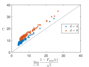
Figure 1: Scatter plot of the $\sqrt{\epsilon}$ coefficient in the expansion of $F_{\min}(\epsilon)$ inferred via SDP against the quantity $C$ in Thm. 2, which is an upper bound on the $\sqrt{\epsilon}$ coefficient. Each data point corresponds to a set of $d$ Haar random input states. A gray line with slope $m=1$ is included to aid the comparison.

VII Symmetric POVM input states

In this section, we prove lower and upper bounds on the process fidelity for a set of $N$ input states whose one-dimensional projectors form a symmetric positive operator-valued measure (POVM). Such sets are also referred to as equiangular tight frames Sustik2007 . We show that for such sets of input states, $F_{\mathrm{min}}$ is bounded by a linear function of the errors $\epsilon_{k}$. Our motivation for studying symmetric POVM input states is that they are in a sense maximally spread out in the Hilbert space $\mathcal{H}$, and are therefore good candidates for yielding the tightest possible bounds for a given $N$.

The set of input states forms a symmetric POVM if its states have constant pairwise overlap and the sum of the input projectors is proportional to the identity. That is, the input states satisfy that for some constant $c\geq 0$ and for all $k\not=k^{\prime}$

$$\absolutevalue{\bra{\psi_{k}}\ket{\psi_{k^{\prime}}}}^{2} =c,$$ (11)

$$\frac{d}{N}\sum_{k}\ket{\psi_{k}}\bra{\psi_{k}} =I,$$ (12)

where the factor $\frac{d}{N}$ is determined by matching the traces of the two sides of the identity. By squaring Eq. 12 and taking the trace, the constant in Eq. 11 is found to be

$$c=\frac{N-d}{d(N-1)}.$$ (13)

Conventionally, a POVM consists of a family of positive semidefinite hermitian operators summing to the identity. We slightly abused the terminology in referring to the set of input states as a POVM. The conventional POVM formed from the input states satisfying Eqs. 11 and 12 consists of the operators $\frac{d}{N}\hat{\psi}_{k}$. If the set of input states forms a symmetric POVM, then the input states are spanning. If $N>d$, the graph $G$ defined at the beginning of Sec. V is a complete graph. When $N=d^{2}$, the input projectors $\hat{\psi}_{k}$ span $B(\mathcal{H})$ and therefore form a symmetric informationally complete (SIC) POVM Renes2004 . At the other extreme, the smallest non-trivial symmetric POVM occurs when $N=d+1$, because for $N=d$ we have $c=0$ and $G$ is not connected. A set of $d+1$ states satisfying Eqs. 11 and 12 is called a simplex.

Whereas SIC POVMs are conjectured but not proven to exist in all dimensions Fuchs2017 , we give an explicit construction of a simplex. Let $\omega=\exp(2\pi i/(d+1))$ be a $(d+1)^{\mathrm{th}}$ root of unity. For $k\in\{0,1,..,d\}$, define

$$\ket{\psi_{k}}=\frac{1}{\sqrt{d}}\sum_{x=0}^{d-1}\omega^{kx}\ket{x}.$$ (14)

By direct calculation one can confirm that Eqs. 11 and 12 are satisfied.

Symmetric POVM input states have the nice property that $F_{\min}(\epsilon)$ is linear for constant $\epsilon_{k}=\epsilon$. An example is shown in Fig. 2, which shows $F_{\min}(\epsilon)$ when the set of input states is a simplex. The figure also shows $F_{\min}(\epsilon)$ for the set of input states $\{\ket{0},...,\ket{d-1},\ket{\psi_{tr}}\}$ from Ref. Reich2013 , which is not linear and has a more negative slope as $\epsilon$ goes to zero. This demonstrates that the simplex is a better choice of $d+1$ input states for obtaining lower bounds on the process fidelity. We conjecture that symmetric POVM states are optimal among all sets of $N$ input states in this regard.

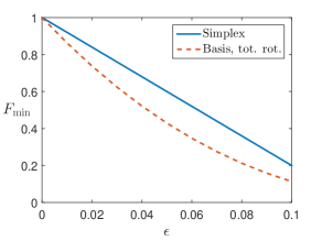
Figure 2: Plot of $F_{\mathrm{min}}(\epsilon)$ for two sets of input states in $d=8$ dimension. The solid curve is for the simplex, the dashed for the standard basis together with the totally rotated state defined in the text. Note that $F_{\mathrm{min}}$ is convex.

Our main result on the performance of symmetric POVMs is a general, linear bound on $F(\mathcal{E})$. After the proof we show that the lower bound is tight for $\epsilon_{k}=\epsilon$ constant.

Theorem 3.

Suppose that the set of input states with $N>d$ forms a symmetric POVM and let $\mathcal{E}$ be a CPTP map such that $1-u_{k}\geq\bra{\psi_{k}}\mathcal{E}(\hat{\psi}_{k})\ket{\psi_{k}}\geq 1-\epsilon_{k}$ for all $k$. Then

$$1-\bar{u}\geq F(\mathcal{E})\geq 1-\bigg{(}\frac{N-1}{N-d}\bigg{)}\,\bar{\epsilon},$$

where $\bar{\epsilon}$ and $\bar{u}$ are the means of the $\epsilon_{k}$ and $u_{k}$.

Proof.

We first prove that $F(\mathcal{E})\geq 1-(\frac{N-1}{N-d})\,\bar{\epsilon}=1-\frac{1}{dc}\bar{\epsilon}$, where $c$ is defined in Eq. 13. We apply the assumed bounds and Eq. 1 to obtain

$$(1-\epsilon_{k}) \leq\bra{\psi_{k}}\mathcal{E}(\hat{\psi}_{k})\ket{\psi_{k}}$$

$$=d\,\Tr(\hat{\psi}_{k}\Tr_{1}\left(\chi\,\left(\hat{\psi}_{k}^{\intercal}\otimes I\right)\right))$$

$$=d\,\Tr(\chi\,\left(\hat{\psi}_{k}^{\intercal}\otimes\hat{\psi}_{k}\right)).$$

Define $\Gamma=\sum_{k}\hat{\psi}_{k}^{\intercal}\otimes\hat{\psi}_{k}$. Summing the inequality just obtained over $k$ and dividing by $N$ gives $1-\bar{\epsilon}\leq\frac{d}{N}\mathrm{Tr}(\chi\Gamma)$, which is equivalent to

$$1-\frac{1}{dc}\bar{\epsilon}\leq 1-\frac{1}{dc}+\frac{1}{Nc}\mathrm{Tr}(\chi\Gamma).$$ (15)

The inequality to be proven follows once we show that $F(\mathcal{E})$ is bounded below by the right-hand-side. Since $F(\mathcal{E})=\mathrm{Tr}(\chi\hat{\phi})$, this is implied by

$$\mathrm{Tr}(\chi\hat{\phi})\geq 1-\frac{1}{dc}+\frac{1}{Nc}\mathrm{Tr}(\chi\Gamma).$$

After moving everything to the left-hand-side and defining

$$A=\hat{\phi}+\left(\frac{1}{dc}-1\right)\,I-\frac{1}{Nc}\Gamma,$$

we can see that the desired inequality is equivalent to $\mathrm{Tr}(\chi A)\geq 0$, and it suffices to prove that $A$ is positive semidefinite. For this purpose, we determine the spectral decomposition of $\Gamma$. We can write $\Gamma=BB^{{\dagger}}$ with $B$ given by

$$B=\sum_{k=1}^{N}\left(\ket{\psi_{k}^{*}}\otimes\ket{\psi_{k}}\right)\bra{k},$$

where $\ket{\psi_{k}^{*}}$ is the complex conjugate of $\ket{\psi_{k}}$ relative to the standard basis, and we used $\hat{\psi}_{k}^{*}=\hat{\psi}_{k}^{\intercal}$. $B$ is a matrix of dimension $d^{2}\times N$ and the spectrum of $BB^{{\dagger}}$ is the same as that of $B^{{\dagger}}B$, which is the $N\times N$ matrix whose $k,k^{\prime}$ entry is given by

$$\absolutevalue{\bra{\psi_{k}}\ket{\psi_{k^{\prime}}}}^{2}=((1-c)\delta_{kk^{\prime}}+c).$$

With respect to the basis consisting of the $\ket{k}$, this is a matrix whose diagonal entries are $1$ and whose off-diagonal entries are $c$. Such a matrix has two eigenvalues: the first is $(N-1)c+1=\frac{N}{d}$ corresponding to the eigenvector with constant entries, and the second is $(1-c)$ with multiplicity $N-1$. Accordingly, we can write

$$\Gamma=BB^{{\dagger}}=\frac{N}{d}\hat{\phi}^{\prime}+(1-c)\Pi,$$ (16)

where $\hat{\phi}^{\prime}$ is a rank-one projector and $\Pi$ is a rank $N-1$ projector orthogonal to $\hat{\phi}^{\prime}$. We determine that $\hat{\phi}^{\prime}=\hat{\phi}$ by verifying that $\ket{\phi}$ is an eigenstate of $\Gamma$ with eigenvalue $N/d$: From Eqs. 2 and 12,

$$\Gamma\ket{\phi} =\sum_{k}(\hat{\psi}_{k}^{\intercal}\otimes\hat{\psi}_{k})\ket{\phi}$$

$$=\sum_{k}(I\otimes\hat{\psi}_{k})\ket{\phi}$$

$$=\frac{N}{d}\ket{\phi}.$$

Let $\Pi_{\perp}=I-\hat{\phi}-\Pi$ be the projector onto the nullspace of $\Gamma$. We can now write $A$ as

$$A =\hat{\phi}+\left(\frac{1}{dc}-1\right)(\hat{\phi}+\Pi+\Pi_{\perp})$$

$$\hphantom{=\;}-\left(\frac{1}{dc}\hat{\phi}+\frac{1-c}{Nc}\,\Pi\right)$$

$$=\frac{d-1}{N-d}\,\Pi_{\perp},$$

since $\frac{1}{dc}-1=\frac{1-c}{Nc}=\frac{d-1}{N-d}$. Thus $A$ is positive semidefinite as claimed.

The proof that $F(\mathcal{E})\leq 1-\bar{u}$ follows the same strategy. Instead of Eq. 15, from the upper bound on the input state fidelities we derive $1-\bar{u}\geq\frac{d}{N}\mathrm{Tr}(\chi\Gamma)$. The inequality to be proven now is implied by $\mathrm{Tr}(\chi\hat{\phi})\leq\frac{d}{N}\mathrm{Tr}(\chi\Gamma)$, so it suffices to show that $\Tr(\chi A^{\prime})\leq 0$ with $A^{\prime}=\hat{\phi}-\frac{d}{N}\Gamma$. Applying Eq. 16 gives $A^{\prime}=-\frac{d}{N}(1-c)\Pi$, which is negative semidefinite since $c<1$. ∎

Numerical solutions indicate that the lower bound $F(\mathcal{E})\geq 1-(\frac{N-1}{N-d})\bar{\epsilon}$ of Thm. 3 is not tight. Determining $F_{\min}(\bm{\epsilon})$ for symmetric POVM input states and general $\epsilon_{k}$ remains an open problem. However, if $\epsilon_{k}=\epsilon$ for all $k$, then the lower bound is tight and achieved by the quantum channel

$$\mathcal{E}(\rho)=\left(1-p\right)\rho+p\frac{d}{N}\sum_{k}\hat{\psi}_{k}\rho\,\hat{\psi}_{k},$$ (17)

where $p=\frac{d(N-1)}{(d-1)(N-d)}\epsilon$. The Kraus operators for $\mathcal{E}$ are $\sqrt{1-p}\,I$ and $\sqrt{p\frac{d}{N}}\,\hat{\psi}_{k}$ for $k=1,\ldots,N$. We verify that $\mathcal{E}$ satisfies $\bra{\psi_{k}}\mathcal{E}(\hat{\psi}_{k})\ket{\psi_{k}}=1-\epsilon$ for all $k$ and $F(\mathcal{E})=1-(\frac{N-1}{N-d})\epsilon$:

$$\bra{\psi_{k}}\mathcal{E}(\hat{\psi}_{k})\ket{\psi_{k}} =(1-p)+p\frac{d}{N}\sum_{k^{\prime}}\absolutevalue{\bra{\psi_{k}}\ket{\psi_{k^{\prime}}}}^{4}$$

$$=(1-p)+p\frac{d}{N}\big{(}1+(N-1)c^{2}\big{)}$$

$$=1-p\frac{1}{N}\left(N-d-\frac{(N-d)^{2}}{d(N-1)}\right)$$

$$=1-p\frac{N-d}{dN(N-1)}\left(d(N-1)-(N-d)\right)$$

$$=1-p\frac{(N-d)(d-1)}{d(N-1)}$$

$$=1-\epsilon,$$

and

$$F(\mathcal{E}) =\bra{\phi}(I\otimes\mathcal{E})(\hat{\phi})\ket{\phi}$$

$$=(1-p)+p\frac{d}{N}\sum_{k}\absolutevalue{\bra{\phi}(I\otimes\hat{\psi}_{k})\ket{\phi}}^{2}$$

$$=(1-p)+p\frac{d}{N}\sum_{k}\frac{1}{d^{2}}$$

$$=1-p\frac{d-1}{d}$$

$$=1-\frac{N-1}{N-d}\epsilon.$$

When $N=d^{2}$, symmetric POVM input states form a SIC POVM and therefore also a 2-design Renes2004 . An argument similar to that in Ref. Nielsen2002 shows that the fidelity minimizing channel $\mathcal{E}$ defined in Eq. 17 is the depolarizing channel

$$\mathcal{E}(\rho)=(1-q)\rho+\frac{q}{d}I,$$

with $q=\frac{d}{d-1}\epsilon$. For the simplex, when $N=d+1$, the fidelity minimizing channel is in general more difficult to interpret. For the case of $d=2$ and with the explicit simplex states given in Eq. 14,

$$\mathcal{E}(\rho)=(1-2\epsilon)\rho+\epsilon(\sigma_{x}\rho\sigma_{x}+\sigma_{y}\rho\sigma_{y}),$$

where the $\sigma_{u}$ are the standard Pauli matrices. As can be seen, $\mathcal{E}$ is a sum of the $x$ and $y$ dephasing channels. In a Bloch-sphere-deformation picture, the effect is to maximize contraction parallel to the $z$-axis while keeping contraction parallel to the other axes fixed. The $z$-axis contraction is limited by the “no pancake theorem” Blume-Kohout2010 , which states that there is no quantum channel that projects the Bloch sphere onto the $x-y$ plane.

VIII Comparison to Hofmann bounds

Consider $N=d+1$ with $d=2^{n}$, where the state space is that of $n$ qubits. The set of simplex input states of Eq. 14 can be used in an efficient experimental procedure for bounding the fidelity of a process. These input states factor according to

$$\ket{\psi_{k}}=\bigotimes_{j=1}^{n}\frac{1}{\sqrt{2}}(\ket{0}+e^{i\pi k\frac{2^{n+1-j}}{d+1}}\ket{1}),$$

and can therefore be prepared with one-qubit Hadamard gates and rotations about the $z$-axis. If the measured state fidelities satisfy $\bra{\psi_{k}}\mathcal{E}(\hat{\psi}_{k})\ket{\psi_{k}}=1-\epsilon_{k}$, then according to Thm. 3 the process fidelity is bounded by

$$1-d\,\bar{\epsilon}\leq F(\mathcal{E})\leq 1-\bar{\epsilon}.$$ (18)

We compare these bounds to those given by Hofmann Hofmann2005 , which require as input states the members of two mutually unbiased bases (MUBs). A particular pair of such bases consists of the computational basis $\{\ket{x}\}$ and its Fourier transform $\{\ket{f_{x}}\}$ given by

$$\ket{f_{x}}=\frac{1}{\sqrt{d}}\sum_{y}e^{2\pi ixy/d}\ket{y}.$$

Thus, the Hofmann bounds require $2d$ input states, a quadratic improvement over full process tomography in the number of states needed to probe the fidelity of a process. The bounds are determined by the two classical fidelities

$$F_{1} =\frac{1}{d}\sum_{x}\bra{x}\mathcal{E}(\hat{x})\ket{x},$$

$$F_{2} =\frac{1}{d}\sum_{x}\bra{f_{x}}\mathcal{E}(\hat{f}_{x})\ket{f_{x}},$$

in terms of which they are given by

$$F_{1}+F_{2}-1\leq F(\mathcal{E})\leq\mathrm{min}\{F_{1},F_{2}\}.$$ (19)

Suppose that the fidelities for the input states used to apply the Hofmann bounds are $1-\epsilon_{k}$. Then $F_{1}+F_{2}-1=1-2\bar{\epsilon}$ and if $\epsilon_{k}=\epsilon$ is constant, $\mathrm{min}\{F_{1},F_{2}\}=1-\bar{\epsilon}$. For comparison, according to Thm. 3, a symmetric POVM with $N=2d$ yields lower and upper bounds of $1-(\frac{2d-1}{d})\bar{\epsilon}$ and $1-\bar{\epsilon}$. Assuming identical average errors, the lower bound is slightly tighter. The set of simplex input states consist of $d+1$ states, further reducing the number of input states by a factor approaching two. Because fewer input states are used, the bounds obtained with the simplex are looser than the Hofmann bounds. However, the improvement obtained from the Hofmann bounds depends on the particular process $\mathcal{E}$. For instance, if the system is subject to an error channel that is a depolarizing channel $\mathcal{D}(\rho)=(1-p)\rho+\frac{p}{d}I,$ with $\bra{\psi_{k}}\mathcal{D}(\hat{\psi}_{k})\ket{\psi_{k}}=1-\epsilon$, then for the simplex input states one finds that $F_{1}=F_{2}=1-\epsilon$ and so the Hofmann bounds are

$$1-2\epsilon\leq F(\mathcal{D})\leq 1-\epsilon.$$

The width of the interval between the lower and upper Hofmann bounds is smaller than that of Eq. 18 by a factor of $d-1$, so the advantage gained from using more input states grows linearly with the dimension. However, if the system encounters errors described by the process in Eq. 17, the classical fidelities are $F_{1}=1-d\epsilon$ and $F_{2}=1-\frac{d+1}{3}\epsilon$ (see appendix), giving the bounds

$$1-\Big{(}\frac{4d+1}{3}\Big{)}\epsilon\leq F(\mathcal{E})\leq 1-d\,\epsilon.$$ (20)

In this case the Hofmann bounds are tighter than the bounds in Eq. 18 by a factor approaching three for large dimensions. Interestingly, for the process given by Eq. 17, the upper bound obtained from Eq. 19 and the lower bound from Eq. 18 coincide. So for this particular channel, the classical fidelities for the Hoffman input states together with the average fidelity for the simplex input states determine the process fidelity exactly.

IX Conclusion

We have characterized sets of pure input states that identify unitary processes, and determined that the minimum number of states required is equal to the Hilbert space dimension $d$. We obtained a lower bound on $F(\mathcal{E})$ for small $\epsilon$ of the form $1-C\sqrt{\epsilon}-O(\epsilon)$ (Thm. 2). We have also proven bounds on $F(\mathcal{E})$ for symmetric POVM input states and shown that the lower bound is achieved for constant $\epsilon_{k}=\epsilon$. When $N=2d$, these bounds are slightly tighter than the Hofmann bounds obtained from a set of input states consisting of two MUBs. The smallest set of symmetric POVM input states which identifies unitaries is the simplex, with $N=d+1$. For qubit systems where $d=2^{n}$, simplex input states can be prepared with a circuit containing only Hadamard gates and individual $z$-axis rotations. However, the bounds obtained are in general much looser than the Hofmann bounds.

There are a number of open problems to be investigated. As noted, the bound given by Thm. 2 is not tight. Is there a tight bound expressed analytically in terms of the input states? What property of the input states determines the vanishing of the $O(\sqrt{\epsilon})$ term? Another open question is to find $F_{\min}(\bm{\epsilon})$ and the fidelity minimizing channel for symmetric POVM input states and arbitrary $\bm{\epsilon}$. A general problem is to determine, given $N$ and $\bar{\epsilon}$ or $\max_{k}\epsilon_{k}$, the maximum of $F_{\min}$ over all sets of input states of size $N$. Instead of the maximum $F_{\min}$ one can seek the minimum $F_{\max}$ or $F_{\max}-F_{\min}$. We conjecture that symmetric POVM states are optimal among all sets of $N$ input states, but numerical evidence suggests that symmetric POVMs do not exist for many $N$ with $d+1<N<d^{2}$ Tropp2005 ; Sustik2007 ; Fickus2015 . Finally, we observed that a set of input states containing both two MUBs and the simplex states determined $F(\mathcal{E})$ for the channel Eq. 17. This suggests the question of characterizing sets of input states and $\bm{\epsilon}$ that together determine the process fidelity exactly.

Appendix A Equivalence of UIC and graph connectivity

Proposition 3.

For a set of pure states $\{\ket{\psi_{k}}\}$, let $G=(V,E)$ be the graph with $V=\{1,\ldots,k\}$ and $E=\{(k,k^{\prime}):\bra{\psi_{k}}\ket{\psi_{k^{\prime}}}\neq 0\}$. The following two conditions are equivalent:

1. If $U\in U(d)$ and $[U,\hat{\psi}_{k}]=0$ for all $k$, then $U\propto I$

2. The $\ket{\psi_{k}}$ span $\mathcal{H}$ and the graph $G$ is connected.

Proof.

(1$\implies$2) This direction is essentially the same as the only-if part of Thm. 1. We prove the contrapositive. Suppose first that the states $\ket{\psi_{k}}$ do not span $\mathcal{H}$. Let $S$ be the span of $\{\ket{\psi_{k}}\}$, and $S^{\perp}$ the orthogonal complement of $S$. Then $U=I_{S}\oplus iI_{S^{\perp}}$ commutes with all $\hat{\psi}_{k}$ but is not proportional to the identity. Next, suppose that $G$ is disconnected. Let $S$ be the span of the states $\ket{\psi_{k}}$ in a connected component of $G$. Then $S\not=0$ and $S^{\perp}\not=0$, and again $U=I_{S}\oplus iI_{S^{\perp}}$ commutes with all $\hat{\psi}_{k}$ but is not proportional to the identity.

(2$\implies$1) Suppose that $U$ commutes with all $\hat{\psi}_{k}$. From $U\ket{\psi_{k}}\bra{\psi_{k}}=\ket{\psi_{k}}\bra{\psi_{k}}U$ it follows that $U\ket{\psi_{k}}=\omega_{k}\ket{\psi_{k}}$ with $\omega_{k}=\bra{\psi_{k}}U\ket{\psi_{k}}$. Therefore, $\innerproduct{\psi_{k^{\prime}}}{\psi_{k}}=\bra{\psi_{k^{\prime}}}U^{\dagger}U\ket{\psi_{k}}=\omega_{k^{\prime}}^{*}\omega_{k}\innerproduct{\psi_{k^{\prime}}}{\psi_{k}}$. If $k$ and $k^{\prime}$ are adjacent in $G$, we can divide both sides by $\innerproduct{\psi_{k^{\prime}}}{\psi_{k}}$ and conclude that $\omega_{k}=\omega_{k^{\prime}}$. Since $G$ is connected, all $\omega_{k}$ are equal, and since the states $\ket{\psi_{k}}$ span $\mathcal{H}$, it follows that $U$ is proportional to the identity . ∎

Appendix B Proof of Thm. 2

Suppose that the family of input states $\{\ket{\psi_{k}}\}_{k=1}^{N}$ spans $\mathcal{H}$, the graph $G=(V,E)$ defined by $V=\{1,\ldots,k\}$ and $E=\{(k,k^{\prime}):\bra{\psi_{k}}\ket{\psi_{k^{\prime}}}\neq 0\}$ is connected, and for all $k$ the process $\mathcal{E}$ satisfies

$$\quad\bra{\psi_{k}}\mathcal{E}(\hat{\psi}_{k})\ket{\psi_{k}}\geq 1-\epsilon.$$ (21)

By dilation we can express $\mathcal{E}$ as

$$\mathcal{E}(\hat{\psi}_{k})=\mathrm{Tr}_{B}(U(\hat{\psi}_{k}\otimes\ket{0}\bra{0})U^{{\dagger}}),$$

where $U$ is unitary and we introduced an ancillary system with initial state $\ket{0}$. We label the original input system by $A$, the ancillary system by $B$ and disambiguate kets and operators with label subscripts and bras with label presuperscripts, when necessary. The state $U\ket{\psi_{k}}\ket{0}$ can be written as

$$U\ket{\psi_{k}}\ket{0}=a_{k}\ket{\psi_{k}}_{A}\ket{e_{k}}_{B}+b_{k}\ket{s_{k}}_{AB},$$ (22)

where $\ket{e_{k}}$ is a normalized ancilla state, and $\ket{s_{k}}_{AB}$ satisfies ${}^{A}\!\!\bra{\psi_{k}}{}\ket{s_{k}}_{AB}=0$, and $a_{k}$ and $b_{k}$ are non-negative. The coefficients and states can be determined from the identity $a_{k}\ket{e_{k}}_{B}={}^{A}\!\!\bra{\psi_{k}}U\ket{\psi_{k}}_{A}\ket{0}_{B}$. Eq. 21 implies that $a_{k}\geq\sqrt{1-\epsilon}$ and therefore $b_{k}\leq\sqrt{\epsilon}$. Applying Eq. 22 for indices $k$ and $k^{\prime}$ gives

$$\bra{\psi_{k^{\prime}}}\ket{\psi_{k}} =\bra{0}\bra{\psi_{k^{\prime}}}U^{\dagger}U\ket{\psi_{k}}\ket{0}$$

$$=a_{k^{\prime}}a_{k}\bra{\psi_{k^{\prime}}}\ket{\psi_{k}}\bra{e_{k^{\prime}}}\ket{e_{k}}$$

$$\hphantom{=\;}+b_{k^{\prime}}a_{k}\bra{s_{k^{\prime}}}\,\ket{\psi_{k}}\ket{e_{k}}+a_{k^{\prime}}b_{k}\bra{\psi_{k^{\prime}}}\bra{e_{k^{\prime}}}\,\ket{s_{k}}$$

$$\hphantom{=\;}+O(\epsilon).$$

Let $\alpha_{k^{\prime}k}=b_{k^{\prime}}a_{k}\bra{s_{k^{\prime}}}\,\ket{\psi_{k}}\ket{e_{k}}+a_{k^{\prime}}b_{k}\bra{\psi_{k^{\prime}}}\bra{e_{k^{\prime}}}\,\ket{s_{k}}$. Then $|\alpha_{k^{\prime}k}|\leq 2\sqrt{\epsilon}$, and since $a_{k^{\prime}}a_{k}=1-O(\epsilon)$, we have

$$\bra{\psi_{k^{\prime}}}\ket{\psi_{k}}=\bra{\psi_{k^{\prime}}}\ket{\psi_{k}}\bra{e_{k^{\prime}}}\ket{e_{k}}+\alpha_{k^{\prime}k}+O(\epsilon).$$ (23)

If $k$ and $k^{\prime}$ are adjacent in $G$ we can divide both sides of Eq. 23 by $\bra{\psi_{k^{\prime}}}\ket{\psi_{k}}$, and obtain

$$\bra{e_{k^{\prime}}}\ket{e_{k}}=1-\frac{\alpha_{k^{\prime}k}}{\bra{\psi_{k^{\prime}}}\ket{\psi_{k}}}+O(\epsilon).$$

If $k$ and $k^{\prime}$ are not adjacent, there is a path $P$ from $k$ to $k^{\prime}$, and the above equation applies for each edge along the path. We make repeated use of the following fact: if $\innerproduct{b}{a}=1-\beta_{1}$ and $\innerproduct{c}{b}=1-\beta_{2}$, for $\beta_{1}$,$\beta_{2}\in\mathbb{C}$, then $\innerproduct{c}{a}=1-\beta$, with $\absolutevalue{\beta}\leq(\sqrt{\absolutevalue{\beta_{1}}}+\sqrt{\absolutevalue{\beta_{2}}})^{2}$, to leading order in $\absolutevalue{\beta_{1}}$,$\absolutevalue{\beta_{2}}$. This can be verified by expanding $\bra{c}\ket{a}=\bra{c}\left(\ket{b}\bra{b}+\Pi\right)\ket{a}$ with $\Pi$ the projector onto the orthogonal complement of $\ket{b}$. We conclude that

$$\innerproduct{e_{k^{\prime}}}{e_{k}}=1-\gamma_{kk^{\prime}}+O(\epsilon),$$ (24)

for complex $\gamma_{kk^{\prime}}$ satisfying

$$\absolutevalue{\gamma_{kk^{\prime}}}\leq 2\sqrt{\epsilon}\,\bigg{(}\sum_{(i,j)\in P}\absolutevalue{\innerproduct{\psi_{i}}{\psi_{j}}}^{-1/2}\bigg{)}^{2}.$$

Because this is true for any path from $k$ to $k^{\prime}$, we can choose the path such that the above sum is minimized. Therefore,

$$\absolutevalue{\gamma_{kk^{\prime}}}\leq 2\sqrt{\epsilon}\,W_{kk^{\prime}}^{2}$$ (25)

where $W_{kk^{\prime}}$ is defined by Eq. 10.

To compute the process fidelity we add an additional system $C$ and start with $AC$ in the maximally entangled state $\ket{\phi}_{AC}=\frac{1}{\sqrt{d}}\sum_{x}\ket{x}_{A}\ket{x}_{C}$. The process fidelity is then given by

$$F(\mathcal{E})=\Tr_{B}\bra{\phi}_{AC}U_{AB}\ket{\phi}_{AC}\ket{0}_{B}\bra{0}_{B}\bra{\phi}_{AC}U_{AB}^{\dagger}\ket{\phi}_{AC}.$$ (26)

By reordering if necessary, we can assume that $\{\ket{\psi_{k}}\}_{k=1}^{d}$ is a basis. There exists a (non-orthogonal and un-normalized) dual basis $\{|\widetilde{\psi}_{k}\rangle\}_{k=1}^{d}$, satisfying $\bra*{\widetilde{\psi}_{k}}\ket*{\psi_{k^{\prime}}}=\delta_{kk^{\prime}}$ for $1\leq k,k^{\prime}\leq d$. For the remainder of this proof, indices $k,k^{\prime}$ are in $\{1,\ldots,d\}$ by default. The computational basis states can be expanded as

$$\ket{x}=\sum_{k}\bra*{\widetilde{\psi}_{k}}\ket*{x}\ket{\psi_{k}}.$$

Expanding $\ket{\phi}_{AB}$ in terms of the computational basis and invoking Eq. 22 gives

$$\begin{split}U_{AB}\ket{\phi}_{AC}\ket{0}_{B}=\frac{1}{\sqrt{d}}\sum_{x}\sum_{k}\bra*{\widetilde{\psi}_{k}}\ket*{x}U_{AB}\ket{\psi_{k}}_{A}\ket{0}_{B}\ket{x}_{C}\\ =\frac{1}{\sqrt{d}}\sum_{x}\sum_{k}\bra*{\widetilde{\psi}_{k}}\ket*{x}\big{(}a_{k}\ket{\psi_{k}}_{A}\ket{e_{k}}_{B}+b_{k}\ket{s_{k}}_{AB}\big{)}\ket{x}_{C}.\end{split}$$

Applying $\bra{\phi}_{AC}$ on the left gives

$$\begin{split}\frac{1}{d}&\sum_{x}\sum_{k}\innerproduct*{\widetilde{\psi}_{k}}{x}\big{(}a_{k}\innerproduct{x}{\psi_{k}}\ket{e_{k}}_{B}+b_{k}{}^{A}\!\!\bra*{x}{\!\!}\ket*{s_{k}}_{AB}\big{)}\\ &=\frac{1}{d}\sum_{k}\big{(}a_{k}\ket{e_{k}}_{B}+b_{k}{}^{A}\!\!\bra*{\widetilde{\psi}_{k}}{\!\!}\ket*{s_{k}}_{AB}\big{)}.\end{split}$$

Substituting in Eq. 26 yields

$$F(\mathcal{E})=\frac{1}{d^{2}}\sum_{kk^{\prime}}\Big{\{}\innerproduct{e_{k^{\prime}}}{e_{k}}+b_{k}{}^{A}\!\!\bra*{\widetilde{\psi}_{k}}{}^{B}\!\!\bra{e_{k^{\prime}}}{\!\!}\ket{s_{k}}_{AB}+\\ b_{k}^{*}{}^{AB}\!\!\bra*{s_{k^{\prime}}}{\!\!}\ket*{\widetilde{\psi}_{k^{\prime}}}_{A}\ket{e_{k}}_{B}\Big{\}}+O(\epsilon).$$ (27)

To bound the magnitude of the sum involving $\innerproduct{e_{k^{\prime}}}{e_{k}}$, we apply Eqs. 24 and 25 to obtain

$$\begin{split}\absolutevalue{\frac{1}{d^{2}}\sum_{kk^{\prime}}\innerproduct{e_{k^{\prime}}}{e_{k}}}&=\absolutevalue{\frac{1}{d}+\frac{1}{d^{2}}\sum_{k\neq k^{\prime}}(1-\gamma_{kk^{\prime}})}\\ &=\absolutevalue{1-\frac{1}{d^{2}}\sum_{k\neq k^{\prime}}\gamma_{kk^{\prime}}}\\ &\geq 1-\frac{4\sqrt{\epsilon}}{d^{2}}\sum_{k>k^{\prime}}W_{kk^{\prime}}^{2}\end{split}$$

The terms ${}^{A}\!\!\bra*{\widetilde{\psi}_{k}}{}^{B}\!\!\bra*{e_{k^{\prime}}}{\!\!}\ket*{s_{k}}_{AB}$ and ${}^{AB}\!\!\bra*{s_{k^{\prime}}}{\!\!}\ket*{\psi_{k^{\prime}}}_{A}\ket*{e_{k}}_{B}$ are each bounded in magnitude by $\|\ket*{\widetilde{\psi}_{k}}\|$. To express this quantity in terms of the $\ket{\psi_{k}}$, define $C=\sum_{k}\ket{\psi_{k}}\bra{k}$. Since $\bra{k}C^{-1}\ket{\psi_{k^{\prime}}}=\bra{k}C^{-1}C\ket{k^{\prime}}=\delta_{kk^{\prime}}$ for all $k,k^{\prime}$, we have $\bra*{\widetilde{\psi}_{k}}=\bra{k}C^{-1}$ and $\|\ket*{\widetilde{\psi}_{k}}\|^{2}=\bra{k}C^{-1}(C^{-1})^{\dagger}\ket{k}=\bra{k}(C^{\dagger}C)^{-1}\ket{k}$. The matrix $M=C^{\dagger}C$ can be recognized as the Gram matrix for the states $\ket{\psi_{k}}$, in terms of which we can write

$$\|\ket*{\widetilde{\psi}_{k}}\|=\sqrt{(M^{-1})_{kk}}\,.$$

Substituting these bounds into the expression for the process fidelity in Eq. 27 gives

$$F(\mathcal{E})\geq 1-\frac{2}{d}\Big{(}\frac{2}{d}\sum_{k>k^{\prime}}W_{kk^{\prime}}^{2}+\sum_{k}\sqrt{(M^{-1})_{kk}}\Big{)}\sqrt{\epsilon}+O(\epsilon),$$

matching Thm. 2 in the main text. This lower bound can be generalized to the case of state dependent errors $\epsilon_{k}$. Working back through the derivation, it suffices to apply the following replacements to the expression for the lower bound:

$$W_{kk^{\prime}}^{2}\sqrt{\epsilon}\,\mapsto\,\min_{P\in\mathcal{P}_{kk^{\prime}}}\Bigg{(}\sum_{(i,j)\in P}\sqrt{\frac{\sqrt{\epsilon_{i}}+\sqrt{\epsilon_{j}}}{\absolutevalue{\innerproduct{\psi_{i}}{\psi_{j}}}}}\Bigg{)}^{2},$$

and

$$\sum_{k}\sqrt{(M^{-1})_{kk}}\sqrt{\epsilon}\,\mapsto\,\sum_{k}\sqrt{(M^{-1})_{kk}}\sqrt{\epsilon_{k}}.$$

Appendix C Derivation of Eq. 20

We set $N=d+1$. Given the channel

$$\begin{split}\mathcal{E}(\rho)&=(1-p)\rho+p\frac{d}{d+1}\sum_{k=0}^{d}\hat{\psi}_{k}\rho\,\hat{\psi}_{k},\\ p&=\frac{d^{2}}{d-1}\epsilon,\end{split}$$

and the expression for $\ket{\psi_{k}}$ in Eq. 14, we compute

$$\begin{split}\bra{x}\mathcal{E}(\hat{x})\ket{x}&=1-p+p\frac{d}{d+1}\sum_{k=0}^{d}\absolutevalue{\bra{x}\ket{\psi_{k}}}^{4}\\ &=1-d\,\epsilon.\end{split}$$

Therefore,

$$F_{1}=\frac{1}{d}\sum_{x}\bra{x}\mathcal{E}(\hat{x})\ket{x}=1-d\,\epsilon.$$

For the Fourier basis,

$$\bra{f_{x}}\mathcal{E}(\hat{f}_{x})\ket{f_{x}}=1-p+p\frac{d}{d+1}\sum_{k=0}^{d}\absolutevalue{\bra{f_{x}}\ket{\psi_{k}}}^{4},$$

where

$$\bra{f_{x}}\ket{\psi_{k}}=\frac{1}{d}\sum_{y=0}^{d-1}e^{2\pi iy(\frac{k}{d+1}-\frac{x}{d})}.$$

We compute

$$\sum_{k=0}^{d}\absolutevalue{\bra{f_{x}}\ket{\psi_{k}}}^{4}=\frac{d+1}{d^{4}}\sum_{(y_{1},y_{2},y_{3},y_{4})\in J}e^{-2\pi i(y_{1}-y_{2}+y_{3}-y_{4})x/d},$$

where $J$ consists of the tuples $(y_{1},\ldots,y_{4})$ satisfying $y_{1}-y_{2}+y_{3}-y_{4}=0\mod(d+1$) and $y_{i}\in\{0,\ldots,d-1\}$. For $m=0,d+1,-(d+1)$, let $J_{m}$ be the set of tuples $(y_{i})_{i=1}^{4}\in J$ such that $y_{1}-y_{2}+y_{3}-y_{4}=m$. Define $S_{m}(x)=\sum_{(y_{1},y_{2},y_{3},y_{4})\in J_{m}}e^{-2\pi i(y_{1}-y_{2}+y_{3}-y_{4})x/d}$. Then $\sum_{x}S_{\pm(d+1)}(x)=0$ and $\sum_{x}S_{0}(x)=d|J_{0}|$. For $|J_{0}|$ we get

$$|J_{0}| =\sum_{l=0}^{2(d-1)}\Big{|}\big{\{}(y_{1},y_{3}):$$

$$\hphantom{\sum_{l=0}^{2(d-1)}|\{}y_{1}+y_{3}=l\textrm{\ and\ }y_{1},y_{3}\in\{0,\ldots,d-1\}\big{\}}\Big{|}^{2}$$

$$=\sum_{l=0}^{d-1}(l+1)^{2}+\sum_{l=d}^{2(d-1)}(2(d-1)-l+1)^{2}$$

$$=d^{2}+2\sum_{l=1}^{d-1}l^{2}$$

$$=d^{2}+2\frac{1}{6}(d-1)(d)(2d-1).$$

We can now evaluate $F_{2}$.

$$F_{2} =\frac{1}{d}\sum_{x}\bra{f_{x}}\mathcal{E}(\hat{f}_{x})\ket{f_{x}}$$

$$=1-\left(\frac{d^{2}}{d-1}-\frac{d^{3}}{(d-1)(d+1)}\frac{d+1}{d^{4}}|J_{0}|\right)\epsilon$$

$$=1-\left(\frac{d^{2}}{d-1}-\frac{1}{d(d-1)}|J_{0}|\right)\epsilon$$

$$=1-\left(\frac{d^{2}}{d-1}-\frac{d}{d-1}-\frac{2d-1}{3}\right)\epsilon$$

$$=1-\frac{d+1}{3}\epsilon.$$

References

• (1) Isaac L Chuang and M A Nielsen. Prescription for experimental determination of the dynamics of a quantum black box. J. Mod. Opt., 44, 1997.
• (2) Holger F. Hofmann. Complementary classical fidelities as an efficient criterion for the evaluation of experimentally realized quantum operations. Phys. Rev. Lett., 94(160504), 2005.
• (3) Daniel M. Reich, Giulia Gualdi, and Christiane P. Koch. Minimum number of input states required for quantum gate characterization. Phys. Rev. A, 88(042309), 2013.
• (4) Jaromír Fiurášek and Michal Sedlák. Bounds on quantum process fidelity from minimum required number of quantum state fidelity measurements. Phys. Rev. A, 89(012323):1–6, 2014.
• (5) M. Micuda, M. Sedlák, I. Straka, M. Miková, M. Dusek, M. Jezek, and J. Fiurášek. Efficient experimental estimation of fidelity of linear optical quantum toffoli gate. Phys. Rev. Lett., 111(160407), 2013.
• (6) Michal Sedlák and Jaromír Fiurášek. Generalized Hofmann quantum process fidelity bounds for quantum filters. Phys. Rev. A, 93(4):1–10, 2016.
• (7) Koenraad Audenaert and Bart De Moor. Optimizing completely positive maps using semidefinite programming. Phys. Rev. A, 65(030302), 2002.
• (8) Michael A. Nielsen and Isacc L. Chuang. Quantum Computation and quantum information. Cambridge University Press, 2010.
• (9) M Choi. Completely Positive Linear Maps on Complex Matrices. Linear Algebr. Appl., 10, 1975.
• (10) A. Jamiolkowski. Linear transformations which preserve trace and positive semidefiniteness of operators. Reports Math. Phys., 3, 1972.
• (11) Michael A. Nielsen. A simple formula for the average gate fidelity of a quantum dynamical operation. Phys. Lett. A, 303, 2002.
• (12) Steven T. Flammia and Yi Kai Liu. Direct fidelity estimation from few Pauli measurements. Phys. Rev. Lett., 106(230501), 2011.
• (13) L. Vandenberghe and S. Boyd. Semidefinite Programming. SIAM Rev., 38, 1996.
• (14) Stephen Boyd and Lieven Vandenberghe. Convex Optimization. Cambridge University Press, 2004.
• (15) Inc. CVX Research. CVX: Matlab Software for Disciplined Convex Programming, version 2.1, 2012.
• (16) Charles H. Baldwin, Amir Kalev, and Ivan H. Deutsch. Quantum process tomography of unitary and near-unitary maps. Phys. Rev. A, 82(012110), 2014.
• (17) E. W. Dijkstra. A note on two problems in connexion with graphs. Numer. Math., 1, 1959.
• (18) Mátyás A. Sustik, Joel A. Tropp, Inderjit S. Dhillon, and Robert W. Heath. On the existence of equiangular tight frames. Linear Algebra Appl., 426, 2007.
• (19) Joseph M. Renes, Robin Blume-Kohout, A. J. Scott, and Carlton M. Caves. Symmetric informationally complete quantum measurements. J. Math. Phys., 45, 2004.
• (20) Christopher A. Fuchs, Michael C. Hoang, and Blake C. Stacey. The SIC Question: History and State of Play. pages 1–14, 2017.
• (21) Robin Blume-Kohout, Hui Khoon Ng, David Poulin, and Lorenza Viola. Information-preserving structures: A general framework for quantum zero-error information. Phys. Rev. A, 82(062306), 2010.
• (22) Joel A. Tropp, Inderjit S. Dhillon, Robert W. Heath, and Thomas Strohmer. Designing structured tight frames via an alternating projection method. IEEE Trans. Inf. Theory, 51, 2005.
• (23) Matthew Fickus and Dustin G. Mixon. Tables of the existence of equiangular tight frames. (i):1–21, 2015.