Interactive Reinforcement Learning with Dynamic Reuse of Prior Knowledge

Abstract

Reinforcement learning has enjoyed multiple successes in recent years. However, these successes typically require very large amounts of data before an agent achieves acceptable performance. This paper introduces a novel way of combating such requirements by leveraging existing (human or agent) knowledge. In particular, this paper uses demonstrations from agents and humans, allowing an untrained agent to quickly achieve high performance. We empirically compare with, and highlight the weakness of, HAT and CHAT, methods of transferring knowledge from a source agent/human to a target agent. This paper introduces an effective transfer approach, DRoP, combining the offline knowledge (demonstrations recorded before learning) with online confidence-based performance analysis. DRoP dynamically involves the demonstrator’s knowledge, integrating it into the reinforcement learning agent’s online learning loop to achieve efficient and robust learning.

1 Introduction

There have been increasingly successful applications of reinforcement learning Sutton and Barto (1998) methods in both virtual agents and physical robots. In complex domains, reinforcement learning (RL) often suffers from slow learning speeds, which is particularly detrimental when initial performance is critical. External knowledge may be leveraged by RL agents to improve learning — demonstrations have been shown to be useful for many types of agents’ learning Schaal (1997); Argall et al. (2009). To leverage demonstrations, one common method is transfer learning Taylor and Stone (2009), where one (source) agent is used to speed up learning in a second (target) agent. However, many existing transfer learning methods can provide limited help for complex tasks, since there are assumptions about the source and/or target agent’s internal representation, demonstration type, learning method, etc.

One approach is the Human Agent Transfer Taylor et al. (2011) (HAT) algorithm, which provided a framework where a source agent could demonstrate policy and a target agent could improve its performance over that policy. As refinement, a Confidence Human Agent Transfer Wang and Taylor (2017) algorithm was proposed by leveraging the confidence measurement on the policy. Notice that these methods are different from demonstration learning work like those discussed in Argall et al. (2009), as the target agent is learning to outperform demonstrators rather than just mimic them.

Probabilistic Policy Reuse Fernández and Veloso (2006) is another transfer learning approach. Like many other existing approaches, it assumes both the source and the target agents share the same internal representations and optimal demonstrations are required. But here we are focusing on improving learning performance without such assumptions. Existed policies could guide the learning direction as shown elsewhere Da Silva and Mackworth (2010); Brys et al. (2017), but well-formulated policies could be impracticable due to the complexity of the learning task or the cost of a domain expert’s time.

The target agent must handle multiple potential problems. First, the source agent may be suboptimal. Second, if multiple sources of prior knowledge are considered, they must be combined in a way to handle any inconsistancies. Third, the source agent typically cannot exhaustively demonstrate over the entire state space; some type of generalization must be used to handle unseen states. Fourth, the target agent may have a hard time balancing the usage of the prior knowledge and its own self-learned policy.

In this paper, we introduce DRoP (Dynamic Reuse of Prior), as a interactive method to assist Reinforcement Learning by addressing the above problems. DRoP uses temporal difference models to perform online confidence-based performence measurement on transferred knowledge. In addition, we have three action decision models to help the target agent balance between following the source advice and following its own learned knowledge. We evaluate DRoP using the domains of Cartpole and Mario, showing improvement over existing methods. Furthermore, through this novel online confidence-based measurement, DRoP is capable of distinguishing the quality of prior knowledge as well as leveraging demonstrations from multiple sources.

2 Background

This section presents a selection of relevant techniques.

2.1 Reinforcement Learning

By interacting with an environment, an RL agent can learn a policy to maximize an external reward. A Markov decision process is common formulation of the RL problem. In a Markov decision process, $A$ is a set of actions an agent can take and $S$ is a set of states. There are two (initially unknown) functions within this process: a transition function ($T:S\times A\mapsto S$) and a reward function ($R:S\times A\mapsto R$).

The goal of an RL agent is to maximize the expected reward — different RL algorithms have different ways of approaching this goal. For example, two popular RL algorithms that learn to estimate $Q$, the total long-term discounted reward, are SARSA Rummery and Niranjan (1994); Singh and Sutton (1996):

$$Q(s,a)\leftarrow Q(s,a)+\alpha[r+\gamma Q(s^{\prime},a^{\prime})-Q(s,a)]$$

and Q-learning Watkins and Dayan (1992):

$$Q(s,a)\leftarrow Q(s,a)+\alpha[r+\gamma\underset{a^{\prime}}{max}Q(s^{\prime},a^{\prime})-Q(s,a)]$$

2.2 Human Agent Transfer (HAT)

The goal of HAT Taylor et al. (2011) is to leverage demonstration from a source human or source agent, and then improve agents’ performance with RL. Rule transfer Taylor and Stone (2007) is used in HAT to remove the requirements on sharing the same internal algorithms representation between source and target agents. The following steps summarize HAT:

1. Learn a policy ($\pi:S\mapsto A$) from the source task.

2. Train a decision list upon the learned policy as “IF-ELSE” rules.

3. Bootstrap the target agent’s learning with trained decision rules. The target agent’s action is guided by rules under a decaying probability.

2.3 Confidence Human Agent Transfer (CHAT)

CHAT Wang and Taylor (2017) provides a method based on confidence — it leverages a source agent’s/human’s demonstration to improve its performance. CHAT measures the confidence in the source demonstration. Such offline confidence is used to predict how reliable the transferred knowledge is.

To assist RL, CHAT will leverage the source demonstrations to suggest an action in the agent’s current state, along with the calculated confidence. For example, CHAT would use Gaussian distribution to predict action from demonstration with a offline probability. If the calculated confidence is higher than a pre-tuned confidence threshold, the agent would consider the prior knowledge reliable and execute the suggested action.

3 Dynamic Reuse of Prior (DRoP)

This section introduces DRoP, which provides an online confidence-based performance analysis on knowledge transfer to assist reinforcement learning.

Prior research Chernova and Veloso (2007) used an offline confidence measure of demonstration data, similar to CHAT. In contrast, our approach performs online confidence-based analysis on the demonstrations during the target agent’s learning process. We introduce two types of temporal difference confidence measurements (section 3.1) and three types of action decision models (section 3.2), which differ by whether prior knowledge should be used in the agent’s current state.

DRoP follows a three step process:

1. Collect a demonstration dataset (state-action pairs).

2. Use supervised learning to train classifier on the demonstration data. Different types of classifiers could be applied in this step but this paper uses a fully connected neural network, and the confidence distribution is calculated through the softmax layer (calculation function in Section 3.1).

3. Algorithm 1 is used to assist an RL agent in the target task. The action decision models will determine whether to reuse the transferred knowledge trained in the previous step or to use the agent’s own Q-values. The online confidence model will be updated simultaneously, along with Q-values.

As learning goes on, there will be a balance between using the transferred knowledge and learned Q-values. Notice that we do not directly transfer or copy Q-values in the second step — the demonstrating agent can be different from the target agent (e.g., a human can teach an agent). The supervised learning step removes any requirements on the source demonstrator’s learning algorithm or representation.

Relative to other existing work, there are significant advantages of DRoP’s online confidence measurement: First, it removes the trial-and-error confidence threshold tuning process. Second, the target agent’s experience is used to measure confidence on demonstrations. DRoP performs the adaptive confidence-based performance analysis during the target agent’s learning. This online process can help guarantee the transfer knowledge is adapted to the target tasks. Third, there is no global reuse probability control, a parameter that is crucial in other knowledge reuse methods Wang and Taylor (2017); Taylor et al. (2011); Fernández and Veloso (2006) to avoid suboptimal asymptotic performance.

3.1 Temporal Difference Confidence Analysis

The online confidence metric is measured via a temporal difference (TD) approach. For each action source (learned Q function or prior knowledge), we build a TD model to measure the confidence-based performance via experience.

A confidence-based TD model is used to analyze the performance level of every action source with respect to every state. Once an action is taken, the confidence model will update the corresponding action source’s confidence value. Generally speaking, an RL agent should prefer the action source with higher confidence level: the expected reward would likely be higher by taking the action from that source.

Our dynamic TD confidence model updates as follows:

$$C(s)\leftarrow(1-F(\alpha))\times C(s)+F(\alpha)\times[G(r)+\gamma\times C(s^{\prime})]$$

where $\gamma$ is discount factor, $r$ is reward, and $\alpha$ is the update parameter. For continuous domains, function approximators such as tile coding Albus (1981) should be used — in this work we are using the same discretization approximator as $Q(s,a)$. We define two types of knowledge models, described next, although more are possible.

The confidence prior knowledge model is denoted by $CP(s)$. We have 2 update methods: Dynamic Rate Update (DRU) and Dynamic Confidence Update (DCU). For DRU, since DRoP uses a neural network for supervised classification in this paper, we define a dynamic updating rate based on a softmax (Bishop, 2006, pp. 206–209) layer’s classification distribution:

$$F(\alpha)=\alpha\times\max\big{\{}\frac{1}{\sum_{i}exp(\theta_{i}^{T}\cdot x)}\begin{bmatrix}exp(\theta_{1}^{T}\cdot x))\\ exp(\theta_{2}^{T}\cdot x))\\ ...\\ exp(\theta_{i}^{T}\cdot x))\end{bmatrix}\big{\}}$$

$\theta_{i}$ is the weight vector of the softmax layer and $x$ is the corresponding input. $\max\{\cdot\}$ in the above equation is the output confidence by the network. The update rate of $CP(s)$ will be bounded by the confidence of the corresponding classification. If the confidence is higher, the update rate will be larger (and vice versa). Besides, we use the original reward from the learning task: $G(r)=r$.

For DCU, we use a fixed update rate: $F(\alpha)=\alpha$, but the reward function leverages the confidence:

$$G(r)=\frac{r}{r\_max}\times\max\big{\{}\frac{1}{\sum_{i}exp(\theta_{i}^{T}\cdot x)}\begin{bmatrix}exp(\theta_{1}^{T}\cdot x))\\ exp(\theta_{2}^{T}\cdot x))\\ ...\\ exp(\theta_{i}^{T}\cdot x))\end{bmatrix}\big{\}}$$

In the above equation, $\frac{r}{r\_max}$ is a normalized reward ($r\_max$ denotes the maximum absolute reward value) and G(r) re-scales the reward using confidence distribution.

The confidence Q knowledge model is denoted by $CQ(s)$. $CQ(s)$ uses the same update methods with $F(\alpha)=\alpha$ and $G(r)=r$. $CQ(s)$ will be updated only if an action is provided through $Q(s,a)$.

3.2 Action Selection Methods

Given these TD-based confidence models, we introduce three action selection methods that balance an agent’s learned knowledge (CQ) with its prior knowledge (CP).

The hard decision model (HD) is greedy and attempts to maximize the current confidence expectation. Given current state $s$, action source $AS$ is selected as:

$$AS={\arg\max}[\{CQ(s),CP(s)\}],$$

where ties are broken randomly.

The soft decision model (SD) decides action source using probability distribution. To calculate the decision probability, we first normalize $CQ(s)$ and $CP(s)$: $R=\max\{|CQ(s)|,|PQ(s)|\}$, $rCQ=CQ(s)/R$, $rCP=CP(s)/R$. Then rescale $rCQ$ and $rCP$ using the hyperbolic tangent function (using $rCQ$ as example):

$$\tanh(rCQ)=\frac{e^{rCQ}-e^{-rCQ}}{e^{rCQ}+e^{-rCQ}}$$

The probability of selecting action source is defined as:

$$AS={\begin{cases}Q&P=\frac{\tanh\left({rCQ}\right)+1}{\tanh\left(rCP\right)+\tanh\left({rCQ}\right)+2}\\ Prior&P=\frac{\tanh\left({rCP}\right)+1}{\tanh\left(rCP\right)+\tanh\left({rCQ}\right)+2}\end{cases}}$$ (1)

If the confidence in the prior knowledge is high, the target agent would follow the prior with high probability. If the confidence in the prior knowledge is low, it might still be worth trying, but with lower probability. If the confidence in the prior knowledge is very low, the probability would then be almost zero.

The third model is the soft-hard-$\epsilon$ decision model (S-H-$\epsilon$), shown in Algorithm 2. This method takes advantage of the above two models by adding an $\epsilon$-greedy switch. That is to say, we have added an $\epsilon$-greedy policy over HD and SD: S-H-$\epsilon$ can both greedily exploit the confidence value and also perform probabilistic exploration. Notice that our method could also handle multiple-source demonstrations. By adding parallel prior models, the above $AS$ (in Equation 1) could be expanded into multiple cases:

$$AS={\begin{cases}{Prior}_{1}&P_{1}=\frac{\tanh({rCP}_{1})+1}{\underset{i}{\sum}\{\tanh({rCP}_{i})+1\}}\\ {Prior}_{2}&P_{2}=\frac{\tanh({rCP}_{2})+1}{\underset{i}{\sum}\{\tanh({rCP}_{i})+1\}}\\ \hskip 10.0pt...&\hskip 45.0pt...\\ {Prior}_{i}&P_{i}=\frac{\tanh({rCP}_{i})+1}{\underset{i}{\sum}\{\tanh({rCP}_{i})+1\}}\end{cases}}$$ (2)

Input: Prior knowledge model PM

1

2for each episode do

3       Initialize state $s$ to start state

4       for each step of an episode do

5            

6            if rand() $\leq\epsilon$ then

7                  %Exploration:

8                   $a\leftarrow$ random action

9            else

10                  %Action source (AS) selected via HD, SD, or S-H-$\epsilon$:

11                   $AS\leftarrow$ Action Decision Model

12                   if $AS==$ Prior Knowledge then

13                        $a\leftarrow$ action from Prior Knowledge

14                         Update CP

15                  else

16                        $a\leftarrow$ action that maximizes $Q$

17                         Update CQ

18                  

19            Execute action $a$

20             Observe new state $s^{\prime}$ and reward $r$

21             Update $Q$ (SARSA, Q-Learning, etc.);

22            

23      

24

Algorithm 1 DRoP: Target Learning Bootstrap

3.3 Optimum Convergence Property

Here we discuss the theoretical analysis of the convergence of DRoP. $\pi_{P}$ and $\pi_{Q}$ denote the policy of prior knowledge and learned Q knowledge, respectively. Given a fixed policy, the optimal convergence of TD iteration is proven, as was done by Sutton (1988). For the static prior knowledge policy, we have $\mathds{E}[CP(s)]=CP^{*}(s)$. For the Q knowledge, $CQ(s)=\sum\limits_{a}\pi_{Q}(a|s)q(s,a)$. Since $q(s,a)$ is updated independently (Line 1 of Algorithm 1) and the Q-learning’s convergence is guaranteed by Melo (2001), we also have $\mathds{E}[CQ(s)]=CQ^{*}(s)$ on the converged $\pi^{*}_{Q}$. We will then prove that whatever the quality of prior knowledge is, DRoP will not harm Q-learning’s asymptotic performance.

Proof.

Given state $s$, if $CP^{*}(s)\geq CQ^{*}(s)$, which means the optimal $\pi^{*}_{P}(s)$ is better than $\pi^{*}_{Q}(s)$, the proof is trivial because following prior knowledge would result in higher reward. On states where $CP^{*}(s)<CQ^{*}(s)$, according to Line 2 of Algorithm 2 the probability of using suboptimal action is $\epsilon\times\frac{\tanh\left({rCP}\right)+1}{\tanh\left(rCP\right)+\tanh\left({rCQ}\right)+2}<\epsilon$, which means the suboptimal action is under $\epsilon$-greedy control. ∎

We therefore conclude that DRoP should guarantee the learning optimum, and Q-learning’s convergence will not be harmed even if the prior knowledge contains suboptimal data.

Input: $CQ,CP,$ State $s$

1 $R=\max\{|CQ(s)|,|PQ(s)|\}$

2 $rCQ=CQ(s)/R$

3 $rCP=CP(s)/R$

4 if rand() $\leq\epsilon$ then

5      if rand() $\leq\frac{\tanh\left({rCQ}\right)+1}{\tanh\left(rCP\right)+\tanh\left({rCQ}\right)+2}$ then

6             $AS$ = Prior Knowledge

7      else

8             $AS$ = Q  Knowledge

9      

10else

11       $AS={\arg\max}[\{CQ(s),CP(s)\}]$

$\textnormal{{return}}\ AS$ %Action source

Algorithm 2 S-H-$\epsilon$ : Hard-Soft-$\epsilon$ Decision Model

4 Experiment Setup

This section details our experimental methodology.

4.1 Experiment Domains

We evaluate our method in two domains: Cartpole and Mario.

Cartpole is a classic control problem – balancing a light-weight pole hinged to a cart. Our Cartpole simulation is based on the open-source OpenAI Gym Brockman et al. (2016). This task has a continuous state space; the world state is represented as 4-tuple vector: position of the cart, angle of the pole, and their corresponding velocity variables. The system is controlled by applying a force of +1 or -1 to the cart. Cartpole’s reward function is designed as: $+1$ for every surviving step and $-500$ if the pole falls.

Mario is a benchmark domain Karakovskiy and Togelius (2012) based on Nintendo’s Mario Brothers. We train the Mario agent to score as many points as possible. To guarantee the diversity and complexity of tasks, our simulation world is randomly sampled from a group of one million worlds. The world state is represented as a 27-tuple vector, encoding the agent’s state/position information, surrounding blocks, and enemies Suay et al. (2016). There are $12\ (3\times 2\times 2)$ possible actions (move direction $\times$ jump button $\times$ Run/Fire button).

4.2 Methodology

DRoP can work with demonstrations collected from both humans and other agents. In our experiments, demonstrations are collected either from a human participant (one of the authors of this paper) via a simulation visualizer, or directly from an agent executing the task.

We use a “4-15-15-2” network (15 nodes in two hidden layers) network in Cartpole and a “27-50-50-12” network in Mario. To benchmark against CHAT, we use the same networks as the confidence models used by DRoP. To benchmark against HAT, J48 Quinlan (1993) is used to train decision rules. Our classifiers are trained using classification libraries provided by Weka 3.8 Witten and Frank (2005). For both CHAT and HAT, the self-decaying reuse probability control parameter $\Phi$ was tuned to be 0.999 in Cartpole and 0.9999 in Mario. Target agents in both Cartpole and Mario are using Q-learning algorithm. In Cartpole, we use $\alpha=0.2,\gamma=0.9,\epsilon=0.1$. In Mario, we use $\alpha=\frac{1}{10\times 32},\gamma=0.9,\epsilon=0.1$. These parameters are set to be consistent with previous research Wang and Taylor (2017); Brys et al. (2015) in these domains.

Experiments are evaluated in terms of learning curves, the jumpstart, the total reward, and the final reward. Jumpstart is defined as the initial performance improvement, compared to an RL agent with no prior knowledge. The total reward accumulates scores every 5 percent of the whole training time. Experiments are averaged over 10 learning trials and t-tests are performed to evaluate the significance. Error bars on the learning curves show the standard deviation.

5 Experimental Results

This section will present and discuss our main experimental results. We first show the improvement over existing knowledge reuse algorithms, HAT and CHAT, as well as baseline learning. Then we show DRoP is capable of leveraging different quality demonstrations from multiple sources. Finally we will evaluate how DRoP could be used for interactive RL by efficiently involving a human demonstrator in the loop.

5.1 Improvement over Baselines

In Cartpole, we first let a trained agent demonstrate 20 episodes (average number of steps: 821 $\pm$ 105) and record those state-action pairs. In Mario, we let a trained agent demonstrate 20 episodes (average reward: 1512 $\pm$ 217).

DRoP is then used with these demonstration datasets. As benchmarks, we run HAT and CHAT on the same datasets, and Q-learning is run without prior knowledge. Learning performance is compared in Table 1. DRoP with different models outperforms the baselines. The top two scores for each type of performance are underlined. DRoP with DRU and S-H-$\epsilon$ model has achieved the best learning result and further discussions in the next sections use this setting. Statistically significant ($p<10^{-4}$) improved scores in Table 1 are in bold. There is no significant difference ($p>0.05$) from CHAT and HAT, for the final reward of Mario.

To highlight the improvement, Figure 1 and 2 show the learning curves of DRoP using DRU method. All three action selection schemes of DRoP (DRU) outperform HAT, CHAT, and baseline learning, indicating that DRoP is most effective.

Method	Cartpole			Mario
	Jumpstart	Total Reward	Final Reward	jumpstart	Total Reward	Final Reward
Q-Learning	N/A	11653	951 $\pm$ 36	N/A	27141	1569 $\pm$ 51
HAT	225	16283	1349 $\pm$ 84	651	25223	1577 $\pm$ 49
CHAT	258	22692	1766 $\pm$ 68	1046	30144	1574 $\pm$ 46
DCU, H-D	298	29878	1994 $\pm$ 62	829	31021	1675 $\pm$ 59
DCU, S-D	301	33498	2085 $\pm$ 79	880	31436	1690 $\pm$ 62
DCU, S-H-$\epsilon$	308	35312	2383 $\pm$ 71	909	32108	1752 $\pm$ 55
DRU, H-D	334	29563	1989 $\pm$ 63	845	30644	1668 $\pm$ 41
DRU, S-D	305	38576	2111 $\pm$ 90	905	31690	1681 $\pm$ 44
DRU, S-H-$\epsilon$	303	35544	2411 $\pm$ 56	915	33022	1779 $\pm$ 61

Table 1: This table compares baselines (methods 1 to 3) with DRoP using different models (methods 4 to 9). Jumpstart, total reward, and final reward are shown. The top two scores of each column are underscored and significant improvements over Q-learning are bold.

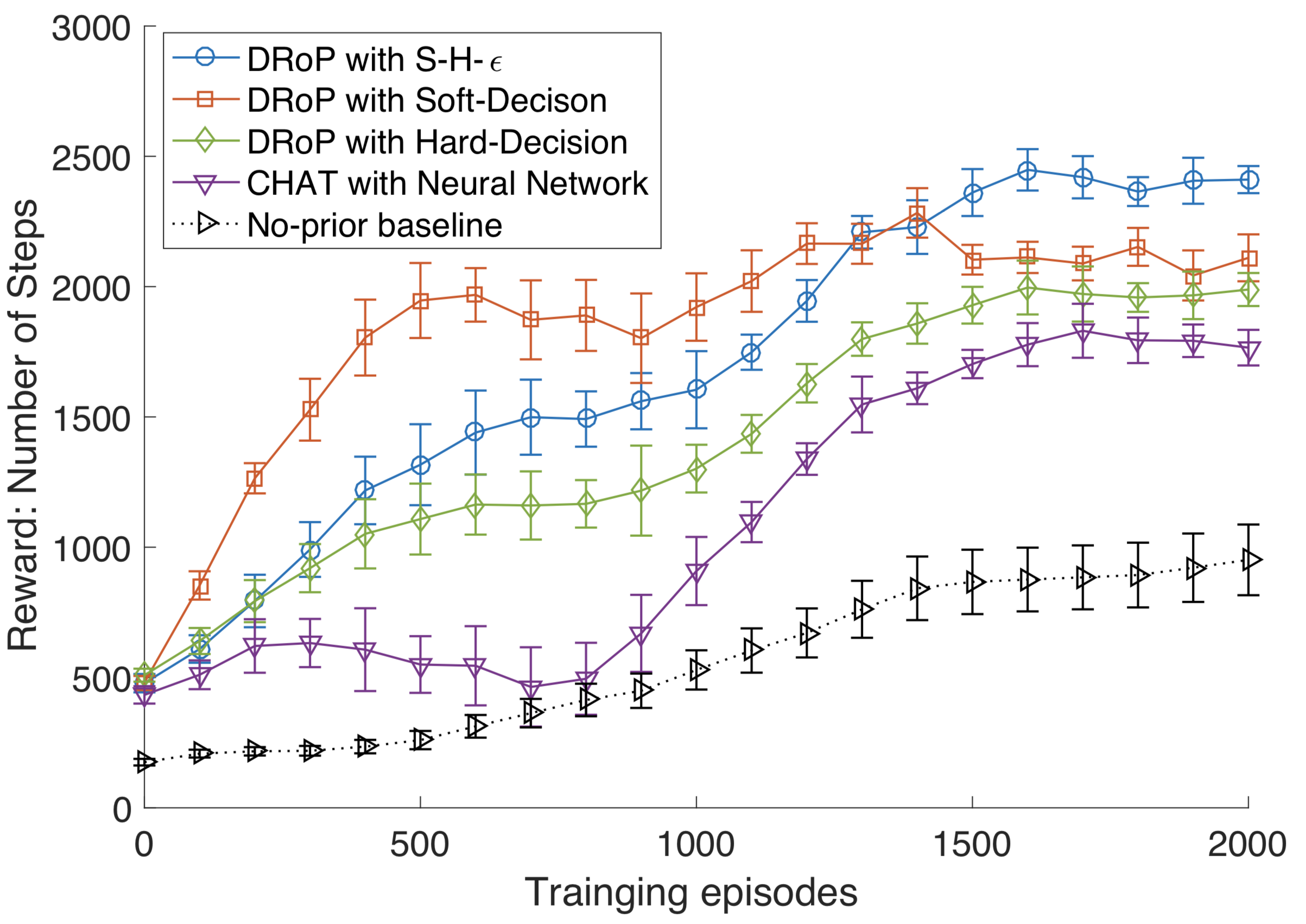
Figure 1: Cartpole learning curves

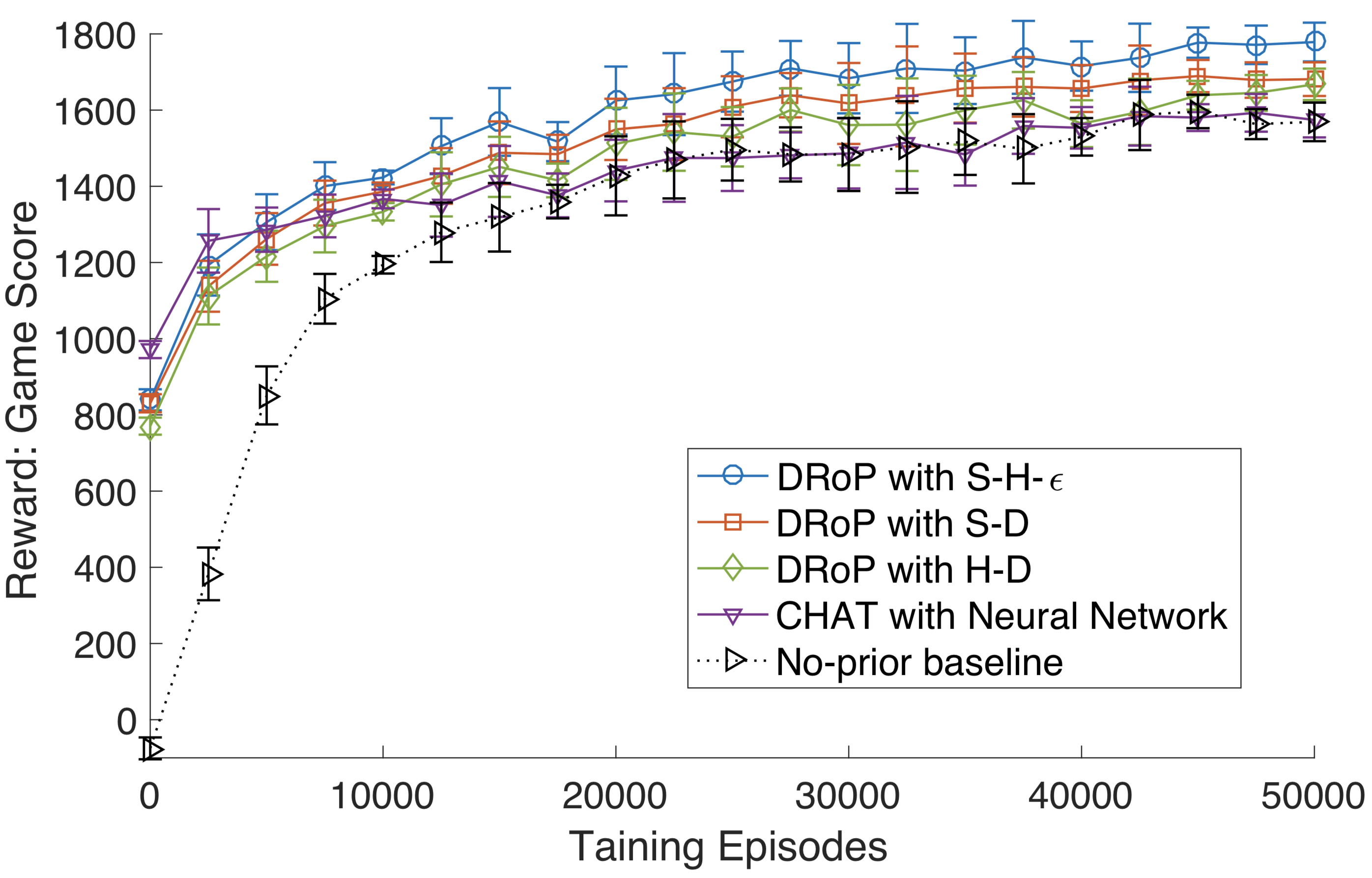
Figure 2: Mario learning curves

5.2 DRoPping Low-quality Demonstrations

We consider using suboptimal demonstrations to see how well the online confidence-based analysis mechanism can handle poor data without harming the optimal convergence. Here we have five different groups of demonstrations (recorded from different agents), ranging from completely random to high performing (shown in Tables 2 and 3).

We first evaluate our method individually with the five demonstration datasets. Cartpole results are shown in Table 2 and Mario results are shown in Table 3. As we can see, the quality of the demonstration does effect performance, and better demonstrations lead to better performance. However, what is more important is whether poor demonstrations hurt learning. If we look at the results of using randomly generated demonstrations, we find that even if the jumpstart is negative (i.e., the initial performance is hurt by using poor demonstrations), the final converged performance is almost the same as learning without the poor demonstrations. In addition, the converged reuse frequency (average percentage of actions using the prior knowledge) of random demonstration is almost zero, which means the DRoP agent has learned to ignore the poor demonstrations. As the demonstration quality goes higher (from L1 to L4), DRoP will reuse the prior knowledge with higher probability.

We evaluate the multiple-case model (Equation 2 by providing the above demonstrations simultaneously to DRoP and results are shown in Table 4. When low-quality demonstrations are mixed in the group, we see a decreased jumpstart from both CHAT and DRoP, relative to that seen in Table 2. In contrast, DRoP distinctly reuses the high-quality data more often and achieves better performance.

Demo Performance	Jump- start	Converged Performance	Converged Reuse Frequency
Q-Learning	N/A	951 $\pm$ 136	N/A
Rand: 15 $\pm$ 7	-5	942 $\pm$ 142	0.02 $\pm$ 0.01
L1: 217 $\pm$ 86	153	1453 $\pm$ 96	0.12 $\pm$ 0.03
L2: 435 $\pm$ 83	211	1765 $\pm$ 112	0.17 $\pm$ 0.04
L3: 613 $\pm$ 96	278	2080 $\pm$ 86	0.21 $\pm$ 0.02
L4: 821 $\pm$ 105	303	2411 $\pm$ 56	0.32 $\pm$ 0.03

Table 2: This table shows the performance of Q-learning and DRoP (DRU, S-H-$\epsilon$) upon 5 different levels of demonstrations in Cartpole.

Demo Performance	Jump- start	Converged Performance	Converged Reuse Frequency
Q-Learning	N/A	1569 $\pm$ 51	N/A
Rand: -245 $\pm$ 11	-52	1552 $\pm$ 72	0.01 $\pm$ 0.01
L1: 315 $\pm$ 183	336	1582 $\pm$ 67	0.08 $\pm$ 0.02
L2: 761 $\pm$ 195	512	1601 $\pm$ 73	0.15 $\pm$ 0.05
L3: 1102 $\pm$ 225	784	1695 $\pm$ 81	0.19 $\pm$ 0.03
L4: 1512 $\pm$ 217	906	1779 $\pm$ 61	0.28 $\pm$ 0.04

Table 3: This table shows the performance of Q-learning and DRoP (DRU, S-H-$\epsilon$) upon 5 different levels of demonstrations in Mario.

Method	Jumpstart	Converged Performance	Converged Reuse Frequency
CHAT	191	983 $\pm$ 151	0.05 $\pm$ 0.02
DRoP	253	2286 $\pm$ 91	Rand: 0.02 $\pm$ 0.01
			L1: 0.05 $\pm$ 0.01
			L2: 0.06 $\pm$ 0.02
			L3: 0.11 $\pm$ 0.03
			L4: 0.23 $\pm$ 0.02

Table 4: This table shows the performance of DRoP (DRU, S-H-$\epsilon$) and CHAT upon multiple sources of demonstrations in Cartpole.

5.3 DRoP-in Requests for Demonstrations

We have shown that DRoP is capable of analyzing the quality of demonstration. This section asks a different question — can DRoP use these confidence values to productively request additional demonstrations from a human or agent?

In Mario, we first recorded 20 episodes of demonstrations from an human expert with an average score of 1735. We then used DRoP to assist an RL agent’s learning. After a short period of training (1000 episodes), we then use the following steps to ask for additional demonstrations from the same human demonstrator over in the next 20 episodes:

1. Calculate average confidence of prior knowledge (i.e., $CP(s)$) at each step of the current episode:

   $$AveC=\frac{1}{steps}\times\underset{i}{\sum}CP(s_{i})$$

2. Use a sliding window of 10 $\times$ 10 to scan neighbourhood positions and calculate the average “$CP(s)$” within that sliding window.

3. If the averaged CP value is smaller than $AveC$, request a demonstration of 20 actions, starting at the current state.

4. Add the above recorded state-action pairs into the request demonstration dataset of DRoP.

The requested demonstration dataset is still recorded within 20 episodes, but the time spent actively demonstrating is reduced by 44%, relative to demonstrating for 20 episodes (shown in Table 5), because demonstrations are requested only when the agent’s confidence of prior knowledge is low. The time cost of demonstration collection is only 2% of the baseline training time, highlighting the efficincy of DRoP. We then compare it with the originally collected demonstration from the same human.

Figure 3 shows the performance comparison between the two demonstration datasets: 20 episodes of original human demonstrations and 20 episodes requested by DRoP. Notice that even though human’s demonstration performance is higher than the L4 dataset from the previous section, the actual jumpstart of the former is instead lower. This is potential evidence that a virtual agent could not “digest” the entire human demonstrator’s knowledge. In contrast, learning improvement from the extra demonstration requested by DRoP is higher. DRoP would request the demonstration from human only in states where the knowledge confidence is relatively low. Therefore, we know that the target agent truly needs these requested demonstrations. DRoP improved the overall learning effectiveness by requesting less, but critical, demonstration data.

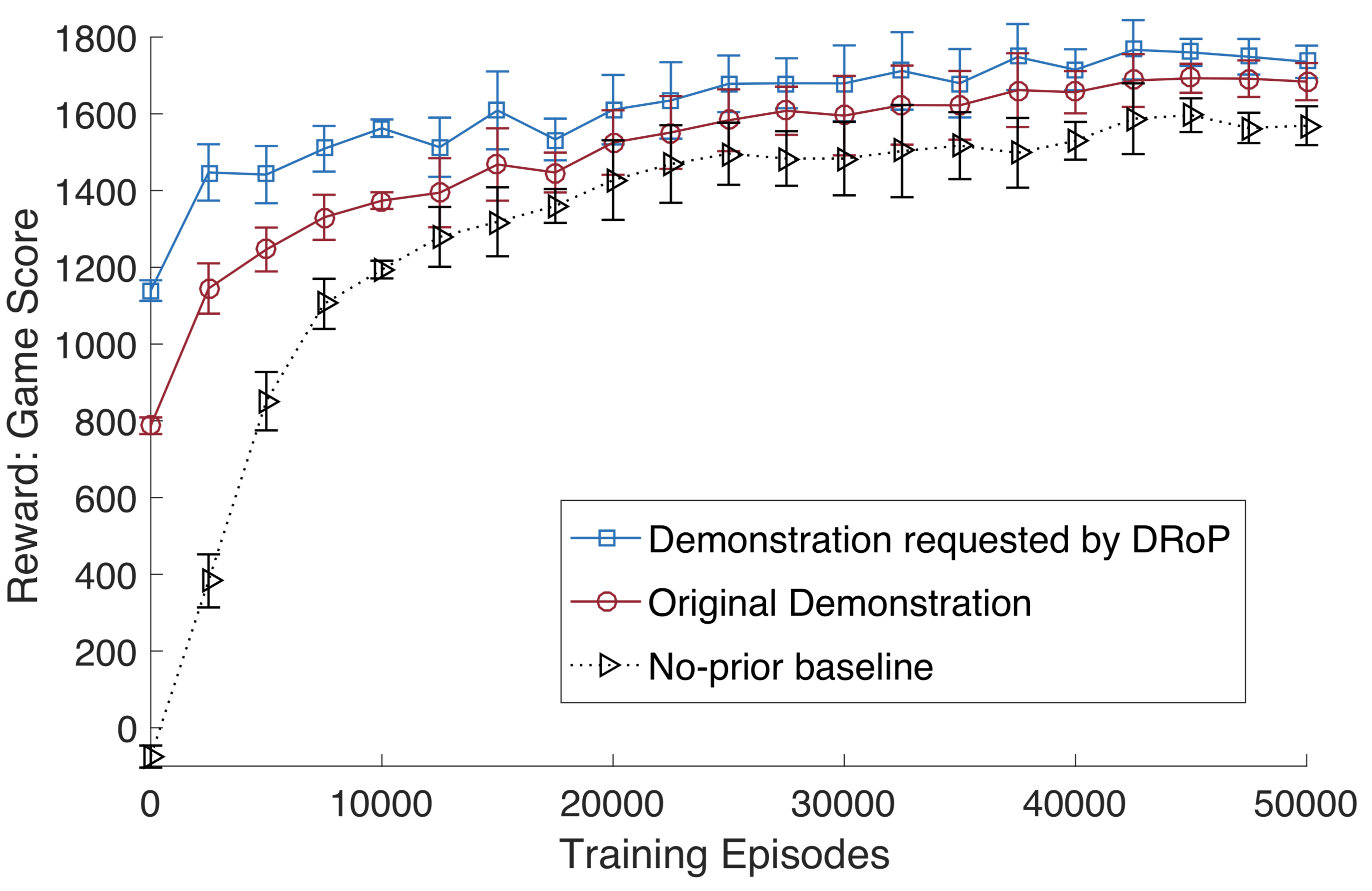
Figure 3: Mario learning curves using demonstration requested by DRoP and original demonstration from human expert.

Souce	Time Cost	Jumpstart	Converged Performance
Baseline	15325 s	N/A	951 $\pm$ 136
Original	623 s	862	1684 $\pm$ 49
Request	348 s	1214	1736 $\pm$ 42

Table 5: This table compares the original human demonstration and demonstration requested by DRoP (DRU, S-H-$\epsilon$) in Mario.

6 Conclusion and Future Work

This paper has introduced DRoP and evaluated it in two domains. This work shows that by integrating offline confidence with online temporal difference analysis, knowledge transfer from source agents or humans can be successfully achieved. DRoP outperformed both learning without prior knowledge and recent transfer methods.

DRoP’s confidence measurement is based on temporal difference (TD) models. Results suggest that such online confidence techniques can provide reasonable and reliable analysis of the quality of prior knowledge.

Two temporal difference methods and three action selection models are introduced in this work. It is shown that DRoP’s decision mechanism can leverage multiple sources of demonstrations. In our experimental domains, DRU with S-H-$\epsilon$ produced the best performance.

Results have shown that demonstrations requested by DRoP can significantly improve the RL agent’s learning process, leading to a more efficient collaboration between two very different types of knowledge entities: humans and virtual agents.

There are a number of interesting directions for future work, including the following. First, we will explore model-based demonstrations to see if any particular model structure could provide better confidence measurement than classification equally over all state-action pairs. Second, we will use DRoP to build a lifelong online learning system. Our current work could analyze and selectively reuse transferred static prior knowledge and the goal is to let the learning system automatically refine that knowledge model during learning.

References

- Albus [1981] JS Albus. Brains, behavior. & Robotics. Peterboro, NH: Byte Books, 1981.
- Argall et al. [2009] Brenna D Argall, Sonia Chernova, Manuela Veloso, and Brett Browning. A survey of robot learning from demonstration. Robotics and autonomous systems, 57(5):469–483, 2009.
- Bishop [2006] Christopher M Bishop. Pattern recognition. Machine Learning, 128:1–58, 2006.
- Brockman et al. [2016] Greg Brockman, Vicki Cheung, Ludwig Pettersson, Jonas Schneider, John Schulman, Jie Tang, and Wojciech Zaremba. Openai gym. arXiv preprint arXiv:1606.01540, 2016.
- Brys et al. [2015] Tim Brys, Anna Harutyunyan, Matthew E Taylor, and Ann Nowé. Policy transfer using reward shaping. In Proceedings of the 2015 International Conference on Autonomous Agents and Multiagent Systems, pages 181–188. International Foundation for Autonomous Agents and Multiagent Systems, 2015.
- Brys et al. [2017] Tim Brys, Anna Harutyunyan, Peter Vrancx, Ann Nowé, and Matthew E Taylor. Multi-objectivization and ensembles of shapings in reinforcement learning. Neurocomputing, 2017.
- Chernova and Veloso [2007] Sonia Chernova and Manuela Veloso. Confidence-based policy learning from demonstration using gaussian mixture models. In Proceedings of the 6th international joint conference on Autonomous agents and multiagent systems, page 233. ACM, 2007.
- Da Silva and Mackworth [2010] Bruno N Da Silva and Alan Mackworth. Using spatial hints to improve policy reuse in a reinforcement learning agent. In Proceedings of the 9th International Conference on Autonomous Agents and Multiagent Systems, pages 317–324. International Foundation for Autonomous Agents and Multiagent Systems, 2010.
- Fernández and Veloso [2006] Fernando Fernández and Manuela Veloso. Probabilistic policy reuse in a reinforcement learning agent. In Proceedings of the fifth international joint conference on Autonomous agents and multiagent systems, pages 720–727. ACM, 2006.
- Karakovskiy and Togelius [2012] Sergey Karakovskiy and Julian Togelius. The Mario AI benchmark and competitions. IEEE Transactions on Computational Intelligence and AI in Games, 4(1):55–67, 2012.
- Melo [2001] Francisco S Melo. Convergence of Q-learning: A simple proof. Institute Of Systems and Robotics, Tech. Rep, pages 1–4, 2001.
- Quinlan [1993] Ross Quinlan. C4.5: Programs for Machine Learning. Morgan Kaufmann Publishers, San Mateo, CA, 1993.
- Rummery and Niranjan [1994] Gavin A Rummery and Mahesan Niranjan. On-line Q-learning using connectionist systems. Technical report, CUED/F-INFENG/TR166, University of Cambridge, Engineering Dept., 1994.
- Schaal [1997] Stefan Schaal. Learning from demonstration. In Advances in neural information processing systems, pages 1040–1046, 1997.
- Singh and Sutton [1996] Satinder P Singh and Richard S Sutton. Reinforcement learning with replacing eligibility traces. Machine learning, 22(1-3):123–158, 1996.
- Suay et al. [2016] Halit Bener Suay, Tim Brys, Matthew E Taylor, and Sonia Chernova. Learning from demonstration for shaping through inverse reinforcement learning. In Proceedings of the 2016 International Conference on Autonomous Agents & Multiagent Systems, pages 429–437. International Foundation for Autonomous Agents and Multiagent Systems, 2016.
- Sutton and Barto [1998] Richard S Sutton and Andrew G Barto. Reinforcement learning: An introduction, volume 1. MIT press Cambridge, 1998.
- Sutton [1988] Richard S Sutton. Learning to predict by the methods of temporal differences. Machine learning, 3(1):9–44, 1988.
- Taylor and Stone [2007] Matthew E Taylor and Peter Stone. Cross-domain transfer for reinforcement learning. In Proceedings of the 24th international conference on Machine learning, pages 879–886. ACM, 2007.
- Taylor and Stone [2009] Matthew E. Taylor and Peter Stone. Transfer Learning for Reinforcement Learning Domains: A Survey. Journal of Machine Learning Research, 10(1):1633–1685, 2009.
- Taylor et al. [2011] Matthew E. Taylor, Halit Bener Suay, and Sonia Chernova. Integrating reinforcement learning with human demonstrations of varying ability. In Proceedings of the International Conference on Autonomous Agents and Multiagent Systems (AAMAS), May 2011.
- Wang and Taylor [2017] Zhaodong Wang and Matthew E. Taylor. Improving Reinforcement Learning with Confidence-Based Demonstrations. In Proceedings of the 26th International Conference on Artificial Intelligence (IJCAI), August 2017.
- Watkins and Dayan [1992] Christopher JCH Watkins and Peter Dayan. Q-learning. Machine learning, 8(3-4):279–292, 1992.
- Witten and Frank [2005] Ian H. Witten and Eibe Frank. Data Mining: Practical Machine Learning Tools and Techniques. Morgan Kaufmann, San Francisco, 2nd edition, 2005.