X-ray Absorption in Young Core-Collapse Supernova Remnants

Abstract

The material expelled by core-collapse supernova (SN) explosions absorbs X-rays from the central regions. We use SN models based on three-dimensional neutrino-driven explosions to estimate optical depths to the center of the explosion, compare different progenitor models, and investigate the effects of explosion asymmetries. The optical depths below 2 keV for progenitors with a remaining hydrogen envelope are expected to be high during the first century after the explosion due to photoabsorption. A typical optical depth is $100\,t_{4}^{-2}\,E^{-2}$, where $t_{4}$ is the time since the explosion in units of 10 000 days (${\sim}$27 years) and $E$ the energy in units of keV. Compton scattering dominates above 50 keV, but the scattering depth is lower and reaches unity already at ${\sim}$1000 days at 1 MeV. The optical depths are approximately an order of magnitude lower for hydrogen-stripped progenitors. The metallicity of the SN ejecta is much higher than in the interstellar medium, which enhances photoabsorption and makes absorption edges stronger. These results are applicable to young SN remnants in general, but we explore the effects on observations of SN 1987A and the compact object in Cas A in detail. For SN 1987A, the absorption is high and the X-ray upper limits of ${\sim}$100 L_☉ on a compact object are approximately an order of magnitude less constraining than previous estimates using other absorption models. The details are presented in an accompanying paper (Alp et al., 2018). For the central compact object in Cas A, we find no significant effects of our more detailed absorption model on the inferred surface temperature.

1 Introduction

Core-collapse supernova (SN, core-collapse unless otherwise stated) explosions expel large amounts of material into their surroundings. The ejecta dominate the absorption for X-rays up to the young SN remnant (SNR) stage. To accurately analyze X-ray observations, it is important to estimate the optical depth as a function of energy along the line of sight. Most X-ray absorption models (e.g. Wilms et al., 2000; Gatuzz et al., 2015) have been developed in order to account for photoabsorption by the interstellar medium (ISM) and the column densities are often obtained by retrieving the hydrogen column number density $N_{\mathrm{ISM}}(\mathrm{H})$ from H i surveys (Dickey & Lockman, 1990; Kalberla et al., 2005; Winkel et al., 2016; HI4PI Collaboration et al., 2016). We use the notation $N_{\mathrm{ISM}}(\mathrm{H})$ instead of the standard $N_{\mathrm{H}}$ to differentiate $N_{\mathrm{ISM}}(\mathrm{H})$ from $N_{\mathrm{SN}}(\mathrm{H})$, which is the hydrogen column number density of the ejecta. Other methods include letting $N_{\mathrm{ISM}}(\mathrm{H})$ be a free parameter that is fitted or inferring $N_{\mathrm{ISM}}(\mathrm{H})$ from observations of dust or molecular lines. It is very common to assume abundances relative to hydrogen of all other elements to be solar or representative ISM abundances (e.g. Anders & Grevesse, 1989; Grevesse & Sauval, 1998; Wilms et al., 2000). The main difference in young SNRs is that the metallicity is much higher than in the ISM.

Here, we use three-dimensional (3D) neutrino-driven SN explosion models to estimate the column densities of all elements that have a significant contribution to the optical depth. Similar estimates have been made by other studies using individual progenitors and less realistic SN models (Fransson & Chevalier, 1987; Serafimovich et al., 2004; Orlando et al., 2015; Esposito et al., 2018). Our results are generally in agreement with previous works, but we explore 3D SN explosion models, quantify the uncertainties introduced by SN asymmetries, and compare different progenitors. The need for more general and detailed ejecta absorption models have been indicated in the literature (e.g. Stage et al., 2004; Shtykovskiy et al., 2005; Long et al., 2012; Posselt et al., 2013; Orlando et al., 2015). We focus on the absorption toward the center of the SN, where the compact object is expected to reside, and also re-analyze X-ray observations of the compact objects in SN 1987A and Cas A using our absorption model.

SN 1987A is the closest observed SN in more than three centuries (for reviews of SN 1987A, see Arnett et al., 1989; McCray, 1993; McCray & Fransson, 2016). It is located in the Large Magellanic Cloud at a distance of approximately 50 kpc (Panagia et al., 1991; Panagia, 1999). SN 1987A was a Type II-pec core-collapse SN and is therefore expected to leave a compact object. The observed neutrino burst confirms the existence of a compact object (Hirata et al., 1987, 1988; Bionta et al., 1987; Bratton et al., 1988), but electromagnetic radiation from the compact object has never been observed despite more than 30 years of searches spanning the entire observable spectrum. The X-ray absorption below a few keV in SN 1987A is very high at current epochs, which limits our ability to probe the central parts of the ejecta at these energies. An accompanying paper (Alp et al., 2018) uses estimates from the current work to model the X-ray absorption and presents a detailed study of multiwavelength flux limits on the compact object. The main result of the X-ray analysis is that the limits are about 100 L_☉, depending on the assumed spectrum of the compact object. This is approximately an order of magnitude less constraining than previously published X-ray limits. The difference compared to previous absorption models is a substantial increase of the column densities, particularly for the metals, which dominate the opacity in the relevant 0.3–10 keV energy range.

Cas A is a SNR at a distance of $3.4^{+0.3}_{-0.1}$ kpc, based on proper-motion and age data (Reed et al., 1995). Cas A was created by a Type IIb core-collapse SN (Krause et al., 2008; Rest et al., 2011). Extrapolation of the proper motion of the expanding ejecta estimates the explosion date of the SN to be around the year 1670 (Fesen et al., 2006). The SN was possibly observed by John Flamsteed on 16 August 1680 (Flamsteed, 1725; Kamper, 1980; Hughes, 1980; Ashworth, 1980). The central compact object (CCO) created by the SN was detected in the first light images of Chandra (Tananbaum, 1999; Pavlov et al., 2000; Chakrabarty et al., 2001). The spectrum of the CCO has been interpreted as thermal emission from a neutron star (NS) surface with a carbon atmosphere (Ho & Heinke, 2009). Fast cooling of the CCO has been reported based on analyses of Chandra X-ray observations (Heinke & Ho, 2010; Elshamouty et al., 2013), but the significance of the cooling has been discussed by Posselt et al. (2013). Here, we simply repeat part of their analyses and explore the difference introduced by using a more realistic absorption model based on our 3D SN explosion models.

This paper is organized as follows. We introduce the 3D SN explosion models in Section 2 and describe the methods in Section 3. The estimated optical depths and abundances are presented in Section 4 and implications and uncertainties of the results are discussed in Section 5. We provide a summary and the main conclusions in Section 6. The investigation of the effects of ejecta absorption on the interpretation of the observed Cas A CCO spectrum is contained in Appendix A.

2 Models

Table 1: Supernova Explosion Models

Model	Name	Type	$M_{\mathrm{NS}}$	$M_{\mathrm{ej}}$	$M_{\mathrm{tot}}$	$t_{\text{late}}$
			(M☉)	(M☉)	(M☉)	(days)
B15-1-pw	B15	BSG	1.2	14.2	15.4	156
N20-4-cw	N20	BSG	1.4	14.3	15.7	145
L15-1-cw	L15	RSG	1.6	13.7	15.3	146
W15-2-cw	W15	RSG	1.4	14.0	15.4	148
W15-2-cw-IIb	IIb	RSG He core	1.5	13.7	15.1	118

Table 2: Ejecta Mass Compositions

Model	$M(\mathrm{H})$	$M(\mathrm{He})$	$M(\mathrm{C})$	$M(\mathrm{O})$	$M(\mathrm{Ne})$	$M(\mathrm{Mg})$
	(M☉)	(M☉)	(M☉)	(M☉)	(M☉)	(M☉)
B15	$8.2$	$5.4$	$1.2\times{}10^{-1}$	0.2	$0.5\times{}10^{-1}$	$6.3\times{}10^{-3}$
N20	$5.7$	$6.5$	$1.0\times{}10^{-1}$	1.3	$2.4\times{}10^{-1}$	$1.7\times{}10^{-1}$
L15	$7.3$	$5.3$	$1.8\times{}10^{-1}$	0.6	$1.0\times{}10^{-1}$	$4.6\times{}10^{-2}$
W15	$7.2$	$5.4$	$2.3\times{}10^{-1}$	0.7	$1.7\times{}10^{-1}$	$5.0\times{}10^{-2}$
IIb	$0.5$	$2.1$	$1.7\times{}10^{-1}$	0.6	$1.3\times{}10^{-1}$	$3.7\times{}10^{-2}$
	$M(\mathrm{Si})$	$M(\mathrm{S})$	$M(\mathrm{Ar})$	$M(\mathrm{Ca})$	$M(\mathrm{Fe})$	Sum
	(M☉)	(M☉)	(M☉)	(M☉)	(M☉)	(M☉)
B15	$7.9\times{}10^{-2}$	$9.6\times{}10^{-3}$	$4.1\times{}10^{-3}$	$2.1\times{}10^{-2}$	0.10	14.2
N20	$8.1\times{}10^{-2}$	$9.3\times{}10^{-3}$	$4.7\times{}10^{-3}$	$2.8\times{}10^{-2}$	0.13	14.3
L15	$3.9\times{}10^{-2}$	$\cdots$	$\cdots$	$4.5\times{}10^{-2}$	0.15	13.7
W15	$4.3\times{}10^{-2}$	$\cdots$	$\cdots$	$6.0\times{}10^{-2}$	0.14	14.0
IIb	$2.9\times{}10^{-2}$	$\cdots$	$\cdots$	$5.7\times{}10^{-2}$	0.13	13.7

SN explosion models (Wongwathanarat et al., 2015, and references therein) are used in order to estimate the X-ray absorption in SN remnants. Details regarding the models are listed in Table 1 and ejecta compositions in Table 2. We choose the B15 and N20 blue supergiant (BSG) models because they are designed to match the progenitor properties of SN 1987A. Observations of SN 1987A show that the progenitor was a BSG (West et al., 1987; White & Malin, 1987; Kirshner et al., 1987; Walborn et al., 1987). The B15 model is used for the analysis of X-ray limits on the SN 1987A compact object (Alp et al., 2018) because it is the single-star progenitor that yields the best agreement of light-curve calculations based on self-consistent 3D explosion models compared to observations of SN 1987A (Utrobin et al., 2015, 2018).

The L15 and W15 models are included in the analysis with the purpose of extending the results to a case considering an explosion of a red supergiant (RSG), and comparing these results to the BSG cases, which should be of interest for the X-ray analyses of more distant SNe. Finally, the IIb model is an explosion of a bare helium core of a RSG. The model shows similarities of the ejecta asymmetries to those deduced from observations of Cas A (Wongwathanarat et al., 2017), and thus is used for our Cas A CCO analysis. We will refer to B15, N20, L15, and W15 as the non-stripped models.

2.1 Progenitors

All progenitor models are based on one-dimensional (1D) evolution of non-rotating single stars. The B15 model represents SN 1987A and was evolved without mass loss by Woosley et al. (1988). The N20 model was artificially constructed by combining the core (Nomoto & Hashimoto, 1988) and envelope (Saio et al., 1988) of two different stars. The combination was made by Shigeyama & Nomoto (1990) and designed to match the properties of the progenitor of SN 1987A. The L15 model was computed without mass loss by Limongi et al. (2000) and the W15 model is the s15s7b2 model of Woosley & Weaver (1995). The IIb model is created by removing all but 0.5 M_☉ of the hydrogen envelope of the W15 model to avoid dynamical consequences of the hydrogen shell and to allow the star to explode as a Type IIb SN, which was the type of the Cas A SN (Krause et al., 2008; Rest et al., 2011).

2.2 Early Evolution

The short time between the start of core collapse to ${\sim}10$ ms after bounce was treated by dedicated simulations. The B15 model was collapsed using a Lagrangian hydro-code by Bruenn (1993) and the N20, L15, and W15 models were collapsed using the Prometheus-Vertex code (Rampp & Janka, 2002) in one dimension (Wongwathanarat et al., 2013).

The simulation then were continued (Wongwathanarat et al., 2010b, 2013) from ${\sim}$10 ms after core bounce, past the shock revival at ${\sim}250$ ms, and extended to about 1 s after shock revival in three dimensions. These 3D simulations were performed using the Prometheus code (Fryxell et al., 1991; Müller et al., 1991) with suitable tuned neutrino heating at the inner boundary. When mapping from 1D to 3D, perturbations with an amplitude of 0.1 % were introduced by hand (Wongwathanarat et al., 2013). The 3D simulations were run on axis-free Yin-Yang grids (Kageyama & Sato, 2004; Wongwathanarat et al., 2010a) with an angular resolution of 2°. Because of computational limitations, the innermost regions corresponding to radial velocities of less than ${\sim}10$ km s^-1 were removed from the simulation (Scheck et al., 2006; Wongwathanarat et al., 2013).

2.3 Intermediate Evolution

We let intermediate times refer to the time between the end of early stages at ${\sim}1$ s and the beginning of late times at ${\sim}10^{5}$ s (${\sim}1$ day), which was followed by Wongwathanarat et al. (2015). The five models were mapped onto a larger Yin-Yang grid with the same angular resolution of 2° and a relative radial resolution higher than 1 % at all radii. The inner boundary was initially set to 500 km and was continuously moved outward to relax time step constraints imposed by the material at small radii with high sound speed. The outer boundary was moved so that the ejecta remain within the grid and was set to $10^{9}$ km by the end of the simulations.

2.4 Late Evolution

Shortly before the shocks break out from the progenitors ($t\lesssim 10^{4}$ s), we continue the 3D simulations with a new version of the Prometheus-HOTB code that includes a description of $\beta$-decay. The grid remains unchanged compared to the intermediate evolution. However, in this part of the simulation, we employ a radially outwards moving grid, which reduces the numerical diffusion between neighboring grid cells due to the lower relative velocities of the radially expanding ejecta. We continue the simulations until ${\sim}150$ days for the non-stripped models and ${\sim}18$ days for the IIb model. At later times, we do not expect significant effects of the $\beta$-decay on the structures, because the ejecta become transparent to the released $\gamma$-radiation and because most of the radioactive material has already decayed (for details, see Gabler et al. 2018, in preparation).

2.5 Nucleosynthesis

There were minor differences in the treatment of the nucleosynthesis in the different models. Starting from after core bounce at ${\sim}10$ ms, the nucleosynthesis in the BSG models was followed by a network of elements that includes protons; the 13 $\alpha$-nuclei from ⁴He to ⁵⁶Ni; radioactive daughter products; and a tracer nucleus X (Kifonidis et al., 2003; Wongwathanarat et al., 2013, 2015). The tracer comprises neutron-rich, iron-group elements and was produced in grid cells where the electron fraction was below 0.49. The radioactive products that were included were ⁴⁴Ca and ⁴⁴Sc from $\beta^{+}$ decay of ⁴⁴Ti, and ⁵⁶Fe and ⁵⁶Co from $\beta^{+}$ decay of ⁵⁶Ni. The RSG and IIb models follow fewer nuclear species, omitting ³²S, ³⁶Ar, ⁴⁸Cr, and ⁵²Fe in the burning network. Free neutrons are followed in all simulations but are irrelevant to our study of photoabsorption and Compton scattering.

3 Methods

The models consist of 3D maps of number densities of each element, defined from an inner radius to an outer radius. The vast majority of the mass of the SN ejecta is inside the spherical shell defined by the simulation grid. We refer to this mass as the ejecta mass $M_{\mathrm{ej}}$. The outer radius is set such that essentially all of the ejecta is contained within the grid. Dynamics of the material inside of the inner boundary are not followed in the 3D explosion simulations. This material includes the NS with a baryonic mass $M_{\mathrm{NS}}$ and its surrounding material. The mass that is excluded from the simulation within the inner radius has velocities below escape velocity at the end of our simulations and is likely to fall back to the NS on a longer timescale. It is therefore added to the mass of the compact remnant. Typical masses are 0.01 M_☉ for the non-stripped models and less than 0.15 M_☉ for the IIb model. We verified that any realistic contribution from the mass inside the inner cut-off has a negligible impact on the results even if the material escaped.

The data are mapped from the Yin-Yang grids used for the 3D explosion simulations to spherical coordinate systems for the current work. We denote the conventional radial coordinate $r$ but define $\phi$ as the longitude ranging from 0 to $2\pi$ and $\theta{}$ as the latitude ranging from $-\pi/2$ to $\pi/2$. The resolution $\Delta r/r$ is better than 1 % at all radii except within radii corresponding to velocities $v<100$ km s^-1, where the resolution is better than 10 %. The angular resolution of $2\arcdeg{}$ is uniform in $\phi$ and $\theta$. These spherical grids resolve the models well enough for accurate estimates of the optical depth while not over-resolving the Yin-Yang grids used for the 3D explosion simulations.

We denote a unit vector starting from the origin $\boldsymbol{\hat{n}}=(1,\phi{},\theta{})$, which will henceforth be referred to as “direction”. Contributions from different directions are weighted by $\cos\theta$ throughout the analysis to compensate for the varying angular resolution of the spherical coordinate system. The expansions of all models are assumed to be homologous after $t_{\text{late}}$ and all presented values are scaled to 10 000 days (${\sim}27$ years). The column number density as a function of direction $N_{\mathrm{SN}}(\boldsymbol{\hat{n}})$ is computed by integrating the column number density along all directions of the model specified by the angular coordinates $\phi$ and $\theta$. The integration is carried out separately for each chemical element. The optical depth $\tau$ can then be computed using

$$\tau(E,\boldsymbol{\hat{n}})=\sum_{i}[\sigma_{\mathrm{SN}}(i,E)+\sigma_{\mathrm{C}}(i,E)]\,N_{\mathrm{SN}}(i,\boldsymbol{\hat{n}}),$$ (1)

where $E$ is the photon energy, the summation index $i$ represents all chemical elements, $\sigma_{\mathrm{SN}}$ is the photoabsorption cross-section, and $\sigma_{\mathrm{C}}$ is the Compton scattering cross-section. The photoabsorption cross-sections below 10 keV are taken from the tables of Gatuzz et al. (2015). They compile cross-sections obtained using different analytic methods (Bethe & Salpeter, 1957), the $R$-matrix method (Gorczyca, 2000; García et al., 2005, 2009; Juett et al., 2006; Witthoeft et al., 2009, 2011; Gorczyca et al., 2013; Hasoğlu et al., 2014), semi-empirical fits (Verner & Yakovlev, 1995), and experimental values (Kortright & Kim, 2000). The tables cover energies from 0.01 keV to 10 keV with 650 000 logarithmically spaced steps, which results in a relative energy resolution of $10^{-5}$. Photoabsorption cross-sections from 10 to 100 keV are computed using the analytic fits of Verner & Yakovlev (1995). The Compton scattering cross-section at energies higher than ${\sim}$10 keV, which is the binding energies of the K-shell electrons, is given by the Klein-Nishina formula (e.g. Rybicki & Lightman, 1979).

We reduce the number of free parameters by making a number of simplifications. We assume that the formation of molecules and dust has a negligible impact on the X-ray absorption properties (see Section 5.3). It is also assumed that all atoms are in the neutral ground state. Cross-sections for single and double ionization are included in Table 2 of Gatuzz et al. (2015) and general cases can be explored using the analytic fits of Verner & Yakovlev (1995) and Verner et al. (1996). Detailed models of SN 1987A show that the ejecta indeed is mainly in neutral and at most in singly ionized states (low ionization ions such as Mg ii, Si ii, Ca II, and Fe ii, Jerkstrand et al., 2011). This is also expected for young SNe in general. For remnants like Cas A, the situation is more complicated. The effect of ionization above 0.3 keV is small in most cases, but quantitative estimates would require detailed knowledge of the ionization state of the gas.

Another simplification is that we group some of the elements traced by the nucleosynthesis network. This is done because of radioactive decay and because we aim to provide column densities of elements that are abundant and included in publicly available ISM models. We combine the number densities of ⁴⁰Ca, ⁴⁴Ca, ⁴⁴Sc, ⁴⁴Ti, and ⁴⁸Cr and treat the combined number density as ⁴⁰Ca. The elements ⁴⁴Ti, ⁴⁴Sc, and ⁴⁴Ca form a radioactive decay chain with ⁴⁴Ca as the stable product. The difference between isotopes of the same element is negligible because the cross-sections are determined by the electrons. For reference, the number of neutrons of an atom is not a parameter in the analytic fits of the photoabsorption cross-sections (Verner & Yakovlev, 1995; Verner et al., 1996) and the Klein-Nishina formula. The element ⁴⁸Cr is treated as ⁴⁰Ca because ⁴⁸Cr decays into ⁴⁸Ti, which makes Ca the most similar element commonly included in absorption models in XSPEC. We apply the same grouping to ⁵²Fe, ⁵⁶Fe, ⁵⁶Co, ⁵⁶Ni, and X and treat the group as ⁵⁶Fe. The elements ⁵⁶Ni, ⁵⁶Co, and ⁵⁶Fe constitute the decay chain from ⁵⁶Ni to the stable isotope ⁵⁶Fe. At the epochs of interest for SN 1987A and Cas A the abundant isotopes, ⁵⁶Ni and ⁵⁶Co have all decayed into ⁵⁶Fe. The mass numbers of all atoms will henceforth be omitted.

4 Results

A complete absorption description requires knowledge of the column densities of all elements for all directions. We do not intend to provide a description at this level of detail. Instead, we focus on direction-averaged column number densities and optical depths in Section 4.1, with the purpose of providing representative values for quantities of interest. The optical depth variations along different directions are explored in Section 4.2. This represents the level of variance of the optical depth within a specific SNR. We superficially investigate the differences introduced by different compositions along different lines of sight in Section 4.3. Results concerning Compton scattering are contained in Section 4.4. A comparison of SN ejecta absorption with ISM absorption is included in Appendix B. Throughout the analysis, we assume that atoms are in the neutral ground state and that the formation of molecules and dust has a negligible impact on the relevant absorption properties (Section 3).

4.1 Direction-Averaged Optical Depths

Table 3: Direction-Averaged Column Number Densities at 10 000 days

Elem.	$\langle N_{\mathrm{SN}}\rangle_{\boldsymbol{\hat{n}}}$	$\langle A_{\mathrm{SN}}\rangle_{\boldsymbol{\hat{n}}}$	$\langle A_{\mathrm{SN}}\rangle_{\boldsymbol{\hat{n}}}$	$\langle N^{\mathrm{e}}_{\mathrm{SN}}\rangle_{\boldsymbol{\hat{n}}}$	Elem.	$\langle N_{\mathrm{SN}}\rangle_{\boldsymbol{\hat{n}}}$	$\langle A_{\mathrm{SN}}\rangle_{\boldsymbol{\hat{n}}}$	$\langle A_{\mathrm{SN}}\rangle_{\boldsymbol{\hat{n}}}$	$\langle N^{\mathrm{e}}_{\mathrm{SN}}\rangle_{\boldsymbol{\hat{n}}}$
	(cm-2)		(AISM)	(cm-2)		(cm-2)		(AISM)	(cm-2)
B15					N20
H	$1.5\times{}10^{22}$	$1$	$1$	$1.5\times{}10^{22}$	H	$9.5\times{}10^{21}$	$1$	$1$	$9.5\times{}10^{21}$
He	$1.2\times{}10^{22}$	$7.8\times{}10^{-1}$	$8$	$2.4\times{}10^{22}$	He	$5.4\times{}10^{21}$	$5.7\times{}10^{-1}$	$6$	$1.1\times{}10^{22}$
C	$1.5\times{}10^{20}$	$1.0\times{}10^{-2}$	$43$	$9.0\times{}10^{20}$	C	$5.8\times{}10^{19}$	$6.1\times{}10^{-3}$	$26$	$3.5\times{}10^{20}$
O	$2.1\times{}10^{20}$	$1.4\times{}10^{-2}$	$29$	$1.7\times{}10^{21}$	O	$8.3\times{}10^{20}$	$8.7\times{}10^{-2}$	$179$	$6.6\times{}10^{21}$
Ne	$4.5\times{}10^{19}$	$3.0\times{}10^{-3}$	$34$	$4.5\times{}10^{20}$	Ne	$9.8\times{}10^{19}$	$1.0\times{}10^{-2}$	$119$	$9.8\times{}10^{20}$
Mg	$4.8\times{}10^{18}$	$3.2\times{}10^{-4}$	$13$	$5.8\times{}10^{19}$	Mg	$7.5\times{}10^{19}$	$7.9\times{}10^{-3}$	$315$	$9.0\times{}10^{20}$
Si	$5.8\times{}10^{19}$	$3.9\times{}10^{-3}$	$208$	$8.1\times{}10^{20}$	Si	$3.8\times{}10^{19}$	$4.1\times{}10^{-3}$	$218$	$5.3\times{}10^{20}$
S	$7.2\times{}10^{18}$	$4.8\times{}10^{-4}$	$39$	$1.2\times{}10^{20}$	S	$1.1\times{}10^{19}$	$1.2\times{}10^{-3}$	$95$	$1.8\times{}10^{20}$
Ar	$2.9\times{}10^{18}$	$1.9\times{}10^{-4}$	$74$	$5.2\times{}10^{19}$	Ar	$3.9\times{}10^{18}$	$4.2\times{}10^{-4}$	$162$	$7.0\times{}10^{19}$
Ca	$1.4\times{}10^{19}$	$9.4\times{}10^{-4}$	$591$	$2.8\times{}10^{20}$	Ca	$2.4\times{}10^{19}$	$2.6\times{}10^{-3}$	$1615$	$4.8\times{}10^{20}$
Fe	$6.0\times{}10^{19}$	$4.0\times{}10^{-3}$	$148$	$1.6\times{}10^{21}$	Fe	$5.9\times{}10^{19}$	$6.3\times{}10^{-3}$	$232$	$1.5\times{}10^{21}$
Sum	$2.7\times{}10^{22}$	$\cdots$	$\cdots$	$4.4\times{}10^{22}$	Sum	$1.6\times{}10^{22}$	$\cdots$	$\cdots$	$3.2\times{}10^{22}$
L15					W15
H	$1.7\times{}10^{22}$	$1$	$1$	$1.7\times{}10^{22}$	H	$2.1\times{}10^{22}$	$1$	$1$	$2.1\times{}10^{22}$
He	$5.9\times{}10^{21}$	$3.5\times{}10^{-1}$	$4$	$1.2\times{}10^{22}$	He	$6.4\times{}10^{21}$	$3.0\times{}10^{-1}$	$3$	$1.3\times{}10^{22}$
C	$1.2\times{}10^{20}$	$6.8\times{}10^{-3}$	$29$	$7.2\times{}10^{20}$	C	$1.7\times{}10^{20}$	$8.0\times{}10^{-3}$	$33$	$1.0\times{}10^{21}$
O	$3.1\times{}10^{20}$	$1.8\times{}10^{-2}$	$37$	$2.5\times{}10^{21}$	O	$5.3\times{}10^{20}$	$2.5\times{}10^{-2}$	$51$	$4.2\times{}10^{21}$
Ne	$4.3\times{}10^{19}$	$2.5\times{}10^{-3}$	$29$	$4.3\times{}10^{20}$	Ne	$9.8\times{}10^{19}$	$4.6\times{}10^{-3}$	$53$	$9.8\times{}10^{20}$
Mg	$2.3\times{}10^{19}$	$1.3\times{}10^{-3}$	$54$	$2.8\times{}10^{20}$	Mg	$2.9\times{}10^{19}$	$1.3\times{}10^{-3}$	$53$	$3.5\times{}10^{20}$
Si	$2.1\times{}10^{19}$	$1.2\times{}10^{-3}$	$67$	$2.9\times{}10^{20}$	Si	$2.6\times{}10^{19}$	$1.2\times{}10^{-3}$	$65$	$3.6\times{}10^{20}$
Ca	$2.7\times{}10^{19}$	$1.6\times{}10^{-3}$	$998$	$5.4\times{}10^{20}$	Ca	$5.8\times{}10^{19}$	$2.7\times{}10^{-3}$	$1705$	$1.2\times{}10^{21}$
Fe	$5.8\times{}10^{19}$	$3.4\times{}10^{-3}$	$125$	$1.5\times{}10^{21}$	Fe	$7.1\times{}10^{19}$	$3.3\times{}10^{-3}$	$124$	$1.8\times{}10^{21}$
Sum	$2.4\times{}10^{22}$	$\cdots$	$\cdots$	$3.5\times{}10^{22}$	Sum	$2.9\times{}10^{22}$	$\cdots$	$\cdots$	$4.4\times{}10^{22}$
IIb
H	$1.2\times{}10^{20}$	$1$	$1$	$1.2\times{}10^{20}$	Mg	$1.7\times{}10^{18}$	$1.4\times{}10^{-2}$	$545$	$2.0\times{}10^{19}$
He	$2.2\times{}10^{20}$	$1.8$	$18$	$4.4\times{}10^{20}$	Si	$1.2\times{}10^{18}$	$9.3\times{}10^{-3}$	$502$	$1.7\times{}10^{19}$
C	$1.2\times{}10^{19}$	$1.0\times{}10^{-1}$	$403$	$7.2\times{}10^{19}$	Ca	$1.8\times{}10^{18}$	$1.5\times{}10^{-2}$	$9444$	$3.6\times{}10^{19}$
O	$3.7\times{}10^{19}$	$3.0\times{}10^{-1}$	$608$	$3.0\times{}10^{20}$	Fe	$2.4\times{}10^{18}$	$1.9\times{}10^{-2}$	$717$	$6.2\times{}10^{19}$
Ne	$6.4\times{}10^{18}$	$5.2\times{}10^{-2}$	$592$	$6.4\times{}10^{19}$	Sum	$4.0\times{}10^{20}$	$\cdots$	$\cdots$	$1.1\times{}10^{21}$

The direction-averaged column densities of all elements at 10 000 days are provided in Table 3. The SN abundances relative to hydrogen are given by $\langle A_{\mathrm{SN}}\rangle_{\boldsymbol{\hat{n}}}$ and $A_{\mathrm{ISM}}$ are the ISM abundances (Wilms et al., 2000) normalized to hydrogen. The SN ejecta have very high metallicities compared to the ISM (see Appendix B for comparisons with ISM absorption).

Figure 1: Direction-averaged optical depths for all models (left). The dashed lines are photoabsorption, the dotted lines are Compton scattering, and the solid lines are the sums. The blue B15 line is partially covered by the green L15 line in the photoabsorption regime and the red W15 line in the scattering regime. The non-stripped models are very similar to each other and significantly different from the IIb model, which expels the ejecta at higher velocities because all but 0.5 M_☉ of the hydrogen has been artificially removed. The individual contributions of all chemical elements to the optical depth for the B15 model (right). The individual contributions in all other models are qualitatively similar.

Direction-averaged optical depths for all models and the individual contributions for the B15 model at 10 000 days are shown in Figure 1. The optical depths are high and the ejecta are opaque for soft X-rays for several decades after the explosion. A typical optical depth for the non-stripped models is 30 at 2 keV.

The optical depth for the IIb model is approximately an order of magnitude lower because the expansion velocity is higher, which is a consequence of having removed all but 0.5 M_☉ of the hydrogen envelope. The decrease in optical depth because of the removed hydrogen is subdominant because the contribution from hydrogen is small even in the non-stripped models.

The general behavior is that He, C, O, Si, Ca, and Fe are all dominating in different models within certain energy ranges. The differences are determined by the relative abundances of the metals. However, the relative abundances of the metals are uncertain because of the small $\alpha{}$-networks used for the simulations (Section 5.3.1).

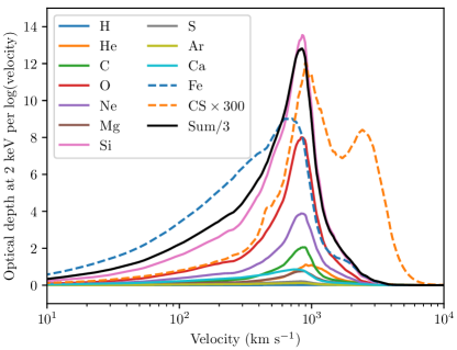
Figure 2: Cumulative direction-averaged optical depth at 10 000 days at 2 keV as a function of velocity for all models (left). The optical depth of the IIb model has been scaled by a factor of 20 for visual clarity. The effect of the cut off at 2400 km s^-1 for the IIb model is expected to be small (Section 3). The density gradient at the inner boundary of the IIb model is very steep because of a much weaker reverse shock, which is a consequence of the lack of a hydrogen envelope. Contribution to the cumulative 2 keV optical depth per $\log(\mathrm{velocity})$ for the B15 model (right). Mathematically, this is $\mathrm{d}\,\tau(\text{2~{}keV})/\mathrm{d}\log(v)$, where $v$ is the velocity. The Compton scattering (CS) contribution and sum have been scaled for visual clarity. The bump at ${\sim}$2500 km s^-1 in the scattering contribution is from hydrogen. The distribution is qualitatively similar for the other models.

The cumulative direction-averaged optical depth at 2 keV as a function of velocity is shown in Figure 2 (left) for all models. The dominant contribution to the optical depth is from ejecta with velocities in the range 400–2000 km s^-1 for the non-stripped models. The velocity range is shifted to higher velocities by a factor of ${\sim}$3 for the IIb model because of the higher average ejecta velocity. We also analyze the contributions to the cumulative distribution from individual elements (Figure 2, right) and find that the general trend is that the contributions from all metals are from approximately the same velocities. There is a trend that contributions from heavier elements are on average from velocities lower than those of lighter elements. The effect of this is less than a factor of a few in velocity, which is comparable to the spread in velocities for individual elements.

4.2 Asymmetries of the Ejecta

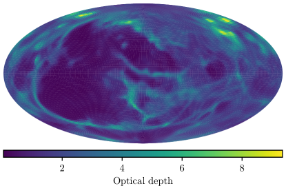
Figure 3: Equal-area Hammer projections of the optical depth at an energy of 2 keV of the B15 (top) and IIb (bottom) models at 10 000 days. The projection looks qualitatively similar at different energies for each of the models. The relative strength of the different structures that can be seen varies across absorption edges because of different compositions.

SN explosions are highly asymmetric and a consequence is that the absorption depends on the line of sight . The projections of the optical depths for all directions of the B15 and IIb models are shown in Figure 3. All models show pronounced asymmetric clumpy structures or filaments. The variances in optical depths are caused by a combination of varying amounts of ejecta expelled in different directions and varying compositions of the ejecta.

We also visually inspected projections of column number densities of individual elements (not shown). The most uniformly distributed elements are the light elements H, He, and C whereas the heavy elements Ca and Fe are most asymmetrically distributed. To a certain extent, the directions of high abundances of heavy elements are anti-correlated with light elements. We interpret this as rising clumps of heavy elements that pierce through the outer shells of the progenitor and leave holes or push the light elements into filaments. It is often the case that the clumps consist of heavier elements whereas the smoother variations and filaments are lighter elements from the outer layers of the progenitor.

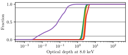
Figure 4: Cumulative distribution functions of the optical depth at 10 000 days as functions of direction. The horizontal gray lines show 90 %, 50 %, and 10 %. The non-stripped models are very similar, while the IIb model has lower optical depths. The iron-peak elements in the IIb model are also more asymmetrically distributed. This is clearly seen from the very wide CDF at 8 keV.

Another representation of asymmetries is the cumulative distribution function (CDF) of the optical depth. In the CDFs, the asymmetries are correlated to the width of the distribution. The optical depth CDFs at 0.5, 8, and 100 keV are shown in Figure 4. The qualitative and quantitative behaviour of the non-stripped models are similar. Optical depths of the IIb model are clearly lower but the distribution of optical depths is also wider. The most notable feature of the CDFs over all directions is the very wide distribution at 8 keV for the IIb model, which is the result of highly asymmetric distribution of iron-peak elements.

Table 4: Asymmetry Measures (1-$\sigma{}$ confidence intervals)

Model	$\tau_{0.5}$	$\tau_{1}$	$\tau_{2}$	$\tau_{4}$	$\tau_{8}$	$\tau_{100}$	$V_{0.5}$	$V_{1}$	$V_{2}$	$V_{4}$	$V_{8}$	$V_{100}$
B15	$171_{-26}^{+30}$	$104_{-17}^{+24}$	$24_{-5}^{+6}$	$4.0_{-0.8}^{+1.0}$	$2.2_{-0.3}^{+0.4}$	$22.6_{-3.5}^{+4.6}\times{}10^{-3}$	$1.4$	$1.5$	$1.6$	$1.6$	$1.4$	$1.4$
N20	$153_{-26}^{+35}$	$175_{-41}^{+70}$	$37_{-9}^{+16}$	$6.0_{-1.3}^{+2.3}$	$2.5_{-0.3}^{+0.4}$	$17.0_{-2.4}^{+3.2}\times{}10^{-3}$	$1.5$	$1.8$	$1.9$	$1.8$	$1.3$	$1.4$
L15	$142_{-26}^{+26}$	$112_{-28}^{+27}$	$22_{-5}^{+5}$	$3.3_{-0.8}^{+0.8}$	$2.1_{-0.4}^{+0.5}$	$18.8_{-0.6}^{+0.7}\times{}10^{-3}$	$1.4$	$1.6$	$1.6$	$1.6$	$1.6$	$1.1$
W15	$221_{-30}^{+34}$	$173_{-36}^{+39}$	$33_{-6}^{+7}$	$4.9_{-0.9}^{+1.0}$	$2.8_{-0.3}^{+1.0}$	$23.6_{-1.4}^{+1.6}\times{}10^{-3}$	$1.3$	$1.6$	$1.5$	$1.5$	$1.5$	$1.1$
IIb	$8_{-3}^{+4}$	$9_{-6}^{+6}$	$2_{-1}^{+1}$	$0.2_{-0.2}^{+0.2}$	$0.1_{-0.1}^{+0.1}$	$\hphantom{0}0.6_{-0.1}^{+0.2}\times{}10^{-3}$	$2.4$	$4.9$	$5.7$	$6.0$	$23.3$	$1.8$

Note. — The 1-$\sigma{}$ confidence intervals of the optical depths refers to the standard deviation of $\tau$ along different directions. This is effectively a measure of the asymmetry of the explosion model.

More quantitative measurements of the asymmetries are given by the variations in optical depths at given energies for each model, which are provided in Table 4. The confidence intervals represent the 1-$\sigma{}$ intervals of the optical depth as a function of direction, which are at a level of approximately 20–40 %. We also include the ratio of the upper bound to the lower bound as a relative measure of asymmetry variance. The optical depth for a given model and energy typically spans a factor of 1.5–2. It is also clear from the variance measures that the IIb model is more asymmetric, in particular around 8 keV where the iron-peak elements dominate the opacity.

4.3 Ejecta Compositions

Figure 5: Probability distribution of the effective slope of the effective cross-section ($\alpha$) for all directions. The effective slope is defined by Equation (2). Different compositions result in different effective cross-sections. Thus, the effective slope serves as a proxy for the composition.

The results up to this point have focused on the direction-averaged optical depth and variance of the optical depth introduced by both asymmetric distribution of material and composition. It is possible to isolate the contribution to the variance of varying composition, which affects the energy-dependence of the optical depth. We do not attempt to quantify the distribution of abundances of all individual elements. Instead, we define the effective slope $\alpha{}$ by

$$\sigma_{\mathrm{SN,eff}}(\boldsymbol{\hat{n}},E)\propto E^{\alpha},$$ (2)

where $\sigma_{\mathrm{SN,eff}}$ is the effective cross-section of the SN ejecta. The general trend is that lighter elements have steeper energy dependencies and heavier elements have shallower dependencies. Therefore, the effective slope can serve as a representation of the variations in compositions as a function of direction. The advantage of introducing $\alpha$ in place of the composition is that the composition depends on eleven parameters (all elements). The drawback is that it provides no insight into the relative abundances of heavier elements, which determine the relative strength of absorption edges. We choose to measure $\alpha$ as the slope between 0.3 and 10 keV.

Figure 5 shows the distribution of $\alpha$ for all directions. The non-stripped models are similar and have distributions that overlap almost completely, whereas the IIb model shows a wider distribution of $\alpha{}$. This is a consequence of the asymmetric distribution of iron-peak elements in the IIb model. For all models, there is a significant spread in the distribution, which indicates that the composition is varying. It is worth pointing out that even though the slope is defined over the range 0.3–10 keV, absorption is often only important in a limited interval where the optical depth is around unity. This is because any lower opacity leaves the spectrum relatively unaffected whereas higher depths are likely to completely obscure the source.

4.4 Compton Scattering

In contrast to photoabsorption, Compton scattering will not destroy the photon, but will result in a down-scattering of the photon energy, until photoabsorption dominates. This was discussed for the early radioactive phase in SN 1987A dominated by ⁵⁶Ni and ⁵⁷Ni decay, as well as for pulsar input (e.g Xu et al., 1988; Ebisuzaki & Shibazaki, 1988; Grebenev & Syunyaev, 1988, and references therein). Here, we limit ourselves to estimates of the optical depths and do not discuss the spectrum resulting from the scattering further.

Figure 1 shows the contribution of Compton scattering to the optical depth. At 10 000 days, the scattering depth above 50 keV is 1–$3\times 10^{-2}$ for the non-stripped models and ${\sim}5\times 10^{-4}$ for the IIb model. The dominating contribution to the scattering depth is by hydrogen and helium. The relative contributions can be seen from the electron column number densities provided in Table 3. Assuming homologous expansion, the scattering depth at 1 MeV is unity at ${\sim}$1000 days for the non-stripped models and ${\sim}$150 days for the IIb model.

The total optical depths above 50 keV are dominated by Compton scattering. The spread in scattering depths can be seen in Figure 4 and Table 4. The RSGs have lower asymmetry variances in the scattering regime. The main reason for this is that scattering is dominated by lighter elements, which are more uniformly distributed in the more extended envelopes of the RSGs.

5 Discussion

5.1 Absorption Properties

The absorption to the central regions of SNRs is high for X-rays for a long time after the explosion. If the ejecta expand homologously, the optical depth below 2 keV remains above unity for more than a century for the non-stripped models and reaches unity at 10 keV at approximately 30 years. The situation is very different for the IIb model. Because the hydrogen envelope is stripped off, the SN explosion expels the ejecta at a factor of 3 higher velocities, which results in a factor of 9 lower optical depths. The contribution of hydrogen to the optical depth constitutes less than ${\sim}10$ % of the total photoabsorption depth above 0.3 keV for all models (Figure 1). The expansion velocity $v$ is also connected to the SN explosion energy $E$ as $v\propto\sqrt{E/M}$, where $M$ is the total ejecta mass. Therefore, it is reasonable to assume that higher explosion energies or lower ejecta masses lead to higher expansion velocities and lower optical depths.

Another important property of ejecta absorption is that the metallicity is much higher than standard ISM abundances. This implies that the hydrogen column density commonly used by X-ray astronomers is a poor parameterization of the absorption. The effective cross-section is much higher for high-metallicity gas than for standard ISM compositions. The energy dependence of the effective cross-section is significantly flatter for metal-rich than metal-poor gas, primarily because high-metallicity gas has more pronounced absorption edges, mostly K-shell edges, in the 0.3–10 keV energy range. The stronger absorption edges are likely to be the most robust observational signature of high-metallicity absorption, because the difference in continuum absorption is likely degenerate with underlying model components.

Compton scattering dominates the optical depth above 50 keV and the energy dependence of the scattering depth is weak for energies lower than 100 keV. The transition energy of 50 keV is higher than for ISM compositions, where the transition occurs at ${\sim}$10 keV. The reason for this is the higher metallicity of the SN ejecta, which significantly increases the importance of photoabsorption and has a much smaller effect on the scattering properties.

5.2 Comparison with Previous Estimates

In general, previous studies find SN ejecta absorption properties comparable to our estimates. However, no previous work has explored 3D SN explosion models, quantified the uncertainties introduced by SN asymmetries, or compared different progenitors.

Fransson & Chevalier (1987) modeled the absorption for X-rays in SN 1987A using the 15-M_☉ 1D model 4A from Woosley et al. (1988). They showed the photoabsorption optical depth in their Figure 1 and found that the optical depth reaches unity at 10 keV at 18 years. This can be compared to our estimates for BSGs, which show that the optical depth at 10 keV reaches unity at ${\sim}$30 years. However, they noted that using the 25-M_☉ model 8A (Woosley et al., 1988) resulted in optical depths that are a factor of 2.2 higher, which better agrees with our results. Fransson & Chevalier (1987) also concluded that Compton scattering starts dominating over photoabsorption in the 30–100 keV range, depending on the composition of the gas.

Serafimovich et al. (2004) used the 15-M_☉ 1D model 14E1 of Blinnikov et al. (2000) to estimate the ejecta absorption in the 1000-year-old pulsar PSR B0540-69.3 in the Large Magellanic Cloud. They reported that the effective cross-section for SN ejecta is 40 times higher than for standard ISM abundances (see Appendix B) and that the effect of ejecta absorption is negligible because of the age of PSR B0540-69.3, which agrees with our results.

Orlando et al. (2015) performed simulations describing SN 1987A and found an ejecta hydrogen column density of ${\sim}3\times 10^{22}$ cm^-2 at 30 years. This number is close to our values of the hydrogen column number densities (Table 3). However, they do not report the chemical composition of the ejecta, which is critical for a complete absorption estimate.

Esposito et al. (2018) used the model lm18a7Ad of Dessart & Hillier (2010, provided to them by S. E. Woosley). It is a 1D model with a total ejecta mass of 15.6 M_☉. Esposito et al. (2018) used the abundances from the model, assumed homogeneous distribution, and estimated the density based on approximations. They reported a hydrogen column density of $7.6\times 10^{21}$ cm^-2 for the ejecta, which should result in absorption properties comparable to our estimates for the abundances provided in their Table 2.

5.3 Sources of Uncertainty

There are several sources of uncertainty that we have neglected. The presented uncertainties on the optical depths in Table 4 only represent the variance introduced by the asymmetries for a given model. One of the purposes of providing column densities for comparable models is to get a handle on the uncertainties associated with the progenitor properties, stellar evolution, and explosion simulations. The sensitivity of the results to progenitor models and early explosion simulations can be estimated by comparing the four non-stripped models. They were not tuned to represent the same progenitor, only B15 and N20 were designed to match the progenitor of SN 1987A in broad terms (see Utrobin et al., 2015). Our results show that the general absorption properties of all non-stripped models are relatively similar. This is most clearly seen from the CDFs in Figure 4 and the values in Table 4. The differences between the direction-averaged properties of the models are comparable to the asymmetry uncertainties within each model. This indicates that the effects of progenitor properties and asymmetry uncertainties are comparable for a given SN type.

Observations of nearby SNRs find dust masses of ${\sim}0.1$ M_☉ or larger in Cas A (Rho et al., 2008; Barlow et al., 2010), the Crab nebula (Gomez et al., 2012; Owen & Barlow, 2015), and SN 1987A (Matsuura et al., 2011, 2015; Indebetouw et al., 2014; Dwek & Arendt, 2015). Molecules composed of metals have also been detected in Cas A (Rho et al., 2012), the Crab nebula (Barlow et al., 2013; Bentley et al., 2018), and SN 1987A (Kamenetzky et al., 2013; Matsuura et al., 2017; Abellán et al., 2017). However, the formation of dust and molecules from the ejecta material only has a small effect on the X-ray absorption properties (Morrison & McCammon, 1983; Draine, 2003). Photoabsorption in soft X-rays is dominated by inner-shell absorption, which is approximately the same for dust and molecules as their constituents and Compton scattering only depends on the electron column density.

Additionally, we do not consider the effects of the compact object kick velocity. A full treatment would require investigation of absorption to all positions that the compact object can have been kicked to, but the 3D kick velocity is rarely known. Some insight into the possible effects of kick velocities on absorption is provided by Figure 2, which shows at what radii the gas contributes to the optical depth. For kick velocities of ${\sim}500$ km s^-1, the maximum effect on the optical depth is ${\sim}50$ % if the kick happens to be aligned with our line-of-sight. For reference, we note that pulsars are inferred from observations to have 3D kick velocities of ${\sim}400\pm{}250$ km s^-1 (Hobbs et al., 2005; Faucher-Giguère & Kaspi, 2006) with some extreme cases up to 1600 km s^-1 (Cordes et al., 1993; Chatterjee & Cordes, 2002, 2004; Hobbs et al., 2005).

5.3.1 Progenitor and Explosion Models

All results rely on the SN progenitors and explosion models. These are not fully self-consistent and it is difficult to exactly quantify the uncertainties introduced by them. We find it unlikely that the model uncertainties have a major, qualitative impact on our conclusions. What follows is a brief description of some of the contributing factors.

The explosion models that we use do not include a longer-lasting phase of simultaneous accretion and mass outflow around the NS after the onset of the explosion as suggested to exist by present self-consistent models (Müller et al., 2017). Having such a phase of accretion and outflow instead of the spherical “wind” that boosts the explosion in the simulations, is likely to lead to more extreme asymmetries in the innermost ${\sim}$0.1 M_☉ of the ejecta. Therefore, the inner half of the iron-group matter is likely to be more asymmetrically distributed. Additionally, the 3D simulations contain no information about mixing below the grid scale, but this is not important for the X-ray absorption properties because the absorption only rely on the total column densities.

Overall, the explosion dynamics is roughly compatible with our present-day knowledge of how neutrino-driven explosions work. Moreover, the asymmetries we find in the simulations are able to produce the mixing needed to explain the light curve of SN 1987A (Utrobin et al., 2015), the morphology of Cas A (Wongwathanarat et al., 2017), or, roughly, the asymmetries of SiO and CO molecules observed in SN 1987A (Abellán et al., 2017). However, an important caveat for the SN 1987A models is that they are based on single-star progenitors. The progenitor of SN 1987A was most likely the result of a merger, which is primarily supported by the triple-ring structure surrounding the SN (Blondin & Lundqvist, 1993; Morris & Podsiadlowski, 2007; Menon & Heger, 2017; Urushibata et al., 2018). The mixing properties of the merger models are different and the mass of the helium and oxygen cores are also much lower than for the single-star progenitors. However, the set of progenitors considered in our study covers a fairly wide range of pre-collapse profiles, and one case (B15) has a core structure with similarities to the core properties of some of the binary models of Menon & Heger (2017).

The relative abundances of the different metals are also uncertain because of the small $\alpha{}$-nuclei networks (see Section 3.1 of Wongwathanarat et al., 2017). This uncertainty only applies to the relative abundances of metals and leaves the total mass and spatial distribution unaffected.

Model B15, despite its ability to yield efficient mixing and to explain the SN 1987A light curve fairly well, is far from being a perfect case for SN 1987A. In particular, the NS mass is too low. A baryonic mass of 1.25 M_☉ corresponds to a gravitational mass of only ${\sim}$1.15 M_☉. It is extremely unlikely that SN 1987A produced a NS with such a record-low mass (cf. Özel & Freire, 2016). This problem is most likely due to the progenitor structure for B15 rather than the explosion modeling.

5.4 Implications for Observations

The high X-ray absorption in young SNRs affects interpretations of observations. We have focused on Cas A and SN 1987A, but the absorption estimates also apply to other extragalactic SNRs. Processes that produce X-rays from young compact objects are thermal surface emission, fallback accretion, and pulsar wind activity. Ejecta absorption obscures any X-ray emission and is generally applicable, but it is possible that extended sources, such as powerful pulsar wind nebulae, produce a significant amount of radiation from outer regions where the absorption is expected to be lower. Another remark on pulsar wind nebulae is that they produce synchrotron emission that extends to high X-ray energies (for a high-energy compilation of the pulsed emission, see Figure 28 of Kuiper & Hermsen, 2015) where Compton scattering is dominating. Given the low scattering depths, the obscuration due to scattering is most likely only important during the first few years.

Another source of high-energy radiation is from radioactive elements synthesized in SN explosions that emit lines in the Compton absorption regime when decaying. This was seen in early observations of SN 1987A (Sunyaev et al., 1987; Dotani et al., 1987; Matz et al., 1988). The first sign of radioactive line emission at intermediate optical depths is the emergence of down-scattered X-ray emission, which is then followed by the direct line emission when the ejecta has expanded further. The time and escaping fluxes of the radioactive emission convey information about the level of mixing of the radioactive elements and could be used to test the accuracy of the SN explosion simulations.

Ejecta absorption can potentially also explain the lack of detection of K-shell emission lines resulting from electron capture in radioactive elements produced by the SN (Leising, 2001, 2006; Theiling & Leising, 2006). Radioactive K-shell lines have been observed in G1.9+0.3, which is the remnant of a thermonuclear SN (Borkowski et al., 2010). Because of the lower mass and higher expansion velocity of Type Ia SNe, the X-ray absorption should be considerably smaller for a given age.

We focus on absorption toward the center of SNRs. The absorption along lines of sight that pierce outer parts of the ejecta have different properties. This is mostly relevant for spatially resolved studies of SNRs. Figure 2 provides some insight into the radial distribution of absorbing gas. We do not attempt to investigate all possible sightlines. The difference introduced by shifting line of sight is not simply a matter of geometrical scaling because the metallicity is higher for paths into the center and lower toward the outer boundary of the ejecta. An effect of this in SN 1987A can be seen in Figures 22 and 23 of Fransson et al. (2013). The penetration of the X-rays from the ring interaction is considerably deeper in the directions of the outer hydrogen envelope compared to the radial penetration in the core direction.

In SN 1987A, the absorption is high and significantly affects observations of the compact object. The analysis is presented in detail in a separate work (Alp et al., 2018). Here we note that the differences in optical depth for the different BSG progenitor models B15 and N20 are less than a factor of 2 and the RSGs also show comparable properties (Section 4). A difference of a factor of 2 in the optical depth approximately corresponds to a factor of two in the allowed luminosities. This uncertainty is comparable to the other uncertainties discussed in Section 5.3.

The effect of absorption is expected to be relatively small for the Galactic SNRs. We find a negligible effect of absorption on the interpretation of Chandra observations of the CCO in Cas A (Appendix A). However, observations of SNRs with higher number of total counts or higher energy resolution should be able to disentangle small effects of ejecta absorption. Our estimates also show that the low-energy X-ray emission from a compact object in a future Galactic SN will be heavily obscured for many decades. It is unlikely that even future telescopes will be able to directly observe emission from newly created compact objects at energies less than ${\sim}5$ keV during the first few decades unless the compact object is very luminous, such as the Crab (Bühler & Blandford, 2014).

6 Summary & Conclusions

Accurate models of absorption are critical for analyses of X-ray observations of SNRs. We use 3D simulations of neutrino-driven SN explosions (Wongwathanarat et al., 2013, 2015) to estimate the column densities of the most abundant elements along the line of sight to the center of the ejecta. The column densities are used to compute the optical depth for X-rays due to photoabsorption and Compton scattering. This provides both the amount and composition of the obscuring gas. We use our absorption models to place new X-ray limits on the compact object in SN 1987A in an accompanying paper (Alp et al., 2018), and re-analyze the X-ray spectrum of the CCO in Cas A (Appendix A). Our main conclusions are the following:

• The optical depth for X-rays is high for a long time after the SN explosion. For the models with a hydrogen envelope, the optical depth between 0.1 and 50 keV is approximately given by $100\,t_{4}^{-2}\,E^{-2}$, where $t_{4}$ is time since the explosion in units of 10 000 days (${\sim}$27 years) and $E$ the energy in units of keV.

• The optical depth above ${\sim}$50 keV is dominated by Compton scattering and is 1–$3\times{}10^{-2}$ at 10 000 days for models with a hydrogen envelope. Scaling backward in time, the scattering depth to the center is unity at around 1000 days after the explosion.

• The optical depth is approximately an order of magnitude lower for the IIb model, which has lost all but 0.5 M_☉ of its hydrogen envelope. This model explodes as a Type IIb SN and shows similarity to Cas A. The optical depth is lower because $\tau\propto 1/(vt)^{2}\propto M/Et^{2}$.

• The expected level of absorption in Cas A based on estimates using the IIb model results in a decrease in the inferred CCO surface temperature of less than ${\sim}1$ % at all epochs, which is lower than the statistical uncertainty. We also find that the ejecta absorption component would be degenerate with the ISM absorption, if ejecta absorption was significant. This is a result of the limited statics of the observation, instrumental energy resolution, and degeneracy with parameters of other model components.

• For the same hydrogen column number density, the metallicity of the SN ejecta is ${\sim}$2 orders of magnitude higher than for the ISM. This implies that the hydrogen column number density is a poor measure of absorption because the effective cross-section is much higher. The high metallicity results in a flatter energy dependence of the cross-section and that the absorption profile has stronger metal edges.

Appendix A Cas A

A.1 Observations and Data Reduction

Table 5: Chandra Cas A CCO Observations

Obs. ID	Start date	Exposure	Source counts	Source fraction
	(YYYY-mm-dd)	(ks)
06690	2006-10-19	61.7	6261	0.958
13783	2012-05-05	63.4	5571	0.953
16946	2015-04-27	68.1	5320	0.954

We analyze the three archival Chandra observations that were performed using an instrumental setup chosen to minimize spectral distortions of the CCO. Details of these observations are presented in Table 5. We reduce the data using CIAO 4.9 and CALDB 4.7.7 (Fruscione et al., 2006) and follow standard data reduction guidelines. No strong background flares are detected and the data are filtered by removing all intervals that deviate from the mean by more than 4$\sigma{}$. All source spectra are extracted from circular regions with radii of 2 pixels (492 mas pixel^-1). All background spectra are extracted from annuli centered on the source position. The inner radii of the annuli are 3 pixels and the outer 5 pixels. The spectra are binned such that the signal-to-noise level is at least 10 in each bin. Spectral fitting is performed using XSPEC version 12.9.1p (Arnaud, 1996).

A.2 Results

Our aim is to investigate if ejecta absorption has a significant effect on the interpretation of the observed spectra of the CCO in Cas A. To do this, we choose a model consisting of thermal emission from a NS surface with a carbon atmosphere, which is modeled using the XSPEC model carbatm (Suleimanov et al., 2014). We use the model tbabs (Wilms et al., 2000) with wilm abundances from Wilms et al. (2000) for the ISM absorption. The ejecta absorption is modeled using the XSPEC model tbvarabs (Wilms et al., 2000), which allows for setting the individual abundances. We take the column densities of the IIb model (Table 3) because it shows similarity to Cas A (Wongwathanarat et al., 2017). All column densities are scaled to 340 years, assuming homologous expansion and ignoring the SNR age difference of the observations. To study an extreme scenario, we scale the average column densities by a factor of 4.1. This value is the ratio of the 99.7^th percentile of the optical depth at 2 keV to the direction-averaged optical depth at 2 keV. This can be interpreted as a 3-$\sigma$ upper limit on the ejecta absorption for the IIb model. The result of scaling to an age of 340 years and taking the 3-$\sigma{}$ upper limit is that the optical depth at 1 keV is ${\sim}$0.2, implying that the total effect of ejecta absorption is expected to be small.

Table 6: Cas A CCO Fitting Results (1-$\sigma{}$ confidence intervals)

Obs.	$N_{\mathrm{ISM}}(\mathrm{H})$	$\tau(1\text{~{}keV})$	$T$	Norm.	$\chi^{2}/\text{d.o.f.}=\chi^{2}_{\mathrm{red}}$
(YYYY)	($10^{22}$ cm-2)		(MK)
No ejecta absorption
2006			$2.07^{+0.05}_{-0.05}$
2012	$2.15^{+0.05}_{-0.05}$	$\cdots$	$2.05^{+0.05}_{-0.05}$	$7.3^{+1.2}_{-1.0}$	$118/134=0.88$
2015			$2.03^{+0.05}_{-0.05}$
3-$\sigma{}$ ejecta absorption
2006			$2.06^{+0.05}_{-0.04}$
2012	$2.01^{+0.05}_{-0.05}$	0.2	$2.04^{+0.05}_{-0.04}$	$7.6^{+1.1}_{-1.1}$	$119/134=0.89$
2015			$2.02^{+0.05}_{-0.04}$
$10\times 3$-$\sigma{}$ ejecta absorption
2006			$1.99^{+0.05}_{-0.05}$
2012	$0.77^{+0.05}_{-0.05}$	2.3	$1.97^{+0.05}_{-0.04}$	$9.7^{+1.6}_{-1.3}$	$123/134=0.92$
2015			$1.95^{+0.04}_{-0.04}$

We perform the fit of the model simultaneously to the three observations. The results of all fits are presented in Table 6. First, we start by ignoring any ejecta absorption. The NS mass is frozen to $1.647$ M_☉ and the radius is frozen to $10.33$ km, to allow for comparisons with previous works (Heinke & Ho, 2010; Posselt et al., 2013). The normalization of the NS carbon atmosphere model is a ratio of the fraction of the surface that is emitting ($A$) over the distance squared in units of 10 kpc. We leave the normalization free to allow for any normalization errors, but tied it across all observations because we do not expect the emitting fraction or distance to change. For a distance of 3.4 kpc, the normalization is 8.65 for $A=1$. The ISM hydrogen column density $N_{\mathrm{ISM}}(\mathrm{H})$ is left free because the absorption toward Cas A is uncertain (Keohane et al., 1996; Salas et al., 2018), but it is tied across observations because it is not expected to vary significantly on these timescales. Additionally, we find no statistically significant improvement by leaving $N_{\mathrm{ISM}}(\mathrm{H})$ untied. The local (unredshifted) blackbody temperature ($T$) is left free.

Next, we include the extreme-case 3-$\sigma{}$ ejecta absorption. The best-fit parameters are shown in the second segment of Table 6. The additional ejecta absorption component has no significant impact and the fit remains essentially unchanged. This is expected because of the low optical depth of ${\sim}$0.2 at 1 keV, which implies that the difference should be very small.

To explore a case of significant absorption, we add another factor of 10 to the 3-$\sigma{}$ absorption. The factor of 10 is arbitrarily chosen but the scenario could represent a case where the IIb model overestimates the bulk expansion velocity or if filamentary structures of higher density have formed along the line of sight. The best-fit values for this case are also provided in Table 6. The fit is statistically slightly worse but still acceptable. The additional ejecta absorption is nearly completely degenerate with the other components, particularly the ISM absorption, but also the temperature and normalization to a certain extent.

The conclusion is that the expected level of ejecta absorption based on our models has an insignificant effect on the estimated temperature of the CCO. The difference in inferred temperature is less than ${\sim}1$ % between the fit without and with 3-$\sigma{}$ ejecta absorption, which is lower than the statistical uncertainty. Additionally, the effect is a similar level of decrease at all epochs, which does not affect investigations of the cooling of the CCO.

Appendix B Comparison with ISM Absorption

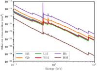
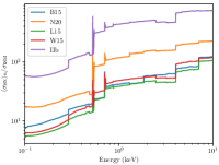
Figure 6: Comparison of the effective cross-sections of the SN ejecta for the five models with the ISM cross-section. The left panel shows the cross-sections as functions of energy and the right panel shows the ratio of the ejecta cross-sections to the ISM cross-section. We note that the SN effective cross-sections are much larger, show shallower energy dependencies, and have much stronger discontinuous absorption features.

A comparison of the SN abundances with the ISM abundances (Wilms et al., 2000) is provided in Table 3. It is common in X-ray astronomy to quantify absorption by the hydrogen column number density and to assume standard abundances of all other elements with respect to hydrogen. This assumption breaks down for ejecta absorption because the metallicity of the SN ejecta is much higher than that of the ISM. The result is that the effective cross-section of the SN ejecta is much higher, falls of slower as a function of energy, and that metal absorption edges are stronger. The effective cross-sections for the five models and the ISM, as well as the ratio of the SN ejecta to ISM cross-sections are shown in Figure 6.

References

- Abellán et al. (2017) Abellán, F. J., Indebetouw, R., Marcaide, J. M., et al. 2017, ApJ, 842, L24, doi: 10.3847/2041-8213/aa784c
- Alp et al. (2018) Alp, D., Larsson, J., Fransson, C., et al. 2018, ArXiv e-prints. https://arxiv.org/abs/1805.04526
- Anders & Grevesse (1989) Anders, E., & Grevesse, N. 1989, Geochim. Cosmochim. Acta, 53, 197, doi: 10.1016/0016-7037(89)90286-X
- Arnaud (1996) Arnaud, K. A. 1996, in Astronomical Society of the Pacific Conference Series, Vol. 101, Astronomical Data Analysis Software and Systems V, ed. G. H. Jacoby & J. Barnes, 17
- Arnett et al. (1989) Arnett, W. D., Bahcall, J. N., Kirshner, R. P., & Woosley, S. E. 1989, ARA&A, 27, 629, doi: 10.1146/annurev.aa.27.090189.003213
- Ashworth (1980) Ashworth, Jr., W. B. 1980, Journal for the History of Astronomy, 11, 1
- Astropy Collaboration et al. (2013) Astropy Collaboration, Robitaille, T. P., Tollerud, E. J., et al. 2013, A&A, 558, A33, doi: 10.1051/0004-6361/201322068
- Barlow et al. (2010) Barlow, M. J., Krause, O., Swinyard, B. M., et al. 2010, A&A, 518, L138, doi: 10.1051/0004-6361/201014585
- Barlow et al. (2013) Barlow, M. J., Swinyard, B. M., Owen, P. J., et al. 2013, Science, 342, 1343, doi: 10.1126/science.1243582
- Bentley et al. (2018) Bentley, R., Wootten, A., Loh, E., et al. 2018, in American Astronomical Society Meeting Abstracts, Vol. 231, American Astronomical Society Meeting Abstracts #231, #241.01
- Bethe & Salpeter (1957) Bethe, H. A., & Salpeter, E. E. 1957, Quantum Mechanics of One- and Two-Electron Atoms (New York: Academic Press, 1957)
- Bionta et al. (1987) Bionta, R. M., Blewitt, G., Bratton, C. B., Casper, D., & Ciocio, A. 1987, Physical Review Letters, 58, 1494, doi: 10.1103/PhysRevLett.58.1494
- Blinnikov et al. (2000) Blinnikov, S., Lundqvist, P., Bartunov, O., Nomoto, K., & Iwamoto, K. 2000, ApJ, 532, 1132, doi: 10.1086/308588
- Blondin & Lundqvist (1993) Blondin, J. M., & Lundqvist, P. 1993, ApJ, 405, 337, doi: 10.1086/172366
- Borkowski et al. (2010) Borkowski, K. J., Reynolds, S. P., Green, D. A., et al. 2010, ApJ, 724, L161, doi: 10.1088/2041-8205/724/2/L161
- Bratton et al. (1988) Bratton, C. B., Casper, D., Ciocio, A., et al. 1988, Phys. Rev. D, 37, 3361, doi: 10.1103/PhysRevD.37.3361
- Bruenn (1993) Bruenn, S. W. 1993, in Nuclear Physics in the Universe, ed. M. W. Guidry & M. R. Strayer, 31–50
- Bühler & Blandford (2014) Bühler, R., & Blandford, R. 2014, Reports on Progress in Physics, 77, 066901, doi: 10.1088/0034-4885/77/6/066901
- Chakrabarty et al. (2001) Chakrabarty, D., Pivovaroff, M. J., Hernquist, L. E., Heyl, J. S., & Narayan, R. 2001, ApJ, 548, 800, doi: 10.1086/318994
- Chatterjee & Cordes (2002) Chatterjee, S., & Cordes, J. M. 2002, ApJ, 575, 407, doi: 10.1086/341139
- Chatterjee & Cordes (2004) —. 2004, ApJ, 600, L51, doi: 10.1086/381498
- Cordes et al. (1993) Cordes, J. M., Romani, R. W., & Lundgren, S. C. 1993, Nature, 362, 133, doi: 10.1038/362133a0
- Davis et al. (2012) Davis, J. E., Bautz, M. W., Dewey, D., et al. 2012, in Proc. SPIE, Vol. 8443, Space Telescopes and Instrumentation 2012: Ultraviolet to Gamma Ray, 84431A
- Dessart & Hillier (2010) Dessart, L., & Hillier, D. J. 2010, MNRAS, 405, 2141, doi: 10.1111/j.1365-2966.2010.16611.x
- Dickey & Lockman (1990) Dickey, J. M., & Lockman, F. J. 1990, ARA&A, 28, 215, doi: 10.1146/annurev.aa.28.090190.001243
- Dotani et al. (1987) Dotani, T., Hayashida, K., Inoue, H., et al. 1987, Nature, 330, 230, doi: 10.1038/330230a0
- Draine (2003) Draine, B. T. 2003, ApJ, 598, 1026, doi: 10.1086/379123
- Dwek & Arendt (2015) Dwek, E., & Arendt, R. G. 2015, ApJ, 810, 75, doi: 10.1088/0004-637X/810/1/75
- Ebisuzaki & Shibazaki (1988) Ebisuzaki, T., & Shibazaki, N. 1988, ApJ, 327, L5, doi: 10.1086/185128
- Elshamouty et al. (2013) Elshamouty, K. G., Heinke, C. O., Sivakoff, G. R., et al. 2013, ApJ, 777, 22, doi: 10.1088/0004-637X/777/1/22
- Esposito et al. (2018) Esposito, P., Rea, N., Lazzati, D., et al. 2018, ApJ, 857, 58, doi: 10.3847/1538-4357/aab6b6
- Faucher-Giguère & Kaspi (2006) Faucher-Giguère, C.-A., & Kaspi, V. M. 2006, ApJ, 643, 332, doi: 10.1086/501516
- Fesen et al. (2006) Fesen, R. A., Hammell, M. C., Morse, J., et al. 2006, ApJ, 645, 283, doi: 10.1086/504254
- Flamsteed (1725) Flamsteed, J. 1725, Historia Coelestis Britannicae, tribus Voluminibus contenta (1675-1689), (1689-1720), vol. 1, 2, 3 (London: H. Meere; in folio; DCC.f.9, DCC.f.10, DCC.f.11)