Vacuum polarization of massive fields in the spacetime of the higher-dimensional black holes.

Abstract

We construct and study the vacuum polarization, $\langle\phi^{2}\rangle_{D},$ of the quantized massive scalar field with a general curvature coupling parameter in higher-dimensional static and spherically-symmetric black hole spacetimes, with a special emphasis put on the electrically charged Tangherlini solutions and the extremal and ultraextremal configurations. For $4\leq D\leq 7$ the explicit analytic expressions for the vacuum polarization are given. For the conformally coupled fields the relation between the trace of the stress-energy tensor and the vacuum polarization is examined, which requires knowledge of the higher-order terms in the Schwinger-DeWitt expansion.

I Introduction

The vacuum polarization, $\langle\phi^{2}\rangle,$ has often been regarded as a lesser cousin to the stress-energy tensor. However, despite the natural interest, there are a few additional reasons to calculate and study $\langle\phi^{2}\rangle.$ Indeed, it plays an important role in symmetry breaking problem and in the calculation of the trace of the stress-energy tensor of the conformally coupled quantum fields, being much easier to find. For example, to construct the stress-energy tensor within the framework of the Schwinger-DeWitt approach, one has to functionally differentiate the effective action with respect to the metric tensor whereas to calculate the vacuum polarization it is sufficient to use the Green function. Moreover, the calculations of the vacuum polarization may reveal conceptual subtleties of the problem and help to choose the best calculational strategy. Generally speaking, if there are some technical problems in the calculations of $\langle\phi^{2}\rangle$ the same is expected in construction of the stress-energy tensor. On the other hand, if the calculation of the vacuum polarization goes smoothly the same is expected for the stress-energy-tensor. In the latter case the only difference is the scale of the calculations.

Starting with the seminal work of Candelas Candelas (1980), the vacuum polarization has been, and currently is, studied in a number of physically interesting cases, as for example, Schwarzschild black holes or FRWL cosmologies  Candelas (1980); Candelas and Howard (1984); Anderson (1990); Frolov (1982); Anderson (1989); Fawcett and Whiting (1981); Fawcett (1983); Kofman and Sahni (1983); Anderson et al. (1995); Shiraishi (1992); Quinta et al. (2016); Popov (2004); Flachi and Tanaka (2008); Tomimatsu and Koyama (2000); Koyama et al. (2000); Matyjasek et al. (2010); Popov (2016); Levi and Ori (2016). The vacuum polarization effects have been analyzed in the spacetimes of distorted black holes Frolov and Garcia (1983); Frolov and Sanchez (1986), in the spacetimes of dimension higher (or smaller) than 4 Frolov et al. (1989); Shiraishi and Maki (1994a, b); Thompson and Lemos (2009); Matyjasek and Sadurski (2015, 2014); Quinta et al. (2018); Taylor and Breen (2017, 2016); Flachi et al. (2016); Breen et al. (2015). Approximate expressions describing $\langle\phi^{2}\rangle$ have been constructed in Refs. Page (1982); Frolov and Zelnikov (1987, 1984); Frolov (1986); Matyjasek (1996).

The aim of this paper is to construct the vacuum polarization of a quantized massive scalar field (with arbitrary curvature coupling) satisfying the covariant equation

$$\left(-\Box+m^{2}+\xi R\right)\phi=0,$$ (1)

where $m$ is the mass of the field, $\xi$ is the coupling constant and $R$ is the Ricci scalar, in a general $D$-dimensional static and spherically-symmetric spacetime described by the line element

$$ds^{2}=-f(r)dt^{2}+h(r)dr^{2}+r^{2}d\Omega^{2}_{D-2},$$ (2)

where $d\Omega^{2}_{D-2}$ is the metric on a unit $(D-2)$-dimensional sphere, and to apply the general formulas in the spacetime of the charged black hole. The line element describing such configurations has been constructed by Tangherlini in the early sixties. It has a particularly simple and transparent form when parametrized by the radial coordinates of the event and inner horizons, denoted respectively by $r_{+}$ and $r_{-}.$ The charged Tangherlini solution has the form (2) with

$$f(r)=\frac{1}{h(r)}=\left[1-\left(\frac{r_{+}}{r}\right)^{D-3}\right]\left[1-\left(\frac{r_{-}}{r}\right)^{D-3}\right].$$ (3)

Making use of the relations

$$M=\frac{D-2}{16\pi}\Omega_{D-2}\left(r_{+}^{D-2}+r_{-}^{D-2}\right)$$ (4)

and

$$Q=\pm\left(r_{+}r_{-}\right)^{\frac{D-3}{2}}\sqrt{\frac{(D-3)(D-2)}{8\pi}},$$ (5)

where $\Omega_{D-2}$ is the area of a unit $(D-2)$-sphere, the line element can be expressed in a standard mass, charge parametrization. The area of the $(D-2)$-dimensional sphere is given by

$$\Omega_{D-2}=\frac{2\pi^{\frac{D-1}{2}}}{\Gamma(\frac{D-1}{2})}.$$ (6)

When the horizons merge, i. e., $(r_{+}=r_{-}=r_{\pm})$ the topology of the closest vicinity of the horizon of the extremal black hole is $AdS_{2}\times S^{D-2},$ and the geometry, when expanded into the whole manifold, is a special case of the general solution

$$ds^{2}=\frac{1}{A}\left(-\sinh^{2}\chi d\tau^{2}+d\chi^{2}\right)+Bd\Omega^{2}_{D-2},$$ (7)

where $A,B\in\mathbb{R}.$ It is a product spacetime with maximally symmetric subspaces. Sometimes it is advantageous to work with the

$$ds^{2}=\frac{1}{Ay^{2}}\left(-dT^{2}+dy^{2}\right)+Bd\Omega^{2}_{D-2}.$$ (8)

The equation (7) describes the vicinity of the extremal black hole (2) provided $A=f^{\prime\prime}(r_{\pm})/2$ and $B=r_{\pm}^{2}.$ Consequently,

$$A=\frac{(D-3)^{2}}{r_{\pm}^{2}}$$ (9)

and in $D=4$ one has the Bertotti-Robinson solution.

The calculations of the stress-energy tensor and the vacuum polarization of the quantized fields in curved spacetimes are extremely hard as they exhibit a nonlocal dependence on the spacetime metric. Here we consider the case when the Compton length associated with the field, $\lambda_{c},$ satisfies the condition

$$\frac{\lambda_{c}}{L}\ll 1,$$ (10)

where $L$ is a characteristic radius of the curvature of the background geometry, and, consequently, the nonlocal contribution to the vacuum polarization can be neglected Frolov and Zelnikov (1984); Matyjasek (2000, 2001); Matyjasek and Sadurski (2015).

In the proper-time formalism one assumes that the Green function, $G(x,x^{\prime}),$ that satisfies the equation

$$\left(\Box-m^{2}-\xi R\right)G(x,x^{\prime})=-\delta(x,x^{\prime}),$$ (11)

is given by

$$G^{F}(x,x^{\prime})=\frac{i\Delta^{1/2}}{(4\pi)^{D/2}}\int_{0}^{\infty}ids\frac{1}{(is)^{D/2}}\exp\left[-im^{2}s+\frac{i\sigma(x,x^{\prime})}{2s}\right]A(x,x^{\prime};is),$$ (12)

where

$$A(x,x^{\prime};is)=\sum_{k=0}^{\infty}(is)^{k}a_{k}(x,x^{\prime}),$$ (13)

$s$ is the proper time and the biscalars $a_{k}(x,x^{\prime})$ are the celebrated Hadamard-DeWitt coefficients, $\Delta(x,x^{\prime})$ is the vanVleck-Morette determinant and the biscalar $\sigma(x,x^{\prime})$ is defined as the one-half of the geodetic distance between $x$ and $x^{\prime}.$ Now, let us define

$$A^{(n)}_{reg}(x,x^{\prime};is)=A(x,x^{\prime};is)-\sum_{k=0}^{[\frac{D}{2}]-1}a_{k}(x,x^{\prime})(is)^{k},$$ (14)

where $\lfloor x\rfloor$ (a floor function) gives the largest integer less than or equal $x,$ substitute in Eq. (12) $A^{(D)}_{reg}(x,x^{\prime};is)$ for $A(x,x^{\prime};is)$ and finally denote the thus obtained biscalar by $G^{(D)}_{reg}.$ The field fluctuation that characterizes the vacuum polarization in the $D$-dimensional spacetime is defined as

$$\langle\phi^{2}\rangle=-i\lim_{x^{\prime}\to x}G^{(D)}_{reg}.$$ (15)

Making the substitution $m^{2}\to m^{2}-i\varepsilon$ ($\varepsilon>0$) the integral (12) can easily be calculated Matyjasek and Sadurski (2014, 2015):

$$\langle\phi^{2}\rangle=\frac{1}{(4\pi)^{D/2}}\sum_{k=\lfloor D/2\rfloor}^{N}\frac{a_{k}}{(m^{2})^{k+1-D/2}}\Gamma\big{(}k+1-\frac{D}{2}\big{)},$$ (16)

where the coincidence limit of the Hadamard-DeWitt biscalars is defined as $a_{k}=\lim_{x^{\prime}\to x}a_{k}(x,x^{\prime})$ and the upper sum limit, $N,$ remains us that only a first few Hadamard-DeWitt coefficients are known. One expects that if the condition (10) holds Eq. (16) gives a reasonable approximation to the exact $\langle\phi^{2}\rangle.$ Eq. (16) is generalization to arbitrary dimension of the formula derived by Frolov Frolov (1986) and coincides with the result obtained in Ref. Thompson and Lemos (2009).

The plan of the paper is as follows. In the next section (subsections II.1 and II.2) we shall construct the vacuum polarization of the quantized massive field in the general static and spherically-symmetric $D$-dimensional spacetime $(4\leq D\leq 7)$ and use the obtained formulas in the spacetime of the charged Tangherlini black holes. The special emphasis is put on the extremal and ultraextremal configurations. In the section II.3 we shall analyze the trace of the stress-energy tensor of the conformally coupled massive fields and analyze its relation to the vacuum polarization. The last section III concludes the paper with some final remarks, putting our results in a somewhat broader perspective. Our general results for $\langle\phi^{2}\rangle$ in $D$-dimensional black hole spacetime are relegated to Appendix.

Throughout the paper the natural system of unit is used. The signature of the metric is “ mainly positive” $(-,+,...,+)$ and our conventions for curvature are $R^{a}_{\ bcd}=\partial_{c}\Gamma^{a}_{bd}...$ and $R^{a}_{\ bac}=R_{bc}.$

II $\langle\phi^{2}\rangle$ in the spacetime of $D$-dimensional static and spherically-symmetric black hole.

The formula (16) shows that the Hadamard-DeWitt coefficients can be used in a twofold way: Firstly, for a given dimension the lowest coefficient of the expansion gives the leading approximation to the vacuum polarization, whereas the higher order coefficients give the higher-order terms in (16). On the other hand, we can confine ourselves only to the main approximation and use the coefficients in various dimensions. Moreover, for the conformally coupled fields with $\xi=(D-2)/(4D-4)$ one has a very interesting formula that relates the trace of the quantized stress-energy tensor and the vacuum polarization.

In this paper we shall restrict our analyses to $4\leq D\leq 7$ and use the first three nontrivial coefficients ($a_{2},$ $a_{3},$ and $a_{4}$) to calculate all the terms from Table 1. Since the results for the higher-order terms as well as these for $D>7$ are rather complicated, to prevent unnecessary proliferation of lengthy and not very illuminating formulas, they will be not presented here. (The only exception is Sec. II.3).

As can be seen in Table 1 the possible applications of the Hadamard-DeWitt coefficients are of course wider.

$D$	1st	2nd	3rd
4	$a_{2}$	$a_{3}$	$a_{4}$
5	$a_{2}$	$a_{3}$	$a_{4}$
6	$a_{3}$	$a_{4}$
7	$a_{3}$	$a_{4}$
8	$a_{4}$
9	$a_{4}$

Table 1: The rows (from left to right) represent the dimension of the spacetime, the leading terms, the next-to-leading and the next-to-next-to-leading terms of the expansion (16).

Indeed, the coefficients $a_{i}$ for $(i\geq 3)$ play a crucial role in calculations of the stress-energy tensor of the quantized massive fields in a large mass limit, giving the unique possibility to study the dependence of the quantum effects on the dimension of the background spacetime. In this case the entries in Tab. 1 should be moved one column to the left, as the main approximation of the stress-energy tensor in $D=4$ and 5 requires $a_{3},$ whereas $a_{4}$ is needed in the calculation of the main approximation in $D=6$ and 7.

If there are $N$ scalar fields $\phi_{i},$ each with a different mass $m_{i},$ then all formulas remain intact provided the following change is made

$$\frac{1}{m^{2}}=\sum_{i=1}^{N}\frac{1}{m_{i}^{2}}.$$ (17)

This also shows that the quantum effects can be made great by taking large number of the quantized fields.

II.1 D = 4 and D = 5

Inspection of the general formula (16) shows that to calculate the vacuum polarization of the massive scalar field one needs the coincidence limit of the Hadamard-DeWitt coefficient $a_{2},$ which is constructed from the curvature invariants $R_{abcd}R^{abcd},$ $R_{ab}R^{ab},$ $R^{2}$ and $\Box R.$ Although it looks quite simple, the resulting expression for $\langle\phi^{2}\rangle$ constructed for a general metric (2) is complicated. Indeed, taking $a_{2}$ in the form

$$a_{2}=\frac{1}{180}R_{abcd}R^{abcd}-\frac{1}{180}R_{ab}R^{ab}+\frac{1}{6}\left(\frac{1}{5}-\xi\right)R_{;a}^{\phantom{a}a}+\frac{1}{2}\left(\frac{1}{6}-\xi\right)^{2}R^{2},$$ (18)

after some algebra, one has

$$\langle\phi^{2}\rangle_{D}=\frac{1}{K}\sum_{l=0}^{2}\sum_{k=1}^{13}\alpha_{k}^{i}\xi^{i}F_{k}(r),$$ (19)

where

$$K=\begin{cases}16\pi^{2}m^{2}&\text{if $D=4$}\\ 32\pi^{2}m&\text{if $D=5$}\end{cases}$$ (20)

and the functions $F_{k}$ (the same for both dimensions) as well as the dimension-dependent coefficients $\alpha_{k}^{i}$ are shown in Table 2.

Since the general form of the vacuum polarization can easily be inferred form Table 2 it will not be presented explicitly here. Instead, we shall discuss its behavior in a few important regimes. First, let us consider the simplest case of the four-dimensional black holes. On general grounds one expects that for the line element (3) the result falls as $r^{-6}$ and the most interesting region is the vicinity of the event horizon. For the physical values of the coupling constant, i.e., for $\xi=0$ and $\xi=1/6,$ the general expression calculated at the event horizon reduces to

$$K\langle\phi^{2}\rangle_{4}=-\frac{f^{\prime\prime}}{18r_{+}^{2}}+\frac{1}{60}{f^{\prime\prime}}^{2}-\frac{f^{\prime}}{3r_{+}^{3}}+\frac{13{f^{\prime}}^{2}}{45r_{+}^{2}}-\frac{1}{30}f^{(3)}f^{\prime}-\frac{f^{\prime}f^{\prime\prime}}{30r_{+}}+\frac{1}{15r_{+}^{4}}$$ (21)

and

$$K\langle\phi^{2}\rangle_{4}=\frac{1}{360}{f^{\prime\prime}}^{2}+\frac{{f^{\prime}}^{2}}{90r_{+}^{2}}-\frac{1}{180}f^{(3)}f^{\prime}-\frac{f^{\prime}f^{\prime\prime}}{30r_{+}}+\frac{1}{90r_{+}^{4}},$$ (22)

respectively.

Now, let us assume that the black hole is extremal, i.e., the event and the inner horizons coincide and analyze the vacuum polarization on the degenerate horizon. It means that $f(r_{\pm})=f^{\prime}(r_{\pm})=0$ and from the previous analysis we know that the same result can be obtained calculating the vacuum polarization in the product spacetime with the maximally symmetric subspaces. Inspection of Table 2 gives the following expression for the vacuum polarization in the spacetime of the extreme black hole

$$K\langle\phi^{2}\rangle_{4}=-\frac{f^{\prime\prime}}{18r_{\pm}^{2}}+\xi^{2}\left(-\frac{2f^{\prime\prime}}{r_{\pm}^{2}}+\frac{1}{2}f^{\prime\prime 2}+\frac{2}{r_{\pm}}^{4}\right)+\xi\left(\frac{2f^{\prime\prime}}{3r_{\pm}^{2}}-\frac{1}{6}f^{\prime\prime 2}-\frac{2}{3r_{\pm}^{4}}\right)+\frac{1}{60}f^{\prime\prime 2}+\frac{1}{15r_{\pm}^{4}}.$$ (23)

If additionally the second derivative of the function $f$ at the event horizon vanishes one has the Plebanski-Hacyan geometry with

$$K\langle\phi^{2}\rangle_{4}=\frac{2\xi^{2}}{r_{+}^{4}}-\frac{2\xi}{3r_{+}^{4}}+\frac{1}{15r_{+}^{4}}.$$ (24)

Similarly, at the event horizon of the five-dimensional black hole one has for the minimal coupling

$$K\langle\phi^{2}\rangle_{5}=-\frac{f^{\prime\prime}}{6r_{+}^{2}}+\frac{1}{60}{f^{\prime\prime}}^{2}-\frac{4f^{\prime}}{3r_{+}^{3}}+\frac{59{f^{\prime}}^{2}}{120r_{+}^{2}}-\frac{1}{30}f^{(3)}f^{\prime}-\frac{f^{\prime}f^{\prime\prime}}{20r_{+}}+\frac{1}{2r_{+}^{4}}$$ (25)

and for the conformal coupling

$$K\langle\phi^{2}\rangle_{5}=\frac{1}{64}\left(-\frac{f^{\prime\prime}(r)}{6r_{+}^{2}}+\frac{23}{120}f^{\prime\prime 2}+\frac{5f^{\prime}}{3r_{+}^{3}}-\frac{f^{\prime 2}}{30r_{+}^{2}}-\frac{2}{15}f^{(3)}f^{\prime}-\frac{17f^{\prime}f^{\prime\prime}}{10r_{+}}+\frac{1}{2r_{+}^{4}}\right).$$ (26)

The vacuum polarization of the extremal black hole is given by

$$K\langle\phi^{2}\rangle_{5}=-\frac{f^{\prime\prime}}{6r_{\pm}^{2}}+\xi^{2}\left(-\frac{6f^{\prime\prime}}{r_{\pm}^{2}}+\frac{1}{2}{f^{\prime\prime}}^{2}+\frac{18}{r_{\pm}^{4}}\right)+\xi\left(\frac{2f^{\prime\prime}}{r_{\pm}^{2}}-\frac{1}{6}{f^{\prime\prime}}^{2}-\frac{6}{r_{\pm}^{4}}\right)+\frac{1}{60}{f^{\prime\prime}}^{2}+\frac{1}{2r_{\pm}^{4}}$$ (27)

whereas for the ultraextremal configuration, one has

$$K\langle\phi^{2}\rangle_{5}=\frac{18\xi^{2}}{r_{\pm}^{4}}-\frac{6\xi}{r_{\pm}^{4}}+\frac{1}{2r_{\pm}^{4}}.$$ (28)

Finally, let us return to the charged black holes and introduce new variables, $x$ and $\beta,$ defined as $x=r/r_{+}$ and $\beta=r_{-}/r_{+}.$ Simple calculation give

$$K\langle\phi^{2}\rangle_{4}=\frac{1}{15r_{+}^{4}}\left[\frac{1}{x^{6}}\left(1+2\beta+\beta^{2}\right)-\frac{4}{x^{7}}\left(\beta+\beta^{2}\right)+\frac{13}{3x^{8}}\beta^{2}\right]$$ (29)

and

$$K\langle\phi^{2}\rangle_{5} = \frac{1}{5r_{+}^{4}}\left[\frac{1}{x^{8}}\left(2\beta^{4}-4\beta^{2}+40\beta^{2}\xi+2\right)\right.$$ (30)

$$\left.+\frac{1}{x^{10}}\left(2\beta^{4}+2\beta^{2}-60\beta^{4}\xi-60\beta^{2}\xi\right)+\frac{1}{x^{12}}\left(-\frac{17\beta^{4}}{6}+10\beta^{4}\xi^{2}+\frac{230\beta^{4}\xi}{3}\right)\right].$$

The higher order terms constructed from $a_{3}$ and $a_{4}$ can be found in Ref. Matyjasek et al. (2010) and the results presented in this section generalize those of Lemos and Thompson Thompson and Lemos (2009).

Inspection of Eq. (29) shows that that the result (that is independent of $\xi$) is always positive on the event horizon and is tends to $0^{+}$ as $x\to\infty,$ whereas in $(D=5)$-case the vacuum polarization exhibits the more complicated dependence on the coupling parameter. The asymptotic behavior of the latter is shown in Fig. I. The vacuum polarization at the event horizon is always nonnegative for the minimal and the conformal coupling.

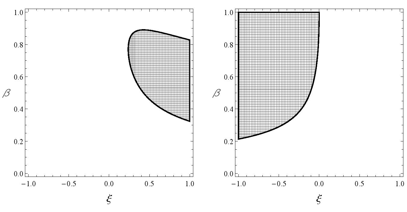
Figure 1: The shaded regions in the $(\xi,\beta)$-space, in which the field fluctuation is negative at the event horizon (left panel). The shaded region in the right panel represents points with the property $\langle\phi^{2}\rangle_{5}\to 0^{-}$ as $r\to\infty.$

Since the second derivative of $f$ calculated at the event horizon is $f^{\prime\prime}=2/r_{\pm}^{2}$ and $f^{\prime\prime}=8/r_{\pm}^{2}$ one has

$$K\langle\phi^{2}\rangle_{4}=\frac{1}{45r_{\pm}^{2}}$$ (31)

and

$$K\langle\phi^{2}\rangle_{5}=\frac{1}{r_{\pm}^{4}}\left(\frac{7}{30}-\frac{2}{3}\xi+2\xi^{2}\right),$$ (32)

respectively.

II.2 D = 6 and D = 7

In this section we shall analyze the approximation to the field fluctuation of the quantized massive fields in $D=6$ and $D=7.$ The coincidence limit of the Hadamard-DeWitt biscalar $a_{3}(x,x^{\prime})$ is much more complicated than the coefficient $a_{2}$ and can be written in the form that is valid in any dimension

$$a_{3}=\frac{1}{7!}b_{3}^{(0)}+\frac{1}{360}b_{3}^{(\xi)},$$ (33)

where

$$b_{3}^{(0)} = \frac{35}{9}R^{3}+17R_{;a}^{\phantom{;\phantom{a}}}R_{\phantom{;\phantom{a}}}^{;a}-2R_{ab;c}^{\phantom{a}\phantom{b}\phantom{;\phantom{c}}}R_{\phantom{a}\phantom{b}\phantom{;\phantom{c}}}^{ab;c}-4R_{ab;c}^{\phantom{a}\phantom{b}\phantom{;\phantom{c}}}R_{\phantom{a}\phantom{c}\phantom{;\phantom{b}}}^{ac;b}+9R_{abcd;e}^{\phantom{a}\phantom{b}\phantom{c}\phantom{d}\phantom{;\phantom{e}}}R_{\phantom{a}\phantom{b}\phantom{c}\phantom{d}\phantom{;\phantom{e}}}^{abcd;e}+28RR_{;a\phantom{a}}^{\phantom{;\phantom{a}}a}+18R_{;a\phantom{a}b\phantom{b}}^{\phantom{;\phantom{a}}a\phantom{b}b}$$ (34)

$$-8R_{ab;c\phantom{c}}^{\phantom{a}\phantom{b}\phantom{;\phantom{c}}c}R_{\phantom{a}\phantom{b}}^{ab}-\frac{14}{3}RR_{ab}^{\phantom{a}\phantom{b}}R_{\phantom{a}\phantom{b}}^{ab}+24R_{ab;c\phantom{b}}^{\phantom{a}\phantom{b}\phantom{;\phantom{c}}b}R_{\phantom{a}\phantom{c}}^{ac}-\frac{208}{9}R_{ab}^{\phantom{a}\phantom{b}}R_{c\phantom{a}}^{\phantom{c}a}R_{\phantom{b}\phantom{c}}^{bc}+12R_{\phantom{a}\phantom{b}\phantom{c}\phantom{d};e\phantom{e}}^{abcd\phantom{;\phantom{e}}e}R_{abcd}^{\phantom{a}\phantom{b}\phantom{c}\phantom{d}}$$

$$+\frac{64}{3}R_{ab}^{\phantom{a}\phantom{b}}R_{cd}^{\phantom{c}\phantom{d}}R_{\phantom{a}\phantom{c}\phantom{b}\phantom{d}}^{acbd}+\frac{16}{3}R_{ab}^{\phantom{a}\phantom{b}}R_{cde\phantom{a}}^{\phantom{c}\phantom{d}\phantom{e}a}R_{\phantom{b}\phantom{e}\phantom{c}\phantom{d}}^{becd}+\frac{80}{9}R_{abcd}^{\phantom{a}\phantom{b}\phantom{c}\phantom{d}}R_{e\phantom{a}f\phantom{c}}^{\phantom{e}a\phantom{f}c}R_{\phantom{b}\phantom{e}\phantom{d}\phantom{f}}^{bedf}+\frac{44}{9}R_{abcd}^{\phantom{a}\phantom{b}\phantom{c}\phantom{d}}R_{ef\phantom{a}\phantom{b}}^{\phantom{e}\phantom{f}ab}R_{\phantom{c}\phantom{d}\phantom{e}\phantom{f}}^{cdef}$$

$$+\frac{14}{3}RR_{abcd}^{\phantom{a}\phantom{b}\phantom{c}\phantom{d}}R_{\phantom{a}\phantom{b}\phantom{c}\phantom{d}}^{abcd}$$

and

$$b_{3}^{(\xi)} = -5R^{3}\xi+30R^{3}\xi^{2}-60R^{3}\xi^{3}-12\xi R_{;a}^{\phantom{;\phantom{a}}}R_{\phantom{;\phantom{a}}}^{;a}+30\xi^{2}R_{;a}^{\phantom{;\phantom{a}}}R_{\phantom{;\phantom{a}}}^{;a}-22R\xi R_{;a\phantom{a}}^{\phantom{;\phantom{a}}a}+60R\xi^{2}R_{;a\phantom{a}}^{\phantom{;\phantom{a}}a}$$ (35)

$$-6\xi R_{;a\phantom{a}b\phantom{b}}^{\phantom{;\phantom{a}}a\phantom{b}b}-4\xi R_{;ab}^{\phantom{;\phantom{a}}\phantom{b}}R_{\phantom{a}\phantom{b}}^{ab}+2R\xi R_{ab}^{\phantom{a}\phantom{b}}R_{\phantom{a}\phantom{b}}^{ab}-2R\xi R_{abcd}^{\phantom{a}\phantom{b}\phantom{c}\phantom{d}}R_{\phantom{a}\phantom{b}\phantom{c}\phantom{d}}^{abcd}.$$

A closer inspection of the coefficient $a_{3}$ shows that it is a sum of the curvature invariants constructed from the Riemann tensor, its covariant derivatives and contractions. In general, the coefficient $[a_{n}]$ (for a given spin) is a linear combination of the Riemann invariants and belongs to $\bigoplus_{q=1}^{n}{\cal R}_{2n,q}^{0},$ where ${\cal R}_{s,q}^{r}$ is a vector space of Riemannian polynomials of rank $r$ (the number of free tensor indices), order $s$ (number of derivatives) and degree $q$ (number of factors). The type of the field is encoded in the coefficients of the linear combination.

Now the vacuum fluctuation has a general form

$$\langle\phi^{2}\rangle_{D}=\frac{1}{K}\sum_{l=0}^{3}\sum_{k=1}^{36}\alpha_{k}^{i}\xi^{i}F_{k}(r),$$ (36)

where

$$K=\begin{cases}64\pi^{3}m^{2}&\text{if $D=6$}\\ 128\pi^{3}m&\text{if $D=7$}\end{cases}$$ (37)

and the functions $F_{k}$ and the (dimension-dependent) coefficients $\alpha_{k}$ are listed in Tables III-V. Once again we shall not present the general result for $\langle\phi^{2}\rangle_{D}$ as it can easily be obtained form the tables. Instead we shall confine ourselves to the physically important limits.

Following the steps form the previous section, for the vacuum polarization at the event horizon of the minimally coupled field one has

$$K\langle\phi^{2}\rangle_{6} = -\frac{29f^{\prime\prime}}{90r_{+}^{4}}+\frac{{f^{\prime\prime}}^{2}}{30r_{+}^{2}}-\frac{1}{630}{f^{\prime\prime}}^{3}-\frac{58f^{\prime}}{15r_{+}^{5}}+\frac{116f^{\prime 2}}{45r_{+}^{4}}-\frac{2f^{\prime 3}}{315r_{+}^{3}}-\frac{1}{140}f^{(4)}f^{\prime 2}$$ (38)

$$-\frac{f^{(3)}f^{\prime}}{15r_{+}^{2}}-\frac{8f^{(3)}f^{\prime 2}}{315r_{+}}-\frac{f^{\prime}f^{\prime\prime}}{15r_{+}^{3}}+\frac{131f^{\prime 2}f^{\prime\prime}}{630r_{+}^{2}}+\frac{2f^{\prime}{f^{\prime\prime}}^{2}}{315r_{+}}+\frac{1}{210}f^{(3)}f^{\prime}f^{\prime\prime}+\frac{74}{63r_{+}^{6}},$$

whereas the analogous result for the conformally coupled fields is given by

$$K\langle\phi^{2}\rangle_{6} = \frac{f^{\prime\prime}}{2250r_{+}^{4}}-\frac{{f^{\prime\prime}}^{2}}{750r_{+}^{2}}-\frac{2{f^{\prime\prime}}^{3}}{7875}-\frac{2f^{\prime}}{375r_{+}^{5}}-\frac{16{f^{\prime}}^{2}}{1125r_{+}^{4}}+\frac{2{f^{\prime}}^{3}}{2625r_{+}^{3}}-\frac{f^{(4)}{f^{\prime}}^{2}}{2100}$$ (39)

$$-\frac{4f^{(3)}{f^{\prime}}^{2}}{525r_{+}}+\frac{7f^{\prime}f^{\prime\prime}}{375r_{+}^{3}}-\frac{113{f^{\prime}}^{2}f^{\prime\prime}}{15750r_{+}^{2}}-\frac{13f^{\prime}{f^{\prime\prime}}^{2}}{7875r_{+}}+\frac{1}{700}f^{(3)}f^{\prime}f^{\prime\prime}-\frac{74}{7875r_{+}^{6}}.$$

Usually, the quantum effects of the massive fields are most pronounced at the event horizon and its closest vicinity. For the extremal and ultraetremal configurations one has

$$K\langle\phi^{2}\rangle_{6} = -\frac{29f^{\prime\prime}}{90r_{\pm}^{4}}+\frac{f^{\prime\prime 2}}{30r_{\pm}^{2}}-\frac{1}{630}f^{\prime\prime 3}+\frac{74}{63r_{\pm}^{6}}+\xi^{3}\left(\frac{72f^{\prime\prime}}{r_{\pm}^{4}}-\frac{6f^{\prime\prime 2}}{r_{\pm}^{2}}+\frac{1}{6}f^{\prime\prime 3}-\frac{288}{r_{\pm}^{6}}\right)$$ (40)

$$+\xi^{2}\left(-\frac{36f^{\prime\prime}}{r_{\pm}^{4}}+\frac{3f^{\prime\prime 2}}{r_{\pm}^{2}}-\frac{1}{12}f^{\prime\prime 3}+\frac{144}{r_{\pm}^{6}}\right)+\xi\left(\frac{89f^{\prime\prime}}{15r_{\pm}^{4}}-\frac{8f^{\prime\prime 2}}{15r_{\pm}^{2}}+\frac{1}{60}f^{\prime\prime 3}-\frac{116}{5r_{\pm}^{6}}\right)$$

and

$$K\langle\phi^{2}\rangle_{6}=-\frac{288\xi^{3}}{r_{\pm}^{6}}+\frac{144\xi^{2}}{r_{\pm}^{6}}-\frac{116\xi}{5r_{\pm}^{6}}+\frac{74}{63r_{\pm}^{6}},$$ (41)

respectively.

Thus far our results have been valid for any static and spherically-symmetric metric. Now let us consider the charged Tangherlini solution. Simple manipulations give

$$\langle\phi^{2}\rangle_{6} = \frac{1}{r_{+}^{6}}\left[\frac{1}{x^{12}}\left(15\beta^{6}-30\beta^{3}+280\beta^{3}\xi+15\right)+\frac{\eta}{x^{15}}\left(-\frac{1333\beta^{6}}{63}+\frac{3382\beta^{3}}{63}-1232\beta^{3}\xi-\frac{1333}{63}\right)\right.$$ (42)

$$+\frac{\beta^{3}}{x^{18}}\left(\frac{907\beta^{6}}{105}-\frac{1250\beta^{3}}{21}+432\beta^{3}\xi^{2}+\frac{5448\beta^{6}\xi}{5}+\frac{21576\beta^{3}\xi}{5}+\frac{5448\xi}{5}+\frac{907}{105}\right)$$

$$\left.+\frac{\beta^{6}\eta}{x^{21}}\left(-576\xi^{2}-\frac{16736\xi}{5}-\frac{88}{35}\right)+\frac{\beta^{9}}{x^{24}}\left(36\xi^{3}+702\xi^{2}+2392\xi+\frac{6761}{315}\right)\right],$$

where $\eta=1+\beta^{3}.$ The sign of the vacuum polarization at the event horizon as well as its asymptotic behavior as $r\to\infty$ is shown in Fig. 2. Specifically, the vacuum polarization at the event horizon is always negative for the minimal coupling. On the other hand, for the conformal coupling, it is positive for $0.683<\xi<0.762.$

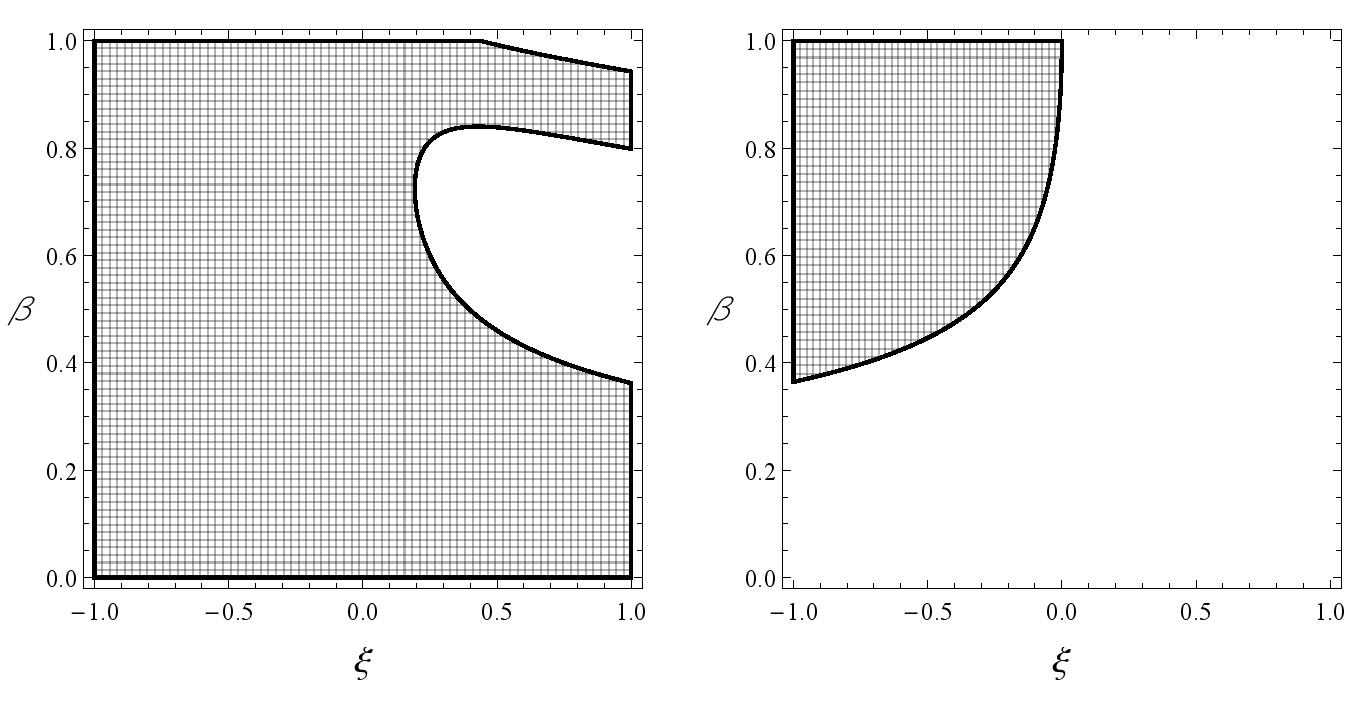
Figure 2: Points within the shaded region represent values of the $(\xi,\beta)$ space for which the vacuum polarization is negative at the event horizon (left panel). The shaded region in the right panel represents points with the property $\langle\phi^{2}\rangle_{6}\to 0^{-}$ as $r\to\infty.$

Now, let us analyze the results obtained for the $7$-dimensional black hole. At the event horizon for the conformal and minimal coupling one has

$$K\langle\phi^{2}\rangle_{7} = \frac{f^{\prime\prime}}{192r_{+}^{4}}-\frac{7{f^{\prime\prime}}^{2}}{2304r_{+}^{2}}-\frac{653{f^{\prime\prime}}^{3}}{2903040}-\frac{f^{\prime}}{32r_{+}^{5}}-\frac{13{f^{\prime}}^{2}}{1728r_{+}^{4}}-\frac{221{f^{\prime}}^{3}}{72576r_{+}^{3}}-\frac{f^{(4)}{f^{\prime}}^{2}}{5040}-\frac{f^{(3)}f^{\prime}}{864r_{+}^{2}}$$ (43)

$$-\frac{23f^{(3)}{f^{\prime}}^{2}}{4032r_{+}}+\frac{47f^{\prime}f^{\prime\prime}}{1728r_{+}^{3}}-\frac{139{f^{\prime}}^{2}f^{\prime\prime}}{16128r_{+}^{2}}-\frac{37f^{\prime}{f^{\prime\prime}}^{2}}{96768r_{+}}+\frac{191f^{(3)}f^{\prime}f^{\prime\prime}}{120960}-\frac{13}{1296r_{+}^{6}}$$

and

$$K\langle\phi^{2}\rangle_{7} = -\frac{8f^{\prime\prime}}{9r_{+}^{4}}+\frac{{f^{\prime\prime}}^{2}}{18r_{+}^{2}}-\frac{1}{630}{f^{\prime\prime}}^{3}-\frac{112f^{\prime}}{9r_{+}^{5}}+\frac{199{f^{\prime}}^{2}}{36r_{+}^{4}}+\frac{19{f^{\prime}}^{3}}{126r_{+}^{3}}-\frac{1}{140}f^{(4)}{f^{\prime}}^{2}$$ (44)

$$-\frac{f^{(3)}f^{\prime}}{9r_{+}^{2}}-\frac{2f^{(3)}{f^{\prime}}^{2}}{63r_{+}}-\frac{f^{\prime}f^{\prime\prime}}{6r_{+}^{3}}+\frac{97{f^{\prime}}^{2}f^{\prime\prime}}{336r_{+}^{2}}+\frac{f^{\prime}{f^{\prime\prime}}^{2}}{126r_{+}}+\frac{1}{210}f^{(3)}f^{\prime}f^{\prime\prime}+\frac{16}{3r_{+}^{6}},$$

respectively. On the other hand, the vacuum polarization for the extremal and ultraextremal black hole is given by

$$K\langle\phi^{2}\rangle_{7} = -\frac{8f^{\prime\prime}}{9r_{\pm}^{4}}+\frac{{f^{\prime\prime}}^{2}}{18r_{\pm}^{2}}-\frac{1}{630}{f^{\prime\prime}}^{3}+\frac{16}{3r_{\pm}^{6}}+\frac{\xi^{3}\left(r_{\pm}^{2}f^{\prime\prime}-20\right)^{3}}{6r_{\pm}^{6}}-\frac{\xi^{2}\left(r_{\pm}^{2}f^{\prime\prime}-20\right)^{3}}{12r_{\pm}^{6}}$$ (45)

$$+\frac{\xi\left(3r_{\pm}^{4}{f^{\prime\prime}}^{2}-100r_{\pm}^{2}f^{\prime\prime}+960\right)\left(r_{\pm}^{2}f^{\prime\prime}-20\right)}{180r_{\pm}^{6}}$$

and

$$K\langle\phi^{2}\rangle_{7}=-\frac{16(5\xi-1)^{2}(10\xi-1)}{3r^{6}}.$$ (46)

And finally the result for the electrically charged Tangherlini black hole is

$$\langle\phi^{2}\rangle_{7} = \frac{1}{r_{+}^{6}}\left[\frac{1}{x^{14}}\left(\frac{360\beta^{8}}{7}-144\beta^{4}+1152\beta^{4}\xi+\frac{360}{7}\right)+\frac{24\eta}{x^{18}}\left(\frac{109\beta^{4}}{7}-232\beta^{4}\xi-\frac{22}{7}-\frac{22\beta^{8}}{7}\right)\right.$$

$$+\frac{\beta^{4}}{x^{22}}\left(-\frac{940\beta^{8}}{7}-\frac{49688\beta^{4}}{63}+2640\beta^{4}\xi^{2}+5160\beta^{8}\xi+\frac{60944\beta^{4}\xi}{3}+5160\xi-\frac{940}{7}\right)$$

$$\left.+\frac{\eta\beta^{8}}{x^{26}}\left(-3600\xi^{2}-\frac{48400\xi}{3}+\frac{1240}{3}\right)+\frac{\beta^{12}}{x^{30}}\left(288\xi^{3}+4416\xi^{2}+\frac{175072\xi}{15}-\frac{60544}{315}\right)\right],$$

where $\eta=1+\beta^{4}.$ The sign of the vacuum polarization at the event horizon as well as its asymptotic behavior as $r\to\infty$ is shown in Fig. 3. A more close examination shows that the vacuum polarization at the event horizon is always negative for the minimal coupling, whereas for the conformal coupling it is positive for $0.697<\xi<0.825.$ Note qualitative similarity of the results presented in Fig 2 to Fig. 3.

Figure 3: Points within the shaded region represent values of the $(\xi,\beta)$ space for which the vacuum polarization is negative at the event horizon (left panel). The shaded region in the right panel represents points with the property $\langle\phi^{2}\rangle_{7}\to 0^{-}$ as $r\to\infty.$

Finally, we remark that the vacuum polarization on the degenerate horizon of the extremal black hole can easily be calculated using the line element (7) describing the spacetimes with the maximally symmetric subspaces. Because of the symmetries this approach is especially useful for the higher-dimensional black holes.

II.3 Trace of the stress-energy tensor of the conformally coupled massive fields

The one-loop effective action constructed from the Green function (12) is given by

$$W^{(1)}=\int d^{D}x(-g)^{1/2}{\cal L},$$ (48)

where

$${\cal L}=\frac{1}{2(4\pi)^{D/2}}\sum_{k=\lfloor\frac{D}{2}\rfloor+1}^{N}\frac{a_{k}}{(m^{2})^{k-D/2}}\Gamma(k-\frac{D}{2}),$$ (49)

and the stress-energy tensor can be calculated using the standard formula

$$T^{ab}=\frac{2}{(-g)^{1/2}}\frac{\delta}{\delta g_{ab}}W^{(1)}.$$ (50)

It should be noted that the total divergences that are present in the effective action can be discarded. For example, when calculating the stress-energy tensor in $D=4$ and $D=5$ the number of the curvature invariants can be reduced from 28 to 10.

For the conformally coupled fields one has interesting relations between the trace of the stress-energy tensor and the field fluctuation. Indeed, provided $\xi=(D-2)/(4D-4),$ we have

$$\langle T_{a}^{a}\rangle_{D}=\begin{cases}\mathfrak{C}_{D}-m^{2}\langle\phi^{2}\rangle_{D}&\text{for $D$-even}\\ \frac{1}{2}m\mathfrak{C}_{D}-m^{2}\langle\phi^{2}\rangle_{D}&\text{for $D$-odd},\end{cases}$$ (51)

where $\mathfrak{C}_{D}$ is given by

$$\mathfrak{C}_{D}=\frac{a_{\lfloor D/2\rfloor}}{(4\pi)^{\lfloor D/2\rfloor}}.$$ (52)

For the Schwinger-DeWitt expansion the first-order term cancels with the “anomalous term” and the next to leading term is precisely the first-order approximation to the trace. Similarly, the next-to leading term of the trace is equal to the next-to-next-to leading term of the vacuum polarization $\langle\phi^{2}\rangle_{D}.$ It should be noted that although the calculation of the trace of the stress-energy with the aid of Eq. (51) requires prior knowledge of the next-to-leading terms of the field fluctuation (which are expressed in terms of the Hadamard-DeWitt coefficients), it is still much more simple than the computations of the functional derivatives of the action with respect to the metric tensor. Moreover, it can be regarded as a useful check of the calculations.

Using (50) we have constructed the stress-energy tensor of the massive quantized fields in $4\leq D\leq 7$ for the general static and spherically-symmetric spacetime.Additionally, for $D=4$ and 5 we have also calculated the next-to-leading terms. On the other hand, we have calculated the first three terms of the expansion of the field fluctuation in $D=4$ and $D=5$ and the first two terms in $D=6$ and $D=7$ and checked the validity of Eq. (51) for the general static and spherically-symmetric metric. Since the final results are complicated and not very illuminating, here we present only the trace of the stress-energy tensor in the spacetime of the Tangherlini black hole. Regardless of the adapted method, after some algebra, one has

$$\langle T_{a}^{a}\rangle_{4}=-\frac{r_{+}^{2}(81r-97r_{+})}{4032\pi^{2}m^{2}r^{9}}-\frac{r_{+}^{2}\left(420r^{2}-1125rr_{+}+727r_{+}^{2}\right)}{2100\pi^{2}m^{4},r^{12}}$$ (53)

$$\langle T_{a}^{a}\rangle_{5}=-\frac{r_{+}^{4}\left(243r^{2}-323r_{+}^{2}\right)}{5040\pi^{2}mr^{12}}-\frac{r_{+}^{4}\left(1152r^{4}-3704r^{2}r_{+}^{2}+2727r_{+}^{4}\right)}{2240\pi^{2}m^{3}r^{16}},$$ (54)

$$\langle T_{a}^{a}\rangle_{6}=-\frac{r_{+}^{6}\left(22680r^{6}-81970r^{3}r_{+}^{3}+65041r_{+}^{6}\right)}{10080\pi^{3}m^{2}r^{20}}$$ (55)

and

$$\langle T_{a}^{a}\rangle_{7}=-\frac{r_{+}^{8}\left(320r^{8}-1256r^{4}r_{+}^{4}+1047r_{+}^{8}\right)}{128\pi^{3}mr^{24}}.$$ (56)

III Final remarks

The Schwinger-DeWitt method gives unique possibility to study the quantum effects in various dimensions. Moreover, as the sole criterion for its applicability is demanding that the Compton length associated with the field be small the with respect to the characteristic radius of the curvature of the background geometry, the Schwinger-DeWitt approach is also quite robust. In practice, it turns out that the reasonable results can be obtained for $Mm>2$, where $M$ is the mass of the black hole Taylor et al. (2000). A comparison made in Refs. Breen and Ottewill (2010); Thompson and Lemos (2009) between the numerical and analytical results confirms accuracy of the Schwinger-DeWitt method.

In this paper, using the generalized Schwinger-DeWitt approach, we have calculated the vacuum polarization effects of the quantized massive scalar field in the spacetime of the $D$-dimensional $(4\leq D\leq 7)$ static and spherically-symmetric black hole. A special emphasis has been put on the charged Tangherlini solutions. Contrary to the simplest Reissner-Nordström case, the vacuum polarization for the charged Tangherlini black hole depends on $\xi$ and a ratio $r_{-}/r_{+}$ in a quite complicated way, as expected. Our results can also be used to construct $\langle\phi^{2}\rangle$ when a cosmological constant is present, as, for example, in a spacetime of the lukewarm black hole. They can be generalized to the case of topological black holes.

Since the geometry of the closest vicinity of the extremal black hole is a direct product of the two maximally symmetric spaces $AdS_{2}\times S^{D-2}$ it is possible to calculate $\langle\phi^{2}\rangle_{D}$ at the degenerate horizon without referring to the black hole metric. Because of massive simplifications in the product space, the thus constructed result is relatively simple to obtain and may serve as an important check of the calculations.

For the conformally coupled field we have investigated the relation between the trace of the stress-energy tensor and the vacuum polarization. It should be emphasized that the calculation of the trace from the vacuum polarization is far more efficient than the calculations of the trace from the stress-energy tensor, even though the next-to-leading terms of the approximation of $\langle\phi^{2}\rangle_{D}$ are needed.

Finally, we briefly describe our calculational strategy. First, we have constructed the Hadamard-DeWitt coefficients for a general $D$-dimensional metric (2). The hard part of the calculations has been carried out using FORM Vermaseren (2000) (a well-known program in high-energy physics), whereas massive simplifications have been performed in MATHEMATICA. Further, the functional derivatives of the general effective action (constructed from the complicated algebraic and differential curvature invariants) with respect to the metric tensor tensor have been calculated using fast FORM code. The results have been checked against the analogous results obtained from the time and radial Euler-Lagrange equations. The remaining independent component of the stress-energy tensor has been constructed with the aid of the covariant conservation equation.

*

Appendix A The general results

In this appenedix we present in a tabular form our general results for the massive quantized field in the spacetime of the static and spherically symmetric black holes. Making use of the formulas (19) and (36) and the informations contained in the tables the vacuum polarization $\langle\phi^{2}\rangle_{D}$ can easily be reconstructed.

		$D=4$			$D=5$
$k$	$F_{k}(r)$	$\alpha_{k}^{0}$	$\alpha_{k}^{1}$	$\alpha_{k}^{2}$	$\alpha_{k}^{0}$	$\alpha_{k}^{1}$	$\alpha_{k}^{2}$
1	$\dfrac{1}{r^{4}}$	1/15	-2/3	2	1/2	-6	18
2	$\dfrac{f}{r^{4}}$	0	2/3	-4	-1	12	-36
3	$\dfrac{f^{2}}{r^{4}}$	-1/15	0	2	1/2	-6	18
4	$\dfrac{f^{\prime}}{r^{3}}$	-1/3	10/3	-8	-4/3	14	-36
5	$\dfrac{ff^{\prime}}{r^{3}}$	7/15	-4	8	26/15	-16	36
6	$\dfrac{f^{\prime 2}}{r^{2}}$	13/45	-3	8	59/120	-6	18
7	$\dfrac{f^{\prime\prime}}{r^{2}}$	-1/18	2/3	-2	-1/6	2	-6
8	$\dfrac{ff^{\prime\prime}}{r^{2}}$	-1/90	-1/3	2	-7/30	0	6
9	$\dfrac{f^{\prime}f^{\prime\prime}}{r}$	-1/30	-2/3	4	-1/20	-1	6
10	$f^{\prime\prime 2}$	1/60	-1/6	1/2	1/60	-1/6	1/2
11	$\dfrac{ff^{(3)}}{r}$	-1/5	1	0	-3/10	3/2	0
12	$f^{(3)}f^{\prime}$	-1/30	1/6	0	-1/30	1/6	0
13	$ff^{(4)}$	-1/30	1/6	0	-1/30	1/6	0

Table 2: The functions $F_{k}(r)$ and the coefficients $\alpha_{k}^{i}$ of the massive scalar field in $(D=4)$ and $(D=5)$-dimensional static, spherically symmetric black hole.

$k$	$F_{k}(r)$	$k$	$F_{k}(r)$	$k$	$F_{k}(r)$
$1$	$\dfrac{1}{r^{6}}$	$13$	$\dfrac{f^{2}f^{\prime\prime}}{r^{4}}$	$25$	$\dfrac{f^{(3)}f^{\prime 2}}{r}$
$2$	$\dfrac{f}{r^{6}}$	$14$	$\dfrac{f^{\prime}f^{\prime\prime}}{r^{3}}$	$26$	$\dfrac{ff^{(3)}f^{\prime\prime}}{r}$
$3$	$\dfrac{f^{2}}{r^{6}}$	$15$	$\dfrac{ff^{\prime}f^{\prime\prime}}{r^{3}}$	$27$	$f^{(3)}f^{\prime}f^{\prime\prime}$
$4$	$\dfrac{f^{3}}{r^{6}}$	$16$	$\dfrac{{f^{\prime}}^{2}f^{\prime\prime}}{r^{2}}$	$28$	$f{f^{(3)}}^{2}$
$5$	$\dfrac{f^{\prime}}{r^{5}}$	$17$	$\dfrac{f^{\prime\prime 2}}{r^{2}}$	$29$	$\dfrac{ff^{(4)}}{r^{2}}$
$6$	$\dfrac{ff^{\prime}}{r^{5}}$	$18$	$\dfrac{ff^{\prime\prime 2}}{r^{2}}$	$30$	$\dfrac{f^{2}f^{(4)}}{r^{2}}$
$7$	$\dfrac{f^{2}f^{\prime}}{r^{5}}$	$19$	$\dfrac{f^{\prime}f^{\prime\prime 2}}{r}$	$31$	$\dfrac{ff^{(4)}f^{\prime}}{r}$
$8$	$\dfrac{f^{\prime 2}}{r^{4}}$	$20$	$f^{\prime\prime 3}$	$32$	$f^{(4)}f^{\prime 2}$
$9$	$\dfrac{ff^{\prime 2}}{r^{4}}$	$21$	$\dfrac{ff^{(3)}}{r^{3}}$	$33$	$ff^{(4)}f^{\prime\prime}$
$10$	$\dfrac{f^{\prime 3}}{r^{3}}$	$22$	$\dfrac{f^{2}f^{(3)}}{r^{3}}$	$34$	$\dfrac{f^{2}f^{(5)}}{r}$
$11$	$\dfrac{f^{\prime\prime}}{r^{4}}$	$23$	$\dfrac{f^{(3)}f^{\prime}}{r^{2}}$	$35$	$ff^{(5)}f^{\prime}$
$12$	$\dfrac{ff^{\prime\prime}}{r^{4}}$	$24$	$\dfrac{ff^{(3)}f^{\prime}}{r^{2}}$	$36$	$f^{2}f^{(6)}$

Table 3: The functions $F_{k}(r)$ of the quantized massive field in the spacetime of the static and spherically-symmetric black holes in $D=6$ and $7.$

$k$	$\alpha_{k}^{0}$	$\alpha_{k}^{1}$	$\alpha_{k}^{2}$	$\alpha_{k}^{3}$	$k$	$\alpha_{k}^{0}$	$\alpha_{k}^{1}$	$\alpha_{k}^{2}$	$\alpha_{k}^{3}$
1	$74/63$	-116/5	144	-288	19	2/315	-1/15	-2/3	4
2	-58/15	356/5	-432	864	20	-1/630	1/60	-1/12	1/6
3	58/15	-356/5	432	-864	21	-11/15	116/15	-20	0
4	-74/63	116/5	-144	288	22	92/105	-42/5	20	0
5	-58/15	952/15	-336	576	23	-1/15	11/15	-2	0
6	164/15	-2384/15	752	-1152	24	149/630	-229/45	56/3	0
7	-778/105	1456/15	-416	576	25	-8/315	-8/45	4/3	0
8	116/45	-204/5	216	-384	26	-4/315	-29/45	10/3	0
9	-1103/315	2224/45	-236	384	27	1/210	-1/20	1/6	0
10	-2/315	184/45	-112/3	256/3	28	1/840	-1/60	1/12	0
11	-29/90	89/15	-36	72	29	-1/15	11/15	-2	0
12	-1/45	-68/15	52	-144	30	-5/42	2/15	2	0
13	65/126	-11/5	-16	72	31	-44/315	16/45	4/3	0
14	-1/15	-44/15	36	-96	32	-1/140	1/30	0	0
15	683/315	-232/15	4	96	33	-1/420	-1/60	1/6	0
16	131/630	-64/45	-14/3	32	34	-2/35	4/15	0	0
17	1/30	-8/15	3	-6	35	-1/70	1/15	0	0
18	89/630	-109/45	7	6	36	-1/280	1/60	0	0

Table 4: The coefficients $\alpha_{k}$ of the quantized massive field in the spacetime of the static and spherically-symmetric black holes in $D=6.$

$k$	$\alpha_{k}^{0}$	$\alpha_{k}^{1}$	$\alpha_{k}^{2}$	$\alpha_{k}^{3}$	$k$	$\alpha_{k}^{0}$	$\alpha_{k}^{1}$	$\alpha_{k}^{2}$	$\alpha_{k}^{3}$
1	16/3	-320/3	2000/3	-4000/3	19	1/126	-1/12	-5/6	5
2	-64/3	1120/3	-6400/3	4000	20	-1/630	1/60	-1/12	1/6
3	80/3	-1280/3	6800/3	-4000	21	-14/9	149/9	-130/3	0
4	-32/3	160	-800	4000/3	22	793/504	-599/36	130/3	0
5	-112/9	1880/9	-3400/3	2000	23	-1/9	11/9	-10/3	0
6	104/3	-4622/9	2500	-4000	24	61/252	-68/9	30	0
7	-5843/252	1855/6	-4100/3	2000	25	-2/63	-2/9	5/3	0
8	199/36	-1697/18	1600/3	-1000	26	-1/63	-29/36	25/6	0
9	-2659/504	569/6	-1625/3	1000	27	1/210	-1/20	1/6	0
10	19/126	71/12	-200/3	500/3	28	1/840	-1/60	1/12	0
11	-8/9	148/9	-100	200	29	-1/9	11/9	-10/3	0
12	-4/3	2/9	340/3	-400	30	-115/504	13/36	10/3	0
13	803/252	-127/6	-40/3	200	31	-11/63	4/9	5/3	0
14	-1/6	-17/3	220/3	-200	32	-1/140	1/30	0	0
15	1093/252	-209/6	25	200	33	-1/420	-1/60	1/6	0
16	97/336	-53/24	-20/3	50	34	-1/14	1/3	0	0
17	1/18	-8/9	5	-10	35	-1/70	1/15	0	0
18	95/504	-23/6	35/3	10	36	-1/280	1/60	0	0

Table 5: The coefficients $\alpha_{k}$ of the quantized massive field in the spacetime of the static and spherically-symmetric black holes in $D=7.$

References

Candelas (1980)
P. Candelas,
Phys. Rev. D21,
2185 (1980).
Candelas and Howard (1984)
P. Candelas and
K. W. Howard,
Phys. Rev. D29,
1618 (1984).
Anderson (1990)
P. R. Anderson,
Phys. Rev. D41,
1152 (1990).
Frolov (1982)
V. P. Frolov,
Phys. Rev. D26,
954 (1982).
Anderson (1989)
P. R. Anderson,
Phys. Rev. D39,
3785 (1989).
Fawcett and Whiting (1981)
M. S. Fawcett and
B. F. Whiting, in
Nuffield Workshop on Quantum Structure of Space
and Time (1981), pp.
131–154.
Fawcett (1983)
M. S. Fawcett,
Commun. Math. Phys. 89,
103 (1983).
Kofman and Sahni (1983)
L. A. Kofman and
V. Sahni,
Phys. Lett. 127B,
197 (1983).
Anderson et al. (1995)
P. R. Anderson,
W. A. Hiscock,
and D. A.
Samuel, Phys. Rev.
D51, 4337 (1995).
Shiraishi (1992)
K. Shiraishi,
Mod. Phys. Lett. A7,
3569 (1992).
Quinta et al. (2016)
G. M. Quinta,
A. Flachi, and
J. P. S. Lemos,
Phys. Rev. D93,
124073 (2016).
Popov (2004)
A. A. Popov,
Phys. Rev. D70,
084047 (2004.
Flachi and Tanaka (2008)
A. Flachi and
T. Tanaka,
Phys. Rev. D78,
064011 (2008).
Tomimatsu and Koyama (2000)
A. Tomimatsu and
H. Koyama,
Phys. Rev. D61,
124010 (2000).
Koyama et al. (2000)
H. Koyama,
Y. Nambu, and
A. Tomimatsu,
Mod. Phys. Lett. A15,
815 (2000).
Matyjasek et al. (2010)
J. Matyjasek,
D. Tryniecki,
and
K. Zwierzchowska,
Phys. Rev. D81,
124047 (2010).
Popov (2016)
A. A. Popov,
Phys. Rev. D94,
124033 (2016).
Levi and Ori (2016)
A. Levi and
A. Ori,
Phys. Rev. D94,
044054 (2016).
Frolov and Garcia (1983)
V. P. Frolov and
A. Garcia,
Physics Letters A 99,
421 (1983).
Frolov and Sanchez (1986)
V. P. Frolov and
N. G. Sanchez,
Phys. Rev. D33,
1604 (1986).
Frolov et al. (1989)
V. P. Frolov,
F. D. Mazzitelli,
and J. P. Paz,
Phys. Rev. D40,
948 (1989).
Shiraishi and Maki (1994a)
K. Shiraishi and
T. Maki,
Class. Quant. Grav. 11,
695 (1994a).
Shiraishi and Maki (1994b)
K. Shiraishi and
T. Maki,
Class. Quant. Grav. 11,
1687 (1994b).
Thompson and Lemos (2009)
R. T. Thompson and
J. P. S. Lemos,
Phys. Rev. D80,
064017 (2009).
Matyjasek and Sadurski (2015)
J. Matyjasek and
P. Sadurski,
Phys. Rev. D91,
044027 (2015).
Matyjasek and Sadurski (2014)
J. Matyjasek and
P. Sadurski,
Acta Phys. Polon. B45,
2027 (2014).
Quinta et al. (2018)
G. M. Quinta,
A. Flachi, and
J. P. Lemos,
Phys. Rev. D97,
025023 (2018).
Taylor and Breen (2017)
P. Taylor and
C. Breen,
Phys. Rev. D96,
105020 (2017).
Taylor and Breen (2016)
P. Taylor and
C. Breen,
Phys. Rev. D94,
125024 (2016).
Flachi et al. (2016)
A. Flachi,
G. M. Quinta,
and J. P. S.
Lemos, Phys. Rev.
D94, 105001
(2016).
Breen et al. (2015)
C. Breen,
M. Hewitt,
A. C. Ottewill,
and
E. Winstanley,
Phys. Rev. D92,
084039 (2015).
Page (1982)
D. N. Page,
Phys. Rev. D25,
1499 (1982).
Frolov and Zelnikov (1987)
V. P. Frolov and
A. I. Zelnikov,
Phys. Rev. D35,
3031 (1987).
Frolov and Zelnikov (1984)
V. P. Frolov and
A. I. Zelnikov,
Phys. Rev. D29,
1057 (1984).
Frolov (1986)
V. P. Frolov,
Trudy Fiz. Inst. Lebedev. 169,
3 (1986).
Matyjasek (1996)
J. Matyjasek,
Phys. Rev. D53,
794 (1996).
Matyjasek (2000)
J. Matyjasek,
Phys. Rev. D61,
124019 (2000).
Matyjasek (2001)
J. Matyjasek,
Phys. Rev. D63,
084004 (2001).
Taylor et al. (2000)
B. E. Taylor,
W. A. Hiscock,
and P. R.
Anderson, Phys. Rev.
D61, 084021
(2000).
Breen and Ottewill (2010)
C. Breen and
A. C. Ottewill,
Phys. Rev. D82,
084019 (2010).
Vermaseren (2000)
J. A. M. Vermaseren
(2000), eprint math-ph/0010025.
*