The (small) vibrations of thin plates
In memory of Stephen A. Andrea

Abstract.

We describe the equations of motion of elastodynamic bounded bodies in 3-space, and their linearizations at a stationary point. Using the latter as an approximation to model small motions, we develop a scheme to find numerical solutions of these equations. We discretize the solution in the space of PL vector fields associated to the oriented faces of the first barycentric subdivision of a given smooth initial triangulation of the body, in order to exploit the algebraic topology properties of the body that these vector fields encode into the sought after solution, and solve a weak version of the linearized equations in that context. We apply our scheme to a couple of relevant examples of thin bodies, bodies where one of the dimensions is at least one order of magnitude in size less than the other two, and determine numerical approximations to some of their resonance modes of vibration. The results obtained are consistent with known vibration patterns for these bodies derived experimentally.

1. Introduction

It is a classical experimental result to obtain the normal modes of vibrations of an unassembled violin plate by horizontally mounting the plate with its belly down, sprinkling the other side with a fine powder, and causing the plate to vibrate by applying an external sinusoidal pressure force that points in the vertical direction, and that hits the belly of the mounted plate straight up. At certain frequencies resonance occurs, and the vibration of the plate bounces the powder into the nonvibrating nodal areas, outlining the nodal and antinodal configurations of the plate at its eigenfrequency modes. This experiment goes as far back as Félix Savart in 1830, building on a method developed by Ernst Chladni, (see, for instance, [15, $2^{\rm nd}$ column, page 171]; this reference describes various other types of acoustic experiments also). Today, the nodal lines of the plate vibrating at these frequencies are called the Chladni lines, and the entire portrait that they make is called the Chladni pattern.

In this article we study the theoretical underpinning of these experiments. We consider the plate material as an incompressible orthotropic elastic Hooke body, whose stored energy function is characterized by nine independent elastic constant parameters. With the density as an additional parameter, we describe the equations of motion governing the time evolution of these bodies, and concentrate our attention on solving these equations numerically. We then use these solutions to describe the Chladni patterns of the vibrating violin plate, and more generally, the Chladni patterns of very thin plates.

The Cauchy problem for the equations of motion of an incompressible elastic coercive body whose boundary is free to move is well-posed, at least for a short time [10, 11], and the derivation of numerical solutions to it is a matter of interest in its own right. This is a difficult problem, essentially because the nonlinearity of the equation of motion being solved is of a pseudodifferential nature, with changes to the solution in a neighborhood of any point affecting the solution everywhere else, all at once, since the solution of the pressure equation depends on global conditions across the body.

We solve these difficulties in two steps: The first is to use discretizing spaces for the solution that we seek that have encoded into them the algebraic topology of divergence-free fields. Such a condition, a matter of satisfying an equation that locally involves finitely many of the coefficients in the discretized unknown, is then left to be regulated by the equation itself, and if holding initially, it should be satisfied at later times within a small margin of error also due to the well-posedness of the problem we solve, thus ensuring that the nonlocal incompressible condition holds in time. The discretizing spaces used are associated to the dual of the Whitney forms of an oriented triangulation of the body, which in dimension three leads to a simplicial complex with functions as complex groups in degrees zero, and three, and vector fields in degrees one, and two, respectively, whose cohomology is the cohomology of the body, and which in degree two have as cycles the Abelian group of divergence-free vector fields where the actual solutions to the equations of motion lie; the second step arises by observing that the Chladni patters must involve primarily the small vibrations of the bodies under consideration, and these can be approximated well by the solution to the linearized equations of motion about the canonical stationary state. Under that assumption, which we follow, we can tame the effects of the almost degenerate nature of the bodies, bounded three dimensional with one of its directions at least one order of magnitude smaller in length than the other two, by choosing the simplices in the triangulation to be nondegenerate, and using sufficiently many of them so that the weak formulation of the problem that we solve in our numerical scheme captures well the vibrations of the body at any point. The solution so obtained feels the contributions to the vibration modes arising from all of the points, including the many far apart boundary points that are separated by a very small distance within the body. It does so, however, at a very large computational memory expense, a consequence of the need to triangulate the body with the appropriate resolution in order to derive accurate results.

The large systems of equations that need to be solved, however sparse, are computationally challenging, and this is a difficulty that we must face even after resolving that of determining the systems themselves. The judicious choice of discretizing spaces minimizes these difficulties. Since we encode in them the initial conditions of the waves we seek, with the algebraic topological properties that they have, we can then allow the well-posedness of the equations solved for to play its role in keeping the numerical solutions derived physically accurate in time.

The way the various types of waves propagate within the body is a property encoded in the density and elastic constants parameters that are part of the equations of motion. We may think of the body as an ensemble of springs, one per every pair of faces in the triangulation whose stars intercept nontrivally, placed within the body according to the orientation of the said faces. The waves within the body, Lamb, Rayleigh, shear, or otherwise, result from the interaction of the elements of this ensemble of springs as they move, which is ruled by the equations of motion. They all fit now within a single framework. And the solutions we construct numerically to describe these waves are built to maintain the global topological constraint imposed by the incompressibility condition in time, yielding very accurate approximations to the actual motion of the body. The innovative use of our discretizing spaces counterbalances the need to go through the computational complexities inherent in the problem, in exchange for producing results that are faithful to the physical reality of the motion while in the elastic regime.

Although here we apply our approach to orthotropic bodies only, the same could be done to study the vibrations of elastic bodies in general, as long as their stored energy function is (or is assumed to be) smooth. The variational principle used to derive the equations of motion can be extended to treat cases where part of the boundary is fixed, while the rest is free to move, and so, for instance, we could treat the problem of isotropic functionally graded plates [16, 2] in a way that is far easier by comparison with the problems analyzed here, given the much smaller number of elastic constant parameters even if their values now vary across the body. The resulting simulations would be computationally more complex than approaches describing the motion in terms of an ad hoc small number of degrees of freedom, and basic assumptions, but the physical meaning of the results would be unquestioned.

The simulations we carry out fit well with the classical experiments on violin plates, and serve also in the study of small vibrations of thin plates in general, as observed above. They can be used to solve problems of practical importance. For assuming given a set of parameters determining the elastodynamic properties of the material being used in making the thin plate, and a desired Chladni pattern, we may find the geometry of the plate that conforms to that pattern. This gives an idea on how to carve the material in order to achieve a specified vibration pattern, or how this pattern is affected when the elastodynamic constants of the material vary across it, for instance, the material that results by coating with a protective layer of varnish a given plate of wood. We can find the natural vibration pattern of a sheet made of aluminum, and study how that will change when instead we use an alloy of aluminum and copper to make the sheet with a material whose strength is larger. In fact, given the elastic constants of the material at room temperature, we should be able to determine the natural free and dampening vibration modes of a pointy thin cylindrical shell made out of this material when accelerating in open space, and improve on the result significantly if we take into consideration the rising temperature of the accelerating shell that is due to dampening modes, and consider its effect on the elastic constants of the material used to make it as time passes by, again producing results that are based on the fundamental physical principles ruling the motion.

1.1. Organization of the article

In §2 we state the equations of motion of incompressible elastodynamic bodies, and briefly sketch the proof of the well-posedness of its Cauchy problem in $C^{k,\alpha}$ spaces, spaces which are better suited for our purpose here than the Sobolev spaces used in the original proof [10, 11]. We derive also the specific linearization of these equations that we wish to solve numerically here, with its natural set of boundary conditions. In §3, we define the generalized Hooke materials, among which are the orthotropic ones that we use, and after recalling the general notions of stress and strain tensors. For the sake of completeness, we recall also the definition of the elastic parameters that characterize their stored energy functions, and the data for the material that we shall use in our numeric simulations in §5 below. In §4, we write down the algorithms that we use to solve the said equation of §2, after a careful discussion of the discretizing spaces, closely related to the divergence-free vector fields that represent cohomology classes of the body in degree two, and which we describe using the metric dual of the Whitney forms associated to the faces of the first barycentric subdivision of a given triangulation. We emphasize the appropriateness of this choice by describing the metric dual simplicial complex of the usual de Rham complex, all of whose Abelian groups of chains can be expressed in terms of the metric duals of the Whitney forms of various degrees, and show how the divergence-free vector fields appear as the group of cycles of this complex in degree two. In §5, we present the various simulations that we have carried out, as well as some additional numerical computations to support the virtues of our approach. We end with some remarks in §6, where among other things, we observe that the solution to the linearized equations of motion, which we study here as approximations to small vibrations of the body, is essentially the initial step in a Newton iteration scheme to solve the actual equations of motion, at least on the time interval where they do not develop singularities (if at all).

2. The equations of motion

In this section, we begin by recalling the equations of motion of an elastodynamic body, and their linearization. We refer the reader to [10, 11] for details.

Let us suppose that $\Omega$ is a bounded domain in ${\mathbb{R}}^{3}$. We assume its boundary to be of class $C^{1,\alpha}$, and that the density $\rho$ of the material filling $\Omega$ is constant.

The motion of $\Omega$ is encoded into a curve

$$\eta(t):\Omega\hookrightarrow{\mathbb{R}}^{3}$$

of embeddings of $\Omega$ into ${\mathbb{R}}^{3}$ that preserve volume. The path $t\rightarrow\eta(t)(x)$ denotes the position at time $t$ of a particle initially at $x\in\Omega$, and if $D\eta(t)(x)=(\partial_{x^{i}}\eta^{j}(t)(x))$ is the deformation gradient, the volume preserving property or incompressibility, is equivalent to

(1) $$J(\eta(t))=\det{D\eta(t)(x)}=1\,.$$

The material properties of $\Omega$ are characterized by its stored energy function $W$. This function indicates how the various particles of $\Omega$ are bound to each other, and it is often assumed to be a function of the deformation gradient, $W=W(D\eta)$. A typical choice is that given by $W(\partial_{i}\eta^{j})={\displaystyle-\frac{3}{2}+\frac{1}{2}}\partial_{i}\eta^{\alpha}\partial_{i}\eta^{\alpha}$ which models isotropic neoHooke materials (throughout the paper we use the standard convention of adding over repeated indexes). For the time being, we keep a general point of view in mind.

In the presence of no external forces, the trajectory of the body will be an extremal path of the Lagrangian

$${{\mathcal{L}}}(\eta)=\frac{1}{2}\int_{0}^{T}\int_{\Omega}\rho\|\dot{\eta}(t)(x)\|^{2}dxdt-\int_{0}^{T}\int_{\Omega}W(\partial_{i}\eta^{\alpha}(t)(x))dxdt\;.$$

The stationary points of ${\mathcal{L}}(\eta)$ must be searched for among variations of $\eta(t)$ preserving (1). If we let $\eta(t,s)$ be one such variation, and define $\zeta:\eta(t)(\Omega)\rightarrow{\mathbb{R}}^{3}$ by

$$\zeta(\eta(t)(x))=\partial_{s}\eta(t,s)\mid_{s=0}(x)\,,$$

we then have that ${\rm div}\,\zeta=\partial_{x^{j}}\zeta^{j}=0$, and

$$\begin{array}[]{rcl}{\displaystyle\frac{d}{ds}{\mathcal{L}}(\eta(t,s))\mid_{s=0}}&=&{\displaystyle\int_{0}^{T}\int_{\Omega}\langle(-\rho\ddot{\eta}+{\rm Div}W^{{}^{\prime}}(D\eta))(x),\zeta(\eta(t)(x)\rangle dxdt}\\ &&{\displaystyle\;\;\;-\int_{0}^{T}\int_{\partial\Omega}\langle W^{{}^{\prime}}(D\eta)N,\zeta(\eta(t)(x))\rangle d\sigma dt}\;,\end{array}$$

where $W^{{}^{\prime}}$ means the derivative of $W$ with respect to the variables $D\eta$, ${\rm Div}$ is the divergence of $W^{{}^{\prime}}$ with respect to the material coordinates $x$, $N$ is the unit normal to $\partial\Omega$ and $d\sigma$ is the surface measure for $\partial\Omega$. It thus follows that the motion of the body takes place along a solution of the free boundary value problem

(2) $$\rho\ddot{\eta}(t)(x)-{\rm Div}\,W^{{}^{\prime}}(D\eta(t)(x))=\nabla p(t)(\eta(t)(x))\,,$$

(3) $$W^{{}^{\prime}}(D\eta)N+p(t)(\eta(t)(x))J^{b}(\eta)\nu\circ\eta=0\;{\rm on}\;\partial\Omega\,,$$

for a certain function $p(t):\eta(t)(\Omega)\rightarrow{\mathbb{R}}$. Here, $J^{b}(\eta(t))$ is the Jacobian determinant of $\eta(t)$ restricted to the boundary $\partial\Omega$, and $\nu:\partial(\eta(t)(\Omega))\rightarrow{\mathbb{R}}^{3}$ is the unit normal.

In coordinates $\eta^{\alpha}=\eta^{\alpha}(x^{1},x^{2},x^{3})$, we have that

$$({\rm Div}\,W^{{}^{\prime}})^{\alpha}=\partial_{x^{i}}\left(\frac{\partial W}{\partial(\partial_{i}\eta^{\alpha})}\right)\stackrel{{\scriptstyle{\rm def}}}{{=}}A_{ij}^{\alpha\beta}(D\eta)\partial_{i}\partial_{j}\eta^{\beta}$$

and

$$(W^{{}^{\prime}}(D\eta)N)^{\alpha}=\frac{\partial W}{\partial(\partial_{i}\eta^{\alpha})}N^{i}\,,$$

respectively, and the system above is given by

$$\rho\ddot{\eta}^{\alpha}=A_{ij}^{\alpha\beta}(D\eta)\partial_{i}\partial_{j}\eta^{\beta}+(\partial_{\alpha}(p(t)))\circ\eta\,,$$

$$\frac{\partial W}{\partial(\partial_{i}\eta^{\alpha})}N^{i}+p(t)(\eta(t)(x))J^{b}(\eta)(\nu\circ\eta)^{\alpha}=0\,.$$

We require that the stored energy function $W$ be coercive at least for small vibrations. That is to say, we require the operator $A_{ij}^{\alpha\beta}(D\eta)\partial_{i}\partial_{j}$ to be uniformly elliptic in a neighborhood of the stationary curve $\eta(t)(x)=x$.

Equations (1), (2), (3) are the equations of motion of an incompressible elastic body of stored energy $W$.

Given an operator $F$, we define the operator $F_{\eta}$ by $F_{\eta}u=(F(u\circ\eta^{-1}))\circ\eta$. If we now differentiate (1) with respect to $t$, we obtain that ${\rm div}_{\eta}\dot{\eta}=0$, and upon a second differentiation, we have that

$${\rm div}_{\eta}\ddot{\eta}=-[(\dot{\eta}\circ\eta^{-1}\cdot\nabla,{\rm div}]_{\eta}\dot{\eta}={\rm trace}(D_{\eta}\dot{\eta})^{2}\,.$$

We use this result to express equations (1), (2), (3) as a first order system.

Proposition 1.

Let $\eta(t)$ be a curves of embeddings describing the motions of an incompressible elastic body of constant density $\rho$ and stored energy function $W$. Then ${\rm div}_{\eta}\dot{\eta}=0$, the vector $W^{\prime}(D\eta)N$ is perpendicular to $W^{\prime}(D\eta)T$ (where $T$ is any vector tangent to $\partial\Omega$), and

(4) $$\frac{d}{dt}\left(\begin{array}[]{c}\eta\\ \rho\dot{\eta}\end{array}\right)=\left(\begin{array}[]{c}\dot{\eta}\\ A(\eta,\dot{\eta})\end{array}\right)\stackrel{{\scriptstyle{\rm def}}}{{=}}F(\eta,\dot{\eta})\;,$$

where

$$A(\eta,\dot{\eta})={\rm Div}\,W^{\prime}(D\eta)+\nabla_{\eta}q\,,$$

and $q$ solves the boundary value problem

(5) $$\begin{array}[]{c@{=}l}\Delta_{\eta}q&\;-{\rm div}_{\eta}{\rm Div}\,W^{\prime}(D\eta)+\rho\,{\rm trace}(D_{\eta}\dot{\eta})^{2}\vspace{1mm}\\ q\mid_{\partial\Omega}&\;-{\displaystyle\frac{\langle W^{\prime}(D\eta)N,\nu\circ\eta\rangle}{J^{b}(\eta)}}\;.\end{array}$$

Here, $q=p\circ\eta$ where $p$ is as in $(\ref{eq2})$, $N$ and $\nu$ are the unit vectors normal to $\partial\Omega$ and $\partial(\eta(t)(\Omega))$, respectively, and $J^{b}(\eta)$ is the Jacobian determinant of $\eta$ restricted to the boundary.

The function $q$ is normally called the pressure.

Since $W$ is coercive, the boundary value problem (5) is elliptic, and has a unique pressure function solution $q=q(\eta,\dot{\eta})$. This solution is a nonlocal pseudodifferential operator in $(\eta,\dot{\eta})$. The system (4) admits the time independent curve $\eta={\mathchoice{\rm 1\mskip-4.0mul}{\rm 1\mskip-4.0mul}{\rm 1\mskip-4.5mul}{\rm 1\mskip-5.0mul}}$ as a solution, with pressure function the constant $q=-\langle W^{\prime}({\mathchoice{\rm 1\mskip-4.0mul}{\rm 1\mskip-4.0mul}{\rm 1\mskip-4.5mul}{\rm 1\mskip-5.0mul}})N,N\rangle$.

For reasonably smooth $\Omega$ and coercive stored energy function $W$, the Cauchy problem for (4) with initial condition $(\eta(0),\dot{\eta}(0))=({\mathchoice{\rm 1\mskip-4.0mul}{\rm 1\mskip-4.0mul}{\rm 1\mskip-4.5mul}{\rm 1\mskip-5.0mul}},w)$, $w$ a divergence-free vector field, is well-posed. This was proven in [11] working on Sobolev spaces. With some additional difficulties, the same argument employed there can be cast working over $C^{k,\alpha}$-spaces instead; we just need to invoke the continuity of pseudodifferential operators on these spaces, as opposed to that on Sobolev spaces, and redo the said argument in this new context. The benefit of doing so is twofold: on the one hand, $C^{k,\alpha}$-spaces are better suited to analyze the question of consistency of the numerical solutions of the equations we derive in this article, and for which we use the PL vector fields associated to the elements of a triangulation as discretizing spaces; on the other hand, we get optimal regularity results for the analysis of the Cauchy problem, which can be started if we assume merely that $\eta(t)$ is a $C^{2,\alpha}$ curve of embeddings. It is for this reason that we discuss the continuity properties of $F(\eta,\dot{\eta})$ over these other spaces, as opposed to those employed in [10, 11].

Let $C^{k,\alpha}(\Omega;{\mathbb{R}}^{3})$ be the space of vector fields with $C^{k,\alpha}$-regularity. These spaces are closed under multiplication by scalar valued functions in $C^{k,\alpha}$, and pseudodifferential operators of order $n$ act continuously from $C^{k,\alpha}$ into $C^{k-n,\alpha}$ [19]. We define ${\mathcal{C}}_{k,\alpha}=C^{k,\alpha}(\Omega;{\mathbb{R}}^{3})\oplus C^{k-1,\alpha}(\Omega;{\mathbb{R}}^{3})$, and view $F$ in (4) as a map:

(6) $$\begin{array}[]{cccl}F:&{\mathcal{C}}_{k+1,\alpha}&\longrightarrow&{\mathcal{C}}_{k,\alpha}\\ &(\eta,\dot{\eta})&\longrightarrow&F(\eta,\dot{\eta})\end{array}\;.$$

In order to preserve the validity of the variational principle producing the equations of motion as a duality pairing, it is natural to impose the restriction that $k\geq 0$. We see below that the stricter assumption $k\geq 1$ is required in order to make classic sense of other terms. We shall assume the latter always.

The continuity of $F$ is a question of continuity of the map $A$ from ${\mathcal{C}}_{k+1,\alpha}$ to $C^{k-1,\alpha}(\Omega;{\mathbb{R}}^{3})$. Thus, if $(\eta,\dot{\eta})\in{\mathcal{C}}_{k+1,\alpha}$, the pressure function $q$ obtained by solving (5) must be in $C^{k,\alpha}(\Omega)$. If $\eta$ is a $C^{k+1,\alpha}$-diffeomorphism from $\Omega$ to $\eta(\Omega)$, $\dot{\eta}\in C^{k,\alpha}(\Omega;{\mathbb{R}}^{3})$, as $k\geq 1$, we have that $-{\rm div}_{\eta}{\rm Div}\,W^{\prime}(D\eta)+{\rm trace}(D_{\eta}\dot{\eta})^{2}$ is a well-defined distribution in $C^{k-2,\alpha}(\Omega)$. Since the boundary condition for $q$ lies in $C^{k,\alpha}(\partial\Omega)$, the regularity of solutions to the Dirichlet problem implies that $q$ is in $C^{k,\alpha}$, as desired.

Theorem 2.

([11, Theorem 5.53 and §6]) Let $\Omega$ be an incompressible elastic body of constant density $\rho$ and coercive stored energy function $W$. Given an initial condition $(\eta(0),\dot{\eta}(0))=({\mathchoice{\rm 1\mskip-4.0mul}{\rm 1\mskip-4.0mul}{\rm 1\mskip-4.5mul}{\rm 1\mskip-5.0mul}},w)$, $w\in C^{k,\alpha}(\Omega;{\mathbb{R}}^{3})$, $k\geq 1$, ${\rm div}\,w=0$, there exists a positive real number $T$ such that the initial value problem for (1), (2), (3) has a unique solution $\eta(t)\in C^{2}([0,T];C^{k+1,\alpha}(\Omega,{\mathbb{R}}^{3}))$ with the said initial condition. The value of $T$ depends upon the norm of finitely many derivatives of $w$ only, and the solution $\eta(t)$ is a continuous function of the initial data.

Our interest is in the motion of the bodies when they experience relatively small deformations from the stationary solution $\eta(t)(x)=x$. We shall study numerically the time evolution of the solutions to the linearized equations about $\eta(t)(x)=x$, and use them as actual approximations to the nonlinear small vibrating motions. We end this section by outlining the important details of the derivation of this linearization. (The derivation in [10, Proposition 2.8] was carried out for neoHooke materials only.) We linearize first about a fixed but arbitrary element $(\eta,\dot{\eta})$ of ${\mathcal{C}}_{k+1,\alpha}$ whose first component is a diffeomorphism onto its image, and then apply the result at the said stationary point.

We begin by linearizing the boundary condition (3), which is required in computing the linearization of the operator $F$ in (4). We fix $x\in\partial\Omega$, and pick $\{T_{1},T_{2}\}$ orthonormal and tangent to $\partial\Omega$ at $x$. We fix also the coordinates in ${\mathbb{R}}^{3}$ so that $\partial_{T_{i}}\eta\in{\mathbb{R}}^{2}\subseteq{\mathbb{R}}^{3}$ for $i=1,2$. Then,

$$(J^{b}(\eta)\nu\circ\eta)(x)=\det{\left(\begin{array}[]{c}\partial_{T_{1}}\eta\\ \partial_{T_{2}}\eta\end{array}\right)}(0,0,1)\,.$$

We let $\eta(s)=\eta+su$ and $\dot{\eta}(s)=\dot{\eta}+sv$ be the variations of $\eta$ and $\dot{\eta}$ in the directions of $u$ and $v$, respectively. Then,

(7) $$\langle\partial_{s}(J^{b}(\eta)\nu\circ\eta),\nu\circ\eta\rangle\mid_{s=0}=\\ J^{b}(\eta)\left[\det{\left(\begin{array}[]{c}\partial_{T_{1}}u\\ \partial_{T_{2}}\eta\end{array}\right)}+\det{\left(\begin{array}[]{c}\partial_{T_{1}}\eta\\ \partial_{T_{2}}u\end{array}\right)}\right]\,.$$

This is a function on $\partial\Omega$. Notice that the vector $\partial_{s}(J^{b}(\eta)\nu\circ\eta)$ itself may have a nontrivial component tangent to $\eta(\partial\Omega)$.

The boundary condition (3) can be rewritten as $q(t)(x)J^{b}(\eta)=-\langle W^{\prime}(D\eta)N,\nu\circ\eta\rangle$. If we replace $\eta$ by $\eta(s)$ in (3), and differentiate with respect to $s$, we find that

$$A_{ij}^{\alpha\beta}(D\eta)\partial_{j}u^{\beta}N^{i}\nu^{\alpha}\circ\eta+(\partial_{s}q)J^{b}(\eta)+q\langle\partial_{s}(J^{b}(\eta)\nu\circ\eta),\nu\circ\eta\rangle=0\,,$$

where the derivatives are evaluated at $s=0$. As $J^{b}(\eta)$ is nowhere zero on $\partial\Omega$, this is an equation that can be solved for $\partial_{s}q$. This and (7) complete the desired linearization of (3).

We thus obtain the following:

Proposition 3.

The derivative of $F$ in (4) at $(\eta,\dot{\eta})$ in the direction of $(u,v)$ is given by

$$\frac{d}{dt}\left(\begin{array}[]{c}u\\ \rho v\end{array}\right)=D_{(\eta,\dot{\eta})}F\left(\begin{array}[]{c}u\\ v\end{array}\right)=\left(\begin{array}[]{c}v\\ D_{(\eta,\dot{\eta})}A\left(\begin{array}[]{c}u\\ v\end{array}\right)\end{array}\right)\,,$$

where

$$\begin{array}[]{rcl}D_{(\eta,\dot{\eta})}A\left(\!\!\begin{array}[]{c}u\\ v\end{array}\!\!\right)&=&A_{ij}^{\alpha\beta}(D\eta)\partial_{i}\partial_{j}u^{\beta}+(\partial_{(\partial_{k}\eta^{\gamma})}A_{ij}^{\alpha\beta})(D\eta)(\partial_{i}\partial_{j}\eta^{\beta})(\partial_{k}u^{\gamma})+\left[\bar{u}\cdot\nabla,\nabla\right]_{\eta}q+\nabla_{\eta}h\,,\vspace{1mm}\\ \Delta_{\eta}h&=&-{\rm div}_{\eta}(A_{ij}^{\alpha\beta}(D\eta)\partial_{i}\partial_{j}u^{\beta}+(\partial_{(\partial_{k}\eta^{\gamma})}A_{ij}^{\alpha\beta})(D\eta)(\partial_{i}\partial_{j}\eta^{\beta})(\partial_{k}u^{\gamma}))-\\ &&\left[\bar{u}\cdot\nabla,{\rm div}\right]_{\eta}{\rm Div}\,W^{\prime}(D\eta)-\left[\bar{u}\cdot\nabla,\Delta\right]_{\eta}q+\vspace{1mm}\\ &&2\rho{\rm trace}(-D\bar{u}(D\eta^{-1}D\dot{\eta})^{2}+(D\eta)^{-1}D\bar{v}(D\eta)^{-1}D\dot{\eta})\;,\vspace{1mm}\\ h\mid_{\partial\Omega}&=&{\displaystyle-\frac{1}{J^{b}(\eta)}\left(A_{ij}^{\alpha\beta}(D\eta)\partial_{j}u^{\beta}N^{i}\nu^{\alpha}\circ\eta+q\left[\det{\left(\begin{array}[]{c}\partial_{T_{1}}u\\ \partial_{T_{2}}\eta\end{array}\right)}+\det{\left(\begin{array}[]{c}\partial_{T_{1}}\eta\\ \partial_{T_{2}}u\end{array}\right)}\right]\right)}\,,\end{array}$$

and $q$ solves the boundary value problem (5). Here $\bar{u}=u\circ\eta^{-1}$, $\bar{v}=v\circ\eta^{-1}$, and $\{T_{1},T_{2}\}$ is an orthonormal frame of the boundary.

We refer the reader to [10, Proposition 2.8] or [11, §6] for additional details.

We now derive the linearization of (4) at the stationary solution $(\eta(t)(x)=x,0)$. We bear in mind the information contained in (3) indicating that $W^{\prime}(D\eta)N$ is normal to the boundary if $\eta$ is a solution to (1), (2), (3). We obtain:

Corollary 4.

The tangent space at the stationary solution $\eta={\mathchoice{\rm 1\mskip-4.0mul}{\rm 1\mskip-4.0mul}{\rm 1\mskip-4.5mul}{\rm 1\mskip-5.0mul}}$ consists of vector fields $u$ such that

(8) $$\begin{array}[]{c}{\rm div}\,u=0\,,\\ (\langle\partial_{T}u,W^{\prime}({\mathchoice{\rm 1\mskip-4.0mul}{\rm 1\mskip-4.0mul}{\rm 1\mskip-4.5mul}{\rm 1\mskip-5.0mul}})N\rangle+\langle T,\partial_{s}(W^{\prime}(D\eta(s))N)\mid_{s=0}\rangle)\mid_{\partial\Omega}=0\,,\end{array}$$

for any vector field $T$ tangent to $\partial\Omega$, and the the linearization of (4) about the pair $(\eta(t),\dot{\eta}(t))=({\mathchoice{\rm 1\mskip-4.0mul}{\rm 1\mskip-4.0mul}{\rm 1\mskip-4.5mul}{\rm 1\mskip-5.0mul}},0)$ in the direction of $(u,v)\in{\mathcal{C}}_{k,\alpha}$, $k\geq 1$, is given by

$$\frac{d}{dt}\left(\begin{array}[]{c}u\\ \rho v\end{array}\right)=\left(\begin{array}[]{c}v\\ A_{ij}^{\cdot\,\beta}({\mathchoice{\rm 1\mskip-4.0mul}{\rm 1\mskip-4.0mul}{\rm 1\mskip-4.5mul}{\rm 1\mskip-5.0mul}})\partial_{i}\partial_{j}u^{\beta}+\nabla h\end{array}\right)\,,$$

where

$$\begin{array}[]{ccl}\Delta h&=&0\\ h\mid_{\partial\Omega}&=&{\displaystyle-A_{ij}^{\alpha\beta}({\mathchoice{\rm 1\mskip-4.0mul}{\rm 1\mskip-4.0mul}{\rm 1\mskip-4.5mul}{\rm 1\mskip-5.0mul}})\partial_{j}u^{\beta}N^{i}N^{\alpha}-\langle W^{\prime}({\mathchoice{\rm 1\mskip-4.0mul}{\rm 1\mskip-4.0mul}{\rm 1\mskip-4.5mul}{\rm 1\mskip-5.0mul}})N,N\rangle\langle\partial_{N}u,N\rangle\,.}\end{array}$$

We shall discuss numerical solutions of the associated Cauchy problem for the system above in the presence of an external force, and for a body $\Omega\subset{\mathbb{R}}^{3}$ one of whose dimensions is one order of magnitude smaller in size than the other two.

Theorem 2 follows by applying the contraction mapping principle [11]. When the linearization of (4) is carried out at a point $(\eta,\dot{\eta})$ other than $(\eta(t)x=x,0)$, the resulting operator is hyperbolic on the tangent space at $\eta$ of the submanifold defined by (1), a space that depends on $\eta$, and this fact makes it difficult to prove the well-posedness of its associated Cauchy problem in the usual manner. We are forced to enlarge the space where the linearization of $F$ is to be defined, and make it independent of the point where we carry the linearization. In turn, this forces us to modify the equation defined by $F$ to preserve ellipticity of the spatial part of its linearization. Theorem 2 follows after a judicious execution of this technical strategy. The fixed point in the contraction mapping that yields a solution to the said modified equation is a solution of the unmodified one since, at such a point, the modifying term in the equation vanishes [11].

3. Hooke’s law: The stored energy of orthotropic materials

Let $n$ be a unit vector at a point $x$ on a elastic body $\Omega$. At $x$, the intensity of the contact force per unit area on the plane $\{y\in\Omega:\langle y-x,n\rangle=0\}$ exerted by the material on $\{y\in\Omega:\langle y-x,n\rangle\geq 0\}$ on that of $\{y\in\Omega:\langle y-x,n\rangle<0\}$ is measured by the stress tensor $T(t)(x,n)$. If the motion is of type $C^{1}$, there exists a $(2,0)$-tensor field $\sigma(t)(x)$ such that $T(t)(x,n)=\langle\sigma(t)(x),n\rangle$. In this expression, we are using the metric to think of $\sigma(t)(x)$ as a $(1,1)$ tensor. We call $\sigma$ the stress tensor of the body. Each of its nine components has the dimension of force per unit area, which we think of as pressure functions. The equilibrium of a body requires the conservation of its momentum. This holds if, and only if, the tensor $\sigma$ is symmetric, which we assume hereupon.

The strain tensor is defined measuring the relative change of the metric tensor on the body as it changes position in time. If $ds_{0}^{2}=g^{0}_{ij}dx^{i}dx^{j}$ is the metric at time $t=0$ and $ds^{2}=g_{ij}dy^{i}dy^{j}$ is the metric tensor at $y=\eta(t)(x)$, then we have $ds^{2}_{0}=g^{0}_{ij}\frac{\partial{x^{i}}}{\partial y^{l}}\frac{\partial{x^{j}}}{\partial y^{m}}dy^{i}dy^{j}$, and we obtain that

$$ds^{2}-ds_{0}^{2}=\left(g_{ij}-g^{0}_{ml}\frac{\partial{x^{m}}}{\partial y^{i}}\frac{\partial{x^{l}}}{\partial y^{j}}\right)dy^{i}dy^{j}=2e_{ij}dy^{i}dy^{j}\,,$$

defining the strain $2$-tensor as

$$e_{ij}=\frac{1}{2}\left(g_{ij}-g^{0}_{ml}\frac{\partial{x^{m}}}{\partial y^{i}}\frac{\partial{x^{l}}}{\partial y^{j}}\right)\,.$$

It is usually referred to as the Cauchy strain tensor.

In terms of the displacement vector $u$ given by $\eta(t)(x)=x+u(t,x)$, and for the Euclidean metric in ${\mathbb{R}}^{3}$, we obtain that

(9) $$e_{ij}=\frac{1}{2}(\nabla u+\nabla u^{T}-\nabla u^{T}\nabla u)_{ij}\,.$$

Modulo quadratic errors in $\nabla u$, $e$ coincides with the symmetrized vector of covariant derivatives of $u$, and we shall often (if not always) equate the two. Usually this latter notion is called the infinitesimal strain. The components of $e$ are dimensionless. For instance, if in cylindrical coordinates we write the displacement vector as

$$u=u_{r}\partial_{r}+u_{\theta}\frac{1}{r}\partial_{\theta}+u_{z}\partial_{z}\,,$$

then the components of $e$ are

$$\begin{array}[]{lll}e_{rr}=\partial_{r}u_{r}\,,&e_{\theta\theta}=\frac{1}{r}\left(\partial_{\theta}u_{\theta}+u_{r}\right)\,,&e_{zz}=\partial_{z}u_{z}\,,\vspace{1mm}\\ e_{\theta z}=\frac{1}{2}\left(\partial_{z}u_{\theta}\!+\!\frac{1}{r}\partial_{\theta}u_{z}\right)\,,&e_{zr}=\frac{1}{2}(\partial_{r}u_{z}\!+\!\partial_{z}u_{r})\,,&e_{r\theta}=\frac{1}{2}\left(\frac{1}{r}\partial_{\theta}u_{r}\!+\partial_{r}u_{\theta}\!-\!\frac{u_{\theta}}{r}\right)\,.\end{array}$$

By computing two covariant derivatives of the tensor $e$, and comparing the results, we obtain the St. Venant compatibility conditions

(10) $$e_{ij,kl}+e_{kl,ij}-e_{ik,jl}-e_{jl,ik}=0\,.$$

3.1. Generalized Hooke’s law

Let ${\mathcal{S}}^{2}$ denotes the space of symmetric $2$-tensors. A body is said to be a generalized Hooke body if there exists a linear operator

$$W:C^{\infty}(\Omega;{\mathcal{S}}^{2})\rightarrow C^{\infty}(\Omega;{\mathcal{S}}^{2})$$

such that

(11) $$\sigma=We\,,$$

and whose stored energy function is given by

(12) $$W(D\eta)=\frac{1}{2}\langle\sigma,e\rangle=\frac{1}{2}\langle We,e\rangle\,.$$

The tensor $W$, which encodes the material properties of the body, is referred to as the tensor of elastic constants, or moduli, of the material.

We use pair of indexes to parametrize symmetric two tensors. In $3$-space, these tensors have $6$ degrees of freedom. If we express $W=(W^{ijkl})$ into components, we have that

(13) $$\sigma^{ij}=W^{ijkl}e_{kl}\,,$$

and

(14) $$W(D\eta)=\frac{1}{2}\langle\sigma,e\rangle=\frac{1}{2}W^{ijkl}e_{kl}e_{ij}\,,$$

with the symmetries $W^{ijkl}=W^{jikl}=W^{ijlk}$, for $36$ degrees of freedom in $W$ altogether. Since we consider coercive positive definite stored energy functions in our work, we must have the additional symmetry $W^{ijkl}=W^{klij}$ also, and this reduces the degrees of freedom of $W$ down to $21$. They are explicitly given by

(15) $$\left(\begin{array}[]{c}\sigma_{11}\\ \sigma_{22}\\ \sigma_{33}\\ \sigma_{23}\\ \sigma_{31}\\ \sigma_{12}\end{array}\right)=\left(\begin{array}[]{cccccc}W_{11}^{\phantom{1}11}&W_{11}^{\phantom{1}22}&W_{11}^{\phantom{1}33}&W_{11}^{\phantom{1}23}&W_{11}^{\phantom{1}31}&W_{11}^{\phantom{1}12}\\ W_{22}^{\phantom{1}11}&W_{22}^{\phantom{1}22}&W_{22}^{\phantom{1}33}&W_{22}^{\phantom{1}23}&W_{22}^{\phantom{1}31}&W_{22}^{\phantom{1}12}\\ W_{33}^{\phantom{1}11}&W_{33}^{\phantom{1}22}&W_{33}^{\phantom{1}33}&W_{33}^{\phantom{1}23}&W_{33}^{\phantom{1}31}&W_{33}^{\phantom{1}12}\\ W_{23}^{\phantom{1}11}&W_{23}^{\phantom{1}22}&W_{23}^{\phantom{1}33}&W_{23}^{\phantom{1}23}&W_{23}^{\phantom{1}31}&W_{23}^{\phantom{1}12}\\ W_{31}^{\phantom{1}11}&W_{31}^{\phantom{1}22}&W_{31}^{\phantom{1}33}&W_{31}^{\phantom{1}23}&W_{31}^{\phantom{1}31}&W_{31}^{\phantom{1}12}\\ W_{12}^{\phantom{1}11}&W_{12}^{\phantom{1}22}&W_{12}^{\phantom{1}33}&W_{12}^{\phantom{1}23}&W_{12}^{\phantom{1}31}&W_{12}^{\phantom{1}12}\end{array}\right)\left(\begin{array}[]{c}e_{11}\\ e_{22}\\ e_{33}\\ e_{23}\\ e_{31}\\ e_{12}\end{array}\right)\,.$$

For a generalized Hooke body $\Omega$, if $\eta(s)={\mathchoice{\rm 1\mskip-4.0mul}{\rm 1\mskip-4.0mul}{\rm 1\mskip-4.5mul}{\rm 1\mskip-5.0mul}}+su$, we have that

(16) $$\begin{array}[]{rcl}W^{\prime}({\mathchoice{\rm 1\mskip-4.0mul}{\rm 1\mskip-4.0mul}{\rm 1\mskip-4.5mul}{\rm 1\mskip-5.0mul}})^{i}_{\mbox{}\hskip 2.84526pt\alpha}&=&{\displaystyle\frac{\partial W}{\partial(\partial_{i}\eta^{\alpha})}\mid_{\eta={\mathchoice{\rm 1\mskip-4.0mul}{\rm 1\mskip-4.0mul}{\rm 1\mskip-4.5mul}{\rm 1\mskip-5.0mul}}}=W^{i\hskip 2.84526ptj}_{\mbox{}\hskip 2.84526pt\alpha\hskip 2.84526ptj}}\,,\vspace{1mm}\\ \partial_{s}(W^{\prime}(D\eta(s))N)\mid_{s=0}&=&W^{\alpha\hskip 2.84526ptj}_{\mbox{}\hskip 4.2679pti\hskip 4.2679pt\beta}\partial_{j}u^{\beta}N^{i}=\sigma(\nabla u)^{\alpha}_{\mbox{}\hskip 2.84526pti}N^{i}=\sigma(\nabla u)N\,,\vspace{1mm}\\ A_{ij}^{\alpha\beta}({\mathchoice{\rm 1\mskip-4.0mul}{\rm 1\mskip-4.0mul}{\rm 1\mskip-4.5mul}{\rm 1\mskip-5.0mul}})&=&W^{i\hskip 4.2679ptj}_{\phantom{i}\alpha\hskip 4.2679pt\beta}\,,\end{array}$$

and the boundary value of the function $h$ in Corollary 4 is given by

(17) $$\begin{array}[]{rcl}h\mid_{\partial\Omega}&=&-N^{i}N^{\alpha}W^{\phantom{i}\hskip 4.2679ptj}_{i\alpha\hskip 4.2679pt\beta}\partial_{j}u^{\beta}-W^{\phantom{i}\hskip 4.2679ptj}_{i\alpha\hskip 4.2679ptj}N^{i}N^{\alpha}\langle\partial_{N}u,N\rangle\\ &=&-\langle\sigma(Du)N,N\rangle-\langle W^{\prime}({\mathchoice{\rm 1\mskip-4.0mul}{\rm 1\mskip-4.0mul}{\rm 1\mskip-4.5mul}{\rm 1\mskip-5.0mul}})N,N\rangle\langle\partial_{N}u,N\rangle\,.\end{array}$$

Notice that for the isotropic neoHooke materials of earlier, this $h\mid_{\partial\Omega}$ is the function $-2\langle\partial_{N}u,N\rangle$, a fact consistent with the case analyzed in [10].

Orthotropic materials are generalized Hooke bodies with additional properties. They posses three mutually orthogonal planes of symmetries at each point, with three corresponding orthogonal axes. Their elastic coefficients are unchanged under a rotation of $180^{\circ}$ about any of these axes, and their tensor of elastic constants have nine degrees of freedom only. Relative to the preferred axes, the tensor of elastic constants (15) reduces to

(18) $$W=\left(\begin{array}[]{cccccc}W_{11}^{\phantom{1}11}&W_{11}^{\phantom{1}22}&W_{11}^{\phantom{1}33}&0&0&0\\ W_{22}^{\phantom{1}11}&W_{22}^{\phantom{1}22}&W_{22}^{\phantom{1}33}&0&0&0\\ W_{33}^{\phantom{1}11}&W_{33}^{\phantom{1}22}&W_{33}^{\phantom{1}33}&0&0&0\\ 0&0&0&W_{23}^{\phantom{1}23}&0&0\\ 0&0&0&0&W_{31}^{\phantom{1}31}&0\\ 0&0&0&0&0&W_{12}^{\phantom{1}12}\end{array}\right)\,.$$

Wood is normally taken as an example of an orthotropic material. It has unique and independent mechanical properties along three mutually perpendicular directions: The longitudinal axis $z$ that is parallel to the fiber grains; the radial axis $r$ that is normal to the growth rings; and the tangential axis $\theta$ to the growth rings.

The elastic constants of an orthotropic Hooke body are described in terms of the three moduli of elasticity, the six Poisson ratios, and the three moduli of rigidity, or shear modulus, determined by the axes of symmetry. These parameters are the coefficients of proportionality between the elongation, or compression, experienced by the material in the direction of a tension, or compression, stress acting on it, the ratio of the contraction perpendicular to the direction of the load to the longitudinal strain parallel to it, and the ratio of the shear stress to the shear strain when the deflection of the material is caused by a shear stress, respectively. The moduli of elasticity $e_{1},e_{2},e_{3}$, and moduli of rigidity $g_{1},g_{2},g_{3}$, have dimensions of force per unit area, while the Poisson ratios $\mu_{12},\mu_{21},\mu_{13},\mu_{31},\mu_{23},\mu_{32}$ are dimensionless. These twelve parameters satisfy the compatibility relations

(19) $$\frac{\mu_{ij}}{e_{i}}=\frac{\mu_{ji}}{e_{j}}\,,\quad\text{$i\neq j$, $1\leq i,j\leq 3$}\,.$$

If we place the vertical axis of a tree trunk along the $z$-direction, the axes of symmetry of its wood coincide with the ordered cylindrical coordinates $(r,\theta,z)$ referred to earlier. Then the elastic behaviour of wood is described by the elasticity moduli $e_{r},e_{\theta},e_{z}$; the rigidity moduli $g_{zr},g_{z\theta},g_{r\theta}$; and six Poisson ratios $\mu_{r\theta},\mu_{\theta r},\mu_{rz},\mu_{zr},\mu_{\theta z},\mu_{z\theta}$. These constants satisfy the three relations (19).

Values of the constants above for materials relevant to our work are given in the tables below. They have been extracted from those given in [13]. The values for $e_{z}$ displayed were obtained from measurements carried out on wood with a 12% of moisture content. We shall use these in our simulations here. Accurate values for wood specifically used in the construction of actual plates should lead to results more faithful to the reality under analysis.

	$e_{z}$ in MPa	$e_{\theta}/e_{z}$	$e_{r}/e_{z}$	$g_{zr}/e_{z}$	$g_{z\theta}/e_{z}$	$g_{r\theta}/e_{z}$
Maple, sugar	13,860	0.065	0.132	0.111	0.063	—
Maple, red	12,430	0.067	0.140	0.133	0.074	—
Spruce, Sitka	10,890	0.043	0.078	0.064	0.061	0.003
Spruce, Engelmann	9,790	0.059	0.128	0.124	0.120	0.010

Table 1. Ratios of elasticity to rigidity moduli for spruce and maple.

	$\mu_{zr}$	$\mu_{z\theta}$	$\mu_{r\theta}$	$\mu_{\theta r}$	$\mu_{rz}$	$\mu_{\theta z}$
Maple, sugar	0.424	0.476	0.774	0.349	0.065	0.037
Maple, red	0.434	0.509	0.762	0.354	0.063	0.044
Spruce, Sitka	0.372	0.467	0.435	0.245	0.040	0.025
Spruce, Engelmann	0.422	0.462	0.530	0.255	0.083	0.058

Table 2. Poisson ratios for spruce and maple.

The inverse of the tensorial relation (13) yields

(20) $$e^{ij}=U^{ijkl}\sigma_{kl}\,,$$

where $U=W^{-1}$. For orthotropic materials, and in the ordered cylindrical coordinates $(r,\theta,z)$ above, we must have that

(21) $$U=W^{-1}=\left(\begin{array}[]{cccccc}{\displaystyle\frac{1}{e_{r}}}&{\displaystyle-\frac{\mu_{\theta r}}{e_{\theta}}}&{\displaystyle-\frac{\mu_{zr}}{e_{z}}}&0&0&0\vspace{1mm}\\ {\displaystyle-\frac{\mu_{r\theta}}{e_{r}}}&{\displaystyle\frac{1}{e_{\theta}}}&{\displaystyle-\frac{\mu_{z\theta}}{e_{z}}}&0&0&0\vspace{1mm}\\ {\displaystyle-\frac{\mu_{rz}}{e_{r}}}&{\displaystyle-\frac{\mu_{\theta z}}{e_{\theta}}}&{\displaystyle\frac{1}{e_{z}}}&0&0&0\vspace{1mm}\\ 0&0&0&{\displaystyle\frac{1}{g_{\theta z}}}&0&0\vspace{1mm}\\ 0&0&0&0&{\displaystyle\frac{1}{g_{rz}}}&0\vspace{1mm}\\ 0&0&0&0&0&{\displaystyle\frac{1}{g_{r\theta}}}\end{array}\right)\,.$$

For suppose the body is subjected to simple tension or compression with tension stress in the radial direction only. The only nonzero component of the tensor $\sigma$ is $\sigma_{rr}$, and by (20) and (the first column of) (21), we must have that

$$e_{rr}=\frac{1}{e_{r}}\sigma_{rr}\,,\quad e_{\theta\theta}=-\frac{\mu_{\theta r}}{e_{\theta}}\sigma_{rr}\,,\quad e_{zz}=-\frac{\mu_{zr}}{e_{z}}\sigma_{rr}\,,$$

respectively. It follows that $e_{r}$ is the quotient of $\sigma_{rr}$ and $e_{rr}$, which identifies this constant as the radial modulo of elasticity. By (19), we then obtain that $e_{\theta\theta}=-\mu_{\theta r}e_{rr}$ and $e_{zz}=-\mu_{zr}e_{rr}$, and so $\mu_{\theta r}$ and $\mu_{zr}$ are the corresponding Poisson ratios. The form of the remaining coefficients in the second and third columns of $U$ are obtained similarly by subjecting the body to simple tensions or compressions in the angular or longitudinal directions instead. Finally, if we consider the case of pure shear with the only nonzero components of $\sigma$ being $\sigma_{r\theta}=\sigma_{\theta r}$, proceeding as above, we conclude that

$$e_{r\theta}=\frac{1}{g_{r\theta}}\sigma_{r\theta}\,,$$

and so $g_{r\theta}=\sigma_{r\theta}/e_{r\theta}$ is identified as the shear modulo $g_{r\theta}$. Similar considerations allow for the interpretation of the remaining diagonal shear modulo terms in (21).

Remark 5. The matrix of change of coordinates from the orthonormal basis $\{\partial_{r},\frac{1}{r}\partial_{\theta},\partial_{z}\}$ to the orthonormal basis $\{\partial_{x},\partial_{y},\partial_{z}\}$ is given by

$$\left(\begin{array}[]{crc}\cos{\theta}&-\sin{\theta}&0\\ \sin{\theta}&\cos{\theta}&0\\ 0&0\phantom{bb}&1\end{array}\right)\,.$$

On wedges $\{(r,\theta,z):\;r\leq r_{0}\,,|\theta|\leq\varepsilon/2\}$ of small total angular variation $\varepsilon$, this matrix is very close to the identity. On these regions, and for this reason, the components of the tensor $W$ of an orthotropic material in cylindrical and Cartesian coordinates will be considered to be the same.

4. Numerical method

We consider the linear equation of Corollary 4 in the presence of an external sinusoidal force $F_{\omega}=F_{\omega}(t,x)$, and with trivial initial data:

(22) $$\begin{array}[]{lcl}{\displaystyle\rho\frac{d^{2}u}{dt^{2}}}&=&A_{ij}^{\cdot\,\beta}({\mathchoice{\rm 1\mskip-4.0mul}{\rm 1\mskip-4.0mul}{\rm 1\mskip-4.5mul}{\rm 1\mskip-5.0mul}})\partial_{i}\partial_{j}u^{\beta}+\nabla h+F_{\omega}\,,\\ u\mid_{t=0}&=&0\,,\\ \partial_{t}u\mid_{t=0}&=&0\,.\end{array}$$

Here, $h$ is the harmonic extension to $\Omega$ of the function (17) over $\partial\Omega$:

$$h={\mathcal{H}}(-\langle\sigma(Du)N,N\rangle-\langle W^{\prime}({\mathchoice{\rm 1\mskip-4.0mul}{\rm 1\mskip-4.0mul}{\rm 1\mskip-4.5mul}{\rm 1\mskip-5.0mul}})N,N\rangle\langle\partial_{N}u,N\rangle)\,.$$

We seek a numerical solution to this system that satisfies the conditions in (8). We describe here the algorithm we use for that purpose, and how we apply it to determine the vibration modes of the body in motion.

4.1. Divergence free vector fields associated to smooth triangulations

For simplicity of the exposition, we work first in the smooth category. Let $K$ be a finite smooth oriented triangulation of an oriented connected manifold with boundary $M$ that has been provided with a fixed Riemannian metric $g$. In our work, $g$ is always the metric induced by the Euclidean metric in ${\mathbb{R}}^{3}$, where our body $\Omega$ is embedded. We identify the polytope of $K$ with $M$, and fix some ordering of the vertices of $K$. We denote by $C^{q}(K)$ the space of simplicial oriented $q$-cochains, and by $L^{2}(M;\Lambda^{q}T^{*}M)$ the space of $L^{2}$ $q$-forms on $M$. If $P\in C^{\infty}(M;E)\rightarrow C^{\infty}(M;F)$ is a linear operator over $M$ mapping sections of a bundle $E$ to sections of a bundle $F$, we denote by $L^{2}_{P}(M;E)$ the subspace of $L^{2}(M;E)$ sections that are mapped by $P$ into $L^{2}(M;F)$, provided with the graph norm.

Every cochain $c$ can be written uniquely as $c=\sum c_{\sigma}\sigma^{*}$, where the sum is taken over all simplices $\sigma=[p_{0},\ldots,p_{q}]$ of $K$ whose vertices form an increasing sequence with respect to the ordering, and where the $c_{\sigma}$s are real coefficients. In this expression, $\sigma^{*}$ is the characteristic function ordered cochain determined by the simplex $\sigma$.

For a vertex $p$, we let $x_{p}$ be the $p$-th barycentric coordinate in $K$, a continuous piecewise linear function with support in $\overline{\rm St}\,p$, the closure of the star of $p$ in $K$. If a point $x$ belongs to a simplex spanned by a set of vertices that includes $p$, $x_{p}(x)$ is the weight of $p$ in the convex combination that expresses $x$ as a weigthed sum of the said vertices. The collection of functions $\cup_{p}\{x_{p}\}$ forms a continuous partition of unity of the underlying space, or polytope, of $K$, subordinated to the open cover $\{{\rm St}\,p\}$.

The barycentric subdivision $K^{\prime}$ of a (not necessarily oriented) triangulation $K$ is a simplicial complex that is naturally oriented. For if $\sigma$ is a simplex in $K$, we denote by $\hat{\sigma}$ its barycenter in $K^{\prime}$. For any two simplices $\sigma_{i},\sigma_{j}$ of $K$, the expression $\sigma_{i}\succ\sigma_{j}$ means that $\sigma_{j}$ is a proper face of $\sigma_{i}$. Then the simplices of $K^{\prime}$ are of the form

$$[\hat{\sigma}_{i_{1}},\hat{\sigma}_{i_{2}},\ldots,\hat{\sigma}_{i_{k}}]$$

where $\sigma_{i_{1}}\succ\sigma_{i_{2}}\succ\cdots\succ\sigma_{i_{k}}$. The vertices of $K^{\prime}$ are ordered by decreasing dimension of the simplices of the triangulation of which they are the barycenters. This ordering induces a linear ordering of the vertices of each simplex of $K$ [17].

In what follows, we shall consider the barycentric subdivision triangulation $K^{\prime}$ of a given smooth triangulation $K$ of a Riemannian $3$-manifold $(M,g)$. We shall denote by $K^{(j)}$ the $j$th skeleton of $K^{\prime}$, and by ${\mathcal{V}}^{\prime}$, ${\mathcal{E}}^{\prime}$, ${\mathcal{F}}^{\prime}$, and ${\mathcal{T}}^{\prime}$, the set of vertices, edges, faces, and tetrahedrons of $K^{\prime}$, respectively. The interior edges, those edges in $K^{(1)}$ with at least one of its vertices lying in the interior of $M$, are denoted by ${\mathcal{E}}^{\prime}_{\circ}$, while the boundary edges, those whose vertices are contained on the boundary of $M$, are denoted by ${\mathcal{E}}^{\prime}_{\partial}$. The interior faces, those where at least one of its three vertices is contained in the interior of $M$, shall be denoted by ${\mathcal{F}}^{\prime}_{\circ}$, while the boundary faces, those whose three vertices are on the boundary of $M$, shall be denoted by ${\mathcal{F}}^{\prime}_{\partial}$. When necessary, the analogous concepts for the triangulation $K$ itself will be denoted similarly but without the ^′s. Notice that $K^{(1)}$ is the oriented graph $G({\mathcal{V}}^{\prime},{\mathcal{E}}^{\prime})$. The cardinality of a set $S$ will be denoted by $|S|$.

We can attach to the oriented triangulation $K^{\prime}$ a natural set of piecewise linear forms, the Whitney forms [20], and their metric dual vector fields. We derive discrete approximations to the solutions of (22) by using the Whitney vector fields associated to the faces of $K^{\prime}$, but it is the capturing of the algebraic topology of $M$ by the entire collection of Whitney forms that is key in explaining why these approximate solutions are the best to be considered in our setting. For general definitions and properties of the Whitney forms, we refer the reader to [9].

Given any oriented edge $e=[p_{0},p_{1}]$ in ${\mathcal{E}}^{\prime}$, we consider the piecewise continuous $1$-form $w_{e}=x_{p_{0}}dx_{p_{1}}-x_{p_{1}}dx_{p_{0}}$, and its metric dual vector field

(23) $$W_{e}=x_{p_{0}}\nabla^{g}x_{p_{1}}-x_{p_{1}}\nabla^{g}x_{p_{0}}\,,$$

as elements of the space of $L^{2}$ forms or vector fields with integrable square norm. The vector field $W_{e}$ is compactly supported in $\overline{\rm St}\,p_{0}\cap\overline{\rm St}\,p_{1}=\overline{{\rm St}}\,e$. It is divergence-free in the interior of any symplex of maximal dimension in its support, but has singular distributional normal derivative on codimension $1$ simplices in the boundary of these, although its tangential derivatives are smooth. If $e^{\prime}$ is any oriented edge of $K^{\prime}$, we have that

(24) $$e^{*}(e^{\prime})=\langle w_{e},e^{\prime}\rangle=\int_{e^{\prime}}W_{e}=\left\{\begin{array}[]{ll}0&\text{if $e^{\prime}\neq e$}\,,\\ 1&\text{otherwise}\,.\end{array}\right.$$

The span of $\{W_{e}\}_{e\in{\mathcal{E}}^{\prime}}$ contains many gradients vector fields. Indeed, let $b_{pe}$ be the incidence number of the vertex $p$ and edge $e$ in the oriented graph $G({\mathcal{V}}^{\prime},{\mathcal{E}}^{\prime})=K^{(1)}$. This number is $1$ if $e=[q,p]$, $-1$ if $e=[p,q]$, and zero otherwise. Therefore,

$$\sum_{e\in{\mathcal{E}}^{\prime}}b_{pe}W_{e}=\sum_{q\in{\mathcal{V}}^{\prime}}(x_{q}\nabla^{g}x_{p}-x_{p}\nabla^{g}x_{q})=(\sum_{q\in{\mathcal{V}}^{\prime}}x_{q})\nabla^{g}x_{p}-x_{p}\nabla^{g}(\sum_{q\in{\mathcal{V}}^{\prime}}x_{q})=\nabla^{g}x_{p}\,.$$

Lemma 6.

The set $\{W_{e}\}_{\text{$e=[p_{0},p_{1}]\in{\mathcal{E}}^{\prime}$}}$ is an orthonormal linearly independent set of $L^{2}$ vector fields. Its span contains the span of the set of gradients $\{\nabla^{g}x_{p}\}_{p\in{\mathcal{V}}^{\prime}}$.

The space ${\rm span}\{W_{e}\}_{\text{$e=[p_{0},p_{1}]\in{\mathcal{E}}^{\prime}$}}$ is thus suitable for discretizing gradient vector fields. In order to discretize divergence-free fields instead, we should look for a space of vector fields that contains many curls. We proceed as follows.

We first recall that if $d\mu$ stands for the standard orientation form, the Hodge start operator $*:\Lambda^{p}T^{*}M\rightarrow\lambda^{3-p}T^{*}M$ is defined uniquely by the identity

$$\alpha\wedge\beta=\langle*\alpha,\beta\rangle d\mu\,,$$

and produces an isomorphism of $C^{\infty}(M)$ algebras. We make use of the correspondence between $1$ and $2$ forms that $*$ defines.

Let $f=[p_{0},p_{1},p_{2}]\in{\mathcal{F}}^{\prime}$ be a face in ${\mathcal{F}}^{\prime}$. The Hodge $*$ of the $L^{2}$ form $w_{f}=2(x_{p_{0}}dx_{p_{1}}\wedge dx_{p_{2}}+x_{p_{1}}dx_{p_{2}}\wedge dx_{p_{0}}+x_{p_{2}}dx_{p_{0}}\wedge dx_{p_{1}})$ is an $L^{2}$ one form with metric dual

(25) $$W_{f}=2(x_{p_{0}}\nabla^{g}x_{p_{1}}\times\nabla^{g}x_{p_{2}}+x_{p_{1}}\nabla^{g}x_{p_{2}}\times\nabla^{g}x_{p_{0}}+x_{p_{2}}\nabla^{g}x_{p_{0}}\times\nabla^{g}x_{p_{1}})\,.$$

Here, $\nabla^{g}x_{p_{i}}\times\nabla^{g}x_{p_{j}}$ stands for the cross product of the piecewise constant $L^{2}$-gradients $\nabla^{g}x_{p_{i}}$ and $\nabla^{g}x_{p_{j}}$, respectively. The flux of $W_{f}$ through a face $f^{\prime}$ in ${\mathcal{F}}^{\prime}$ is well-defined, and given by

(26) $$f^{*}(f^{\prime})=\int_{f^{\prime}}W_{f}\cdot n_{f^{\prime}}=\left\{\begin{array}[]{ll}0&\text{if $f^{\prime}\neq f$}\,,\\ 1&\text{otherwise}\,.\end{array}\right.$$

Let $e=[p_{0},p_{1}]$ be an edge in ${\mathcal{F}}^{\prime}$, and let $W_{e}$ be the vector field (23) associated to it, with support on $\overline{{\rm St}}\,e$. Since the tangential derivatives of $W_{e}$ are smooth, its curl is a well-defined piecewise constant vector field in $L^{2}$, and if $b_{ef}$ is now the incidence number of the edge $e$ on the face $f$, we have that

(27) $$U_{e}:={\rm curl}\,W_{e}=2\nabla^{g}x_{p_{0}}\times\nabla^{g}x_{p_{1}}=\sum_{f\in{\mathcal{F}}^{\prime}}b_{ef}W_{f}\,.$$

Hence, the divergence of $U_{e}$ in $L^{2}$ is also well-defined, and equals zero.

Lemma 7.

The set $\{W_{f}\}_{\text{$f\in{\mathcal{F}}^{\prime}$}}$ is a linearly independent set of continuous $L^{2}$ vector fields whose span contains the image under curl of the span of $\{W_{e}\}_{e\in{\mathcal{E}}^{\prime}}$.

The cohomology of $M$ arises from the homology of either one of the row complexes in the commutative diagram

$$\setcounter{MaxMatrixCols}{13}\begin{CD}0@>{}>{}>C^{\infty}(M)@>{\rm grad}>{}>C^{\infty}(M,TM)@>{\rm curl}>{}>C^{\infty}(M,TM)@>{\rm div}>{}>C^{\infty}(M)@>{}>{}>0\\ @A{i}A{}A@A{\sharp}A{}A@A{\sharp*}A{}A@A{*}A{}A\\ 0@>{}>{}>C^{\infty}(M)@>{d}>{}>C^{\infty}(M,T^{*}M)@>{d}>{}>C^{\infty}(M,\Lambda^{2}T^{*}M)@>{d}>{}>C^{\infty}(M,\Lambda^{3}T^{*}M)@>{}>{}>0\end{CD}$$

which are the same. Given a triangulation of $M$, the vertical arrow maps in this diagram identify the $0$ cochain $\sum_{p}c_{p}p^{*}$ with the function $\sum c_{p}x_{p}$, the $1$ cochain $\sum_{e}c_{e}e^{*}$ with the vector field $\sum c_{e}W_{e}$, the $2$ cochain $\sum_{f}c_{f}f^{*}$ with the vector field $\sum c_{f}W_{f}$, and the $3$ cochain $\sum_{t}c_{t}t^{*}$ with the function $\sum c_{t}x_{t_{b}}$, $t_{b}$ the barycenter of $t$. Thus, the $2$ cocycles may be viewed as the vector fields $\sum c_{f}W_{f}$ such that ${\rm div}\sum c_{f}W_{f}=0$, while the $2$ boundaries are the set of elements of the form ${\rm curl}\sum_{e}c_{e}W_{e}$, themselves cocycles in their own right. The second cohomology of $M$ measures how much larger the $2$ cocycles are from the $2$ boundaries.

In the cases of interest to us, the polytope of $K$, which we identify with $M$, is contractible to a point, or to the wedge of two circles. Then the kernel of the divergence operator on ${\rm span}\,\{W_{f}\}_{f\in{\mathcal{F}}^{\prime}}$ coincides with the image of ${\rm span}\{W_{e}\}_{e\in{\mathcal{E}}^{\prime}}$ under the curl operator. In general, this is true only modulo a finite dimensional space. If $b_{ft}$ is the incidence number of the face $f$ in the tetrahedron $t$, we have that

$${\rm div}\,(\sum_{f\in{\mathcal{F}}^{\prime}}c_{f}W_{f})=\sum_{t\in{\mathcal{T}}^{\prime}}(\sum_{f\in{\mathcal{F}}^{\prime}}c_{f}b_{ft})t^{*}\,,$$

and so, $\sum_{f\in{\mathcal{F}}^{\prime}}c_{f}W_{f}$ is divergence-free if, and only if, the weighted sum $\sum_{f\in{\mathcal{F}}^{\prime}}c_{f}b_{ft}$ over the four faces of each tetrahedron $t$ in $K^{\prime}$ is identically zero.

Any solution to (22) that satisfies the first of the conditions in (8) yields a continuous path in the second cohomology group of the body, which, therefore, must be constant. A discretization of the equation should be carried out in a space that preserves this cohomology element that the solution represents. When doing so by using the Whitney vector fields $\{W_{f}\}_{f\in{\mathcal{F}}^{\prime}}$, the PL nature of the vector fields we use imposes some obstacles that in practice we overcome tacitly by exploiting the well-posedness of the equation.

We denote the spaces spanned by the $W_{f}$s in (25) and by the $U_{e}$s in (27) as

$$\begin{array}[]{rcl}{\rm Div}(K)&=&{\rm span}\{W_{f}\}_{f\in{\mathcal{F}}^{\prime}}\,,\\ {\rm Div}_{0}(K)&=&{\rm span}\{U_{e}\}_{\text{$e\in{\mathcal{E}}^{\prime}$}}\,.\end{array}$$

Their dimensions are ${\rm dim}\,{\rm Div}(K)=|{\mathcal{F}}^{\prime}|$ and ${\rm dim}\,{\rm Div}_{0}(K)=|{\mathcal{E}}^{\prime}|$, respectively.

A weak formulation of problem (22) may be carried out naturally in the space $L_{\rm div}^{2}(M;TM)$, or better yet, in its subspace

$$L_{{\rm div}_{0}}^{2}(M;TM)=\{X\in L^{2}_{\rm div}(M;TM):\;{\rm div}X=0\}\,.$$

Accordingly, we could attempt to discretize the said problem in either ${\rm Div}(K)$ or ${\rm Div}_{0}(K)$. But the former is a better choice. For the vector fields $U_{e}$s are piecewise constant, and so any of their weak derivatives would be trivial on the full measure open subset of their support where they are smooth. We thus choose to discretize the weak formulation of (22) in (a subspace of) ${\rm Div}(K)$ below.

The choice we make raises an issue that is of interest to discuss. The nonlinear problem of departure is well-posed in $C^{2,\alpha}$ spaces for bodies that are of type at least $C^{1,\alpha}$, and so the linearized equations are well-posed in $C^{1,\alpha}$. Our discretizing space consists of PL vector fields that are quite suitable for maintaining the cohomological condition of being divergence free, and perhaps capture $C^{0}$ properties of the solution also. But these vector fields are not even $C^{1}$, and so the question arises as if these numerical solutions we construct are consistent with the sought after true $C^{1,\alpha}$ solution. Though a problem we cannot resolve at present by exploring the behaviour under mesh refinement due to the high computational complexity, the ensuing numerical scheme for finding solutions to the initial value problem for (22) when discretizing over ${\rm Div}(K)$ should be quite accurate. If initially the conditions in (8) hold, the well-posedness of the equation should force these conditions to hold also at later times within a small margin of error. And even when extending the equations, and algorithm, to cover the case of elastic smooth bodies with corners, to which all of the spaces above associated to the triangulation $K$, as well as the $L^{2}$ spaces that we considered, have natural extensions also, the numerical solutions obtained should still reflect some what can be saved of the consistency issue, and significant continuity properties of the motion of these singular elastic bodies, while they vibrate in the elastic regime.

We continue our work often relaxing the $C^{1,\alpha}$ assumption on $M$ to that of being a smooth manifold with corners. All of the spaces above associated to the triangulation $K$, as well as the $L^{2}$ spaces that we considered, have natural extensions to that context if some of the differential operators involve in their definition are interpreted weakly.

4.2. The discretizing space

We use the decomposition ${\mathcal{F}}^{\prime}={\mathcal{F}}^{\prime}_{\circ}+{\mathcal{F}}^{\prime}_{\partial}$ to split the representation of an element $U\in{\rm Div}_{0}(K)\subset{\rm Div}(K)$ into blocks accordingly,

(28) $$U=\sum_{f\in{\mathcal{F}}^{\prime}}c_{f}W_{f}=\sum_{f\in{\mathcal{F}}^{\prime}_{\circ}}c_{f}W_{f}+\sum_{f\in{\mathcal{F}}^{\prime}_{\partial}}c_{f}W_{f}\,.$$

In the spirit of Einstein summation convention, we express this splitting succinctly as $U=c_{f_{\circ}}W_{f_{\circ}}+c_{f_{\partial}}W_{f_{\partial}}$.

In order for $U$ to satisfy a discretized version of the boundary condition in (8) also, we impose a set of $2|{\mathcal{F}}_{\partial}|$-homogeneous linear equations over the $|{\mathcal{F}}^{\prime}_{\partial}|$-boundary coefficients of its elements, as follows: For each face $f_{\partial}$ in ${\mathcal{F}}_{\partial}$, let $\{T_{1},T_{2},N\}$ be an oriented orthonormal frame, with $N$ the exterior normal to the said face in $K$. Since the boundary conditions are local, over this face they involve only the coefficients of $U$ that are associated to the $6$ faces $f^{j}_{f_{\partial}}$, $j=1,\ldots,6$, in its barycentric subdivision. We require that

(29) $$\begin{array}[]{rcl}\sum_{j=1}^{6}(\langle\partial_{T_{1}}W_{f^{j}_{f_{\partial}}},W^{\prime}({\mathchoice{\rm 1\mskip-4.0mul}{\rm 1\mskip-4.0mul}{\rm 1\mskip-4.5mul}{\rm 1\mskip-5.0mul}})N\rangle+\langle T_{1},\sigma(\nabla W_{f^{j}_{f_{\partial}}})N\rangle)c_{f^{j}_{f_{\partial}}}&=&0\,,\\ \sum_{j=1}^{6}(\langle\partial_{T_{2}}W_{f^{j}_{f_{\partial}}},W^{\prime}({\mathchoice{\rm 1\mskip-4.0mul}{\rm 1\mskip-4.0mul}{\rm 1\mskip-4.5mul}{\rm 1\mskip-5.0mul}})N\rangle+\langle T_{2},\sigma(\nabla W_{f^{j}_{f_{\partial}}})N\rangle)c_{e^{j}_{f_{\partial}}}&=&0\,,\end{array}$$

where, by (16), we have that

$$\begin{array}[]{rcl}(\sigma(\nabla W_{f^{j}_{f_{\partial}}})N)^{\alpha}&=&W^{\alpha\hskip 2.84526ptk}_{\mbox{}\hskip 4.2679pti\hskip 4.2679pt\beta}\,\partial_{k}W_{f^{j}_{f_{\partial}}}^{\beta}N^{i}\,,\\ (W^{\prime}({\mathchoice{\rm 1\mskip-4.0mul}{\rm 1\mskip-4.0mul}{\rm 1\mskip-4.5mul}{\rm 1\mskip-5.0mul}})N)^{\alpha}&=&{\displaystyle W^{\alpha\hskip 1.42262ptj}_{\mbox{}\hskip 3.98337pti\hskip 2.84526ptj}N^{i}}\,.\end{array}$$

The pairings in these equations are in the sense of $L^{2}$ of the boundary.

We obtain in this manner an undetermined system of $2|{\mathcal{F}}_{\partial}|$ equations in the $6|{\mathcal{F}}_{\partial}|$ boundary coordinates of $U$. Since the coupling occurs only among the six coefficients associated to the barycentric subdivision faces of a given face $f_{\partial}\in{\mathcal{F}}_{\partial}$, the row reduction of the associated matrix over these coefficients is a $2\times 6$ row echelon form matrix whose rank is either two or one, generically the former. By a suitable reordering of the basis elements, we may write the nonzero rows of the row reduced matrix of the entire system as $({\mathchoice{\rm 1\mskip-4.0mul}{\rm 1\mskip-4.0mul}{\rm 1\mskip-4.5mul}{\rm 1\mskip-5.0mul}}\;-C)$, where $C$ is a block whose number of rows and columns are bounded above by $2|{\mathcal{F}}_{\partial}|$ and $5|{\mathcal{F}}_{\partial}|$, respectively. We decompose the boundary faces in ${\mathcal{F}}^{\prime}$ accordingly, ${\mathcal{F}}^{\prime}_{\partial}={\mathcal{F}}^{\prime}_{\partial^{I}}+{\mathcal{F}}^{\prime}_{\partial^{B}}$, so that a vector field $c_{f_{\circ}}W_{f_{\circ}}+c_{f_{\partial}}W_{f_{\partial}}=c_{f_{\circ}}W_{f_{\circ}}+c_{f_{\partial^{I}}}W_{f_{\partial^{I}}}+c_{f_{\partial^{B}}}W_{f_{\partial^{B}}}$ in ${\rm Div}(K)$ satisfies (29) if, and only if, $c_{f_{\partial^{I}}}=Cc_{f_{\partial^{B}}}$. We define ${\rm Div}^{\rm b}(K)$ as such a subspace of ${\rm Div}(K)$:

(30) $${\rm Div}^{\rm b}(K)=\{c_{f_{\circ}}W_{f_{\circ}}+c_{f_{\partial^{I}}}W_{f_{\partial^{I}}}+c_{f_{\partial^{B}}}W_{f_{\partial^{B}}}:\;c_{f_{\partial^{I}}}=Cc_{f_{\partial^{B}}}\}\,.$$

If the row reduced matrix of the system of boundary conditions (29) were not to have any null row, we would have that ${\rm dim}\,{\rm Div}^{\rm b}(K)=|{\mathcal{F}}^{\prime}|-2|{\mathcal{F}}_{\partial}|=|{\mathcal{F}}^{\prime}_{\circ}|+4|{\mathcal{F}}_{\partial}|$. Otherwise we have that ${\rm dim}\,{\rm Div}^{\rm b}(K)=|{\mathcal{F}}^{\prime}|-\left(2(|{\mathcal{F}}_{\partial}|-r_{n})+r_{n}\right)=|{\mathcal{F}}^{\prime}_{\circ}|+4|{\mathcal{F}}_{\partial}|+r_{n}$, where $r_{n}$ is the number of null rows. If $C=(c_{f_{\partial^{I}},f_{\partial^{B}}})$, the set $\{W_{f_{\circ}},c_{f_{\partial^{I}},f_{\partial^{B}}}W_{f_{\partial^{I}}}+W_{f_{\partial^{B}}}\}_{f_{\circ}\in{\mathcal{F}}^{\prime}_{\circ},f_{\partial^{B}}\in{\mathcal{F}}^{\prime}_{\partial^{B}}}$ is a basis for ${\rm Div}^{\rm b}(K)$.

4.3. The discretized equation

We discretize a weak solution $U$ of (22) over ${\rm Div}(K)$ in terms of the vector fields $\{W_{f}\}_{f\in{\mathcal{F}}^{\prime}}$. By the decomposition ${\mathcal{F}}^{\prime}={\mathcal{F}}^{\prime}_{\circ}+{\mathcal{F}}^{\prime}_{\partial}$, we split $U$ into blocks,

$$U\sim c_{f_{\circ}}W_{f_{\circ}}+c_{f_{\partial}}W_{f_{\partial}}\,.$$

and find the components of the vector $\left(\begin{array}[]{c}c_{f_{\circ}}\\ c_{f_{\partial}}\end{array}\right)$ by solving the second order differential equation that results from the weak formulation of the equation.

For convenience, we use an orthonormal frame to write the components $A_{ij}^{\alpha\beta}$ of the tensor $A$, and assume that this tensor is covariantly constant over the support of each of the basis vectors in ${\rm Div}(K)$. If over dots stand for time derivatives, we have that

(31) $$\rho I_{\circ,\partial}\left(\begin{array}[]{c}\ddot{c}_{f^{\prime}_{\circ}}\\ \ddot{c}_{f^{\prime}_{\partial}}\end{array}\right)=K_{\circ,\partial}\left(\begin{array}[]{c}c_{f^{\prime}_{\circ}}\\ c_{f^{\prime}_{\partial}}\end{array}\right)+\left(\begin{array}[]{c}\langle F_{\omega},W_{f_{\circ}}\rangle\\ \langle F_{\omega},W_{f_{\partial}}\rangle\end{array}\right)\,,$$

where the matrices $I_{\circ,\partial}$ and $K_{\circ,\partial}$ in this system are

$$I_{\circ,\partial}=\left(\begin{array}[]{cc}I_{f_{\circ},f^{\prime}_{\circ}}&I_{f_{\circ},f^{\prime}_{\partial}}\\ I_{f_{\partial},f^{\prime}_{\circ}}&I_{f_{\partial},f^{\prime}_{\partial}}\end{array}\right)=\left(\begin{array}[]{cc}\langle W_{f_{\circ}},W_{f^{\prime}_{\circ}}\rangle&\langle W_{f_{\circ}},W_{f^{\prime}_{\partial}}\rangle\\ \langle W_{f_{\partial}},W_{f^{\prime}_{\circ}}\rangle&\langle W_{f_{\partial}},W_{f^{\prime}_{\partial}}\rangle\end{array}\right)\,,$$

and

$$K_{\circ,\partial}=\left(\begin{array}[]{cc}K_{f_{\circ},f^{\prime}_{\circ}}&K_{f_{\circ},f^{\prime}_{\partial}}\\ K_{f_{\partial},f^{\prime}_{\circ}}&K_{f_{\partial},f^{\prime}_{\partial}}\end{array}\right)=\left(\begin{array}[]{rcl}-\langle\partial_{i}W^{\alpha}_{f_{\circ}},A^{\alpha\beta}_{ij}\partial_{j}W^{\beta}_{f^{\prime}_{\circ}}\rangle&-\langle\partial_{i}W^{\alpha}_{f_{\circ}},A^{\alpha\beta}_{ij}\partial_{j}W^{\beta}_{f^{\prime}_{\partial}}\rangle\\ -\langle\partial_{i}W^{\alpha}_{f_{\partial}},A^{\alpha\beta}_{ij}\partial_{j}W^{\beta}_{f^{\prime}_{\circ}}\rangle&-\langle\partial_{i}W^{\alpha}_{f_{\partial}},A^{\alpha\beta}_{ij}\partial_{j}W^{\beta}_{f^{\prime}_{\partial}}\rangle+B(W_{f_{\partial}},W_{f_{\partial}^{\prime}})\end{array}\right)\,,$$

respectively, the boundary term $B(W_{f_{\partial}},W_{f_{\partial}^{\prime}})$ given by

$$B(W_{f_{\partial}},W_{f_{\partial}^{\prime}})=\langle\sigma(DW_{f_{\partial}^{\prime}})N,W_{f_{\partial}}\rangle-(\langle\sigma(DW_{f_{\partial}^{\prime}})N,N\rangle+\langle W^{\prime}({\mathchoice{\rm 1\mskip-4.0mul}{\rm 1\mskip-4.0mul}{\rm 1\mskip-4.5mul}{\rm 1\mskip-5.0mul}})N,N\rangle\langle\partial_{N}W_{f_{\partial}^{\prime}},N\rangle)\langle W_{e_{\partial}},N\rangle\,.$$

The matrices in (31) are sparse. Their entries are zero if ${\rm St}\,f\cap{\rm St}\,f^{\prime}=\emptyset$. In fact, all of $\langle W_{f_{\partial}},W_{f^{\prime}_{\partial}}\rangle$, $-\langle\partial_{i}W^{\alpha}_{f_{\partial}},A^{\alpha\beta}_{ij}\partial_{j}W^{\beta}_{f^{\prime}_{\partial}}\rangle$, as well as the boundary term $B(W_{f_{\partial}},W_{f_{\partial}^{\prime}})$ are diagonal, that is to say, identically zero if $f_{\partial}\neq f^{\prime}_{\partial}$. This latter fact, and the symmetries of the tensor $A^{\alpha\beta}_{ij}$, makes of (31) a symmetric system.

The numerical approximation to our solution of (22) is the vector field

(32) $$U=c_{f_{\circ}}W_{f_{\circ}}+c_{f_{\partial^{I}}}W_{f_{\partial^{I}}}+c_{f_{\partial^{B}}}W_{f_{\partial^{B}}}\,,$$

obtained in this manner, with the coefficients $\left(\begin{array}[]{c}c_{f_{\circ}}\\ c_{f_{\partial}}\end{array}\right)$ given by the solutions of (31).

The eigenvalues of $-(\rho I_{\circ,\partial})^{-1}K_{\circ,\partial}$ and the corresponding frequencies they induce approximate the natural vibration frequencies of the body. Positive eigenvalues lead to vibrations that decay exponentially fast in time. Negative eigenvalues lead to undamped vibration modes. By resonance, any one of these induces oscillatory motions within the body when this is subjected to an external pressure wave of frequency close to the frequency of the wave mode determined by the eigenvalue.

The eigenvectors of $-(\rho I_{\circ,\partial})^{-1}K_{\circ,\partial}$ do not necessarily satisfy the discrete version of either of the two conditions in (8) (although the well-posedness of the initial value problem for (22) should make the discrepancy between these and the conditions the eigenvectors satisfy relatively small). It is for this reason that we take the waves induced by the eigenvectors of this matrix as coarse approximations to the vibration patterns of the body, and call coarse resonance waves the waves produced by resonance for frequencies close to the frequencies of these coarse approximations. In our simulations, we shall describe some of these coarse resonance waves by depicting their nodal points over the portion of the boundary opposite to that where the external wave hits it.

We derive fine approximations by incorporating the boundary conditions of (8) into our solution of (31), discretizing the solution $U$ over the space ${\rm Div}^{\rm b}(K)\subset{\rm Div}(K)$ instead. We use the natural basis for this space that the splitting ${\mathcal{F}}^{\prime}_{\partial}={\mathcal{F}}^{\prime}_{\partial^{I}}+{\mathcal{F}}^{\prime}_{\partial^{B}}$ leads to, and express the discretized solution into blocks accordingly,

$$U\sim c_{f_{\circ}}W_{f_{\circ}}+c_{f_{\partial^{B}}}\left(c_{f_{\partial^{I}},f_{\partial^{B}}}W_{f_{\partial^{I}}}+W_{f_{\partial^{B}}}\right)\,,$$

where $C=(c_{f_{\partial^{I}},f_{\partial^{B}}})$. The components of the vector $\left(\begin{array}[]{c}c_{f_{\circ}}\\ c_{f_{\partial^{B}}}\end{array}\right)$ are found by solving the system of second order differential equation that results from the weak formulation of (22) in this context, and which is, of course, very closely related to (31). Indeed, if we carry out the additional splitting of the blocks of the matrices in (31),

$$\begin{array}[]{rcl}I_{f_{\circ},f^{\prime}_{\partial}}&=&(I_{f_{\circ},f^{\prime}_{\partial^{I}}}\quad I_{f_{\circ},f^{\prime}_{\partial^{B}}})\hskip 2.84526pt=\hskip 2.84526pt\left(\begin{array}[]{c}I_{f_{\partial^{I}},f^{\prime}_{\circ}}\\ I_{f_{\partial^{B}},f^{\prime}_{\circ}}\end{array}\right)^{t}\hskip 5.69054pt=\hskip 5.69054ptI^{t}_{f_{\partial},f^{\prime}_{\circ}}\,,\vspace{1mm}\\ I_{f_{\partial},f^{\prime}_{\partial}}&=&\left(\begin{array}[]{cc}I_{f_{\partial^{I}},f^{\prime}_{\partial^{I}}}&I_{f_{\partial^{I}},f^{\prime}_{\partial^{B}}}\\ I_{f_{\partial^{B}},f^{\prime}_{\partial^{I}}}&I_{f_{\partial^{B}},f^{\prime}_{\partial^{B}}}\end{array}\right)=\left(\begin{array}[]{cc}I_{f_{\partial^{I}},f^{\prime}_{\partial^{I}}}&0\\ 0&I_{f_{\partial^{B}},f^{\prime}_{\partial^{B}}}\end{array}\right)\vspace{1mm}\,,\\ K_{f_{\circ},f^{\prime}_{\partial}}&=&(K_{f_{\circ},f^{\prime}_{\partial^{I}}}\quad K_{f_{\circ},f^{\prime}_{\partial^{B}}})\hskip 2.84526pt=\hskip 2.84526pt\left(\begin{array}[]{c}K_{f_{\partial^{I}},f^{\prime}_{\circ}}\\ K_{f_{\partial^{B}},f^{\prime}_{\circ}}\end{array}\right)^{t}\hskip 5.69054pt=\hskip 5.69054ptK^{t}_{f_{\partial},f^{\prime}_{\circ}}\,,\vspace{1mm}\\ K_{f_{\partial},f^{\prime}_{\partial}}&=&\left(\begin{array}[]{cc}K_{f_{\partial^{I}},f^{\prime}_{\partial^{I}}}&K_{f_{\partial^{I}},f^{\prime}_{\partial^{B}}}\\ K_{f_{\partial^{B}},f^{\prime}_{\partial^{I}}}&K_{f_{\partial^{B}},f^{\prime}_{\partial^{B}}}\end{array}\right)=\left(\begin{array}[]{cc}K_{f_{\partial^{I}},f^{\prime}_{\partial^{I}}}&0\\ 0&K_{f_{\partial^{B}},f^{\prime}_{\partial^{B}}}\end{array}\right)\,,\end{array}$$

we now need to solve the Cauchy problem for the square system

(33) $$\rho\,I_{\circ,\partial^{B}}\left(\begin{array}[]{c}\ddot{c}_{f^{\prime}_{\circ}}\\ \ddot{c}_{f^{\prime}_{\partial^{B}}}\end{array}\right)=K_{\circ,\partial^{B}}\left(\begin{array}[]{c}c_{f^{\prime}_{\circ}}\\ c_{f^{\prime}_{\partial^{B}}}\end{array}\right)+\left(\begin{array}[]{c}\langle F_{\omega},W_{f_{\circ}}\rangle\\ \langle F_{\omega},c_{f_{\partial^{I}},f_{\partial^{B}}}W_{f_{\partial^{I}}}+W_{f_{\partial^{B}}}\rangle\end{array}\right)\,,$$

where

$$\begin{array}[]{rcl}I_{\circ,\partial^{B}}&=&\left(\!\!\begin{array}[]{cc}I_{{f_{\circ}},{f^{\prime}_{\circ}}}&I_{{f_{\circ}},{f^{\prime}_{\partial^{I}}}}C+I_{{f_{\circ}},{f^{\prime}_{\partial^{B}}}}\\ C^{t}I_{f_{\partial^{I}},{f^{\prime}_{\circ}}}+I_{f_{\partial^{B}},{f^{\prime}_{\circ}}}&C^{t}I_{{f_{\partial^{I}}},{f^{\prime}_{\partial^{I}}}}C+I_{{f_{\partial^{B}}},{f^{\prime}_{\partial^{B}}}}\end{array}\!\!\right)\,,\vspace{1mm}\\ K_{\circ,\partial^{B}}&=&\left(\begin{array}[]{cc}K_{f_{\circ},f^{\prime}_{\circ}}&K_{f_{\circ},f^{\prime}_{\partial^{I}}}C+K_{f_{\circ},f^{\prime}_{\partial^{B}}}\\ C^{t}K_{f_{\partial^{I}},f^{\prime}_{\circ}}+K_{f_{\partial^{B}},f^{\prime}_{\circ}}&C^{t}K_{f_{\partial^{I}},f^{\prime}_{\partial^{I}}}C+K_{f_{\partial^{B}},f^{\prime}_{\partial^{B}}}\end{array}\right)\,.\end{array}$$

The bottom right blocks of the matrices in (33) are not diagonal, as was so in the case for the system (31). In addition to the diagonal term, these blocks contain at most three nonzero columns per row. This system is different from the (nonsymmetric) system that results when (31) is solved for $\left(\begin{array}[]{c}c_{f_{\circ}}\\ c_{f_{\partial}}\end{array}\right)$ under the assumption that $c_{f_{\partial}}=\left(\begin{array}[]{c}c_{f_{\partial^{I}}}\\ c_{f_{\partial^{B}}}\end{array}\right)=\left(\begin{array}[]{c}Cc_{f_{\partial^{B}}}\\ c_{f_{\partial^{B}}}\end{array}\right)$. Discretizing over ${\rm Div}(K)$, and then projecting the solution of the resulting system onto ${\rm Div}^{\rm b}(K)$, or discretizing over ${\rm Div}^{\rm b}(K)$, and then solving the resulting system, are not commutative operations.

The solution of (22) is now approximated numerically by the vector field

(34) $$U=c_{f_{\circ}}W_{f_{\circ}}+c_{f_{\partial^{B}}}\left(c_{f_{\partial^{I}},f_{\partial^{B}}}W_{f_{\partial^{I}}}+W_{f_{\partial^{B}}}\right)=U=c_{f_{\circ}}W_{f_{\circ}}+c_{f_{\partial^{I}}}W_{f_{\partial^{I}}}+c_{f_{\partial^{B}}}W_{f_{\partial^{B}}}\,,$$

where the coefficients $\left(\begin{array}[]{c}c_{f_{\circ}}\\ c_{f_{\partial^{B}}}\end{array}\right)$ are given by the solution of (33), and we have $c_{f_{\partial^{I}}}=c_{f_{\partial^{I}},f_{\partial^{B}}}c_{f_{\partial^{B}}}=Cc_{f_{\partial^{B}}}$. The fine approximations to the vibration patterns of the body are those waves induced by the eigenvectors of the matrix $-(\rho I_{\circ,\partial^{B}})^{-1}K_{\circ,\partial^{B}}$, all of which satisfy the boundary condition of (8) by construction, and which therefore correspond to waves that yield curves in ${\rm Div}^{\rm b}(K)$. Proceeding as before, we consider a few of the negative eigenvalues of $-(\rho I_{\circ,\partial^{B}})^{-1}K_{\circ,\partial^{B}}$, and describe the resonance vibration patterns of (33) by depicting their nodal points over the portion of the boundary opposite to that where the external wave hits it. We refer to these as the fine resonance waves of the body.

5. Results

In our numerical experiments, we use bodies with two types of geometries. In each case, we describe the resonance solutions of (22) by the algorithms of §4, and do this for the set of frequencies associated to what are considered today the most important modes in tuning violin plates.

1. For the first of our experiments, $\Omega$ is a slab of $\text{$10$ cm}\times\text{$1$ cm}\times\text{$20$ cm}$, see Fig. 1. We shall consider also thinner versions of it, of width $0.5$ cm and $0.25$ cm, respectively. By the flatness of the boundary, a sine-wave directed towards the slab traveling parallel to its thin axis hits the boundary with the same phase at all points. These simulations are used to illustrate the effect that this fact has on the vibration pattern, as well as the effect of rescaling the thin direction.

   

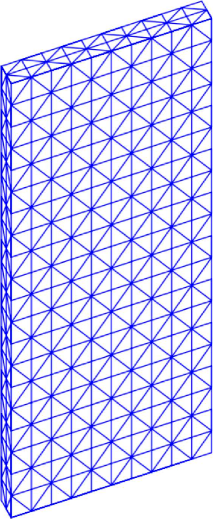
   Figure 1. Slab with its (visible) triangulation, as used here.

2. For the second of our experiments, $\Omega$ has the geometry of the top plate of a classic violin, the Viotti, as per [8]. A computer generated view of this body from above is displayed in Fig. 2. The view, which does not include the $f$-holes, is based on measurements of the actual size images in [8].

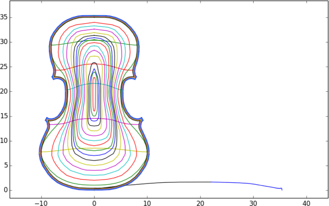
Figure 2. Viotti top plate view (without the $f$ holes) and elevation profile curve.

5.1. Computational complexity

We subdivide the slab of $\text{$10$ cm}\times\text{$1$ cm}\times\text{$20$ cm}$ into $400$ regular blocks of size $\text{$1$ cm}\times\text{$0.5$ cm}\times\text{$1$ cm}$ each, Fig. 1. The resulting triangulation $K$, where the blocks are given the standard subdivision into five tetrahedrons each, contains $693$ vertices, $3,212$ edges, $4,520$ faces and $2,000$ tetrahedrons, and $1,040$ of the faces are boundary faces. The first barycentric subdivision $K^{\prime}$ contains $10,425$ vertices, $61,544$ edges, $99,120$ faces (of which $6,240$ are boundary faces), and $48,000$ tetrahedrons. The two other thinner versions of the slab have triangulations with the same number of elements, merely scaling the depth accordingly. The aspect ratio of their tetrahedrons are half and a quarter of the aspect ratio of those in the first of the triangulations, respectively.

When $\Omega$ is the top plate of the Viotti violin, the triangulation that our work requires is significantly more complex. The top view in Fig. 2, which depicts the outline of this plate, includes the purfling curves, the transversals A, B, C, D, and E, sixteen level sets, and the elevation curve that combines the F and G curves, as per measurements of the images in [8]. The elevation curve serves as a reference for the height of the 16 level sets in the view, with the level of the $j$th set being the elevation at a distance of $j$ cm along it, starting at $0$. This $\Omega$ can be inscribed into a rectangular box of $35.4\,{\rm cm}\times 20.8\,{\rm cm}$. This body is curved, as the 5 transversals to the level sets in the Fig. suggest. The thickness of the plate varies nonuniformly, ranging from a lowest of $0.21$ cm to a largest of $0.36$ cm.

In order to get a reasonable resolution for the type of thickness and curvature that this body has, away from the edge, we subdivide $\Omega$ into blocks of size $\text{$0.5$ cm}\times\text{$0.5d$ cm}\times\text{$0.5$ cm}$, where $d$ is an average thickness of the plate at points where the block is located. We proceed similarly at the edge, but the first dimension of the blocks we consider there is taken to be nonuniform, out of necessity. All in all, it takes 4,608 of these blocks to cover $\Omega$, and the triangulation $K$ that we then derive contains 7,170 vertexes, 35,157 edges, 51,028 faces (of which 10,232 are boundary faces), and 23,040 tetrahedrons. The first barycentric subdivision of this triangulation has 116,395 vertexes, 699,042 edges, 1,135,608 faces, and 552,960 tetrahedrons, with 61,392 of the faces located on the boundary.

In either case, as we traverse the body across the two blocks separating the bounding surface in the thin direction, the barycentric triangulations used contain 444 faces, with 35 intermediate faces separating pair of boundary faces on opposite ends, which when included yield a total 37 faces altogether in going from one side to the other. This provides an adequate resolution for the numerical approximation to accurately capture the true nature of the vibrating wave in these regions, and to propagate in all transversal directions it goes. Refinements of the triangulations that we use would improve the accuracy of the numerical solution, but such would lead to a complexity that is out of the scope of our current computational resources.

As for the boundary conditions that are satisfied by the fine vibration waves approximations, of all the $2\times 6$ subsystems of (29) that the faces in ${{\mathcal{F}}}_{\partial}$ generate, of the 1,040 of them for the slab, exactly eleven have rank one, and of the 10,232 of them for the Viotti plate, exactly one have this property. The differences between these numbers reflect the ${\mathbb{Z}}/2\times{\mathbb{Z}}/2\times{\mathbb{Z}}/2$ symmetry of the triangulation of the slab, as opposed to the nonsymmetric nature of the triangulation of the violin plate, whose thickness varies in a nonuniform manner throughout the body. The astute reader should have noticed that the exterior normal to a boundary face, and its normal as an oriented two simplex, are not necessarily the same.

We find the matrices $I$ and $K$ of the systems (31), (33), by executing python code written for the purpose. The code is structured into four major modules, where just the last one is body specific, an object-oriented conception aimed at making it easy to expand our analysis to bodies with geometries other than those considered here. The processing of the results, and their graphical display, is carried out by some additional python code written for the purpose, the graphical component of it built on top of the PyLab standard library module.

The splitting into interior and boundary faces leads naturally to generating separately the corresponding blocks of these matrices. With a 2.4GHz Intel Core i7 processor, and 8GB 1600 MHz of memory, generating the upper left blocks of the matrices for the slabs takes close to 7h of CPU time each, about 36m for the upper right, and close to 2s for the bottom right. By contrast, for the violin plate, in 10h43m of CPU time we generate 0.59% of the upper left blocks, while in 20h30m we generate 29.35% of the upper right block. The bottom right blocks of the matrices take a time comparable to their alteregos for the slabs. These times are not optimal; they can be improved using the ideas behind the parallelization of the calculations on the basis of the linear ordering of the faces. This, in fact, was the way we managed to complete the generation of the said matrices in the said hardware.

5.2. Elastic constants

We assume that the material that makes our bodies is orthotropic with the elastic constants of spruce. Notice that the arcs of the wedges of either maple or spruce used for a two-piece violin plate subtend a very small angle, and so the transformation from cylindrical to Cartesian coordinates on these wedges is given by a matrix that is very close to the identity, see Remark 3.1 here. Consequently, we take the components of tensors expressed in these two coordinate systems to be the same.

The elastic constants values we use are those in tables 1 & 2 for the Engelmann Spruce. Since these values reflect a failing condition (19), we take the average of the computed values of $\mu_{ij}/e_{i}$ and $\mu_{ji}/e_{j}$ as the value of either one of these quantities in our calculations. Thus, the diagonal blocks of the tensor $W$ of elastic constants (15) in our simulations are

$$W_{3\times 3}=10^{7}\left(\begin{array}[]{ccc}157.198269069862&44.1920517114940&116.065341927474\\ 44.1920517114940&72.0200103705017&75.6887031695923\\ 116.065341927474&75.6887031695923&1095.80735919001\end{array}\right)\,,$$

and

$$D_{3\times 3}=10^{7}\left(\begin{array}[]{ccc}117.480&0&0\\ 0&121.396&0\\ 0&0&9.790\end{array}\right)\,,$$

respectively, the units of the components in Pa. Since we are using an orthonormal frame, we can raise or lower indices in tensors with abandon. We use $\rho=360\;{\rm kg}/{\rm m}^{3}$ for the density parameter. Notice that the eigenvalues of $W_{3\times 3}$ are

$$10^{7}\{156.292790395160,1116.15681336097,52.5760348742398\}\,,$$

so the stored energy function of each of our bodies is coercive.

5.3. Simulations

For each of the bodies with their triangulations as above, we analyze the divergence of the eigenvector solutions, and resonance waves, of the systems (31) and (33), respectively.

5.3.1. The divergence of the coarse and fine normalized eigenvector solutions

The eigenvalues and eigenvectors of the homogeneous systems associated to (31) and (33) are generated using the ARPACK routine eigsh in shift-invert mode, with their corresponding matrix parameters $\rho I$, and $K$, respectively. This computes the solutions $(\lambda,c)$ of the system

$$\rho Ic=\lambda Kc\,.$$

With sigma=-1/(2 pi f)^2, and which=’LM’ passed onto eigsh, we execute the routine for a frequency f any of $80$, $147$, $222$, $304$, and $349$ Hz, respectively. In each case, we produce pairs -((2 \pi f_r)^2, c^{f_r}) of eigenvalue and eigenvector for the matrix $(\rho I)^{-1}K$, where f_r is the eigenvalue of the matrix that is closest to the inputted f, in magnitude, and let

$$U_{f_{r}}=e^{2\pi f_{r}ti}\sum_{W_{f}}c_{f}W_{f}=e^{\omega_{f_{r}}ti}\sum_{W_{f}}c_{f}W_{f}$$

be the corresponding eigenvector wave solution. In the case of the system (31), we let

$$U_{f^{f}_{coarse}}=e^{2\pi f_{coarse}ti}\sum_{W_{f}\in\rm{Div}(K)}c^{f_{coarse}}_{f}W_{f}$$

be the normalized coarse eigenvector solution, while in the case of the system (31), we let

$$U_{f^{f}_{fine}}=e^{2\pi f_{fine}ti}\sum_{W_{f}\in{\rm Div}^{b}(K)}c^{f_{fine}}_{f}W_{f}$$

be the normalized fine eigenvector solution that the said pair produces.

We study the divergence of any normalized eigenvector solution $U=e^{2\pi f_{r}ti}\sum_{W_{f}}c_{f}W_{f}$ by computing the flux

$$\int_{\partial\Omega}U\cdot n\,d\sigma$$

through the boundary of the body at time $t=0$. For the coarse and fine eigenvector solutions, at the frequencies above and for each of the bodies under consideration, the results are as follows:

Body	$f$	$f_{coarse}$333	flux $U_{f^{f}_{coarse}}$	$f_{fine}$333	flux $U_{f^{f}_{fine}}$
Slab 1.0	80	79.89682695	0.0066641031	79.89486045	0.0012710885
	147	146.81041954	-0.0066636678	146.81041954	-0.0012710492
	222	221.71369483	0.0066635620	221.71369483	-0.0012710349
	304	303.60794252	0.0066635192	303.60794252	-0.0012710230
	349	348.54990773	0.0066635053	348.54990774	-0.0012710162
Slab 0.5	80	79.89682695	0.0062420055	79.89682695	0.0032331563
	147	146.81041954	-0.0062419805	146.80677110	0.0032331603
	222	221.71369483	0.0062419720	221.71369483	-0.0032331560
	304	303.60794251	0.0062419656	303.60794251	-0.0032331470
	349	348.54990771	0.0062419620	348.54990772	-0.0032331407
Slab 0.25	80	79.89682695	0.0047848418	79.89682695	-0.0044987163
	147	146.80681943	0.0047851684	146.81041954	-0.0044986653
	222	221.71369483	0.0047852434	221.71369483	-0.0044986514
	304	303.60794250	0.0047852684	303.60794251	-0.0044986436
	349	348.54179550	0.0047852740	348.54990771	-0.0044986401
Viotti plate	80	79.89682695	-0.0026727377	79.93578386	0.0350092360
	147	146.81041953	0.0026739488	146.99894842	0.0350815837
	222	221.71369480	0.0026742324	221.81928975	-0.0033142755
	304	303.60794243	0.0026743267	304.01369231	0.0176140244
	349	348.54990760	0.0026743492	348.54990764	-0.0064094032

Table 3. Initial fluxes for the coarse and fine eigenvector solutions.

5.3.2. Coarse and fine resonance waves

We subject the body to an external sinusoidal pressure wave of the form

$$\vec{F}=\vec{F}_{0}\sin({\bf k}\cdot{\bf x}\mp\omega t)=\vec{F}_{0}\sin({\bf k}\cdot{\bf x})\cos({\omega t})\mp\vec{F}_{0}\cos({\bf k}\cdot{\bf x})\sin({\omega t})$$

that travels in the appropriate direction for it to hit the bottom of the slab, or belly of the Viotti plate, first. If $k=|{\bf k}|$ is the magnitude of the wave vector, we use $v=\omega/k=343$ m/sec, the speed of sound in dry air at $20\mbox{}^{\circ}$C. The source of the wave is placed at a distance of $62$cm from the body, along a line that passes through the height-width plane of the body perpendicularly at the half way point of both, its height and width. This external force induces a force $\vec{F}_{\omega}$ on the body.

The coarse (31) and fine (33) systems are considered with the nonhomogeneous force term arising from the $\vec{F}_{\omega}$ on the body induced by the external wave $\vec{F}$ above, and with trivial initial data. (These are the coarse and fine discrete versions of the initial value problem for (22).) The nonhomogeneous terms in these systems are vectors of the form

$$\vec{C}_{1}\cos{(\omega t)}\mp\vec{C}_{2}\sin{(\omega t)}\,,$$

where $\vec{C}_{1}$ and $\vec{C}_{2}$ are time independent vector fields on the body. If $\omega=2\pi f$ for $f$ any of the frequency values $80$, $147$, $222$, $304$, and $349$ Hz, respectively, we let $\omega_{f_{r}}=2\pi f_{r}$ be the closest eigenvalue to $\omega$ that the matrix $(\rho I)^{-1}K$ has, $\rho I$ and $K$ the matrices of the system in consideration. The resonance wave that this vibration mode produces is given by

(35) $$W_{f_{r}}=\frac{1}{\omega^{2}_{f_{r}}-\omega^{2}}\sum_{W_{f}}\left(c^{W_{f}}_{1}\left(-\cos{(\omega_{f_{r}}t)}+\cos{(\omega t)}\right)\pm c^{W_{f}}_{2}\left(\frac{\omega}{\omega_{f_{r}}}\sin{(\omega_{f_{r}}t)}-\sin{(\omega t)}\right)\right)W_{f}\,,$$

where, for each $j=1,2$, the vector $\vec{c}_{j}=(c_{j}^{W_{f}})$ is the solution to the linear system of equations

$$-((2\pi f)^{2}\rho I+K)\vec{c}_{j}=\vec{C}_{j}\,.$$

The summation is over the basis elements $W_{f}$ of ${\rm Div}(K)$ and ${\rm Div}^{b}(K)$ for the coarse and fine systems, respectively. We generate the vector $\vec{C}_{j}$ as a function of $\vec{F}$, and the geometry of the body, and then solve the system of equations above for $\vec{c}_{j}$ using the scipy.sparse.linalg routine spsolve, with the appropriate parameters.

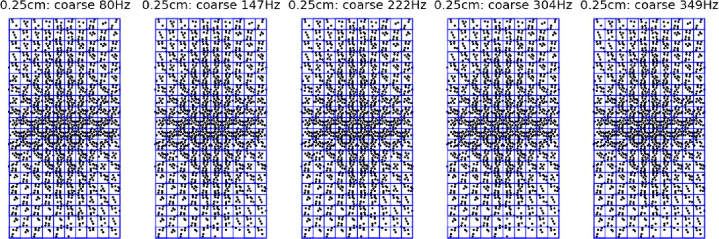
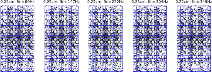
Figure 3. Slab $10\times 0.25\times 20$: Nodal points of the resonance waves at $f$Hz arising from the slab mode of vibration of frequency $f_{r}$ closest to $f$. The notion of nodal point is defined by choosing $c_{\Omega}=0.8$.

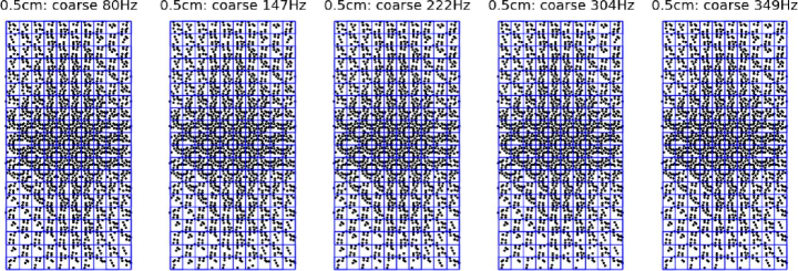
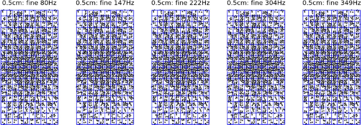
Figure 4. Slab $10\times 0.5\times 20$: Nodal points of the resonance waves at $f$Hz arising from the slab mode of vibration of frequency $f_{r}$ closest to $f$. The notion of nodal point is defined by choosing $c_{\Omega}=0.8$.

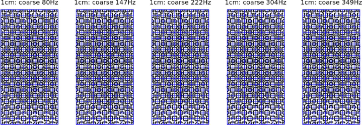
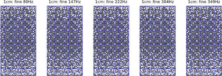
Figure 5. Slab $10\times 1.0\times 20$: Nodal points of the resonance waves at $f$Hz arising from the slab mode of vibration of frequency $f_{r}$ closest to $f$. The notion of nodal point is defined by choosing $c_{\Omega}=0.8$.

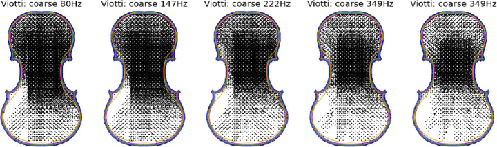
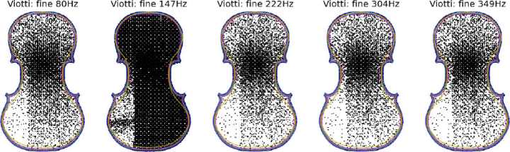
Figure 6. Viotti plate: Nodal points of the resonance waves at $f$Hz arising from the mode of vibration of the plate of frequency $f_{r}$ closest to $f$. The notion of nodal point is defined by choosing $c_{\Omega}=0.04$.

We compute the values of the resonance wave at the barycenter, and vertices, of the boundary faces on the boundary side of the body opposite to the incoming external wave. There are $3,661$ such points for the slabs, and $42,069$ for the Viotti plate. We do these calculations at the equally spaced times $t_{j}=j\frac{2\pi}{10\omega}$, $j=1,\ldots,10$, corresponding to a full cycle of the external wave. For each $t_{j}$, we find the maximum ${\rm max}_{t_{j}}=\max{\{\|W_{f_{r}}(t_{j})\|}\}$ and minimum ${\rm min}_{t_{j}}=\min{\{\|W_{f_{r}}(t_{j})}\|\}$ of the set of norms of the resonance wave at the indicated points, and with $\delta_{t_{j}}=\frac{1}{10}({\rm max}_{t_{j}}-{\rm min}_{t_{j}})$, any of the said points is considered to be nodal at time $t_{j}$ if the norm of the resonance wave solution at the point is no larger than ${\rm min}_{t_{j}}+c_{\Omega}\delta_{t_{j}}$, with $c_{\Omega}=0.8$ for the slabs, and $c_{\Omega}=0.04$ for the Viotti plate, respectively. A point is defined to be nodal if it is nodal at all the $t_{j}$s. All the results for the coarse and fine resonance waves are depicted in Figs. 3-6 below. In each case, we indicate the value of $c_{\Omega}$ that is being used to define a point as nodal.

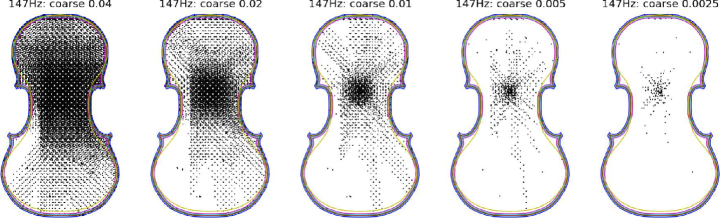
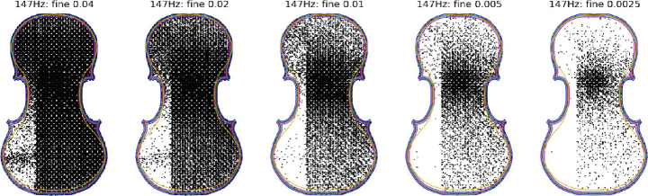
Figure 7. Nodal points of the resonance wave at $f=147$Hz arising from the six mode of vibrations of the plate of frequencies closest to $f$. From left to right, the notion of nodal point is defined by choosing $c_{\Omega}=0.04,0.02,0.01,0.005$ and $0.0025$, respectively.

We study the change in the resulting resonance pattern produced by taking into consideration the six modes with eigenvalues $\omega_{f_{r_{j}}}=2\pi f_{r_{j}}$, $j=1,\ldots,6$, closest to $\omega=2\pi f$, as opposed to the single closest one, as above. The resonance wave is then a sum of six terms as in (35), one per $f_{r_{j}}$s. We exhibit the results for $f=147$Hz in Fig. 7. The five cases depicted correspond to nodal points defined as above for values of $c_{\Omega}=0.04,0.02,0.01,0.005$, $0.0025$, respectively. By comparing the corresponding cases in Figs. 6 and 7, we observe now a better definition of the details of the coarse and fine resonance patterns, though the patterns themselves are not changed significantly (the actual number of nodal points in each of these cases came out to be exactly the same, surely, a coincidence). On the other hand, as the notion of a nodal point becomes stricter by decreasing the value of $c_{\Omega}$, clear details in the resulting patterns emerge, and appear to point quite closely towards the image by holographic interferometry of the mode 2 of a top violin plate in [15, Fig. on p. 177]. Since of the frequencies we consider, the one at which our model for the Viotti plate vibrates the poorest is 147Hz, in spite of the differing conditions between our simulations and the experiments in [15], we take the favorable comparison just made as a validation of our results. The comparison gets better for any of the other values of $f$.

In all of our simulations, for a given geometry and for a given frequency, the fine resonance waves have fewer nodal points than the coarse. For the slabs, the number of nodal points of the resonance waves decreases as the frequency increases, with their values and changes from one to the next smaller and smaller as the thickness decreases. By contrast, these last results are markedly different for the Viotti plate, for which the number of nodal points of the coarse resonance waves decreases as the frequency increases, but the changes are not monotonically decreasing, and the largest of them occurs in going from 147Hz to 222Hz. The pattern is broken altogether for the fine resonance waves, for which, by far, the largest number of nodal points occurs at 147Hz; this number decreases then monotonically for 222Hz and 304Hz to values less than the value it has at 80Hz, and then goes up slightly for the wave associated to 349Hz. The phenomena appears to be more than merely an issue of curvature, perhaps related to wavelength and thickness also, or the combination of (at least) these three elements.

For our simulations for the slabs indicate a limitation to the effect of selective thinning of the plate, a practice among luthiers that is commonly believed to lower or increase frequency modes if carried out in regions of high or low curvature, respectively. The values of the ten quotients ${\rm max}_{t_{j}}/{\rm min}_{t_{j}}$, ordered from smallest to largest, align with thicknesses of 1cm, 0.25cm, and 0.5cm, respectively. At some point, the effect of additional thinning seems to be reversed, and though it would be hard to test this reversal on the already quite thin violin plates, if at all possible, the fact that the Viotti plate has large portions of it that are thinner than the thinnest of the slabs, and the nonmonotonic property of the number of nodal points of its resonance waves, is consistent with this result for the slabs. For the slabs, the largest of the alluded quotients, at a given one of those frequencies used here, is in the order of $10^{3}$; for the Viotti plate, it is in the order of $10^{11}$.

For lack of data on the elastic constants of actual wood used in the making of violin plates, we have not studied possible changes in the results due to the relative humidity of the material. If compared to the original, our model for the Viotti plate should be rather dull, and vibrate poorly, as the data we use is from wood with a high 12% moisture content. (A renowned luthier has told us that the wood he uses to make the plates has moisture content in the range of 2%-5% [7]. This content is likely lowered when the plate is coated with varnish, which adds mass and absorbs some moisture as it dries. Note that the addition of the varnish changes also the flexibility by stiffening the plate across the grain.) We could analyse also temperature increases in the body due to dissipation, or friction, and how they affect the vibration patterns of the plate, but the results of such analyses are out of the scope of the article, as is the study of the resonance pattern under the influence of large exterior pressure forces.

We denote by $W_{f_{coarse}^{f}}$ and $W_{f_{fine}^{f}}$ the normalized coarse and fine resonance wave solutions associated to the pair $(f,f_{r})$ for (31), and (33), respectively. As the waves start with trivial initial condition, we quantify the extent to which our algorithms maintain the divergence free condition throughout time by evaluating their fluxes over the boundary at the time $t_{j}$ where the quotient ${\rm max}_{t_{j}}/{\rm min}_{t_{j}}$ is the largest, and which happens to be $t_{7}$ in all of our simulations. The normalization performed on the resonance waves make these results independent of the magnitude of $\vec{F}_{0}$ in the external wave $\vec{F}$ that induces the resonance. They are listed in Table 4.

Body	$f$	$f_{coarse}$333	flux $W_{f^{f}_{coarse}}$	$f_{fine}$333	flux $W_{f^{f}_{fine}}$
Slab 1.0	80	79.89682695	0.4115594102	79.89486045	0.2154917860
	147	146.81041954	0.4077021407	146.81041954	0.2159199992
	222	221.71369483	0.4009923846	221.71369483	0.2144771805
	304	303.60794252	0.3930235693	303.60794252	0.2119845248
	349	348.54990773	0.3887672035	348.54990774	0.2104879098
Slab 0.5	80	79.89682695	0.4264112637	79.89682695	0.2340175942
	147	146.81041954	0.4225227485	146.80677110	0.2341400584
	222	221.71369483	0.4156736460	221.71369483	0.2322834707
	304	303.60794251	0.4075092711	303.60794251	0.2293410711
	349	348.54990771	0.4031419661	348.54990772	0.2276115430
Slab 0.25	80	79.89682695	0.4312931255	79.89682695	0.2097749790
	147	146.80681943	0.4273781672	146.81041954	0.2096177445
	222	221.71369483	0.4204581119	221.71369483	0.2077423096
	304	303.60794250	0.4122164484	303.60794251	0.2049398128
	349	348.54179550	0.4078257909	348.54990771	0.2033199948
Viotti plate	80	79.89682695	-0.1850124890	79.93578386	-0.0925756811
	147	146.81041953	-0.1091897994	146.99894842	-0.0189475658
	222	221.71369480	-0.0928110618	221.81928975	-0.0426250223
	304	303.60794243	-0.1146617479	304.01369231	-0.0544211220
	349	348.54990760	-0.1354831097	348.54990764	-0.0709637621

Table 4. Fluxes of the normalized coarse and fine resonance waves at time $t_{7}$.

6. Concluding remarks

If we put the computational complexities aside, now we are able to find numerical solutions to the Cauchy problem for the equation of motions of incompressible elastodynamic bodies (1), (2), (3) themselves. We follow the proof of Theorem 2 of [11], and to ignore (1), choose a sufficiently large constant $\lambda$ to modify (2) to

$$\rho\ddot{\eta}(t)(x)={\rm Div}\,W^{{}^{\prime}}(D\eta(t)(x))+J(\eta(t))\nabla q+\lambda J(\eta(t))\nabla_{\eta}J(\eta(t))\,,$$

and modify (3) by adding the condition $J(\eta)=1$ on $\partial\Omega$. Let $({\mathchoice{\rm 1\mskip-4.0mul}{\rm 1\mskip-4.0mul}{\rm 1\mskip-4.5mul}{\rm 1\mskip-5.0mul}},w)$, ${\rm div}\,w=0$ be the Cauchy data, and view the Cauchy problem for the equation above as a nonlinear evolution equation

$$\frac{d}{dt}\left(\begin{array}[]{c}\eta\\ \dot{\eta}\end{array}\right)=G_{\lambda}(\eta,\dot{\eta})$$

with that initial data. If we linearize this equation at a curve $(\eta(t),\dot{\eta}(t))$ satisfying the initial conditions, we obtain a quasilinear system for an unknown $u$ satisfying Cauchy data compatible with $(\eta(0),\dot{\eta}(0))=({\mathchoice{\rm 1\mskip-4.0mul}{\rm 1\mskip-4.0mul}{\rm 1\mskip-4.5mul}{\rm 1\mskip-5.0mul}},w)$. We may apply the algorithm of §4, conveniently changed to account for the modifications in the equations, and obtain a numerical solution $U=U(t)$ to this system. If for sufficiently large $\gamma$ we then consider the equation

$$\gamma\left(\begin{array}[]{c}\zeta\\ \dot{\zeta}\end{array}\right)-G_{\lambda}(\zeta,\dot{\zeta})=-U(t)+\gamma\left(\left(\begin{array}[]{c}\zeta(0)\\ \dot{\zeta}(0)\end{array}\right)+\int_{0}^{t}U(s)ds\right)\,,$$

and solve it for $(\zeta,\dot{\zeta})$ for each fixed $t$, the resulting mapping $(\eta(t),\dot{\eta}(t))\rightarrow(\zeta(t),\dot{\zeta}(t))$ completes the first step of the Newton scheme argument that yields the solution of the Cauchy problem for (1), (2), (3). Iterations of the scheme would produce a sequence $\eta_{n}(t)$ that converges to a solution $\eta$ of the problem on some time interval $[0,T]$. Numerically, we just implemented the first step of this scheme. Should we be able to iterate it at least one more time, we would get a fairly good approximate solution to the free boundary value problem under consideration, with the diffeomorphism numerical solution being reasonably closed to one that preserves volume everywhere.

Any solution $u$ to the linearized equations of motion for (1), (2), (3) about a curve $\eta$ is such that ${\rm div}_{\eta}u=0$, and so if continuous in time, it yields a curve in the Abelian group $H^{2}(M;{\mathbb{R}})$. Our success in overcoming the computational complexities of the problems treated here is in great part the consequence of the algebraic topology encoded into the Whitney forms of the triangulation. It is quite hard to maintain a closed condition as you solve numerically any equation. But if you discretize $u$ in spaces that are natural relative to the cohomology class it represents, the well-posedness of the equation will maintain your numerical solution within reasonable limits of that class throughout time if that condition is made to hold at the start. That remains so when extending the analysis to bodies that have edge and corner singularities. The results of our simulations validate that assertion.

The use of Whitney forms associated to edges is well established [18, 1, 3], though often they are employed to discretize physical quantities that truly represent cohomology classes in degree two, rather than one, and for which the use of the Withney forms associated to faces would be more natural instead. Historically, functions have been approximated by computing their values at sufficiently many points, rather than expanding them as linear combinations of the elements in the partition of unity given by the Whitney forms associated to vertices. Regardless, the use of all of these forms (advocated recently by some [4], though Whitney himself had used them already for several “computational” purposes) is quite natural. If their properties are exploited well, we may capture the essential algebraic structure underlying the problems under consideration, and, with a minimal number of computational elements, derive accurate results for problems with large intrinsic complexities. The geometric content of a triangulation is a powerful tool to use to compute polytope quantities of physical significance [12]; the power of this tool is several times fold larger if we include in the considerations its algebraic content as well.

As indicated earlier, our innovative approach can be extended to the study of vibrational patterns of elastic smooth bodies with corners, under mild assumptions on the stored energy function, generalized Hookian bodies for instance. This is the case of the orthotropic slab that we considered. If the variational principle used to derive the equations of motion is extended to treat cases where part of the boundary is fixed, then we could treat various plates vibrational problems effectively, a cantilever, or several others [16, 2, 5, 6, 14], with the same degree of generality. And since we can obtain the damping vibration modes as easily as the free ones while the motion remains elastic, we could treat the changing temperatures brought about by a dissipation of energy within the body, which in turn brings about changes in the elastic constants, and could eventually lead to breakages if the body is pushed all the way to the nonlinear plastic regime. Our method allows for the use of fundamental principles of physics when solving these problems.

References

- [1] J.S. Asvestas, B. Bielefeld, Y. Deng, J. Glimm, S. Simanca & F. Tangerman, Electromagnetic scattering from large cavities: Iterative methods, Comm. Appl. Anal. 2 (1998), pp. 37-47.
- [2] M. Bennoun, M.S.A. Houari & A. Tounsi, A novel five-variable refined plate theory for vibration analysis of functionally graded sandwich plates, Mech. Adv. Mat. & Struct. 23 (2016), pp. 423-431.
- [3] A. Bossavit, A new rationale for edge-elements, Int. Compumag Soc. Newslett. 1 (1995) pp. 3–6.
- [4] A. Bossavit & F. Rapetti, Whitney forms of higher degree, SIAM J. Numer. Anal. 47 (2009) pp. 2369-2386.
- [5] B. Bouderba, M.S. Ahmed, A. Tounsi & S.R. Mahmoud, On thermal stability of plates with functionally graded coefficient of thermal expansion, Struct. Eng. & Mech. 60 (2016), pp. 313-335.
- [6] A. Bousahla, S. Benyoucef, A. Tounsi & S. Hassan, Thermal stability of functionally graded sandwich plates using a simple shear deformation theory, Struct. Eng. & Mech. 58 (2016), pp. 397-422.
- [7] D. Caron, Private communication. (2018) Taos, NM.
- [8] J. Dilworth, Stradivari ‘Viotti’ violin 1709 poster. The Strad Library.
- [9] J. Dodziuk, Finite-difference approach to the Hodge theory of harmonic forms, Amer. J. Math. 98 (1976), pp. 79-104.
- [10] D.G. Ebin & S.R. Simanca, Small Deformations of Incompressible Bodies with Free Boundary. Comm. in P.D.E., 15 (1990), pp. 1588-1617,
- [11] D.G. Ebin & S.R. Simanca, Deformations of Incompressible Bodies with Free Boundary. Arch. Rational Mech. Anal., 120 (1992), pp. 61-97.
-
[12]
J. Glimm, S.R. Simanca, T. Smith & F. Tangerman, Computational Physics
meets Computational Geometry, preprint (1996), available at
ftp://ftp.ams.sunysb.edu/papers/1996/susb96_19.ps.gz. - [13] D. Green, J. Winandy & D. Kretschmann, Mechanical properties of wood, Wood handbook: wood as an engineering material. Madison, WI: USDA Forest Service, Forest Products Laboratory, 1999. GTR-113: Pages 4.1-4.45
- [14] F. El-Haina, A. Bakora, A.A. Bousahla, A. Tounsi & S.R. Mahmoud, A simple analytical approach for thermal buckling of thick functionally graded sandwich plates, Struct. Eng. & Mech. 63 (2017), pp. 585-595.
- [15] C.M. Hutchins, The Acoustics of Violin Plates, Scientific American, 245 (1981), pp. 171-186.
- [16] A. Mahi, E.A.A. Bedia & A. Tounsi, A new hyperbolic shear deformation theory for bending and free vibration analysis of isotropic, functionally graded, sandwich and laminated composite plates, Appl. Math. Mod. 39 (2015), pp. 2489-2508.
- [17] J.R. Munkres, Elements of algebraic topology. Addison-Wesley Publishing Company, Menlo Park, CA, 1984. ix+454 pp.
- [18] S.M. Rao, D.R. Wilton, & A.W. Glisson, Electromagnetic scattering by surfaces of arbitrary shape, IEEE Trans. Antennas and Propagation, 3 (1982), pp. 409-418.
- [19] M.E. Taylor, Pseudo-Differential Operators, Princeton University Press, 1981.
- [20] H. Whitney, Geometric Integration Theory, Princeton University Press, 1957.