Modeling quantum information dynamics achieved with time-dependent driven fields in the context of universal quantum processing

Abstract

Quantum information is a useful resource to set up information processing. Despite physical components are normally two-level systems, their combination with entangling interactions becomes in a complex dynamics. Studied for piecewise field pulses, this work analyzes the modeling for quantum information operations with fields affordable technologically towards a universal quantum computation model.

1 Introduction

Quantum information takes advantage of quantum physical systems and their properties as superposition and entanglement, where two-level systems are combined and scaled becoming in complex behaviors. Instead of the original states of isolated systems, the use of more advisable non-local basis to set the grammar lets exceed the complexity (polarization or spin). We focus the analysis on magnetic systems for two qubits following the Heisenberg-Ising model with magnetic fields in a fixed direction $h=1,2,3$:

$$H_{h} = \sum_{k=1}^{3}J_{k}{\sigma_{1}}_{k}{\sigma_{2}}_{k}-{B_{1}}_{h}{\sigma_{1}}_{h}-{B_{2}}_{h}{\sigma_{2}}_{h}$$ (1)

here, Bell states recover the binary dynamics [1]. The $SU(4)$ dynamics is split in two subspaces with $SU(2)$ dynamics ($U(1)\rtimes SU(2)^{2}$ as $U_{h}(t)={s_{h}}_{1}\oplus{s_{h}}_{2}$). In terms of Hilbert space: $\mathcal{H}_{h}^{\otimes 2}=\mathcal{H}_{h,1}\oplus\mathcal{H}_{h,2}$, states are split in the subspaces $\left|\psi(t)\right>=\alpha_{1}\left|\psi_{1}(t)\right>+\alpha_{2}\left|\psi_{1}(t)\right>$, $|\alpha_{1}|^{2}+|\alpha_{2}|^{2}=1$ and $\left|\psi_{k}(t)\right>={s_{h}}_{k}\left|\psi_{k}(0)\right>$. Then, $H_{h}=H_{1,h}\oplus H_{2,h}$ [1] with:

$$H_{k,h}\equiv\tilde{H}^{0}_{k,h}+\tilde{H}_{k,h}\rightarrow\tilde{H}^{0}_{k,h}=-s_{0}J_{h}\sigma_{0}^{(h,k)},\quad\tilde{H}_{k,h}=s_{1}{J_{\{h\}}}_{s_{0}}\sigma_{3}^{(h,k)}+s_{2}{B_{h}}_{-s_{0}}\sigma_{q}^{(h,k)}$$ (2)

$\sigma_{i},i=0,...,3$ are the Pauli matrices for a space generated by paired Bell states. $\sigma_{q}^{(h,k)}=-(q-2)\sigma_{1}^{(h,k)}+(q-1)\sigma_{2}^{(h,k)}$, with $s_{0}=(-1)^{h+k+1},s_{1}=s_{0}^{p},s_{2}=(-1)^{p}s_{0}^{p+q}$ and $p=1+\frac{1}{2}(h-1)(h-2),q=2-h{\rm mod}2$ depending on $h,k$, together with the arrangement of pairs of Bell states generating each subspace [1] (not relevant for this development). $J_{h},{J_{\{h\}}}_{s_{0}},{B_{h}}_{-s_{0}}$ are obtained from strengths and fields. The block structure of $\tilde{H}_{k,h}$ for $k=1,2$ is inherited to $U_{h}(t)={s_{h}}_{1}\oplus{s_{h}}_{2}$ through the time ordered integral [2] fulfilling the Schödinger equation. As $\tilde{H}^{0}_{k,h}$ commutes with $\tilde{H}_{k,h}$, by defining ${s_{h}}_{k}\equiv\exp({-\frac{i}{\hbar}}\tilde{H}^{0}_{k,h}){s_{h}}^{0}_{k}$ (revealing the $U(2)=U(1)\times SU(2)$ structure), we get ${s_{h}}^{0}_{k}$ fulfilling the Schödinger equation with $\tilde{H}^{0}_{k,h}$. Then, we will work with $\tilde{H}_{k,h}$ and ${s_{h}}^{0}_{k}$. Analytical solutions for time-independent or stepwise fields exist [3, 4] but they are few feasible because resonant effects.

This work sets a procedure a control procedure with fields as those in resonant cavities, ion traps and laser beams [5, 6, 7, 8]. In the second section, we benchmark linear and quadratic models to solve numerically the time-dependent problem. Third section prescriptions to reduce the evolution into customary processing operations. At the end, we conclude how these results contribute for feasible models of experimental control.

2 Evolution in the time-dependent regime

Baker-Campbell-Hausdorff formula rarely provides closed analytical solutions for time-dependent problems. Alternatively, numerical approaches are necessary. Here, we combine the $SU(2)$ reduction with linear and quadratic approaches to solve the time-dependent problem getting the generic block ${s_{h}}_{j}$ for composite quantum systems. A comparative benchmark is presented at the end. By defining the differential evolution operator $\left|\psi_{k}(t_{0}+\delta t)\right>={s_{h}}^{0}_{k}(t_{0}+\delta t,t_{0})\left|\psi_{k}(t_{0})\right>$ and $J_{h}=\hbar{\mathcal{J}}_{0},-s_{1}{J_{\{h\}}}_{s_{0}}=\hbar{\mathcal{J}}_{s_{0}},-s_{2}{B_{h}}_{-s_{0}}=\hbar{\mathcal{B}}_{-s_{0}}$:

$${s_{h}}^{0}_{k}(t_{0}+\delta t,t_{0}) \approx {\bf 1}_{k}-\frac{i}{\hbar}\tilde{H}_{k,h}(t_{0})\delta t-\frac{i}{2\hbar}\left(\frac{\partial\tilde{H}_{k,h}(t_{0})}{\partial t}+\frac{\tilde{H}^{2}_{k,h}(t_{0})}{i\hbar}\right)\delta t^{2}+...$$ (3)

$$\approx \sigma_{0}^{(h,k)}+iL^{(h,k)}\delta t-\frac{1}{2}Q^{(h,k)}\delta t^{2}+...$$ (4)

with: $L^{(h,k)}={\mathcal{J}}_{s_{0}}\sigma_{3}^{(h,k)}+{\mathcal{B}}_{-s_{0}}(t_{0})\sigma_{q}^{(h,k)}$ and $Q^{(h,k)}=({\mathcal{J}}_{s_{0}}^{2}+{\mathcal{B}}^{2}_{-s_{0}}(t_{0}))\sigma_{0}^{(h,k)}-i{\mathcal{B}}^{\prime}_{-s_{0}}(t_{0})\sigma_{q}^{(h,k)}$. By splitting $[0,t]$ in $n$ intervals $[0,\delta t]\cup...\cup[(n-1)\delta t,n\delta t=t]$ and using (2):

$${s_{h}}_{k} = {s_{h}}_{k}(t,0)\approx{\prod_{i=1,...,n}^{\leftarrow}}{s_{h}}_{k}(i\delta t,(i-1)\delta t)=e^{is_{0}{\mathcal{J}}_{0}t}{\prod_{i=1,...,n}^{\leftarrow}}{s^{0}_{h}}_{k}(i\delta t,(i-1)\delta t)$$ (5)

where $\leftarrow$ means factors stack on the left and $\delta t\approx 0$ is assumed. As in the independent-time case, ${\mathcal{J}}_{0}$ [3] is only responsible from the weak $U(1)$ link between the two $SU(2)$ blocks through $e^{is_{0}{\mathcal{J}}_{0}t}$. (3) is a second order approximation in $\delta t$ for ${s_{h}}_{k}$. We have reduced the dependence ${s_{h}}_{k}$ ($k=1,2$) on the parameters ${\mathcal{J}}_{0},{\mathcal{J}}_{\pm},{\mathcal{B}}_{\pm}(t)$.

3 Construction of universal operations

We fix ${B_{h}}_{\pm}(t)$ in a model applicable for resonant cavities, laser beams, ion traps or superconducting circuits [5, 6, 7, 8]. Despite possible modes ($m=1,2,...$), we will take one single mode $m$. Absorbing physical quantities: $t^{\prime}=\frac{mc}{d}t$ ($d$ an effective wavelength or length in the system) and ${\mathcal{A}}^{\prime}_{\pm}={\mathcal{A}}_{\pm}\frac{d}{mc},{\mathcal{J}}^{\prime}_{\pm}={\mathcal{J}}_{\pm}\frac{d}{mc}$, we assume (dropping the apostrophe):

$${B_{h}}_{\pm}(t) = {\mathcal{A}}_{\pm}\sin(\pi t)$$ (6)

For the numerical approach of ${s_{h}}_{k}$, we develop a benchmark comparing linear and quadratic approximations in (3, 5) (Figure 1a). By running $5\times 10^{4}$ random experiments distributed uniformly on ${\mathcal{J}}_{\pm},{\mathcal{A}}_{\pm}$, we track both the average time of computer processing and the $p$ correct figures reached. The process was repeated for $n$ ranging from $10$ to $10^{4}$, showing at least one figure of improved performance for the quadratic approach in (3), then reducing $n$ from thousands to hundreds. Our implementation (second order and $n=100$) reaches at least five figures of precision. Introducing (6) in (3), we are interested in the reduction of ${s_{h}}_{k}$ into:

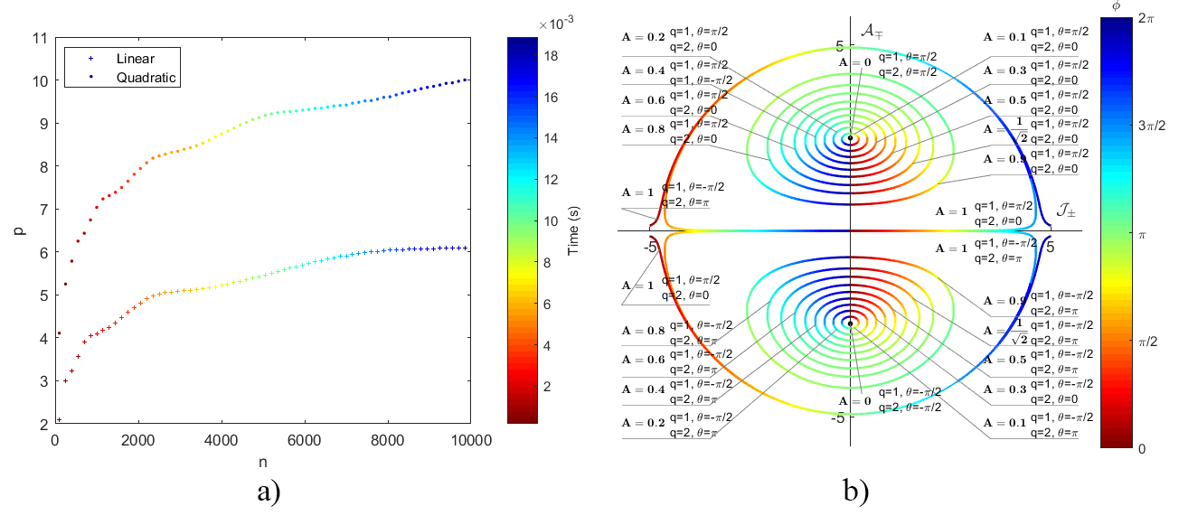
Figure 1: a) Benchmarking for linear and quadratic approximation as function of $n$ (partition), $p$ (digits) and time computer processing (Intel Core i7 2.6GHz); and b) Solutions for ${\mathcal{A}}_{\mp},{\mathcal{J}}_{\pm}$ with $\phi$ in the color chart and $\theta$ as an inset for a set of values for $A$.

$${s_{h}}_{k}=e^{i\varphi}{s_{h}}^{0}_{k}\equiv e^{i\varphi}{\left(\begin{array}[]{cc}Ae^{i\phi}&Be^{i\theta}\\ -Be^{-i\theta}&Ae^{-i\phi}\end{array}\right)}$$ (9)

with $A^{2}+B^{2}=1$. It reduces the dynamics in several traditional quantum processing operations as $C^{a}NOT_{b}$, $NOT$, Hadamard, etc. under the $SU(2)$ reduction scheme [4]. It is affordable imposing restrictions on $A$, and some concrete prescriptions for $\phi,\theta$ and $\varphi$ during $t\in[0,1]$. Figure 1b shows a set of solutions for $A=0,0.1,...,1$ in the region $[-5,5]\times[-5,5]$ of ${\mathcal{A}}_{\pm},{\mathcal{J}}_{\mp}$ plane for $q=1,2$. Insets specify the values of $A,q$ and $\theta$ (unique for each curve) and $\phi$ is reported in the color chart.

4 Conclusions

Solutions obtained for the generic processing operations could be combined under the scheme proposed in [4] for affordable fields as (6). The numerical process developed shows to be efficient to obtain the prescriptions. Then, multi-mode implementations are possible for a common period or otherwise the semi-pulse presented here could be obtained as a superposition of infinite modes as a Fourier series in the set-ups depicted before, letting establish a sequence of semi-pulses corresponding to different gates one followed by another.

References

- [1] Delgado F 2015 Int. J. Quant. Info. 13 1550055
- [2] Grossman M and Katz R 1972 Non-Newtonian calculus (Pigeon Cove, MA: Lee Press)
- [3] Delgado F 2016 J. Phys.: Conf. Series 648 012024
- [4] Delgado F 2017 J. Phys.: Conf. Series 839 012014
- [5] Serikawa T, Shiozawa Y, Ogawa H, Takanashi N, Takeda S, Yoshikawa J and Furusawa A 2018 QIP with a travelling wave of light Proc. SPIE-OPTO 2018 10535
- [6] Britton J, Sawyer B, Keith A, Wang J, Freericks J, Uys H, Biercuk M and Bollinger J 2012 Nature 484 489
- [7] Bohnet J, Sawyer B, Britton J, Wall M, Rey A, Foss-Feig M and Bollinger J 2016 Science 352 6291
- [8] de Sa Neto O and de Oliveira M 2011 Hybrid Qubit gates in circuit QED (quant-ph/1110.1355)