A lower occurrence rate of bright X-ray flares in SN-GRBs than $z<1$ GRBs: evidence of energy partitions?

Abstract

The occurrence rates of bright X-ray flares in $z<1$ gamma-ray bursts (GRBs) with or without observed supernovae (SNe) association were compared. Our Sample I: the $z<1$ long GRBs (LGRBs) with SNe association (SN-GRBs) and with early Swift/X-Ray Telescope (XRT) observations, consists of 18 GRBs, among which only two GRBs have bright X-ray flares. Our Sample II: for comparison, all the $z<1$ LGRBs without observed SNe association and with early Swift/XRT observations, consists of 45 GRBs, among which 16 GRBs present bright X-ray flares. Thus, the study indicates a lower occurrence rate of bright X-ray flares in Sample I (11.1%) than in Sample II (35.6%). In addition, if dim X-ray fluctuations are included as flares, then 16.7% of Sample I and 55.6% of Sample II are found to have flares, again showing the discrepancy between these two samples. We examined the physical origin of these bright X-ray flares and found that most of them are probably related to the central engine reactivity. To understand the discrepancy, we propose that such a lower occurrence rate of flares in the SN-GRB sample may hint at an energy partition among the GRB, SNe, and X-ray flares under a saturated energy budget of massive star explosion.

1 Introduction

Gamma-ray bursts (GRBs) are known as the most luminous electromagnetic explosion in the Universe (see Piran, 2004; Mészáros, 2006; Kumar & Zhang, 2015, for reviews). For example, the total isotropic energy of GRB 160625B can reach $\sim 10^{54}~{}\rm{erg}$ (Wang et al., 2017). Observations show that long-duration, soft-spectrum GRBs (LGRB) are associated with supernovae (SNe) Ib/c (see van Paradijs, 1999; Soderberg, 2006; Woosley & Bloom, 2006; Della Valle, 2007, for reviews), which are generally believed to originate from the collapses of massive stars (Woosley, 1993; MacFadyen & Woosley, 1999; Woosley, Heger, & Weaver, 2002; Heger et al., 2003; Zhang, Woosley, & Heger, 2004; Smartt, 2009; Woosley & Heger, 2012). The direct evidence of the GRBs with SNe association (SN-GRBs) is revealed by Hjorth & Bloom (2012), which classifies the SN-GRBs into five grades as follows. Sample A: spectroscopic SNe; Sample B: a clear light curve bump and some spectroscopic evidence; Sample C: a clear bump consistent with other SN-GRBs put at the spectroscopic redshift; Sample D: a bump, but the inferred SN properties are not fully consistent with other SN-GRBs, or the bump was not well sampled, or there is no spectroscopic redshift for the GRB; Sample E: a bump, either of low significance or inconsistent with other SN-GRBs. Following the spirit of the above classification, Cano et al. (2017b) presented a quite comprehensive database compiled of the observational and physical properties of the GRB prompt emission and SN-GRBs, respectively, which consists of 46 SN-GRBs.

On the other hand, X-ray flares were observed by Swift/X-Ray Telescope (XRT) both in long and short GRBs after the prompt gamma-ray emission (Burrows et al., 2005; Fan & Wei, 2005; Zhang et al., 2006; Nousek et al., 2006; Liang et al., 2006; Falcone et al., 2006; O’Brien et al., 2006). A few flares can occur even up to several days after the GRB trigger (e.g., Chincarini et al., 2007, 2010; Falcone et al., 2007). The physical origins of X-ray flares remain mysterious, which may be related to the late-time activity of the central engine (e.g., Kumar & Panaitescu, 2000; Perna, Armitage, & Zhang, 2006; Dai et al., 2006; Lazzati & Perna, 2007; Falcone et al., 2007; Maxham & Zhang, 2009; Chincarini et al., 2010; Margutti et al., 2010), or to the external shock (e.g., Proga & Zhang, 2006; Giannios, 2006; Curran et al., 2008; Bernardini et al., 2011). The steep decay was observed both in the decay phase of flares and the prompt emission (e.g., Uhm & Zhang, 2016; Jia, Uhm, & Zhang, 2016; Mu et al., 2016b; Lin et al., 2017a, b). Additionally, the high variabilities in the steep decay phase may originate from the activities of the central engine (e.g., Proga et al., 2003; Lei et al., 2007; Liu et al., 2010; Zhang, Zhang, & Castro-Tirado, 2016; Lin et al., 2016). A criterion was introduced to judge the physical origin of X-ray flares, which is based on the relative variability flux and timescale (e.g., Ioka, Kobayashi, & Zhang, 2005; Bernardini et al., 2011; Mu et al., 2016b). The external origin of the flares means that the flares are related to afterglow variability. On the contrary, the internal origin corresponds to the late-time activity of the central engine. Two well-known types of central engines are the hyper-accreting stellar-mass black hole (e.g., Paczynski, 1991; Narayan, Paczynski, & Piran, 1992; MacFadyen & Woosley, 1999; Perna, Armitage, & Zhang, 2006; Luo et al., 2013; Liu, Gu, & Zhang, 2017) and the millisecond magnetar (e.g., Usov, 1992; Duncan & Thompson, 1992; Rees & Mészáros, 2000; Zhang & Mészáros, 2002; Dai et al., 2006; Metzger et al., 2015). For a SN-GRB with an X-ray flare from internal origin, the central engine should account for three explosions, i.e., the supernovae, the prompt gamma-ray emission, and the X-ray flare.

The main purpose of this work is to compare the occurrence rates of X-ray flares in the $z<1$ GRBs with or without observed SNe association, and investigate the physics if significant discrepancy exists between these two rates. The remainder of this paper is organised as follows. Sample selection is presented in Section 2. The main fitting procedure used for X-ray flare data is shown in Section 3. Occurrence rate and physical origin of bright X-ray flares are investigated in Section 4. Discussion and conclusions are summarised in Section 5.

2 Sample selection

A recent review paper, Cano et al. (2017b), presented an up-to-date progress report of the connection between LGRBs and their accompanying SNe. Their sample consists of 46 SN-GRBs, which are classified into five grades, as mentioned in Section 1. In this work, the bright X-ray flares in GRBs with or without observed SNe association were studied. Then, the 46 SN-GRBs in Swift/XRT data were examined to investigate the X-ray afterglow of these sources. The following selection criteria were used to derive a sample of targets.

• (1) The starting point is the sample of Swift/XRT-detected GRBs. We picked only events observed by the Swift/XRT. Thus, 19 GRBs without XRT follow-up observations can be removed (the removed sources can be found by referring to Table 1).

• (2) Since most flares occur in the early time ($t_{\rm{p}}\la 100~{}{\rm{s}}$, Yi et al., 2016), we chose the GRBs with early Swift/XRT follow-up observations (trigger time $\la~{}300~{}\rm{s}$), and therefore eight GRBs were removed.

• (3) In addition, by taking into account the Swift orbital constraint, an adequate X-ray afterglow observation in the early time ($100~{}\rm{s}\sim 1000~{}\rm{s}$) was necessary. Thus, we removed three GRBs with the poor sampling in the early time.

Among the 46 SN-GRBs in Cano et al. (2017b), there are 16 GRBs matching the aforementioned three criteria. Moreover, two recent SN-GRBs, GRB 161219B/SN 2016jca(Ashall et al., 2017; Cano et al., 2017a) and GRB 171205A/SN 2017iuk (Postigo et al., 2017; Prentice et al., 2017), were added to our Sample I. Thus, Sample I consists of 18 GRBs, among which three sources are X-ray Flashes (XRFs) . There are a total of seven XRFs among all the 48 SN-GRBs, which are noted in the first column of Table 1. In addition, the enumerated list pertaining to our sample selection is reported in Table 1, where the related comments are shown in the fourth column.

Table 1: The total 48 SN-GRBs are taken into account in this work, among which the seven XRFs are noted in the first column. The comments in the fourth column: 18 SN-GRBs in Sample I, where the two bright X-ray flares and one dim X-ray fluctuation are denoted as “B” (bright) and “D” (dim) , respectively; 8 GRBs without early Swift/XRT follow-up observations; 3 GRBs with the poor sampling in the early time; 19 GRBs without Swift/XRT observations. The definition of the grades of SN-GRBs are from Hjorth & Bloom (2012) and Cano et al. (2017b), which are shown in the fifth column: Sample $\mathbf{A}$: spectroscopic SNe; Sample $\mathbf{B}$: a clear light curve bump and some spectroscopic evidence; Sample $\mathbf{C}$: a clear bump consistent with other SN-GRBs putting at the spectroscopic redshift; Sample $\mathbf{D}$: a bump, but the inferred SN properties are not fully consistent with other SN-GRBs, or the bump was not well sampled, or there is no spectroscopic redshift for the GRB; Sample $\mathbf{E}$: a bump, either of low significance or inconsistent with other SN-GRBs. The SN-GRB references may refer to Table 1 of Kovacevic et al. (2014) and Table 4 of Cano et al. (2017b).

$\rm{GRB}$	$\rm{SNe}$	z	Comments	Grade
$050416\rm A^{\rm XRF}$	–	0.6528	Sample I	D
$060218^{\rm XRF}$	2006aj	0.03342	Sample I	A
060729	–	0.5428	Sample I	D
060904B	–	0.7029	Sample I(B)	C
070419A	–	0.9705	Sample I	D
080319B	–	0.9371	Sample I	C
081007	2008hw	0.5295	Sample I	B
090618	–	0.5400	Sample I	C
$100316\rm D^{\rm XRF}$	2010bh	0.0592	Sample I	A
100418A	–	0.6239	Sample I	D/E
101219B	2010ma	0.55185	Sample I	A/B
111228A	–	0.7163	Sample I	E
120422A	2012bz	0.2825	Sample I	A
120729A	–	0.8000	Sample I	D/E
130427A	2013cq	0.3399	Sample I	B
130831A	2013fu	0.4790	Sample I(D)	A/B
161219B	2016jca	0.14750	Sample I(B)	A
171205A	2017iuk	0.0386	Sample I	A
$050824^{\rm XRF}$	–	0.8281	no rapid follow-up	E
091127	2009nz	0.49044	no rapid follow-up	B
101225A	–	0.8470	no rapid follow-up	D
111209A	–	0.67702	no rapid follow-up	A/B
111211A	–	0.4780	no rapid follow-up	B/C
130702A	2013dx	0.1450	no rapid follow-up	A
140606B	–	0.3840	no rapid follow-up	A/B
150518A	–	0.2560	no rapid follow-up	C/D
050525A	2005nc	0.6060	poor sampling	B
120714B	2012eb	0.3984	poor sampling	B
150818A	–	0.2820	poor sampling	B
970228	–	0.6950	no XRT	C
980326	–	–	no XRT	D
980425	1998bw	0.00866	no XRT	A
990712	–	0.4330	no XRT	C
991208	–	0.7063	no XRT	E
000911	–	1.0585	no XRT	E
011121	2001ke	0.3620	no XRT	B
020305	–	–	no XRT	E
020405	–	0.6899	no XRT	C
020410	–	–	no XRT	D
$020903^{\rm XRF}$	–	0.2506	no XRT	B
021211	2002lt	1.0040	no XRT	B
030329A	2003dh	0.16867	no XRT	A
$030723^{\rm XRF}$	–	–	no XRT	D
030725	–	–	no XRT	E
$031203^{\rm XRF}$	2003lw	0.10536	no XRT	A
040924	–	0.8580	no XRT	C
041006	–	0.7160	no XRT	C
130215A	2013ez	0.5970	no XRT	B

The XRT light curves of all the 18 SN-GRBs in our Sample I are presented in Figure 1. In this figure, a smooth broken power-law or a single power-law (Beuermann et al., 1999) was used to fit the light curve, and the related fitting parameters are reported in Table 2. We examined the 18 GRBs and searched for bright X-ray flares satisfying the condition “$F_{\rm{p}}>3F$” (e.g., Yi et al., 2016; Mu et al., 2016a), where $F_{\rm{p}}$ and $F$ are the peak flux and the underlying continuum flux at the peak time of the flare, respectively. We found that only two sources, GRBs 060904B and 161219B, have bright X-ray flares, as shown by the mark “B” (bright) in the fourth column of Table 1. Then, the occurrence rate of bright X-ray flares in our Sample I (SN-GRB) is only 11.1%, which seems to be lower than that in the general population.

Table 2: Fitting parameters of the 18 SN-GRBs in our Sample I. From left to right: $\rm{GRB}$, the power-law function parameters ($F_{0}$ and power-law index $\alpha$); the smooth broken power-law function parameters ($F_{1}$, the indices before and after the break time: $\alpha_{1}$ and $\alpha_{2}$, the break time of the flare $t_{\rm{b}}$, the sharpness around peak flux in the flare light curve $w$). The light curve of GRB 060218 is fitted by the sum of two smooth broken power-laws, and therefore the parameters are shown in two lines ($060218^{a}$ and $060218^{b}$). The light curve of GRB 101219B is fitted by the sum of two smooth broken power-laws and one simple power-law, and therefore the parameters are shown in two lines (101219B^a and 101219B^b)

. $\rm{GRB}$ $F_{0}$ $\alpha$ $F_{1}$ $\alpha_{1}$ $\alpha_{2}$ $t_{\rm b}$ $w$ $\rm{red}-\chi^{2}$ $\rm{(erg~{}cm^{-2}~{}s^{-1})}$ $\rm{(erg~{}cm^{-2}~{}s^{-1})}$ (ks) $050416\rm A^{\rm XRF}$ 19.5 $\pm$ 201 5.78 $\pm$ 2.43 ( 1.52 $\pm$ 0.41 )$\times$ $10^{-11}$ 0.37 $\pm$ 0.11 0.9 $\pm$ 0.02 1.55 $\pm$ 0.59 3 0.84 $060218^{\rm XRF,a}$ – – ( 4.73 $\pm$ 0.05 )$\times$ $10^{-9}$ -0.54 $\pm$ 0.01 5.47 $\pm$ 0.04 2.53 $\pm$ 0.02 0.5 – $060218^{\rm XRF,b}$ – – ( 1.52 $\pm$ 0.27 )$\times$ $10^{-12}$ -12.7 $\pm$ 10.08 1.16 $\pm$ 0.06 11.55 $\pm$ 1.12 0.5 1.32 060729 ( 1.10 $\pm$ 0.39 )$\times$ $10^{4}$ 5.39 $\pm$ 0.07 ( 1.42 $\pm$ 0.07 )$\times$ $10^{-11}$ 0.09 $\pm$ 0.03 1.38 $\pm$ 0.02 62.21 $\pm$ 3.01 3 2.17 060904B – – ( 7.79 $\pm$ 5.32 )$\times$ $10^{-12}$ 0.6 1.42 $\pm$ 0.15 5.58 $\pm$ 3.73 3 8.71 070419A 0.27 $\pm$ 0.13 3.64 $\pm$ 0.11 ( 2.40 $\pm$ 2.12 )$\times$ $10^{-13}$ -7.58 $\pm$ 3.45 0.55 $\pm$ 0.15 0.93 $\pm$ 0.99 3 0.78 080319B ( 1.84 $\pm$ 0.05 )$\times$ $10^{-4}$ 1.6 $\pm$ 0.11 – – – – – 2.09 081007 7.46 $\pm$ 1.15 4.83 $\pm$ 0.34 ( 1.67 $\pm$ 0.63 )$\times$ $10^{-12}$ 1.26 $\pm$ 0.07 0.66 $\pm$ 0.03 40.37 $\pm$ 16.61 3 0.97 090618 ( 1.27 $\pm$ 0.41 )$\times$ $10^{7}$ 6.52 $\pm$ 0.07 ( 1.43 $\pm$ 0.09 )$\times$ $10^{-10}$ 0.7 $\pm$ 0.01 1.46 $\pm$ 0.01 6.65 $\pm$ 0.39 3 1.06 $100316\rm D^{\rm XRF}$ – – ( 2.36 $\pm$ 0.04 )$\times$ $10^{-9}$ 0.01 $\pm$ 0.03 2.12 0.98 $\pm$ 0.09 1.5 1.05 100418A ( 5.66 $\pm$ 2.51 )$\times$ $10^{-2}$ 4.01 $\pm$ 0.12 ( 9.21 $\pm$ 1.61 )$\times$ $10^{-13}$ -0.22 $\pm$ 0.1 1.42 $\pm$ 0.09 74.35 $\pm$ 14.85 3 1.54 101219B^a ( 9.59 $\pm$ 5.07 )$\times$ $10^{-6}$ 1.90 $\pm$ 0.09 ( 4.57 $\pm$ 0.28 )$\times$ $10^{-10}$ -0.74 $\pm$ 0.33 5.43 $\pm$ 0.56 0.39 $\pm$ 0.01 3 – 101219B^b – – ( 2.79 $\pm$ 1.08 )$\times$ $10^{-12}$ -1.38 $\pm$ 1.66 0.79 $\pm$ 0.14 6.85 $\pm$ 3.66 0.5 1.05 111228A ( 4.43 $\pm$ 1.68 )$\times$ $10^{3}$ 5.26 $\pm$ 0.08 ( 4.16 $\pm$ 0.77 )$\times$ $10^{-11}$ -0.01 $\pm$ 0.1 1.31 $\pm$ 0.05 7.36 $\pm$ 1.80 1 1.88 120422A ( 4.34 $\pm$ 3.37 )$\times$ $10^{4}$ 6.58 $\pm$ 0.18 ( 1.26 $\pm$ 0.56 )$\times$ $10^{-13}$ 0.29 $\pm$ 0.08 1.18 $\pm$ 0.42 193.4 $\pm$ 133.3 3 1.57 120729A – – ( 1.44 $\pm$ 0.08 )$\times$ $10^{-11}$ 2.6 $\pm$ 0.39 1.03 4.60 $\pm$ 0.75 3 2.01 130427A ( 6.71 $\pm$ 0.12 )$\times$ $10^{-5}$ 1.28 $\pm$ 0.01 ( 7.64 $\pm$ 2.13 )$\times$ $10^{-8}$ 2.39 $\pm$ 0.25 10.1 $\pm$ 1.3 0.31 $\pm$ 0.02 1 1.34 130831A 0.11 $\pm$ 0.30 3.82 $\pm$ 0.5 ( 2.45 $\pm$ 0.59 )$\times$ $10^{-10}$ -0.59 $\pm$ 0.4 1.52 $\pm$ 0.05 1.30 $\pm$ 0.23 3 1.94 161219B ( 1.75 $\pm$ 2.03 )$\times$ $10^{-5}$ 2.42 $\pm$ 0.01 ( 6.37 $\pm$ 3.07 )$\times$ $10^{-10}$ -0.5 $\pm$ 0.73 0.97 $\pm$ 0.1 1.54 $\pm$ 1.66 0.5 8.74 171205A ( 2.24 $\pm$ 0.39 )$\times$ $10^{-4}$ 2.22 $\pm$ 0.03 ( 3.39 $\pm$ 0.31 )$\times$ $10^{-12}$ -1.9 $\pm$ 0.81 1.43 $\pm$ 0.3 49.88 $\pm$ 19.65 0.5 1.69

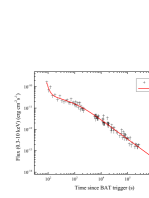
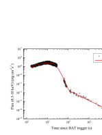
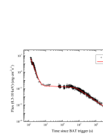
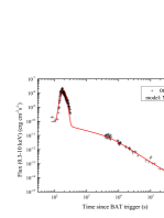
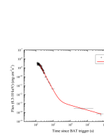
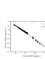
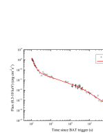
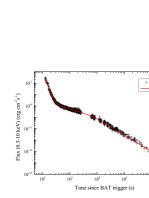
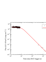
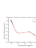
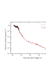
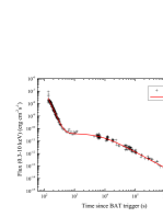
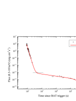
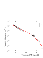
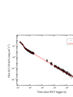
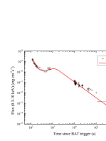
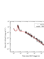
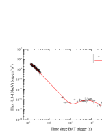
Figure 1: The X-ray light curves of 18 SN-GRBs with early Swift/XRT follow-up observations in our Sample I. The best fitting is shown by the red curves. The smooth broken power-law and single power-law are abbreviated to “bpl” and “pl”, respectively. “N05” (Norris et al., 2005) model means function (2) in the fitting of the bright flares from GRBs 060904B and 161219B.

Since the detection of SNe is limited by the distance, secure SNe identification becomes difficult because the SNe appears fainter at a higher redshift (see, e.g., Woosley & Bloom, 2006). The SN-GRBs in Table 1 exhibit redshift $z<1$ whereas the median redshift of Swift long GRBs is above $2$ (Jakobsson et al., 2006; Salvaterra et al., 2012). Thus, for a comparison, we studied another sample, Sample II, which consists of all the $z<1$ LGRBs between January 2005 and December 2017 that satisfy the aforementioned three criteria, except for the 18 sources in Sample I. In other words, Sample II is composed of the $z<1$ LGRBs with rapid and adequate XRT follow-up observations, and without optically observed SNe association. We should stress that, here the words “without observed SNe association” do not mean “SN-less”. In our opinion, many SN-GRBs may still exist in our Sample II. However, due to observational constraints, accompanying SNe was not observed for those GRBs. The potential influence of such an issue on our results is discussed in the last section. Furthermore, Hjorth & Bloom (2012) showed that SN-less GRBs, such as GRBs 060505 (Fynbo et al., 2006), 060614 (Fynbo et al., 2006; Della Valle et al., 2006; Gal-Yam et al., 2006), and possibly 051109B (Perley et al., 2006) and XRF 040701 (Soderberg et al., 2005), have been observed to deep limits and no accompanying SN is found. Among these sources, only GRBs 051109B and 060614 have XRT rapid follow-up observations, and have adequate observational data in the early time. Since a macronova is likely to be associated with GRB 060614 (Yang et al., 2015), which indicates a merger of two compact objects, 060614 is not included in Sample II. Our Sample II comprises 45 GRBs (44 LGRBs and one XRF), see Table 3 for details. Among all of these 45 GRBs, we found that 16 GRBs have bright X-ray flares, which are denoted as “B” (bright) in the third column of Table 3.

On the other hand, some dim X-ray fluctuations may be regarded as weak X-ray flares. Here we define the dim X-ray fluctuation as the condition “$1.5F<F_{\rm{p}}<3F$” is satisfied. Thus, only one SN-GRB has dim X-ray fluctuation, as denoted by the character “D” (dim) in the fourth column of Table 1. Furthermore, in Sample II, nine GRBs have dim X-ray fluctuations, as reported by “D” (dim) in the third column of Table 3. The number of flares, $N_{\rm flare}$, is also given in the last column of Table 3.

Table 3: Sample II of 45 $z<1$ GRBs. From left to right: 44 LGRBs and one XRF (091018); redshift $z$; bright X-ray flares and dim X-ray fluctuations denoted by “B” (bright) and “D” (dim), respectively; number of flares.

$\rm{GRB}$	$z$	Flare	$N_{\rm flare}$
050219A	0.2115	–	–
050826	0.297	–	–
051016B	0.9364	–	–
051109B	0.08	–	–
060202	0.785	D	1
060512	0.4428	B	1
060814	0.84	D	1
060912A	0.937	–	–
061021	0.3463	–	–
061110A	0.758	–	–
070318	0.84	B	1
070508	0.82	–	–
070521	0.553	–	–
071112C	0.8227	B	1
080430	0.767	–	–
080916A	0.689	–	–
081109	0.9787	–	–
090424	0.544	–	–
090814A	0.696	–	–
$091018^{\rm XRF}$	0.971	–	–
100508A	0.5201	D	1
100621A	0.542	–	–
100816A	0.804	B	1
110715A	0.82	D	1
111225A	0.297	D	1
120722A	0.9586	B	1
120907A	0.97	D	1
130925A	0.347	B	5
131103A	0.599	B	3
140506A	0.889	B	3
140512A	0.725	B	1
140710A	0.558	B	1
141004A	0.57	–	–
150323A	0.593	D	1
150727A	0.313	–	–
150821A	0.755	B	1
151027A	0.81	B	1
160117B	0.86	B	2
160131A	0.97	–	–
160314A	0.726	B	1
160425A	0.555	B	2
160804A	0.736	D	1
161129A	0.645	–	–
170519A	0.818	B	1
170607A	0.557	D	1

3 Fitting procedure

The X-ray flare properties were investigated by fitting the 0.3 $-$ 10 keV(Swift/XRT) light curve with an empirical function proposed by Norris et al. (2005), for $t\geqslant t_{\rm s}$,

$$F_{t}=A\lambda e^{-\frac{\tau_{1}}{t-t_{\rm{s}}}-\frac{t-t_{\rm{s}}}{\tau_{2}}}\ ,$$ (1)

where $\mu=(\tau_{1}/\tau_{2})^{1/2}$ and $\lambda=e^{2\mu}$. The peak time of the flare is $t_{\rm{p}}=\tau_{\rm{p}}+t_{\rm{s}}=(\tau_{1}\tau_{2})^{1/2}+t_{\rm{s}}$. The time of flare onset $t_{\rm{s}}=0$ is adopted in Equation (1). Then, the above equation is simplified as

$$F_{t}=Ae^{2(\tau_{1}/\tau_{2})^{1/2}-\frac{\tau_{1}}{t}-\frac{t}{\tau_{2}}}\ .$$ (2)

Thus, the peak flux of flare is $A=F_{\rm{max}}=F_{\tau_{\rm{p}}}$, and $\tau_{\rm{p}}=(\tau_{1}\tau_{2})^{1/2}$. The flare width is measured between the two $1/e$ intensity points,

$$\omega=\Delta t_{1/e}=\tau_{2}(1+4\mu)^{1/2}.$$ (3)

The fitting results of the X-ray flares are reported in Table 4. In Sample I, each of GRBs 060904B and 161219B has a single bright flare. In Sample II, 26 bright flares exist in 16 GRBs, among which five GRBs have multiple flares and 11 GRBs have a single flare, as shown in the last column of Table 3. In this work, our concerns focus on whether or not, the central engine exhibits reactivity behaviour. As investigated by Bernardini et al. (2011), a sizable fraction of late-time flares (i.e. those with peak time $t_{\rm{p}}\ga 10^{3}~{}\rm{s}$) are compatible with afterglow variability. On the contrary, the early flares are more likely to be related to central engine reactivity. If a GRB has multiple X-ray flares, it is reasonable to judge whether the central engine becomes reactive after the prompt emission by studying the physical origin of the first flare. Thus, for a GRB with multiple flares, only the first flare was fitted. The fitting procedure of GRBs 060904B and 161219B is shown in Figure 2.

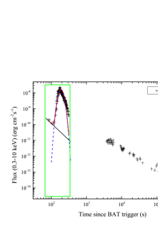
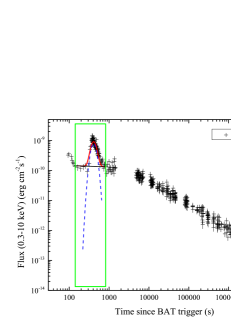
Figure 2: Best fitting for the $0.3-10~{}\rm{keV}$ X-ray afterglow light curve of GRBs 060904B and 161219B (red solid line). Blue dashed line: best fitting for the bright X-ray flare; black solid line: best fitting for the continuous X-ray emission of the underlying continuum. The green box marks the interval of the flare in our fitting.

In addition, to estimate the relative variability flux $\Delta F/F$, where $\Delta F$ and $F$ are the increase of the flux and the underlying continuum flux at the peak time of the flare, respectively, then, the underlying continuum was fitted by using a simple power-law (black solid line, Fig. 2) (e.g., Bernardini et al., 2011; Margutti et al., 2011). The fitting results of the underlying continuum are reported in Table 4. The quantities $t^{\rm{rest}}_{\rm{p}}$ and $\omega^{\rm{rest}}$ are also shown in Table 4, where $t^{\rm{rest}}_{\rm{p}}=t_{\rm{p}}/(1+z)$ and $\omega^{\rm{rest}}=\omega/(1+z)$ are the peak time and width of flares in the rest frame, respectively.

Table 4: Physical parameters from the flares in Sample I and Sample II, and the underlying continuum fitting. From left to right: $\rm{GRB}$, amplitude $\rm{A}$ and the shape parameters $\tau_{1}$, $\tau_{2}$ of the best-fitting of bright X-ray flare from Norris et al. (2005); $t^{\rm{rest}}_{\rm{p}}$ and $\omega^{\rm{rest}}$ are the peak time and width of flares in the rest frame, respectively. $F_{0}$ and $\alpha$ are the parameters of the underlying continuum.

$\rm{GRB}$	$\rm{A}$	$\tau_{1}$	$\tau_{2}$	$t^{\rm{rest}}_{\rm{p}}$	$\omega^{\rm{rest}}$	$F_{0}$	$\alpha$	$\rm{red}-\chi^{2}$
	$\rm{(erg~{}cm^{-2}~{}s^{-1})}$	($10^{3}$ s)	(s)	(s)	(s)	$\rm{(erg~{}cm^{-2}~{}s^{-1})}$
Sample I
060904B	( 1.65 $\pm$ 0.05 )$\times$ $10^{-8}$	4.86 $\pm$ 0.13	7.23 $\pm$ 0.19	110.1 $\pm$ 3.6	43.47 $\pm$ 0.29	( 1.86 $\pm$ 0.62 )$\times$ $10^{-6}$	2.10	8.17
161219B	( 7.76 $\pm$ 0.34 )$\times$ $10^{-10}$	8.27 $\pm$ 0.89	20.38 $\pm$ 2.07	357.7 $\pm$ 30.4	160.4 $\pm$ 1.3	( 1.85 $\pm$ 0.18 )$\times$ $10^{-10}$	0.05 $\pm$ 0.01	2.27
Sample II
060512	( 2.47 $\pm$ 0.38 )$\times$ $10^{-10}$	6.39 $\pm$ 1.85	7.72 $\pm$ 2.21	154.0 $\pm$ 45.2	57.68 $\pm$ 4.06	( 1.25 $\pm$ 0.14 )$\times$ $10^{-6}$	1.80 $\pm$ 0.23	1.56
070318	( 5.90 $\pm$ 0.28 )$\times$ $10^{-10}$	3.64 $\pm$ 0.36	24.19 $\pm$ 2.25	161.2 $\pm$ 20.2	93.01 $\pm$ 0.45	( 1.12 $\pm$ 0.18 )$\times$ $10^{-7}$	1.07 $\pm$ 0.03	1.50
071112C	( 2.76 $\pm$ 0.18 )$\times$ $10^{-10}$	22.78 $\pm$ 4.87	19.34 $\pm$ 3.97	364.2 $\pm$ 98.4	124.8 $\pm$ 2.8	( 5.75 $\pm$ 0.46 )$\times$ $10^{-7}$	1.35 $\pm$ 0.01	1.30
100816A	( 3.30 $\pm$ 0.48 )$\times$ $10^{-10}$	3.31 $\pm$ 1.03	6.58 $\pm$ 1.98	81.8 $\pm$ 31.9	34.75 $\pm$ 2.69	( 1.17 $\pm$ 0.98 )$\times$ $10^{-7}$	1.29 $\pm$ 0.17	1.01
120722A	( 5.64 $\pm$ 0.67 )$\times$ $10^{-11}$	2.86 $\pm$ 1.60	33.00 $\pm$ 15.39	156.9 $\pm$ 111.9	104.2 $\pm$ 1.7	( 2.34 $\pm$ 16 )$\times$ $10^{8}$	8.42 $\pm$ 1.51	0.65
130925A	( 4.14 $\pm$ 0.05 )$\times$ $10^{-9}$	33.86 $\pm$ 0.90	24.38 $\pm$ 0.63	674.4 $\pm$ 16.8	221.7 $\pm$ 0.5	( 5.35 $\pm$ 1.31 )$\times$ $10^{-3}$	2.41 $\pm$ 0.05	1.88
131103A	( 1.54 $\pm$ 0.12 )$\times$ $10^{-9}$	2.35 $\pm$ 0.38	2.83 $\pm$ 0.44	51.0 $\pm$ 9.2	19.09 $\pm$ 2.02	( 1.20 $\pm$ 2.69 )$\times$ $10^{-8}$	0.99 $\pm$ 0.43	1.59
140506A	( 3.80 $\pm$ 0.12 )$\times$ $10^{-8}$	3.04 $\pm$ 0.08	5.19 $\pm$ 0.14	66.5 $\pm$ 2.4	27.17 $\pm$ 0.25	( 1.24 $\pm$ 0.15 )$\times$ $10^{-7}$	0.97 $\pm$ 0.01	2.18
140512A	( 1.50 $\pm$ 0.05 )$\times$ $10^{-8}$	3.10 $\pm$ 0.19	5.14 $\pm$ 0.28	73.2 $\pm$ 5.2	29.69 $\pm$ 0.59	( 7.30 $\pm$ 6.79 )$\times$ $10^{-9}$	0.30 $\pm$ 0.18	0.65
140710A	( 1.22 $\pm$ 0.15 )$\times$ $10^{-10}$	7.62 $\pm$ 1.88	21.04 $\pm$ 4.92	256.9 $\pm$ 68.2	118.6 $\pm$ 2.1	( 6.63 $\pm$ 1.26 )$\times$ $10^{-7}$	1.95 $\pm$ 0.39	1.96
150821A	( 1.56 $\pm$ 0.10 )$\times$ $10^{-10}$	135.4 $\pm$ 41.7	19.03 $\pm$ 5.73	914.4 $\pm$ 345.8	199.4 $\pm$ 10.4	( 1.04 $\pm$ 0.41 )$\times$ $10^{-6}$	1.34 $\pm$ 0.04	0.83
151027A	( 4.50 $\pm$ 0.13 )$\times$ $10^{-8}$	6.21 $\pm$ 0.20	2.53 $\pm$ 0.08	69.2 $\pm$ 2.9	19.71 $\pm$ 0.63	( 1.36 $\pm$ 0.04 )$\times$ $10^{-7}$	0.70 $\pm$ 0.01	1.66
160117B	( 3.24 $\pm$ 0.19 )$\times$ $10^{-9}$	2.53 $\pm$ 0.40	3.09 $\pm$ 0.46	47.5 $\pm$ 9.6	17.84 $\pm$ 1.67	( 8.43 $\pm$ 23 )$\times$ $10^{4}$	7.48 $\pm$ 0.74	3.41
160314A	( 2.75 $\pm$ 0.50 )$\times$ $10^{-11}$	1.25 $\pm$ 0.57	83.55 $\pm$ 25.01	187.5 $\pm$ 87.6	196.6 $\pm$ 0.6	( 3.27 $\pm$ 1.16 )$\times$ $10^{-5}$	2.78 $\pm$ 0.07	0.98
160425A	( 3.38 $\pm$ 0.15 )$\times$ $10^{-8}$	17.60 $\pm$ 0.50	5.36 $\pm$ 0.15	197.5 $\pm$ 6.1	52.29 $\pm$ 0.73	( 5.54 $\pm$ 3.75 )$\times$ $10^{-5}$	2.07 $\pm$ 0.11	7.97
170519A	( 1.14 $\pm$ 0.15 )$\times$ $10^{-8}$	8.16 $\pm$ 2.04	5.70 $\pm$ 1.26	118.7 $\pm$ 35.9	38.72 $\pm$ 3.46	( 1.33 $\pm$ 20 )$\times$ $10^{-5}$	1.73 $\pm$ 2.67	6.80

4 Occurrence rates and physical origin of bright X-ray flares

This work focuses on the occurrence rates of bright X-ray flares in the SN-GRB sample (Sample I) and the general $z<1$ GRBs without observed SNe association (Sample II). As shown in Section 2, for Sample I, among the 18 SN-GRBs (15 LGRBs and three XRFs), only two SN-GRBs have bright X-ray flares, and the occurrence rate is 11.1%. For a comparison, for Sample II, among the 45 GRBs (44 LGRBs and one XRF), 16 sources present bright X-ray flares, and the occurrence rate is 35.6%. Thus, the occurrence rate of X-ray flares in the SN-GRB systems is lower than that in Sample II. In addition, such a discrepancy between these two samples can be examined by the Fisher’s exact test , which shows the one-tailed $P=0.0466\ (<0.05)$. On the other hand, if the dim X-ray fluctuation is included as the weak flare, then 16.7% (3/18) of Sample I and 55.6% (25/45) of Sample II have X-ray flares, again showing the discrepancy between these two samples. Moreover, the Fisher’s exact test shows the one-tailed $P=0.0048\ (\ll 0.05)$. Thus, the discrepancy may indicate that the SN-GRB systems have a lower occurrence rate of X-ray flares than the general $z<1$ GRB systems without observed SNe association. In other words, a lower occurrence rate of X-ray flares may exist in the SN-GRB sample than in the general $z<1$ GRB population.

It should be noted that the physics of X-ray flares may be based on the internal origin or the external one. Ioka, Kobayashi, & Zhang (2005) showed that simple kinematic arguments can give limits on the timescale $\omega$ and amplitude $\Delta F$ of variabilities in GRB afterglows. They proposed that four kinds of afterglow variability are kinematically forbidden under some standard assumptions, and derived the limits for dips (bumps) that deviate below (above) the baseline with a timescale and amplitude (see their Figure 1 for details). These limits are helpful to identify whether or not, the physical origin is afterglow variability or the late-time activity of the central engine. Similar to Ioka, Kobayashi, & Zhang (2005), Bernardini et al. (2011), and Mu et al. (2016a), we plot a figure based on the relative variability flux $\Delta F/F$ and the relative variability timescale $\omega/t_{\rm p}$ to judge the physical origin of the X-ray flares. As shown in Figure 3, most flares are located in the upper left region, which indicates that they are likely to be of internal origin.

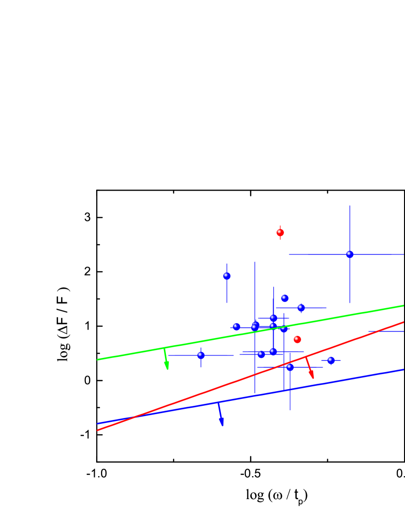
Figure 3: Relationship between the relative variability flux $\Delta F/F$ and the relative variability timescale $\omega/t_{\rm{p}}$ for the X-ray flares in our Sample I and Sample II. The two bright flares from Sample I, which are denoted by the red circles. The 16 bright flares from Sample II are denoted by the blue circles. The four theoretical solid lines are identical with those in Figure 6 of Bernardini et al. (2011), i.e., density fluctuations on axis (blue line) and off-axis (red line), off-axis multiple regions density fluctuations (green line), patchy shell model (black line), see Ioka, Kobayashi, & Zhang (2005) for details.

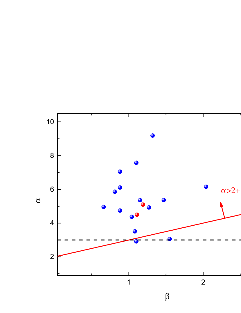
Figure 4: A comparison of the X-ray flares in our two samples with the internal origin $``\alpha>2+\beta"$ (the region above the red solid line) and $``\alpha>3"$ (the region above the black dashed line). The flares from Sample I and Sample II are denoted by the red and blue circles, respectively. The meaning of red and blue circles are the same as in Figure 3.

In another way, by setting the zero time at the GRB trigger time, the flares formed in the external shock process may have a maximum decay slope of $``\alpha=2+\beta"$, where $\beta$ is the spectral index. Consequently, a decay with a slope steeper than $2+\beta$, (i.e., $``\alpha>2+\beta"$), may indicate the internal origin (e.g., Kumar & Panaitescu, 2000; Liang et al., 2006). Such a simple criterion can also be simplified as an even simpler one, $``\alpha>3"$, since $\beta$ is usually around 1. The light curve index $\alpha$ in the decay phase (from $t_{\rm{p}}$ to $t_{\rm{p}}+\tau_{\rm{dec}}$) can be roughly estimated as

$$\alpha=\frac{\log(e)}{\log[(t_{\rm{p}}+\tau_{\rm dec})/t_{\rm{p}}]}\ ,$$ (4)

where $\tau_{\rm{dec}}=\tau_{2}[(1+4\mu)^{1/2}+1]/2$ is the decay time of the flare. The temporal decay index is listed in Table 5. The spectral analyses for the steep decay segments are performed by using a power-law spectral model , The spectral analyses results, i.e., the values of the spectral index in the decay phase $\beta$, are reported in Table 5. It is seen from Figure 4 that, most flares are located above the red solid line and the black dashed line, which implies that most flares are likely to be of internal origin. Such a result is in good agreement with the data shown in Figure 3. We therefore argue that most X-ray flares studied in this work are related to the reactivity of the central engine (Romano et al., 2006; Bernardini et al., 2011; Wu, Hou, & Lei, 2013; Yi et al., 2015).

Table 5: Parameters for the physical origin of Sample I and Sample II. From left to right: $\rm{GRB}$; $\omega/t_{\rm{p}}$ is the relative time-scale, where $\omega$ is the width evaluated between $1/e$ intensity points, and $t_{\rm{p}}$ is the peak time of the flare; $\Delta F/F$ is the relative flux at $t_{\rm{p}}$, and $F$ is calculated from the best fitting of the underlying continuum; $\alpha$ is the temporal decay index; $\beta$ is the average spectral index in the decay phase.

$\rm{GRB}$	$\omega/t_{\rm{p}}$	$\Delta F/F$	$\alpha$	$\beta$
Sample I
060904B	0.39 $\pm$ 0.01	527 $\pm$ 176	5.10	1.19
161219B	0.45 $\pm$ 0.03	5.67 $\pm$ 0.56	4.50	1.11
Sample II
060512	0.37 $\pm$ 0.08	3.38 $\pm$ 0.38	5.37	2.63
070318	0.58 $\pm$ 0.04	2.33 $\pm$ 0.38	3.51	1.08
071112C	0.34 $\pm$ 0.05	3.01 $\pm$ 0.24	5.87	0.81
100816A	0.42 $\pm$ 0.09	1.74 $\pm$ 1.45	4.74	0.88
120722A	0.66 $\pm$ 0.24	210 $\pm$ 143	3.07	1.55
130925A	0.33 $\pm$ 0.01	10.50 $\pm$ 2.57	6.11	0.88
131103A	0.37 $\pm$ 0.04	9.86 $\pm$ 22.13	5.37	1.47
140506A	0.41 $\pm$ 0.01	32.54 $\pm$ 3.91	4.93	1.27
140512A	0.41 $\pm$ 0.02	8.93 $\pm$ 8.25	4.96	0.66
140710A	0.46 $\pm$ 0.08	21.77 $\pm$ 4.14	4.37	1.04
150821A	0.22 $\pm$ 0.05	2.89 $\pm$ 1.12	9.19	1.32
151027A	0.28 $\pm$ 0.01	9.74 $\pm$ 0.31	7.05	0.88
160117B	0.38 $\pm$ 0.04	14.00 $\pm$ 6.08	5.36	1.15
160314A	1.05 $\pm$ 0.28	7.99 $\pm$ 2.84	2.92	1.10
160425A	0.26 $\pm$ 0.01	83.75 $\pm$ 56.66	7.58	1.10
170519A	0.33 $\pm$ 0.05	9.36 $\pm$ 8.81	6.16	2.04

5 Discussion and Conclusions

This work focuses on the different occurrence rates of bright X-ray flares in the $z<1$ GRBs with (Sample I) or without (Sample II) observed SNe association. Our Sample I consists of 18 SN-GRBs, among which only two GRBs have bright X-ray flares. Sample II consists of 45 GRBs, among which 16 GRBs have bright X-ray flares. Our study has shown a lower occurrence rate of bright X-ray flares in the SN-GRB sample (2/18, 11.1%) than in Sample II (16/45, 35.6%). In addition, if the dim X-ray fluctuation is included as a dim flare, then 16.7% (3/18) of the SN-GRB systems and 55.6% (25/45) of Sample II have flares, again showing the discrepancy between these two samples. Thus, the discrepancy may indicate that a lower occurrence rate of X-ray flares may exist in the SN-GRB sample than in the general $z<1$ GRB population.

It is known that there exists a strong selection effect of distance on the luminosity and the total energy of GRBs. In the present work, however, we focus on those close GRBs with $z<1$ , so the selection effect of distance may not be essential. To our knowledge, none of the known selection effects seems to play a role that could account for the apparent deficit of flares in the SN-GRB sample.

As mentioned in the second section, owing to observational constraints, many SN-GRBs may still exist in our Sample II. In addition, we should point out that our work is based on the assumption that there may exist a group of bona fide SN-less LGRBs. Otherwise, our arguments as well as the division of Samples I and II will make less sense. If Sample II does consist of two groups, i.e., SN-GRBs (Sample IIa) and bona fide SN-less GRBs (Sample IIb), we would argue that our main results, i.e., the discrepancy on the occurrence of X-ray flares, can still work. The arguments are as follows. We assume that Samples I, IIa, and IIb have $N_{1}$, $N_{2}$, and $N_{3}$ sources, respectively. If there indeed exists a discrepancy on the occurrence rate of X-ray flares between the SN-GRBs and the bona fide SN-less LGRBs, we assume that the occurrence rate is $f_{1}$ for the former and $f_{2}$ for the latter, with $f_{1}<f_{2}$. Obviously, the real difference in the rates is $(f_{2}-f_{1})$. In such case, according to our analyses based on Samples I and II, the apparent difference will be $[(f_{1}*N_{2}+f_{2}*N_{3})/(N_{2}+N_{3})]-f_{1}=[N_{3}/(N_{2}+N_{3})]\times(f_{2}-f_{1})$, which is even lower than the real one, i.e., $(f_{2}-f_{1})$. In other words, if there exists an apparent discrepancy between Samples I and II, such a discrepancy is likely to be even more significant in the real case (between Sample IIb and Sample I plus IIa). We therefore argue that even though it is not clear how many SN-GRBs exist in our Sample II, the discrepancy suggested in this work may still have potential significance.

In our opinion, the physical understanding of the lower rate of occurrence in the SN-GRB systems may be the following. From the view of the energy source, both the radiation of an SNe and the prompt gamma-ray emission together with the X-ray flare, originate from the total energy of collapse of a massive star, which can be roughly regarded as a saturated energy budget. To produce bright flares, one needs to have in-falling materials near the equatorial direction, which is in the opposite sense of the outgoing materials to power an SN. Thus, bright flares may mean more in-falling materials and therefore less materials are ejected to power the SNe. If this is the case, then it is understandable why the SN-GRB sample has a lower occurrence rate of X-ray flares than Sample II population.

We should point out that, the above argument on the saturated energy budget is only qualitative. In this work, we did not calculate the energy of X-ray flares even though the fitting parameters have been obtained. The reasons for this are as follows. First, a typical ratio of the isotropic energy of a flare to GRB is around 10% (e.g., Chincarini et al., 2010; Yi et al., 2016), which means that the radiation energy of an X-ray flare is generally less than that of the prompt gamma-ray emission. However, the difference in the opening angle and in the energy-release efficiency between the gamma-ray emission and the corresponding flare remains uncertain. It may be less sense to simply add up the two aforementioned parts of the energy budget. In addition, it is difficult to estimate the total energy released through an individual SN, where the neutrino radiation is dominant. Thus, it is beyond the scope of the present work to conduct a detailed energy evaluation. That is why we just focused on whether or not, the central engine has late-time reactivity, and just fitted the first flare but did not investigate, in further detail, the amount of released energy.

On the other hand, the millisecond magnetar may also work as the central engine for GRBs (e.g., Usov, 1992; Duncan & Thompson, 1992; Dai & Lu, 1998; Zhang & Mészáros, 2001; Metzger et al., 2015). It is known that the total amount of available energy of a magnetar is around $2\times 10^{52}~{}\rm{erg}$ (e.g., Thompson, Chang, & Quataert, 2004; Metzger et al., 2011), and perhaps up to $10^{53}~{}\rm{erg}$ (Metzger et al., 2015). In addition, it has been shown that the average kinetic energy of SN-GRBs is around $2\times 10^{52}~{}\rm{erg}$ (Mazzali et al., 2014; Cano et al., 2015), which has implications for the total energy budget. Thus, it is worth undertaking further investigation of the total energy of SN-GRBs to study the type of central engines. A recent interesting work related to this issue, Li et al. (2017), investigated the total energy budget of X-ray plateaus and suggested that a black hole is likely to be operating for most GRBs, and a magnetar central engine is possible for 20% of their analysed GRBs.

References

- Ashall et al. (2017) Ashall C., et al., 2017, arXiv, arXiv:1702.04339
- Bernardini et al. (2011) Bernardini M. G., Margutti R., Chincarini G., Guidorzi C., Mao J., 2011, A&A, 526, A27
- Beuermann et al. (1999) Beuermann K., et al., 1999, A&A, 352, L26
- Burrows et al. (2005) Burrows D. N., et al., 2005, SSRv, 120, 165
- Cano et al. (2015) Cano Z., et al., 2015, MNRAS, 452, 1535
- Cano et al. (2017a) Cano Z., et al., 2017a, A&A, 605, A107
- Cano et al. (2017b) Cano Z., Wang S.-Q., Dai Z.-G., Wu X.-F., 2017b, AdAst, 2017, 8929054
- Chincarini et al. (2010) Chincarini G., et al., 2010, MNRAS, 406, 2113
- Chincarini et al. (2007) Chincarini G., et al., 2007, ApJ, 671, 1903
- Curran et al. (2008) Curran P. A., Starling R. L. C., O’Brien P. T., Godet O., van der Horst A. J., Wijers R. A. M. J., 2008, A&A, 487, 533
- Dai & Lu (1998) Dai Z. G., Lu T., 1998, A&A, 333, L87
- Dai et al. (2006) Dai Z. G., Wang X. Y., Wu X. F., Zhang B., 2006, Sci, 311, 1127
- Della Valle (2007) Della Valle M., 2007, RMxAC, 30, 104
- Della Valle et al. (2006) Della Valle M., et al., 2006, Natur, 444, 1050
- Duncan & Thompson (1992) Duncan R. C., Thompson C., 1992, ApJ, 392, L9
- Evans et al. (2009) Evans P. A., et al., 2009, MNRAS, 397, 1177
- Evans et al. (2007) Evans P. A., et al., 2007, A&A, 469, 379
- Falcone et al. (2006) Falcone A. D., et al., 2006, ApJ, 641, 1010
- Falcone et al. (2007) Falcone A. D., et al., 2007, ApJ, 671, 1921
- Fan & Wei (2005) Fan Y. Z., Wei D. M., 2005, MNRAS, 364, L42
- Fynbo et al. (2006) Fynbo J. P. U., et al., 2006, Natur, 444, 1047
- Gal-Yam et al. (2006) Gal-Yam A., et al., 2006, Natur, 444, 1053
- Greiner et al. (2015) Greiner J., et al., 2015, Natur, 523, 189
- Giannios (2006) Giannios D., 2006, A&A, 455, L5
- Heger et al. (2003) Heger A., Fryer C. L., Woosley S. E., Langer N., Hartmann D. H., 2003, ApJ, 591, 288
- Hjorth & Bloom (2012) Hjorth J., Bloom J. S., 2012, grb..book, 169
- Ioka, Kobayashi, & Zhang (2005) Ioka K., Kobayashi S., Zhang B., 2005, ApJ, 631, 429
- Jakobsson et al. (2006) Jakobsson P., et al., 2006, A&A, 447, 897
- Jia, Uhm, & Zhang (2016) Jia L.-W., Uhm Z. L., Zhang B., 2016, ApJS, 225, 17
- Kovacevic et al. (2014) Kovacevic M., et al., 2014, A&A, 569, A108
- Kumar & Panaitescu (2000) Kumar P., Panaitescu A., 2000, ApJ, 541, L51
- Kumar & Zhang (2015) Kumar P., Zhang B., 2015, PhR, 561, 1
- Lazzati & Perna (2007) Lazzati D., Perna R., 2007, MNRAS, 375, L46
- Lei et al. (2007) Lei W. H., Wang D. X., Gong B. P., Huang C. Y., 2007, A&A, 468, 563
- Li et al. (2017) Li L., Wu X.-F., Lei W.-H., Dai Z.-G., Liang E.-W., Ryde F., 2017, arXiv, arXiv:1712.09390
- Liang et al. (2006) Liang E. W., et al., 2006, ApJ, 646, 351
- Lin et al. (2016) Lin D.-B., Lu Z.-J., Mu H.-J., Liu T., Hou S.-J., Lü J., Gu W.-M., Liang E.-W., 2016, MNRAS, 463, 245
- Lin et al. (2017a) Lin D.-B., Mu H.-J., Liang Y.-F., Liu T., Gu W.-M., Lu R.-J., Wang X.-G., Liang E.-W., 2017a, ApJ, 840, 118
- Lin et al. (2017b) Lin D.-B., Mu H.-J., Lu R.-J., Liu T., Gu W.-M., Liang Y.-F., Wang X.-G., Liang E.-W., 2017b, ApJ, 840, 95
- Liu et al. (2010) Liu T., Liang E.-W., Gu W.-M., Zhao X.-H., Dai Z.-G., Lu J.-F., 2010, A&A, 516, A16
- Liu, Gu, & Zhang (2017) Liu T., Gu W.-M., Zhang B., 2017, NewAR, 79, 1
- Luo et al. (2013) Luo Y., Gu W.-M., Liu T., Lu J.-F., 2013, ApJ, 773, 142
- Mészáros (2006) Mészáros P., 2006, RPPh, 69, 2259
- MacFadyen & Woosley (1999) MacFadyen A. I., Woosley S. E., 1999, ApJ, 524, 262
- Margutti et al. (2010) Margutti R., Guidorzi C., Chincarini G., Bernardini M. G., Genet F., Mao J., Pasotti F., 2010, MNRAS, 406, 2149
- Margutti et al. (2011) Margutti R., et al., 2011, MNRAS, 417, 2144
- Maxham & Zhang (2009) Maxham A., Zhang B., 2009, ApJ, 707, 1623
- Mazzali et al. (2014) Mazzali P. A., McFadyen A. I., Woosley S. E., Pian E., Tanaka M., 2014, MNRAS, 443, 67
- Metzger et al. (2011) Metzger B. D., Giannios D., Thompson T. A., Bucciantini N., Quataert E., 2011, MNRAS, 413, 2031
- Metzger et al. (2015) Metzger B. D., Margalit B., Kasen D., Quataert E., 2015, MNRAS, 454, 3311
- Mu et al. (2016a) Mu H.-J., Gu W.-M., Hou S.-J., Liu T., Lin D.-B., Yi T., Liang E.-W., Lu J.-F., 2016a, ApJ, 832, 161
- Mu et al. (2016b) Mu H.-J., et al., 2016b, ApJ, 831, 111
- Narayan, Paczynski, & Piran (1992) Narayan R., Paczynski B., Piran T., 1992, ApJ, 395, L83
- Norris et al. (2005) Norris J. P., Bonnell J. T., Kazanas D., Scargle J. D., Hakkila J., Giblin T. W., 2005, ApJ, 627, 324
- Nousek et al. (2006) Nousek J. A., et al., 2006, ApJ, 642, 389
- O’Brien et al. (2006) O’Brien P. T., et al., 2006, ApJ, 647, 1213
- Paczynski (1991) Paczynski B., 1991, AcA, 41, 157
- Perley et al. (2006) Perley D. A., Foley R. J., Bloom J. S., Butler N. R., 2006, GCN, 5387, 1
- Perna, Armitage, & Zhang (2006) Perna R., Armitage P. J., Zhang B., 2006, ApJ, 636, L29
- Piran (2004) Piran T., 2004, RvMP, 76, 1143
- Prentice et al. (2017) Prentice S., et al., 2017, ATel1, 11060,
- Proga et al. (2003) Proga D., MacFadyen A. I., Armitage P. J., Begelman M. C., 2003, ApJ, 599, L5
- Proga & Zhang (2006) Proga D., Zhang B., 2006, MNRAS, 370, L61
- Postigo et al. (2017) Postigo A. d. U., Izzo L., Kann D. A., Thoene C. C., Pesev P., Scarpa R., Perez D., 2017, ATel1, 11038
- Rees & Mészáros (2000) Rees M. J., Mészáros P., 2000, ApJ, 545, L73
- Romano et al. (2006) Romano P., et al., 2006, A&A, 450, 59
- Salvaterra et al. (2012) Salvaterra R., et al., 2012, ApJ, 749, 68
- Smartt (2009) Smartt S. J., 2009, ARA&A, 47, 63
- Soderberg (2006) Soderberg A. M., 2006, AIPC, 836, 380
- Soderberg et al. (2005) Soderberg A. M., et al., 2005, ApJ, 627, 877
- Thompson, Chang, & Quataert (2004) Thompson T. A., Chang P., Quataert E., 2004, ApJ, 611, 380
- Uhm & Zhang (2016) Uhm Z. L., Zhang B., 2016, ApJ, 824, L16
- Usov (1992) Usov V. V., 1992, Natur, 357, 472
- van Paradijs (1999) van Paradijs J., 1999, Sci, 286, 693
- Wang et al. (2017) Wang Y.-Z., et al., 2017, ApJ, 836, 81
- Woosley (1993) Woosley S. E., 1993, ApJ, 405, 273
- Woosley & Bloom (2006) Woosley S. E., Bloom J. S., 2006, ARA&A, 44, 507
- Woosley, Heger, & Weaver (2002) Woosley S. E., Heger A., Weaver T. A., 2002, RvMP, 74, 1015
- Woosley & Heger (2012) Woosley S. E., Heger A., 2012, ApJ, 752, 32
- Wu, Hou, & Lei (2013) Wu X.-F., Hou S.-J., Lei W.-H., 2013, ApJ, 767, L36
- Yang et al. (2015) Yang B., et al., 2015, NatCo, 6, 7323
- Yi et al. (2015) Yi S.-X., Wu X.-F., Wang F.-Y., Dai Z.-G., 2015, ApJ, 807, 92
- Yi et al. (2016) Yi S.-X., Xi S.-Q., Yu H., Wang F. Y., Mu H.-J., Lü L.-Z., Liang E.-W., 2016, ApJS, 224, 20
- Zhang & Mészáros (2001) Zhang B., Mészáros P., 2001, ApJ, 552, L35
- Zhang & Mészáros (2002) Zhang B., Mészáros P., 2002, ApJ, 566, 712
- Zhang, Zhang, & Castro-Tirado (2016) Zhang B.-B., Zhang B., Castro-Tirado A. J., 2016, ApJ, 820, L32
- Zhang et al. (2006) Zhang B., Fan Y. Z., Dyks J., Kobayashi S., Mészáros P., Burrows D. N., Nousek J. A., Gehrels N., 2006, ApJ, 642, 354
- Zhang, Woosley, & Heger (2004) Zhang W., Woosley S. E., Heger A., 2004, ApJ, 608, 365