Stretching and Buckling of Small Elastic Fibers in Turbulence

Abstract

Small flexible fibers in a turbulent flow are found to be most of the time as straight as stiff rods. This is due to the cooperative action of flexural rigidity and fluid stretching. However, fibers might bend and buckle when they tumble and experience a strong-enough local compressive shear. Such events are similar to an activation process, where the role of temperature is played by the inverse of Young’s modulus. Numerical simulations show that buckling occurs very intermittently in time. This results from unexpected long-range Lagrangian correlations of the turbulent shear.

Elongated colloidal particles are essentially subject to three dynamical forces: Bending elasticity, thermal fluctuations, and viscous drag with the suspending flow. An important and well-studied case is that of infinitely flexible polymers for which only two effects compete: Coiling promoted by thermal noise, and stretching induced by fluid shear. Relaxation to equilibrium is then fast enough to give grounds for adiabatic macroscopic models, such as elastic dumbbells deGennes1979scaling ; watanabe2010coil , often used to investigate the rheology of polymer suspensions pereira2017active . Much less is known when the thermal fluctuations are negligible but bending elasticity becomes important. This asymptotics is relevant to describe macroscopic particles, such as cellulose fibers in papermaking industry lundell2011fluid , or diatom phytoplankton colonies ardekani2017sedimentation that significantly participate to the CO₂ oceanic pump smetacek1999diatoms . In principle, without molecular diffusion there is no coiling. Furthermore, bending elasticity and flow strain act concomitantly to stretch the fiber, suggesting an unsophisticated stiff rod dynamics. However, most natural or industrial flows are turbulent. They thus display violent and intermittent fluctuations of velocity gradients, susceptible of destabilizing a straight configuration and leading to the buckling of the fiber becker2001instability .

We are interested in elongated, deformable, macroscopic particles passively transported by a turbulent flow. We aim at quantifying two aspects: First, the extent to which their dynamics can be approximated as that of rigid rods and, second, the statistics of buckling. For that purpose, we focus here on the simplest model, the local slender-body theory (see, e.g., lindner2015elastic ), which describes flexible fibers with cross-section $a$ and length $\ell$, as

$$\partial_{t}\bm{X} = \bm{u}(\bm{X},t)+\frac{c}{8\pi\,\rho_{\rm f}\,\nu}\,\mathbb{D}\,\left[\partial_{s}(T\,\partial_{s}\bm{X})-E\,\partial_{s}^{4}\bm{X}\right],$$ (1)

$$|\partial_{s}\bm{X}|^{2}=1,\ \mbox{with }\mathbb{D}=\mathbb{I}+\partial_{s}\bm{X}\,\partial_{s}\bm{X}^{\mathsf{T}},$$

in the asymptotics $c=-[1+2\,\log(a/\ell)]\gg 1$. Here, $\bm{X}(s,t)$ is the spatial position of the point indexed by the arc length coordinate $s\in[-\ell/2,\ell/2]$; $\bm{u}$ is the velocity field of the fluid, $\nu$ its kinematic viscosity and $\rho_{\rm f}$ its mass density; $E$ denotes the fiber’s Young modulus. The tension $T(s,t)$, which satisfies $T|_{\pm\ell/2}=0$, is the Lagrange multiplier associated to the fiber’s inextensibility constraint. Equation (1) is supplemented by the free-end boundary conditions $\partial_{s}^{2}\bm{X}|_{\pm\ell/2}=0$ and $\partial_{s}^{3}\bm{X}|_{\pm\ell/2}=0$.

The considered fibers are much smaller than the smallest active scale of the fluid velocity $\bm{u}$. In turbulence, this means $\ell\ll\eta$, where $\eta=\nu^{3/4}/\varepsilon^{1/4}$ is the Kolmogorov dissipative scale, $\varepsilon\!=\!\nu\langle\|\nabla\bm{u}\|^{2}\rangle$ being the turbulent rate of kinetic energy dissipation. In this limit, the particle motion is to leading order that of a tracer and ${\mathrm{d}\bar{\bm{X}}}/\mathrm{d}t=\bm{u}(\bar{\bm{X}},t)$, where $\bar{\bm{X}}(t)$ denotes its center of gravity. The deformation of the fiber solely depends on the local velocity gradient, so that $\bm{u}(\bm{X},t)\approx\bm{u}(\bar{\bm{X}},t)+\mathbb{A}(t)\,(\bm{X}\!-\!\bar{\bm{X}})$, where $\mathbb{A}_{ij}(t)=\partial_{j}u_{i}(\bar{\bm{X}},t)$. The dynamics is then fully described by two parameters: The fluid flow Reynolds number $\mathrm{Re}$, prescribed very large, and the non-dimensional fiber flexibility

$$\mathcal{F}=\frac{8\pi\,\rho_{\rm f}\,\nu\,\ell^{4}}{c\,E\,\tau_{\eta}},$$ (2)

where $\tau_{\eta}=\sqrt{\nu/\varepsilon}$ is the Kolmogorov dissipative time and quantifies typical values of the turbulent strain rate. The parameter $\mathcal{F}$ can be understood as the ratio between the timescale of the fiber’s elastic stiffness to that of the turbulent velocity gradients. At small $\mathcal{F}$, the fiber is very rigid and always stretched. On the contrary, for large $\mathcal{F}$ it is very flexible and might bend.

In the fully-stretched configuration, the tangent vector is constant along the fiber, i.e. $\partial_{s}\bm{X}=\mathbf{p}(t)$, and follows Jeffery’s equation for straight ellipsoidal rods tornberg2004simulating

$$\frac{\mathrm{d}{\mathbf{p}}}{\mathrm{d}{t}}=\mathbb{A}\,\mathbf{p}-(\mathbf{p}^{\mathsf{T}}\mathbb{A}\,\mathbf{p})\,\mathbf{p}.$$ (3)

This specific solution to (1), which is independent of $s$, is stable when the fiber is sufficiently rigid. However, it becomes unstable when increasing flexibility, or equivalently for larger fluid strain rates. As shown and observed experimentally in two-dimensional velocity fields, such as linear shear becker2001instability ; harasim2013direct ; liu2018tumbling or extensional flows young2007stretch ; wandersman2010buckled ; kantsler2012fluctuations , this instability is responsible for a buckling of the fiber. This occurs when the elongated fiber tumbles schroeder2005characteristic ; plan2016tumbling and experiences a strong-enough compression along its direction. This compression is measured by projecting the velocity gradient along the rod directions, i.e. by the shear rate $\dot{\gamma}=\mathbf{p}^{\mathsf{T}}\mathbb{A}\,\mathbf{p}$. In turbulence, buckling thus occurs when the instantaneous value of $\dot{\gamma}$ becomes large with a negative value (compression).

To substantiate this picture we have performed direct numerical simulations. The flow is obtained by integrating the incompressible Navier–Stokes equations using the LaTu spectral solver with $4096^{3}$ collocation points and with a force maintaining constant the kinetic energy content of the two first Fourier shells (see, e.g., homann2007impact ). Once a statistically stationary state is reached with a Taylor micro-scale Reynolds number $\mathrm{Re}_{\lambda}\approx 730$, the flow is seeded with several thousands of tracers, along which the full velocity gradient tensor is stored with a period $\approx\tau_{\eta}/4$. The local slender-body equation for fibers (1) is then integrated a posteriori along these tracer trajectories. We use the semi-implicit, finite-difference scheme introduced in tornberg2004simulating , with the inextensibility constraint enforced by a penalization procedure. $N=201$ grid points are used along the fibers arc-length coordinate, with a time step $5\times 10^{-4}\,\tau_{\eta}$. We use linear interpolation in time to access the velocity gradient at a higher frequency than the output from the fluid simulation.

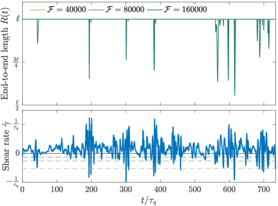
Figure 1: Top panel: Time evolution of the end-to-end length $R(t)$ for a specific turbulent tracer trajectory and three different values of the non-dimensional flexibility $\mathcal{F}$, as labeled. Bottom panel: Evolution of the instantaneous shear rate $\dot{\gamma}$ along the same trajectory. The solid line corresponds to $\dot{\gamma}=0$ and the dashed lines to $\tau_{\eta}\,\dot{\gamma}=-0.13$, $-0.26$, and $-0.52$. Note that time is rescaled by the Kolmogorov timescale $\tau_{\eta}$. In these units, the large-eddy turnover time is $\tau_{L}\approx 190\,\tau_{\eta}$.

Numerics confirm that fibers much smaller than the Kolmogorov scale are almost always stretched. This can be measured from the end-to-end length $R(t)=|\bm{X}(\ell/2,t)-\bm{X}(-\ell/2,t)|$. When $R=\ell$, the fiber is straight. Buckling occurs when $R<\ell$. The upper panel of Fig. 1 shows the time evolution of the end-to-end length along a single trajectory for various non-dimensional flexibilities $\mathcal{F}$. Clearly, bending is sparse and intermittent. Buckling events are separated by long periods during which $R\equiv\ell$, up to numerical precision. For instance, one observes $|1-R(t)/\ell|<10^{-13}$ in the time interval $100<t/\tau_{\eta}<180$. In the lower panel of Fig. 1, we have shown the time evolution of the shear rate $\dot{\gamma}$ along the same Lagrangian trajectory. As expected, buckling events are associated to strong negative fluctuations of $\dot{\gamma}$. Note that, because $\mathbf{p}$ is preferentially aligned with the fluid stretching ni2014alignment , the shear rate has a positive mean $\langle\dot{\gamma}\rangle\approx 0.11/\tau_{\eta}$. Its standard deviation is $\approx 0.2/\tau_{\eta}$.

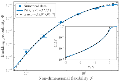
Figure 2: Probability of buckling $\Phi$ as a function of $\mathcal{F}$. The squares come from numerical simulations and were calculated as the fraction of time during which $R(t)/\ell<0.999$. Error bars are obtained from the standard deviation of the duration of individual events. The bold line is the probability that the shear rate $\dot{\gamma}$ is less than $-\mathcal{F}^{\star}/(\tau_{\eta}\,\mathcal{F})$ with $\mathcal{F}^{\star}=2.1\times 10^{4}$. The corresponding cumulative distribution function (CDF) is shown in the inset, together with a fit (dashed line) of the form $\propto\exp[-A\,(\tau_{\eta}\,|\dot{\gamma}|)^{1/2}]$, where $A=1.69$. The same approximation is used in the main panel to fit $\Phi$ (dashed line).

To get more quantitative insights, we define buckling events as times when $R(t)/\ell$ is below a prescribed threshold (we have used $0.999$). Figure 2 shows the probability of buckling as a function of the flexibility $\mathcal{F}$. This quantity, denoted $\Phi$, is defined as the fraction of time spent by the end-to-end length below this threshold. One finds that, conversely to simple steady shear flows (see, e.g., lindner2015elastic ), in turbulence there is no critical value of the flexibility above which buckling occurs. Fibers bending is similar to an activated process with $\Phi\propto\exp(-C/\mathcal{F}^{\alpha})$ and where the flexibility $\mathcal{F}$ plays a role resembling that of temperature in chemical reactions. Indeed, the fiber will buckle when its instantaneous flexibility $\mathcal{F}_{\rm loc}(t)=\tau_{\eta}\,|\dot{\gamma}(t)|\,\mathcal{F}$ is larger than a critical value $\mathcal{F}^{\star}$, with $\dot{\gamma}(t)<0$. This leads to

$$\Phi=\mathrm{Pr}\,\left(\tau_{\eta}\,\dot{\gamma}<-\mathcal{F}^{\star}/\mathcal{F}\right).$$ (4)

As can be seen in Fig. 2, the cumulative probability of the shear rate can indeed be used to reproduce the numerical measurements of $\Phi$ by choosing $\mathcal{F}^{\star}=2.1\times 10^{4}$. This value, which just corresponds to a fit, is much larger than those observed in time-independent shear flows liu2018tumbling where buckling occurs for $\mathcal{F}\gtrsim 300$. A first reason comes from using the Kolmogorov dissipative timescale when defining $\mathcal{F}$. This is a natural but arbitrary choice in turbulence. However $\tau_{\eta}$ is significantly smaller than typical values of $\dot{\gamma}^{-1}$, so that effective flexibilities could be smaller than $\mathcal{F}$. This is similar to choosing $\tau_{\eta}$ rather than the Lyapunov exponent to define the Weissenberg number for the coil-stretch transition of dumbbells in turbulent flow boffetta2003two . Another explanation for a large $\mathcal{F}^{\star}$ could be the intricate relation in turbulence between the amplitude of velocity gradients and their dynamical timescales, which implies in principle that the stronger is $\dot{\gamma}$, the shorter is the lifetime of the associated velocity gradient.

Fibers with a small flexibility buckle only when the instantaneous shear rate is sufficiently violent. Moreover it is known that at large Reynolds numbers kailasnath1992probability , the probability distribution of velocity gradients has stretched-exponential tails with exponent $\approx 1/2$. This behavior is also present in the cumulative probability of $\dot{\gamma}$, as seen in the inset of Fig. 2. This leads to predict that

$$\Phi\propto\mathrm{e}^{-A\,\left({\mathcal{F}^{\star}}/{\mathcal{F}}\right)^{1/2}}\mbox{ for }\mathcal{F}\ll\mathcal{F}^{\star}.$$ (5)

This asymptotic behavior is shown as a dashed line in the main panel of Fig. 2. It gives a rather good fit of the data, up to $\mathcal{F}\approx 1.6\times 10^{5}$. At larger values, this activation-like asymptotics and relation to the tail of the distribution is no more valid. At very small values (or equivalently large negative $\dot{\gamma}$’s), one observes tiny deviations from the stretched exponential, certainly resulting from numerical errors over-predicting extreme gradients buaria2017resolution .

The relevance to buckling of an instantaneous flexibility larger than $\mathcal{F}^{\star}$ can be seen in Fig. 1. The dashed lines on the bottom panel are the critical values $\tau_{\eta}\,\dot{\gamma}=-\mathcal{F}^{\star}/\mathcal{F}$ associated to the three flexibilities of the top panel. We indeed observe that buckling occurs when the instantaneous shear rate underpasses these values. In some cases (e.g. for times between $400$ and $500\,\tau_{\eta}$), it seems that the fiber is straight, even if $\dot{\gamma}$ is below the threshold. Still, buckling occurs but with an amplitude so small that it cannot be detected from the top panel. This threshold therefore provides information on the occurence of buckling, but not on the strength of the associated bending.

Another qualitative assessment that can be drawn from Fig. 1 is that large excursions of $\dot{\gamma}$ are not isolated events but form clumps. This is a manifestation of the Lagrangian intermittency of velocity gradients. Tracers might indeed be trapped for long times in excited regions of the flow, leading to fluctuations correlated over much longer times than $\tau_{\eta}$. This can be quantified from the autocorrelation $\rho(t)$ of the negative part $\dot{\gamma}^{-}=\max(-\dot{\gamma},0)$ of the shear rate, which is represented in the inset of Fig. 3. The corresponding integral correlation time is $\int\rho(t)\,\mathrm{d}t\approx 2.8\,\tau_{\eta}$. This can be explained by the abrupt decrease of the autocorrelation at times of the order of the Kolmogorov timescale. This behavior is essentially a kinematic effect due to fast rotations. Remember that $\dot{\gamma}$ is obtained by projecting the velocity shear on the direction $\mathbf{p}$ of a rigid rod. This direction rotates with an angular speed given by the vorticity $\omega=|\nabla\times\bm{u}|$, so that $\dot{\gamma}$ can alternate from expansion to compression, on timescales of the order of $\omega^{-1}\sim\tau_{\eta}$. Surprisingly, at longer times $t\gtrsim 4\,\tau_{\eta}$, the autocorrelation of $\dot{\gamma}^{-}$ changes regime and decreases much slower than an exponential. This contradicts the classical phenomenological vision that velocity gradients are purely a small-scale quantity with correlations spanning only the dissipative scales. For more than a decade in $t$ within the inertial range, we indeed find a power-law behavior $\rho(t)\propto t^{-\beta}$, with $\beta\approx 0.7\pm 0.1$. To our knowledge, this is the first time such a long-range behavior is observed for turbulent Lagrangian correlations.

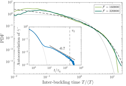
Figure 3: Probability density functions (solid lines) of the time $T$ between successive buckling events, normalized to its average $\langle T\rangle\approx 52\,\tau_{\eta}$ for $\mathcal{F}=1.6\times 10^{5}$, and $\langle T\rangle\approx 36\,\tau_{\eta}$ for $\mathcal{F}=3.2\times 10^{5}$. The dotted line represents the exponential distribution. The dashed line is a Weibull distribution (6) with shape parameter $\beta=0.7$ and scale parameter $\lambda=1$. Inset: Autocorrelation $\rho(t)=\mathrm{cov}\left(\dot{\gamma}^{-}(t),\dot{\gamma}^{-}(0)\right)/\mathrm{Var}(\dot{\gamma}^{-})$ of the negative part of the shear rate. The dotted line stands for $\exp(-t/\tau_{\eta})$; The vertical dashed line indicates the large-eddy turnover time $t=\tau_{L}$; The solid line shows a slope $-0.7$.

These intricate correlations have important consequences on the incidence of buckling. Memory effects are present, as the fiber is likely to bend several times when in a clump of violent, high-frequency fluctuations of $\dot{\gamma}$. Consequently, the probability distribution $p(T)$ of the time $T$ between successive buckling events is not an exponential. This is clear from the main panel of Fig. 3, where this distribution is shown for $\mathcal{F}=1.6\times 10^{5}$ and $3.2\times 10^{5}$. One observes clear deviations from the exponential distribution (dotted line). They relate to the two regimes discussed above for the time correlations of $\dot{\gamma}^{-}$. First, the distribution of inter-buckling times is maximal for $T$ of the order of $\tau_{\eta}$. This corresponds to rapid oscillations of the sign of $\dot{\gamma}$. The fiber experiences several tumblings in an almost-constant velocity gradient and is alternatively compressed and pulled out by the flow due to fast rotations. This leads to a rapid succession of bucklings and stretchings. Second, strong deviations to the exponential distribution also occur for inter-buckling times $T$ in the inertial range. As seen in Fig. 3, the distribution of inter-buckling times in the intermediate range $0.5\lesssim T/\langle T\rangle\lesssim 5$ is well approximated by a Weibull distribution with shape $\beta$ and scale parameter $\lambda$:

$$p(T)\approx\frac{\beta\,T^{\beta-1}}{\lambda^{\beta}}\,\mathrm{e}^{-\left({T}/{\lambda}\right)^{\beta}}.$$ (6)

This decade exactly matches the time lags for which $\dot{\gamma}$ displays long-range correlations, that is $\rho(t)\sim t^{-\beta}$. The return statistics of processes with power-law correlations is indeed expected to be well approximated by a Weibull distribution eichner2007statistics . Longer times correspond to $t\gtrsim\tau_{L}$, for which $p(T)$ is expected to ultimately approach an exponential tail.

Figure 4: Contour levels of the joint distribution of the end-to-end length $R$ and of the mean curvature $\bar{\kappa}$ for $\mathcal{F}=1.6\times 10^{5}$. The vertical dashed line shows the threshold $R/\ell=0.999$. Two excursions of the same trajectory as Fig. 1 are shown for $43<t/\tau_{\eta}<77$ (red) and $680<t/\tau_{\eta}<730$ (orange). Also, two instantaneous configurations of the fiber are represented for $t=43\,\tau_{\eta}$ (top left) and $t=45\,\tau_{\eta}$ (bottom right).

To characterize further buckling events and in particular their geometry, we show in Fig. 4 the joint probability density of the end-to-end length $R$ and of the fiber’s mean curvature $\bar{\kappa}=(1/\ell)\int|\partial_{s}^{2}\bm{X}|\,\mathrm{d}s$. The distribution is supported in a thin strip aligned with $\bar{\kappa}\propto(1-R/\ell)^{1/2}$. Bucklings correspond to loops in this plane. Trajectories typically start such excursions with a larger curvature (upper part of the strip) than the one they have when relaxing back to a straight configuration (lower part). The red curve corresponds to the first buckling event of the trajectory shown in Fig. 1. The curvature increases concomitantly to a decrease of the end-to-end length. Right before reaching a maximal bending, the fiber displays several coils (top-left inset). This configuration depends on the most unstable mode excited with the current value of the instantaneous flexibility $\mathcal{F}_{\rm loc}$. It is indeed known that buckling fibers in steady shear flows can experience several bifurcations, depending on their elasticity becker2001instability . Once the fiber has again aligned with $\dot{\gamma}>0$, that is a couple of $\tau_{\eta}$’s later, these coils unfold (bottom-right inset), the curvature decreases, and the fiber relaxes back to a fully stretched configuration. This specific event has been chosen for its simplicity and representativity. In the case of high-frequency buckling discussed earlier, such as shown in orange, the fiber experiences multiple buckling. The time is now $t\approx 700\,\tau_{\eta}$, for which we observe in Fig. 1, several oscillations of $\dot{\gamma}$. The fiber is alternatively compressed and stretched, leading here to six successive bendings, separated by only a few $\tau_{\eta}$’s.

To conclude, recall that we have focused on passively transported fibers. In several applications, they actually have an important feedback on the flow and might even reduce turbulent drag. We found here that the dynamics of flexible fibers strongly depends on the shear strength: In calm regions, they just behave as stiff rods. In violent, intermittent regions, they can buckle, providing an effective transfer of kinetic energy toward bending elasticity. Such nonuniform, shear-dependent effects likely lead to intricate flow modifications, where the presence of small fibers affects not only the amplitude of turbulent fluctuations, but also their very nature. Such complex non-Newtonian effects undoubtedly lead to novel mechanisms of turbulence modulation.

This work has been supported by EDF R&D (projects PTHL of MFEE and VERONA of LNHE) and by the French government, through the Investments for the Future project UCA^JEDI ANR-15-IDEX-01 managed by the Agence Nationale de la Recherche.

References

- (1) P.-G. De Gennes, Scaling concepts in polymer physics (Cornell University Press,Ithaca, NY, 1979).
- (2) T. Watanabe and T. Gotoh, Phys. Rev. E 81, 066301 (2010).
- (3) A.S. Pereira, G. Mompean, L. Thais, E.J. Soares, and R.L. Thompson, Phys. Rev. Fluids 2, 084605 (2017).
- (4) F. Lundell, L.D. Söderberg, and P.H. Alfredsson, Annu. Rev. Fluid Mech. 43, 195 (2011).
- (5) M.N. Ardekani, G. Sardina, L. Brandt, L. Karp-Boss, R. Bearon, and E. Variano, J. Fluid Mech. 831, 655 (2017).
- (6) V. Smetacek, Protist 150, 25 (1999).
- (7) L.E. Becker and M.J. Shelley, Phys. Rev. Lett. 87, 198301 (2001)
- (8) A. Lindner and M.J. Shelley, in Fluid-Structure Interactions in Low-Reynolds-Number Flows (Royal Society of Chemistry, 2015) pp. 168–192.
- (9) A.K. Tornberg and M.J. Shelley, J. Comput. Phys. textbf196, 8 (2004)
- (10) M. Harasim, B. Wunderlich, O. Peleg, M. Kröger, and A.R. Bausch, Phys. Rev. Lett. 110, 108302 (2013).
- (11) Y. Liu, B. Chakrabarti, D. Saintillan, A. Lindner, and O. du Roure, “Tumbling, buckling, snaking: Morphological transitions of elastic filaments in shear flow”, Preprint arXiv:1803.10979
- (12) Y.-N. Young and M.J. Shelley, Phys. Rev. Lett. 99, 058303 (2007).
- (13) E. Wandersman, N. Quennouz, M. Fermigier, A. Lindner, and O. Du Roure, Soft Matter 6, 5715 (2010).
- (14) V. Kantsler and R.E. Goldstein, Phys. Rev. Lett. 108, 038103 (2012).
- (15) C.M. Schroeder, R.E. Teixeira, E.S. Shaqfeh, and S. Chu, Phys. Rev. Lett. 95, 018301 (2005).
- (16) E. Plan and D. Vincenzi, Proc. R. Soc. A 472, 20160226 (2016).
- (17) H. Homann, J. Dreher, and R. Grauer, Comput. Phys. Comm. 177, 560 (2007).
- (18) R. Ni, N.T. Ouellette, and G.A. Voth, J. Fluid Mech. 743 (2014).
- (19) G. Boffetta, A. Celani, and S. Musacchio, Phys. Rev. Lett. 91, 034501 (2003).
- (20) P. Kailasnath, K. Sreenivasan, and G. Stolovitzky, Phys. Rev. Lett. 68, 2766 (1992).
- (21) D. Buaria, A. Pumir, E. Bodenschatz, and P.K. Yeung, “Resolution effects and the structure of extreme velocity gradients in high Reynolds number turbulence”, in APS Meeting Abstracts (2017).
- (22) J.F Eichner, J.W. Kantelhardt, A. Bunde, and S. Havlin, Phys. Rev. E 75, 011128 (2007).