Nonreciprocal charge transport in two-dimensional noncentrosymmetric superconductors

Abstract

Nonreciprocal charge transport phenomena are studied theoretically for two-dimensional noncentrosymmetric superconductors under an external magnetic field $B$. Rashba superconductors, surface superconductivity on the surface of three-dimensional topological insulators (TIs), and transition metal dichalcogenides (TMD) such as MoS₂ are representative systems, and the current-voltage $I$-$V$ characteristics, i.e., $V=V(I)$, for each of them is analyzed. $V(I)$ can be expanded with respect to the current $I$ as $V(I)=\sum_{j=1,\infty}a_{j}(B,T)I^{j}$, and the $(B,T)$-dependence of $a_{j}$ depends on the mechanism of the charge transport. Note that the magnetochiral anisotropy in the normal state is expressed by $a_{1}(B,T)=R_{0}$ and $a_{2}(B,T)=R_{0}\gamma B$ with the constant $\gamma$. Our analysis is based on the time-dependent Ginzburg-Landau (TDGL) theory, which contains up to third order terms in the momentum of the order parameter. Above the mean field superconducting transition temperature $T_{0}$, the fluctuation of the superconducting order parameter gives the additional conductivity, i.e., paraconductivity. Extending the analysis of paraconductivity to the nonlinear response, we obtain the nonreciprocal charge transport expressed by $a_{2}(B,T)=a_{1}(T)\gamma(T)B$, where $\gamma$ converges to a finite value at $T=T_{0}$. Below $T_{0}$, the motion of vortices is relevant to the voltage drop, and the dependence of $a_{1}$ and $a_{2}$ on $B$ and $T$ is different depending on the system and mechanisms. For Rashba superconductors and superconducting surface state of three dimensional TIs under the in-plane magnetic field, the Kosterlitz-Thouless (KT) transition occurs at $T_{\rm KT}$, below which the vortices and anti-vortices are bound and the resistivity becomes zero. Therefore, $a_{1}(B,T)$ and $a_{2}(B,T)$ are defined only above $T_{\rm KT}$. In this case, the vortex contributions to the transport coefficients are $a_{1}(B,T)={\rm const.}$ and $a_{2}(B,T)\sim B(T_{0}-T)^{-1}$ for $T\rightarrow T_{0}$. It is also found near $T_{\rm KT}$ that $a_{1}(B,T)\sim\exp[-(b\tau_{c}/\tau)^{1/2}]$ and $a_{2}(B,T)\sim B\tau^{-3/2}\exp[-(b\tau_{c}/\tau)^{1/2}]$ with the reduced temperatures $\tau(T)=(T-T_{\rm KT})/T_{\rm KT}$, $\tau_{c}=\tau(T_{0})$, and an order of unity constant $b$. Below $T_{\rm KT}$, both $a_{1}(B,T)$ and $a_{2}(B,T)$ vanish, and $a_{3}(B,T)\sim{\rm const.}$ and $a_{4}(B,T)\sim B$ become the leading two terms in the expansion. On the other hand, for TMD with the magnetic field perpendicular to the 2D system, the KT transition is gone and the system remains resistive even well below $T_{\rm KT}$. In this case, there are two possible mechanisms for the nonreciprocal charge transport. One is the anisotropy of the damping constant for the motion of the vortex induced by the external magnetic field and current. In this case, $a_{1}(B,T)\sim B$ and $a_{2}(B,T)\sim B^{2}$. The other one is the ratchet potential acting on the vortex motion, which gives $a_{1}(B,T)\sim B$ and $a_{2}(B,T)\sim B$. Based on these results, we propose the experiments to identify the mechanism of the nonreciprocal transport with the realistic estimates for the order of magnitude of the coefficients $a_{1}(B,T)$ and $a_{2}(B,T)$ for each case.

I Introduction

The nonreciprocal charge transport in noncentrosymmetric systems is a fundamental and important issue. It is deeply related to the broken symmetry of spatial inversion $P$ and the time-reversal $T$. For the linear response, the microscopic time-reversal symmetry leads to the Onsager’s reciprocal theorem Onsager ; Kubo given by

$$K_{AB}(q,\omega,B)=\epsilon_{A}\epsilon_{B}K_{BA}(-q,\omega,-B),$$ (1)

where $K_{AB}(q,\omega,B)$ describes the linear response of the physical observable $A$ to the field coupled to the observable $B$ with the wavevector $q$ and frequency $\omega$ under the magnetic field $B$ (which breaks the time-reversal symmetry). $\epsilon_{A}=\pm 1$ ($\epsilon_{B}$ ) specifies the even (1) or odd (-1) nature of the observable $A$ ($B$) with respect to $T$. On the other hand, the spatial inversion symmetry gives

$$K_{AB}(q,\omega,B)=\eta_{A}\eta_{B}K_{AB}(-q,\omega,B),$$ (2)

with $\eta_{A}$ ($\eta_{B}$) being the analogous quantity to $\epsilon_{A}=\pm 1$ ($\epsilon_{B}$) for $P$. When both of $T$ and $P$ are broken, the Onsager reciprocal theorem allows the directional linear response of the diagonal response. For example, the dielectric function for light can have the form $\varepsilon_{\mu\mu}(q,\omega,B)=\varepsilon_{0}+\alpha Bq$ which describes the directional dichroism of unpolarized light.

Rikken extended this consideration to the nonlinear response by heuristic argument, i.e., replacing the wavevector $q$ by the current $I$, leading to the expression of the resistivity Rikken2 ; Morimoto

$$R=R_{0}(1+\gamma BI).$$ (3)

The coefficient $\gamma$, which is called $\gamma$-value in the following, is usually a rather small value of the order of $\sim 10^{-2}$ to $~{}10^{-1}$T^-1A^-1 Rikken1 ; Krstic ; Rikken3 ; Pop . This is because the nonreciprocal transport requires both the magnetic energy $\mu_{B}B$ and the spin-orbit interaction $\lambda$, which are small compared with the energy denominator, i.e., kinetic energy of the electrons (typically the Fermi energy $E_{\rm F}$). To enhance the nonreciprocal transport, there are two ways. One is to reduce the energy denominator and the other is to enlarge the spin-orbit interaction. This is realized in BiTeBr with the giant bulk Rashba splitting by reducing the electron density IdeueHamamoto . Furthermore, in the superconductors, the Fermi energy is replaced by the energy gap in the energy denominator, which leads to the huge enhancement of $\gamma$ as demonstrated in MoS₂ Wakatsuki . The theoretical analysis, however, is limited to the paraconductivity above the mean field transition temperature $T_{0}$, and that below $T_{0}$ still remains an important unresolved issue although the experiment shows the further increasing value of $\gamma$ there Wakatsuki .

In the present paper, we give a comprehensive and unified treatment of the nonreciprocal charge transport in two-dimensional noncentrosymmetric superconductors (2DNS). There are several possible mechanisms for it, and accordingly we generalize Eq.(3) to the current ($I$)-voltage ($V$) characteristics as

$$V(I)=\sum_{j=1}^{\infty}a_{j}(B,T)I^{j}.$$ (4)

We take (i) the Rashba superconductors, and surface superconductivity on the surface of three-dimensional topological insulators (TIs), and (ii) the transition metal dichalcogenides (TMD) such as MoS₂, as the two representative examples of 2DNS.

In 2D superconductors, there are two characteristic temperatures. One is the mean field transition temperature $T_{0}$, below which the amplitude of the order parameter develops, and the other is the Kosterlitz-Thouless (KT) transition temperature $T_{\rm KT}$, below which the vortices and anti-vortices are bound and the resistivity becomes zero. The behavior of the resistivity $R(T)$ as a function of the temperature is well described by

$$R(T)\cong 2.7R_{n}(\xi_{c}/\xi_{+}(T))^{2},$$ (5)

with $R_{n}$ being the normal state resistivity and $\xi_{+}(T)$ is the diverging coherent length $\xi_{+}(T)=\xi_{c}b^{-1/2}\sinh[(b\tau_{c}/\tau)^{1/2}]$ where the reduced temperatures are introduced by $\tau=(T-T_{\rm KT})/T_{\rm KT}$ and $\tau_{c}=(T_{0}-T_{\rm KT})/T_{\rm KT}$ Halperin79 . The parameter $\xi_{c}$ is a coherence length obtained by the GL theory and $b$ is an order of unity constant. With the external magnetic field $B$, the situation depends on its direction. With the in-plane $B$, only the Zeeman effect is relevant, and KT transition survives with the reduced transition temperature $T_{\rm KT}(B)$. This is the case for (i) to obtain the nonreciprocal transport. On the other hand, with the out-of-plane magnetic field considered in the case (ii), the vortices are introduced even below $T_{\rm KT}$, and the system remains resistive down to low temperatures. The experiment for MoS₂ Wakatsuki employs this configuration, and continue to define $\gamma$ in Eq. (3), although the $B$-dependence of $a_{2}(B,T)$ is different for different mechanisms as shown below.

Table 1: Summary of nonreciprocal charge transport in two-dimensional noncentrosymmetric superconductors at low magnetic field $B$. The parameters are electron charge $e$ and band mass $m$, Fermi energy $E_{\rm F}$, Fermi velocity $v_{\rm F}$, Rashba parameter $\alpha$ (we also define $E_{\rm FR}=2E_{\rm F}+m\alpha^{2}$), triplet or singlet pair mixing parameter $r_{\rm t,s}$, cutoff energy $E_{\rm c}$, hexagonal or trigonal warping parameter $\lambda$, spin-orbit splitting $\Delta_{\rm SO}$, mean-field superconducting transition temperature $T_{0}$, and Kosterlitz-Thouless transition temperature $T_{\rm KT}$. The unit system $\hbar=k_{\rm B}=\mu_{\rm B}=1$ is used. The sample width $W$ is omitted from the expressions. The temperature dependence for the paraconductivity contributions at $T>T_{0}$ enters through the formula in Eq. (6). See each section for more details.

The obtained results for nonreciprocal charge transport are summarized in Table 1, which will be discussed in greater detail in the rest of this paper. Our plan is as follows. In section II, we study the paraconductivity above the mean field transition temperature $T_{0}$ in terms of the Ginzburg-Landau theory derived for several cases of interest. In section III we present the analysis of the charge transport below $T_{0}$, where the vortex motion is responsible for the voltage under the current flow. There are three mechanisms for the nonreciprocal response, i.e., (i) the change in the KT transition temperature due to the current, (ii) the modified dissipation for the vortex motion due to the current, and (iii) the Ratchet potential for the vortex. Sections IV and V are devoted to the discussion and conclusions, respectively. The detailed derivation of GL free energy is given in Appendix A. Appendices B and C describe the effects of impurity and Landau levels, respectively, for TMD.

II Ginzburg-Landau theory and paraconductivity in noncentrosymmetric superconductors

We discuss the nonreciprocal current in the temperature regime slightly above the mean field critical temperature ($T\gtrsim T_{0}$). In this regime, the charge current is mainly carried by the thermal fluctuation of the superconducting order parameter. Such excess conductivity is called paraconductivity SkocpolTinkham ; LarkinVarlamov . The paraconductivity consists of the Aslamazov-Larkin (AL) contribution AslamazovLarkin and the Maki-Thompson (MT) contribution Maki ; Thompson . Although fully quantum treatment is necessary for the MT term, the AL term can be discussed by the Ginzburg-Landau (GL) theory SkocpolTinkham ; LarkinVarlamov ; Schmid .

The nonreciprocity of the paraconductivity has been studied in two-dimensional TMD Wakatsuki and Rashba systems WakatsukiNagaosa . It is expected that the MT term is smaller than the AL term under a magnetic field due to pair breaking effect Yip90 by external field, and the explicit forms of the $\gamma$-values in Eq.(3) have been calculated based on the GL theory. Two different origins of the nonreciprocal current have been discussed in these materials, i.e., the trigonal warping of the band structure in the TMD Wakatsuki , and the parity mixing of the singlet and triplet order parameters BauerSigrist ; Yip in the superconducting Rashba systems. In both of the systems, the nonreciprocity is markedly enhanced in the superconducting fluctuation regime because of the scale difference between the Fermi energy and the superconducting gap.

In this section, we discuss the nonreciprocal paraconductivity in five models, the Rashba superconductors with and without parity mixing, the surface state of topological insulator with the parabolic dispersion and the hexagonal warping, and the two-dimensional TMD Wakatsuki . We will also compare these results with the normal contribution, to demonstrate the enhancement of nonreciprocal signal in the superconducting fluctuation regime. While some of the results in the following are not entirely new as they have been published previously IdeueHamamoto ; Wakatsuki ; WakatsukiNagaosa , here we have briefly provided them again in order to make this article self-contained and complete.

In the following, we derive an expression for the $\gamma$-value in the region where the paraconductivity dominates over the normal conductivity near the mean-field temperature $T_{0}$. With the expressions for the conductivities defined by $j=\sigma_{1}E+\sigma_{2}E^{2}$, the deviation from this limit can be included by replacing the fluctuation contribution as $\sigma_{1}\longrightarrow\sigma_{1}+\sigma_{n}$ where $\sigma_{n}$ is a normal conductivity. Then the temperature dependence for $\gamma_{\rm S}\propto\sigma_{2}/(\sigma_{1}+\sigma_{n})^{2}$ enters as

$$\gamma_{\rm S}(T)=\gamma_{\rm S}\left[1+\frac{1}{c_{0}}\,\frac{\sigma_{n}}{e^{2}/h}\,\frac{T-T_{0}}{T_{0}}\right]^{-2},$$ (6)

where $c_{0}$ is an order-of-unity constant and $h$ is a Planck constant. This formula is relevant for the wider temperature range. The detailed functional forms can be found in the rest of this section.

II.1 Rashba superconductor

II.1.1 Parity mixing

In the following of this paper, we use the unit system $\hbar=k_{\mathrm{B}}=\mu_{\mathrm{B}}=1$ unless otherwise specified explicitly. In Ref. WakatsukiNagaosa, , the nonreciprocal current due to the parity mixing of the superconducting order parameter has been studied in the Rashba superconductors. The normal state Hamiltonian is

$$H=\frac{\bm{k}^{2}}{2m}+\alpha\left(k_{x}\sigma_{y}-k_{y}\sigma_{x}\right)-\bm{B}\cdot\bm{\sigma},$$ (7)

with $m$, $\bm{k}$, $\alpha$, $\bm{B}$ and $\bm{\sigma}$ being the electron mass, electron wavenumber, Rashba parameter, in-plane magnetic field, and the Pauli matrix for real spins, respectively. If the Rashba splitting $m\alpha^{2}$ is larger than $T_{0}$ or the superconducting gap, only the pairing in each spin-split band is relevant. Then, if both even parity and odd parity interactions exist, the parity of the superconducting order parameters is mixed.

To make the discussion simple, we fix the form of the interaction Hamiltonian in the band basis as WakatsukiNagaosa

$$H_{\mathrm{int}}=-\sum_{\bm{k}\bm{k}^{\prime}\lambda\lambda^{\prime}}t_{\bm{k}\lambda}t_{\bm{k}^{\prime}\lambda^{\prime}}^{*}\hat{g}_{\lambda\lambda^{\prime}}\psi^{\dagger}_{\bm{k}\lambda}\psi^{\dagger}_{-\bm{k}\lambda}\psi_{-\bm{k}^{\prime}\lambda^{\prime}}\psi_{\bm{k}^{\prime}\lambda^{\prime}},$$ (8)

where $\psi^{\dagger}_{\bm{k}\lambda}$ and $\psi_{\bm{k}\lambda}$ are the creation and annihilation operators with the band index $\lambda=\pm$, and $t_{\bm{k}\lambda}=\lambda i\mathrm{e}^{i\phi_{\bm{k}}}$ with $\phi_{\bm{k}}=\mathrm{arg}(k_{x}+ik_{y})$. We have assumed that the spin-splitting due to the Rashba interaction is much larger than the superconducting mean-field temperature ($m\alpha^{2}\gg T_{0}$), and hence, the inter-band pairings are neglected.

We have assumed the interactions in the spin-basis which makes the matrix $\hat{g}$ independent on $\bm{k}$. The even-parity channel is the standard BCS type on-site interaction,

$$-V^{\mathrm{g}}\sum_{\bm{k}\bm{k}^{\prime}}c^{\dagger}_{\bm{k}\uparrow}c^{\dagger}_{-\bm{k}\downarrow}c_{-\bm{k}^{\prime}\downarrow}c_{\bm{k}^{\prime}\uparrow},$$ (9)

where $c^{\dagger}_{\bm{k}\sigma}$ and $c_{\bm{k}\sigma}$ are the creation and annihilation operators of the electron with momentum $\bm{k}$ and spin $\sigma$. The odd-parity channel is

$$-\sum_{\bm{k}\bm{k}^{\prime}}V_{ij}^{\mathrm{u}}\left(\bm{k},\bm{k}^{\prime}\right)\left(i\sigma_{i}\sigma_{2}\right)_{\alpha\beta}\left(i\sigma_{j}\sigma_{2}\right)_{\gamma\delta}c^{\dagger}_{\bm{k}\alpha}c^{\dagger}_{-\bm{k}\beta}c_{-\bm{k}^{\prime}\gamma}c_{\bm{k}^{\prime}\delta},$$ (10)

with $V^{\mathrm{u}}_{ij}\left(\bm{k},\bm{k}^{\prime}\right)=V^{\mathrm{u}}\hat{\gamma}_{i}\left(\bm{k}\right)\hat{\gamma}_{j}\left(\bm{k}^{\prime}\right)$ and $\hat{\bm{\gamma}}\left(\bm{k}\right)=\frac{1}{k}\left(-k_{y},k_{x}\right)$. Then, the matrix $\hat{g}$ in Eq. (8) is

$$\hat{g}=\begin{pmatrix}g_{1}&g_{2}\\ g_{2}&g_{1}\end{pmatrix},$$ (11)

with $g_{1}=\left(V^{\mathrm{g}}+V^{\mathrm{u}}\right)/4$ $(>0)$ and $g_{2}=\left(V^{\mathrm{g}}-V^{\mathrm{u}}\right)/4$.

In the following, we focus on two limiting cases. (1) $|V^{\mathrm{u}}|\ll|V^{\mathrm{g}}|$ (or equivalently, $g_{2}\approx g_{1}$) case. The singlet pairing is dominant and the triplet mixing is proportional to the parameter $r_{\mathrm{t}}=\frac{g_{1}-g_{2}}{g_{1}}$, which we treat perturbatively. (2) $|V^{\mathrm{u}}|\gg|V^{\mathrm{g}}|$ (or equivalently, $g_{2}\approx-g_{1}$) case. In this case, the triplet pairing is dominant and the singlet mixing parameter is given by $r_{\mathrm{s}}=\frac{g_{1}+g_{2}}{g_{1}}$.

In order to treat the parity mixing, the two-component GL theory has been employed. We assume that the Fermi energy $E_{\rm F}$ is on the conduction band ($E_{\rm F}>0$) since the nonreciprocal paraconductivity vanishes for $E_{\rm F}<0$ WakatsukiNagaosa in sharp contrast to that in the normal state IdeueHamamoto . The derivation of the GL free energy is shown in Ref. WakatsukiNagaosa, , and the result is

$$F=\int\frac{d^{2}\bm{q}}{\left(2\pi\right)^{2}}\sum_{\lambda\lambda^{\prime}}\Psi^{*}_{\lambda}\left[\left(\hat{g}^{-1}\right)_{\lambda\lambda^{\prime}}+\delta_{\lambda\lambda^{\prime}}N_{\lambda}\left(S_{1}-L_{\lambda\bm{q}}\right)\right]\Psi_{\lambda^{\prime}},$$ (12)

with the parameters

$$N_{\lambda} =\frac{m}{2\pi}\left(1-\lambda\frac{\sqrt{m\alpha^{2}}}{\sqrt{E_{\mathrm{FR}}}}\right),$$ (13)

$$L_{\lambda\bm{q}} =K_{\lambda}\bm{q}^{2}-\lambda R_{\lambda}\left(B_{y}q_{x}-B_{x}q_{y}\right),$$ (14)

$$K_{-} =K_{+}=\frac{S_{3}E_{\mathrm{FR}}}{8m},$$ (15)

$$R_{-} =R_{+}=\frac{S_{3}\sqrt{E_{\mathrm{FR}}}}{2\sqrt{m}},$$ (16)

$$S_{1} =\log\frac{2\mathrm{e}^{\gamma_{\mathrm{E}}}E_{\mathrm{c}}}{\pi T},$$ (17)

$$S_{3} =\frac{7\zeta\left(3\right)}{4\left(\pi T\right)^{2}}.$$ (18)

We have defined $E_{\mathrm{FR}}=2E_{\mathrm{F}}+m\alpha^{2}$, and $\gamma_{\mathrm{E}}$ is the Euler’s constant, and $E_{\mathrm{c}}$ is the cutoff energy.

Then, the paraconductivity can be calculated as Schmid ; Wakatsuki ; WakatsukiNagaosa

$$\bm{j} =-T\sum_{\bm{q}}C\left.\frac{\partial f\left(\bm{q}+2e\bm{A}\right)}{\partial\bm{A}}\right|_{\bm{A}=\bm{0}}$$

$$\times\int_{-\infty}^{0}du\exp\left[-C\int_{u}^{0}dtf\left(\bm{q}-2e\bm{E}t\right)\right],$$ (19)

with $C=\frac{32T_{0}}{\pi\nu}$ and the density of states $\nu$ at the Fermi level. The function $f$ is the eigenvalue of the matrix in Eq. (12) with a higher critical temperature. In the case of a single component GL free energy, $f$ is defined as $F=\int\frac{d^{2}\bm{q}}{\left(2\pi\right)^{2}}f|\Psi|^{2}$. The paraconductivity is shown to be

$$j_{x} =\sigma_{1}E_{x}+\sigma_{2}E_{x}^{2},$$ (20)

$$\sigma_{1} =\frac{e^{2}}{16\epsilon},$$ (21)

$$\sigma_{2} =\frac{\pi e^{3}B_{y}r_{\mathrm{t,s}}}{128\epsilon^{2}}$$

$$\times\frac{N_{-}N_{+}\left(K_{-}N_{-}-K_{+}N_{+}\right)\left(K_{-}R_{+}+K_{+}R_{-}\right)}{S_{1}\left(T_{0}\right)T_{0}\left(N_{-}+N_{+}\right)\left(K_{-}N_{-}+K_{+}N_{+}\right)^{2}},$$ (22)

in the lowest order of $r_{\mathrm{t,s}}$, and $\epsilon=\frac{T-T_{0}}{T_{0}}$ is the reduced temperature. It should be noted that the sign of the nonreciprocal current depends on the sign of $r_{\mathrm{t,s}}$, i.e., sign of $V^{\mathrm{u}}$ in the case of singlet dominant case and $V^{\mathrm{g}}$ in the case of triplet dominant case. The $\gamma$-value (see Eq. (3)) is obtained by $W\gamma_{\rm S}=\sigma_{2}/\left(B\sigma_{1}^{2}\right)$ with $W$ being the sample width IdeueHamamoto ; Wakatsuki ; WakatsukiNagaosa . The explicit form is

$$W\gamma_{\mathrm{S}}=\frac{\pi r_{\mathrm{t,s}}S_{3}E_{\mathrm{F}}\alpha}{eS_{1}T_{0}E_{\mathrm{FR}}}.$$ (23)

For normal state, on the other hand, it can be shown that the nonreciprocal current exists in $E_{\mathrm{F}}<0$ within the Boltzmann theory, where the $\gamma$-value is given by $W\gamma_{\rm N}\sim|\alpha|/e(m\alpha^{2}E_{\rm FR})^{3/2}$ IdeueHamamoto . In the case of $E_{\mathrm{F}}>0$, the normal contribution is zero and there is only the paraconductivity contribution for the superconducting fluctuation regime. If we assume that the Rashba splitting is comparable to the Fermi energy in both cases, the ratio is $\gamma_{\mathrm{S}}(E_{\rm F}>0)/\gamma_{\mathrm{N}}(E_{\rm F}<0)\sim r_{\rm t,s}|E_{\mathrm{F}}|^{3}/\left(S_{1}T_{0}^{3}\right)$.

We emphasize that the above nonreciprocity originates from the parity mixing ($r$ in Eq. (23)). In the next subsection, we will show another mechanism, which relies on the cubic term with respect to the momentum of the superconducting order parameter.

II.1.2 $\bm{q}$-cubic term

Now we consider the nonreciprocal paraconductivity in the Rashba superconductor without parity mixing. In contrast to the previous subsection, we consider the case only for the $s$-wave pairing. Although the expansion up to the second order of the momentum of the order parameter does not create finite nonreciprocal current, we have finite nonreciprocal current by considering the expansion up to the third order. The GL free energy for the $s$-wave order parameter can be obtained from the two-component GL free energy written with the band basis. If we diagonalize the two-component GL free energy in the band basis, the free energy for the $s$-wave order parameter is found to be a sum of the diagonal components.

We first define the three Fermi wavenumbers and the density of states which correspond to (1) the upper band, (2) inner branch of the lower band, and (3) outer branch of the lower band:

$$k_{\mathrm{F1}} =-m\alpha+\sqrt{mE_{\mathrm{FR}}},$$ (24)

$$k_{\mathrm{F2}} =m\alpha-\sqrt{mE_{\mathrm{FR}}},$$ (25)

$$k_{\mathrm{F3}} =m\alpha+\sqrt{mE_{\mathrm{FR}}},$$ (26)

$$\nu_{1} =\frac{m}{2\pi}\left(1-\alpha\sqrt{m/E_{\mathrm{FR}}}\right),$$ (27)

$$\nu_{2} =\frac{m}{2\pi}\left(-1+\alpha\sqrt{m/E_{\mathrm{FR}}}\right),$$ (28)

$$\nu_{3} =\frac{m}{2\pi}\left(1+\alpha\sqrt{m/E_{\mathrm{FR}}}\right).$$ (29)

Then, we can derive the contribution from each branch separately, whose example is shown in Appendix A. To write the GL free energy in a simple form, we define the following functions,

$$f_{A} =\frac{E_{\mathrm{FR}}}{8m}\bm{q}^{2}+\frac{3B_{y}}{32m\sqrt{mE_{\mathrm{FR}}}}\left(5+\frac{3m\alpha}{-m\alpha+\sqrt{mE_{\mathrm{FR}}}}\right)q_{x}\bm{q}^{2},$$ (30)

$$f_{B} =\frac{E_{\mathrm{FR}}}{8m}\bm{q}^{2}+\frac{3B_{y}}{32m\sqrt{mE_{\mathrm{FR}}}}\left(-5+\frac{3m\alpha}{m\alpha+\sqrt{mE_{\mathrm{FR}}}}\right)q_{x}\bm{q}^{2},$$ (31)

where we have assumed $B_{x}=0$ because it does not affect the conductivity along the $x$ direction. In the case of $E_{\mathrm{F}}>0$, the free energy is then

$$F=\int\frac{d^{2}\bm{q}}{\left(2\pi\right)^{2}}\left[\frac{1}{g}-\left(\nu_{1}+\nu_{3}\right)S_{1}+S_{3}\left(\nu_{1}f_{A}+\nu_{3}f_{B}\right)\right]|\Psi_{\bm{q}}|^{2},$$ (32)

with $g$ being the amplitude of the attractive interaction. Although the $\bm{q}$-linear term in general appears, it can be absorbed by a constant shift in $\bm{q}$-space and does not explicitly appear in the final results. The paraconductivity obtained from Eq. (19) is given by

$$j_{x}=\frac{e^{2}}{16\epsilon}E_{x}+\frac{3\pi e^{3}\alpha B_{y}}{512E_{\mathrm{FR}}^{2}T_{0}\epsilon^{2}}E_{x}^{2},$$ (33)

Correspondingly, the $\gamma$-value is

$$W\gamma_{\mathrm{S}}=\frac{3\pi\alpha}{2eE_{\mathrm{FR}}^{2}T_{0}}.$$ (34)

We also consider the case of $E_{\mathrm{F}}<0$. The free energy is given by

$$F=\int\frac{d^{2}\bm{q}}{\left(2\pi\right)^{2}}\left[\frac{1}{g}-\left(\nu_{2}+\nu_{3}\right)S_{1}+S_{3}\left(\nu_{2}f_{A}+\nu_{3}f_{B}\right)\right]|\Psi_{\bm{q}}|^{2}.$$ (35)

Accordingly, we obtain

$$j_{x}=\frac{e^{2}}{16\epsilon}E_{x}+\frac{15\pi e^{3}B_{y}}{1024m\alpha E_{\mathrm{FR}}T_{0}\epsilon^{2}}E_{x}^{2},$$ (36)

and the $\gamma$-value is

$$W\gamma_{\mathrm{S}}=\frac{15\pi}{4em\alpha E_{\mathrm{FR}}T_{0}}.$$ (37)

We have shown that the simple Rashba model Eq. (7) has the nonreciprocal current if we consider the GL free energy up to $O(\bm{q}^{3})$. This mechanism is different from the previous subsection WakatsukiNagaosa , where the singlet and triplet parity mixing is essential for the nonreciprocal current.

Let us compare the nonreciprocal paraconductivities with and without parity mixing. The ratio between the $\gamma$-value from the parity mixing mechanism Eq. (23) (denoted as $\gamma_{\mathrm{S}}^{\mathrm{pm}}$), and the $\gamma$-value from the cubic term Eq. (37) (denoted as $\gamma_{\mathrm{S}}^{\mathrm{c}}$) is

$$\frac{\gamma_{\mathrm{S}}^{\mathrm{pm}}}{\gamma_{\mathrm{S}}^{\mathrm{c}}}\sim\frac{r_{\mathrm{t,s}}E_{\mathrm{F}}E_{\mathrm{FR}}}{S_{1}T_{0}^{2}}.$$ (38)

If the even parity interaction corresponds to the on-site interaction and the odd parity interaction corresponds to the nearest-neighbor interaction, their amplitudes are roughly estimated as $e^{2}/a_{0}$ and $e^{2}/a$ with $a_{0}$ and $a$ being the Bohr radius and the lattice constant, respectively. Therefore, $r_{\rm t,s}\sim 0.1$ is reasonable value for the singlet dominant case, and Eq. (38) takes a large value. Hence, the nonreciprocity from the parity mixing is dominant. However, in the case of $E_{\mathrm{F}}<0$, the nonreciprocal paraconductivity is from the cubic term mechanism because the parity mixing does not create nonreciprocity in that regime WakatsukiNagaosa .

II.2 Surface state of topological insulator

II.2.1 Parabolic dispersion

We consider the nonreciprocal paraconductivity in the superconducting surface state of a topological insulator. The simplest Hamiltonian for the surface state is

$$H=v_{\rm F}\left(k_{x}\sigma_{y}-k_{y}\sigma_{x}\right)-\bm{B}\cdot\bm{\sigma},$$ (39)

with $v_{\rm F}$ ($>0$) being the Fermi velocity and the magnetic field is applied along the in-plane direction. However, the in-plane magnetic field simply shifts the momentum and does not affect the transport. Therefore, additional terms are necessary for the nonreciprocal current.

In this subsection, we include the term proportional to $\bm{k}^{2}$, whose Hamiltonian form is equivalent to Eq. (7), with $\alpha$ replaced with the Fermi velocity $v_{\rm F}$. However, the first (parabolic) term here is much smaller than the second ($\bm{k}$-linear) term. Therefore, we will consider the asymptotic form for large $m$. Furthermore, we take into account only the inner branch of the Fermi surfaces. The eigenenergies are

$$\xi_{\bm{k}}=\frac{\bm{k}^{2}}{2m}-E_{\mathrm{F}}\pm\sqrt{\left(v_{\rm F}k_{x}-B_{y}\right)^{2}+\left(v_{\rm F}k_{y}\right)^{2}},$$ (40)

with the Fermi energy $E_{\mathrm{F}}$ included. We first assume that the Fermi energy is on the conduction band (plus sign in the equation and $E_{\mathrm{F}}>0$). We calculate the GL free energy corresponding to Eq. (40). The detailed derivation is shown in Appendix A, and the result is

$$F=\int\frac{d^{2}\bm{q}}{\left(2\pi\right)^{2}}\left[\frac{1}{g}-\nu_{1}S_{1}\left(T\right)+\nu_{1}S_{3}\left(T\right)\left(\frac{\left(k_{\mathrm{F1}}+mv_{\rm F}\right)^{2}}{8m^{2}}\bm{q}^{2}+\frac{3\left(5k_{\mathrm{F1}}+3mv_{\rm F}\right)}{32mk_{\mathrm{F1}}\left(k_{\mathrm{F1}}+mv_{\rm F}\right)}B_{y}q_{x}\bm{q}^{2}\right)\right]\left|\Psi_{\bm{q}}\right|^{2}.$$ (41)

We can also show that the free energy in the case where $E_{\rm F}$ is located on the valence band ($E_{\rm F}<0$) is obtained by replacing $v_{\rm F}$ with $-v_{\rm F}$, $B_{y}$ with $-B_{y}$, $\nu_{1}$ with $\nu_{2}$, and $k_{\mathrm{F1}}$ with $k_{\mathrm{F2}}$. It is noted that the cubic term with respect to the wavenumber vanishes for $m\rightarrow\infty$, which is consistent with the fact that the in-plane magnetic field simply shifts the momentum of the Cooper pairs without the parabolic term.

The paraconductivity up to $O\left(E_{x}^{2}B_{y}\right)$ can be obtained by applying Eq. (19) as

$$j_{x}=\frac{e^{2}}{32\epsilon}E_{x}-\frac{3\pi e^{3}m\left(5\sqrt{mE_{\mathrm{FR}}}-2mv_{\rm F}\right)B_{y}}{4096\left(mE_{\mathrm{FR}}\right)^{3/2}\left(\sqrt{mE_{\mathrm{FR}}}-mv_{\rm F}\right)T_{0}\epsilon^{2}}E_{x}^{2}.$$ (42)

The temperature dependence of the conductivity is the same as those of the transition metal dichalcogenides and the Rashba superconductors Wakatsuki ; WakatsukiNagaosa . We can also show that the case for $E_{\mathrm{F}}<0$ has the same form, and the sign of the nonreciprocal current compared to the $E_{\mathrm{F}}>0$ case is reversed.

The corresponding $\gamma$-value is

$$W\gamma_{\mathrm{S}}=-\frac{3\pi m\left(5\sqrt{mE_{\mathrm{FR}}}-2mv_{\rm F}\right)}{4e\left(mE_{\mathrm{FR}}\right)^{3/2}\left(\sqrt{mE_{\mathrm{FR}}}-mv_{\rm F}\right)T_{0}},$$ (43)

and for $m\rightarrow\infty$

$$W\gamma_{\mathrm{S}}\rightarrow-\frac{9\pi}{4emv_{\rm F}E_{\mathrm{F}}T_{0}},$$ (44)

which is a leading contribution in the limit of a small parabolic term.

Now, we compare the $\gamma$-value with that of the normal state. The normal state conductivity is calculated by the Boltzmann equation with the relaxation time approximation IdeueHamamoto :

$$j_{x} =-\tau e^{2}E_{x}\int\frac{d^{2}\bm{k}}{\left(2\pi\right)^{2}}v_{\bm{k}}\partial_{k_{x}}f_{\bm{k}}-\tau^{2}e^{3}E_{x}^{2}\int\frac{d^{2}\bm{k}}{\left(2\pi\right)^{2}}v_{\bm{k}}\partial_{k_{x}}^{2}f_{\bm{k}},$$

$$=\tau e^{2}E_{x}\int\frac{d^{2}\bm{k}}{\left(2\pi\right)^{2}}v_{\bm{k}}^{2}\delta\left(\xi_{\bm{k}}\right)-\tau^{2}e^{3}E_{x}^{2}\int\frac{d^{2}\bm{k}}{\left(2\pi\right)^{2}}\partial_{k_{x}}v_{\bm{k}}v_{\bm{k}}\delta\left(\xi_{\bm{k}}\right),$$ (45)

where $\xi_{\bm{k}}$ is the eigenenergy, $v_{\bm{k}}=\frac{\partial\xi_{\bm{k}}}{\partial k_{x}}$ is the group velocity, and $\tau$ is the relaxation time. The Fermi distribution function is also defined by $f_{\bm{k}}=1/(e^{\beta\xi_{\bm{k}}}+1)$. With use of this, we obtain the electronic current

$$j_{x}=\frac{e^{2}\tau\left(E_{\mathrm{FR}}-\sqrt{mv_{\rm F}^{2}E_{\mathrm{FR}}}\right)}{4\pi}E_{x}-\mathrm{sgn}\left(E_{\mathrm{F}}\right)\frac{3e^{3}\tau^{2}B_{y}}{16\pi\sqrt{mE_{\mathrm{FR}}}}E_{x}^{2},$$ (46)

The $\gamma$-value is

$$W\gamma_{\mathrm{N}}=-\mathrm{sgn}\left(E_{\mathrm{F}}\right)\frac{3\pi}{e\sqrt{mE_{\mathrm{FR}}}\left(E_{\mathrm{FR}}-\sqrt{mv_{\rm F}^{2}E_{\mathrm{FR}}}\right)^{2}},$$ (47)

and for $m\rightarrow\infty$

$$W\gamma_{\mathrm{N}}\rightarrow-\mathrm{sgn}\left(E_{\mathrm{F}}\right)\frac{3\pi}{emv_{\rm F}E_{\mathrm{F}}^{2}}.$$ (48)

Therefore, the ratio for $m\rightarrow\infty$ is

$$\frac{\gamma_{\mathrm{S}}}{\gamma_{\mathrm{N}}}\rightarrow\frac{3\left|E_{\mathrm{F}}\right|}{4T_{0}},$$ (49)

which does not depend on $m$ and $v_{\rm F}$. The enhancement of the nonreciprocity by the factor of $E_{\mathrm{F}}/T_{0}$ is expected in the superconducting fluctuation regime, although the power of enhancement is different from the TMD Wakatsuki , in which $\gamma_{\mathrm{S}}/\gamma_{\mathrm{N}}\sim\left(E_{\mathrm{F}}/T_{0}\right)^{3}$. It should be noted that the direction of the nonreciprocal current is reversed between the conduction and valence bands in both of the paraconductivity and normal conductivity.

II.2.2 Hexagonal warping

The surface band of topological insulators such as Bi₂Te₃ or Bi₂Se₃ is hexagonally distorted because of the crystal symmetry Fu . We consider the effect of the hexagonal warping on the nonreciprocal paraconductivity. The Hamiltonian is

$$H=v_{\rm F}\left(k_{x}\sigma_{y}-k_{y}\sigma_{x}\right)+\frac{\sqrt{\lambda}}{2}\left(k_{+}^{3}+k_{-}^{3}\right)\sigma_{z}-B_{y}\sigma_{y},$$ (50)

with $k_{\pm}=k_{x}\pm ik_{y}$ and $\lambda$ describes the strength of the hexagonal warping. The corresponding GL free energy can be obtained in a similar manner to the previous subsection. The free energy up to $O(\bm{q}^{3}B_{y}\lambda)$ is

$$F=\int\frac{d^{2}\bm{q}}{\left(2\pi\right)^{2}}\left[\frac{1}{g}-\nu S_{1}\left(T\right)+\nu S_{3}\left(T\right)\left(\left(\frac{v_{\rm F}^{2}}{8}+\frac{5\lambda k_{\mathrm{F}}^{4}}{16}\right)\bm{q}^{2}+\frac{37k_{\mathrm{F}}^{2}\lambda}{8v_{\rm F}}B_{y}q_{x}\bm{q}^{2}\right)\right]\left|\Psi_{\bm{q}}\right|^{2},$$ (51)

with $v_{\rm F}k_{\mathrm{F}}=|E_{\mathrm{F}}|$ and the density of states $\nu$ at the Fermi level. The paraconductivity is obtained as

$$j_{x}=\frac{e^{2}}{32\epsilon}E_{x}-\frac{37\pi e^{3}E_{\mathrm{F}}^{2}\lambda B_{y}}{1024v_{\rm F}^{5}T_{0}\epsilon^{2}}E_{x}^{2}.$$ (52)

Consequently, the $\gamma$-value is

$$W\gamma_{\mathrm{S}}=-\frac{37\pi E_{\mathrm{F}}^{2}\lambda}{ev_{\rm F}^{5}T_{0}}.$$ (53)

We also calculate the normal state current based on Eq. (II.2.1). We express $\bm{k}$ in the polar coordinate $(k,\theta)$, and solve $\xi_{\bm{k}}=0$ up to $O(B_{y}\lambda)$ with fixed $\theta$. Then, the integrals over $k$ and $\theta$ can be carried out. The result is

$$j_{x}=\frac{\pi\tau e^{2}|E_{\mathrm{F}}|\left(1+E_{\mathrm{F}}^{4}\lambda/v_{\rm F}^{6}\right)}{4\pi^{2}}E_{x}-\frac{9\tau^{2}e^{3}|E_{\mathrm{F}}|^{3}\lambda B_{y}}{2\pi v_{\rm F}^{5}}E_{x}^{2}.$$ (54)

The $\gamma$-value is

$$W\gamma_{\mathrm{N}}=-\frac{72\pi|E_{\mathrm{F}}|\lambda}{ev_{\rm F}^{5}}.$$ (55)

Therefore, the ratio of the $\gamma$-value of the paraconductivity and normal conductivity is

$$\frac{\gamma_{\mathrm{S}}}{\gamma_{\mathrm{N}}}=\frac{37|E_{\mathrm{F}}|}{72T_{0}},$$ (56)

which again does not depend on $v_{\rm F}$ and $\lambda$. The order of magnitude of the enhancement factor is the same as that for the parabolic dispersion case. We emphasize that the direction of the nonreciprocal current does not change between the conduction and valence bands in both of the paraconductivity and normal conductivity, which is clearly different from the nonreciprocal current originates from the parabolic term in the previous subsection.

II.3 Transition metal dichalcogenides

The nonreciprocal paraconductivity in two-dimensional TMD has been investigated both theoretically and experimentally Wakatsuki . Here we summarize these results. The normal state Hamiltonian around the $K$ and $-K$ valleys is

$$H_{\bm{k}\sigma\tau}=\frac{\bm{k}^{2}}{2m}+\tau_{z}\lambda k_{x}\left(k_{x}^{2}-3k_{y}^{3}\right)-\Delta_{\mathrm{Z}}\sigma_{z}-\Delta_{\mathrm{SO}}\sigma_{z}\tau_{z},$$ (57)

with $\bm{k}$, $m$, $\lambda$, $\Delta_{\mathrm{Z}}=B_{z}$, and $\Delta_{\mathrm{SO}}$ being the electron wavenumber, mass, amplitude for the trigonal warping, Zeeman splitting, and spin-orbit splitting, respectively. Here $x$-axis is taken along a ‘zigzag’ chain in the honeycomb lattice, and $y$-axis is along ‘armchair’ direction. The out-of-plane magnetic field is necessary for the nonreciprocal current. Here, $\sigma_{z}$ and $\tau_{z}$ represents the Pauli matrices for the spin and valley degrees of freedom, respectively. The GL free energy for the superconducting state can be derived based on Eq. (57). The GL free energy up to $O\left(\Delta_{\mathrm{Z}}\lambda{\bm{q}}^{3}\right)$ is

$$F=\int\frac{d^{2}\bm{q}}{(2\pi)^{2}}\,\Psi_{\bm{q}}^{*}\left[a+\frac{\bm{q}^{2}}{4m}+\Lambda B_{z}\left(q_{x}^{3}-3q_{x}q_{y}^{2}\right)\right]\Psi_{\bm{q}},$$ (58)

with $\Lambda=\frac{93\zeta\left(5\right)}{14\zeta\left(3\right)}\frac{\Delta_{\mathrm{SO}}\lambda}{\left(\pi T_{0}\right)^{2}}$. The effect of nonmagnetic impurities can also be considered, whose derivation is summarized in Appendix B. By applying Eq. (19) for Eq. (58), the current up to the second order of electric field is obtained as

$$\bm{j}=\frac{e^{2}}{16\epsilon}\bm{E}-\frac{\pi e^{3}m\Lambda B}{64T_{0}\epsilon^{2}}\bm{F}\left(\bm{E}\right),$$ (59)

with $\bm{F}\left(\bm{E}\right)=\left(E_{x}^{2}-E_{y}^{2},-2E_{x}E_{y}\right)$, which is consistent with the crystal symmetry of the transition metal dichalcogenides. The $\gamma$-value is

$$W\gamma_{\mathrm{S}}=\frac{4\pi m\Lambda}{eT_{0}}.$$ (60)

On the other hand, the $\gamma$-value for the normal state can be obtained by the Boltzmann equation IdeueHamamoto , whose typical value is calculated as $W\gamma_{\rm N}\sim m\Delta_{\rm SO}\lambda/(eE_{\rm F}^{3})$ Wakatsuki . The ratio between the superconducting fluctuation and normal regimes is found to be $\gamma_{\mathrm{S}}/\gamma_{\mathrm{N}}\sim\left(E_{\mathrm{F}}/T_{0}\right)^{3}$, which is quite large. While the focus of this paper is on the region at small magnetic fields, we can also consider the high magnetic field region by including the Landau level, which is discussed in Appendix C.

III Vortex in noncentrosymmetric superconductors

When the superconducting gap function is sufficiently developed below $T_{0}$, the phase of the order parameter forms the vortices whose dynamics governs electronic transport properties. In this section, we begin with the phenomenological discussion for the nonreciprocity entering through the renormalization of the superfluid density, which captures the essence of the nonreciprocal vortex dynamics. In Sec. III.3, we also consider the the ratchet potential effect for the vortices, which is necessarily present for noncentrosymmetric superconductors with trigonal symmetry and disorder effects.

III.1 Renormalization of superfluid density

III.1.1 Modified KT transition point for a system with in-plane magnetic field

Let us first consider the system with the in-plane magnetic field. In this case, the vortices and antivortices are generated thermally above the KT transition temperature. We take a Rashba ($E_{\rm F}<0$) or TI-based system with in-plane magnetic field, whose free energy density is in general given by

$$f =\tfrac{1}{2}\rho_{s}\bm{v}_{s}^{2}+\Lambda^{\prime}B_{y}\rho_{s}v_{sx}(v_{sx}^{2}+v_{sy}^{2}),$$ (61)

which is phenomenologically introduced by utilizing the replacement $\bm{q}\rightarrow m^{*}\bm{v}_{s}$ in the GL theory. Here $\rho_{s}=m^{*}n_{s}$ and $\bm{v}_{s}$ are superfluid mass density and velocity, respectively.

We use a mean-field approach for analysis, in which the terms higher than second-order are approximated into quadratic one. Under the externally induced current, the superfluid acquires the uniform velocity component $\bm{v}_{\rm unif}$. Hence we can replace one of $\bm{v}_{s}$ by $\bm{v}_{\rm unif}$ in the third-order term and obtain the free energy density

$$f \simeq\tfrac{1}{2}\sum_{\mu\nu}\tilde{\rho}_{s,\mu\nu}v_{s\mu}v_{s\nu},$$ (62)

$$\tilde{\rho}_{s} =\rho_{s}\begin{pmatrix}1+6\Lambda^{\prime}B_{y}v_{{\rm unif},x}&2\Lambda^{\prime}B_{y}v_{{\rm unif},y}\\ 2\Lambda^{\prime}B_{y}v_{{\rm unif},y}&1-2\Lambda^{\prime}B_{y}v_{{\rm unif},x}\end{pmatrix}.$$ (63)

Thus the uniform current renormalizes the superfluid density due to the presence of the $\bm{v}$-cubic term. If we choose $\bm{v}_{\rm unif}=v_{s0}\hat{\bm{x}}$, the free energy has the following form

$$f \simeq\tfrac{1}{2}\rho_{s}(1+4\Lambda^{\prime}B_{y}v_{s0})(v_{sx}^{2}+v_{sy}^{2})$$

$$\ \ \ +\rho_{s}\Lambda^{\prime}B_{y}v_{s0}(v_{sx}^{2}-v_{sy}^{2}).$$ (64)

The first term here renormalizes the superfluid density isotropically:

$$\tilde{n}_{s}=n_{s}(1+4\Lambda^{\prime}B_{y}v_{s0}).$$ (65)

The second term in Eq. (64) is the anisotropic renormalization, which will be discussed in detail in the next subsections. In the following, we follow the procedure given in Ref. Halperin79, .

The isotropic renormalization of the superfluid density has an influence on the force between the two vortices. This force can be interpreted as the Magnus force acting on one vortex which is located in a nearly uniform current made by the other vortex. At KT transition point, this force is balanced by an entropic force proportional to temperature, which leads to the force balance relation for two vortices separated by the sufficiently large distance $r$ Nelson77 ; Halperin79 :

$$e^{*}\tilde{n}_{s}\frac{1}{m^{*}r}\times\Phi_{0}=\frac{4\tilde{T}_{\rm KT}}{r},$$ (66)

where $\Phi_{0}=2\pi/|e^{*}|$ is the magnetic flux quantum and $e^{*}=2e$. Thus, the important consequence of the isotropically renormalized superfluid density is the modification of the KT transition temperature which has different values depending on the direction of the uniform current.

Through the modification of $T_{\rm KT}$, the correlation length $\xi_{+}$, which is exponentially diverging near $T_{\rm KT}$, and the density of unpaired vortices $n_{\rm v}$ are also affected by $\bm{v}_{{\rm unif}}$. These physical quantities are given near $T_{\rm KT}$ by Kosterlitz74 ; Halperin79

$$\xi_{+} =b^{-1/2}\xi_{c}\exp\left(\sqrt{b\frac{T_{0}-\tilde{T}_{\rm KT}}{T-\tilde{T}_{\rm KT}}}\right),$$ (67)

$$n_{\rm v} =(2\pi C_{1}\xi_{+}^{2})^{-1},$$ (68)

where $b,C_{1}$ are order of unity constants, and $\xi_{c}$ is the GL coherence length evaluated at $T=T_{\rm KT}$. The mean-field transition temperature is written as $T_{0}$. The value of $n_{\rm v}$ goes to zero at $\tilde{T}_{\rm KT}$ with only bounded vortices left. Since the correlation length is dependent of the KT transition temperature, this indicates that the number of vortices is different depending on the direction of the uniform current.

Now we consider the electric field caused by the vortex dynamics Halperin79 . With a uniform current, the thermally generated vortices feel a Magnus force and move with the velocity $\pm\bm{v}_{\rm L}$ perpendicular to $\bm{v}_{\rm unif}$. To convert a hydrodynamic effect to electric one, we use the Josephson relation $\varDelta V=(1/e^{*}){d}\varDelta\theta/{dt}$ where $\varDelta V$ and $\varDelta\theta$ are voltage drop and phase difference between the two ends of the sample, respectively. The vortices of the number $n_{\rm v}L_{x}v_{\rm L}$ with the sample width $L_{x}$ along $x$-direction cross the sample edges per unit time, leading to the phase slip $d\varDelta\theta/dt=2\pi n_{\rm v}L_{x}v_{\rm L}$. The electric field $E_{x}=\varDelta V/L_{x}$ is then given by

$$E_{x}=\frac{(2\pi)^{2}n_{\rm v}}{|e^{*}|^{2}\eta}j_{{\rm unif},x},$$ (69)

where we have used the force balance relation $j_{{\rm unif},x}\Phi_{0}=\eta v_{\rm L}$ between Magnus force and friction force. The uniform electric current has been defined by $\bm{j}_{\rm unif}=-\partial f/\partial\bm{A}=\frac{e^{*}}{m^{*}}\partial f/\partial\bm{v}_{\rm unif}=e^{*}n_{s}\bm{v}_{\rm unif}+O(\bm{v}_{\rm unif}^{2})$, whose higher-order terms do not modify the conclusion for the $\gamma$-value. The friction coefficient is given by $\eta=\eta_{0}(1+d_{0}\Lambda^{\prime}B_{y}v_{s0})$ with $d_{0}$ being a constant and $\eta_{0}\simeq\pi\sigma_{n}(e^{*})^{2}\xi^{2}$. This modification enters due to the anisotropic renormalization of superfluid density. The derivation is given in Secs. III A 2 and III B in detail, and here we just employ the final results. Substituting these expressions, we obtain the resistivity

$$\rho=\frac{2(1-d_{0}\Lambda^{\prime}B_{y}v_{s0})}{C_{1}\sigma_{n}}\left(\frac{\xi_{c}}{\xi_{+}}\right)^{2}.$$ (70)

Thus, there are two kinds of the sources for nonreciprocal response: one is from the modified KT transition temperature and the other from the modified friction coefficient. By extrapolating the above expression to $T\rightarrow T_{0}$, the exponential temperature dependence in the correlation length is not effective. In this case, with the transport coefficients defined in $E_{x}=\rho_{1}j_{{\rm unif},x}+\rho_{2}j_{{\rm unif},x}^{2}$, we obtain the explicit expressions

$$\rho_{1} =\frac{2b}{C_{1}\sigma_{n}},$$ (71)

$$\rho_{2}(T) =-\frac{d_{0}\Lambda^{\prime}B_{y}}{e^{*}n_{s}(T)}\rho_{1}.$$ (72)

We then find that the $\gamma$-value, which is given by $\gamma_{\rm S}^{\rm v}=-\rho_{2}/\rho_{1}B_{y}W$, is proportional to $(T_{0}-T)^{-1}$, where we have used the temperature dependence of the superfluid density as $n_{s}(T)\propto T_{0}-T$.

We now switch our discussion to the lower temperatures near the KT transition. We write the KT transition temperature as $\tilde{T}_{\rm KT}=T_{\rm KT}+\delta T_{\rm KT}$ with the unrenormalized transition temperature $T_{\rm KT}$, and expand the expression with respect to $\delta T_{\rm KT}$. We assume $T_{0}-T_{\rm KT}\gg\delta T_{\rm KT}$ and then the transport coefficients are given for the temperature range $T-T_{\rm KT}\gg\delta T_{\rm KT}$ by

$$\rho_{1}(T) =\frac{2b}{C_{1}\sigma_{n}}\exp\left(-2\sqrt{b\frac{T_{0}-T_{\rm KT}}{T-T_{\rm KT}}}\right),$$ (73)

$$\rho_{2}(T) =-\frac{2\pi\Lambda^{\prime}B_{y}\sqrt{b(T_{0}-T_{\rm KT})}}{m^{*}e^{*}(T-T_{\rm KT})^{3/2}}\,\rho_{1}(T),$$ (74)

where we have kept the leading order contribution remaining for $T\rightarrow T_{\rm KT}$. While both $\rho_{1}$ and $\rho_{2}$ exponentially goes to zero toward $T_{\rm KT}$, the $\gamma$-value is proportional to $(T-T_{\rm KT})^{-3/2}$. Thus a large nonreciprocal signal is expected near the KT transition point.

Below $T_{\rm KT}$, the linear response vanishes due to bounded vortices, and instead the third-order term characterizes the current-voltage relation. The nonreciprocal response should then be reflected in the fourth-order term. Hence the $I$-$V$ relation has the form $V=a_{3}I^{3}+a_{4}I^{4}$ with $a_{4}=a_{4}^{\prime}B$ near $T_{\rm KT}$. The higher-order terms become more relevant at lower temperatures.

III.1.2 Extended Bardeen-Stephen approach for a system with out-plane magnetic field

While the vortices in a system with in-plane magnetic field are created by the thermal fluctuation, the out-plane magnetic field creates the vortices having the same vorticity, which is qualitatively different situation from the in-plane case. We here extend the Bardeen-Stephen theory Bardeen65 ; Tinkham_book for flux-flow conductivity to non-linear response regime. We take the MoS₂-based system where the magnetic field is applied along out-plane direction. The nonreciprocity for this system is considered as an effective renormalization of the superfluid density. To see this, we begin with the free energy density for a superfluid

$$f =\tfrac{1}{2}\rho_{s}\bm{v}_{s}^{2}+\Lambda^{\prime}B_{z}\rho_{s}v_{sx}(v_{sx}^{2}-3v_{sy}^{2}).$$ (75)

By comparing this expression with Eq. (58), we find the relations $m^{*}=2m$ and $\Lambda^{\prime}\sim m^{2}\Lambda$. We choose the uniform current flowing along $x$-direction: $\bm{v}_{\rm unif}=v_{s0}\hat{\bm{x}}$. The free energy then becomes

$$f =\tfrac{1}{2}(\tilde{\rho}_{s,xx}v_{sx}^{2}+\tilde{\rho}_{s,yy}v_{sy}^{2}),$$ (76)

$$\tilde{\rho}_{s,xx} =\rho_{s}(1+6\Lambda^{\prime}B_{z}v_{s0}),$$ (77)

$$\tilde{\rho}_{s,yy} =\rho_{s}(1-6\Lambda^{\prime}B_{z}v_{s0}),$$ (78)

within the ‘mean-field’ approximation explained above. Here only the anisotropic renormalization occurs. Using the velocity potential, the superfluid velocity can be written as $\bm{v}_{s}=\frac{1}{m^{*}}\bm{\nabla}\theta$. Let us first consider the isolated superconducting vortex induced by the out-plane external magnetic field. The vortex velocity for isotropic system is given by $\theta=\phi=\tan^{-1}(y/x)$ with the polar coordinate $\bm{r}=(r,\phi)$, which satisfies the equation $\bm{\nabla}^{2}\theta=0$ obtained from a variational principle. We can make Eq. (76) isotropic by the scaling $x^{\prime}=x\sqrt{\rho_{s}/\tilde{\rho}_{s,xx}}$ and $y^{\prime}=y\sqrt{\rho_{s}/\tilde{\rho}_{s,yy}}$. In this case, the velocity potential is given by $\theta=\tan^{-1}(y^{\prime}/x^{\prime})$. Keeping the first-order contribution with respect to $\Lambda^{\prime}$, we get

$$\theta(\phi)=\phi+3\Lambda^{\prime}B_{z}v_{s0}\sin 2\phi.$$ (79)

In order to calculate the spatial distribution of electric field, we employ the London equation outside the normal core accounting for zero resistivity: $\bm{E}=\varLambda\partial_{t}\bm{j}_{s}$ where $\varLambda^{-1}=n_{s}(e^{*})^{2}/m^{*}$ Bardeen65 ; Tinkham_book . For a moving vortex with the velocity $\bm{v}_{\rm L}$, the spatial coordinate is replaced as $\bm{r}\rightarrow\bm{r}-\bm{v}_{\rm L}t$ and we can replace the time-derivative as $\partial_{t}\rightarrow-\bm{v}_{\rm L}\cdot\bm{\nabla}$. With a uniform current along $x$-direction, the “Lorentz” force acting on the vortex is along $y$-direction, so we choose $\bm{v}_{\rm L}=v_{\rm L}\hat{\bm{y}}$. (Since the magnetic penetration depth is very long for atomically thin two-dimensional superconductors, the force should originate from fluid-mechanical Magnus force Nozieres66 , although the main conclusion in the following is not altered.) Substituting $\bm{j}_{s}=e^{*}n_{s}\bm{v}_{s}$ into the London equation, we can calculate the electric field in the superconducting region, where $r$ is larger than the coherence length $\xi$, as

$$\bm{E}(r>\xi) =\frac{v_{\rm L}}{e^{*}r^{2}}\cos\phi(1+6\Lambda^{\prime}B_{z}v_{s0}\cos 2\phi)\bm{e}_{r}$$

$$\ \ +\frac{v_{\rm L}}{e^{*}r^{2}}\sin\phi[1+6\Lambda^{\prime}B_{z}v_{s0}(2+3\cos 2\phi)]\bm{e}_{\phi}.$$ (80)

For the inside of the normal core ($r<\xi$), the electric field $\bm{E}=-\bm{\nabla}\varphi$ is determined from the Poisson equation $\bm{\nabla}^{2}\varphi=0$ due to a charge neutrality. We assume that the boundary between superconducting and normal regions is circular at $r=\xi$ and is connected discontinuously. With this geometry only the $\bm{e}_{\phi}$ component of $\bm{E}$ matters for the boundary condition. We expand the scalar potential as $\varphi=\sum_{m}C_{m}(re^{i\phi})^{m}$ and the boundary condition gives

$$\varphi(r<\xi) =-\frac{v_{\rm L}}{e^{*}\xi^{2}}(1+3\Lambda^{\prime}B_{z}v_{s0})r\cos\phi$$

$$\ \ \ -\frac{3v_{\rm L}\Lambda^{\prime}B_{z}v_{s0}}{e^{*}\xi^{4}}r^{3}\cos 3\phi.$$ (81)

The energy dissipation rate is then calculated as

$$W(r<\xi)=\sigma_{n}\bm{E}^{2}=\frac{\sigma_{n}}{(e^{*})^{2}\xi^{4}}(1+6\Lambda^{\prime}B_{z}v_{s0})v_{\rm L}^{2},$$ (82)

where $\sigma_{n}$ is a normal conductivity. We note that this expression does not depend on the spatial coordinate $\bm{r}$ in the leading order. Equation (82) is identified as the energy dissipation rate per unit volume in the form $\eta v_{\rm L}^{2}/\pi\xi^{2}$ originating from the friction force for the vortex flow. We thus arrive at an important conclusion that the effect of the cubic term in free energy is reflected in the change of the friction coefficient $\eta$.

The “Lorentz” force is balanced by the friction force as $(\bm{j}_{\rm unif}\times\bm{\Phi}_{0})_{y}=\eta v_{\rm L}$ where $\eta=\eta_{0}(1+6\Lambda^{\prime}B_{z}v_{s0})$ with $\eta_{0}=\pi\sigma_{n}/(e^{*})^{2}\xi^{2}$ and we have defined $\bm{\Phi}_{0}=\Phi_{0}\hat{\bm{z}}$. We use the expressions for the uniform current $\bm{j}_{\rm unif}=e^{*}n_{s}\bm{v}_{\rm unif}$ and the "Faraday’s law” $\bm{E}_{0}=\bm{B}\times\bm{v}_{\rm L}$ for the uniform electric field generated from the flux flow. (Since the magnetic field $\bm{B}$ is not time-dependent in the system with infinite magnetic penetration depth, this “Faraday’s law” does not derive from an electromagnetic origin but from the Josephson relation as in the previous subsection.) We then obtain $E_{0x}=\rho_{1}j_{{\rm unif},x}+\rho_{2}j_{{\rm unif},x}^{2}$ where

$$\rho_{1} =\frac{B_{z}\Phi_{0}}{\eta_{0}},$$ (83)

$$\rho_{2} =-\frac{6\Lambda^{\prime}B_{z}^{2}\Phi_{0}}{e^{*}n_{s}\eta_{0}}.$$ (84)

The $\gamma$-value from the vortex dynamics is given by

$$\gamma_{\rm S}^{\rm v} =-\frac{\rho_{2}}{\rho_{1}B_{z}W}=\frac{6\Lambda^{\prime}}{e^{*}n_{s}W},$$ (85)

which is not dependent on the normal conductivity. Rewriting the coefficient $\Lambda^{\prime}$ in terms of the quantities in Sec. II.3, we can estimate the ratio between $\gamma_{\rm S}^{\rm v}$ from vortex motion and $\gamma_{\rm S}^{\rm f}$ from superconducting fluctuation as

$$\frac{\gamma_{\rm S}^{\rm v}}{\gamma_{\rm S}^{\rm f}}\sim\frac{mT_{0}}{n_{s}}.$$ (86)

Using the relations $2n_{s}/n_{e}\simeq(T_{0}-T)/T_{0}$ and the normal electron density $n_{e}=k_{\rm F}^{2}/2\pi$, we finally obtain

$$\frac{\gamma_{\rm S}^{\rm v}}{\gamma_{\rm S}^{\rm f}}\sim\frac{T_{0}^{2}}{E_{\rm F}(T_{0}-T)}\xrightarrow{\ T\rightarrow 0\ }\frac{T_{0}}{E_{\rm F}}.$$ (87)

It is characteristic that the $\gamma$-value from vortex dynamics is enhanced near the transition temperature and has a smaller value with the factor $T_{0}/E_{\rm F}$ compared to $\gamma_{\rm S}^{\rm f}$ at low temperatures. The same conclusion will be obtained from the TDGL approach as described in Sec. III.2 in detail, and hence the above approach can be justified.

III.2 TDGL approach

III.2.1 Formulation

The vortex dynamics induced by the out-plane magnetic field can be described by the TDGL theory, which takes account of a purely dissipative dynamics. This approach is successfully applied to the flux-flow conductivities Schmid66 ; Kopnin_book . While this theory is less intuitive than the above extended Bardeen-Stephen theory, the TDGL approach gives a foundation for its interpretation. Here we formulate the theory by including the cubic term in $\bm{q}$ responsible for a nonreciprocal vortex dynamics. We begin with the TDGL equation and free energy

$$\Gamma\left(\partial_{t}+2ie\varphi\right)\Delta=-\frac{\delta F}{\delta\Delta^{*}},$$ (88)

$$F_{s}=\int d^{2}\bm{r}\,\Delta^{*}\left[\alpha+\frac{\beta}{2}|\Delta|^{2}+\gamma\bm{P}^{2}+K(P_{x}^{3}-3\overline{P_{x}P_{y}^{2}})\right]\Delta$$

$$\hskip 19.91692pt+\frac{1}{2\mu_{0}}\int d^{2}\bm{r}\bm{B}^{2},$$ (89)

where $\bm{P}=-i\bm{\nabla}-2e\bm{A}$. The gap parameter is related to the wave function by $\Psi=\sqrt{\frac{7\zeta(3)n_{e}}{2\pi^{2}T_{0}^{2}}}\,\Delta$ with the electron number $n_{e}$. There are also the relations $K\propto\Lambda B_{z}$ and $\alpha\propto(T_{0}-T)$. Note that the coefficient $\gamma$ in Eq. (89) is different from the $\gamma$-value for nonreciprocal tansport which is denote as $\gamma_{\rm S}$. The total GL free energy is given by $F=F_{s}+F_{n}$ with $F_{n}$ being a normal part. We have defined the symmetrization by

$$\overline{ABC} =\frac{1}{3!}(ABC+BCA+CAB+ACB+BAC+CBA),$$ (90)

to make the free energy real. The supercurrent density is given by $\delta F/\delta\bm{A}=0$ as

$$j_{sx}=2e\gamma(\Delta^{*}P_{x}\Delta+P_{x}^{\dagger}\Delta^{*}\Delta)+2eK\left(\Delta^{*}P_{x}^{2}\Delta+P_{x}^{\dagger}\Delta^{*}P_{x}\Delta\right.$$

$$\ \ \ \left.+P_{x}^{\dagger 2}\Delta^{*}\Delta-\Delta^{*}P_{y}^{2}\Delta-P_{y}^{\dagger}\Delta^{*}P_{y}\Delta-P_{y}^{\dagger 2}\Delta^{*}\Delta\right),$$ (91)

$$j_{sy}=2e\gamma(\Delta^{*}P_{y}\Delta+P_{y}^{\dagger}\Delta^{*}\Delta)-2eK\left(\Delta^{*}P_{x}P_{y}\Delta+\Delta^{*}P_{y}P_{x}\Delta\right.$$

$$\ \ \ \left.+P_{x}^{\dagger}\Delta^{*}P_{y}\Delta+P_{y}^{\dagger}\Delta^{*}P_{x}\Delta+P_{x}^{\dagger}P_{y}^{\dagger}\Delta^{*}\Delta+P_{y}^{\dagger}P_{x}^{\dagger}\Delta^{*}\Delta\right).$$ (92)

The total current is given by $\bm{j}=\bm{j}_{n}+\bm{j}_{s}$ with the normal current $\bm{j}_{n}=\sigma_{n}\bm{E}$. We can also show the relations

$$\frac{\delta F}{\delta\Delta^{*}} =\left[\alpha+\beta|\Delta|^{2}+\gamma\bm{P}^{2}+K(P_{x}^{3}-3\overline{P_{x}P_{y}^{2}})\right]\Delta,$$ (93)

and

$$i\left(\Delta\frac{\delta F}{\delta\Delta}-\Delta^{*}\frac{\delta F}{\delta\Delta^{*}}\right)=-\frac{1}{2e}\bm{\nabla}\cdot\bm{j}_{s}.$$ (94)

The above expressions can be used for arbitrary strength of the magnetic field.

In the following, we concentrate on the two-dimensional superconductor where the magnetic penetration depth is typically longer than the sample size Pearl64 . In this case, the magnetic effects can be neglected and only the electric and fluid mechanical effects are considered in the GL analysis. Such condition can be set by choosing $\bm{A}=0$.

With a slightly shifted center as $\bm{r}\rightarrow\bm{r}+\bm{d}$, we have the relation

$$\delta F =\int d^{2}\bm{r}\left[\frac{\delta F}{\delta\Delta}(\bm{d}\cdot\bm{\nabla})\Delta+{\rm c.c.}\right],$$ (95)

which defines a friction force acting on superconductor. This force is balanced by an external force to result in a stationary motion of the vortex. The force balance equation for an isolated single vortex is given by

$$\bm{j}_{\rm unif}\times{\bm{\Phi}}_{0} =-\Gamma\int d^{2}\bm{r}\left[\left(\partial_{t}-2ie\varphi\right)\Delta^{*}\bm{\nabla}\Delta+{\rm c.c.}\right].$$ (96)

The transport current from an external source is written as $\bm{j}_{\rm unif}$. The term on the left-hand side is the external force acting on the fluxoide, which is in general composed of the sum of Lorentz and Magnus forces Kato16 . In the current situation, only the Magnus force contributes Nozieres66 since the London magnetic penetration depth is taken as infinity.

We also need the equation for the scalar potential, for which the equation of continuity $\bm{\nabla}\cdot\bm{j}=0$ is used. The explicit form is given by

$$\left(\frac{\sigma_{n}}{2e}\bm{\nabla}^{2}-4e\Gamma|\Delta|^{2}\right)\varphi=i\Gamma(\Delta\partial_{t}\Delta^{*}-\Delta^{*}\partial_{t}\Delta),$$ (97)

where we have used $\bm{E}=-\bm{\nabla}\varphi$.

For a moving vortex, the spatial coordinate can be written in the laboratory frame by the replacement $\bm{r}\rightarrow\bm{r}-\bm{v}_{\rm L}t$ with a boost velocity $\bm{v}_{\rm L}$ for the vortex. Correspondingly, we replace the time-derivative as $\partial_{t}\rightarrow-\bm{v}_{\rm L}\cdot\bm{\nabla}$ and rewrite the equations with dimensionless quantities as

$$v(\hat{\bm{v}}_{\rm L}\cdot\tilde{\bm{\nabla}}-\tfrac{i}{2}\tilde{\varphi})\psi=\left[-1+|\psi|^{2}-\tilde{\bm{\nabla}}^{2}+ik(\tilde{\partial}_{x}^{3}-3\tilde{\partial}_{x}\tilde{\partial}_{y}^{2})\right]\psi,$$ (98)

$$\left(\frac{1}{u}\tilde{\bm{\nabla}}^{2}-|\psi|^{2}\right)\tilde{\varphi}=-i\hat{\bm{v}}_{\rm L}\cdot(\psi\tilde{\bm{\nabla}}\psi^{*}-\psi^{*}\tilde{\bm{\nabla}}\psi),$$ (99)

$$v=\frac{\Gamma v_{\rm L}}{|\alpha|\xi},\ \ k=\frac{K}{|\alpha|\xi^{3}},\ \ \psi=\frac{\Delta}{|\Delta_{\infty}|},\ \ \tilde{\varphi}=\frac{\varphi}{v_{\rm L}/4e\xi},$$ (100)

where $|\Delta_{\infty}|=\sqrt{|\alpha|/\beta}$ is the gap function for a uniform bulk and $\xi=\sqrt{\gamma/|\alpha|}$ is the coherence length. We have also defined the unit vector $\hat{\bm{v}}_{\rm L}=\bm{v}_{\rm L}/v_{\rm L}$ and the dimensionless derivative $\tilde{\bm{\nabla}}=\xi\bm{\nabla}$. In the equation for the scalar potential, we have introduced the temperature independent parameter $u=\xi^{2}/\ell_{E}^{2}$, where the length $\ell_{E}$ is the electric-field penetration depth given by

$$\ell_{E} =\sqrt{\frac{\sigma_{n}}{8e^{2}\Gamma|\Delta_{\infty}|^{2}}}.$$ (101)

For an ordinary metal, the parameter $u$ is an order of unity constant Kopnin_book .

When we use the relation $\Gamma=\pi\nu\hbar/8k_{\rm B}T_{0}$ with the density of states $\nu=m/2\pi\hbar^{2}$ for a two-dimensional electron gas, where we have restored $\hbar$ and $k_{\rm B}$, the parameter can be written as

$$u=\frac{\pi}{3}\cdot\frac{e^{2}/h}{\sigma_{n}}\cdot\frac{E_{\rm F}}{k_{\rm B}T_{0}},$$ (102)

where $h/e^{2}=25813\,[\Omega]$ is the von Klitzing constant. For usual BCS superconductors, the ratio between $e^{2}/h$ and the normal conductivity $\sigma_{n}$ is comparable to $k_{B}T_{0}/E_{\rm F}$. For example, in the monolayer MoS₂ Wakatsuki , we have $1/\sigma_{n}=140\,[\Omega]$, $T_{0}=8.8\,[{\rm K}]$, $E_{\rm F}=150\,[{\rm meV}]$, and obtain $u\simeq 1.2$.

The energy dissipation is also derived from the time-derivative of free energy

$$\partial_{t}F_{s} =\int d^{2}\bm{r}\left[-2\Gamma\left|\left(\partial_{t}+2ie\varphi\right)\Delta\right|^{2}+\varphi\bm{\nabla}\cdot\bm{j}_{s}\right].$$ (103)

Using the electromagnetic energy conservation law $\partial_{t}F_{n}=-\int d^{2}\bm{r}\,\bm{j}\cdot\bm{E}$ derived from the Maxwell equation, we obtain the equation of continuity for the energy density:

$$\partial_{t}F+\int d^{2}\bm{r}\bm{\nabla}\cdot\bm{j}_{F}=-\int d^{2}\bm{r}w,$$ (104)

$$\bm{j}_{F}=-\varphi\bm{j}_{s},$$ (105)

$$w=2\Gamma\left|\left(\partial_{t}+2ie\varphi\right)\Delta\right|^{2}+\sigma_{n}\bm{E}^{2},$$ (106)

where $\bm{j}_{F}(\bm{r},t)$ is an energy current density and $w(\bm{r},t)$ is a dissipation rate. Thus we have two kinds of the dissipation terms originating from $\Gamma$ and $\sigma_{n}$.

III.2.2 Perturbative analysis

Let us now analyze the differential equation perturbatively with respect to $K$ and $v_{\rm L}$. We expand the physical quantity $A$ in general as

$$A=A_{0}+kA_{k}+vA_{v}+kvA_{kv}+O(k^{2},v^{2}).$$ (107)

For $O(1)$, we obtain

$$0=\left(-1+|\psi_{0}|^{2}-\tilde{\bm{\nabla}}^{2}\right)\psi_{0},$$ (108)

$$\left(\frac{1}{u}\tilde{\bm{\nabla}}^{2}-|\psi_{0}|^{2}\right)\tilde{\varphi}_{0}=-2\mathrm{Im}\,\hat{\bm{v}}_{\rm L}\cdot\psi_{0}\tilde{\bm{\nabla}}\psi_{0}^{*},$$ (109)

and for $O(K)$

$$0=-\psi_{k}+2\psi_{k}|\psi_{0}|^{2}+\psi_{0}^{2}\psi_{k}^{*}-\tilde{\bm{\nabla}}^{2}\psi_{k}+i(\tilde{\partial}_{x}^{3}-3\tilde{\partial}_{x}\tilde{\partial}_{y}^{2})\psi_{0},$$ (110)

$$\frac{1}{u}\tilde{\bm{\nabla}}^{2}\tilde{\varphi}_{k}-|\psi_{0}|^{2}\tilde{\varphi}_{k}-2\mathrm{Re}\,(\psi_{0}\psi_{k}^{*})\tilde{\varphi}_{0}$$

$$=2\mathrm{Im}\,\hat{\bm{v}}_{\rm L}\cdot(\psi_{0}\tilde{\bm{\nabla}}\psi_{k}^{*}+\psi_{k}\tilde{\bm{\nabla}}\psi_{0}^{*}).$$ (111)

For $O(v_{\rm L})$, the equations are

$$(\hat{\bm{v}}_{\rm L}\cdot\tilde{\bm{\nabla}}-\tfrac{i}{2}\tilde{\varphi}_{0})\psi_{0}=-\psi_{v}+2\psi_{v}|\psi_{0}|^{2}+\psi_{0}^{2}\psi_{v}^{*}-\tilde{\bm{\nabla}}^{2}\psi_{v},$$ (112)

$$\frac{1}{u}\tilde{\bm{\nabla}}^{2}\tilde{\varphi}_{v}-|\psi_{0}|^{2}\tilde{\varphi}_{v}-2\mathrm{Re}\,(\psi_{0}\psi_{v}^{*})\tilde{\varphi}_{0}$$

$$=2\mathrm{Im}\,\hat{\bm{v}}\cdot(\psi_{0}\tilde{\bm{\nabla}}\psi_{v}^{*}+\psi_{v}\tilde{\bm{\nabla}}\psi_{0}^{*}).$$ (113)

Finally for $O(Kv_{\rm L})$

$$\hat{\bm{v}}_{\rm L}\cdot\tilde{\bm{\nabla}}\psi_{k}-\tfrac{i}{2}(\tilde{\varphi}_{0}\psi_{k}+\tilde{\varphi}_{k}\psi_{0})=-\psi_{kv}+\psi_{0}^{2}\psi_{kv}^{*}$$

$$+2\psi_{kv}|\psi_{0}|^{2}+2\psi_{k}\psi_{0}\psi_{v}^{*}+2\psi_{v}\psi_{0}\psi_{k}^{*}+2\psi_{k}\psi_{v}\psi_{0}^{*}$$

$$-\tilde{\bm{\nabla}}^{2}\psi_{kv}+i(\tilde{\partial}_{x}^{3}-3\tilde{\partial}_{x}\tilde{\partial}_{y}^{2})\psi_{v},$$ (114)

and

$$\frac{1}{u}\tilde{\bm{\nabla}}^{2}\tilde{\varphi}_{kv}-|\psi_{0}|^{2}\tilde{\varphi}_{kv}$$

$$-2\mathrm{Re}\,(\psi_{0}\psi_{kv}^{*}\tilde{\varphi}_{0}+\psi_{0}\psi_{k}^{*}\tilde{\varphi}_{v}+\psi_{0}\psi_{v}^{*}\tilde{\varphi}_{k}+\psi_{k}\psi_{v}^{*}\tilde{\varphi}_{0})$$

$$=2\mathrm{Im}\,\hat{\bm{v}}_{\rm L}\cdot(\psi_{0}\tilde{\bm{\nabla}}\psi_{kv}^{*}+\psi_{kv}\tilde{\bm{\nabla}}\psi_{0}^{*}+\psi_{k}\tilde{\bm{\nabla}}\psi_{v}^{*}+\psi_{v}\tilde{\bm{\nabla}}\psi_{k}^{*}).$$ (115)

The force balance relation becomes

$$\frac{\bm{j}_{\rm unif}\times\bm{\Phi}_{0}}{\Gamma v_{\rm L}|\Delta_{\infty}|^{2}} =\left[f_{1}+kvf_{2}\begin{pmatrix}\hat{v}_{\mathrm{L}y}&\hat{v}_{\mathrm{L}x}\\ \hat{v}_{\mathrm{L}x}&-\hat{v}_{\mathrm{L}y}\end{pmatrix}\right]\hat{\bm{v}}_{\rm L}+O(k^{2},v^{2}),$$ (116)

where $f_{1}$ and $f_{2}$ are linear and nonlinear coefficients in the force-velocity relation. The coefficient $f_{1}$ is a sum of the contributions from $u$-independent Tinkham mechanism (time-dependence of amplitude of the gap) and $u$-dependent Bardeen-Stephen mechanism Tinkham_book ; Kopnin_book . Here the transverse friction force appears in addition to the longitudinal one. This form can be derived by a symmetry consideration, and have also been checked numerically.

The energy dissipation part can also be expanded with respect to $k$ and $v$. In the dimensionless form, we can write it as

$$\tilde{w}=\frac{w}{\sigma_{n}\varphi_{0}^{2}/\xi^{2}}=4u\left|\left(\hat{\bm{v}}_{\rm L}\cdot\tilde{\bm{\nabla}}+\tfrac{i}{2}\tilde{\varphi}\right)\psi\right|^{2}+\left|\tilde{\bm{\nabla}}\tilde{\varphi}\right|^{2}.$$ (117)

The $O(v_{\rm L}K)$ component for $\tilde{w}$, or equivalently $O(v_{\rm L}^{3}K)$ for $w$, is responsible for the dissipation from nonreciprocal vortex dynamics.

Let us look at the spatial dependence of the above physical quantities. We use the two-dimensional polar coordinate $\bm{r}=(r,\phi)$ and the zeroth-order solution can be written as $\psi_{0}(\bm{r})=f(r)e^{i\phi}$ for an isolated vortex. From the differential equation for $\psi_{0}$, we find the asymptotic behavior $f\propto r$ for $r\rightarrow 0$ and $f\rightarrow 1$ for $r\rightarrow\infty$ Kopnin_book . Among functional forms that satisfy these limiting behaviors, we choose $f(r)=\tanh(ar/\xi)$ and the constant is determined as $a=\sqrt{\tfrac{3}{8}}$ by using the differential equation at small $r$. Then the physical quantities such as $\psi_{0,k,v,kv}$, $\tilde{\varphi}_{0,k,v,kv}$ and $\tilde{w}_{0,k,v,kv}$ are numerically calculated by solving the linear differential equations derived above.

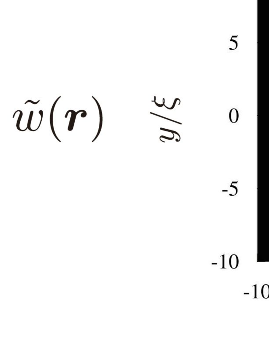
Figure 1: Spatial dependences of the amplitude of wave functions, scalar potential, and energy dissipation rate: (a1) $|\psi_{0}|$, (a2) $|\psi_{k}|$, (a3) $|\psi_{v}|$, (a4) $|\psi_{kv}|$; (b1) $\tilde{\varphi}_{0}$, (b2) $\tilde{\varphi}_{k}$, (b3) $\tilde{\varphi}_{v}$, (b4) $\tilde{\varphi}_{kv}$; (c1) $\tilde{w}_{0}$, (c2) $\tilde{w}_{k}$, (c3) $\tilde{w}_{v}$, (c4) $\tilde{w}_{kv}$. We have chosen $\bm{v}_{\rm L}=v_{\rm L}\hat{\bm{x}}$ and used $u=1$ (i.e. $\ell_{E}=\xi$). The system size is $L\times L$ with $L=40\xi$ and the number of mesh is $N_{L}\times N_{L}$ with $N_{L}=300$.

Figures 1(a1–4) shows the spatial dependences of the amplitudes of gap functions. The originally circular shape in Fig. 1(a1) is modified by $K$ and $v_{\rm L}$, and six-fold and two-fold patterns appear in Figs. 1(a2) and (a3), respectively. The more complex pattern is seen in the higher-order contribution $\psi_{kv}$ [Fig. 1(a4)]. The scalar potentials are also shown in Figs. 1(b1–4). The dipolar field is generated in $\varphi_{0}$ which causes the electric field inside the normal core. We note that the dimensionless $\tilde{\varphi}_{0}$ is $O(1)$ but the scalar potential $\varphi_{0}$ is $O(v_{\rm L})$ contribution. Then $\varphi_{v}$ shown in Fig. 1(b3) is an $O(v_{\rm L}^{2})$ contribution, having the quadrupolar distribution. The situation is further modified in the presence of the cubic term as in Figs. 1(a2) and (a4). We show in Figs. 1(c1–4) the energy dissipation rate as a function of spatial coordinates. The dissipation occurs in the region with $r\lesssim\ell_{E}$ as shown in Fig. 1(c1) (note that $W_{0}$ is an $O(v_{\rm L}^{2})$ contribution). This also applies at higher orders shown in Figs. 1(c2–4), where the spatial anisotropy is introduced.

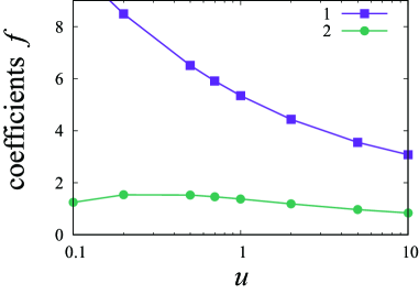
Figure 2: Parameter $u$ dependence of the friction force coefficients defined in Eq. (116). The system size and number of spatial mesh are same as Fig. 1.

We are also interested in the parameter $u=\xi^{2}/\ell_{E}^{2}$ dependence of the physical quantities. Figure 2 shows the force coefficients $f_{1}$ and $f_{2}$ as a function of $u$. For the larger $u$, meaning shorter electric-field penetration length, the value of $f_{1}$ becomes smaller. This is because the region where the dissipation occurs shrinks to make a weaker friction force. The value of $f_{2}$ at sufficiently large $u$ also becomes small due to the same reason as $f_{1}$. On the other hand, $f_{2}$ at small $u$ decreases in contrast with $f_{1}$. While the reason for the behavior is not easily understood in an intuitive way, in any case we have here confirmed that the coefficients of $f_{1}$ and $f_{2}$ are order of unity in the experimentally relevant regime with $u\sim 1$.

III.2.3 Flux-flow conductivity

Using the relation $\bm{E}_{0}=\bm{B}\times\bm{v}_{\rm L}$ for an electric field generated by the motion of the magnetic flux, which is derived from the Josephson relation, we obtain the electrical conductivity as

$$\bm{j}_{{\rm unif}} =\frac{\Gamma|\Delta_{\infty}|^{2}}{\Phi_{0}B_{z}}\left[f_{1}+\frac{f_{2}\Gamma K}{|\alpha|^{2}\xi^{4}B_{z}}\begin{pmatrix}E_{0x}&-E_{0y}\\ -E_{0y}&-E_{0x}\end{pmatrix}\right]\bm{E}_{0}$$ (118)

$$=\sigma_{1\mathrm{v}}\bm{E}_{0}+\sigma_{2\mathrm{v}}\bm{F}(\bm{E}_{0}),$$ (119)

where the vector $\bm{F}$ is same as that in Eq. (59). To express the flux-flow conductivity in terms of normal conductivity, we use the electric field penetration depth $\ell_{E}$ and the upper critical field given by $B_{c2}=\Phi_{0}/2\pi\xi^{2}$. Then the conductivities are given by

$$\sigma_{1\mathrm{v}} =\frac{uf_{1}(u)}{4\pi}\sigma_{n}\frac{B_{c2}}{B_{z}},$$ (120)

$$\sigma_{2\mathrm{v}} =\frac{uf_{2}(u)}{4\pi}\sigma_{n}\frac{B_{c2}\Gamma K}{\gamma^{2}B_{z}^{2}}.$$ (121)

The $\gamma$-value from nonreciprocal vortex dynamics is given by

$$\gamma_{\rm S}^{\mathrm{v}} =\frac{\sigma_{2\mathrm{v}}}{\sigma_{1\mathrm{v}}^{2}B_{z}W}=\frac{4\pi f_{2}(u)}{uf_{1}(u)^{2}}\cdot\frac{\Gamma K}{\gamma^{2}\sigma_{n}B_{c2}B_{z}W}.$$ (122)

This expression does not depend on $B_{z}$ since $K$ is proportional to $B_{z}$ due to the Zeeman effect. We note that the parameters $\sigma_{n}$, $\gamma$ and $K$ are in general dependent on the purity of the sample (see Appendix B).

Let us compare this result with the $\gamma$-value ($\gamma_{\rm S}^{\mathrm{f}}$) from superconducting fluctuation for $T\gtrsim T_{0}$ Wakatsuki . Noting $u\sim 1$, the ratio is estimated by

$$\frac{\gamma_{\rm S}^{\mathrm{v}}}{\gamma_{\rm S}^{\mathrm{f}}} \sim\frac{T_{0}^{2}}{E_{\rm F}(T_{0}-T)}.$$ (123)

Thus we obtain the same conclusion as the extended Bardeen-Stephen approach in Sec. III A 2.

III.3 Ratchet motion of vortex

As discussed above, for $T<T_{0}$ and in the presence of the finite out of plane magnetic field, the motion of quantum vortices penetrating the superconductor gives a dominant contribution to the voltage drop. Here we consider another effect for vortex dynamics. In the superconductor without inversion center, vortices driven by the external charge current feel an asymmetric pinning potential acting on them (ratchet effect). This effect has been proposed to control the vortices in superconductors Lee99 ; Villegas03 ; Villegas05 . New perspective here is that the vortex ratchet effect naturally appears as a consequence of disorders in noncentrosymmetric system, which is distinct from the previously discussed artificially developed inversion-broken environment. In this section, we analyze the classical motion of vortices under the asymmetric periodic potential and discuss the nonreciprocal transport there. The relevant parameters such as potential height and its spatial periodicity are estimated from pinning properties such as a magnitude of the critical current density where the vortices are depinned. The relation to the recent experimental results Wakatsuki ; Saito_private will also be discussed in Sec. IV C 2.

The classical equation of motion of the vortices in the diffusive limit is modeled as

$$\eta\frac{\mathrm{d}x}{\mathrm{d}t}=-\frac{\partial U}{\partial x}+F-\sqrt{2\eta T}\xi(t),$$ (124)

with $U$ being the pinning potential, which we here assume to be periodic for simplicity; $U(x+L)=U(x)$, and $F$ is the uniform force. The last term is the Langevin force with zero mean and unit dispersion (Gaussian white noise). $\eta$ is the viscous friction coefficient, and $T$ is the temperature. By solving the corresponding Fokker-Planck equation

$$\frac{\partial p}{\partial t}=\frac{1}{\eta}\frac{\partial}{\partial x}\left[\left(\frac{\partial U}{\partial x}-F\right)p+T\frac{\partial p}{\partial x}\right],$$ (125)

for the distribution function $p(x,t)$, we obtain the steady velocity of the vortex after long time expressed as Reimann

$$v_{\rm L}=\frac{L}{\beta\eta}\frac{1-e^{-\beta FL}}{\int_{0}^{L}dy\ I_{0}(y)e^{-\beta Fy}},$$ (126)

where we have introduced

$$I_{0}(y)=\int_{x_{0}}^{x_{0}+L}dx\ e^{\beta\left[U(x)-U(x-y)\right]},$$ (127)

with $\beta=1/T$ being the inverse temperature. We can choose $x_{0}$ arbitrarily due to the periodicity of the potential. Potential is called symmetric when there exists certain choice of $x_{0}\in\left[0,L\right)$ such that $U(x)=U(x_{0}-x)$ is satisfied. Here, we can choose $x_{0}=0$ by shifting the $x$ coordinate. By using the evenness and the periodicity of the potential, we can easily prove $v_{\rm L}(-F)=-v_{\rm L}(F)$ which show the absence of the nonreciprocal transport.

For asymmetric potentials, the situation is different. The velocity $v$ is expanded with respect to the force $F$ as

$$v_{\rm L} =q_{1}F+q_{2}F^{2}+O\left(F^{3}\right),$$ (128)

where the coefficients are

$$q_{1} =\frac{L}{\beta\eta}\frac{\beta L}{\int_{0}^{L}dy\ I_{0}(y)},$$ (129)

$$q_{2} =\frac{L}{\beta\eta}\frac{\beta^{2}L\int_{0}^{L}dy\left(y-\frac{L}{2}\right)I_{0}(y)}{\left[\int_{0}^{L}dy\ I_{0}(y)\right]^{2}},$$ (130)

where $q_{2}$, nothing but a hallmark of the nonreciprocal transport, survives only for asymmetric potentials as discussed above.

Hereafter, we adopt the fully asymmetric periodic potential for simplicity

$$U(x)=U_{0}\ \mathrm{saw}\left(\frac{x}{L}\right)=U_{0}\frac{x}{L}\quad(\mathrm{mod}\ L),$$ (131)

by using so-called sawtooth function. $U_{0}(>0)$ is the height of the pinning potential. In this potential, the steady velocity is calculated as

$$v_{\rm L}=\frac{1}{\beta\eta L}\frac{\beta^{2}(U_{0}-FL)^{2}}{\beta FL-\beta U_{0}-\sinh(\beta U_{0})+(\cosh(\beta U_{0})-1)\coth\left(\frac{\beta FL}{2}\right)}=q_{1}F+q_{2}F^{2}+O\left(F^{3}\right),$$ (132)

with the response coefficients

$$q_{1} =\frac{1}{2\eta}\frac{\beta^{2}U_{0}^{2}}{\cosh(\beta U_{0})-1}=\begin{cases}\displaystyle\frac{1}{\eta}-\frac{\beta^{2}U_{0}^{2}}{12\eta}&(\beta U_{0}\rightarrow 0)\\[11.38109pt] \displaystyle\frac{\beta^{2}U_{0}^{2}}{\eta}e^{-\beta U_{0}}&(\beta U_{0}\rightarrow\infty)\end{cases},$$ (133)

and

$$q_{2} =\frac{L\beta}{4\eta}\frac{\beta^{3}U_{0}^{3}+\beta^{2}U_{0}^{2}\sinh(\beta U_{0})+4\beta U_{0}-4\beta U_{0}\cosh(\beta U_{0})}{(\cosh(\beta U_{0})-1)^{2}}$$

$$=\begin{cases}\displaystyle\frac{L}{\eta}\frac{\beta^{4}U_{0}^{3}}{360}&(\beta U_{0}\rightarrow 0)\\[11.38109pt] \displaystyle\frac{L}{\eta}\frac{\beta^{3}U_{0}^{2}}{2}e^{-\beta U_{0}}&(\beta U_{0}\rightarrow\infty).\end{cases}.$$ (134)

Since the voltage drop originating from the motion of vortices is $V=B_{z}L_{x}v_{\rm L}$ and the force acting on vortices is $F=\frac{\phi_{0}}{W}I$, we can calculate the coefficients in current-voltage relation [Eq.(4)] as $a_{1}(B_{z},T)=\phi_{0}\frac{L_{x}}{W}B_{z}q_{1}(T)$ and $a_{2}(B_{z},T)=\phi_{0}^{2}\frac{L_{x}}{W^{2}}B_{z}q_{2}(T)$, both of which are proportional to $B_{z}$. The nonreciprocal $\gamma^{\prime}$ parameter defined as $R=R_{0}(1+\gamma^{\prime}I)$ with $V=RI$ is expressed as

$$\gamma^{\prime} =\frac{q_{2}}{q_{1}}\frac{\phi_{0}}{W}=\frac{\phi_{0}L}{W}\frac{U_{0}^{2}\beta^{2}+\beta U_{0}\sinh(\beta U_{0})-4\cosh(\beta U_{0})+4}{4U_{0}\sinh^{2}\left(\frac{\beta U_{0}}{2}\right)}$$

$$=\begin{cases}\displaystyle\frac{\phi_{0}L}{W}\frac{\beta^{4}U_{0}^{3}}{360}&(\beta U_{0}\rightarrow 0)\\[11.38109pt] \displaystyle\frac{\phi_{0}L}{W}\frac{\beta}{2}&(\beta U_{0}\rightarrow\infty)\end{cases},$$ (135)

which monotonically decrease as raising temperature. Note that the exponential temperature dependence vanishes for the $\gamma$-value.

In this calculation, we have neglected the vortex-vortex interaction. This assumption is justified for small magnetic field where the vortices are dilute enough. We also note that the ratchet effect is active for trigonal symmetry, but is not relevant for the systems with $C_{\infty}$ and hexagonal symmetries where no ratchet potential is present. In the latter cases, the effect from asymmetric spin-orbit coupling plays the more dominant role.

IV Discussion

Here we discuss expected noreciprocal charge signals in 2DNS. Table 1 summarizes the nonreciprocal $I$-$V$ characteristics in Rashba superconductors, TI surface and TMD for both above and below transition temperature. The magnetic fields are applied parallel to the two-dimensional plane for Rashba and TI based systems, and applied perpendicular to the layer for TMD. While the other configurations can in principle be possible, the information of this paper gives a firm basis to explore the further properties. Below we discuss each system separately.

IV.1 Rashba superconductors

Here we consider the typical $\gamma$-value for Rashba superconductors. With electron or hole doping, the Fermi energy can be tuned and the behavior is dependent on the sign of $E_{\rm F}$. Let us begin with the $E_{\rm F}<0$ case. In this case, the normal contribution to $\gamma$-value becomes finite as shown in Ref. IdeueHamamoto, (see also Table 1). The typical values for BiTeBr have been estimated IdeueHamamoto by using the effective mass h$m=0.15m_{e}$, the Rashba parameter $\alpha=2.00$ eV Å, and the g-factor $g=60$. In the normal state with $E_{\rm F}=-0.01$ eV, the amplitude of the magnetochiral anisotropy is estimated as $W\gamma_{\rm N}\simeq 2\times 10^{-5}$ ${\rm T^{-1}A^{-1}m}$.

The system crossovers into the paraconductivity region with approaching to the mean-field transition temperature $T_{0}$ from above. Here, as discussed in Sec. II.1, the parity mixing contribution becomes irrelevant and the cubic term in GL free energy instead becomes dominant. The paraconductivity is then given by Eq. (37). The ratio between normal and superconducting states is given by $\gamma_{\rm S}/\gamma_{\rm N}\sim E_{\rm F}/T_{0}$, and thus the nonreciprocal signal is strongly enhanced by the appearance of a small energy scale $T_{0}$ for superconductors.

The fluctuation contribution above $T_{0}$ further crossovers to vortex contribution at lower temperatures than $T_{0}$. Below $T_{0}$, the pair amplitude sufficiently develops and the free vortices, which are generated thermally above KT transition temperature in the present system, start to play an important role for transport phenomena. For $E_{\rm F}<0$ case, the cubic term effectively renormalizes superfluid density under the transport current as discussed in Sec. III.1. As a result, the friction force and KT transition temperature are modified and have different values depending on the direction of source currents. The former causes the characteristic temperature dependence in the $\gamma$-value as $\gamma_{\rm S}\propto(T_{0}-T)^{-1}$ near $T_{0}$ $(>T_{\rm KT})$. Note that this expression smoothly connects to the fluctuation contribution for $T>T_{0}$, and does not show divergence in reality. On the other hand, the modification of the KT transition temperature shows the divergent $\gamma$-value as $\gamma_{\rm S}\propto(T-T_{\rm KT})^{-3/2}$ near the KT transition point. For $T<T_{\rm KT}$, vortex and antivortex are bound, and the linear transport coefficient finally vanishes. The third-order term with $a_{3}$ then becomes the relevant one in the current-voltage relation. The nonreciprocity is reflected in the higher order term with $a_{4}$ in this case. More detailed investigation of these higher-order contributions remains to be clarified in the future.

Now, we switch our focus to the $E_{\rm F}>0$ case. Although the normal state contribution to $\gamma$-value is absent in this situation IdeueHamamoto , the paraconductivity is finite. There are two contributions to paraconductivity: one from parity mixing and the other from $\bm{q}$-cubic term in the GL theory. Here, as the ratio is calculated in Eq. (38), the parity-mixing contribution in Eq.(23) is much larger than the other. The $\gamma$-value in this case has been estimated in Ref. WakatsukiNagaosa for BiTeBr with superconducting proximity effects. On the othe hand, the LaAlO₃/SrTiO₃ interface Reyren ; Caviglia ; Maniv ; Herranz is also a typical two-dimensional Rashba superconductor. Its carrier density is given by $n\sim 10^{13}\mathrm{cm}^{-2}$, spin–orbit field is $B_{\mathrm{SO}}=\frac{m^{2}\alpha^{2}}{|e|}\sim 1\mathrm{T}$, the Debye temperature is $T_{\mathrm{D}}\sim 400\mathrm{K}$, and the mean-field transition temperature is $T_{0}\sim 100\mathrm{mK}$. If we assume $r_{\mathrm{t}}=0.1$ and the typical sample width $W=10^{-6}$m, the $\gamma$-value is estimated as $\gamma_{\mathrm{S}}\sim 8\times 10^{4}\mathrm{T^{-1}A^{-1}}$, which is much larger than the previous studies Rikken1 ; Rikken2 ; Pop ; Krstic ; Rikken3 .

At lower temperature below $T_{0}$, the vortex contribution dominates over the paraconductivities. For $E_{\rm F}>0$ case, the two-component gap parameter need to be considered for vortex dynamics. While detailed studies remain unexplored, the vortex contribution should be present and is expected to cause a singular behavior around the KT transition point as in the $E_{\rm F}<0$ case.

IV.2 TI surface

We here discuss the surface of topological insulators plus superconducting proximity effect. The Hamiltonian has the $\bm{k}$-linear term, but the nonreciprocal charge transport is absent with this term only. We have thus considered the two more terms to generate the nonreciprocity: parabolic term and hexagonal warping term. Let us first consider the contribution from parabolic term based on Eq.(43). The functional forms of the $\gamma$-values are listed in Table 1. The ratio between normal and superconducting states is given by $\gamma_{\rm S}/\gamma_{\rm N}\sim E_{\rm F}/T_{0}$. Hence, the nonreciprocal transport signal is enhanced in superconducting state. To estimate the typical value, we use the expression in Eq. (43) with $\hbar$, $k_{\mathrm{B}}$, and $\mu_{\mathrm{B}}$ recovered. If we assume $v_{\rm F}=2.84$ eVÅ and $\frac{1}{2m}=41.1$ eVŲ in Bi₂Te₃ Kim , and $E_{\mathrm{F}}=0.1$ eV, $T_{0}=10$ K, and $W=100$ $\mu$m as typical values, we obtain $\gamma_{\mathrm{S}}\approx 0.33$ $\mathrm{A}^{-1}\mathrm{T}^{-1}$. On the other hand, the contribution from the hexagonal warping is given in Eq. (53), and is here also estimated. Assuming the same parameters above and $\sqrt{\lambda}=250$ eVų in Bi₂Te₃ Kim ; Fu , we obtain $\gamma_{\mathrm{S}}\approx 0.11$ $\mathrm{A}^{-1}\mathrm{T}^{-1}$. Therefore, the amplitude is comparable to that by the parabolic term.

At lower temperatures, the vortex contribution becomes dominant as in the Rashba superconductors. Since the magnetic field is applied along the two-dimensional plane and there is the cubic term in GL free energy, the behavior is essentially same as the Rashba superconductors with $E_{\rm F}<0$. Namely, the thermally generated vortex in the $T_{\rm KT}<T\lesssim T_{0}$ region creates the characteristic magnetochiral anisotropy in the forms $\gamma_{\rm S}\propto(T_{0}-T)^{-1}$ for $T\rightarrow T_{0}$ and $\gamma_{\rm S}\propto(T-T_{\rm KT})^{-3/2}$ for $T\rightarrow T_{\rm KT}$. We note that the above transport coefficients are written in the form $V=a_{1}I(1+\gamma BI)$, i.e. the magnetic field $B$ enters only with $\gamma$-value. As shown below, however, the situation can qualitatively change if the magnetic field is applied perpendicular to the plane.

IV.3 TMD

IV.3.1 Paraconductivity and intrinsic vortex-flow contribution

We estimate the physical quantities of the clean MoS₂. Let us begin with the normal contribution well above $T_{0}$. This system has a valley degrees of freedom, whose contribution to the normal $\gamma$-value per valley is listed in Table 1. With the situation in MoS₂, however, the $\gamma$-value for each valley has different sign and vanishes if we sum up both the contributions Wakatsuki . Near $T_{0}$, the paraconductivity contribution is developed as given in Eq. (60). Using $2m\lambda/\hbar^{2}=-0.49\AA$ and $\Delta_{\rm SO}\simeq 7.5$ meV, and $T_{0}=8.8$ K for monolayer MoS₂, the $\gamma$-value from the superconducting fluctuation reaches $\gamma_{\rm S}\simeq 250{\rm T^{-1}A^{-1}}$ for the sample width $W\simeq 3\mu{\rm m}$, as shown in Ref. Wakatsuki, .

Below $T_{0}$, here again the vortex contribution becomes relevant for the $\gamma$-value, but the situation is different from the Rashba and TI based systems with KT transition. Namely, the vortices with the same vorticity are induced by the out-of-plane magnetic field and the KT transition is washed away for $B\neq 0$. As a result, the number of vortices are determined by the external field $B$, and the ordinary resistivity $a_{1}(B)$ is proportional to $B$. We reflect this situation by denoting $I$-$V$ characteristic as $V=a_{1}^{\prime}BI+a_{2}(B)I^{2}$. As for the coefficient $a_{2}(B)$, there are two types of contributions. One is from the $\bm{q}$-cubic term in the GL free energy and $a_{2}$ is proportional to $B^{2}$. The other is from the ratchet potential for vortices, and $a_{2}\propto B$ is satisfied. Thus the $B$ dependence of $a_{2}$ clearly distinguishes the underlying mechanism to generate nonreciprocal charge transport. Since the latter effect is discussed in detail in the next subsection, we here focus on the cubic-term contribution. The $I$-$V$ relation is then written as $V=a_{1}^{\prime}BI(1+\gamma_{\rm S}BI)$.

As discussed in Sec. III.1, the $\bm{q}$-cubic term in GL free energy effectively renormalizes the superfluid density. We have applied the generalized Bardeen-Stephen approach to this system: the force balance between driving (Magnus) force and viscous force acting on the vortex is considered. The nonreciprocity enters in the friction force through the anisotropically renormalized superfluid density. We have then found that the $\gamma$-value from vortex dynamics is given by $\gamma_{\rm{S}}^{\rm v}=\gamma_{\rm{S}}^{\rm f}\times\frac{T_{0}^{2}}{E_{\rm F}(T-T_{0})}$ with $\gamma_{\rm S}^{\rm f}$ being the superconducting fluctuation contribution, which has a large value near the mean-field transition temperature $T_{0}$. Here the temperature dependence enters through the unrenormalized superfluid density which behaves as $n_{s}\propto(T_{0}-T)$. Such behavior has further been justified by the TDGL approach as demonstrated in Sec. III B. If the results are extrapolated to zero temperature, we get $\gamma^{\rm v}_{\rm{S}}/\gamma^{\rm f}_{\rm{S}}=T_{0}/E_{\rm F}$. Since the magnitude of the paraconductivity contribution is roughly given by $\gamma_{\rm S}^{\rm f}\sim 10^{2}{\rm T^{-1}A^{-1}}$ as discussed above, the order of magnitude for the vortex contribution is $\gamma_{\rm S}^{\rm v}\sim 1{\rm T^{-1}A^{-1}}$ in the low-temperature limit. This is much smaller than the observed values at low $T$ in the monolayer MoS₂ Wakatsuki , and hence we need another mechanism to account for the experimental results.

IV.3.2 Ratchet effect of vortex flow

We now consider the nonreciprocal transport from ratchet effect of vortex dynamics based on Eq. (135). Phenomenological parameters such as periodicity $L$ of the pinning potential, friction coefficient $\eta$, and potential height $U_{0}$ are estimated for MoS₂ using experimental data. The parameter $L$ is determined from the mean distance of pinning centers. This can be estimated from pinning-depinning transition point in the magnetoresistance measurement, that is about $B_{z}\simeq 0.2\mathrm{T}$ Saito_private At this transition point, all the pinning centers are assumed to be filled with vortices. The total flux is $B_{z}L_{x}W=N_{\rm v}\Phi_{0}$ then the vortex number density is $n_{\rm v}=N_{\rm v}/(L_{x}W)=B_{z}/\Phi_{0}$. Thus the mean distance between vortices is

$$L\sim\frac{1}{\sqrt{n_{\rm v}}}=\sqrt{\frac{\Phi_{0}}{B_{z}}}\sim 10^{-7}\mathrm{m}.$$ (136)

The parameter $\eta$ is estimated by the normal state resistivity. In the absence of the pinning potentials, $(U_{0}=0)$, the $I$-$V$ characteristic becomes $v_{\rm L}=F/\eta$ or

$$V=B_{z}v_{\rm L}L_{x}=B_{z}\frac{F}{\eta}L_{x}=B_{z}\frac{\Phi_{0}}{\eta}\frac{L_{x}}{W}I=RI,$$ (137)

in the ohmic region. The resistivity $R=B_{z}\frac{\Phi_{0}}{\eta}\frac{L_{x}}{W}$ should be same as the normal state resistivity $R_{n}$ when $B_{z}=B_{\rm c2}\simeq 0.1\ \mathrm{T}$. Thus, the parameter $\eta$ is estimated as

$$\eta=\frac{\Phi_{0}B_{\rm c2}}{R_{n}}\frac{L_{x}}{W}=\frac{\Phi_{0}B_{\rm c2}}{R_{n}}\sim 10^{-18}\ \mathrm{kg/s},$$ (138)

with $R_{n,{\rm sheet}}\simeq 300\ \mathrm{\Omega}$ Saito .

The parameter $U_{0}$, the height of the pinning potential of the superconducting vortex, is estimated by the plateau of $R$-$B$ curve in weak $B$ region. The plateau disappears for $j_{\mathrm{sheet}}>j_{\rm c}\simeq 3\mathrm{A/m}$ Saito_private , where $j_{\rm c}$ is the critical current density for vortex depinning. Depinnig transition occurs when the pinning potential is well tilted by the external force, namely;

$$U_{0}\sim FL=j_{\mathrm{sheet}}\Phi_{0}L\simeq 4\ \mathrm{meV}.$$ (139)

Another estimation of $U_{0}$ is from the thermodynamic upper critical field. The vortex energy per unit volume is $B_{c2}^{2}/(2\mu_{0})$. When the vortex has the overlap with normal core in the pinning center, the energy reduces. By using $B_{c2}\simeq 0.1\ \mathrm{T}$ Saito , we obtain

$$U_{0}\sim\frac{B_{c2}^{2}}{2\mu_{0}}\pi\xi^{2}c_{z}\simeq 5\ \mathrm{meV},$$ (140)

with $\xi\simeq 8\mathrm{nm}$ and $c_{z}\simeq 1\mathrm{nm}$ being the in-plane coherence length (normal core radius) and the lattice constant in the thickness direction, respectively. These two estimations are very consistent. We note $U_{0}\simeq 5\ \mathrm{meV}\simeq 58\ \mathrm{K}$ is much larger than the transition temperature therefore low temperature limit, $\beta U_{0}\gg 1$, is the realistic situations in MoS₂.

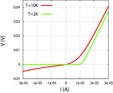
Figure 3: $I$-$V$ characteristic curve for the monolayer MoS₂ at $T=10$K and $T=2$K.

Calculated $I$-$V$ characteristic curve is shown in Fig. 3, which displays a strong rectification behavior even at a measurable temperature. For larger current such that $U_{0}<FL$, the expansion with respect to $F$ or equivalent to $I$ is no longer valid. In this regime, the $I$-$V$ characteristics are strongly non-linear and hence the higher harmonics becomes relevant. At the critical current where $U_{0}=F_{c}L$, the potential becomes a multi-step function and therefore the velocity begins to grow rapidly.

The temperature dependence of $\gamma$-value at low $T$ is given by $\gamma_{\rm S}^{\prime}\propto 1/T$ for the ratchet mechanism according to Eq. (135) in the $U_{0}\gg T$ limit. With the original expression in Eq. (135), the estimated $\gamma$-values for the sample size $L_{x}Wc_{z}=3{\rm\mu m}\times 3{\rm\mu m}\times 1{\rm nm}$ are given by $\gamma_{\rm S}^{\prime}\simeq 8\times 10^{5}{\rm A^{-1}}$ at $T=10$K and $\gamma_{\rm S}^{\prime}\simeq 1\times 10^{6}{\rm A^{-1}}$ at $T=2$K. Although these magnitudes are much larger than the ones in the experimental observation Wakatsuki , we can obtain the more close values by controlling the spatial asymmetry in the sawtooth potential. Namely, by tuning the potential from the asymmetric case in Eq. (131) to symmetric case continuously, the $\gamma$-value is monotonically decreased down to zero.

At sufficiently low temperatures, on the other hand, the quantum nature of the vortices plays an important role. In this case the wave character of vortices appears, which will modify the above physical picture. This point remains to be explored in the future.

V Summary and conclusions

We have theoretically investigated the nonreciprocal charge transports in the two-dimensional superconductors without inversion symmetry. We have taken the concrete examples such as the Rashba superconductors and topological insulator surface with in-plane magnetic fields, and the monolayer transition metal dichalcogenide (MoS₂) with out-plane magnetic field. The nonreciprocal properties of superconductors are reflected in the $I$-$V$ characteristics with the form $V=a_{1}I+a_{2}I^{2}+a_{3}I^{3}+a_{4}I^{4}$, and the odd-order terms represent the nonreciprocal responses. These coefficients are clarified in the temperature range both above and below the mean-field transition temperature. Table 1 summarizes our obtained results.

The nonreciprocal transport signals in the normal regions well above the mean-field transition temperature $T_{0}$ crossover into superconducting fluctuation contribution (paraconductivity). We have newly investigated the topological insulator based systems which have cubic term in the GL free energy, in addition to the previously investigated Rashba superconductors and transition metal dichalcogenide. The $\gamma$-values for all the systems are much enhanced compared to the normal state, which is attributed to the appearance of the small energy scale $T_{0}$ ($\ll E_{\rm F}$). The ratio of $\gamma$-values between normal and superconducting fluctuation region is in general written as $(E_{\rm F}/T_{0})^{m}$ with $m\geq 1$ being an integer depending on the system.

Below $T_{0}$, the amplitude of the superconducting order parameters is developed and only the phase degrees of freedom are left. Then the vortex dynamics plays an important role for $T\lesssim T_{0}$. There are two different kinds of vortex behaviors. First, for systems with in-plane magnetic fields, the vortices are thermally generated and are bound below the Kosterlitz-Thouless transition temperature $T_{\rm KT}$. Due to the inversion symmetry breaking in the system, the friction force and the number of vortices for $T_{\rm KT}<T<T_{0}$ are different depending on the direction of external uniform current, to produce the nonreciprocal charge transport. These effects have effectively been described by the renormalization of the superfluid density. The $\gamma$-value, which is defined by $V=a_{1}I(1+\gamma BI)$ as in the fluctuation regime, is identified to have the temperature-dependent forms $\gamma\propto(T_{0}-T)^{-1}$ near $T_{0}$ and $\gamma\propto(T-T_{\rm KT})^{-3/2}$ near $T_{\rm KT}$, which originate from the modified friction coefficient and the modified KT transition temperature, respectively. Accordingly, we expect the two-peak structure of the temperature dependence of the $\gamma$-value in this case.

For the system with out-plane magnetic field, the number of vortices with a same vorticity is determined by the strength of the external field $B$ and the Kosterlitz-Thouless transition does not exist. The nonreciprocal signal $\gamma$ is now characterized by the $I$-$V$ relation with the form $V=a_{1}^{\prime}BI(1+\gamma BI)$. The renormalization of superfluid density works also for this system, and we have derived the modified friction force for moving vortices and the corresponding $\gamma$-value has the form $\gamma\propto(T_{0}-T)^{-1}$. This phenomenological approach is further justified by the time-dependent Ginzburg-Landau theory. On the other hand, we have also investigated the other effect with ratchet potential for vortices. Here the magnetic field plays a role only for creating the vortex, and then the $\gamma$-value is characterized by the relation $V=a_{1}^{\prime}BI(1+\gamma_{\rm S}^{\prime}I)$. We have considered one dimensional motion driven by the external transport current in the sawtooth potential, and have found that the resultant signal $\gamma^{\prime}$ can have a comparable value with the experiments in MoS₂.

We have thus systematically clarified the characteristic transport properties for two-dimensional noncentrosymmetric superconductors. The knowledge of this paper is useful for the further exploration of nonreciprocal phenomena in superconductors both theoretically and experimentally.

Appendix A Derivation of the Ginzburg-Landau free energy

Following Ref. BauerSigrist, , we derive the GL free energy for the model in Eq. (7). Especially, we focus on the case where the Fermi energy is on the conduction band. The free energy is given by

$$F=\int\frac{d^{2}\bm{q}}{\left(2\pi\right)^{2}}\left[\frac{1}{g}-T\sum_{\omega_{n}}\int\frac{d^{2}\bm{k}}{\left(2\pi\right)^{2}}G\left(\bm{k},i\omega_{n}\right)G\left(-\bm{k}+\bm{q},-i\omega_{n}\right)\right]\left|\Psi_{\bm{q}}\right|^{2},$$ (141)

with $G\left(\bm{k},i\omega_{n}\right)=\left(i\omega_{n}-\xi_{\bm{k}}\right)^{-1}$ being the Matsubara Green’s function. The product of the Green functions is simplified as

$$\int\frac{d^{2}\bm{k}}{\left(2\pi\right)^{2}}G\left(\bm{k},i\omega_{n}\right)G\left(-\bm{k}+\bm{q},-i\omega_{n}\right)$$

$$=\int\frac{d^{2}\bm{k}}{\left(2\pi\right)^{2}}\frac{1}{i\omega_{n}-\xi_{\bm{k}}}\frac{1}{-i\omega_{n}-\xi_{-\bm{k}+\bm{q}}}$$

$$=-\int\frac{d^{2}\bm{k}}{\left(2\pi\right)^{2}}\frac{1}{i\omega_{n}-\xi^{0}_{\bm{k}}-\Omega_{1}\left(\bm{k}\right)}\frac{1}{i\omega_{n}+\xi^{0}_{\bm{k}}+\Omega_{2}\left(\bm{k},\bm{q}\right)},$$ (142)

where

$$\xi^{0}_{\bm{k}} =\frac{\bm{k}^{2}}{2m}+\alpha|\bm{k}|-E_{\mathrm{F}},$$ (143)

$$\Omega_{1}\left(\bm{k}\right) =\xi_{\bm{k}}-\xi^{0}_{\bm{k}},$$ (144)

$$\Omega_{2}\left(\bm{k},\bm{q}\right) =\xi_{-\bm{k}+\bm{q}}-\xi^{0}_{\bm{k}}.$$ (145)

We first integrate by $\xi^{0}_{\bm{k}}$

$$-\int\frac{d^{2}\bm{k}}{\left(2\pi\right)^{2}}\frac{1}{i\omega_{n}-\xi^{0}_{\bm{k}}-\Omega_{1}\left(\bm{k}\right)}\frac{1}{i\omega_{n}+\xi^{0}_{\bm{k}}+\Omega_{2}\left(\bm{k},\bm{q}\right)}$$

$$\approx-\nu_{1}\left<\int d\xi\frac{1}{i\omega_{n}-\xi-\Omega_{1}\left(\bm{k}\right)}\frac{1}{i\omega_{n}+\xi+\Omega_{2}\left(\bm{k},\bm{q}\right)}\right>_{\bm{k}}$$

$$=\pi\nu_{1}\left<\frac{1}{\left|\omega_{n}\right|+i\mathrm{sgn}\left(\omega_{n}\right)\Omega\left(\bm{k},\bm{q}\right)}\right>_{\bm{k}},$$ (146)

where $\left<\cdots\right>_{\bm{k}}$ is the momentum average over the Fermi surface. When we consider the surface state of topological insulator, which we describe here for simplicity, we only take the inner one of the two Fermi surfaces. The Fermi wavenumber is $k_{\mathrm{F1}}=-m\alpha+\sqrt{mE_{\mathrm{FR}}}$, and the density of states is $\nu_{1}=\frac{m}{2\pi}\left(1-\alpha\sqrt{m/E_{\mathrm{FR}}}\right)$. We have defined $\Omega\left(\bm{k},\bm{q}\right)=\frac{1}{2}\left(\Omega_{1}\left(\bm{k}\right)-\Omega_{2}\left(\bm{k},\bm{q}\right)\right)$. Therefore, the second term in Eq. (141) is

$$-\pi T\nu_{1}\sum_{\omega_{n}}\left<\frac{1}{\left|\omega_{n}\right|+i\mathrm{sgn}\left(\omega_{n}\right)\Omega\left(\bm{k},\bm{q}\right)}\right>_{\bm{k}}$$

$$\approx-\pi T\nu_{1}\sum_{\omega_{n}}\left<\frac{1}{\left|\omega_{n}\right|}-\frac{\Omega\left(\bm{k},\bm{q}\right)^{2}}{\left|\omega_{n}\right|^{3}}+\frac{\Omega\left(\bm{k},\bm{q}\right)^{4}}{\left|\omega_{n}\right|^{5}}\right>_{\bm{k}}$$

$$=-\nu_{1}\left[S_{1}\left(T\right)-S_{3}\left(T\right)\left<\Omega\left(\bm{k},\bm{q}\right)^{2}\right>+S_{5}\left(T\right)\left<\Omega\left(\bm{k},\bm{q}\right)^{4}\right>\right],$$ (147)

with $S_{k}\left(T\right)=\pi T\sum_{n}\left|\omega_{n}\right|^{-k}$. The function $S_{k}(T)$ is calculated as

$$S_{1}\left(T\right) =\log\frac{2e^{\gamma_{\mathrm{E}}}E_{\mathrm{c}}}{\pi T},$$ (148)

$$S_{3}\left(T\right) =\frac{7\zeta\left(3\right)}{4\left(\pi T\right)^{2}},$$ (149)

$$S_{5}\left(T\right) =\frac{31\zeta\left(5\right)}{16\left(\pi T\right)^{4}},$$ (150)

with $\gamma_{\mathrm{E}}$ being the Euler’s constant and $E_{\mathrm{c}}$ being the cutoff energy. Then, we calculate $\left<\Omega\left(\bm{k},\bm{q}\right)^{2}\right>$ and $\left<\Omega\left(\bm{k},\bm{q}\right)^{4}\right>$ up to $O\left(B_{y}\bm{q}^{4}\right)$. If we shift the momentum as $\bm{q}\rightarrow\bm{q}+\frac{2B_{y}m}{|\bm{k}|+m\alpha}\hat{\bm{x}}$, we find

$$\left<\Omega\left(\bm{k},\bm{q}\right)^{2}\right> =\frac{\left(k_{\mathrm{F1}}+m\alpha\right)^{2}}{8m^{2}}\bm{q}^{2}$$

$$\ \ +\frac{3\left(5k_{\mathrm{F1}}+3m\alpha\right)}{32mk_{\mathrm{F1}}\left(k_{\mathrm{F1}}+m\alpha\right)}B_{y}q_{x}\bm{q}^{2}+O\left(\bm{q}^{4}\right),$$ (151)

$$\left<\Omega\left(\bm{k},\bm{q}\right)^{4}\right> =O\left(\bm{q}^{4}\right).$$ (152)

This result is reasonable because the third order term in the momentum vanishes for $m\rightarrow\infty$. The case of the valence band $\left(E_{\mathrm{F}}<0\right)$ can be obtained in a similar manner, and we can show that the free energy is obtained by replacing $\alpha$ with $-\alpha$, $B_{y}$ with $-B_{y}$, $k_{\mathrm{F1}}=-m\alpha+\sqrt{mE_{\mathrm{FR}}}$ with $k_{\mathrm{F2}}=m\alpha-\sqrt{mE_{\mathrm{FR}}}$ and $\nu_{1}=\frac{m}{2\pi}\left(1-\alpha\sqrt{m/E_{\mathrm{FR}}}\right)$ with $\nu_{2}=\frac{m}{2\pi}\left(-1+\alpha\sqrt{m/E_{\mathrm{FR}}}\right)$. We can also derive the GL free energy for the model with the hexagonal warping [Eq. (50)] in the same way.

Appendix B Impurity effect in TMD

The effect of superconducting fluctuation is more prominent for dirty samples according to the Ginzburg-Levanyuk criterion LarkinVarlamov

$$|\epsilon|\lesssim\left[\frac{k_{\rm F}\xi_{0}}{(k_{\rm F}\xi)^{D}}\right]^{\frac{2}{4-D}},$$ (153)

where $\epsilon=(T-T_{0})/T_{0}$ is the reduced temperature, $D$ is the dimension of the system. $\xi$ is the coherence length for either clean or dirty samples. Here we consider the impurity effect on the GL equation with $\bm{q}$-cubic term originating from trigonal warping for MoS₂. To deal with the impurities, we take quasi-classical Green function method Kopnin_book . We introduce the normal and anomalous quasiclassical Green functions by $g(\hat{\bm{k}},i\omega_{n};\bm{r})$ and $f(\hat{\bm{k}},i\omega_{n};\bm{r})$, respectively, where $\hat{\bm{k}}$ is the unit vector in the direction of $\bm{k}$ on the warped Fermi surface and $\omega_{n}=(2n+1)\pi T$ is the fermionic Matsubara frequency. The gap equation is given by

$$\Delta(\bm{r})=\pi i\nu V^{\rm g}T\sum_{n}\langle f(\hat{\bm{k}},i\omega_{n};\bm{r})\rangle_{{\bm{k}}},$$ (154)

where the bracket means the average with respect to ${\bm{k}}$. $V^{\rm g}$ and $\nu$ are the attractive interaction parameter and density of states at the Fermi level, respectively. To derive the GL theory, we expand the right-hand side of Eq. (154). The terms without spatial derivatives are not affected by impurities, which is known as the Anderson theorem. Hence we only keep the linear term in $\Delta$ and consider spatial derivatives. With this condition we can use $g(\hat{\bm{k}},i\omega_{n};\bm{r})={\rm sgn\,}\omega_{n}$, since it does not have the linear term of $\Delta$. The anomalous Green function is described by the Eilenberger equation:

$$i\bm{v}(\hat{\bm{k}})\cdot\bm{\nabla}f+2i\omega_{n}f-2\Delta g+\frac{i}{\tau}(\langle g\rangle_{{\bm{k}}}f-\langle f\rangle_{{\bm{k}}}g)=0,$$ (155)

where $\bm{v}$ is the Fermi velocity. The self energy from impurities has been included by the self-consistent Born approximation. The Zeeman energy can be accounted for by the simple replacement $i\omega_{n}\rightarrow i\omega_{n}+B_{z}$, and we do not write this explicitly for the moment. Now we perform the gradient expansion as $f=f_{0}+f_{1}+f_{2}+f_{3}+\cdots$. The zeroth and first-order terms can be explicitly written as

$$\langle f_{0}\rangle_{{\bm{k}}} =f_{0}=\frac{\Delta{\rm sgn\,}\omega_{n}}{i\omega_{n}},$$ (156)

$$\langle f_{1}\rangle_{{\bm{k}}} =-\frac{i\langle\bm{v}\rangle_{{\bm{k}}}\cdot\bm{\nabla}f_{0}}{2i\omega_{n}},$$ (157)

where $\tilde{\omega}_{n}=\omega_{n}+\frac{1}{2\tau}{\rm sgn\,}\omega_{n}$. We conclude $\langle f_{1}\rangle_{{\bm{k}}}=0$ since $\langle\bm{v}\rangle_{{\bm{k}}}=0$ is satisfied. The higher-order terms can also be derived as

$$\langle f_{2}\rangle_{{\bm{k}}} =\frac{\langle(i\bm{v}\cdot\bm{\nabla})^{2}f_{0}\rangle_{{\bm{k}}}}{4i\omega_{n}i\tilde{\omega}_{n}},$$ (158)

$$\langle f_{3}\rangle_{{\bm{k}}} =-\frac{\langle(i\bm{v}\cdot\bm{\nabla})^{3}f_{0}\rangle_{{\bm{k}}}}{4i\omega_{n}(i\tilde{\omega}_{n})^{2}}.$$ (159)

$\langle f_{3}\rangle_{{\bm{k}}}$ can be finite if the system has a trigonal warping. To be compatible with the results in the previous sections, there are the relations

$$\langle(i\bm{v}\cdot\bm{\nabla})^{2}\rangle_{{\bm{k}}} =C_{2}\bm{\nabla}^{2},$$ (160)

$$\langle(i\bm{v}\cdot\bm{\nabla})^{3}\rangle_{{\bm{k}}} =iC_{3}\partial_{x}(\partial_{x}^{2}-3\partial_{y}^{2}).$$ (161)

The real constants $C_{2}$ and $C_{3}$ are determined to be consistent with the expressions in the clean limit which has already been obtained in Ref. Wakatsuki, .

We now replace $i\omega_{n}$ by $i\omega_{n}+B_{z}$ to include the Zeeman energy, and take the lowest order contribution of the external magnetic field $B_{z}$. We substitute these expressions into the gap equation. The coefficient $\gamma(\tau)$ of $\bm{q}$-square term and $K(\tau)$ of $\bm{q}$-cubic term in the GL equation, which are now dependent on the mean-free time $\tau$, are given by

$$\gamma(\tau)/\gamma(\infty)=\sum_{n}\frac{1}{|\omega_{n}|^{2}(|\omega_{n}|+\frac{1}{2\tau})}\left/\sum_{n}\frac{1}{|\omega_{n}|^{3}}\right.,$$ (162)

$$K(\tau)/K(\infty)=$$

$$\frac{1}{2}\sum_{n}\frac{1}{|\omega_{n}|^{2}(|\omega_{n}|+\frac{1}{2\tau})^{2}}\left(\frac{1}{|\omega_{n}|}+\frac{1}{|\omega_{n}|+\frac{1}{2\tau}}\right)\left/\sum_{n}\frac{1}{|\omega_{n}|^{5}}\right.,$$ (163)

to obtain the results with impurities. These factors can be used at any purity of samples and go to unity for the clean limit. The square coefficient here is not a new result which can be seen in e.g. Ref. Kim_book , and the cubic coefficient is first derived. Particularly for the $\gamma$-value, the ratio between dirty ($\tau T_{0}\ll 1$) and clean ($\tau T_{0}\gg 1$) limits is given by

$$\frac{\gamma^{\rm f}_{\rm S,dirty}}{\gamma^{\rm f}_{\rm S,clean}}\sim\tau T_{0},$$ (164)

for superconducting fluctuation contribution. For vortex flow contribution, on the other hand, the transport coefficients are dependent on $\sigma_{n}$ ($\simeq n_{e}e^{2}\tau/m$) and cannot be written in a simple way, but can be in general estimated from the above information.

Appendix C Effect of Landau level for paraconductivity in TMD

C.1 Formulation

We here extend the calculation for the paraconductivity in the low-field limit to the case in the presence of quartic term and magnetic field. The paraconductivity from superconducting fluctuations can be evaluated at arbitrary strength of the magnetic field by considering the Landau levels. Let us begin with the GL free energy

$$F =\int d^{2}\bm{r}\Psi^{*}\left[a+\frac{\bm{P}^{2}}{2m^{*}}+\Lambda B_{z}(P_{x}^{3}-3\overline{P_{x}P_{y}^{2}})\right]\Psi,$$ (165)

where $\bm{P}=-i\bm{\nabla}-e^{*}\bm{A}$ with $e^{*}=2e$ and $m^{*}=2m$. The quartic term with $|\Psi|^{4}$ can be effectively included in the square term by using the self-consistent harmonic approximation and is dropped here. We will explain this point later. The spatially averaged supercurrent is given in the simple form

$$J_{sx} =-|e^{*}|\int\frac{d^{2}\bm{r}}{\Omega}\Psi^{*}\left[\frac{1}{m^{*}}P_{x}+3\Lambda B_{z}(P_{x}^{2}-P_{y}^{2})\right]\Psi,$$ (166)

where $\Omega=\int d^{2}\bm{r}1$ is a two-dimensional system volume. The $y$-component can be constructed by symmetry and we do not consider here. We choose the vector potential as $A_{x}=-E_{x}t$ and $A_{y}=-E_{y}t+B_{z}x$. Now we expand the complex function $\Psi$ as

$$\Psi(\bm{r},t) =\sum_{kn}c_{kn}(t)e^{-iky}e^{i|e|E_{x}t[x-x_{0k}(t/2)]}h_{n}(x-x_{0k}(t)),$$ (167)

$$x_{0k}(t) =\frac{k+|e^{*}|E_{y}t}{|e^{*}|B_{z}},$$ (168)

where $h_{n}(x)$ is an eigenfunction of the one-dimensional harmonic oscillator with the quantum number $n$. We can show the following relations

$$P_{x}\Psi =-i\sqrt{\frac{m^{*}\omega}{2}}(b-b^{\dagger})\Psi,$$ (169)

$$\frac{\bm{P}^{2}}{2m}\Psi =\omega(b^{\dagger}b+\tfrac{1}{2})\Psi,$$ (170)

$$(P_{x}^{3}-3\overline{P_{x}P_{y}^{2}})\Psi =4i\left(\frac{m^{*}\omega}{2}\right)^{3/2}(b^{3}-b^{\dagger 3})\Psi,$$ (171)

$$(P_{x}^{2}-P_{y}^{2})\Psi =-m^{*}\omega(b^{2}+b^{\dagger 2})\Psi,$$ (172)

with $\omega=|e^{*}|B_{z}/m^{*}$ being a cyclotron frequency. We have used the relations

$$\partial_{x}h_{n}(x) =\sqrt{\frac{m^{*}\omega}{2}}(b-b^{\dagger})h_{n}(x),$$ (173)

$$xh_{n}(x) =\sqrt{\frac{1}{2m^{*}\omega}}(b+b^{\dagger})h_{n}(x),$$ (174)

The operators $b$ and $b^{\dagger}$ act only on $h_{n}$ as

$$bh_{n} =\sqrt{n}h_{n-1},$$ (175)

$$b^{\dagger}h_{n} =\sqrt{n+1}h_{n+1}.$$ (176)

Let us consider the TDGL equation in the presence of thermal fluctuations:

$$-\Gamma\partial_{t}\Psi=\frac{\delta F}{\delta\Psi^{*}}-f,$$ (177)

We note that $\Gamma$ here is different from the one in Eq. (88) by a constant factor. Equation (177) can be rewritten in terms of $c_{kn}(t)$ as

$$-\Gamma\partial_{t}c_{n} =[a+\omega(n+\tfrac{1}{2})]c_{n}-f^{\prime}_{n}$$

$$\ \ +4i\Lambda B_{z}\left(\frac{m^{*}\omega}{2}\right)^{3/2}\left[\sqrt{{}_{n+3}\textrm{P}_{3}}c_{n+3}-\sqrt{{}_{n}\textrm{P}_{3}}c_{n-3}\right]$$

$$\ \ +\frac{i|e|\Gamma}{\sqrt{2m^{*}\omega}}\left[\sqrt{n+1}Ec_{n+1}+\sqrt{n}E^{*}c_{n-1}\right],$$ (178)

where we have defined the complex electric field $E=E_{x}+iE_{y}$ and have omitted $k$. The symbol ${}_{n}\textrm{P}_{m}=n!/(n-m)!$ is the permutation. This equation can be solved perturbatively. We expand the solution as

$$c_{n}(t) =\sum_{p,q=0}^{\infty}c_{n}^{pq}(t),$$ (179)

where $c_{n}^{pq}$ is a contribution of $O(E^{p}\Lambda^{q})$, and each term satisfies the following recursive equation:

$$c_{n}^{pq}(t)=\frac{i}{\Gamma}\int_{-\infty}^{t}dt^{\prime}\left[\beta(\sqrt{{}_{n+3}\textrm{P}_{3}}c_{n+3}^{p,q-1}-\sqrt{{}_{n}\textrm{P}_{3}}c_{n-3}^{p,q-1})\right.$$

$$\left.+\alpha(\sqrt{n+1}Ec_{n+1}^{p-1,q}+\sqrt{n}E^{*}c_{n-1}^{p-1,q})\right]e^{(t^{\prime}-t)A_{n}}.$$ (180)

Here we have defined

$$\alpha=-\frac{|e|\Gamma}{\sqrt{2m^{*}\omega}},\ \ \beta=-4\Lambda B_{z}\left(\frac{m^{*}\omega}{2}\right)^{3/2},$$ (181)

$$A_{n}=\frac{a+\omega(n+\tfrac{1}{2})}{\Gamma},$$ (182)

to make the notation simple.

We rewrite the current along $x$-direction as

$$J_{sx} =\frac{|e^{*}|^{2}B_{z}}{\pi}\sum_{n=0}^{E_{\rm c}/\omega}\left[\sqrt{\frac{\omega}{2m^{*}}}\sqrt{n+1}\ \mathrm{Im}\,\langle c^{*}_{n+1}c_{n}\rangle\right.$$

$$\ \ \left.+3\Lambda B_{z}m^{*}\omega\sqrt{{}_{n+2}\textrm{P}_{2}}\ \mathrm{Re}\,\langle c^{*}_{n+2}c_{n}\rangle\right],$$ (183)

where we have used the relation for the number of degeneracy:

$$\sum_{k}1 =\frac{\Omega}{2\pi\ell_{B}^{2}},$$ (184)

where $\ell_{B}=\sqrt{1/|e^{*}|B_{z}}$ is the magnetic length. The cutoff energy is given by $E_{\rm c}\sim T_{0}$.

C.2 Evaluation of current

We first consider the zeroth-order component:

$$\langle c_{n}^{00*}(t_{1})c_{n}^{00}(t_{2})\rangle =\frac{T/\Gamma}{A_{n}}e^{-|t_{1}-t_{2}|A_{n}}.$$ (185)

To evaluate the current we need only the equal-time component of the forms $\langle c^{*}_{n+1}c_{n}\rangle$ and $\langle c^{*}_{n+2}c_{n}\rangle$. The $O(E^{1})$ components are calculated from Eqs. (180) and (185) as

$$\langle c_{n+1}^{10*}c_{n}^{00}\rangle =-\frac{i\alpha ET}{\Gamma^{2}}\sqrt{n+1}\frac{1}{A_{n}(A_{n}+A_{n+1})},$$ (186)

$$\langle c_{n-1}^{10*}c_{n}^{00}\rangle =-\frac{i\alpha E^{*}T}{\Gamma^{2}}\sqrt{n}\frac{1}{A_{n}(A_{n}+A_{n-1})}.$$ (187)

The $O(E^{2})$ components are calculated as

$$\langle c^{10*}_{n+2}c^{10}_{n}\rangle =\frac{\alpha^{2}E^{2}T}{\Gamma^{3}}\sqrt{{}_{n+2}\textrm{P}_{2}}\ H_{1}(n+1,n+2,n),$$ (188)

$$\langle c^{00*}_{n+2}c^{20}_{n}\rangle =\frac{-\alpha^{2}E^{2}T}{\Gamma^{3}}\sqrt{{}_{n+2}\textrm{P}_{2}}\ H_{2}(n+2,n,n+1),$$ (189)

$$\langle c^{00*}_{n-2}c^{20}_{n}\rangle =\frac{-\alpha^{2}(E^{*})^{2}T}{\Gamma^{3}}\sqrt{{}_{n}\textrm{P}_{2}}\ H_{2}(n-2,n,n-1),$$ (190)

where

$$H_{1}(i,j,k) =\frac{1}{A_{i}(A_{j}+A_{k})}\left[\frac{1}{A_{i}+A_{k}}+\frac{1}{A_{i}+A_{j}}\right],$$ (191)

$$H_{2}(i,j,k) =\frac{1}{A_{i}(A_{i}+A_{k})(A_{i}+A_{j})}.$$ (192)

The $O(E^{2}\Lambda^{1})$ components are also calculated as

$$\langle c^{11*}_{n+1}c^{10}_{n}\rangle= -(C^{21})^{*}\left[\frac{{}_{n+1}\textrm{P}_{3}}{\sqrt{n+1}}F_{1}(n-1,n+1,n,n-2)+\frac{{}_{n+2}\textrm{P}_{3}}{\sqrt{n+1}}F_{1}(n-1,n+1,n,n+2)\right],$$ (193)

$$\langle c^{11*}_{n-1}c^{10}_{n}\rangle= -C^{21}\left[\frac{{}_{n+2}\textrm{P}_{3}}{\sqrt{n}}F_{1}(n+1,n-1,n,n+2)+\frac{{}_{n+1}\textrm{P}_{3}}{\sqrt{n}}F_{1}(n+1,n-1,n,n-2)\right],$$ (194)

$$\langle c^{20*}_{n+1}c^{01}_{n}\rangle= (C^{21})^{*}\frac{{}_{n+3}\textrm{P}_{3}}{\sqrt{n+1}}F_{1}(n+3,n+1,n,n+2),$$ (195)

$$\langle c^{20*}_{n-1}c^{01}_{n}\rangle= C^{21}\frac{{}_{n}\textrm{P}_{3}}{\sqrt{n}}F_{1}(n-3,n-1,n,n-2),$$ (196)

$$\langle c^{21*}_{n+1}c^{00}_{n}\rangle= (C^{21})^{*}\left[\frac{{}_{n+1}\textrm{P}_{3}}{\sqrt{n+1}}F_{2}(n,n+1,n-2,n-1)+\frac{{}_{n+3}\textrm{P}_{3}}{\sqrt{n+1}}F_{2}(n,n+1,n+2,n+3)+\frac{{}_{n+2}\textrm{P}_{3}}{\sqrt{n+1}}F_{2}(n,n+1,n+2,n-1)\right],$$ (197)

$$\langle c^{21*}_{n-1}c^{00}_{n}\rangle= C^{21}\left[\frac{{}_{n+2}\textrm{P}_{3}}{\sqrt{n}}F_{2}(n,n-1,n+2,n+1)\frac{{}_{n}\textrm{P}_{3}}{\sqrt{n}}F_{2}(n,n-1,n-2,n-3)\frac{{}_{n+1}\textrm{P}_{3}}{\sqrt{n}}F_{2}(n,n-1,n-2,n+1)\right],$$ (198)

where we have defined the complex constant by $C^{21}=i\alpha^{2}\beta E^{2}T/\Gamma^{4}$ and the functions $F_{1,2}$ by

$$F_{1}(i,j,k,l) =\frac{1}{A_{i}(A_{j}+A_{k})}\left[\frac{1}{(A_{i}+A_{l})(A_{k}+A_{l})}+\frac{1}{(A_{i}+A_{k})(A_{k}+A_{l})}+\frac{1}{(A_{i}+A_{l})(A_{i}+A_{j})}\right],$$ (199)

$$F_{2}(i,j,k,l) =\frac{1}{A_{i}(A_{i}+A_{l})(A_{i}+A_{k})(A_{i}+A_{j})}.$$ (200)

The quantities other than the listed above can be evaluated using a complex conjugation relations. Substituting the above expressions into the current, we obtain the linear and nonlinear paraconductivities. We define the transport coefficients by $J_{sx}=\sigma_{1}E_{x}+\sigma_{2}(E_{x}^{2}-E_{y}^{2})+O(E^{3})$ and each coefficient is given by

$$\sigma_{1} =\frac{|e^{*}|^{2}\omega T}{2\pi\Gamma}\sum_{n}\frac{n+1}{A_{n}+A_{n+1}}\left(\frac{1}{A_{n}}-\frac{1}{A_{n+1}}\right),$$ (201)

$$\sigma_{2} =-\frac{|e^{*}|^{3}m^{*}\Lambda B_{z}\omega T}{2\pi\Gamma^{2}}\sum_{n}[\omega X(n)+3\Gamma Y(n)],$$ (202)

where

$$X(n) ={}_{n+1}\textrm{P}_{3}F_{1}(n-1,n+1,n,n-2)+{}_{n+2}\textrm{P}_{3}F_{1}(n-1,n+1,n,n+2)$$

$$+{}_{n+3}\textrm{P}_{3}F_{1}(n+2,n,n+1,n+3)+{}_{n+2}\textrm{P}_{3}F_{1}(n+2,n,n+1,n-1)$$

$$-{}_{n+3}\textrm{P}_{3}F_{1}(n+3,n+1,n,n+2)-{}_{n+1}\textrm{P}_{3}F_{1}(n-2,n,n+1,n-1)$$

$$-{}_{n+1}\textrm{P}_{3}F_{2}(n,n+1,n-2,n-1)-{}_{n+3}\textrm{P}_{3}F_{2}(n,n+1,n+2,n+3)-{}_{n+2}\textrm{P}_{3}F_{2}(n,n+1,n+2,n-1)$$

$$-{}_{n+3}\textrm{P}_{3}F_{2}(n+1,n,n+3,n+2)-{}_{n+1}\textrm{P}_{3}F_{2}(n+1,n,n-1,n-2)-{}_{n+2}\textrm{P}_{3}F_{2}(n+1,n,n-1,n+2),$$ (203)

$$Y(n) ={}_{n+2}\textrm{P}_{2}[H_{2}(n+2,n,n+1)+H_{2}(n,n+2,n+1)-H_{1}(n+1,n+2,n)].$$ (204)

One can check that the function in the $n$-summation behaves as $O(n^{-2})$ or faster at large $n$ , so we do not need the cutoff for convergence. The ordinary paraconductivity $\sigma_{1}$ here reproduces the results derived in the previous work Abrahams71 .

C.3 Effect of quartic term

Here we consider the quartic term in GL free energy

$$F_{4} =\frac{b}{2}\int d^{2}\bm{r}\,|\Psi|^{4}.$$ (205)

We use the self-consistent harmonic approximation Chaikin_book :

$$|\Psi|^{4}=\Psi^{*}\Psi^{*}\Psi\Psi\simeq 2\langle|\Psi|^{2}\rangle|\Psi|^{2}.$$ (206)

Hence the coefficient $a$ is replaced by $a^{\prime}=a+b\langle|\Psi|^{2}\rangle$. We have the self-consistent equation to determine $a^{\prime}$:

$$\langle|\Psi|^{2}\rangle =\frac{1}{\Omega}\sum_{kn}\langle|c_{kn}|^{2}\rangle=\frac{m^{*}T}{2\pi}\sum_{n=0}^{E_{\rm c}/\omega}\frac{1}{n+\frac{1}{2}+\frac{a+b\langle|\Psi|^{2}\rangle}{\omega}}.$$ (207)

Note that here we need the cutoff energy $E_{\rm c}\sim T_{0}$ for convergence, and have neglected the $\bm{P}$-cubic term which is irrelevant in the leading-order contribution for the equilibrium case. With this consideration, the finite transition temperature in mean-field theory is washed away in the two-dimensional system reflecting the Mermin-Wagner theorem.

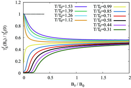
Figure 4: Magnetic field $B_{z}$ dependence of the $\gamma$-value from paraconductivity. The unit for the magnetic field is $B_{0}=m^{*}T_{0}/|e^{*}|$. The parameters are chosen as $a(T)=0.02(T-T_{0})$, $bm^{*}=0.005$, and $E_{\rm c}=4T_{0}$.

Figure 4 shows the exemplary results for the magnetic field dependence of $\gamma_{\rm S}(B_{z})=\sigma_{2}/\sigma_{1}^{2}B_{z}W$ which is normalized by the value at $B_{z}=0$. Above the mean-field transition temperature $T_{0}$, the $\gamma$-value decreases with increasing $B_{z}$, and it becomes nearly half at high fields. On the contrary, below $T_{0}$, the $\gamma$-value is small at low $B_{z}$ and increases by applying magnetic field. Although $\gamma_{\rm S}(B_{z})/\gamma_{\rm S}(0)$ goes to 1 at zero field, the corresponding $B_{z}$-range is so narrow that such regime (i.e. $a^{\prime}\gg\omega$) cannot be seen practically. This is because the value of $a^{\prime}$ for $T<T_{0}$ remains positive but is so tiny, and therefore the behavior is very sensitive to the small value of $B_{z}$. We note that in actual systems the component of normal conductivity is also finite and modifies the $\gamma$-value down to zero at high magnetic fields.

References

- (1) L. Onsager, Reciprocal Relations in Irreversible Processes. I. Phys. Rev. 37, 405 (1931).
- (2) R. Kubo, Statistical-Mechanical Theory of Irreversible Processes. I. General Theory and Simple Applications to Magnetic and Conduction Problems. J. Phys. Soc. Jpn. 12, 570 (1957).
- (3) G. L. J. A. Rikken, J. Fölling, P. Wyder, Electrical magnetochiral anisotropy. Phys. Rev. Lett. 87, 236602 (2001).
- (4) T. Morimoto, N. Nagaosa, Chiral anomaly and giant magnetochiral anisotropy in noncentrosymmetric Weyl semimetals. Phys. Rev. Lett. 117, 146603 (2016).
- (5) G. L. J. A. Rikken, E. Raupach, Observation of magneto-chiral dichroism. Nature 390, 493 (1997).
- (6) V. Krstić, S. Roth, M. Burghard, K. Kern, G. L. J. A. Rikken, Magneto-chiral anisotropy in charge transport through single-walled carbon nanotubes. J. Chem. Phys. 117, 11315 (2002).
- (7) G. L. J. A. Rikken, P. Wyder, Magnetoelectric anisotropy in diffusive transport. Phys. Rev. Lett. 94, 016601 (2005).
- (8) F. Pop, P. Auban-Senzier, E. Canadell, G. L. J. A. Rikken, N. Avarvari, Electrical magnetochiral anisotropy in a bulk chiral molecular conductor. Nat. Commun. 5, 3757 (2014).
- (9) T. Ideue et al., Bulk rectification effect in a polar semiconductor. Nat. Phys. 13, 578 (2017).
- (10) Nonreciprocal charge transport in noncentrosymmetric superconductors. R. Wakatsuki et al., Sci. Adv. 3, e1602390 (2017).
- (11) B.I. Halperin and D.R. Nelson, Resistive Transition in Superconducting Films. J. Low Temp. Phys. 36, 599 (1979).
- (12) Fluctuations near superconducting phase transitions. W. J. Skocpol and M. Tinkham, Rep. Prog. Phys. 38, 1049 (1975).
- (13) A. I. Larkin and A. A. Varlamov, Fluctuation Phenomena in Superconductors (Springer Berlin Heidelberg, Berlin, Heidelberg, 2008), pp. 369–458.
- (14) L. G. Aslamazov and A. I. Larkin, Effect of Fluctuations on the Properties of a Superconductor Above the Critical Temperature. Sov. Phys. Solid State 10, 875 (1968).
- (15) K. Maki, Critical Fluctuation of the Order Parameter in a Superconductor. I. Prog. Theor. Phys. 40, 193 (1968).
- (16) R. S. Thompson, Microwave, Flux Flow, and Flucutuation Resistance of Dirty Type-II Superconductors. Phys. Rev. B 1, 327 (1970).
- (17) A. Schmid, Diamagnetic Susceptibility at the Transition to the Superconducting State. Phys. Rev. 180, 527 (1969).
- (18) R. Wakatsuki and N. Nagaosa, Nonreciprocal current in noncentrosymmetric Rashba superconductors. arXiv:1712.02086 (2017).
- (19) S.-K. Yip, Fluctuations in an impure unconventional superconductor. Phys. Rev. B 41, 2612 (1990).
- (20) E. Bauer and M. Sigrist, editors, Non-Centrosymmetric Superconductors (Springer-Verlag Berlin Heidelberg, 2012).
- (21) S. Yip, Noncentrosymmetric superconductors. Annu. Rev. Condens. Matter Phys. 5, 15 (2014).
- (22) L. Fu, Hexagonal Warping Effects in the Surface States of the Topological Insulator Bi2Te3. Phys. Rev. Lett. 103, 266801 (2009).
- (23) D.R. Nelson and J.M. Kosterlitz, Universal Jump in the Superfluid Density of Two-Dimensional Superfluids. Phys. Rev. Lett. 39, 1201 (1977).
- (24) J.M. Kosterlitz, The critical properties of the two-dimensional model. J. Phys. C 7, 1046 (1974).
- (25) M. Tinkham, Introduction to Superconductivity (McGraw-Hill, New York, 1996).
- (26) J. Bardeen and M.J. Stephen, Theory o the Motion of Vortices in Superconductors. Phys. Rev. 140, A1197 (1965).
- (27) P. Nozières and W.F. Vinen, The Motion of Flux Lines in Type II Superconductors. Philos. Mag. 14, 667 (1966)
- (28) A. Schmid, A Time Dependent Ginzburg-Landau Eequation and its Application to the Problem of Resistivity in the Mixed State. Phys. kondens. Materie 5, 302 (1966).
- (29) N.B. Kopnin, Theory of Nonequilibrium Superconductivity. (Oxford University Press, Oxford, 2001).
- (30) J. Pearl, Current distribution in superconducting films carrying quantized fluxoids. Appl. Phys. Lett. 5, 65 (1964).
- (31) Y. Kato and C.-K. Chung, Nature of Driving Force on an Isolated Moving Vortex in Dirty Superconductors. J. Phys. Soc. Jpn. 85, 033703 (2016).
- (32) C.-S. Lee, B. Jankó, I. Derény, and A.-L. Barabási, Reducing vortex density in superconductors using the ‘ratchet’ effect. Nature 400, 337 (1999).
- (33) J.E. Villegas, S. Savel’ev, F. Nori, E.M. Gonzalez, J.V. Anguita, R. García, and J.L. Vicent, A Superconducting Reversible Rectifier That Controls the Motion of Magnetic Flux Quanta. Science 302, 1188 (2003).
- (34) J.E. Villegas, E.M. Gonzalez, M.P. Gonzalez, J.V. Anguita, and J.L. Vicent, Experimental ratchet effect in superconducting films with periodic arrays of asymmetric potentials. Phys. Rev. B 71, 024519 (2005).
- (35) Y. Saito et al., private communication.
- (36) P. Reimann, C. Van den Broeck, H. Linke, P. Hänggi, J.M. Rubi, and A. Pérez-Madrid, Giant Acceleration of Free Diffusion by Use of Tilted Periodic Potentials. Phis. Rev. Lett. 87, 010602, (2001).
- (37) N. Reyren, S. Thiel, A. D. Caviglia, L. F. Kourkoutis, G. Hammerl, C. Richter, C. W. Schneider, T. Kopp, A.-S. Rüetschi, D. Jaccard, M. Gabay, D. A. Muller, J.-M. Triscone, and J. Mannhart, Superconducting Interfaces Between Insulating Oxides. Science 317, 1196 (2007).
- (38) A. D. Caviglia, S. Gariglio, N. Reyren, D. Jaccard, T. Schneider, M. Gabay, S. Thiel, G. Hammerl, J. Mannhart, and J.-M. Triscone, Electric field control of the LaAlO3/SrTiO3 interface ground state. Nature 456, 624 (2008).
- (39) G. Herranz, G. Singh, N. Bergeal, A. Jouan, J. Lesueur, J. Gázquez, M. Varela, M. Scigaj, N. Dix, F. Sánchez, and J. Fontcuberta, Engineering two-dimensional superconductivity and Rashba spin-orbit coupling in LaAlO3/SrTiO3 quantum wells by selective orbital occupancy. Nat. Commun. 6, 6028 (2015).
- (40) E. Maniv, M. B. Shalom, A. Ron, M. Mograbi, A. Palevski, M. Goldstein, and Y. Dagan, Strong correlations elucidate the electronic structure and phase diagram of LaAlO3/SrTiO3 interface. Nat. Commun. 6, 8239 (2015).
- (41) K. W. Kim, T. Morimoto, and N. Nagaosa, Shift charge and spin photocurrents in Dirac surface states of topological insulator. Phys. Rev. B, 95, 035134 (2017).
- (42) Y. Saito et. al., Superconductivity protected by spin-valley locking in ion-gated MoS2. Nat. Phys. 12, 144 (2016).
- (43) Y.B. Kim and M.J. Stephen, in Superconductivity, ed. R.D. Parks (Marcel Dekker, New York, 1969).
- (44) E. Abrahams, R.E. Prange, and M.J. Stephen, Effect of a mangetic field on fluctuations above Tc. Physica 55, 230 (1971).
- (45) see for example, P.M. Chaikin and T.C. Lubensky. Principles of Condensed Matter Physics (Cambridge University Press, New York, 1995).