Firing rate and spatial correlation in a stochastic neural field model

Abstract.

This paper studies a stochastic neural field model that is extended from our previous paper [14]. The neural field model consists of many heterogeneous local populations of neurons. Rigorous results on the stochastic stability are proved, which further imply the well-definedness of quantities including mean firing rate and spike count correlation. Then we devote to address two main topics: the comparison with mean-field approximations and the spatial correlation of spike count. We showed that partial synchronization of spiking activities is a main cause for discrepancies of mean-field approximations. Furthermore, the spike count correlation between local populations are studied. We find that the spike count correlation decays quickly with the distance between corresponding local populations. Some mathematical justifications of the mechanism of this phenomenon is also provided.

1. Introduction

In mathematical neuroscience, numerous neuronal models have been proposed and studied. Many models such as the Hodgkin-Huxley model aim to accurately describe the realistic biophysics process. When more anatomical and physiological details, such as ionic channels, dendritic tree, spatial structure of axon, and synapse, are involved, the model usually becomes too complex to study, especially when applying to a large-scale network. On the other end of the spectrum, there are many mean field models such as Wilson-Cowan model [20, 21] and various population density models [9, 5, 4] that model the behavior of a neural population by a few coarse-grained variables. It is easier to use a mean-field model to describe the neuronal activities in a large area of the cortex. However, mean field models usually assume that neuronal interactions are weak, which cause some inevitable discrepancies.

Consider a large area of the cortex, such as several hundreds of hypercolumns in the primary visual cortex. In order to study experimentally observed phenomena such as surround suppression, neuronal models at this scale are necessary. Needless to say, it is not realistic to model each of millions of neurons by detailed models like the Hodgkin-Huxley model. Some coarse graining is necessary for these large scale problems. On the other hand, it is usually not clear how much information a mean field model could preserve. The mechanism of such discrepancy is also little studied. In our previous paper [14], these questions are partially answered for a stochastic neuron model that models a homogeneous and densely connected neuronal population. Several mean field approximations of the stochastic model studied in [14] are exactly solvable. We showed that the strong excitation-inhibition interplay during the partially synchronous spike volley, called a multiple firing event, contributes significantly to the discrepancy of the mean-field approximation. It is believed that such multiple firing event is related to the Gamma rhythm in the cortex.

The aim of this paper is two-fold. The first half of this paper serves as an extension to our previous paper [14]. We generalize the stochastic model studied in [14] to a neural field model that describes the neuronal activities of neurons in a large and heterogeneous domain. More precisely, we consider the coupling of finitely many local neuron populations, each of which is described by a stochastic model studied in [14]. This extension is necessary because the real cerebral cortex consists of numerous relatively homogeneous local structures, while the neuronal activities in different local structures can be very different. Take the visual cortex as an example again. Responses to stimulus orientation are very different in orientation columns with different orientation preferences, even if they are spatially close to each other [12, 11]. Similar as in [14], we proved the stochastic stability of the Markov process generated by the model, which implies that many quantities like the mean firing rate are well-defined. Then we proposed two exactly solvable mean-field approximations of our neural field model. The discrepancy of the mean-field approximations is analyzed. Same as in the homogeneous population model, the discrepancy of a mean field model is mainly caused by the emergent coordinated neuronal activities, and is significantly exacerbated when the neuron spikes become synchronized.

A more important result presented in this paper is the spatial correlation of spike counts in the neural field. This is not studied in our previous paper [14]. We found that the multiple firing event in nearest-neighbor local populations are highly correlated. However, this correlation decays quickly with increasing distance between two local populations. This is consistent with the experimental observations that the Gamma rhythm is very local [7, 13, 15]. Two analytical studies are carried out to investigate this spatial correlation. We first propose an ODE model that describe the activity during a multiple firing event. This ODE model shows that the strong excitatory and inhibitory current during a multiple firing event at one local population is very likely to induce a similar multiple firing event in its neighbor local populations. This explains the mechanism of the spatial correlation. Then we studied the possible mechanism of the spatial correlation decay. One salient feature of the multiple firing event is its diversity. When starting from the same profile, the spike count of a multiple firing event can have very high volatility, measured by the coefficient of variation. The volatility significantly decreases when the multiple firing event is close to a synchronous spiking event. We believe this diversity at least partially contributes to the quick decay of the spatial correlation. This is verified by our numerical simulation result, in which the most synchronous network has the slowest decay of the spatial correlation.

The organization of this paper is as follows. Section 1 is the introduction. We provide the mathematical description of the neural field model in Section 2. Section 3 is devoted to the proof of the stochastic stability and several useful corollaries. Then we provide five network examples with distinct features in Section 4 for later investigations. Two mean-field approximations are presented in Section 5. We also analyze their discrepancies in the same section. Section 6 is devoted to the spatial correlation. We demonstrate both phenomena and mechanism of the spatial correlation between spike counts of different local populations. Section 7 is the conclusion.

2. Stochastic model of many interacting neural populations

We consider a stochastic model that describes the interaction of many local populations in the cerebral cortex. Each local population consists of hundreds of interacting excitatory and inhibitory neuron. The setting of this model is quit generic, but it aims to describe some of the spiking activities of realistic brain parts. In particular, one can treat a local population as an orientation column in the primary visual cortex. We will only prescribe the rules of external inputs and interactions between neurons. All spatial and temporal correlated spiking activities in this model are emergent from interactions of neurons.

2.1. Model description.

We consider an $M\times N$ array of local populations of neurons, each of which are homogeneous and densely connected by local circuitries. In addition, neurons in nearest neighbor of local populations are connected. Each local population consists of $N_{E}$ excitatory neurons and $N_{I}$ inhibitory neurons. Similar to the treatment in [14], we have the following assumptions in order to describe the activity of this population by a Markov process.

• The membrane potential of each neuron can only take finitely many discrete values.

• The external current to each neuron is in the form of independent Poisson processes. The rate of Poisson kicks to all neurons of the same type in each local population is a constant.

• A neuron spikes when its membrane potential reaches a given threshold. After a spike, a neuron stays at a refractory state for an exponentially distributed amount of time.

• When an excitatory (resp. inhibitory) spike occurs at a local population, a set of postsynaptic neurons from this local population and its nearest neighbor local populations are randomly chosen. After an exponenitally distributed random time, the membrane potential of each chosen postsynaptic neuron goes up (resp. down).

More precisely, we consider $M\times N$ local populations $\{L_{m,n}\}$ with $m=1,\cdots,M$ and $n=1,\cdots,N$. $L_{m,n}$ and $L_{m^{\prime},n^{\prime}}$ are considered to be nearest neighbors if and only if $m=n^{\prime}$, $|n-n^{\prime}|=1$ or $|m-m^{\prime}|=1$, $n=n^{\prime}$. For each $(m,n)$, denote the set of indices of its nearest neighbors local populations by $\mathcal{N}(m,n)$. Each population $L_{m,n}$ consists of $N_{E}$ excitatory neurons, labeled

$$(m,n,1),(m,n,2),\cdots,(m,n,N_{E})$$

and $N_{I}$ inhibitory neurons, labeled

$$(m,n,N_{E}+1),(m,n,N_{E}+2),\cdots,(m,n,N_{E}+N_{I})\,.$$

In other words, each neuron has a unique label $(m,n,k)$. The membrane potential of neuron $(m,n,k)$, denoted $V_{(m,n,k)}$, takes value in a finite set

$$\Gamma:=\{-M_{r},-M_{r}+1,\cdots,-1,0,1,2,\cdots,M\}\cup\{\mathcal{R}\}\,,$$

where $M$ and $M_{r}$ are two integers for the threshold potential and the inhibitory reversal potential, respectively. When $V_{(m,n,k)}$ reaches $M$, the neuron fires a spike and reset its membrane potential to $\mathcal{R}$. After an exponentially distributed amount of time with mean $\tau_{R}$, $V_{(m,n,k)}$ leaves $\mathcal{R}$ and jumps to $0$.

We first describe the external current that models the input from other parts of the brain or the sensory input. As in [14], the external current received by a neuron is modeled by a homogeneous Poisson process. The rate of this Poisson process is identical for the same type of neurons in the same local population. Neurons in different local population receive different external current, which makes this model spatially heterogeneous. More precisely, we assume the rate of such Poisson kick of an excitatory (resp. inhibitory) neuron in local population $L_{m,n}$ to be $\lambda_{m,n}^{E}$ (resp. $\lambda_{m,n}^{I}$). When a kick is received by neuron $(m,n,k)$ and it is not at state $\mathcal{R}$, $V_{(m,n,k)}$ jumps up by $1$ immediately. If it reaches $M$, a spike is fired. Neurons at state $\mathcal{R}$ do not respond to external kicks.

The rule of interactions among neurons is the following. We assume that a postsynaptic kick from an E (resp. I) neuron takes effect after an exponentially distributed amount of time with mean $\tau_{E}$ (resp. $\tau_{I}$). To model this delay effect, we describe the state of neuron $(m,n,k)$ by a triplet $(V_{(m,n,k)},H^{E}_{(m,n,k)},H^{I}_{(m,n,k)})$, where $H^{E}_{(m,n,k)}$ (resp. $H^{I}_{(m,n,k)}$) denote the number of received E (resp. I) postsynaptic kicks that has not yet taken effect. Further, we assume that the delay of postsynaptic kicks are independent. Therefore, two exponential clocks corresponding to excitatory and inhibitory kicks are associated to each neuron, with rates $H^{E}_{(m,n,k)}\tau_{E}^{-1}$ and $H^{I}_{(m,n,k)}\tau_{I}^{-1}$ respectively. When the clock corresponding to excitatory (resp. inhibitory) kicks rings, an excitatory (resp. inhibitory) kick takes effect according to the rules described in the following paragraph.

Let $Q,Q^{\prime}\in\{E,I\}$. When a postsynaptic kick from a neuron of type $Q$ takes effect at a neuron of type $Q^{\prime}$ after the delay time as described above, the membrane potential of the postsynaptic neuron, say neuron $(m,n,k)$, jumps instantaneously by a constant $S_{Q^{\prime},Q}$ if $V_{(m,n,k)}\neq\mathcal{R}$. No change happens if $V_{(m,n,k)}=\mathcal{R}$. If after the jump we have $V_{(m,n,k)}\geq M$, neuron $(m,n,k)$ fires a spike and jumps to state $\mathcal{R}$. Same as in [14], if constant $S_{Q^{\prime},Q}$ is not an integer, we let $u$ be a Bernoulli random variable with $\mathbb{P}[u=1]=S_{Q^{\prime},Q}-\left\lfloor S_{Q^{\prime},Q}\right\rfloor$ that is independent of all other random variables in the model. Then the magnitude of the postsynaptic jump is set to be the random number $\left\lfloor S_{Q^{\prime},Q}\right\rfloor+u$.

It remains to describe the connectivity within and between local populations. We assume that each local population is densely connected and homogeneous, while different local populations are heterogeneous in a way that the external currents are different. For example, each local population can be thought as an orientation column in the primary visual cortex. Hence nearest-neighbor populations receive very different external drives due to their different orientational preferences. Same as in [14], the connectivity in our model is random and time-dependent. For $Q,Q^{\prime}\in\{E,I\}$, we choose two parameters $P_{Q,Q^{\prime}},\rho_{Q,Q^{\prime}}\in[0,1]$ representing the local and external connectivity respectively. When a neuron of type $Q^{\prime}$ in a local population $L_{m,n}$ fires a spike, every neuron of type $Q$ in the local population $L_{m,n}$ is postsynaptic with probability $P_{Q,Q^{\prime}}$, while every neuron of type $Q$ in the nearest-neighbor populations $L_{m^{\prime},n^{\prime}}$ receives this postsynaptic kick with probability $\rho_{Q,Q^{\prime}}$. In other words, neurons of the same type in the same local population are assumed to be indistinguishable.

2.2. Common parameters for simulations.

Although our theoretical results are valid for all parameters, in numerical simulations we will stick to the following set of parameters in order to be consistent with [14]. Throughout this paper, we assume that $N_{E}=300$, $N_{I}=100$ for the size of local populations, $M=100$, $M_{r}=66$ for the thresholds, $P_{EE}=0.15$, $P_{IE}=P_{EI}=0.5$ and $P_{II}=0.4$ for local conductivities. The conductivities to nearest neighbors are assumed to be proportional to the corresponding local conductivities. We set two parameters $\mbox{ratio}_{E}$ and $\mbox{ratio}_{I}$ and let $\rho_{QE}=\mbox{ratio}_{E}P_{QE}$, $\rho_{QI}=\mbox{ratio}_{I}P_{QI}$ for $Q=I,E$. Further, we assume that $\mbox{ratio}_{I}=0.6\mbox{ratio}_{E}$ as inhibitory neurons are known to be more “local”. The strengths of postsynaptic kicks are assumed to be $S_{EE}=5$, $S_{IE}=2$, $S_{EI}=3$, and $S_{II}=3.5$. The length of refractory period is set as $\tau_{\mathcal{R}}=4\mbox{ms}$. Since AMPA synapses act faster than GABA synapses, in general $\tau_{E}$ is assumed to be faster than $\tau_{I}$. Values of $\tau_{E}$ and $\tau_{I}$ are two changing parameters that are used to control the degree of synchrony of the network. External drive rates $\lambda_{m,n}^{E}$ and $\lambda_{m,n}^{I}$ are determined when describing examples with different spatial structures.

3. Stochastic stability and proofs

The aim of this section is to show the stochastic stability of the model presented in Section 2. As a corollary, we have well-defined and computable local and global firing rates, and the spike count correlation between local populations.

3.1. Statement of results.

The neural field model described above generates a Markov jump process $\Phi_{t}$ on a countable state space

$$\mathbf{X}=(\Gamma\times\mathbb{Z}_{+}\times\mathbb{Z}_{+})^{M\times N\times(N_{E}+N_{I})}\,.$$

The state of neuron $(m,n,k)$ is given by the triplet $(V_{(m,n,k)},H^{E}_{(m,n,k)},H^{I}_{(m,n,k)})$, where $V_{(m,n,k)}\in\Gamma$ and $H^{E}_{i},H^{I}_{i}\in\mathbb{Z}_{+}:=\{0,1,2,\cdots\}$. The transition probabilities of $\Phi_{t}$ are denoted by $P^{t}(\mathbf{x},\mathbf{y})$, i.e.,

$$P^{t}(\mathbf{x},\mathbf{y})=\mathbb{P}[\Phi_{t}=\mathbf{y}\,|\,\Phi_{0}=\mathbf{x}]\,.$$

If $\mu$ is a probability distribution on $\mathbf{X}$, the left operator of $P^{t}$ acting on $\mu$ is

$$\mu P^{t}(\mathbf{x})=\sum_{\mathbf{y}\in\mathbf{X}}\mu(\mathbf{y})P^{t}(\mathbf{y},\mathbf{x})\,.$$

Similarly, the right operator of $P^{t}$ acting on a real-valued function $\eta:\mathbf{X}\rightarrow\mathbb{R}$ is

$$P^{t}\eta(\mathbf{x})=\sum_{\mathbf{y}\in\mathbf{X}}P^{t}(\mathbf{x},\mathbf{y})\eta(\mathbf{y})\,.$$

Finally, for any probability measure $\mu$ and real-valued function $\eta$ on $\mathbf{X}$, we take the convention that

$$\mu(\eta)=\sum_{\mathbf{x}\in\mathbf{X}}\eta(\mathbf{x})\mu(\mathbf{x})\,.$$

For the stochastic stability, we mean the existence, uniqueness, and ergodicity of the invariant measure for $\Phi_{t}$. Note that $\mathbf{X}$ has countably infinite states. Hence Markov chains on $\mathbf{X}$ need not admit an invariant probability measure.

Define the total number of pending excitatory (resp. inhibitory) kicks at a state $\mathbf{x}\in\mathbf{X}$ as

$$H^{E}(\mathbf{x})=\sum_{m=1}^{M}\sum_{n=1}^{N}\sum_{k=1}^{N_{E}+N_{I}}H^{E}_{(m,n,k)}$$

and

$$H^{I}(\mathbf{x})=\sum_{m=1}^{M}\sum_{n=1}^{N}\sum_{k=1}^{N_{E}+N_{I}}H^{I}_{(m,n,k)}\,.$$

Further we let $U(\mathbf{x})=H^{E}(\mathbf{x})+H^{I}(\mathbf{x})+1$. For any signed measure on the Borel $\sigma$-algebra of $\mathbf{X}$, denoted by $\mathcal{B}(X)$, we define the $U$-weighted total variation norm to be

$$\|\mu\|_{U}=\sum_{\mathbf{x}\in\mathbf{X}}U(\mathbf{x})|\mu(\mathbf{x})|\,,$$

and let

$$L_{U}(\mathbf{X})=\{\mu\mbox{ on }\mathbf{X}\,|\,\|\mu\|_{U}<\infty\}\,.$$

In addition, for any measurable function $\eta(\mathbf{x})$ on $\mathbf{X}$, we let

$$\sup_{\mathbf{x}\in\mathbf{X}}\frac{|\eta(\mathbf{x})|}{U(\mathbf{x})}$$

be the $U$-weighted supreme norm.

Theorem 3.1.

$\Phi_{t}$ admits a unique invariant probability measure $\pi\in L_{U}(\mathbf{X})$. In addition, there exist constants $C_{1}$, $C_{2}>0$ and $r\in(0,1)$ such that

• (a) for any initial distribution $\mu\in L_{U}(\mathbf{X})$,

  $$\|\mu P^{t}-\pi\|_{U}\leq C_{1}r^{t}\|\mu-\pi\|_{U}\,;$$

• (b) for any measurable function $\eta$ with $\|\eta\|_{U}<\infty$,

  $$\|P^{t}\eta-\pi(\eta)\|_{U}\leq C_{2}r^{t}\|\eta-\pi(\eta)\|_{U}\,.$$

Theorem 3.1 guarantees that the local/global firing rate and the spike count correlation between local populations are well defined. Let $L_{m,n}$ be a given local population. For $Q\in\{E,I\}$, let $N^{Q}_{(m,n)}([a,b])$ be the number of neuron spikes fired by type $Q$ neurons in $L_{m,n}$ on the time interval $[a,b]$. As discussed in [14], the mean firing rate of the local population $(m,n)$ is defined to be

$$F^{Q}_{m,n}=\frac{1}{T}\mathbb{E}_{\pi}[N^{Q}_{(m,n)}([0,T])]\,,$$

where $\mathbb{E}_{\pi}$ is the expectation with respect to the invariant probability measure $\pi$. This definition is independent of $T$ by the invariance of $\pi$.

Let $T$ be a fixed time window, we can further define the covariance of spike count between $Q_{1}$-population in $L_{m,n}$ and $Q_{2}$-population in $L_{m^{\prime},n^{\prime}}$ as

$$\mbox{cov}_{T}^{Q_{1},Q_{2}}(m,n;m^{\prime},n^{\prime})=\mathbb{E}_{\pi}[N^{Q_{1}}_{(m,n)}([0,T])N^{Q_{2}}_{(m^{\prime},n^{\prime})}([0,T])]-T^{2}N_{Q_{1}}N_{Q_{2}}F^{Q_{1}}_{m,n}F^{Q_{2}}_{m^{\prime},n^{\prime}}\,.$$

The Pearson correlation coefficient of spike count can be defined similarly. For $Q_{1}$-population in $L_{m,n}$ and $Q_{2}$-population in $L_{m^{\prime},n^{\prime}}$, we have

$$\rho^{Q_{1},Q_{2}}_{T}(m,n,m^{\prime},n^{\prime})=\frac{\mbox{cov}_{T}^{Q_{1},Q_{2}}(m,n,m^{\prime},n^{\prime})}{\sigma^{Q_{1}}_{T}(m,n)\cancel{\sigma^{Q_{2}}_{T}(m,n)}\sigma^{Q_{2}}_{T}(m^{\prime},n^{\prime})}\,,$$

where

$$\sigma^{Q}_{T}(m,n)=\sqrt{\mbox{var}_{\pi}(N^{Q}_{(m,n)}([0,T]))}$$

for $Q\in\{E,I\}$.

One can also consider the correlation of the total spike count between two local populations. Let $N_{(m,n)}([0,T])$ be the number of excitatory and inhibitory spikes produced by $L_{m,n}$ on $[0,T]$ when starting from the steady state. Then the correlation $\mbox{cov}_{T}(m,n,m^{\prime},n^{\prime})$ and the Pearson correlation coefficient $\rho_{T}(m,n,m^{\prime},n^{\prime})$ can be defined analogously.

The following corollaries implies that the mean firing rate and the spike count correlation are computable.

Corollary 3.2.

For $Q\in\{E,I\}$, $1\leq m\leq M$, and $1\leq n\leq N$, the local firing rate $F^{Q}_{m,n}<\infty$. In addition, for any initial value $\mathbf{x}\in X$,

$$\lim_{T\rightarrow\infty}\frac{N^{Q}_{(m,n)}([0,T])}{N_{Q}T}=F^{Q}_{(m,n)}$$

almost surely.

Corollary 3.3.

For $Q_{1},Q_{2}\in\{E,I\}$, $1\leq m,m^{\prime}\leq M$, and $1\leq n,n^{\prime}\leq N$, the covariance $\mbox{cov}_{T}^{Q_{1},Q_{2}}(m,n;m^{\prime},n^{\prime})<\infty$. In addition, for any initial value $\mathbf{x}\in X$,

$$\lim_{K\rightarrow\infty}\frac{1}{K}\sum_{k=0}^{K-1}N^{Q_{1}}_{(m,n)}([kT,(k+1)T))N^{Q_{2}}_{(m^{\prime},n^{\prime})}([kT,(k+1)T))=\mathbb{E}_{\pi}[N^{Q_{1}}_{(m,n)}([0,T])N^{Q_{2}}_{(m^{\prime},n^{\prime})}([0,T])]$$

almost surely. In other words $\mbox{cov}_{T}^{Q_{1},Q_{2}}(m,n;m^{\prime},n^{\prime})$ is computable.

Corollary 3.4.

For $1\leq m,m^{\prime}\leq M$, and $1\leq n,n^{\prime}\leq N$, the covariance $\mbox{cov}_{T}(m,n;m^{\prime},n^{\prime})<\infty$. In addition, for any initial value $\mathbf{x}\in X$,

$$\lim_{K\rightarrow\infty}\frac{1}{K}\sum_{k=0}^{K-1}N_{(m,n)}([kT,(k+1)T])N_{(m^{\prime},n^{\prime})}([kT,(k+1)T))=\mathbb{E}_{\pi}[N_{(m,n)}([0,T])N_{(m^{\prime},n^{\prime})}([0,T])]$$

almost surely. In other words $\mbox{cov}_{T}(m,n;m^{\prime},n^{\prime})$ is computable.

3.2. Probabilistic Preliminaries

Let $\Psi_{n}$ be a Markov chain on a countable state space $(X,\mathcal{B})$ with transition kernels $\mathcal{P}(x,\cdot)$. Let $W:X\rightarrow[1,\infty)$ be a real-valued function. The following general results on geometric ergodicity is well known.

Assume $\Psi_{n}$ satisfies the following conditions.

• There exist constants $K\geq 0$ and $\gamma\in(0,1)$ such that

  $$(\mathcal{P}W)(x)\leq\gamma W(x)+K$$

  for all $x\in X$.

• There exists a constant $\alpha\in(0,1)$ and a probability distribution $\nu$ on $\mathbf{X}$ so that

  $$\inf_{x\in C}\mathcal{P}(x,\cdot)\geq\alpha\nu(\cdot)\,,$$

  with $C=\{x\in X\,|\,W(x)\leq R\}$ for some $R>2K/(1-\gamma)$, where $K$ and $\gamma$ are from (a).

The following result was proved in [16] and [8] using different methods. Note that the original result in [16, 8] is for a generic measurable state space. The result applies to countable state space with the Borel $\sigma$-algebra (which is essentially the discrete $\sigma$-algebra).

Theorem 3.5.

Assume (a) and (b). Then $\Psi_{n}$ admits a unique invariant measure $\pi\in L_{W}(X)$. In addition, there exist constants $C,C^{\prime}>0$ and $r\in(0,1)$ such that (ii) for all $\mu,\nu\in L_{W}(X)$,

$$\|\mu\mathcal{P}^{n}-\nu\mathcal{P}^{n}\|_{W}\leq Cr^{n}\|\mu-\nu\|_{W}\,,$$

and (i) for all $\xi$ with $\|\xi\|_{W}<\infty$,

$$\|\mathcal{P}^{n}\xi-\pi(\xi)\|_{W}\leq C^{\prime}r^{n}\|\xi-\pi(\xi)\|_{W}\,.$$

We also need the following law of large numbers for martingale difference sequence to prove the corollary.

Theorem 3.6 (Theorem 3.3.1 of [19]).

Let $X_{n}$ be a martingale difference sequence with respect to $\mathcal{F}_{n}$. If

$$\sum_{n=1}^{\infty}\frac{\mathbb{E}[|X_{n}|^{2}]}{n^{2}}<\infty\,,$$

then

$$\frac{1}{N}\sum_{n=1}^{N}X_{n}\rightarrow 0\quad a.s.$$

3.3. Proof of main results.

For a step size $h>0$ that will be described later, we define the time-$h$ sample chain as $\Phi^{h}_{n}=\Phi_{nh}$. The superscript $h$ is dropped when it leads to no confusion. Recall that $U(\mathbf{x})=H^{E}(\mathbf{x})+H^{I}(\mathbf{x})+1$. The following two lemmas verify conditions (a) and (b) for Theorem 3.5.

Lemma 3.7.

For $h>0$ sufficiently small, there exist constants $K>0$ and $\gamma\in(0,1)$, such that

$$P^{h}U\leq\gamma U+K\,.$$

This proof is similar to that of Lemma 2.4 of [14]. We include it for the sake of completeness of this paper.

Proof.

During $(0,h]$, let $N_{out}$ be the number of pending kicks from $H^{E}(\mathbf{x})$ and $H^{I}(\mathbf{x})$ that takes effect and $N_{in}$ be the number of new spikes produced. We have

$$P^{h}U(\mathbf{x})=\mathbb{E}_{\mathbf{x}}[U(\Phi_{h})]=U(\mathbf{x})-\mathbb{E}_{\mathbf{x}}[N_{out}]+\mathbb{E}_{\mathbf{x}}[N_{in}]\,.$$

The probability that an excitatory (resp. inhibitory) pending kick takes effect on $(0,h]$ is $(1-e^{-h/\tau^{E}})$ (resp. $(1-e^{-h/\tau^{I}})$). Hence for $h$ sufficiently small, we have

$$\mathbb{E}_{\mathbf{x}}[N_{out}]\geq(H^{E}(\mathbf{x})+H^{I}(\mathbf{x}))(1-e^{-h/\max\{\tau^{E},\tau^{I}\}})\geq\frac{1}{2\max\{\tau^{E},\tau^{I}\}}\ h\ (U(\mathbf{x})-1)\,.$$

For a neuron $(m,n,k)$, after each spike it spends an exponential time with mean $\tau_{\mathcal{R}}$ at state $\mathcal{R}$. Hence the number of spikes produced by neuron $(m,n,k)$ is at most

$$1+\mathbb{E}[\mbox{Pois}(h/\tau_{\mathcal{R}})]=1+h/\tau_{\mathcal{R}}\,,$$

where $\mbox{Pois}(\lambda)$ is a Poisson random variable with rate $\lambda$. Hence

$$\mathbb{E}_{\mathbf{x}}[N_{in}]\leq MN(N_{E}+N_{I})\cdot(1+h/\tau_{\mathcal{R}})\,.$$

The proof is completed by letting

$$\gamma=1-h/(2\max\{\tau^{E},\tau^{I}\})\qquad\mbox{and}\qquad K=MN(N_{E}+N_{I})\cdot(1+h/\tau_{\mathcal{R}})\ +\frac{h}{2\max\{\tau^{E},\tau^{I}\}}.$$

∎

For $b\in\mathbb{Z}_{+}$, let

$$C_{b}=\{\mathbf{x}\in\mathbf{X}|H^{E}(\mathbf{x})+H^{I}(\mathbf{x})\leq b\}\,.$$

Lemma 3.8.

Let $\mathbf{x}_{0}$ be the state that $H^{E}=H^{I}=0$ and $V_{(m,n,k)}=\mathcal{R}$ for all $1\leq m\leq M$, $1\leq n\leq N$, and $1\leq k\leq N_{E}+N_{I}$. Then for any $h>0$, there exists a constant $\delta=\delta(b,h)$ depending on $b$ such that there exists a constant $c$ depending on $b$ and $h$ such that,

$$P^{h}(\mathbf{x},\mathbf{x}_{0})>c\quad\mbox{ for all }\mathbf{x}\in C_{b}$$

Proof.

For each $\mathbf{x}\in C_{b}$, it is sufficient to construct an event that moves from $\mathbf{x}$ to $\mathbf{x}_{0}$ with a uniform positive probability. Below is one of many possible constructions.

• On $(0,h/2]$, a sequence of external Poisson kicks drives each $V_{(m,n,k)}$ to the threshold value $M$, hence puts $V_{(m,n,k)}=\mathcal{R}$. Once at $\mathcal{R}$, $V_{(m,n,k)}$ remains there before $t=h$. In addition, no pending kicks takes effect on $(0,h/2]$.

• All pending kicks at state $\mathbf{x}$ take effect on $(h/2,h]$. Obviously this has no effect on membrane potentials.

Since $b$ is bounded, the number of pending kicks is less than $b+MN(N_{E}+N_{I})<\infty$. It is easy to see that this event happens with positive probability. ∎

Lemmas 3.7 and 3.8 together imply Theorem 3.1.

Proof of Theorem 3.1.

Choose step size $h$ as in Lemma 3.7. By Lemmata 3.7, 3.8 and Theorem 3.5, $\Phi^{h}$ admits a unique invariant probability measure $\pi_{h}$ in $L_{U}(\mathbf{X})$.

We then show that $\pi_{h}$ is invariant under $\Phi_{t}$ for any $t>0$. This can be done by proving the following “continuity at zero” condition, which means for any probability measure $\mu$ on $\mathbf{X}$,

$$\lim_{t\rightarrow 0}\|\mu P^{t}-\mu\|_{TV}=0\,.$$

For any small $\epsilon>0$, there exists $b<\infty$ and (small) $\delta>0$ such that if $U=\{\mathbf{x}\in\mathbf{X}\,|\,H^{E}(\mathbf{x})+H^{I}(\mathbf{x})<b\}$, then (i) $\mu(U)>1-\epsilon/4$ and (ii) $\mathbb{P}[\mbox{ no clock rings on }[0,\delta)]\geq 1-\epsilon/4$. For any set $A\subset\mathbf{X}$, we have

$$(\mu P^{\delta})(A) = \sum_{\mathbf{x}\in\mathbf{X}}P^{\delta}(\mathbf{x},A)\mu(\mathbf{x})$$

$$= \sum_{\mathbf{x}\in U\cap A}P^{\delta}(\mathbf{x},A)\mu(\mathbf{x})+\sum_{\mathbf{x}\in U-A}P^{\delta}(\mathbf{x},A)\mu(\mathbf{x})+\sum_{\mathbf{x}\in U_{c}}P^{\delta}(\mathbf{x},A)\mu(\mathbf{x})$$

$$= \mu(U\cap A)-a_{1}+a_{2}+a_{3}\,,$$

where

$$a_{1} = \sum_{\mathbf{x}\in U\cap A}(1-P^{\delta}(\mathbf{x},A))\mu(\mathbf{x})\leq\frac{\epsilon}{4}\mu(U\cap A)\leq\frac{\epsilon}{4}$$

$$a_{2} = \sum_{\mathbf{x}\in U\setminus A}P^{\delta}(\mathbf{x},A)\mu(\mathbf{x})\leq\frac{\epsilon}{4}\mu(U\setminus A)\leq\frac{\epsilon}{4}$$

$$a_{3} = \sum_{\mathbf{x}\in U^{c}}P^{\delta}(\mathbf{x},A)\mu(\mathbf{x})\leq\mu(U^{c})\leq\frac{\epsilon}{4}\,.$$

Further, $\mu(A)-\mu(U\cap A)\leq\mu(U^{c})<\frac{\epsilon}{4}$. Hence

$$\epsilon>\sup_{A\subset\mathbf{X}}|(\mu P^{\delta})(A)-\mu(A)|\geq\|\mu P^{\delta}-\mu\|_{TV}\,.$$

This implies the “continuity at zero” condition.

Notice that $\pi_{h}$ is invariant for any $\Psi^{hj/k}_{n}$, where $j,k\in\mathbb{Z}^{+}$ (Theorem 10.4.5 of [16]). Assume $t/h\notin\mathbb{Q}$ without loss of generality. By the density of orbits in irrational rotations, there exists sequences $a_{n}$, $b_{n}\in\mathbb{Z}^{+}$ such that

$$d_{n}:=t-\frac{a_{n}}{b_{n}}h\searrow 0\,.$$

Therefore,

$$\|\pi_{h}P^{t}-\pi_{h}\|_{TV}=\lim_{n\rightarrow\infty}\|\pi_{h}P^{\frac{a_{n}}{b_{n}}h}P^{d_{n}}-\pi_{h}\|=\lim_{n\rightarrow\infty}\|\pi_{h}P^{d_{n}}-\pi_{h}\|_{TV}=0$$

by the “continuity at zero” condition. Hence $\pi_{h}$ is invariant with respect to $P^{t}$.

It remains to prove the exponential convergence for any $t>0$. By Lemma 3.7, there exists $B=K+1<\infty$ such that $P^{t}U\leq BU$ for all $t<h$. Let $n=\left\lfloor t/h\right\rfloor$ and $d=t-hn$. We have

$$\|\mu P^{t}-\nu P^{t}\|_{U} = \|(\mu P^{d})P^{nh}-(\nu P^{d})P^{nh}\|_{U}$$

$$= Cr^{n}\cdot\|\mu P^{d}-\nu P^{d}\|_{U}\ \leq\ BCr^{n}\|\mu-\nu\|_{U}$$

and

$$\|P^{t}\xi-\pi(\xi)\|_{U} = \|P^{nh}(P^{d}\xi)-P^{nh}(P^{d}\pi(\xi))\|_{U}$$

$$= Cr^{n}\cdot\|P^{d}\xi-P^{d}\pi(\xi)\|_{U}\ \leq\ BCr^{n}\|\xi-\pi(\xi)\|_{U}\,.$$

This completes the proof. ∎

Proof of Corollary 3.2.

By the invariance of $\pi$, for any local population $L_{m,n}$ and any $Q\in\{E,I\}$, we have

$$F^{Q}_{m,n}=\mathbb{E}_{\pi}[N^{Q}_{(m,n)}([0,1])]\,.$$

For every $\mathbf{x}\in\mathbf{X}$ we have

$$\mathbb{E}_{\mathbf{x}}[N^{Q}_{m,n}([0,1])]\leq N_{Q}(1+\mathbb{E}[\mbox{ Pois}(1/\tau_{\mathcal{R}})])=N_{Q}(1+1/\tau_{\mathcal{R}})\,.$$

Thus $F^{Q}_{m,n}=\mathbb{E}_{\pi}[N^{Q}_{(m,n)}([0,1])]<\infty$.

It remains to prove the law of large number. Without loss of generality let $Q=E$. Let

$$\xi(\mathbf{x})=\sum_{k=1}^{N_{E}}\mathbf{1}_{\{V_{m,n,k}=\mathcal{R}\}}\,.$$

Then by the Ergodic Theorem, for every $\mathbf{x}$ and almost every sample path $\Phi_{t}$ with initial condition $\mathbf{x}$, we have

$$\lim_{T\rightarrow\infty}\frac{1}{T}\int_{0}^{T}\xi(\Phi_{t})\mathrm{d}t=\pi(\xi)=N_{E}\tau_{\mathcal{R}}F^{E}_{m,n}\,.$$

In addition, the time duration that neurons stay at $\mathcal{R}$ are independent. Then by law of large numbers,

$$\lim_{T\rightarrow\infty}\frac{\int_{0}^{T}\xi(\Phi_{t})\mathrm{d}t}{N^{E}_{(m,n)}([0,T])}=\tau_{\mathcal{R}}\,.$$

This completes the proof.

∎

Proof of Corollary 3.3.

Consider the time-$T$ sample chain of $\Phi_{k}:=\Phi_{kT}$. Define an auxiliary process $Y_{k},k\geq 0$ such that

$$Y_{k}=N^{Q_{1}}_{(m,n)}([kT,(k+1)T))N^{Q_{2}}_{(m^{\prime},n^{\prime})}([kT,(k+1)T))\,.$$

Let $Z_{k}=\mathbb{E}_{\Phi_{k}}[Y_{k}]$. It is easy to see that $Z_{k}$ is a measurable function of $\Phi_{k}$. In addition, $Y^{\prime}_{k}=Y_{k}-Z_{k}$ is a martingale difference sequence because $\mathbb{E}[Y^{\prime}_{k}\,|\,\mathcal{F}_{k}]=0$, where $\mathcal{F}_{k}$ is the $\sigma$-field generated by $\{\Phi_{0},\cdots,\Phi_{n}\}$. By Holder’s inequality, we have

$$\mathbb{E}[|Y^{\prime}_{k}|^{2}]\leq\mathbb{E}[|Y_{k}|^{2}]\leq\mathbb{E}[(N^{Q_{1}}_{(m,n)}([kT,(k+1)T)))^{4}]^{1/2}\mathbb{E}[(N^{Q_{2}}_{(m^{\prime},n^{\prime})}([kT,(k+1)T)))^{4}]^{1/2}\,.$$

Same as before, we have

$$\mathbb{E}[(N^{Q_{1}}_{(m,n)}([kT,(k+1)T)))^{4}]\leq\mathbb{E}[(1+\mbox{Pois}(\frac{T}{\tau_{\mathcal{R}}}))^{4}]<\infty$$

and

$$\mathbb{E}[(N^{Q_{2}}_{(m^{\prime},n;)}([kT,(k+1)T)))^{4}]\leq\mathbb{E}[(1+\mbox{Pois}(\frac{T}{\tau_{\mathcal{R}}}))^{4}]<\infty\,.$$

Then by the law of large numbers of martingale difference sequence, we have

$$\frac{1}{K}\sum_{n=0}^{K-1}(Y_{k}-Z_{k})\rightarrow 0\,.$$

In addition, since $Z_{k}$ is an observable of $\Phi_{k}$, by Ergodic Theorem we have

$$\frac{1}{K}\sum_{k=0}^{K-1}Z_{k}\rightarrow\mathbb{E}_{\pi}[Z_{0}]=\mathbb{E}_{\pi}[N^{Q_{1}}_{m,n}([0,T))N^{Q_{2}}_{m^{\prime},n^{\prime}}([0,T))]=\mathbb{E}_{\pi}[N^{Q_{1}}_{m,n}([0,T])N^{Q_{2}}_{m^{\prime},n^{\prime}}([0,T])]$$

almost surely. Hence

$$\frac{1}{K}\sum_{n=0}^{K-1}Y_{k}\rightarrow\mathbb{E}_{\pi}[N^{Q_{1}}_{m,n}([0,T])N^{Q_{2}}_{m^{\prime},n^{\prime}}([0,T])]\,.$$

∎

The proof of Corollary 3.4 is identical to that of Corollary 3.3.

4. Numerical examples with different local and global spiking patterns

The neural field model proposed in this paper is spatially heterogeneous. Hence its spiking pattern consists of two factors: the local synchrony and the spatial correlation. By adjusting parameters, we can change not only the degree of partial synchrony within a local population, but also the spike count correlation between local populations. These local and global spiking pattern are emergent from network activities. One goal of this paper is to interpret how these emergent patterns arise from the interaction of neurons. Obviously it is not practical to test all possible parameters and discover all emergent spiking patterns. Instead, we will demonstrate the following five numerical examples representing five different local and global degrees of synchrony.

4.1. Parameters of examples.

We will use common parameters prescribed in Section 2.2. In addition, we use $N=M=3$ in all five examples. For the sake of simplicity, $9$ populations are label as $1,2,\cdots,9$ from upper left corner to lower right corner. In order to have heterogeneous external drive rates, we assume that $\lambda^{E}_{m,n}=\lambda^{I}_{m,n}=\lambda_{Even}$ if $(n-1)*M+m$ is even, and $\lambda^{E}_{m,n}=\lambda^{I}_{m,n}=\zeta\lambda_{Even}$ if $(n-1)M+m$ is odd. This alternating external drive rates is similar to the realistic model of visual cortex if a local population models an orientation column. The main varying parameters in our numerical examples are the strength of nearest-neighbor connectivity $\mathit{ratio}_{E}$, the ratio of external drive rates in nearest neighbors $\zeta$, and the synapse delay time after the occurrence of a spike $\tau_{E},\tau_{I}$. We first follow the idea of [14] to produce three examples with “homogeneous”, “regular”, and “synchronized” patterns respectively by varying the synapse delay time. Then we change $\mbox{ratio}_{E}$ and external drive rates for the “regular” network to produce two more examples with different global synchrony. As in [14], we replace a single $\tau^{E}$ by two synapse times $\tau^{EE}$ and $\tau^{IE}$ to denote the expected delay times after an excitatory spike takes effect in excitatory and inhibitory neurons, respectively.

• The “homogeneous” neural field, denoted by HOM in the figures:

  $$\tau_{EE}=4\mbox{ ms},\quad\tau_{IE}=1.2\mbox{ ms},\quad\tau_{I}=4.5\mbox{ ms},\quad\mathit{ratio}_{E}=0.1,\quad\zeta=11/12\,.$$

• The “synchronized” neural field, denoted by SYN in the figures:

  $$\tau_{EE}=0.9\mbox{ ms},\quad\tau_{IE}=0.9\mbox{ ms},\quad\tau_{I}=4.5\mbox{ ms},\quad\mathit{ratio}_{E}=0.15,\quad\zeta=11/12\,.$$

• The “regular” neural field with weak nearest neighbor connectivity, denoted by REG1 in the figures:

  $$\tau_{EE}=1.6\mbox{ ms},\quad\tau_{IE}=1.2\mbox{ ms},\quad\tau_{I}=4.5\mbox{ ms},\quad\mathit{ratio}_{E}=0.05,\quad\zeta=11/12\,.$$

• The “regular” neural field with strong nearest neighbor connectivity, denoted by REG2 in the figures:

  $$\tau_{EE}=1.6\mbox{ ms},\quad\tau_{IE}=1.2\mbox{ ms},\quad\tau_{I}=4.5\mbox{ ms},\quad\mathit{ratio}_{E}=0.15,\quad\zeta=11/12\,.$$

• The “regular” neural field with strong nearest neighbor connectivity and fluctuating external drive rates, denoted by REG3 in the figures:

  $$\tau_{EE}=1.6\mbox{ ms},\quad\tau_{IE}=1.2\mbox{ ms},\quad\tau_{I}=4.5\mbox{ ms},\quad\mathit{ratio}_{E}=0.15,\quad\zeta=1/2\,.$$

4.2. Numerical results for five example neural fields.

We present numerical simulation result of the five example networks. The rastor plots generated by networks HOM and SYN are not very different from what we have presented in [14]. The HOM network produces homogeneous spike trains in all local populations and the SYN network produces largely synchronized neuron activities in all local populations. Since neuron activities in different local populations have the same pattern, we only present the rastor plot of the central local population $L_{2,2}$ for these two examples in Figure 1.

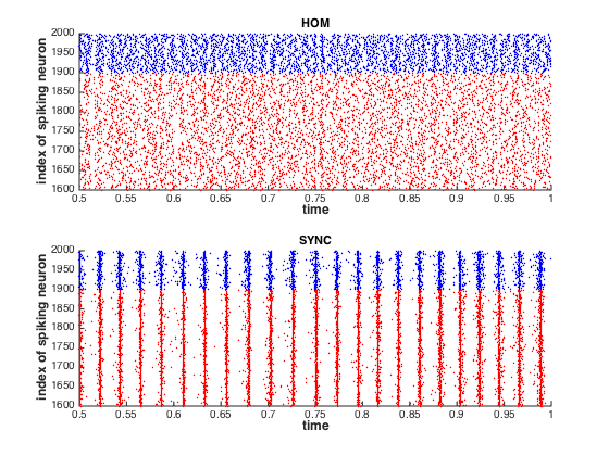
Figure 1. Rastor plot of the central local population of SYN and HOM networks. The drive rate at even-indexed local populations is $\lambda_{Even}=6000$ spikes/sec. The index of neuron $(m,n,k)$ is $[(n-1)M+m](N_{E}+N_{I})+k$.

The three REG networks are much more interesting as we can see different spike count correlations among different local populations when parameters change. With higher $\mathit{ratio}_{E}$ ($\mathit{ratio}_{E}=0.15$), the spike activities in all $9$ blocks are largely correlated (Figure 2 middle panel). When $\mathit{ratio}_{E}=0.05$, much less correlation is seen. And the rastor plot also looks less synchronized (Figure 2 left panel). If the long range connectivity remains $\mathit{ratio}_{E}=0.15$ but we drive odd-indexed local populations only half strong as even-indexed local populations, the spike count correlation is between the previous two cases (Figure 2 right panel). From the three rastor plots presented in Figure 2, we can conclude that both stronger long range connectivity and more homogeneous drive rate contribute to a more correlated spiking pattern among different local populations. A natural question is how such correlated spiking activity changes when two local populations that are further apart. We will extensively investigate this problem in Section 6.

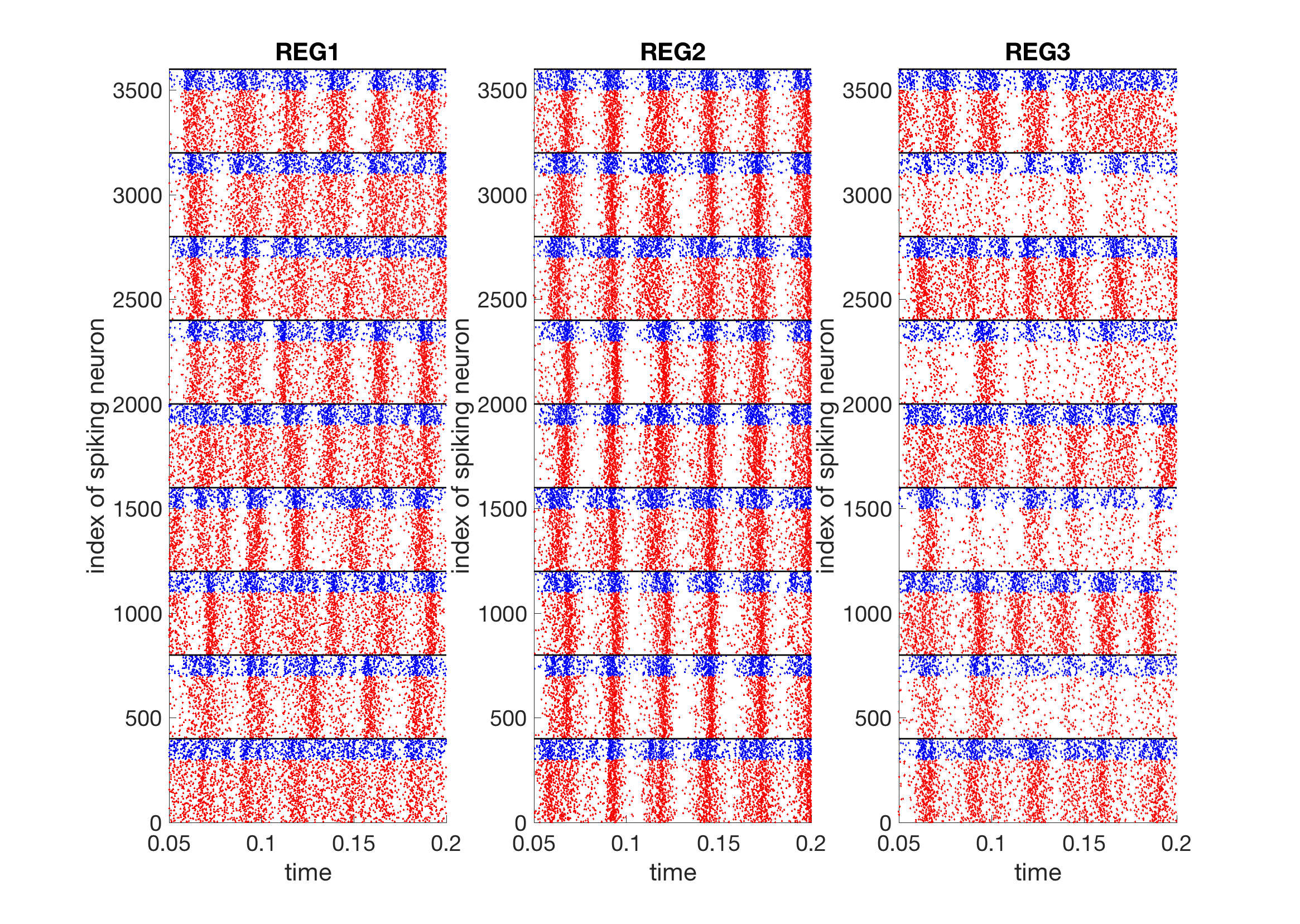
Figure 2. Rastor plot of the full population of three REG networks. The drive rate at even-indexed local populations is $\lambda_{Even}=6000$ spikes/sec. The index of neuron $(m,n,k)$ is $[(n-1)M+m](N_{E}+N_{I})+k$.

It remains to comment on the firing rate. The mean firing rate of the central block is presented in Figure 3. The drive rate of even-indexed population varies from $\lambda_{Even}=1000$ to $\lambda_{Even}=8000$. Different from our previous result in [14], the synchronized network SYN now fires a lower rate when the external drive is very strong. We believe the reason is that inhibitory kicks in paper [14] are voltage-dependent. As a result, when the spiking activity is very synchronized, a neuron tends to receive lots of inhibitory kicks when it just jumps out from state $\mathcal{R}$ (i.e., low membrane potential). Hence the effective inhibitory current in the synchronized network in [14] is weaker, which contributes to a higher firing rate there.

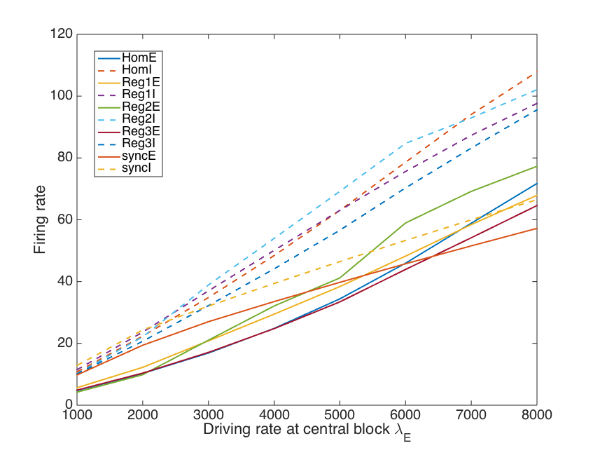
Figure 3. Mean firing rate at the central local population verses $\lambda_{Even}$ for all five networks. The drive rate at even-indexed local populations increases from $\lambda_{Even}=1000$ spikes/sec to $8000$ spikes/sec.

5. Comparing firing rates with mean-field approximations

The aim of this section is to study the mean-field-type approximations of the network model. Two reduced models with exactly solvable mean firing rates are proposed in Section 5.1 and 5.2. In Section 5.3, we compare the mean firing rate produced by these reduced models with the empirical firing rate of the network model, and analyze the discrepancy between these firing rates.

5.1. Reduced linear model

Similarly as in the reduced models for a homogeneous population of neurons studied in [14], we assume that the membrane potential of each neuron $i$ changes at a constant speed and resets from $1$ to $0$ after firing without refractory state,

(5.1) $$\frac{dv}{dt}=F^{+}-F^{-},\quad\text{for $v\in$ [0,1]},$$

where $F^{+}$ and $F^{-}$ are forces that drive membrane potential upward and downward respectively. In particular, with respect to the quantities defined previously, we have

(5.2) $$C_{EE}=N_{E}P_{EE}S_{EE},\qquad C_{IE}=N_{E}P_{IE}S_{IE},$$

$$C_{EI}=N_{I}P_{EI}S_{EI},\qquad C_{II}=N_{I}P_{II}S_{II},$$

$$D_{EE}=N_{E}\rho_{EE}S_{EE},\qquad D_{IE}=N_{E}\rho_{IE}S_{IE},$$

$$D_{EI}=N_{I}\rho_{EI}S_{EI},\qquad D_{II}=N_{I}\rho_{II}S_{II}.$$

We can then define upward and downward drifting speed for excitatory neurons in local population $L_{m,n}$ as

(5.3) $$F^{+} = \frac{1}{M}\left(f^{E}_{m,n}C_{EE}+\sum_{(m^{\prime},n^{\prime})\in\mathcal{N}(m,n)}f^{E}_{m^{\prime},n^{\prime}}D_{EE}+\lambda^{E}_{m,n}\right),$$

$$F^{-} = \frac{1}{M}\left(f^{I}_{m,n}C_{EI}+\sum_{(m^{\prime},n^{\prime})\in\mathcal{N}(m,n)}f^{I}_{m^{\prime},n^{\prime}}D_{EI}\right),$$

and for inhibitory neurons in local population $L_{m,n}$ as

(5.4) $$F^{+}=\frac{1}{M}\left(f^{E}_{m,n}C_{IE}+\sum_{(m^{\prime},n^{\prime})\in\mathcal{N}(m,n)}f^{E}_{m^{\prime},n^{\prime}}D_{IE}+\lambda^{I}_{m,n}\right)$$

$$F^{-}=\frac{1}{M}\left(f^{I}_{m,n}C_{II}+\sum_{(m^{\prime},n^{\prime})\in\mathcal{N}(m,n)}f^{I}_{m^{\prime},n^{\prime}}D_{II}\right)\,.$$

As introduced in the previous chapter, $f^{E}_{m,n}$ and $f^{I}_{m,n}$ are mean excitatory and inhibitory firing rates for local population $L(m,n)$. Since we assume each population $L_{m,n}$ to be homogenous, self-consistency results in an explicit expression of firing rates, which can be derived in a similar way as in [14]. To be precise, the above mentioned linear system can be expressed by the form $\mathbf{A}\mathbf{f}=\mathbf{b}$, where $\mathbf{f}$ and $\mathbf{b}$ are

(5.5) $$\mathbf{f}=\begin{pmatrix}f^{E}_{1,1}\\ f^{I}_{1,1}\\ f^{E}_{1,2}\\ f^{I}_{1,2}\\ \ldots\\ f^{E}_{m,n}\\ f^{I}_{m.n}\end{pmatrix}\qquad\mathbf{b}=-\begin{pmatrix}\lambda^{E}_{1,1}\\ \lambda^{I}_{1,1}\\ \lambda^{E}_{1,2}\\ \lambda^{I}_{1,2}\\ \ldots\\ \lambda^{E}_{m,n}\\ \lambda^{I}_{m.n}\end{pmatrix},$$

and $\mathbf{A}$ can be derived using (5.3) to (5.4).

For example, if $M=N=2$, the coefficient matrix $\mathbf{A}$ is

(5.6) $$\begin{pmatrix}C_{EE}-M&-C_{EI}&D_{EE}&-D_{EI}&D_{EE}&-D_{EI}&0&0\\ C_{IE}&-C_{II}-M&D_{IE}&-D_{II}&D_{IE}&-D_{II}&0&0\\ D_{EE}&-D_{EI}&C_{EE}-M&-C_{EI}&0&0&D_{EE}&-D_{EI}\\ D_{IE}&-D_{II}&C_{IE}&-C_{II}-M&0&0&D_{IE}&-D_{II}\\ D_{EE}&-D_{EI}&0&0&C_{EE}-M&-C_{EI}&D_{EE}&-D_{EI}\\ D_{IE}&-D_{II}&0&0&C_{IE}&-C_{II}-M&D_{IE}&-D_{II}\\ 0&0&D_{EE}&-D_{EI}&D_{EE}&-D_{EI}&C_{EE}-M&-C_{EI}\\ 0&0&D_{IE}&-D_{II}&D_{IE}&-D_{II}&C_{IE}&-C_{II}-M\end{pmatrix}\,.$$

The explicit form of $\mathbf{A}$ gets complicated quickly with more populations. But the solution of firing rates always exists whenever the coefficient matrix $\mathbf{A}$ is invertible. By the perturbation theory of matrices, it is easy to see that $\mathbf{A}$ is invertible if matrix

$$\begin{bmatrix}C_{EE}-M&-C_{EI}\\ C_{IE}&-C_{II}-M\end{bmatrix}$$

is invertible and the coupling strengths $\rho_{Q_{1}Q_{2}}$ are sufficiently small for $Q_{1},Q_{2}\in\{E,I\}$.

5.2. Reduced quadratic model

A reduced quadratic model can be built upon the reduced linear model in a similar way, with a slight improvement by including a fixed refractory period after each firing event. Namely, the normalized membrane potential satisfies the same drift condition described in (5.1), except that whenever $V$ resets from $1$ to $0$, it stays at $0$ for a fixed amount of refractory time $\tau_{\mathcal{R}}$ before resuming its linear climb.

Using the self-consistency condition again, we now derive a system of quadratic equations for the excitatory and inhibitory firing rates $f^{E}_{m,n}$ and $f^{I}_{m,n}$ of population $L_{m,n}$ as follows,

(5.7) $$Mf^{E}_{m,n}=\left(1-\tau_{\mathcal{R}}f^{E}_{m,n}\right)$$

$$\hskip 50.58878pt\left(f^{E}_{m,n}C_{EE}+\sum_{(m^{\prime},n^{\prime})\in\mathcal{N}(m,n)}f^{E}_{m^{\prime},n^{\prime}}D_{EE}+\lambda^{E}_{m,n}-f^{I}_{m,n}C_{EI}-\sum_{(m^{\prime},n^{\prime})\in\mathcal{N}(m,n)}f^{I}_{m^{\prime},n^{\prime}}D_{EI}\right)$$

$$Mf^{I}_{m,n}=\left(1-\tau_{\mathcal{R}}f^{I}_{m,n}\right)$$

$$\hskip 50.58878pt\left(f^{E}_{m,n}C_{IE}+\sum_{(m^{\prime},n^{\prime})\in\mathcal{N}(m,n)}f^{E}_{m^{\prime},n^{\prime}}D_{IE}+\lambda^{I}_{m,n}-f^{I}_{m,n}C_{II}-\sum_{(m^{\prime},n^{\prime})\in\mathcal{N}(m,n)}f^{I}_{m^{\prime},n^{\prime}}D_{II}\right).$$

Lemma 5.1.

Suppose that the reduced quadratic model has a unique solution $\mathbf{f}$ when $\tau_{\mathcal{R}}=0$. Then for sufficiently small $\tau_{\mathcal{R}}>0$, equation (5.7) admits a solution near $\mathbf{f}$.

Proof.

Using notations from linear reduced model, we can write the above quadratic system as

(5.8) $$\mathbf{A}\mathbf{x}+\tau_{\mathcal{R}}f(\mathbf{x})=b,$$

where $\tau_{\mathcal{R}}f(\mathbf{x})$ corresponds to the small perturbation of quadratic terms. Assuming that $\mathbf{A}$ is invertible and the linear system has a solution, we can define a new function on $\mathbb{R}^{2MN}$ as

$$g(\mathbf{x})=\mathbf{A}^{-1}\left(\mathbf{A}\mathbf{x}+\tau_{\mathcal{R}}f(\mathbf{x}+\mathbf{f})-\mathbf{b}\right)+\mathbf{A}^{-1}\mathbf{b}=\mathbf{x}+\tau_{\mathcal{R}}\mathbf{A}^{-1}f(\mathbf{x}+\mathbf{f}),$$

where $\mathbf{f}$ is the solution when $\tau_{\mathcal{R}}=0$. Notice that (5.2) is the identity function when $f(\mathbf{x})=0$. Consider the function $f$ within the hypercube $[-1,1]^{2MN}$, we have $\|f(\mathbf{x}+\mathbf{f})\|<c$ for some constant $c$ depending on parameters. Therefore, for sufficiently small $\tau_{\mathcal{R}}$, $\|\mathbf{A}^{-1}f(\mathbf{x}+\mathbf{f})\|<1$ for all $\mathbf{x}\in[-1,1]^{2MN}$. This means that for all $\hat{\mathbf{x}}:=(x_{1},\ldots,x_{i-1},-1,x_{i},\ldots,x_{2MN}),\text{ and }\tilde{x}:=(x_{1},\ldots,x_{i-1},1,x_{i},\ldots,x_{2MN})\in[-1,1]^{2MN}$, where $i\in\{1,2,\ldots,2MN\}$,

$$g_{i}(\hat{\mathbf{x}})=-1+\tau_{\mathcal{R}}A^{-1}f(\hat{\mathbf{x}}+\mathbf{f})(i)<0,$$

$$g_{i}(\tilde{\mathbf{x}})=1+\tau_{\mathcal{R}}A^{-1}f(\tilde{\mathbf{x}}+\mathbf{f})(i)>0.$$

By Poincare-Miranda theorem, which is a generalization of the intermediate value theorem, $g(\mathbf{x})$ has a zero $\mathbf{x}^{*}$ in the hypercube $[-1,1]^{2MN}$. Using the substitution $\mathbf{y}=\mathbf{x}^{*}+\mathbf{f}$, we can easily derive that $\mathbf{A}\mathbf{y}+\tau_{\mathcal{R}}f(\mathbf{y})=\mathbf{b}$. ∎

5.3. Analysis and Comparison

We compare the firing rate predictions of the reduced linear and quadratic models against our stochastic network model in all five chosen networks with varying degrees of synchronization. For the sake of simpler notation, we denote the firing rate from stochastic model by $f^{Q}_{m,n}$, and that from linear and quadratic models by $\tilde{f}^{Q}_{m,n}$ and $\hat{f}^{Q}_{m,n}$ respectively, where $Q\in\{E,I\}$. We define the mean relative errors of linear and quadratic predictions to be

$$\tilde{REL}^{Q}:=\frac{1}{MN}\sum_{m,n}\frac{f^{Q}_{m,n}-\tilde{f}^{Q}_{m,n}}{f^{Q}_{m,n}},\qquad\hat{REL}^{Q}:=\frac{1}{MN}\sum_{m,n}\frac{f^{Q}_{m,n}-\hat{f}^{Q}_{m,n}}{f^{Q}_{m,n}},$$

respectively for $Q\in\{E,I\}$. Note that we do not take absolute value because we would like to discuss the overestimate and underestimate of the mean-field approximations later in this section. Figure 4 plots the relative errors in all five networks in the sequence of HOM, REG1,REG2, REG3, and SYN from left to right. We have two observations from Figure 4: (i) the linear approximation $\tilde{f}^{Q}_{m,n}$ is always smaller than the quadratic approximation $\hat{f}^{Q}_{m,n}$, and (ii) the quadratic approximation tends to underestimate the mean firing rate when the partial synchronization is weak and overestimate when a strongly drived network is very synchronized.

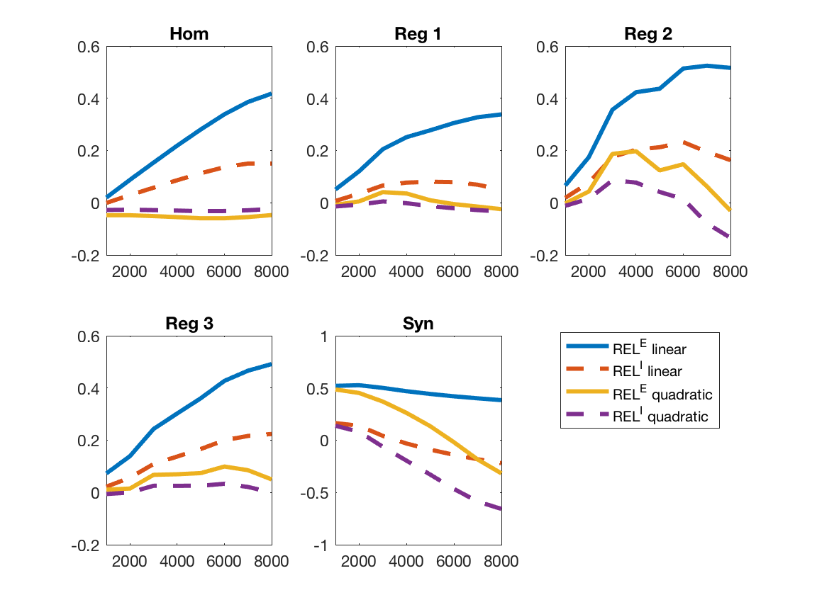
Figure 4. Relative errors of excitatory and inhibitory firing rate predictions for both linear and quadratic models in all five networks. The sequence of networks are HOM, REG1, REG2, REG3, and SYN from left to right. The driving rate increases from $\lambda=1000$ spikes/sec to $8000$ spikes/sec.

The mechanism of the first observation is simple. Similarly as in our previous paper [14], the inhibitory firing rate is always significantly higher than the excitatory firing rate, leading to a larger fraction of inhibitory kicks being missed during refractory than excitatory kicks. This causes the neuron system to be more excited in the quadratic model than in the linear model without refractory.

It remains to discuss the discrepancy between the empirical mean firing rate and the mean-field approximation in each network. We found that the reduced quadratic model gives decent approximation when the network has weak synchronizations, i.e., examples HOM, REG1, and REG3. On the other hand, when the network becomes more synchronous, one observes significant discrepancy between the network model and its mean-field approximation (examples REG2 and SYN). Different from the numerical result in [14], the reduced quadratic model overestimates the mean firing rate when the network is in a strong synchronization. This can be seen from the plot of SYN network and REG2 network with strong driving in Figure 4.

We conclude that such discrepancy is caused by the partial synchronous spiking activity during multiple firing events. The derivation of both mean-field models relies on the assumption that the arrival of postsynaptic kicks is homogeneous in time, which is clearly violated during synchronous spiking activities. Right after a multiple firing event, many neurons will stay at $\mathcal{R}$ and be irresponsive to incoming postsynaptic kicks. As a result, a disproportionately large fraction of postsynaptic kicks are missed in a few ms after a large spiking volley. As demonstrated in Figure 5, the percentage of missed synaptic input is higher than the percentage of time spend in refractory in all network examples. This “additional fraction” of missing spike is not negligible in network REG2 and significant in network SYN.

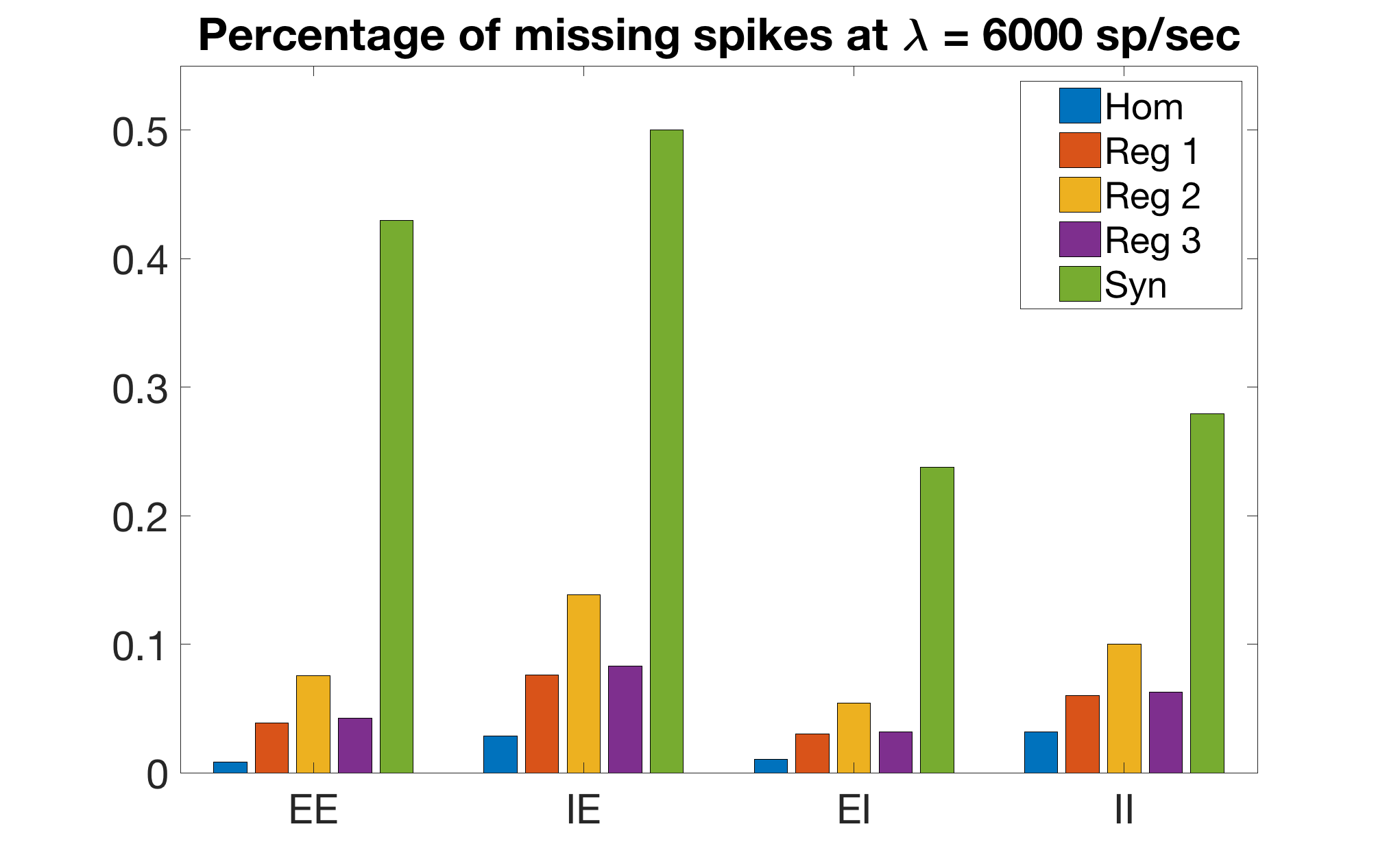
Figure 5. The “additional fraction” of missing E-E, E-I, I-E, and I-I spikes in all five network examples. “Additional fraction” means the percentage of missing $Q_{1}-Q_{2}$ spikes subtracts the average percentage of time that a postsynaptic neuron of the type $Q_{2}$ spends at the refractory, where $Q_{1},Q_{2}\in\{E,I\}$. All missing spike percentages are averaged over$9$ local populations.

For $Q_{1},Q_{2}\in\{E,I\}$, let $\epsilon^{Q_{1}Q_{2}}_{m,n}$ be the percentage of “additional” missing spikes, which means that the average percentage of time duration for neuron $Q_{2}$ staying at the refractory is subtracted from the empirical missing spikes proportions. Let $\Delta F^{E}_{m,n}$ be the net gain of excitatory current as compared with the reduced model. In the regime when the quadratic approximation $\hat{f}^{Q}_{m,n}$ remains a good approximation of the network firing rate $f^{Q}_{m,n}$, we have

$$\Delta F^{E}_{m,n} \approx \left(\epsilon^{EI}_{m,n}f^{I}_{m,n}C_{EI}+\sum_{(m^{\prime},n^{\prime})\in\mathcal{N}(m,n)}\epsilon^{EI}_{m^{\prime},n^{\prime}}f^{I}_{m^{\prime},n^{\prime}}D_{EI}\right)$$

$$-\left(\epsilon^{EE}_{m,n}f^{E}_{m,n}C_{EE}+\sum_{(m^{\prime},n^{\prime})\in\mathcal{N}(m,n)}\epsilon^{EE}_{m^{\prime},n^{\prime}}f^{E}_{m^{\prime},n^{\prime}}D_{EE}\right)\,.$$

Similarly, we have the net gain of inhibitory current is given by

$$\Delta F^{I}_{m,n} \approx \left(\epsilon^{II}_{m,n}f^{I}_{m,n}C_{II}+\sum_{(m^{\prime},n^{\prime})\in\mathcal{N}(m,n)}\epsilon^{II}_{m^{\prime},n^{\prime}}f^{I}_{m^{\prime},n^{\prime}}D_{II}\right)$$

$$-\left(\epsilon^{IE}_{m,n}f^{E}_{m,n}C_{IE}+\sum_{(m^{\prime},n^{\prime})\in\mathcal{N}(m,n)}\epsilon^{IE}_{m^{\prime},n^{\prime}}f^{E}_{m^{\prime},n^{\prime}}D_{IE}\right)\,.$$

Note that the missing percentage of excitatory postsynaptic kicks is usually higher than that of the I kicks, partially due to the longer synapse delay time of I-kicks. Put empirical missing percentages and constants in all five network examples into expressions $\Delta F^{E}_{m,n}$ and $\Delta F^{I}_{m,n}$. We can see that when $f_{I}^{m,n}$ is significantly larger (at least $1.5$ times larger) than $f_{E}^{m,n}$, we have positive net gain for both empirical $E$ and empirical $I$ current, corresponding to the underestimate of the quadratic model.

However, when the network is very synchronous, all neurons spike in a semi-periodic way, and $\hat{f}^{Q}_{m,n}$ can be very far away from $f^{Q}_{m,n}$. In this regime, we find that the firing rate is simply approximated by

$$\bar{f}^{E}_{m,n}=\bar{f}^{I}_{m,n}\approx\frac{1}{\frac{M}{\lambda_{m,n}}+\tau_{\mathcal{R}}}\,,$$

where $\lambda_{m,n}=\lambda^{E}_{m,n}=\lambda^{I}_{m,n}$. In other words, in network SYN, the firing activity is so synchronized that most neurons participate in a multiple firing event, and restart from the refractory right after it. The accuracy of this estimate is presented in Figure 6, in which we calculate the mean relative error $\overline{REL}^{Q}$ in the same way as calculating $\tilde{REL}^{Q}$ and $\hat{REL}^{Q}$ and plot it at different drive rates. We can see that $\overline{REL}^{Q}$ gives a better approximation of the mean firing rate of SYN network, especially for excitatory local populations. Comparing $\bar{f}^{Q}_{m,n}$ with $\hat{f}^{Q}_{m,n}$, we find that the quadratic formula underestimates the mean firing rate at low drive, and overestimates it at high drive. This mechanism also partially explains the overestimate of the quadratic formula in network REG2 at high drive rate, at which synchronization is also very significant.

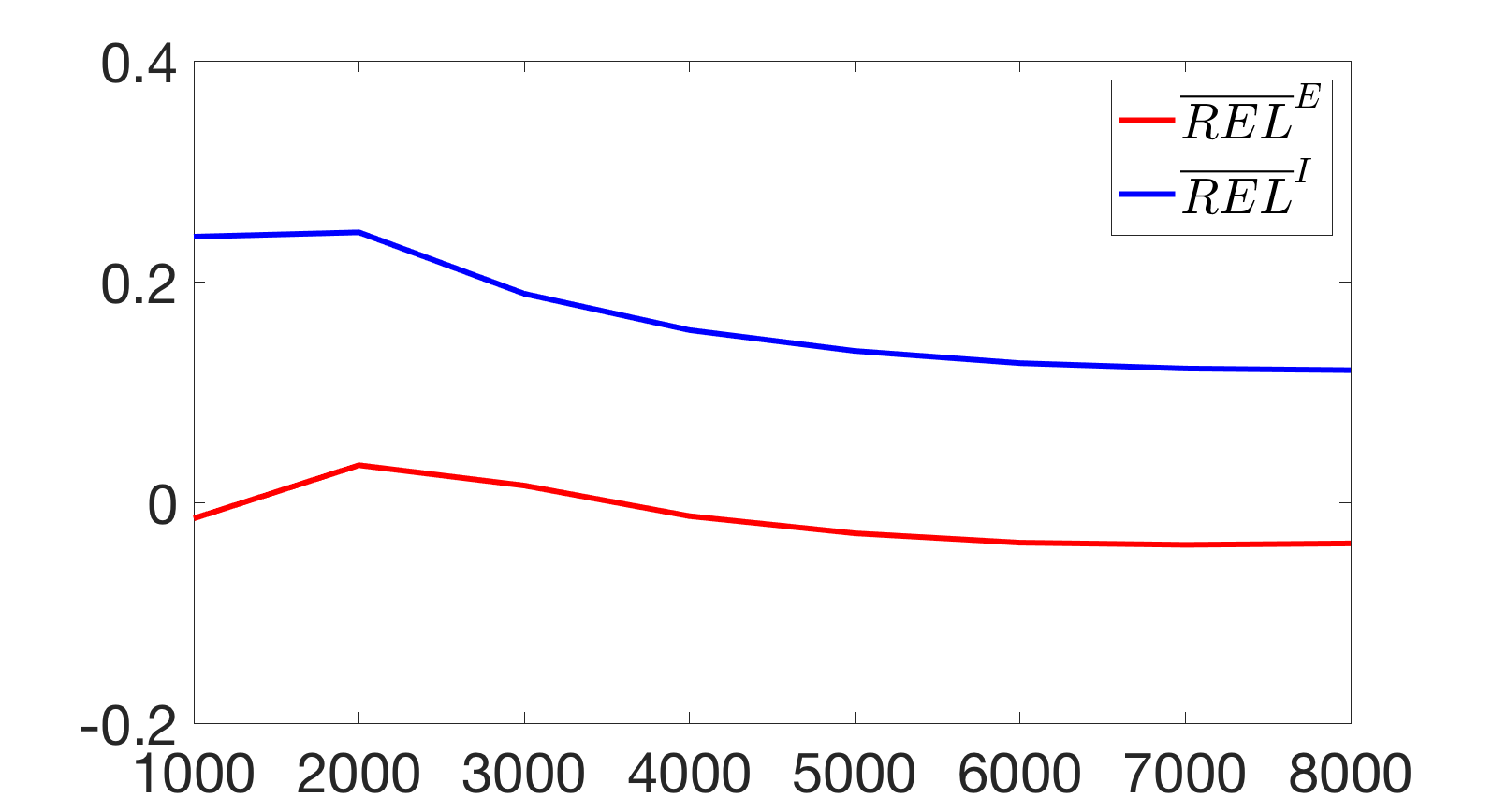
Figure 6. The total relative error $\overline{REL}^{E}$ and $\overline{REL}^{I}$ by assuming that the network is periodic.

Further numerical analysis shows that this $\bar{f}^{Q}_{m,n}$ actually has overestimate and underestimate that significantly cancel each other. $\bar{f}^{Q}_{m,n}$ overestimates the mean firing rate in a way that many pending inhibitory kicks can survive after the refractory, and underestimates the mean firing rate because a synchronous spiking event occurs when some membrane potential reaches $M$, at which time the mean membrane potential is still well below $M$. We note that such analysis for a very synchronized network is not given in our previous paper [14], as the network SYN in this paper is much more synchronous than examples there.

6. Spatial correlation of spike volleys

The semi-synchronized bursts of neuron spikes, i.e., the multiple firing events, observed in Figure 2 are consistent with our experimental results and numerical results [6, 17, 18]. The scale of a multiple firing event and the time interval between two consecutive events may vary. This is an emergent phenomenon that is different from the total synchronization studied in [2, 3, 1]. It is believed that such semi-synchronized burst is related to the gamma rhythm in our brain [1, 10], and is resulted by the interplay of excitatory and inhibitory populations, which is a milder version of the PING mechanism [2]. Inhibitory (GABAergic) synapses in a population usually act a few milliseconds more slowly than excitatory (AMPA) synapses. As a result, an excitatory spike will excite many postsynaptic neurons quickly and form a cascade, which will be terminated when the pending inhibitory kicks take effect. In [14], we have found that the degree of synchronization is extremely sensitive with respect to small changes of the synapse delay times $\tau_{E}$ and $\tau_{I}$. However, very limited mathematical justification is available so far.

One salient phenomenon observed in our numerical simulations is that spike volleys generated by different local populations are correlated. We call such correlated spiking activity among different local populations the spatial correlation. One interesting observation is that under “reasonable” parameter settings, this correlated spiking activity can only spread to several blocks away. The aim of this section is to investigate two questions: (i) What is the mechanism of this spatial correlation? and (ii) How far away could this spatial correlation spread? We will describe our numerical results about spatial correlation in Section 6.1 and 6.2. The mechanism of spatial correlation will be studied in Section 6.3. A study of the mechanism of correlation decay is provided in Section 6.4.

6.1. Quantifying spatial correlations

The quantification of spatial correlation relies on the ergodicity of the Markov process. It follows from Corollary 3.3 that for any two local populations $(m,n)$ and $(m^{\prime},n^{\prime})$ and any $Q_{1},Q_{2}\in\{E,I\}$, we have well-defined and computable covariance $\mbox{cov}_{T}^{Q_{1},Q_{2}}(m,n;m^{\prime},n^{\prime})$ and Pearson’ correlation coefficient $\rho^{Q_{1},Q_{2}}_{T}(m,n,m^{\prime},n^{\prime})$. By Corollary 3.4, the covariance $\mbox{cov}_{T}(m,n,m^{\prime},n^{\prime})$ and correlation coefficient $\rho_{T}(m,n,m^{\prime},n^{\prime})$ for the total spike count between two local population (regardless the spike type) are also well defined and computable.

We remark that sometimes it makes sense to have different “resolutions” at different spike counts. For example, whether a local population fires $5$ spike or $10$ spikes during a $10$ ms time window makes qualitative difference because we may think $10$ spikes in such a time window gives a multiple firing event. But whether a local population fires $295$ or $300$ spikes in the same time window is less important. To address this, we can prescribe a mapping on the spike count during $[0,T]$. Let $\bm{\xi}=\{\xi_{1},\cdots,\xi_{k}\}\subset\mathbb{N}_{+}$ be a “dictionary”. Let $f_{\bm{\xi}}:\mathbb{N_{+}}\mapsto\{1,\cdots,k+1\}$ be a function such that

$$f_{\bm{\xi}}(n)=\left\{\begin{array}[]{ccc}\max\{1\leq i\leq k\,|\,n\leq\xi_{i}\}&\mbox{ if }&n\leq\xi_{k}\\ k+1&\mbox{ if }&n>\xi_{k}\end{array}\right.$$

When starting from the steady state $\pi$, we have random variables $f_{\bm{\xi}}(N^{Q}_{m,n}([0,T]))$ representing the mapping of the spike count on $[0,T]$. The we can define the covariance $\mbox{cov}_{T,\bm{\xi}}^{Q_{1},Q_{2}}(m,n,m^{\prime},n^{\prime})$ and the Pearson correlation coefficient $\rho^{Q_{1},Q_{2}}_{\bm{\xi},T}(m,n,m^{\prime},n^{\prime})$ in an analogous way. One advantage of using $f_{\bm{\xi}}$ to define the correlation is that $|\bm{\xi}|$ can be much smaller than $N_{E}$ and $N_{I}$. Hence the estimates of covariance and correlation coefficient can be more accurate.

It remains to comment on the size of a time window $T$. An ideal time window should be large enough to contain a spike volley, but not as large as the time between two consecutive time spike volleys. There is no silver lining of time-window size that fits all parameter sets. A (very) rough estimate is that $T$ should be greater than the maximum of $N_{Q}$ i.i.d exponential random variables with mean $\tau_{Q}$, but less than $M/\lambda^{Q}_{m,n}+\tau_{\mathcal{R}}$. It is well known that the maximum of $N_{Q}$ i.i.d exponential random variables with mean $\tau_{Q}$, denoted by $Z$, can be represented as the sum of independent exponential random variables

$$Z=W_{1}+\cdots+W_{N_{Q}}\,,$$

where $W_{k}$ has mean $\frac{\tau_{Q}}{k}$. Hence the expectation of $Z$ is $\tau_{Q}H_{N_{Q}}$, where $\{H_{n}\}$ is the Harmonic number

$$H_{n}=\sum_{k=1}^{n}\frac{1}{k}\,.$$

It is clear that $H_{N_{Q}}\tau_{Q}$ overestimates because a spike volley may not involve all neurons. At the same time, it also underestimates because it takes some time for the cascade of excitatory spikes to excite all neurons participating in a spike volley. But our simulations shows that the qualitative properties of the spatial correlation is not very sensitive with respect to the choice of time-window size. For the parameters of a “regular” network, we have $H_{300}\tau_{EE}\approx 10$ ms. Also we have $M/\lambda_{E}+\tau_{\mathcal{R}}\approx 19$ ms if $\lambda_{E}=6000$ (strong drive). Hence we choose $T=15$ ms in our simulations in the next subsection.

6.2. Spatial correlation decay

Our first key observation is that in many settings, the spatial correlation decays quickly when two local populations are further apart. The aim of this subsection is to describe this numerical finding. We will address possible mechanisms of spatial correlation and spatial correlation decay in the following two subsections.

As discussed in the last subsection, we choose $T=15$ ms as the size of a time window. Since the qualitative result for the spatial correlation among E-E, E-I .etc are the same, we select $\rho_{T}(m,n,m^{\prime},n^{\prime})$ as the metrics of the spatial correlation. The cases of $\rho^{E,E}_{T}(m,n,m^{\prime},n^{\prime})$ have little difference.

In order to effectively simulate large scale neural fields in which two local populations can be far apart, we choose to study an $1$-D network with $M=1$. The length of array is chosen to be $N=22$ in all of our simulations. We will compare the Pearson correlation coefficient between local populations $L_{1,2}$ and $L_{1,k}$ for $k=2,\cdots,21$. The reason of doing this is to exclude the boundary effect at $L_{1,1}$ and $L_{1,N}$. In our simulation, we run $240$ independent long-trajectories of $\Phi_{t}$. In each trajectory, spike counts in $2000$ time windows are collected after the process is stabilized. The result of this simulation is presented in Figure 7. We find that in all five example networks, the spike count correlation decays quickly with increasing distance between local populations. In homogeneous network HOM, correlation is only observed for nearest neighbor local populations. In three regular networks REG1, REG2, and REG3, no significant correlations are observed when two local populations are $4-8$ blocks away. The speed of correlation decay is higher when external drive rates have higher difference (REG1) and when the external connection is weaker (REG3). The synchronized network SYN has the slowest decay rate and obvious fluctuations induced by alternating external drive rate at local populations. If one local population models a hypercolumn in the visual cortex, our simulation suggests that the Gamma wave does not have significant correlation at two locations that are $2-3$ millimeters away. This is consistent with experimental observations.

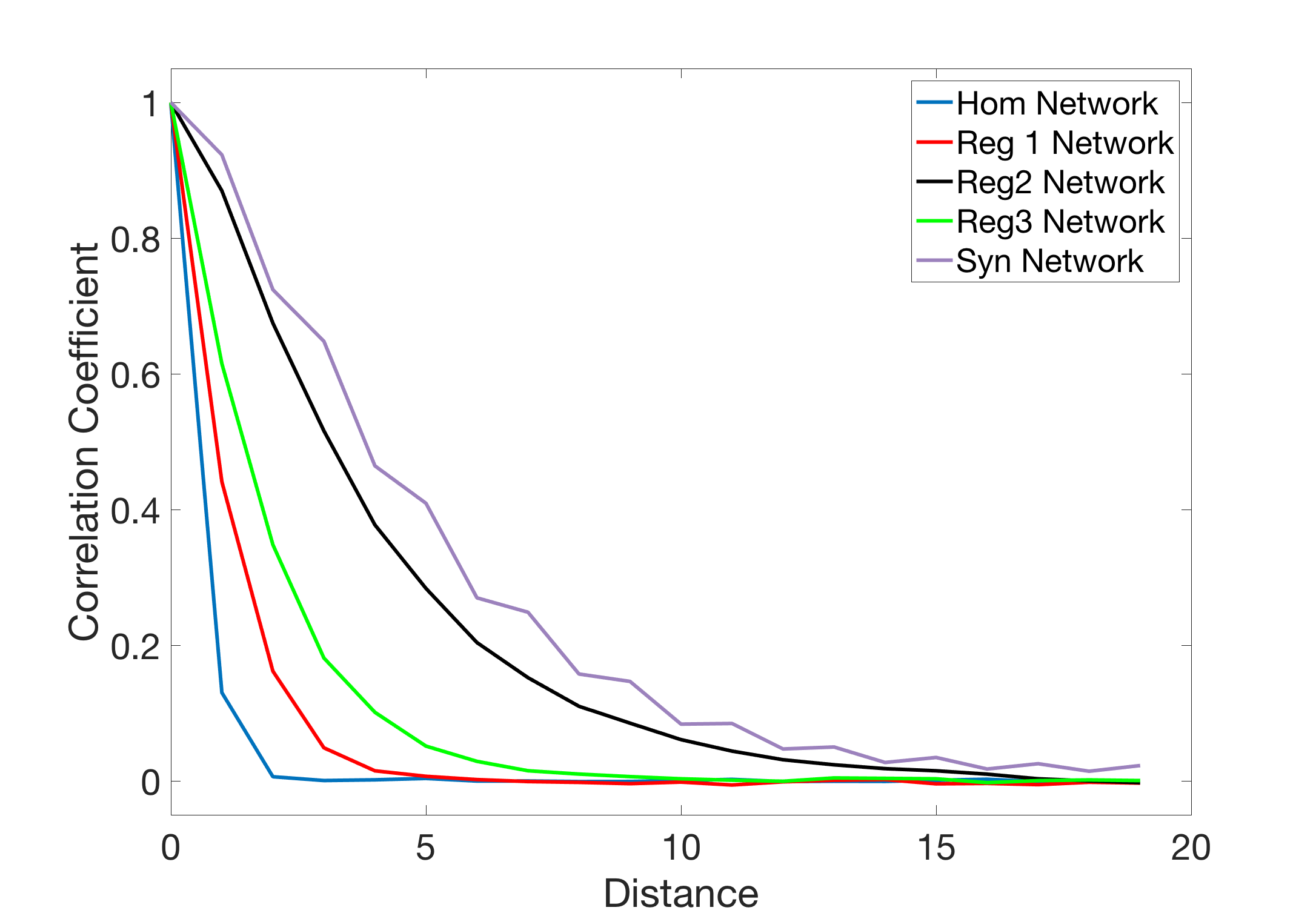
Figure 7. Change of spike count correlation coefficient with increasing distance between to local populations. Correlation coefficients are measured between $L_{1,2}$ and $L_{1,k}$ for $k=2,\cdots,21$ in five example networks.

6.3. Mechanism of spatial correlation

The aim of this section is to investigate the mechanism of spatial correlation, especially the spatial correlation of spike counts between two nearest local populations. We believe that the mechanism of spatial correlation is similar to that of a multiple firing event in a local population. The excitatory neurons stimulate each other and form an avalanche of spikes, which is terminated by the later arrival of inhibitory kicks. Because both excitatory and inhibitory neurons connect to nearest neighbors, two neighbor local populations tend to have spike volleys at the same time.

To better explain this dynamics, we first propose the following $6$-variable ODE system for a qualitative description of what happens during a spike volley at one local population. The main changing parameters in our ODE model are $\tau_{E}$ and $\tau_{I}$. Other parameters like $N_{E}$, $N_{I}$, $S_{EE}$, .etc are same as in the model description. This system contains six variables $G_{E},G_{I},H_{E},H_{I},R_{E}$, and $R_{I}$. Variables $G_{E}$ and $G_{I}$ are the number of excitatory and inhibitory neurons that are located in the “gate area”, which means their membrane potentials lie within one excitatory spike from the threshold. We denote the set of neurons in this “gate area” by $G_{E}$ and $G_{I}$ when it does not lead to confusions. Variables $H_{E}$ and $H_{I}$ are the “effective” number of excitatory and inhibitory neurons who just spiked but the spikes have not taken effects yet. If, for example, $50\%$ of postsynaptic kicks from a neuron spike have already taken effects, the “effective number” of this neuron is $0.5$. Finally, $R_{E}$ and $R_{I}$ are the number of excitatory and inhibitory neurons that are at refractory. Since we only study the dynamics of one spike volley, we assume that a neuron stays at $\mathcal{R}$ after a spike. Let $c_{E},c_{I}$ be two parameters that will be described later, we have the following multiple firing event model that describes the time evolution of $H_{E},H_{I},G_{E},G_{I},R_{E}$, and $R_{I}$.

(6.1) $$\begin{split}\frac{\mathrm{d}H_{E}}{\mathrm{d}t}=&-\tau_{E}^{-1}H_{E}+\tau_{E}^{-1}P_{EE}H_{E}G_{E}+\frac{\lambda_{E}}{S_{EE}}G_{E}\\ \frac{\mathrm{d}G_{E}}{\mathrm{d}t}=&c_{E}\max\{\tau_{E}^{-1}P_{EE}S_{EE}H_{E}+\lambda_{E}-\tau_{I}^{-1}P_{EI}S_{EI}H_{I},0\}\cdot(N_{E}-G_{E}-R_{E})-\\ &\tau_{I}^{-1}P_{EI}\max\{\frac{S_{EI}}{S_{EE}},1\}H_{I}G_{E}-(\tau_{E}^{-1}P_{EE}H_{E}+\frac{\lambda_{E}}{S_{EE}})G_{E}\\ \frac{\mathrm{d}R_{E}}{\mathrm{d}t}=&\tau_{E}^{-1}P_{EE}H_{E}G_{E}+\frac{\lambda_{E}}{S_{EE}}G_{E}\\ \frac{\mathrm{d}H_{I}}{\mathrm{d}t}=&-\tau_{I}^{-1}H_{I}+\tau_{E}^{-1}P_{IE}H_{E}G_{I}+\frac{\lambda_{I}}{S_{IE}}G_{I}\\ \frac{\mathrm{d}G_{I}}{\mathrm{d}t}=&c_{I}\max\{\tau_{E}^{-1}P_{IE}S_{IE}H_{E}+\lambda_{I}-\tau_{I}^{-1}P_{II}S_{II}H_{I},0\}\cdot(N_{I}-G_{I}-R_{I})\\ &-\tau_{I}^{-1}P_{II}\max\{\frac{S_{II}}{S_{IE}},1\}H_{I}G_{I}-(\tau_{E}^{-1}P_{IE}H_{E}+\frac{\lambda_{I}}{S_{IE}})G_{I}\\ \frac{\mathrm{d}R_{I}}{\mathrm{d}t}=&\tau_{E}^{-1}P_{IE}H_{E}G_{I}+\frac{\lambda_{I}}{S_{IE}}G_{I}\end{split}$$

We note that the aim of this ODE system is to qualitatively describe the excitatory-inhibitory interplay, instead of making any precise predictions. The first equation describes the rate of change of $H_{E}$, which decreases with rate $\tau_{E}^{-1}$. The source of input to $H_{E}$ is neurons in the “gate area” $G_{E}$. We assume that neurons in $G_{E}$ have uniformly distributed membrane potentials. The second equation describes the rate of change of neurons in $G_{E}$. The source of $G_{E}$ is neurons that are not at $G_{E}$ or $R_{E}$. We assume that the increase rate of $G_{E}$ is proportional to both the number of relevant neurons and the net current, if the net current is positive. The coefficient is assumed to be a parameter $c_{E}$. We denote the coefficient of proportion as a parameter $c_{E}$. $G_{E}$ decreases because neurons in $G_{E}$ either spike when receiving excitatory input or drop below the “gate area” when receiving inhibitory input. This is represented by the last two terms in the second equation. The third equation is about $R_{E}$, whose increase rate equals the rate of producing new spikes. The case of inhibitory neurons is analogous, represented by the last three equations about $H_{I},G_{I},R_{I}$, where parameter $c_{I}$ stands for the coefficient of net current for inhibitory neurons.

The most salient feature of this ODE system is the very sensitive dependency of “event size” with respect to $\tau_{E}$ and $\tau_{I}$. When $\tau_{I}$ is much larger than $\tau_{E}$, one can expect larger event sizes for both populations. This is demonstrated in Figure 8. We assume that $\tau_{E}=2$ ms and plot the “event sizes” with varying $\tau_{I}$. The initial condition is $H_{E}=0,G_{E}=20,R_{E}=0,H_{I}=0,G_{I}=5$, and $R_{I}=0$. We showed three cases with varying drive rates, where $\lambda_{E}=\lambda_{I}=0,2000$, and $4000$. The “event sizes” of excitatory and inhibitory populations are $R_{E}(T)$ and $R_{I}(T)$ respectively, where $T$ is the minimum of $20$ ms and the first local minimum of $H_{E}(t)$. The reason of looking for the local minimum is because when the network is driven, this ODE model might generate a “second wave” after the first multiple firing event. Figure 8 confirms two observations in our simulation results. First, the “event sizes” of both excitatory and inhibitory populations increase quickly with larger $\tau_{I}$. Second, the network tends to have bigger multiple firing events when it is strongly driven by external signals.

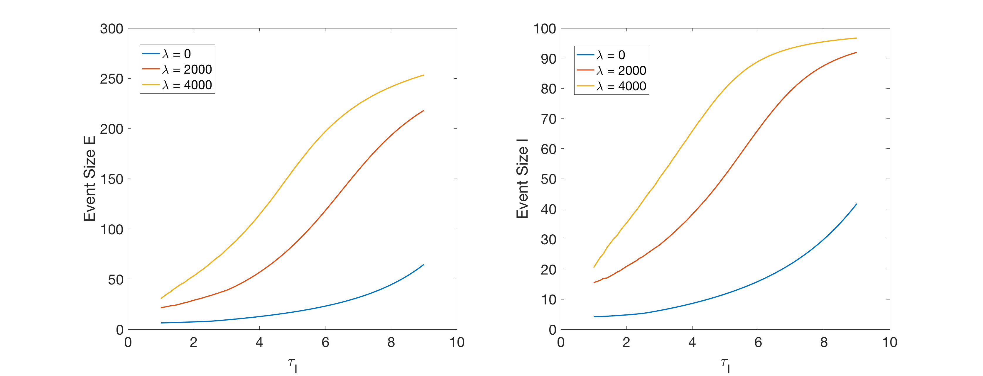
Figure 8. Event size versus $\tau_{I}$ for one local population.

In the limiting senario when $\tau_{I}^{-1}$ is very small, we have the following theorem.

Theorem 6.1.

Assume $\tau_{E}=1$, $\lambda_{E}=\lambda_{I}=0$. Let $\delta_{E}=c_{E}S_{EE}$, $\delta_{I}=c_{E}S_{IE}$, $m=\min\{\delta_{E},P_{EE}\}$,

$$\alpha=P_{EE}N_{E}^{2}e^{-N_{E}m}\,,$$

and

$$\beta=N_{I}(e^{-\delta_{I}N_{E}}+e^{-P_{IE}N_{E}})\,.$$

Assume $N_{E}>m$. Let the initial condition be $(H_{0},0,0,0,0,0)$ for $H_{0}>\alpha$. Then there exist constants $C$ and $T$, such that when $\tau_{I}>C$ and $t>T$, we have $R_{E}(t)>N_{E}-\alpha$ and $R_{I}(t)>N_{I}-\beta$.

Theorem 6.1 implies that as long as $\tau_{I}$ is sufficiently large, even if without external drive, most neurons will eventually spike provided that there are enough pending excitatory spikes in the beginning. Note that $m$ is typically not a very small number ($0.1$ in our simulations). Hence $\alpha$ and $\beta$ are both very small numbers.

The proof of Theorem 6.1 only contains elementary calculations, and we include it in Appendix A.

When many local populations form a $M\times N$ array, an ODE system with $6MN$ variables can be derived from the same approach. We include this ODE system and its description in Appendix B. A direct analysis is too complicated to be interesting. But the numerical result reveals the mechanism of spatial correlation. For the sake of simplicity we consider two local populations, say populations $L_{1,1}$ and $L_{1,2}$. Assume that the local population $L_{1,1}$ is ready for a multiple firing event with initial condition $H_{E}=1,G_{E}=30,R_{E}=0,H_{I}=0,G_{I}=10,R_{I}=0$, while $L_{1,2}$ has a very different profile with $H_{E}=0,G_{E}=10,R_{E}=0,H_{I}=0,G_{I}=2,R_{I}=0$. We further assume that $\tau_{E}=2$ ms and $\lambda_{E}=\lambda_{I}=0$. It is easy to see that without $L_{1,1}$, $L_{1,2}$ will not have any spikes because it is not driven. We compare the “event size” of excitatory and inhibitory populations at $L_{1,1}$ and $L_{1,2}$, which is measured at time $T=20$ ms. This is demonstrated in Figure 9. With strong connectivity $\mbox{ratio}_{E}=0.15$, the multiple firing event at local population $L_{1,1}$ will induce a multiple firing event at local population $L_{1,2}$, even if local population $L_{1,2}$ has much fewer neurons at the “gate area”.

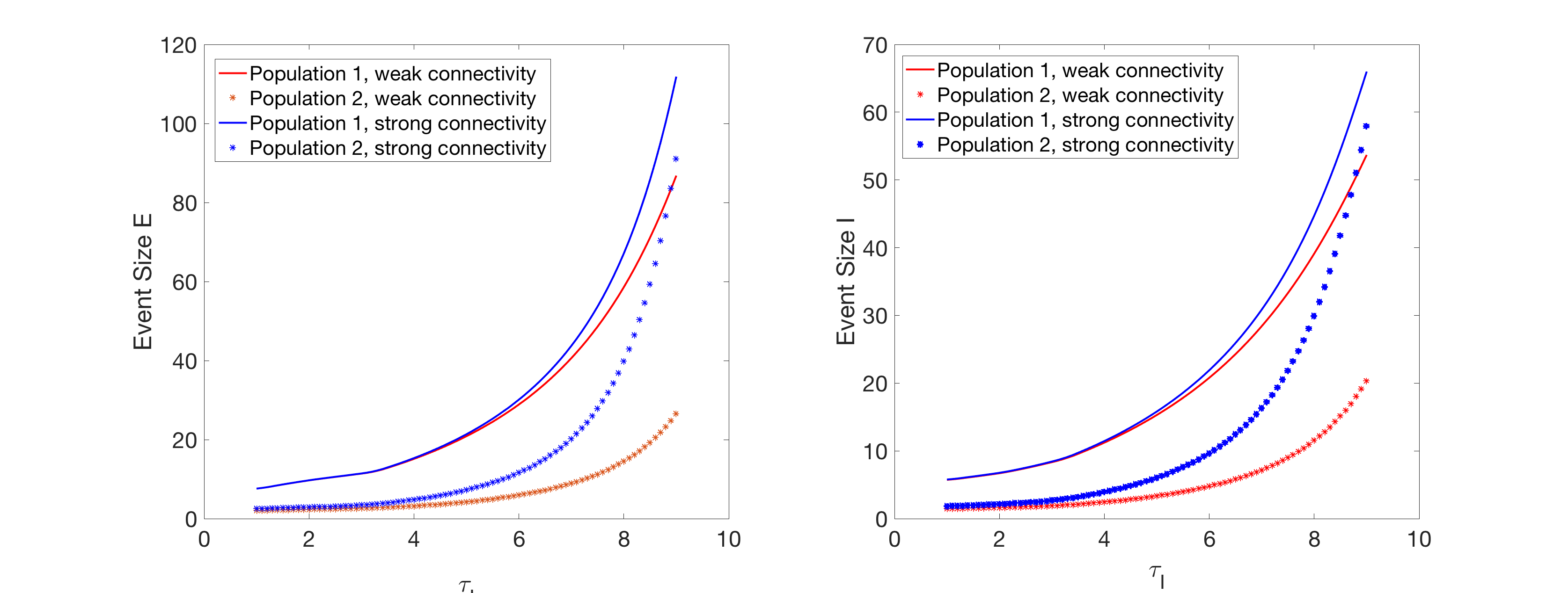
Figure 9. Event size versus $\tau_{I}$ for two local populations.

We believe that this is the mechanism of spike count spatial correlation in our model. When a multiple firing event occurs in one local population, it sends excitatory and inhibitory input to its neighboring local populations. If the membrane potential of a neighboring local population is properly distributed, a multiple firing event will be induced by the activity at its neighbor. Similar to the case of one local population, the size of a multiple firing event sensitively depends on the excitatory and inhibitory synapse delay times.

6.4. Mechanism of spatial correlation decay

In the previous section we have shown that a strong multiple firing event in a local population is very likely to induce a multiple firing event at its neighboring local populations. This partially explains the mechanism of the spatial correlation of spike volley that we have observed. Our final task is to investigate the mechanism of spatial correlation decay, as described in Figure 7, where the spatial correlation of spike volley can only spread to several local populations away.

Why the spatial correlation can not spread to very far away? We believe that (at least in this model) such correlation decay is due to the volatility of spike count in a multiple firing event. Since each neuron finds its postsynaptic neurons in a random way, the spike count in a local population usually has large variance. The variance will be even larger if the external drive rate is heterogeneous. Therefore, even if the initial distributions of the membrane potential and the external drive rates are identical throughout all local populations, the voltage distribution will be very different after the first multiple firing event. Therefore, the next spike volley in different local populations will be less coordinated, which destroys the synchronization. We believe this high volatility of spike volley size significantly contributes to the spatial correlation decay. As shown in Figure 7, in examples REG1 and REG2, $\lambda^{E}_{m,n}$ and $\lambda^{I}_{m,n}$ have very small difference in different local populations. But the spatial correlation decay is still strong. This also explains why the SYN network has the weakest spatial correlation decay. When the size of a spike volley is closer to the size of the entire population, there will be much less variation in the after-event voltage distribution. Hence the voltage distributions in different local populations are relatively similar in a SYN network, which contributes to the observed slow decay of spatial correlation.

This explanation is supported by both analytical calculation and numerical simulation result. We did the following numerical simulation to investigate the volatility of “event size”. Assume $M=N=1$, $\lambda_{E}=\lambda_{I}=3000$, and the initial voltage distribution is generated in the following way: With probability $0.2$, the neuron membrane is uniformly distributed on $\{0,1,\cdots,80\}$. With probability $0.8$, the neuron membrane potential takes the integer part of a normal random variable with mean $0$ and standard deviation $20$. This initial voltage distribution roughly mimics the voltage distribution after a large spike volley. The synapse delay times are $\tau_{E}=2$ ms and $\tau_{I}=1\sim 9$ ms. For each $\tau_{I}=1.0,1.1,\cdots,9.0$, we simulate this model repeatedly for $10000$ times and count the number of excitatory spikes of the first multiple firing event. Then we plot the mean event size and the coefficient of variation (standard deviation divided by mean) of the spike count samples for each $\tau_{I}$. Note that the coefficient of variation is a better metrics than the standard deviation as it is a dimensionless number that measures the relative volatility of a multiple firing event.

This numerical result is shown in Figure 10. We can see that when $\tau_{I}$ become larger, the event size increases and the coefficient of variation decreases. The reason of decreasing is because the size of a multiple firing event usually can not be much larger than the number of neurons. Only a small number of neurons have the chance to spike twice in a multiple firing event, even if in the most synchronized network. The change of coefficient of variation partially explains the observation in Figure 7, in which the decay of spatial correlation is slower when the $\tau_{I}$-to-$\tau_{E}$ ratio is larger (means the network is more synchronized).

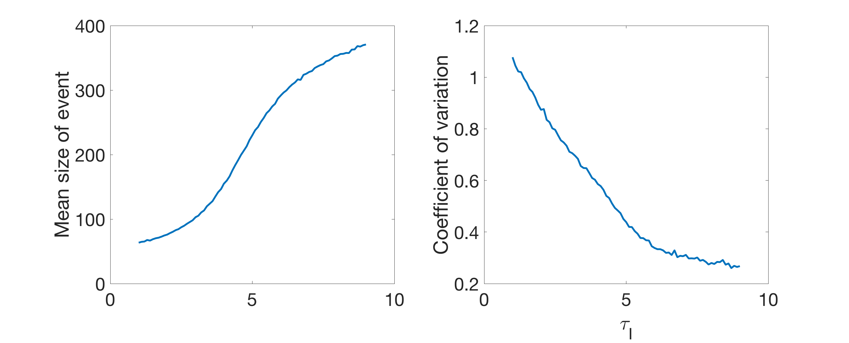
Figure 10. Left: Mean event size versus $\tau_{I}$. Right: Coefficient of variation versus $\tau_{I}$.

It is difficult to directly study the event size on the population model. But it is easy to build a simplified model to study the mechanism of the high variance of multiple firing events. As explained before, a multiple firing event is produced by the recurrent excitation and the slower onset of the inhibition. Therefore, we consider modeling the multiple firing event by stopping a Galton-Watson branching process at a random time. For the sake of simplicity, we only consider the case of $E$ population. Some calculation for a Galton-Watson process will qualitatively explain the reason of high coefficient of variation of sizes of multiple firing events.

Let $X_{i}\sim B(N_{E},p)$ be i.i.d Binomial random variables that represent the numbers of new excitatory spike stimulated by an excitatory spike. Let $Z_{n}$ be a branching process such that $Z_{0}=1$ and

$$Z_{n+1}=X_{1}+\cdots+X_{Z_{n}}\,.$$

Further let the total number of spikes before step $n$ be $S_{n}=Z_{1}+\cdots+Z_{n}$.

Let $T$ be a positive integer-valued random variable that is independent of all $X_{i}$ and $Z_{i}$. $T$ is the approximate onset time of network inhibition. We further assume that $T$ has mean $\mu_{T}$ and variance $\sigma_{T}^{2}$. The approximate event size is then $S_{T}$.

$$S_{T}=Z_{1}+\cdots+Z_{T}\,.$$

Let

$$\mbox{CV}(X)=\frac{\sqrt{\mathbb{E}[(X-\mathbb{E}[X])^{2}]}}{\mathbb{E}[X]}$$

be the coefficient of variation of a positive-valued random variable $X$. The following proposition is straightforward.

Proposition 6.2.

Assume $T$ has finite moment generating function $M_{T}(t)$ for $t>2\log\mu$. Let $\sigma^{2}=N_{E}p(1-p)$ and $\mu=N_{E}p$. We have

$$\mbox{CV}(S_{T})\geq\frac{\sigma\sqrt{\mu-1}}{\mu\sqrt{\mu+1}}\,.$$

Proof.

The proof follows from straightforward elementary calculations. By the property of the Galton-Watson process, we have

$$\mathbb{E}[Z_{n}]=\mu^{n}$$

and

$$\mbox{Var}[Z_{n}]=\mu^{n-1}\sigma^{2}(1+\mu+\cdots+\mu^{n-1})\geq\mu^{2n-2}\sigma^{2}\,.$$

In addition, for $n\geq m$ we have

$$\mbox{cov}(Z_{m},Z_{n}) = =\mathbb{E}[Z_{m}Z_{n}]-\mathbb{E}[Z_{m}]\mathbb{E}[Z_{n}]$$

$$= \mu^{n-m}\mathbb{E}[Z_{m}^{2}]-\mu^{m+n}$$

$$\geq \mu^{n-m}\mathbb{E}[Z_{m}]^{2}-\mu^{m+n}=0\,$$

Therefore, we have

$$\mathbb{E}[S_{n}]=\sum_{k=1}^{n}\mu^{k}=\frac{\mu^{n+1}-1}{\mu-1}$$

and

$$\mbox{Var}[S_{n}] \geq \sum_{k=1}^{n}\mbox{Var}[Z_{k}]$$

$$= \sigma^{2}(1+\cdots+\mu^{2n-2})=\sigma^{2}\frac{\mu^{2n}-1}{\mu^{2}-1}\,.$$

By the law of total expectation,

$$\mathbb{E}[S_{T}]=\mathbb{E}[\frac{\mu^{T+1}-1}{\mu-1}]=\frac{\mu M_{T}(\log\mu)-1}{\mu-1}\,.$$

By the law of total variance we have

$$\mbox{Var}[S_{T}]\geq\mathbb{E}[\mbox{Var}[S_{T}|T]]\geq\frac{\sigma^{2}}{\mu^{2}-1}\mathbb{E}[\mu^{2T}-1]=\frac{\sigma^{2}}{\mu^{2}-1}(M_{T}(2\log\mu)-1)\,.$$

By Jensen’s inequality

$$M_{T}(2\log\mu)=\mathbb{E}[(\mu^{T})^{2}]\geq(\mathbb{E}[\mu^{T}])^{2}=M_{T}(\log\mu)^{2}\,.$$

Let $C=M_{T}(\log\mu)>1$. We have

$$\mbox{CV}(S_{T}) \geq \sigma\frac{\mu-1}{\mu\sqrt{\mu^{2}-1}}\cdot\frac{\sqrt{C^{2}-1}}{C-\mu^{-1}}$$

$$\geq \sigma\frac{\mu-1}{\mu\sqrt{\mu^{2}-1}}\cdot\sqrt{\frac{C+1}{C-1}}\geq\frac{\sigma\sqrt{\mu-1}}{\mu\sqrt{\mu+1}}\,.$$

∎

Note that the effective $p$ is usually a small number such that $N_{E}p=O(1)$. For example, if membrane potential is uniformly distributed then the effective $\mu=N_{E}p$ is $N_{E}P_{EE}S_{EE}/M=2.25$. This corresponds to $\frac{\sigma\sqrt{\mu-1}}{\mu\sqrt{\mu+1}}\approx 0.4$. This branching process approximation fails when the probability of $S_{T}>N_{E}$ can not be neglected. If this happens, the coefficient of variation will be significantly smaller as the branching process has to stop when reaching $N_{E}$.

7. Conclusion

As introduced in Section 1, we study a stochastic model that models a large and heterogeneous brain area that contains many local populations. Each local population has many densely connected excitatory and inhibitory neurons. In addition, nearest-neighbor local populations are connected. One can treat a local population as an orientation hypercolumn of the primary visual cortex. Similar to our previous paper [14], one salient feature of this model is the multiple firing event, in which a proportion of neurons (but not all) in the population spike in a small time window. Multiple firing event is a neuronal activity that lies between synchronization and homogeneous spiking, which is widely believed to be related to the Gamma rhythm in the cortex.

After proving the stochastic stability, we proposed two mean-field approximations that comes from simple linear ODE models. Both approximations are exactly solvable. The common assumption in these approximations is that excitatory and inhibitory spikes are produced in a time-homogeneous way. Then we studied the discrepancies of these mean-field approximations. Similar as in [14], a neuron will miss many incoming postsynaptic kicks when it stays at the refractory state. When the population has synchronized spiking activity, a significant amount of current is missed. The composition of excitatory and inhibitory missing current is not proportional to the total excitatory and inhibitory current, which affects the mean firing rate and causes discrepancies of the mean-field approximations. In particular, when the network is very synchronized, the mean-field approximation fails. One obtains a better firing rate prediction by assuming that the network is totally synchronized and periodic.

Then we demonstrated the decay of spatial correlation in the model. Our simulation shows that correlated multiple firing events can usually spread to several local populations away. This is consistent with the physiological fact that the Gamma rhythm is usually very local. We then constructed an ODE model to describe what happens during a multiple firing event. This ODE model explains why a multiple firing event in a local population could induce spike volleys in its neighbor local populations. Further, we found that unless the multiple firing event is so strong that it becomes a synchronized spiking event, the spike count of a multiple firing event has a very high diversity. As a result, voltage profiles after a multiple firing event are very different among local populations, even if the external drive rate is very homogeneous. This mechanism can be modeled by a branching process that is stopped at a random time. Our numerical simulation shows that the diversity of multiple firing event at least partially explains the mechanism of the decay of the spatial correlation.

Appendix A Proof of Theorem 6.1.

Proof.

Let $\delta_{E}=c_{E}S_{EE}P_{EE}$, $\delta_{I}=c_{E}S_{IE}P_{IE}$, $\tau_{E}=0$, $\tau_{E}=1$, $\tau_{I}=\infty$, and $\lambda_{E}=\lambda_{I}=0$. Let $(H_{0},0,0,0,0,0)$ be the initial condition. Then the ODE system becomes

$$\frac{\mathrm{d}H_{E}}{\mathrm{d}t} = -H_{E}+P_{EE}H_{E}G_{E}$$

$$\frac{\mathrm{d}G_{E}}{\mathrm{d}t} = \delta_{E}H_{E}(N_{E}-G_{E}-R_{E})-P_{EE}H_{E}G_{E}$$

$$\frac{\mathrm{d}R_{E}}{\mathrm{d}t} = P_{EE}H_{E}G_{E}$$

$$\frac{\mathrm{d}H_{I}}{\mathrm{d}t} = -H_{I}+P_{IE}H_{E}G_{I}$$

$$\frac{\mathrm{d}G_{I}}{\mathrm{d}t} = \delta_{I}H_{E}(N_{I}-G_{I}-R_{I})-P_{IE}H_{E}G_{I}$$

$$\frac{\mathrm{d}R_{I}}{\mathrm{d}t} = P_{IE}H_{E}G_{I}\,.$$

Let $u_{E}=G_{E}+R_{E}$ and $v_{E}=H_{E}-R_{E}$, we have

$$\frac{\mathrm{d}H_{E}}{\mathrm{d}t} = -H_{E}+P_{EE}H_{E}(u_{E}+v_{E}-H_{E})$$

$$\frac{\mathrm{d}u_{E}}{\mathrm{d}t} = \delta_{E}H_{E}(N_{E}-u_{E})$$

$$\frac{\mathrm{d}v_{E}}{\mathrm{d}t} = -H_{E}\,,$$

with $H_{E}(0)=v_{E}(0)=H_{0}$ and $u_{E}(0)=0$. Divide $\mathrm{d}u_{E}/\mathrm{d}t$ by $\mathrm{d}v_{E}/\mathrm{d}t$, we have

$$\frac{\mathrm{d}u_{E}}{\mathrm{d}v_{E}}=\delta_{E}(u_{E}-N_{E}),\quad u_{E}(H_{0})=0\,.$$

Solving this initial value problem, one obtains

$$u_{E}(v_{E})=N_{E}(1-e^{\delta_{E}(v_{E}-H_{0})})\,.$$

Similarly, divide $\mathrm{d}H_{E}/\mathrm{d}t$ by $\mathrm{d}v_{E}/\mathrm{d}t$, we have

$$\frac{\mathrm{d}H_{E}}{\mathrm{d}v_{E}}=H_{E}+1-u_{E}-v_{E},\quad H_{E}(H_{0})=H_{0}\,.$$

This is a first order linear equation. The solution is

$$H_{E}(v_{E})=N_{E}+v_{E}+\frac{N_{E}}{\delta_{E}-P_{EE}}(P_{EE}e^{\delta_{E}(v_{E}-H_{0})}-\delta_{E}e^{P_{EE}(v_{E}-H_{0})})\,.$$

Therefore, equation

$$\frac{\mathrm{d}v_{E}}{\mathrm{d}t}=-H_{E}(v_{E}),\quad v_{E}(0)=H_{0}$$

becomes an autonomous equation. Let $-R^{*}$ be the greatest root of $H_{E}(v_{E})$ that is less than $H_{0}$. It is easy to check that $R_{E}^{*}<N_{E}$. Hence as $t\rightarrow\infty$ we have $v_{E}(t)\rightarrow R^{*}$. This implies $H_{E}(t)\rightarrow 0$ and $R_{E}(t)\rightarrow R^{*}$ as $t\rightarrow\infty$.

It remains to estimate $R^{*}$. We have

$$H_{E}(-N_{E})\leq\frac{N_{E}}{\delta_{E}-P_{EE}}(P_{EE}e^{\delta_{E}(-N_{E}-H_{0})}-\delta_{E}e^{(-N_{E}-H_{0})})<0\ ,.$$

On the other hand, let $A=N_{E}+H_{0}-\alpha$, we have

$$H_{E}(-N_{E}+\alpha)=\alpha+N_{E}e^{-P_{EE}A}+\frac{P_{EE}N_{E}}{\delta_{E}-P_{EE}}(e^{-\delta_{E}A}-e^{-P_{EE}A})\,.$$

By mean value theorem, we have

$$H_{E}(-N_{E}+\alpha)\geq\alpha+N_{E}e^{-P_{EE}A}-P_{EE}N_{E}Ae^{-Am}\,,$$

where $m=\min\{\delta_{E},P_{EE}\}$. Since $A>N_{E}$ by the assumption of the theorem, we have

$$H_{E}(-N_{E}+\alpha)\geq\alpha-P_{EE}N_{E}^{2}e^{-mN_{E}}>0$$

provided $N_{E}m>1$. By the intermediate value theorem, $R_{*}$ must be between $N_{E}$ and $N_{E}-\alpha$. This implies $R_{E}(\infty)=R_{*}>N_{E}-\alpha$.

It remains to check $R_{I}(\infty)$. Let $B=R^{*}+H_{0}$. Recall that we have

$$u_{E}(\infty)=N_{E}(1-e^{-\delta_{E}B})\,.$$

On the other hand, if we treat $H_{E}(t)$ as a time-dependent variable, we have

$$u_{E}(\infty)=N_{E}(1-e^{-\delta_{E}\int_{0}^{\infty}H_{E}(s)\mathrm{d}s})\,.$$

This implies

$$\int_{0}^{\infty}H_{E}(s)\mathrm{d}s=B\,.$$

Now let $u_{I}=R_{I}+G_{I}$, we have

$$\frac{\mathrm{d}u_{I}}{\mathrm{d}t}=\lambda_{I}H_{E}(t)(N_{I}-u_{I})\,,$$

which is again a separable equation. This implies

$$u_{I}(\infty)=N_{I}(1-e^{-\delta_{I}B})\,.$$

Finally, we have

$$\frac{\mathrm{d}G_{I}}{\mathrm{d}t}=\frac{\mathrm{d}u_{I}}{\mathrm{d}t}-P_{IE}H_{E}G_{I}\,,$$

which is a first order linear equation. Consider the initial condition $G_{I}(0)=u_{I}(0)=0$, we have

$$e^{P_{IE}\int_{0}^{\infty}H_{E}(s)\mathrm{d}s}G_{I}(\infty)=u_{I}(\infty)\,.$$

Therefore, we have

$$R_{I}(\infty)=N_{I}-N_{I}e^{-\delta_{I}B}-e^{-P_{IE}B}N_{I}(1-e^{-\delta_{I}B})>N_{I}-N_{I}(e^{-\delta_{I}B}+e^{-P_{IE}B})\,.$$

Since $B=R^{*}+H_{0}>N_{E}-\alpha+H_{0}>N_{E}$, we have

$$R_{I}(\infty)\geq N_{I}-N_{I}(e^{-\delta_{I}N_{E}}+e^{-P_{IE}N_{E}})=N_{I}-\beta\,.$$

The theorem then follows by the definition of limit and the continuous dependency of the solution on parameters. ∎

Appendix B Multiple firing event equation for many local populations

Let $m=1,\cdots,M$ and $n=1,\cdots,N$ be indice of local populations. The multiple firing event equation contains variables $H^{m,n}_{E},G^{m,n}_{E},R^{m,n}_{E},H^{m,n}_{I},G^{m,n}_{I},R^{m,n}_{I}$, whose roles are the same as in equation (6.1). For the sake of simplicity denote

$$J^{m,n}_{Q_{1}Q_{2}}=P_{Q_{1}Q_{2}}H^{m,n}_{Q_{2}}+\rho_{Q_{1}Q_{2}}\sum_{(m^{\prime},n^{\prime})\in\mathcal{N}(m,n)}H^{m^{\prime},n^{\prime}}_{Q_{2}}\,.$$

For each $(m,n)$, the time evolution of variables $H^{m,n}_{E},G^{m,n}_{E},R^{m,n}_{E},H^{m,n}_{I},G^{m,n}_{I},R^{m,n}_{I}$ are given by equations

(B.1) $$\begin{split}\frac{\mathrm{d}H^{m,n}_{E}}{\mathrm{d}t}=&-\tau_{E}^{-1}H^{m,n}_{E}+\tau_{E}^{-1}J^{m,n}_{EE}G^{m,n}_{E}+\frac{\lambda_{E}}{S_{EE}}G^{m,n}_{E}\\ \frac{\mathrm{d}G^{m,n}_{E}}{\mathrm{d}t}=&c_{E}\max\{\tau_{E}^{-1}S_{EE}J^{m,n}_{EE}+\lambda_{E}-\tau_{I}^{-1}S_{EI}J^{m,n}_{EI},0\}\cdot(N_{E}-G^{m,n}_{E}-R^{m,n}_{E})-\\ &\tau_{I}^{-1}\max\{\frac{S_{EI}}{S_{EE}},1\}J^{m,n}_{EI}G^{m,n}_{E}-(\tau_{E}^{-1}J^{m,n}_{EE}+\frac{\lambda_{E}}{S_{EE}})G^{m,n}_{E}\\ \frac{\mathrm{d}R^{m,n}_{E}}{\mathrm{d}t}=&\tau_{E}^{-1}P_{EE}J^{m,n}_{EE}+\frac{\lambda_{E}}{S_{EE}}G^{m,n}_{E}\\ \frac{\mathrm{d}H^{m,n}_{I}}{\mathrm{d}t}=&-\tau_{I}^{-1}H^{m,n}_{I}+\tau_{E}^{-1}J^{m,n}_{IE}G^{m,n}_{I}+\frac{\lambda_{I}}{S_{IE}}G^{m,n}_{I}\\ \frac{\mathrm{d}G^{m,n}_{I}}{\mathrm{d}t}=&c_{I}\max\{\tau_{E}^{-1}S_{IE}J^{m,n}_{IE}+\lambda_{I}-\tau_{I}^{-1}S_{II}J^{m,n}_{II},0\}\cdot(N_{I}-G^{m,n}_{I}-R^{m,n}_{I})\\ &-\tau_{I}^{-1}\max\{\frac{S_{II}}{S_{IE}},1\}J^{m,n}_{II}G^{m,n}_{I}-(\tau_{E}^{-1}J^{m,n}_{IE}+\frac{\lambda_{I}}{S_{IE}})G^{m,n}_{I}\\ \frac{\mathrm{d}R^{m,n}_{I}}{\mathrm{d}t}=&\tau_{E}^{-1}J^{m,n}_{IE}G^{m,n}_{I}+\frac{\lambda_{I}}{S_{IE}}G^{m,n}_{I}\,.\end{split}$$

References

• [1] Christoph BΓΆrgers, Steven Epstein, and NancyΒ J Kopell, Background gamma rhythmicity and attention in cortical local circuits: a computational study, Proceedings of the National Academy of Sciences of the United States of America 102 (2005), no.Β 19, 7002–7007.
• [2] Christoph BΓΆrgers and Nancy Kopell, Synchronization in networks of excitatory and inhibitory neurons with sparse, random connectivity, Neural computation 15 (2003), no.Β 3, 509–538.
• [3] by same author, Effects of noisy drive on rhythms in networks of excitatory and inhibitory neurons, Neural computation 17 (2005), no.Β 3, 557–608.
• [4] David Cai, Louis Tao, AadityaΒ V Rangan, DavidΒ W McLaughlin, etΒ al., Kinetic theory for neuronal network dynamics, Communications in Mathematical Sciences 4 (2006), no.Β 1, 97–127.
• [5] David Cai, Louis Tao, Michael Shelley, and DavidΒ W McLaughlin, An effective kinetic representation of fluctuation-driven neuronal networks with application to simple and complex cells in visual cortex, Proceedings of the National Academy of Sciences of the United States of America 101 (2004), no.Β 20, 7757–7762.
• [6] Logan Chariker and Lai-Sang Young, Emergent spike patterns in neuronal populations, Journal of computational neuroscience 38 (2015), no.Β 1, 203–220.
• [7] CΒ Alex Goddard, Devarajan Sridharan, JohnΒ R Huguenard, and EricΒ I Knudsen, Gamma oscillations are generated locally in an attention-related midbrain network, Neuron 73 (2012), no.Β 3, 567–580.
• [8] Martin Hairer and JonathanΒ C Mattingly, Yet another look at harris’ ergodic theorem for markov chains, Seminar on Stochastic Analysis, Random Fields and Applications VI, Springer, 2011, pp.Β 109–117.
• [9] Evan Haskell, DuaneΒ Q Nykamp, and Daniel Tranchina, A population density method for large-scale modeling of neuronal networks with realistic synaptic kinetics, Neurocomputing 38 (2001), 627–632.
• [10] JΒ Andrew Henrie and Robert Shapley, Lfp power spectra in v1 cortex: the graded effect of stimulus contrast, Journal of neurophysiology 94 (2005), no.Β 1, 479–490.
• [11] DavidΒ H Hubel, Eye, brain, and vision., Scientific American Library/Scientific American Books, 1995.
• [12] Matthias Kaschube, Michael Schnabel, Siegrid LΓΆwel, DavidΒ M Coppola, LeonardΒ E White, and Fred Wolf, Universality in the evolution of orientation columns in the visual cortex, science 330 (2010), no.Β 6007, 1113–1116.
• [13] Kwang-Hyuk Lee, LeanneΒ M Williams, Michael Breakspear, and Evian Gordon, Synchronous gamma activity: a review and contribution to an integrative neuroscience model of schizophrenia, Brain Research Reviews 41 (2003), no.Β 1, 57–78.
• [14] Yao Li, Logan Chariker, and Lai-Sang Young, How well do reduced models capture the dynamics in models of interacting neurons?, arXiv preprint arXiv:1711.01487 (2017).
• [15] VΒ Menon, WJΒ Freeman, BAΒ Cutillo, JEΒ Desmond, MFΒ Ward, SLΒ Bressler, KDΒ Laxer, NΒ Barbaro, and ASΒ Gevins, Spatio-temporal correlations in human gamma band electrocorticograms, Electroencephalography and clinical Neurophysiology 98 (1996), no.Β 2, 89–102.
• [16] SeanΒ P Meyn and RichardΒ L Tweedie, Markov chains and stochastic stability, Cambridge University Press, 2009.
• [17] AadityaΒ V Rangan and Lai-Sang Young, Dynamics of spiking neurons: between homogeneity and synchrony, Journal of Computational Neuroscience 34 (2013), no.Β 3, 433–460.
• [18] by same author, Emergent dynamics in a model of visual cortex, Journal of Computational Neuroscience 35 (2013), no.Β 2, 155–167.
• [19] William Stout, Almost sure convergence, vol.Β 95, Academic Press, 1974.
• [20] HughΒ R Wilson and JackΒ D Cowan, Excitatory and inhibitory interactions in localized populations of model neurons, Biophysical journal 12 (1972), no.Β 1, 1–24.
• [21] by same author, A mathematical theory of the functional dynamics of cortical and thalamic nervous tissue, Biological Cybernetics 13 (1973), no.Β 2, 55–80.