Simple Unfolded Equations for Massive Higher Spins in AdS₃

Abstract

We propose a simple unfolded description of free massive higher spin particles in anti-de-Sitter spacetime. While our unfolded equation of motion has the standard form of a covariant constancy condition, our formulation differs from the standard one in that our field takes values in a different internal space, which for us is simply a unitary irreducible representation of the symmetry group. Our main result is the explicit construction, for the case of AdS₃, of a map from our formulation to the standard wave equations for massive higher spin particles, as well as to the unfolded description prevalent in the literature. It is hoped that our formulation may be used to clarify the group-theoretic content of interactions in higher spin theories.

1 Introduction and Summary

The study of relativistic wave equations, whose solution spaces carry unitary irreducible representations of the spacetime symmetry group, lay at the birth of quantum field theory and was undertaken by several towering figures in the field. For example, in 1939 Fierz and Pauli Fierz:1939ix wrote down equations describing free, massive particles transforming as a symmetric rank $s$ tensor:

$$(\Box-M^{2})\phi_{\mu_{1}\ldots\mu_{s}}=0,\qquad\nabla^{\mu}\phi_{\mu\mu_{2}\ldots\mu_{s}}=0\,,$$ (1)

where $\phi_{\mu_{1}\ldots\mu_{s}}$ is a totally symmetric traceless tensor. In the anti-de Sitter space AdS_d+1 the set of solutions of these equations, upon imposing suitable boundary conditions, form a unitary, irreducible representation $D(\Delta,s)$ of the symmetry algebra $so(2,d)$ with lowest energy $\Delta$, where

$$M^{2}=\Delta(\Delta-d)-s\,.$$ (2)

We refer to Rahman:2015pzl for a modern review of relativistic wave equations and references to the original literature.

In recent years a different yet equivalent formulation of relativistic wave equations has proven useful, namely the unfolded formulation due to Vasiliev and collaborators (see Bekaert:2005vh and Didenko:2014dwa for reviews). In this formulation, covariant wave equations like (1) are replaced by a system of coupled first-order equations typically containing an infinite number of auxiliary fields. A beautiful feature of unfolded equations is that they geometrize covariant wave equations like (1), since they can be interpreted as a covariant constancy condition on a section of a certain vector bundle over AdS_d+1. Unfolded equations were first proposed for massless higher spins in (A)dS₄ Fradkin:1987ks , and subsequently generalized to other dimensions, massive fields and flat backgrounds Lopatin:1987hz -Buchbinder:2016jgk . One advantage of the unfolded formulation is that it formally facilitates the coupling of massive fields to massless higher spin gauge fields, and therefore it lies at the core of Vasiliev’s construction of interacting higher spin theories Vasiliev:1990en ,Prokushkin:1998bq . This has in turn played an important role in recently uncovered examples of holographic duality, where bulk Vasiliev theories were argued to be dual to holographic boundary CFTs possessing conserved currents of spin greater then two.

One example in the context of AdS₃/CFT₂ holography is the minimal model holography proposed by Gaberdiel and Gopakumar Gaberdiel:2010pz . Here, the bulk theory contains a massive scalar field with mass $m^{2}=\lambda^{2}-1$, which is coupled to massless higher spin fields with $hs[\lambda]$ gauge symmetry through unfolded equations Vasiliev:1992gr ,Barabanshchikov:1996mc . A second example, which inspired the current work, is provided by the tensionless limit of string theory on the $AdS_{3}\times S^{3}\times T_{4}$ background with Ramond-Ramond flux. In this case, the bulk theory contains massless higher spin fields with a gauge symmetry which goes under the name of the ’higher spin square’ (HSS) Gaberdiel:2014cha ,Gaberdiel:2015mra ,Gaberdiel:2015wpo . Furthermore, the symmetric orbifold CFT contains many spinning primaries with spins $s=|h-\bar{h}|\in\mathbb{N}/2$ which in the bulk correspond to massive higher spin fields. As in the example above, it is therefore desirable to have an unfolded description of the massive higher spin equations (1). In Raeymaekers:2016mmm , one of us proposed a linearized unfolded equation describing the massive higher spin fields in the untwisted sector in the background of a HSS gauge field. When restricted to a pure spin-two background, one notices that this equation gives a different and, we feel, simpler unfolded description of massive HS fields than the ones in the literature.

In this work, we clarify the relation between this unfolded formulation of massive higher spins in AdS₃ and the standard one. In both formulations, the basic field $C(x)$ is a zero-form section of a vector bundle over AdS₃, taking values in an infinite-dimensional representation $R$ of the symmetry algebra $so(2,d)$. The field equations simply state that $C(x)$ is covariantly constant:

$$\left(d+{\cal A}_{R}\right)C=0\,.$$ (3)

In this equation, ${\cal A}$ stands for the flat AdS_d+1 connection made out of the vielbein and spin connection

$${\cal A}=e^{a}P_{a}+{1\over 2}\omega^{ab}M_{ab}.$$ (4)

The subscript $R$ in (3) means that the generators are taken in the representation $R$. The equation (3) states that the general solution is obtained by picking an arbitrary vector $C_{0}$ at the origin and parallel transporting it. In terms of the group element $G$ in writing ${\cal A}=G^{-1}dG$, the general solution is $C(x)=G_{R}^{-1}(x)C_{0}$.

In the standard unfolded formulation Vasiliev:1992gr ,Barabanshchikov:1996mc ,Boulanger:2014vya for a massive spin-$s$ field on AdS₃, the representation $R$ acts on basis vectors $V^{(t)}_{a}$, with $|a|\leq t$ and $t=s,s+1,\ldots$, which for fixed $t$ transform as a spin-$t$ representation under the Lorentz subalgebra $so(1,2)$. The AdS translation generators act on these as in formula (103) below. In the most widely known example describing a spin-0 field, the $V^{(t)}_{a}$ are generators of the higher spin algebra $hs[\lambda]$ and the action of the AdS translation generators comes from the ‘lone-star’ product. The resulting system of equations are equivalent to the Fierz-Pauli description (1), since one can prove a ‘central on mass-shell’ theorem which states that the lowest spin-$s$ component of $C$ is precisely the Fierz-Pauli field $\phi_{\mu_{1}\ldots\mu_{s}}$ above.

In this work, we will explore a different unfolded formulation, where the representation $R$ in (3) is instead simply taken to be the unitary irreducible representation $D(\Delta,s)$ itself. One advantage of this formulation is that the space of solutions to (3) forms a Hilbert space with inner product inherited from $D(\Delta,s)$. While for this choice for $R$ the fact that (3) gives a field theory realization of $D(\Delta,s)$ is almost tautological, it is not a priori clear if there is an analogue of the central on mass-shell theorem allowing one to reconstruct the Fierz-Pauli field from $C$, nor how this unfolded formulation is related to the standard one. The main goal of this work is to address these questions. A key property is that the generators $V^{(t)}_{a}$ of the standard unfolded formulation can be constructed as non-normalizeable state in the $D(\Delta,s)$ Hilbert space. This allows us to construct a linear map or ‘intertwiner’ between the two representations, and construct from our field the unfolded field of the standard formulation. The restriction to the spin-$s$ component of the latter then leads to the desired on mass-shell theorem. As a corollary, our results allow for a completely algebraic construction of the mode solutions of the Fierz-Pauli equations, see equation (116) below.

Since in the present unfolded formulation, the group theoretic meaning is completely transparent and involves only the representation $D(\Delta,s)$, it may be hoped that it may shed light on the group-theoretic content of the interaction vertices in Vasiliev theory. This may be of use in constructing as yet unknown interactions in the theory based on the higher spin square. As a first step towards such a construction, we will show in a separate publication how the equation proposed in Raeymaekers:2016mmm combines an infinite set of our massive higher spin equations of the form (3) into a single multiplet of the higher spin square.

2 Simple Unfolded Equations on AdS_d+1

In this section, we review some aspects of the geometry of AdS_d+1 and propose and analyze our unfolded equations.

2.1 Coset Description

We start out by recalling the coset description of anti-de Sitter space. The $d+1$-dimensional anti-de Sitter spacetime AdS_d+1 can (up to global issues which are not relevant at present) be described as the homogenous symmetric space $SO(2,d)/SO(1,d)$, where the isotropy subgroup $SO(1,d)$ is the Lorentz group in $d+1$ dimensions. We will denote by $M_{AB},\ A,B=0^{\prime},0,\ldots d$ the generators of the Lie algebra $so(2,d)$ with commutation relations

$$[M_{AB},M_{CD}]=i\left(\eta_{BC}M_{AD}-\eta_{AC}M_{BD}-\eta_{BD}M_{AC}+\eta_{AD}M_{BC}\right)\,,$$ (5)

where $\eta_{AB}={\rm diag}(--+\ldots+)$. In a unitary representation, the $M_{AB}$ are represented by Hermitian operators. We will split them up in ‘AdS translations’, i.e. the coset generators $P_{a}=M_{0^{\prime}a},\ a=0,\ldots d$, and Lorentz generators $M_{ab}\in SO(1,d)$. They satisfy

$$\,[P_{a},P_{b}] = iM_{ab}$$

$${}\,[M_{ab},P_{c}] = -2i\eta_{c[a}P_{b]}$$

$${}\,[M_{ab},M_{cd}] = -2i\eta_{c[a}M_{b]d}+2i\eta_{d[a}M_{b]d}\,.$$ (6)

Due to homogeneity, points in AdS_d+1 can be viewed as coset representatives $G(x)\in SO(2,d)$, for example we could use a ‘canonical’ parametrization where $G(x)=\exp x^{a}P_{a}$. The symmetry group $SO(2,d)$ acts on the coset element as

$$gG(x)=G(x^{\prime})h,\qquad g\in SO(2,d),\qquad h\in SO(1,d).$$ (7)

The infinitesimal version of this relation, setting $g=1+\epsilon^{AB}M_{AB}$, defines the Killing vectors $l_{AB}^{\mu}\partial_{\mu}$ through $x^{\prime\mu}=x^{\mu}-\epsilon^{AB}l_{AB}^{\mu}$ and what we will call the ‘Lorentz-compensator’ fields $W^{ab}_{AB}$ through $h=1-{1\over 2}\epsilon^{AB}W_{AB}^{ab}M_{ab}$. It follows from (7) that these satisfy

$$G^{-1}M_{AB}G=-l_{AB}^{\mu}G(x)^{-1}\partial_{\mu}G(x)-{1\over 2}W_{AB}^{ab}M_{ab}.$$ (8)

It can be shown that the Killing vectors $l^{\mu}_{AB}$ obey the same commutation relations (5) as the generators $M_{AB}$. We refer to Castellani:1991et for a proof and a review of the differential geometry of coset spaces.

From the coset representative we construct the flat $so(2,d)$-valued connection

$${\cal A}=G^{-1}dG\,.$$ (9)

It can be decomposed into vielbein and spin connection parts as follows

$${\cal A}=e^{a}P_{a}+{1\over 2}\omega^{ab}M_{ab}\equiv e+\omega.$$ (10)

Using this relation in (8), one finds an expression for the Killing vectors and Lorentz compensators in terms of the vielbein, spin connection and adjoint representation components of $G$:

$$l_{AB}^{\mu} = -e_{a}^{\mu}(G^{-1}M_{AB}G)^{a}$$ (11)

$$W_{AB}^{ab} = -(G^{-1}M_{AB}G)^{ab}-l_{AB}^{\mu}\omega_{\mu}^{ab}.$$ (12)

2.2 Unfolded equations

Following Wigner’s definition, a quantum mechanical particle can be identified with a unitary, irreducible representation of the spacetime symmetry group in which the energy is bounded from below. In the case of AdS_d+1, particle representations are built on a set of primary states $|\Delta,{\bf s}\rangle$ which form a unitary irreducible representation of the maximal compact subalgebra $so(2)\oplus so(d)$. Here, $\Delta$ is the eigenvalue of the energy operator $P_{0}$ while ${\bf s}$ denotes quantum numbers specifying a unitary irreducible representation of $so(d)$. The states $|\Delta,{\bf s}\rangle$ are annihilated by the energy lowering operators

$$J^{-}_{a}=M_{0a}+iP_{a}\,.$$ (13)

The representation is built up by acting on the states $|\Delta,{\bf s}\rangle$ with the energy raising operators $J^{+}_{a}=M_{0a}-iP_{a}$ and will be denoted by $D(\Delta,{\bf s})$. If ${\bf s}$ is a totally symmetric rank-s tensor, the quadratic Casimir takes the value

$${1\over 2}M_{AB}M^{AB}=\Delta(\Delta-d)+s(s+d-2).$$ (14)

By a field theory realization of the particle representation $D(\Delta,{\bf s})$, we mean a set of spacetime-dependent fields which satisfy a set of equations (and possibly boundary conditions) which are invariant under the spacetime isometry algebra, such that the solution space transforms as the representation $D(\Delta,{\bf s})$. For example, the Fierz-Pauli equations (1) in AdS_d+1 give, upon imposing suitable boundary conditions, a field theory realization of the representation $D(\Delta,s)$, where $s$ stands for the symmetric rank $s$ tensor representation.

As anticipated in the Section 1, we will now show that an alternative field theory realization of a particle representation $R=D(\Delta,{\bf s})$ is provided by the system of equations

$$(d+{\cal A}_{R})C(x)=0,$$ (15)

where $C(x)$ is a zero-form which takes values in an internal space which is precisely the representation space $R$. The connection ${\cal A}$ is the AdS_d+1 connection (10), and the subscript $R$ means that the generators in (10) are taken in the representation $R$. For notational simplicity, we will drop this subscript in what follows. Note that the equation (15) is integrable due to the fact that ${\cal A}$ is a flat connection.

2.3 Lorentz and Diffeomorphism Covariance

Let us first show the covariance of the equations (15) under diffeomorphisms and local Lorentz transformations. For this, we observe that the equations are gauge-invariant under local $SO(2,d)$ transformations under which both the background ${\cal A}$ and the field $C$ transform, in the following way:

$${\cal A} \rightarrow \Lambda({\cal A}+d)\Lambda^{-1}$$ (16)

$$C \rightarrow \Lambda C$$ (17)

When $\Lambda=\exp(\lambda^{ab}(x)M_{ab})$ belongs to the Lorentz subgroup $SO(1,d)$, these transformations encode the covariance of the equation (15) under local Lorentz transformations. Indeed, the first equation (16) implies, using the commutation relations (6), the standard transformation of the vielbein and spin connection under local Lorentz transformations. The second equation (17) elucidates the Lorentz tranformation character of our master field $C$: it transforms as the representation $R$, decomposed under the Lorentz subalgebra $so(1,d)$. Therefore, $C$ doesn’t transform irreducibly under Lorentz tranformations in general, in contrast to e.g. symmetric tensor field of the Fierz-Pauli system. We note that the equation (15) can be rewritten as

$$(\nabla+e^{a}P_{a})C=0$$ (18)

where

$$\nabla\equiv d+{1\over 2}\omega^{ab}M_{ab}$$ (19)

is the Lorentz covariant derivative.

Similarly, it can be shown that taking $\Lambda=\exp(\lambda^{a}(x)P_{a})$ encodes covariance under local diffeomorphisms, albeit mixed with local Lorentz tranformations (see Witten:1988hc for details).

2.4 Orthonormal Basis of Solutions

The equations of motion (15) imply that $C$ is a covariantly constant section, and therefore the general solution can be obtained by picking an arbitrary value $C_{0}\in R$ to be the value of $C$ in the origin $x=0$ (which we take to correspond to the identity, $G(0)\equiv 1$) and parallel transporting it:

$$C(x)=G(x)^{-1}C_{0}\,.$$ (20)

Since the representation $R$ is unitary, the space of solutions to (15) has the structure of a Hilbert space, where the inner product is defined as

$$\left(C,C^{\prime}\right)\equiv\left(C(x),C^{\prime}(x)\right)_{R}=\left(C_{0},C^{\prime}_{0}\right)_{R}\,.$$ (21)

Here, $(\cdot,\cdot)_{R}$ is the inner product on $R$. The result is independent of $x$ due to (20) and unitarity.

If $\{e_{p}\}_{p}$ forms an orthonormal basis of $R$, a complete orthonormal basis of solutions is given by $\{C_{p}\}_{p}$ with

$$C_{p}(x)=G^{-1}(x)e_{p}.$$ (22)

2.5 Global AdS_d+1 Symmetry

For a fixed background ${\cal A}$, i.e. a specific choice for the AdS_d+1 vielbein and spin connection, the global symmetries of eq. (15) are the subset of transformations (16, 17) which leave ${\cal A}$ invariant. From (20), it is easy to see that these are generated by infinitesimal gauge parameters of the form $\lambda_{AB}=G^{-1}M_{AB}G$, which obviously generate the anti-de-Sitter algebra $so(2,d)$. Their action on the field $C$ is

$$\delta_{AB}C=G^{-1}M_{AB}G\,C\,.$$ (23)

The basis of solutions (22) transforms precisely as the representation $R$ of the symmetry algebra:

$$\delta_{AB}C_{p}=(M_{AB})_{p}^{\ q}C_{q}\,,$$ (24)

where the indices $p,q$ refer to components in the representation $R$. It is therefore clear that (15) provides a field theory realization for the particle representation $R$.

Using the equation of motion (15) and the identity (8), we can reexpress the right-hand side of (23) as the action of the scalar Lie derivative plus an ‘internal’ part determined by the Lorentz compensator given in (12):

$$\delta_{AB}C=l_{AB}^{a}\partial_{a}C-{1\over 2}W_{AB}^{ab}M_{ab}C=l_{AB}^{\mu}\nabla_{\mu}C+{1\over 2}(G^{-1}M_{AB}G)^{ab}M_{ab}C,$$ (25)

where in the second equality we have used (12). We note that the second order Casimir differential operator constructed from $\delta_{AB}$ is constant, for example for the symmetric tensor representation $D(\Delta,s)$ it evaluates to

$${1\over 2}\delta_{AB}\delta^{AB}C={1\over 2}M_{AB}M^{AB}C=\left(\Delta(\Delta-d)+s(s+d-2)\right)C\,.$$ (26)

We end this section with some comments:

• The unfolded equations (15) are consistent for general representations $R$, for example the representation ${\bf s}$ in $D(\Delta,{\bf s})$ is not restricted to be a symmetric tensor but can have mixed symmetry. Though we will focus on the massive case, where $D(\Delta,{\bf s})$ is a ‘long’ multiplet, in what follows, the above unfolded description also applies to the massless or partially massless cases, when $D(\Delta,{\bf s})$ saturates a unitarity bound and becomes ‘short’. The representation $R$ in (15) could in principle even be non-unitary, though of course in this case the solutions would not form a Hilbert space.

• The unfolded description in this section generalizes in a straightforward manner to Minkowski space (the coset Poincaré${}_{d+1}/SO(1,d)$) and de Sitter space (the coset $SO(1,d+1)/SO(1,d)$).

• While our unfolded equations carry by construction a representation of the AdS_d+1 symmetry algebra, and therefore also of the simply connected part of the symmetry group, they are not guaranteed to be invariant under additional discrete symmetries (such as parity in $d=2$, as we shall illustrate below). To construct a system invariant under an additional discrete $\mathbb{Z}_{2}$ symmetry may require considering a doublet of fields $C,\tilde{C}$ which are exchanged by the discrete symmetry.

3 Unfolded Massive Higher Spin Equations in AdS₃

Our proposed unfolded equations (15) give a simple field theory realization of an arbitrary particle representation of the symmetry group. However, they do so at the cost of introducing an infinite number of fields: since unitary representations are infinite dimensional, the field $C$ has an infinite number of components. Most of these components are expected to be in some sense auxiliary, and it will be the goal of this section to understand how to extract the physical components of $C$, focusing on the case of AdS₃ and on massive particle representations case for simplicity. In this case, we will find the explicit linear combinations of components of our master field $C$ which satisfy the topologically massive equations (76). This provides a version of the ‘central on mass-shell’ theorem for our unfolded equations. In deriving this result, we will also find a map from our master field $C$ to the field obeying the unfolded equations of Boulanger:2014vya .

3.1 $sl(2,\mathbb{R})\oplus\overline{sl(2,\mathbb{R})}$ Basis

Let us first specialize the general equations of the previous section to the case of AdS₃. The three-dimensional case is somewhat special in that symmetry algebra is not semisimple, $so(2,2)\simeq sl(2,\mathbb{R})\oplus\overline{sl(2,\mathbb{R})}$, and it will be convenient to work in a basis $L_{m},\bar{L}_{m},\ m=-1,0,1$ adapted to this decomposition. The commutation relations are

$$\,[L_{m},L_{n}] = \epsilon_{mnp}\eta^{pq}L_{q}=(m-n)L_{m+n}\,,$$ (27)

$$\,[\bar{L}_{m},\bar{L}_{n}] = \epsilon_{mnp}\eta^{pq}\bar{L}_{q}=(m-n)\bar{L}_{m+n}\,,$$ (28)

$$\,[L_{m},\bar{L}_{n}] = 0\,.$$ (29)

Here, the $\epsilon$-tensor is defined to have $\epsilon_{-1\,0\,1}=2$ and $\eta^{mn}$ is the inverse of

$$\eta_{mn}=\left(\begin{array}[]{ccc}0&0&-2\\ 0&1&0\\ -2&0&0\end{array}\right).$$ (30)

The latter is proportional to the Cartan-Killing form which we normalize as

$$K(L_{m},L_{n})=K(\bar{L}_{m},\bar{L}_{n})={1\over 2}\eta_{mn},\qquad K(L_{m},\bar{L}_{n})=0.$$ (31)

The generators can be combined into $AdS$-translation generators $P_{m}$ and Lorentz generators $M_{m}$, which generate the diagonal $sl(2)$ subalgebra, as follows

$$P_{m}=L_{m}-\bar{L}_{m},\qquad M_{m}=L_{m}+\bar{L}_{m}.$$ (32)

In terms of the original $so(2,2)$ generators $M_{AB},\ A,B=0^{\prime},0,1,2$ introduced in (5), these are given by

$$P_{0} =M_{0^{\prime}0}\,, M_{0} =M_{12}\,,$$ (33)

$$P_{\pm 1} =M_{0^{\prime}1}\pm iM_{0^{\prime}2}\,, M_{\pm 1} =M_{02}\mp iM_{01}\,.$$ (34)

We note that in unitary representations of $sl(2,\mathbb{R})$, the generators must satisfy $L_{0}^{\dagger}=L_{0}$, $L_{\pm 1}^{\dagger}=L_{\mp 1}$, and similarly for the barred generators. The generators of the maximal compact subalgebra $so(2)\oplus so(2)$ are the energy operator $P_{0}=L_{0}-\bar{L}_{0}$, which generates global time translations, and the helicity operator $M_{0}=L_{0}+\bar{L}_{0}$ which generates spatial $U(1)$ rotations.

The AdS₃ connection splits into $sl(2,\mathbb{R})$ and $\overline{sl(2,\mathbb{R})}$ parts:

$${\cal A}=e^{m}P_{m}+\omega^{m}M_{m}=A^{m}L_{m}+\bar{A}^{m}\bar{L}_{m},$$ (35)

where

$$A^{m}=\omega^{m}+e^{m},\qquad\bar{A}=\omega^{m}-e^{m}.$$ (36)

Noting that the coset element $G$ splits as

$$G(x)=g(x)\bar{g}(x),\qquad g\in SL(2,\mathbb{R}),\ \bar{g}\in\overline{SL(2,\mathbb{R})},$$ (37)

we can work out the equations (12) for the Killing vectors and Lorentz compensator to find

$$l_{m}^{\mu} =-{1\over 2}(g^{-1}L_{m}g)^{n}e_{n}^{\mu}, \bar{l}_{m}^{\mu} ={1\over 2}(\bar{g}^{-1}\bar{L}_{m}\bar{g})^{n}e_{n}^{\mu}$$ (38)

$$W_{m}^{\ n} =-l_{m}^{\mu}\bar{A}_{\mu}^{n}, \bar{W}_{m}^{\ n} =-\bar{l}_{m}^{\mu}A_{\mu}^{n}.$$ (39)

From (38), we can derive the following useful identities involving the Killing vectors:

$$\eta^{mn}l_{m}^{\mu}l_{n}^{\nu} ={1\over 4}g^{\mu\nu}, \eta^{mn}\bar{l}_{m}^{\mu}\bar{l}_{n}^{\nu} ={1\over 4}g^{\mu\nu},$$ (40)

$$\nabla_{[n}(l_{m})_{p]} =l_{m}^{\mu}e_{\mu}^{q}\epsilon_{qnp}, \nabla_{[n}(\bar{l}_{m})_{p]} =-\bar{l}_{m}^{\mu}e_{\mu}^{q}\epsilon_{qnp}.$$ (41)

To derive the identities in the second line we have used the flatness of ${\cal A}$.

It is a simple exercise to find explicit expressions of the above quantities in the Poincaré coordinate system. We take the group elements $g,\ \bar{g}$ to be

$$g=e^{x_{+}L_{1}}e^{\rho L_{0}},\qquad\bar{g}=e^{x_{-}\bar{L}_{-1}}e^{-\rho\bar{L}_{0}}.$$ (42)

This leads to

$$A =L_{0}d\rho+e^{\rho}L_{1}dx_{+}, \bar{A} =-\bar{L}_{0}d\rho+e^{\rho}\bar{L}_{-1}dx_{-},$$ (43)

$$e =P_{0}d\rho+{1\over 2}e^{\rho}P_{1}dx_{+}-{1\over 2}e^{\rho}P_{-1}dx_{-}, \omega ={1\over 2}e^{\rho}M_{1}dx_{+}+{1\over 2}e^{\rho}M_{-1}dx_{-}.$$ (44)

Computing the metric one indeed finds the AdS₃ metric in Poincaré coordinates:

$$ds^{2}=K(e,e)=d\rho^{2}+e^{2\rho}dx_{+}dx_{-}.$$ (45)

For the Killing vectors one finds, from (38),

$$l_{-1} =e^{-2\rho}\partial_{-}+x_{+}\partial_{\rho}-x_{+}^{2}\partial_{+}, \bar{l}_{-1} =-\partial_{-}\,,$$ (46)

$$l_{0} =-{1\over 2}\partial_{\rho}+x_{+}\partial_{+}, \bar{l}_{0} =-x_{-}\partial_{-}+{1\over 2}\partial_{\rho}\,,$$ (47)

$$l_{1} =-\partial_{+}, \bar{l}_{1} =-x_{-}^{2}\partial_{-}+x_{-}\partial_{\rho}+e^{-2\rho}\partial_{+}\,.$$ (48)

3.2 Particle Representations

In this section, we will give explicit matrix elements for the unitary representations $D(\Delta,s)$ in the $sl(2,\mathbb{R})\oplus\overline{sl(2,\mathbb{R})}$ basis. We start by reviewing and introducing some notation for the highest- and lowest-weight representations of the $sl(2,\mathbb{R})$ Lie algebra, which are the only ones relevant for our purposes. We refer to Balasubramanian:1998sn , Kitaev:2017hnr for reviews of $sl(2,\mathbb{R})$ representation theory.

The lowest weight infinite-dimensional representations ${\cal D}_{+}(h)$, for $2h\neq\mathbb{Z}^{-}$, are built on a lowest weight or primary state $|0\rangle_{h}$ satisfying

$$L_{1}|0\rangle_{h}=0,\qquad L_{0}|0\rangle_{h}=h|0\rangle_{h}.$$ (49)

If the primary state is normalized, ${}_{h}\langle 0|0\rangle_{h}=1$, the normalized states in the representation are labelled as $|m\rangle_{h},m\in\mathbb{N}$ and given by

$$|m\rangle_{h}=\left(m!(2h)(2h+1)\ldots(2h+m-1)\right)^{-{1\over 2}}(L_{-1})^{m}|0\rangle_{h}.$$ (50)

The generators are represented in this basis as

$$L_{-1}|m\rangle_{h} = \left((m+1)(2h+m)\right)^{{1\over 2}}|m+1\rangle_{h},$$ (51)

$$L_{0}|m\rangle_{h} = (h+m)|m\rangle_{h},$$ (52)

$$L_{1}|m\rangle_{h} = \left(m(2h+m-1)\right)^{{1\over 2}}|m-1\rangle_{h}.$$ (53)

For later convenience, we note that the generators can be written in ket-bra notation as

$$L_{-1} = \sum_{m\in\mathbb{N}}\left((m+1)(2h+m)\right)^{{1\over 2}}|m+1\rangle_{h}\,{}_{h}\langle m|$$ (54)

$$L_{0} = \sum_{m\in\mathbb{N}}(h+m)|m\rangle_{h}\,{}_{h}\langle m|$$ (55)

$$L_{1} = \sum_{m\in\mathbb{N}}\left((m+1)(2h+m)\right)^{{1\over 2}}|m\rangle_{h}\,{}_{h}\langle m+1|\,.$$ (56)

Using these expressions one checks that, on ${\cal D}_{+}(h)$, the quadratic Casimir

$${\cal C}_{2}\equiv\eta^{mn}L_{m}L_{n}=L_{0}^{2}-{1\over 2}(L_{1}L_{-1}+L_{-1}L_{1})$$ (57)

takes the value

$${\cal C}_{2}=h(h-1)\,.$$ (58)

The representations ${\cal D}_{+}(h)$ are unitary for $h>0$.

We will also consider the conjugate representations ${\cal D}_{-}(h)$ for $2h\neq\mathbb{Z}^{-}$, whose weights are sign-reversed compared to those of ${\cal D}_{+}(h)$. These are infinite-dimensional highest weight representations built on a highest weight or anti-primary state with $L_{0}$-eigenvalue $-h$, and are unitary for $h>0$. The quadratic Casimir takes again the value (58). The states in these representations can be conveniently denoted as kets ${}_{h}\langle m|$, on which the $sl(2,\mathbb{R})$ generators act from the right with an extra minus sign to get the right commutation relations. In particular, ${}_{h}\langle 0|$ is indeed an anti-primary state satisfying

$$\,{}_{h}\langle 0|(-L_{-1})=0,\qquad_{h}\langle 0|(-L_{0})=(-h)_{h}\langle 0|.$$ (59)

Let us also comment on the cases which were excluded above, built on a lowest weight state with negative half-integer weight or a highest weight state with positive half-integer weight. In this case we obtain a finite-dimensional irreducible representation of dimension $2|h|+1$, which contains both a highest weight $|h|$ and a lowest weight $-|h|$ state. The quadratic Casimir takes the value ${\cal C}_{2}=|h|(|h|+1)$. These representations, with the exception of the singlet $h=0$, are non-unitary, and will be denoted by ${\cal D}(|h|)$. They are analytic continuations of the unitary finite-dimensional spin $|h|$ representations of $su(2)$ and we will therefore also refer to them as ‘spin $|h|$’.

We are now ready to work out the particle representations of AdS₃ in the $sl(2,\mathbb{R})\oplus\overline{sl(2,\mathbb{R})}$ basis. Recall from the previous section that particle representations of $so(2,2)$ are labelled as $D(\Delta,\eta)$ where $\Delta$ is the energy (eigenvalue of $P_{0}=L_{0}-\bar{L}_{0}$) and $\eta$ the helicity (eigenvalue of $M_{0}=L_{0}+\bar{L}_{0}$) of the lowest energy state in the multiplet. From the above considerations, we see that in the $sl(2,\mathbb{R})\oplus\overline{sl(2,\mathbb{R})}$ basis these are identified as

$$D(\Delta,\eta)=\left({\cal D}_{+}(h),{\cal D}_{-}(\bar{h})\right)$$ (60)

where

$$\Delta=h+\bar{h},\qquad\eta=h-\bar{h}.$$ (61)

The case where either $h$ or $\bar{h}$ vanishes describes a short multiplet and corresponds to a massless higher spin particle. We leave the more challenging problem of relating our description of the massless case to the standard Fronsdal equations for future work, and focus here instead on the case where both $h,\bar{h}>0$, which corresponds to massive higher spin fields. The periodicity of the global angular coordinate furthermore restricts the helicity $\eta$ to be integer (for bosons) or half-integer (for fermions), i.e.

$$h-\bar{h}\in\mathbb{Z}/2.$$ (62)

Adopting the notation where the vectors in ${\cal D}_{-}(\bar{h})$ are bra states as discussed above, orthonormal basis states of $\left({\cal D}_{+}(h),{\cal D}_{-}(\bar{h})\right)$ can be represented as ket-bra states of the form

$$|m\rangle_{\bar{h}}\,{}_{\vphantom{\bar{h}}h}\langle n|,\qquad m,n\in\mathbb{N}.$$ (63)

These are orthogonal with respect to the inner product

$$\left(\psi,\psi^{\prime}\right)={\rm tr}\,\psi^{\dagger}\psi^{\prime}$$ (64)

where the trace is taken in the ${\cal D}^{-}_{\bar{h}}$ Hilbert space. Note that the states in particle representations can be interpreted as linear maps (or intertwiners) of $sl(2,\mathbb{R})$ representation spaces

$${\cal D}^{+}_{\bar{h}}\rightarrow{\cal D}^{+}_{h}.$$ (65)

3.3 Topologically Massive Equations

Before studying our unfolded equations in more detail, it will be useful to recall a peculiarity of massive higher spin equations in $AdS_{3}$ which was anticipated in Footnote 4. In spacetime dimension three, the subgroup of spatial rotations reduces to $SO(2)$, and the corresponding quantum number is the helicity $\eta=h-\bar{h}$ in (61). Since parity changes the sign of $\eta$, the particle representation $\left({\cal D}_{+}(h),{\cal D}_{-}(\bar{h})\right)$, while furnishing a representation of the component of $SO(2,2)$ connected to identity, is therefore not invariant under parity. The Fierz-Pauli equations (1) in AdS₃, which don’t depend on the sign of $\eta$ and are parity-invariant, actually describe the direct sum

$$\left({\cal D}_{+}(h),{\cal D}_{-}(\bar{h})\right)\oplus\left({\cal D}_{+}(\bar{h}),{\cal D}_{-}(h)\right).$$ (66)

The free equations which instead describe only a single helicity $\left({\cal D}_{+}(h),{\cal D}_{-}(\bar{h})\right)$ (and are necessarily parity non-invariant for $\eta\neq 0$) are generalizations of the topologically massive equations for spin one and two Deser:1981wh . It will facilitate our discussion in Section 3.6 below to rederive these equations here from a purely group-theoretic point of view.

We start from a field transforming in the spin-$s$ representation of the Lorentz group, where $s=|\eta|=|h-\bar{h}|$. We can describe this field as a completely symmetric multi-spinor $\phi^{(s)}_{\alpha_{1}\ldots\alpha_{2s}}$. The Killing vectors of AdS₃ act on it through a generalization of the standard Lie derivative, the so-called Lie-Lorentz derivative (see Ortin:2002qb and Appendix A)

$${\cal L}_{l_{m}}\phi^{(s)}_{\alpha_{1}\ldots\alpha_{2s}} = l_{m}^{\mu}\left(\nabla_{\mu}\phi^{(s)}_{\alpha_{1}\ldots\alpha_{2s}}-s\,e_{\mu}^{n}(\gamma_{n})_{(\alpha_{1}}^{\ \ \ \beta}\phi^{(s)}_{|\beta|\alpha_{2}\ldots\alpha_{2s})}\right)\,,$$

$${}{\cal L}_{\bar{l}_{m}}\phi^{(s)}_{\alpha_{1}\ldots\alpha_{2s}} = \bar{l}_{m}^{\mu}\left(\nabla_{\mu}\phi^{(s)}_{\alpha_{1}\ldots\alpha_{2s}}+s\,e_{\mu}^{n}(\gamma_{n})_{(\alpha_{1}}^{\ \ \ \beta}\phi^{(s)}_{|\beta|\alpha_{2}\ldots\alpha_{2s})}\right)\,.$$ (67)

In the $\left({\cal D}_{+}(h),{\cal D}_{-}(\bar{h})\right)$ representation, the $sl(2,\mathbb{R})$ and $\overline{sl(2,\mathbb{R})}$ Casimirs are equal to $h(h-1)$ and $\bar{h}(\bar{h}-1)$ respectively. Therefore we impose the following field equations:

$$\left(\eta^{mn}{\cal L}_{l_{m}}{\cal L}_{l_{n}}-h(h-1)\right)\phi^{(s)}_{\alpha_{1}\ldots\alpha_{2s}}=0,\qquad\left(\eta^{mn}{\cal L}_{\bar{l}_{m}}{\cal L}_{\bar{l}_{n}}-\bar{h}(\bar{h}-1)\right)\phi^{(s)}_{\alpha_{1}\ldots\alpha_{2s}}=0\,.$$ (68)

Using the identities (40) for the Killing vectors $l_{m}^{\mu},\bar{l}^{\mu}_{m}$, these can be rewritten as

$$\left(\nabla^{\mu}\nabla_{\mu}-M^{2}\right)\phi^{(s)}_{\alpha_{1}\ldots\alpha_{2s}} = 0,$$ (69)

$$\nabla_{(\alpha_{1}}^{\ \ \ \beta}\phi^{(s)}_{|\beta|\alpha_{2}\ldots\alpha_{2s})}+\mu\phi^{(s)}_{\alpha_{1}\ldots\alpha_{2s}} = 0\,,$$ (70)

where

$$M^{2}=\Delta(\Delta-2)-s,\qquad\mu={\rm sgn}\eta(\Delta-1).$$ (71)

We note that for integer spin the first equation (69) is the first equation in the Fierz-Pauli system (1) in the spinor basis.

For the spin-0 case, the second equation (70) is actually absent. For $s\neq 0$, the (69,70) equations can be significantly simplified as follows. It is convenient to introduce an operator ${\cal D}$ which acts on a general multispinor $\tau_{\alpha_{1}\ldots\alpha_{2s}}$ as

$$({\cal D}\tau)_{\alpha_{1}\ldots\alpha_{2s}}\equiv\nabla_{\alpha_{1}}^{\ \beta}\tau_{\beta\ldots\alpha_{2s}}.$$ (72)

We should note that, when acting with ${\cal D}$ on a symmetric multispinor the result is in general no longer symmetric, although the square ${\cal D}^{2}$ does map symmetric tensors into each other. Indeed, one can show using (127) that

$$({\cal D}^{2}\phi^{(s)})_{\alpha_{1}\ldots\alpha_{2s}}=(\Box+s+1)\phi_{\alpha_{1}\ldots\alpha_{2s}}.$$ (73)

Equation (70) can be rewritten as

$$2s\mu\phi^{(s)}_{\alpha_{1}\ldots\alpha_{2s}}=({\cal D}\phi^{(s)})_{\alpha_{1}\alpha_{2}\ldots\alpha_{2s}}+({\cal D}\phi^{(s)})_{\alpha_{2}\alpha_{1}\ldots\alpha_{2s}}+\ldots+({\cal D}\phi^{(s)})_{\alpha_{2s}\alpha_{2}\ldots\alpha_{1}}.$$ (74)

Acting with ${\cal D}$ on both sides of this equation, the right-hand side is symmetric due to (73), which allows us to derive the integrability condition

$$\nabla_{[\alpha_{1}}^{\ \ \ \beta}\phi^{(s)}_{|\beta|\alpha_{2}]\ldots\alpha_{2s}}=0.$$ (75)

This means that the symmetrization in equation (70) can be dropped and we can replace it with

$$({\cal D}\phi^{(s)})_{\alpha_{1}\ldots\alpha_{2s}}+\mu\phi^{(s)}_{\alpha_{1}\ldots\alpha_{2s}}=0.$$ (76)

These equations replace the full system (69, 70) for $s\neq 0$, since they also imply the Klein-Gordon equation (69): using (73) we can write

$$(\nabla^{\mu}\nabla_{\mu}-M^{2})\phi^{(s)}_{\alpha_{1}\ldots\alpha_{2s}}=({\cal D}-\mu)({\cal D}+\mu)\phi^{(s)}_{\alpha_{1}\ldots\alpha_{2s}}.$$ (77)

Furthermore, by contracting two indices in (76), we see that they imply the divergence-free condition

$$\nabla^{\beta_{1}\beta_{2}}\phi^{(s)}_{\beta_{1}\beta_{2}\alpha_{3}\ldots\alpha_{2s}}=0$$ (78)

which for integer spin is precisely the second Fierz-Pauli constraint in (1). The equations (76) therefore imply the Fierz-Pauli equations (1) (and their generalization for half-integer spin), while it follows from (77) that the parity-invariant Fierz-Pauli system describes a pair of topologically massive fields $\phi^{(s)},\tilde{\phi}^{(s)}$ which satisfy (76) with opposite signs of $\mu$, and are exchanged by parity. The equations (76) are arbitrary spin generalizations Tyutin:1997yn ,Bergshoeff:2009tb of the linearized topologically massive spin-1 and spin-2 equations Deser:1981wh , and are sometimes referred to as self-dual equations. It can be shown Deger:1998nm that they indeed contain the representation $D(h+\bar{h},h-\bar{h})$.

3.4 Unfolded Massive Equations

After these preliminaries, let us describe in more detail our unfolded equations (15) in AdS₃. Our unfolded master field $C$ is a zero-form taking values in the internal space $\left({\cal D}_{+}(h),{\cal D}_{-}(h)\right)$, and can be expanded in components in the ket-bra basis (63) as follows

$$C=\sum_{m,n\in\mathbb{N}}C_{mn}(x)|m\rangle_{\vphantom{\bar{h}}h}\ {}_{\bar{h}}\langle n|\,.$$ (79)

The inner product (21) on the space of solutions becomes

$$\left(C,C^{\prime}\right)={\rm tr}\,C^{\dagger}(x)C^{\prime}(x)\,.$$ (80)

In terms of the coefficients (79), the inner product equals $\sum_{mn}\bar{C}_{mn}(x)C^{\prime}_{mn}(x)$, and it is actually independent of $x$ as argued below (21).

We recall that in the basis (79), the generators of $sl(2,\mathbb{R})$ act on $C$ as the operators $L_{m}$ in the $h$-primary representation (see (56)) from the left, while the generators of $\overline{sl(2,\mathbb{R})}$ act as the operators $-L_{m}$ in the $\bar{h}$-primary representation from the right. In other words, the AdS translations and Lorentz generators act as anticommutators and commutators respectively

$$P_{m}C=L_{m}C+CL_{m},\qquad M_{m}C=L_{m}C-CL_{m}\,.$$ (81)

The unfolded equations (18) read

$$\nabla C+e^{m}P_{m}C=0\,,$$ (82)

where the Lorentz covariant derivative acts as

$$\nabla C=\left(d+\omega^{m}M_{m}\right)C.$$ (83)

It is sometime useful to write (82) in tangent space indices as

$$(\nabla_{m}+P_{m})C=0.$$ (84)

We also note that, in terms of the gauge potentials $A=A^{m}L_{m}$ and $\bar{A}=\bar{A}^{m}L_{m}$ (see (36), the equations take a form similar to Vasiliev’s unfolded equation for the zero form Vasiliev:1992gr

$$dC+AC-C\bar{A}=0\,,$$ (85)

although, as we already stressed in the Introduction and will explain in detail below, their group-theoretic content is rather different.

The equations of motion are invariant under the $sl(2,\mathbb{R})\oplus\overline{sl(2,\mathbb{R})}$ symmetries of the AdS background which act on the fields as, using (25,39),

$$\delta_{l_{m}}C=l_{m}^{\mu}\left(\nabla_{\mu}-e_{\mu}^{m}M_{m}\right)C,\qquad\delta_{\bar{l}_{m}}C=\bar{l}_{m}^{\mu}\left(\nabla_{\mu}+e_{\mu}^{m}M_{m}\right)C.$$ (86)

We note that, just like the topologically massive equation (76), our unfolded equation is not parity-invariant. Indeed, the natural action of parity on the background gauge fields $A$ is, in Poincaré coordinates $(t,x,\rho)$,

$$P:\qquad\begin{array}[]{ccc}A^{m}_{t}(t,x,\rho)&\rightarrow&\bar{A}^{m}_{t}(t,-x,\rho)\\ A^{m}_{x}(t,x,\rho)&\rightarrow&-\bar{A}^{m}_{x}(t,-x,\rho)\\ A^{m}_{\rho}(t,x,\rho)&\rightarrow&\bar{A}^{m}_{\rho}(t,-x,\rho)\end{array}$$ (87)

and similarly for $\bar{A}$, so that $P^{2}=1$. One can check that this leaves the gravitational action $S_{CS}[A]-S_{CS}[\bar{A}]$ invariant, where $S_{CS}[A]$ is the Chern-Simons action. There is no natural transformation law on $C$ which makes the equation (85) invariant under parity. Instead, we can introduce a second field $\tilde{C}$, taking values in $({\cal D}_{+}(\bar{h}),{\cal D}_{-}(h))$, with equation of motion

$$d\tilde{C}+\bar{A}\tilde{C}-\tilde{C}A=0\,.$$ (88)

The combined system (85,88) is then invariant under the parity transformation

$$C(t,x,\rho)\rightarrow\tilde{C}(t,-x,\rho)$$ (89)

and similarly for $\tilde{C}$. The combined system can also be shown to be time-reversal invariant.

To make matters a little more concrete, we can explicitly work out some of the equations in Poincaré coordinates. The equations of motion (85) read:

$$\partial_{\rho}C+L_{0}C+CL_{0}=0,\qquad\partial_{+}C+e^{\rho}L_{1}C=0,\qquad\partial_{-}C-e^{\rho}CL_{-1}=0.$$ (90)

Using (20), we can also find the general solution to (85). A basis of solutions $\{C^{[pq]}\}_{p,q}$ is labelled by two natural numbers $p,q$ and obtained by applying the gauge transformation (20) on constant basis vectors $|p\rangle_{\vphantom{\bar{h}}h}\ {}_{\bar{h}}\langle q|$ of $({\cal D}_{+}(h),{\cal D}_{-}(\bar{h}))$. One finds

$$C^{[pq]}(x) = g^{-1}(x)|p\rangle_{\vphantom{\bar{h}}h}\ {}_{\bar{h}}\langle q|\bar{g}(x)$$ (91)

$$= e^{-\rho(h+\bar{h}+p+q)}\sum_{j=0}^{p}\sum_{k=0}^{q}{\cal N}^{p,q}_{j,k}e^{\rho(j+k)}x_{+}^{j}x_{-}^{k}|p-j\rangle_{\vphantom{\bar{h}}h}\ {}_{\bar{h}}\langle q-k|\,,$$

where

$${\cal N}^{p,q}_{j,k}=(-1)^{j}\left({{p}\choose{j}}{{2h+p-1}\choose{j}}{{q}\choose{k}}{{2\bar{h}+q-1}\choose{k}}\right)^{1\over 2}\,.$$ (92)

For later reference, let us stress that the solutions (91) only have a finite number of non-vanishing components. These solutions are by construction orthonormal with respect to the inner product (80):

$$(C^{[pq]},C^{[p^{\prime}q^{\prime}]})=\delta^{pp^{\prime}}\delta^{qq^{\prime}}\,.$$ (93)

3.5 Projecting on Lorentz Tensors

In this and the following subsection, we show how our unfolded equations (15) are related to other field theory realizations describing the same massive higher spin particle, namely the topologically massive equations (76) and the alternative unfolded description of Boulanger:2014vya . Concretely, we will show that both the topologically massive fields and the unfolded fields of Boulanger:2014vya can be constructed as linear combinations of our components fields $C_{mn}(x)$. The construction relies on interesting group-theoretic properties which allow us to project our field $C$ on an irreducible spin-$s$ Lorentz tensor, yielding the topologically massive equations, or on the $so(2,2)$ representation which underlies the unfolded formulation of Boulanger:2014vya .

To illustrate a crucial difference between our unfolded equations and the standard wave equations, it is instructive to compute the result of acting with the covariant Laplacian on solutions of our unfolded equations. Using the fact that, on $\left({\cal D}_{+}(h),{\cal D}_{-}(\bar{h})\right)$, we have the Casimir identity

$$\eta^{mn}P_{m}P_{n}+\eta^{mn}M_{m}M_{n}=\eta^{mn}L_{m}L_{n}+\eta^{mn}\bar{L}_{m}\bar{L}_{n}=2h(h-1)+2\bar{h}(\bar{h}-1).$$ (94)

we compute, using the equation of motion (82) for $C$,

$$\nabla_{\mu}\nabla^{\mu}C=\eta^{mn}P_{m}P_{n}C=\left(2h(h-1)+2\bar{h}(\bar{h}-1)-\eta^{mn}M_{m}M_{n}\right)C.$$ (95)

The last term in the brackets is the Casimir operator of the Lorentz subalgebra, which does not evaluate to a constant since our field $C$ transforms in the reducible representation ${\cal D}_{+}(h)\otimes{\cal D}_{-}(\bar{h})$ under the Lorentz subalgebra; therefore no component of $C$ itself satisfies a covariant wave equation, in contrast to the standard unfolded formulation Vasiliev:1992gr ,Barabanshchikov:1996mc ,Boulanger:2014vya .

To make contact with covariant wave equations such as the topologically massive equation (76), we should therefore project our master field $C$ onto a field $\phi^{(s)}$ transforming in the finite-dimensional representation ${\cal D}(s)$, with $s=|h-\bar{h}|$. In other words, we should construct a covariant linear map or intertwiner between these two Lorentz representations. The existence of such an intertwiner is somewhat nontrivial, as it maps a unitary infinite dimensional representation to a nonunitary finite-dimensional one. It can therefore not be constructed from the known repka Clebsch-Gordan decomposition of ${\cal D}_{+}(h)\otimes{\cal D}_{-}(\bar{h})$ in terms of unitary representations (which involves members of the continuous series with unbounded energies).

To construct the desired projections we proceed as follows. In Appendix B, we construct vectors in the $\left({\cal D}_{+}(h),{\cal D}_{-}(\bar{h})\right)$ state space transforming in finite-dimensional representations under the Lorentz subalgebra. We find vectors spanning precisely the spin $s+k,\ k\in\mathbb{N}$, representations which we denote as $V^{(t)}_{a}$ with $t\geq s,\ |a|\leq t$. For $\bar{h}\geq h$, they are of the form

$$V^{(t)}_{a}=\sum_{n\in\mathbb{N}}v_{n}(t,a)|n\rangle_{\vphantom{\bar{h}}h}\,{}_{\bar{h}}\langle n-a-s|,$$ (96)

where the coefficients are given in Appendix B, see (148). They transform under the Lorentz subalgebra as

$$M_{m}V^{(t)}_{a}=(mt+a)V^{(t)}_{a-m}\,.$$ (97)

We should stress at this point that, as shown in Appendix B, the vectors $V^{(t)}_{a}$ are not normalizeable and are therefore not states in $\left({\cal D}_{+}(h),{\cal D}_{-}(\bar{h})\right)$ considered as a Hilbert space. However, it is sufficient for our purposes that they have finite overlap with the fields $C$ which solve the equations of motion (82). This can be seen by inspecting the explicit solutions (91): each basis solution for $C$ has only a finite number of nonzero coefficients. Therefore it makes sense to consider the spin-$t$ projections of $C$ defined as the overlap

$$\phi^{(t)}_{a}(x)\equiv\left(V^{(t)}_{a},C(x)\right)\,.$$ (98)

These indeed transform in a spin-$t$ representation under Lorentz transformations, since from (97) we find the intertwining relation

$$\left(V^{(t)}_{a},M_{m}C(x)\right)=(-mt+a)\phi^{(t)}_{a+m}(x)\equiv R^{(t)}(M_{m})_{a}^{\ \ b}\phi^{(t)}_{b}(x)\,.$$ (99)

One checks that $R^{(t)}(M_{m})_{a}^{\ \ b}\equiv(-mt+a)\delta^{b}_{a+m}$ define basis matrices for the spin-$t$ representation ${\cal D}(t)$ of the Lorentz subalgebra.

From (99), we can derive a number of useful properties. First of all, the spin-$t$ projection of the Lorentz-covariant derivative $\nabla C$ is precisely the covariant derivative of $\phi^{(t)}_{a}(x)$:

$$\left(V^{(t)}_{a},\nabla C\right)=d\phi^{(t)}_{a}+\omega^{m}R^{(t)}(M_{m})_{a}^{\ b}\phi^{(t)}_{b}\equiv\nabla\phi^{(t)}_{a}\,.$$ (100)

Furthermore, using (86), we find that the spin-$t$ projection of an infinitesimal symmetry transformation acting on $C$ gives precisely the Lie-Lorentz derivative (see (137, 138)) with respect to the corresponding Killing vector:

$$\left(V^{(t)}_{a},\delta_{l_{m}}C\right) = l_{m}^{\mu}\left(\nabla_{\mu}\phi^{(t)}_{a}-e_{\mu}^{p}R^{(t)}(M_{p})_{a}^{\ b}\phi^{(t)}_{b}\right)\equiv{\cal L}_{l_{m}}\phi^{(t)}_{a}$$ (101)

$$\left(V^{(t)}_{a},\delta_{\bar{l}_{m}}C\right) = \bar{l}_{m}^{\mu}\left(\nabla_{\mu}\phi^{(t)}_{a}+e_{\mu}^{p}R^{(t)}(M_{p})_{a}^{\ b}\phi^{(t)}_{b}\right)\equiv{\cal L}_{\bar{l}_{m}}\phi^{(t)}_{a}\,.$$ (102)

The full set of states $V^{(t)}_{a}$ for $t\geq s,|a|\leq t$ constructed above have the remarkable property that they form an irreducible representation of the full AdS₃ symmetry. To show this one needs to check that they transform among themselves under AdS translations. As shown in Appendix B, this is indeed the case, with

$$P_{m}V^{(t)}_{a}=2V^{(t+1)}_{a-m}-{\mu s\over t(t+1)}(mt+a)V^{(t)}_{a-m}+{(s^{2}-t^{2})(\mu^{2}-t^{2})\over 2t(2t+1)}d_{m}(t,a)V^{(t-1)}_{a-m}\,.$$ (103)

where the coefficients $d_{m}(t,a)$ are given in (151). This means that the full set of projections $\phi^{(t)}_{a}(x)$ for $t\geq s,|a|\leq t$ also form an irreducible multiplet of $sl(2,\mathbb{R})\oplus\overline{sl(2,\mathbb{R})}$, with translations acting as

$$(V^{(t)}_{a},P_{m}C) = 2\phi^{(t+1)}_{a+m}-{\mu s\over t(t+1)}(-mt+a)\phi^{(t)}_{a+m}+{(s^{2}-t^{2})(\mu^{2}-t^{2})\over 2t(2t+1)}d_{-m}(t,a)\phi^{(t-1)}_{a-m}$$ (104)

$$\equiv P_{m}\phi^{(t)}_{a}\,.$$

The spin $s=0$ case, $h=\bar{h}$, deserves a further comment, since the vectors $V^{(t)}_{a}$ constructed above then possess extra structure related to higher spin algebras. This extra structure arises because in this case, the particle representation $\left({\cal D}_{+}(h),{\cal D}_{-}(h)\right)$ can be viewed as a map from ${\cal D}_{+}(h)$ to itself,

$${\cal D}^{+}_{h}\rightarrow{\cal D}^{+}_{h}\,,$$ (105)

and it makes sense to consider the product or commutator of the $V^{(t)}_{a}$.

The state of Lorentz spin 0 is simply the identity operator

$$V^{(0)}_{0}=\sum_{n}|n\rangle_{h}\,{}_{h}\langle n|={\bf 1}$$ (106)

so that the projection on the Klein-Gordon field is simply $\phi^{(0)}={\rm tr}C$. The spin-1 vectors are simply the $sl(2,\mathbb{R})$ operators $V^{(1)}_{m}=L_{-m}$ given in (56). The lowest weight vector of Lorentz spin $t$ is

$$V^{(t)}_{-t}=(L_{1})^{t}$$ (107)

and the other $V^{(t)}_{-t}$ are constructed from these using (145). By construction, the $V^{(t)}_{a}$ for $t\neq$ form a $hs[\lambda]$ algebra under taking commutators, with $\lambda^{2}={4h(h-1)+1}$, while under operator multiplication we expect recover the ‘lone-star’ product Pope:1989sr . This structure plays a key role in the standard unfolded description of the free massive spin-0 field Vasiliev:1992gr ,Barabanshchikov:1996mc . Note that, by extending ${\cal A}$ to be an arbitrary flat gauge potential with values in $hs[\lambda]$, the unfolded equations consistently describe the massive spin-0 field in a background of massless higher spin fields. This can be used to efficiently compute holographic three-point functions of the scalar-scalar-current type Ammon:2011ua .

To recapitulate, we constructed through eqs. (96) and (99) an intertwiner between particle representations and tensor representations of the Lorentz algebra for the case of massive higher spin particles in AdS₃. We would like to point out that for the case of massless representations in AdS_D with $D\geq 4$, a similar intertwiner was constructed in Iazeolla:2008ix .

3.6 Recovering the Topologically Massive Equations

With these results in hand, it is now straightforward to show that our unfolded equations imply the topologically massive equations (76). We start by converting the index $a$ of the fields $\phi^{(s)}_{a}$ into a rank-$2s$ symmetric spinor index. In our conventions, this amounts to a simple relabeling of indices, since our spin-$t$ representation matrices (99) are precisely the $2t$-th symmetric tensor product of our spin-${1\over 2}$ matrices. Concretely, we define the fields $\phi^{(t)}_{\alpha_{1}\ldots\alpha_{2t}}$, with $\alpha_{j}\in\{-,+\}$ as

$$\phi^{(t)}_{a}\leftrightarrow\phi^{(t)}_{\alpha_{1}\ldots\alpha_{2t}}$$ (108)

where the indices are related as

$$a={1\over 2}\sum_{i=1}^{2t}\alpha_{i},\qquad\alpha_{1}\ldots\alpha_{2t}=\underbrace{+\dots+}_{\hbox{\footnotesize{$t+a$}}}\underbrace{-\dots-}_{\hbox{\footnotesize{$t-a$}}}$$ (109)

and we should keep in mind that $\phi^{(t)}_{\alpha_{1}\ldots\alpha_{2t}}$ is defined to be totally symmetric.

Under this relabelling, the symmetry under Lie-Lorentz derivatives (102) gets converted to their equivalent spinorial expressions (67). By construction, the field $\phi^{(s)}_{\alpha_{1}\ldots\alpha_{2s}}$ satisfies the Casimir relations (68) and, as shown in Section 3.3, it follows that they also satisfy the topologically massive equations (76).

3.7 Mapping to the Unfolded System of Boulanger:2014vya

We can also show that the full set of fields $\phi^{(t)}_{a}(x)$ for $t\geq s,|a|\leq t$ satisfies the unfolded equations of Boulanger:2014vya . To this end, we combine (104) with the equation of motion (82) to obtain

$$\nabla_{m}\phi^{(t)}_{a}=2\phi^{(t+1)}_{a+m}-{\mu s\over t(t+1)}(-mt+a)\phi^{(t)}_{a+m}+{(s^{2}-t^{2})(\mu^{2}-t^{2})\over 2t(2t+1)}d_{-m}(t,a)\phi^{(t-1)}_{a+m}\,.$$ (110)

We convert this to spinor form using the identities

$$\phi^{(t+1)}_{a+m} = {1\over 2}(\gamma_{m})^{\beta\gamma}\phi^{(t+1)}_{\beta\gamma\alpha_{1}\ldots\alpha_{2t}}$$ (111)

$$(-mt+a)\phi^{(t)}_{a+m} = t(\gamma_{m})_{(\alpha_{1}}^{\ \ \beta}\phi^{(t)}_{|\beta|\alpha_{2}\ldots\alpha_{2t})}$$ (112)

$$d_{-m}(t,a)\phi^{(t-1)}_{a+m} = (\gamma_{m})_{(\alpha_{1}\alpha_{2}}\phi^{(t-1)}_{\alpha_{3}\ldots\alpha_{2t})}.$$ (113)

The relation (110) therefore becomes

$$\nabla_{m}\phi^{(t)}_{\alpha_{1}\ldots\alpha_{2t}}= (\gamma_{m})^{\beta\gamma}\phi^{(t+1)}_{\beta\gamma\alpha_{1}\ldots\alpha_{2t}}-{\mu s\over(t+1)}(\gamma_{m})_{(\alpha_{1}}^{\ \ \beta}\phi^{(t)}_{|\beta|\alpha_{2}\ldots\alpha_{2t})}$$

$$+{(s^{2}-t^{2})(\mu^{2}-t^{2})\over 2t(2t+1)}(\gamma_{m})_{(\alpha_{1}\alpha_{2}}\phi^{(t-1)}_{\alpha_{3}\ldots\alpha_{2t})}.$$ (114)

This is, up to convention-dependent normalization factors, precisely the unfolded system of Boulanger et. al. in spinor variables, see eq. (2.28) in Boulanger:2014vya . As was shown there, we can also use (114) to give an alternative and more direct derivation of the topologically massive equations (76). Taking (114) for $t=s$ and converting the index $m$ into a pair of spinor indices using (131) we obtain

$$\nabla_{\alpha\beta}\phi^{(s)}_{\alpha_{1}\ldots\alpha_{2s}}=-2\phi^{(s+1)}_{\alpha\beta\alpha_{1}\ldots\alpha_{2s}}+{\mu s\over s+1}\left(\epsilon_{\alpha(\alpha_{1}}\phi^{(s)}_{|\beta|\alpha_{2}\ldots\alpha_{2s})}+\epsilon_{\beta(\alpha_{1}}\phi^{(s)}_{|\alpha|\alpha_{2}\ldots\alpha_{2s})}\right)\,.$$ (115)

Upon contracting the $\beta$ and $\alpha_{1}$ indices in this expression, we obtain the linearized topologically massive higher spin equations (76).

The fully symmetrized part of equation (115) shows that the spin-$s+1$ field $\phi^{(s+1)}_{\alpha_{1}\ldots\alpha_{2s+2}}$ can be obtained by acting with covariant derivatives on the spin-$s$ field $\phi^{(s)}_{\alpha_{1}\ldots\alpha_{2s}}$. By a similar argument holds the same statement holds for components $\phi^{(t)}_{\alpha_{1}\ldots\alpha_{2t}}$ with $t>s$: one can convert the spacetime index $m$ in (114) to spinorial indices. The last two terms in this equation will then be proportional to at least one epsilon tensor and therefore drop out upon considering the fully symmetric component of the equation. All the information is therefore contained in the spin-$s$ field, while the spin $t>s$ fields are auxiliary.

3.8 Explicit Mode Solutions

Using the projections defined above, we can also give a purely algebraic construction of the mode solutions of the topologically massive gravity equations (76). In Poincaré coordinates, we start from the basis of solutions $\{C^{[pq]}\}_{p,q\in\mathbb{N}}$ of (91) and work out the projection on a spin-$s$ tensor (assuming $\bar{h}\geq h$) using (98, 96) to find

$$\phi^{(s)[pq]}_{a} \equiv \left(V^{(s)}_{a},C^{[pq]}\right)$$ (116)

$$= e^{(a+s-\Delta)\rho}\sum_{n=0}^{\infty}v_{n}(s,a){\cal N}^{pq}_{p-n,q+a+s-n}e^{-2n\rho}x_{+}^{p-n}x_{-}^{q+a+s-n}\,,$$

where the normalization factor $\mathcal{N}$ was defined in (92) and the explicit expression for $v_{n}$ is given in Appendix B, see (148).

These solutions form a basis of the topologically massive equations transforming as $\left({\cal D}_{+}(h),{\cal D}_{-}(\bar{h})\right)$ under the AdS₃ symmetries. A potential caveat in our reasoning so far was that the spin-$s$ projections of our solutions might actually vanish; the above expression shows this not to be the case. Indeed, they yield the full multiplet of solutions to the topologically massive equations. For example, for the lowest component $\phi^{(s)[pq]}_{-s}=\phi^{(s)[pq]}_{--\ldots-}$ (116) reduces to, up to a normalization factor,

$$\phi^{(s)[pq]}_{-s}\sim e^{-(h+\bar{h})\rho}\,x_{+}^{p}x_{-}^{q}\;{}_{2}F_{1}\left(-p,-q,2h,-{e^{-2\rho}\over(x_{-}x_{+})^{2}}\right).$$ (117)

This expression is nonvanishing and finite since the hypergeometric function truncates to a polynomial with a finite number of terms. One checks that for $h=\bar{h}$ the physical field satisfies the Klein-Gordon equation with the correct mass term (2):

$$(\nabla^{\mu}\nabla_{\mu}-4h(h-1))\phi^{(0)[pq]}_{0}=0.$$ (118)

4 Outlook

In this work, we have proposed a simple unfolded description of particles in an arbitrary representation of the spacetime symmetry. It is somewhat nontrivial to connect this formulation with the standard covariant wave equations, which requires one to construct an intertwiner between this representation and the appropriate tensor under the Lorentz algebra, which we worked explicitly for massive fields of arbitrary spin in AdS₃ (see Iazeolla:2008ix for the case of massless fields in AdS_D≥4). One could say that in this approach, the problem of unfolding a given relativistic wave equation reduces to the representation theoretic problem of constructing the appropriate intertwiner.

We end by pointing out some open problems and possible generalizations.

• Our construction of the projection on spin-$t$ tensors, using the non-normalizeable vectors $V^{(t)}_{a}$, was somewhat pedestrian and deserves a more rigorous treatment. This could also elucidate whether our unfolded equation is truly equivalent to the alternative unfolded formulation of Boulanger:2014vya : though we found a map from our master field to the one in the formulation of Boulanger:2014vya , it is not clear if this map is invertible (see Appendix A of Campoleoni:2013lma for a discussion of this issue in the spin-0 case).

• As we show in Appendix B, it is possible to construct highest weight (for $h>\bar{h}$) or lowest weight (for $h<\bar{h}$) vectors with Lorentz spin lower than $s$ in the representation space $({\cal D}_{+}(h),{\cal D}_{-}(\bar{h}))$. These are however not part of an irreducible Lorentz representation, rather they form an indecomposable structure. The meaning of the projection of our unfolded field $C$ on this indecomposeable structure is unclear to us, though it is somewhat suggestive of a dual formulation involving gauge fields.

• Our explicit construction for AdS₃ could be generalized in various ways. For example, in higher dimensions one might expect to be able to construct an intertwiner between the particle representation $D(\Delta,s)$ and the multiplet that underlies the unfolded massive equations of Ponomarev:2010st . It would also be interesting to study, using the results of Iazeolla:2008ix , the relation between our formulation for massless particles and the Fronsdal equations and their standard unfolded form Lopatin:1987hz , and to study the partially massless case.

• One of our motivations for studying the current unfolded formulation is that it arises naturally in the AdS₃ theory with higher spin square gauge symmetry. In a separate publication inprogr , we will show that the natural equation describing matter coupled to the higher spin square Raeymaekers:2016mmm describes an infinite set of unfolded massive higher spin equations of the type studied in this work.

• Since the present unfolded formulation has a clear group theoretic meaning which involves only the particle representation $D(\Delta,s)$, it may be hoped that it provides a natural framework to describe higher spin interactions. It would be interesting to give a more group-theoretic characterization of the interaction vertices in Vasiliev theory, especially in their recently developed local form Vasiliev:2016xui , in our framework. It may be also be hoped that the current setup is the natural one for addressing the open problem of constructing the fully interacting theory with higher spin square gauge symmetry.

Appendix A AdS₃ Conventions

In this appendix, we spell out some of our conventions for AdS₃. The AdS₃ symmetry algebra is

$$\,[M_{m},M_{n}]=\epsilon_{mn}^{\ \ \ p}M_{p},\qquad[M_{m},P_{n}]=\epsilon_{mn}^{\ \ \ p}P_{p},\qquad[P_{m},P_{n}]=\epsilon_{mn}^{\ \ \ p}P_{p},$$ (119)

where

$$\eta_{mn}=\left(\begin{array}[]{ccc}0&0&-2\\ 0&1&0\\ -2&0&0\end{array}\right),\qquad\epsilon_{-0+}\equiv 2.$$ (120)

In terms of the $sl(2,\mathbb{R})\oplus\overline{sl(2,\mathbb{R})}$ basis we have $M_{m}=L_{m}+\bar{L}_{m},\ P_{m}=L_{m}-\bar{L}_{m}$. From the dreibein and spin connection, we can form the AdS₃ connection

$${\cal A}=e^{m}P_{m}+\omega^{m}M_{m}$$ (121)

whose flatness, $d{\cal A}+{\cal A}\wedge{\cal A}=0$, is equivalent to the structure equations

$$de^{m}+\epsilon_{\ np}^{m}e^{n}\wedge\omega^{p}=0,\qquad d\omega^{m}+{1\over 2}\epsilon_{\ np}^{m}(\omega^{n}\wedge\omega^{p}+e^{n}\wedge e^{p})=0.$$ (122)

Let $\Phi_{R}$ be a field transforming in a representation $R$ under local Lorentz tranformations. The Lorentz covariant derivative is

$$\nabla_{\mu}\Phi_{R}=(\partial_{\mu}+\omega_{\mu}^{m}R(M_{m}))\Phi_{R}.$$ (123)

where $R(M_{m})$ are the representation matrices. For example, on a tangent vector the appropriate representation is

$$R(M_{m})v^{n}=-\epsilon_{m\ \ p}^{\ \ n}v^{p}.$$ (124)

The covariant derivative can be extended to tensors with curved indices in the usual way using the Christoffel symbols. The covariant derivative has the following properties

$$\nabla_{\mu}e_{\nu}^{m} = 0\,,$$ (125)

$$\nabla_{\mu}(R(M_{m})\Phi_{R}) = R(M_{m})\nabla_{\mu}\Phi_{R}\,,$$ (126)

$$\,[\nabla_{m},\nabla_{n}]\Phi_{R} = -\epsilon_{mn}^{\ \ \ p}R(M_{p})\Phi_{R}\,,$$ (127)

where the last identity is derived from (122).

We often use spinor notation, with indices $\alpha,\beta,\ldots\in\{-,+\}$, which are raised and lowered with $\epsilon_{\alpha\beta}$ and $\epsilon^{\alpha\beta}$, where

$$\epsilon_{-+}=\epsilon^{-+}=1.$$ (128)

We use ‘northwest-southeast’ conventions:

$$\epsilon^{\alpha\beta}v_{\beta}=v^{\alpha},\qquad v^{\beta}\epsilon_{\beta\alpha}=v_{\alpha}\,.$$ (129)

The gamma matrices are denoted as $\gamma_{m},\ m\in\{-,0,+\}$ are given by

$$(\gamma_{-})_{\alpha}^{\ \beta}=\left(\begin{array}[]{cc}0&0\\ 2&0\end{array}\right),\qquad(\gamma_{0})_{\alpha}^{\ \beta}=\left(\begin{array}[]{cc}-1&0\\ 0&1\end{array}\right),\qquad(\gamma_{+})_{\alpha}^{\ \beta}=\left(\begin{array}[]{cc}0&-2\\ 0&0\end{array}\right)\,,$$ (130)

and they satisfy

$$\gamma_{m}\gamma_{n}=\eta_{mn}+\epsilon_{mn}^{\ \ \ p}\gamma_{p},\qquad(\gamma^{m})_{\alpha_{1}\alpha_{2}}(\gamma_{m})^{\beta_{1}\beta_{2}}=-2\delta^{(\beta_{1}}_{\alpha_{1}}\delta^{\beta_{2})}_{\alpha_{2}}.$$ (131)

The spin-$s$ representation of the Lorentz algebra acts on a rank-$2s$ symmetric multi-spinor as

$$R_{s}(M_{m})\phi_{\alpha_{1}\ldots\alpha_{2s}}=s(\gamma_{m})_{(\alpha_{1}}^{\ \ \ \beta}\phi_{|\beta|\alpha_{2}\ldots\alpha_{2s})}.$$ (132)

In the main text we make use of an operator ${\cal D}$ defined as

$$({\cal D}\phi)_{\alpha_{1}\ldots\alpha_{2s}}\equiv\nabla_{\alpha_{1}}^{\ \beta}\phi_{\beta\ldots\alpha_{2s}}$$ (133)

one can show, using (127), that

$${\cal D}^{2}\phi_{\alpha_{1}\ldots\alpha_{2s}}=(\Box+s+1)\phi_{\alpha_{1}\ldots\alpha_{2s}}\,.$$ (134)

Note that ${\cal D}$ does not map symmetric spinors into symmetric spinors in general, while ${\cal D}^{2}$ does.

We also make use of the Lorentz-covariant definition of the Lie derivative with respect to a Killing vector $k$, acting on fields in arbitrary representations of the Lorentz algebra, see Ortin:2002qb . This definition extends the standard definition of the Lie derivative of tensor fields and is called the Lie-Lorentz derivative. For a field $\phi_{a}$ transforming in a representation $R$ under the Lorentz algebra, it is defined as

$${\cal L}_{k}\phi_{a}=k^{\mu}\nabla_{\mu}\phi_{a}+{1\over 2}\nabla_{[m}k_{n]}\epsilon^{mnp}R(M_{p})_{a}^{\ b}\phi_{b}\,.$$ (135)

From this definition, using (124) and the fact that $k$ is a Killing vector, one shows that

$${\cal L}_{k}e_{\mu}^{m}=0,\qquad{\cal L}_{k}R(M_{m})_{a}^{\ b}=0.$$ (136)

On AdS₃, using the identities (41), the Lie-Lorentz derivative simplifies to

$${\cal L}_{l_{m}}\phi_{a} = l_{m}^{\mu}\left(\nabla_{\mu}\phi_{a}-e_{\mu}^{p}R(M_{p})_{a}^{\ b}\phi_{b}\right)\,,$$ (137)

$${\cal L}_{\bar{l}_{m}}\phi_{a} = \bar{l}_{m}^{\mu}\left(\nabla_{\mu}\phi_{a}+e_{\mu}^{p}R(M_{p})_{a}^{\ b}\phi_{b}\right)\,.$$ (138)

In spinor notation, this leads to (67).

Appendix B Representations of the Lorentz Subalgebra

In this appendix, we will construct vectors in the representation space $({\cal D}_{+}(h),{\cal D}_{-}({\bar{h}}))$ with $h,\bar{h}>0$ which transform in finite-dimensional representations of the Lorentz subalgebra. We recall that, in the ket-bra notation introduced in Section 3.2, the Lorentz generators $M_{m}$ act on this space as $M_{m}\psi=L_{m}\psi-\psi L_{m}$, with the $L_{m}$ given explicitly in (56). We start by constructing all lowest Lorentz weights $\lambda_{w}$ and highest weights $\nu_{w}$ defined by the properties

$$M_{0}\lambda_{w} =w\lambda_{w}, M_{1}\lambda_{w} =0$$ (139)

$$M_{0}\nu_{w} =w\nu_{w}, M_{-1}\nu_{w} =0.$$ (140)

It follows that if $\lambda_{w}$ is a lowest weight $w$ state, then

$$\lambda_{w-k}\equiv L_{1}^{k}\lambda_{w}=\left({P_{1}\over 2}\right)^{k}\lambda_{w},\qquad k\in\mathbb{N}\,,$$ (141)

if nonvanishing, is another lowest weight state of weight $w-k$. Similarly if $\nu_{w}$ is a highest weight $w$ state, then

$$\nu_{w+\tilde{k}}\equiv L_{-1}^{\tilde{k}}\nu_{w}=\left({P_{-1}\over 2}\right)^{\tilde{k}}\nu_{w},\qquad\tilde{k}\in\mathbb{N}\,,$$ (142)

if nonvanishing, is another highest weight state of weight $w+\tilde{k}$. Starting from an ansatz describing the most general vector with fixed Lorentz weight under $M_{0}$, one finds that the full set of lowest (highest) weight vectors can be obtained in this way, through repeated action of of $L_{1}$ ($L_{-1}$) on a single starting vector.

One finds lowest weight vectors at weights $-s-k$ and highest weight vectors at weights $-s+\tilde{k}$, with $k,\tilde{k}\in\mathbb{N}$ and $s\equiv|h-\bar{h}|.$ Assuming for the moment that $h\leq\bar{h}$ (we will return to the case $h>\bar{h}$ below), these vectors are given by

$$\lambda_{-s-k} =L_{1}^{k}\lambda_{-s}, \lambda_{-s}=\sum_{n\in\mathbb{N}}\left({(2\bar{h}+n-1)!\over(2h+n-1)!}\right)^{1\over 2}|n\rangle_{\vphantom{\bar{h}}h}\,{}_{\bar{h}}\langle n|,$$ (143)

$$\nu_{-s+\tilde{k}} =L_{-1}^{\tilde{k}}\nu_{-s}, \nu_{-s}=\sum_{n\in\mathbb{N}}\left({(2h+n-1)!\over(2\bar{h}+n-1)!}\right)^{1\over 2}|n\rangle_{\vphantom{\bar{h}}h}\,{}_{\bar{h}}\langle n|\,.$$ (144)

Let us now proceed to arrange these highest and lowest weight vectors and their Lorentz descendants into multiplets, see Figure 1 for the resulting weight diagram in the case of spin 2.

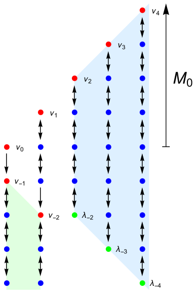
Figure 1: Weight diagram showing the highest (in red) and lowest (in green) weight states under the Lorentz algebra and their descendants (in blue), for the spin 2 case with $\bar{h}-h=2$. An arrow pointing up (down) means that the states are linked by the action of $M_{-1}$ ($M_{1}$). We note that the states $\nu_{-1}$ and $\nu_{-2}$ are null primaries. The states in the blue shaded region are the $V^{(t)}_{a}$ which form an irreducible representation of the full AdS algebra $sl(2,\mathbb{R})\oplus\overline{sl(2,\mathbb{R})}$. Only the states in the green shaded region are actually normalizeable.

Setting $\tilde{k}=2s+k$ in (144), we find that $\nu_{s+k}\sim M_{-1}^{2(s+k)}\lambda_{-s-k}$ and hence these vectors are the lowest and highest weights of a $2(s+k)+1$-dimensional spin-$(s+k)$ representation, denoted as ${\cal D}(s+k)$ in Section 3.2. We will denote the basis vectors in the ${\cal D}(t)$ multiplet as $V^{(t)}_{a}$, with $a$ running from $-t$ to $t$ and normalized as follows:

$$V^{(t)}_{a}=(-1)^{t+a}{(t-a)!\over(2t)!}M_{-1}^{t+a}\left(L_{1}^{t-s}\lambda_{-s}\right),\qquad t\geq s,|a|\leq t$$ (145)

Our normalization constants are chosen such that $V^{(t)}_{-t}=\lambda_{-t},V^{(t)}_{t}=\nu_{t}$ and such that the Lorentz generators act as

$$M_{m}V^{(t)}_{a}=(mt+a)V^{(t)}_{a-m}\,.$$ (146)

For the explicit component expression of the $V^{(t)}_{a}$ one finds

$$V^{(t)}_{a}=\sum_{n\in\mathbb{N}}v_{n}(h,\bar{h};t,a)|n\rangle_{\vphantom{\bar{h}}h}\,{}_{\bar{h}}\langle n-a-s|,\qquad{\rm for\ }h\leq\bar{h}$$ (147)

with (recall $\Delta\equiv h+\bar{h}$)

$$v_{n}(h,\bar{h};t,a)= {(t-a)!\over(2t)!}\sum_{l=0}^{t+a}(-)^{l}\binom{t+a}{l}\Big{(}(1-2h-n)_{l}(-n)_{l}(1-l+n)_{t-s}(2h-l+n)_{t+s}$$

$$(2-a-s+n)_{t+a-l-1}(1+\Delta-a+n)_{t+a-l-1}(1-a-s+n)(\Delta-a+n)\Big{)}^{1/2}\,,$$ (148)

where $(x)_{n}=x(x+1)\dots(x+n-1)$ denotes the Pochhammer symbol. To find similar expressions for the case $h>\bar{h}$, one notes that the Hermitean conjugate $(V^{(t)}_{a})^{\dagger}$ is a state of weight $-a$ in the space $({\cal D}_{+}(\bar{h}),{\cal D}_{-}({h}))$, leading to

$$V^{(t)}_{a}=\sum_{n\in\mathbb{N}}v_{n}(\bar{h},h;t,-a)|n+a-s\rangle_{\vphantom{\bar{h}}h}\,{}_{\bar{h}}\langle n|,\qquad{\rm for\ }h\geq\bar{h}$$ (149)

As we saw in (146), the vectors $V^{(t)}_{a}$ span the representation $\oplus_{t=s}^{\infty}{\cal D}(t)$ under the Lorentz subalgebra generated by $M_{m}$. What is more, they also transform among themselves under the full $sl(2,\mathbb{R})\oplus\overline{sl(2,\mathbb{R})}$ symmetry, under which they form a single irreducible representation. To see this, we have to work out how the AdS translation generators act on them; one can derive the following relation:

$$P_{m}V^{(t)}_{a}=2V^{(t+1)}_{a-m}-{\mu s\over t(t+1)}(mt+a)V^{(t)}_{a-m}+{(s^{2}-t^{2})(\mu^{2}-t^{2})\over 2t(2t+1)}d_{m}(t,a)V^{(t-1)}_{a-m}\,.$$ (150)

where $\mu$ was defined in (71) and we defined the coefficients

$$d_{\pm}(t,a)={(a\pm t)(a\pm(t-1))\over t(2t-1)},\qquad d_{0}(t,a)={a^{2}-t^{2}\over t(2t-1)}\,.$$ (151)

The coefficients in (150) are completely fixed by the properties (141,142), consistency with the AdS algebra (119) and the Casimir relation

$$\eta^{mn}P_{m}P_{n}V^{(t)}_{a}=\left(2h(h-1)+2\bar{h}(\bar{h}-1)-t(t+1)\right)V^{(t)}_{a}\,.$$ (152)

We also verified (150) using the explicit expressions (147).

We also mention a further useful relation involving the action of the translation generators $P_{m}$ on the vectors $V^{(t)}_{a}$. Recalling that these act as $P_{m}\psi=L_{m}\psi+\psi L_{m}$ one can derive the following identity

$$M_{-1}^{n+1}P_{1}=n(n+1)P_{-1}M_{-1}^{n-1}-2(n+1)P_{0}M_{-1}^{n}+P_{1}M_{-1}^{n+1}\,.$$ (153)

Combining this with (145), we find a relation expressing the vectors in the spin-$t+1$ representation in terms of the action of the translation generators on vectors in the spin-$t$ representation:

$$V^{(t+1)}_{a}=\sum_{m=-1}^{1}c_{m}(t,a)P_{m}V^{(t)}_{a+m}$$ (154)

where

$$c_{-1}={(t+a)(t+a+1)\over 2(2t+2)(2t+1)},\qquad c_{0}={(t+a+1)(t-a+1)\over(2t+2)(2t+1)},\qquad c_{1}={(t-a+1)(t-a)\over 2(2t+2)(2t+1)}\,.$$ (155)

In (144) we also found, for $\bar{h}>h$, a number of highest weight vectors, namely $\nu_{-s+\tilde{k}}$ for $0\leq\tilde{k}<2s$, for which there is no corresponding lowest weight vector and which hence do not fit in finite-dimensional representations. Though these do not play a role in the present work (see however the Outlook section), we now briefly comment on the Lorentz representations carried by these states. One checks that $\nu_{-s+\tilde{k}}$ for $0\leq\tilde{k}<s-{1\over 2}$ is actually a Lorentz descendant of $\nu_{s-\tilde{k}-1}$:

$$\nu_{-s+\tilde{k}}\sim M_{1}^{2(s-\tilde{k})-1}\nu_{s-\tilde{k}-1}\qquad{\rm for\ }0\leq k<s-{1\over 2}\,.$$ (156)

The $\nu_{-s+\tilde{k}}$ for $0\leq\tilde{k}<s-{1\over 2}$ and their descendants therefore form an invariant subspace whose complement is not invariant; in that case $\nu_{-s+\tilde{k}}$ and $\nu_{s-\tilde{k}-1}$ belong to an infinite-dimensional reducible but indecomposable representation of the Lorentz subalgebra.

Let us also discuss the normalizablility of the vectors constructed above with respect to the inner product (80). One finds that the norm of the highest weight vectors for $\bar{h}\geq h$ is

$$|\nu_{-s+\tilde{k}}|^{2}={k!(2h+\tilde{k}-1)!\over(2\bar{h}-1)!}\,_{2}F_{1}(\tilde{k}+1,2h+\tilde{k},2\bar{h},1),\qquad{\rm for\ }h\leq\bar{h}$$ (157)

Using well-known convergence properties of the hypergeometric function abramowitz , we find that the highest weight states are therefore normalizable for $\tilde{k}<s-{1\over 2}$. In other words, only the ‘null’ highest weight vectors discussed above are actually normalizeable. In particular, the vectors $V^{(t)}_{a}$ comprising the finite-dimensional representations are not normalizable.

References

- (1) M. Fierz and W. Pauli, “On relativistic wave equations for particles of arbitrary spin in an electromagnetic field,” Proc. Roy. Soc. Lond. A 173, 211 (1939).
- (2) R. Rahman and M. Taronna, “From Higher Spins to Strings: A Primer,” arXiv:1512.07932 [hep-th].
- (3) X. Bekaert, S. Cnockaert, C. Iazeolla and M. A. Vasiliev, “Nonlinear higher spin theories in various dimensions,” hep-th/0503128.
- (4) V. E. Didenko and E. D. Skvortsov, “Elements of Vasiliev Theory,” hep-th/1401.2975.
- (5) E. S. Fradkin and M. A. Vasiliev, “On the Gravitational Interaction of Massless Higher Spin Fields,” Phys. Lett. B 189, 89 (1987).
- (6) V. E. Lopatin and M. A. Vasiliev, “Free Massless Bosonic Fields of Arbitrary Spin in -dimensional De Sitter Space,” Mod. Phys. Lett. A 3, 257 (1988).
- (7) M. A. Vasiliev, “Free Massless Fermionic Fields of Arbitrary Spin in -dimensional De Sitter Space,” Nucl. Phys. B 301, 26 (1988).
- (8) M. A. Vasiliev, “Equations of Motion of Interacting Massless Fields of All Spins as a Free Differential Algebra,” Phys. Lett. B 209, 491 (1988).
- (9) M. A. Vasiliev, “Unfolded representation for relativistic equations in (2+1) anti-De Sitter space,” Class. Quant. Grav. 11, 649 (1994).
- (10) A. V. Barabanshchikov, S. F. Prokushkin and M. A. Vasiliev, “Free equations for massive matter fields in (2+1)-dimensional anti-de Sitter space from deformed oscillator algebra,” Teor. Mat. Fiz. 110N3, 372 (1997) [Theor. Math. Phys. 110, 295 (1997)] [hep-th/9609034].
- (11) C. Iazeolla and P. Sundell, “A Fiber Approach to Harmonic Analysis of Unfolded Higher-Spin Field Equations,” JHEP 0810, 022 (2008) [arXiv:0806.1942 [hep-th]].
- (12) N. Boulanger, C. Iazeolla and P. Sundell, “Unfolding Mixed-Symmetry Fields in AdS and the BMV Conjecture: I. General Formalism,” JHEP 0907, 013 (2009) [arXiv:0812.3615 [hep-th]].
- (13) N. Boulanger, C. Iazeolla and P. Sundell, “Unfolding Mixed-Symmetry Fields in AdS and the BMV Conjecture. II. Oscillator Realization,” JHEP 0907, 014 (2009) [arXiv:0812.4438 [hep-th]].
- (14) D. S. Ponomarev and M. A. Vasiliev, “Frame-Like Action and Unfolded Formulation for Massive Higher-Spin Fields,” Nucl. Phys. B 839, 466 (2010) [arXiv:1001.0062 [hep-th]].
- (15) N. Boulanger, D. Ponomarev, E. Sezgin and P. Sundell, “New unfolded higher spin systems in ,” Class. Quant. Grav. 32, no. 15, 155002 (2015) [arXiv:1412.8209 [hep-th]].
- (16) Y. M. Zinoviev, “Massive higher spins in d = 3 unfolded,” J. Phys. A 49, no. 9, 095401 (2016) [arXiv:1509.00968 [hep-th]].
- (17) I. L. Buchbinder, T. V. Snegirev and Y. M. Zinoviev, “Unfolded equations for massive higher spin supermultiplets in AdS3,” JHEP 1608, 075 (2016) [arXiv:1606.02475 [hep-th]].
- (18) M. A. Vasiliev, “Consistent equation for interacting gauge fields of all spins in (3+1)-dimensions,” Phys. Lett. B 243, 378 (1990).
- (19) S. F. Prokushkin and M. A. Vasiliev, “Higher spin gauge interactions for massive matter fields in 3-D AdS space-time,” Nucl. Phys. B 545, 385 (1999) [hep-th/9806236].
- (20) M. R. Gaberdiel and R. Gopakumar, “An AdS3 Dual for Minimal Model CFTs,” Phys. Rev. D 83, 066007 (2011) [arXiv:1011.2986 [hep-th]].
- (21) M. R. Gaberdiel and R. Gopakumar, “Higher Spins & Strings,” JHEP 1411, 044 (2014) [arXiv:1406.6103 [hep-th]].
- (22) M. R. Gaberdiel and R. Gopakumar, “Stringy Symmetries and the Higher Spin Square,” J. Phys. A 48, no. 18, 185402 (2015) [arXiv:1501.07236 [hep-th]].
- (23) M. R. Gaberdiel and R. Gopakumar, “String Theory as a Higher Spin Theory,” JHEP 1609, 085 (2016) [arXiv:1512.07237 [hep-th]].
- (24) G. Giribet, C. Hull, M. Kleban, M. Porrati and E. Rabinovici, “Superstrings on AdS3 at ,” arXiv:1803.04420 [hep-th].
- (25) M. R. Gaberdiel and R. Gopakumar, “Tensionless String Spectra on ,” arXiv:1803.04423 [hep-th].
- (26) J. Raeymaekers, “On matter coupled to the higher spin square,” J. Phys. A 49, no. 35, 355402 (2016) [arXiv:1603.07845 [hep-th]].
- (27) L. Castellani, R. D’Auria and P. Fre, “Supergravity and superstrings: A Geometric perspective. Vol. 1: Mathematical foundations,” Singapore, Singapore: World Scientific (1991) 1-603
- (28) E. Witten, “(2+1)-Dimensional Gravity as an Exactly Soluble System,” Nucl. Phys. B 311, 46 (1988).
- (29) V. Balasubramanian, P. Kraus and A. E. Lawrence, “Bulk versus boundary dynamics in anti-de Sitter space-time,” Phys. Rev. D 59, 046003 (1999) [hep-th/9805171].
- (30) A. Kitaev, “Notes on representations,” arXiv:1711.08169 [hep-th].
- (31) S. Deser, R. Jackiw and S. Templeton, “Topologically Massive Gauge Theories,” Annals Phys. 140, 372 (1982) [Annals Phys. 281, 409 (2000)] Erratum: [Annals Phys. 185, 406 (1988)].
- (32) I. V. Tyutin and M. A. Vasiliev, “Lagrangian formulation of irreducible massive fields of arbitrary spin in (2+1)-dimensions,” Teor. Mat. Fiz. 113N1, 45 (1997) [Theor. Math. Phys. 113, 1244 (1997)] [hep-th/9704132].
- (33) E. A. Bergshoeff, O. Hohm and P. K. Townsend, “On Higher Derivatives in 3D Gravity and Higher Spin Gauge Theories,” Annals Phys. 325, 1118 (2010) [arXiv:0911.3061 [hep-th]].
- (34) S. Deger, A. Kaya, E. Sezgin and P. Sundell, “Spectrum of D = 6, N=4b supergravity on AdS in three-dimensions x S**3,” Nucl. Phys. B 536, 110 (1998) [hep-th/9804166].
- (35) J. Repka, “Tensor products of unitary representations of ,” Bull. Amer. Math. Soc. 82, 930 (1976).
- (36) T. Ortin, “A Note on Lie-Lorentz derivatives,” Class. Quant. Grav. 19, L143 (2002) [hep-th/0206159].
- (37) C. N. Pope, L. J. Romans and X. Shen, “(infinity) and the Racah-wigner Algebra,” Nucl. Phys. B 339, 191 (1990).
- (38) M. Ammon, P. Kraus and E. Perlmutter, “Scalar fields and three-point functions in D=3 higher spin gravity,” JHEP 1207, 113 (2012) [arXiv:1111.3926 [hep-th]].
- (39) A. Campoleoni, T. Prochazka and J. Raeymaekers, “A note on conical solutions in 3D Vasiliev theory,” JHEP 1305, 052 (2013) [arXiv:1303.0880 [hep-th]].
- (40) P. Kessel and J. Raeymaekers, work in progress.
- (41) M. A. Vasiliev, “Current Interactions and Holography from the 0-Form Sector of Nonlinear Higher-Spin Equations,” JHEP 1710, 111 (2017) [arXiv:1605.02662 [hep-th]].
- (42) M. Abramowitz and I.A. Stegun “Handbook of Mathematical Functions,” Dover (1972)