Shielding effects in random large area field emitters, the field enhancement factor distribution and current calculation

Abstract

A finite-size uniform random distribution of vertically aligned field emitters on a planar surface is studied under the assumption that the asymptotic field is uniform and parallel to the emitter axis. A formula for field enhancement factor is first derived for a 2-emitter system and this is then generalized for $N$-emitters placed arbitrarily (line, array or random). It is found that geometric effects dominate the shielding of field lines. The distribution of field enhancement factor for a uniform random distribution of emitter locations is found to be closely approximated by an extreme value (Gumbel-minimum) distribution when the mean separation is greater than the emitter height but is better approximated by a Gaussian for mean separations close to the emitter height. It is shown that these distributions can be used to accurately predict the current emitted from a large area field emitter.

I Introduction

The in-principle advantages of using field emission cathodes over thermionic ones are manifold. Issues associated with high temperature operation and temporal response in thermionic cathodes clearly indicate that next-generation high performance electron emission systems for use in vacuum devices must be based on field emission teo ; parmee . The strides achieved in the past decades in our ability to pattern arrays of pointed emitters spindt68 ; spindt76 ; spindt91 and the discovery of carbon nanotubes (CNT) as a suitable material deHeer ; cole2014 for stable operation, have led to vigorous research activity in this direction. These efforts are supported by theoretical studies on large area field emitters (LAFE) zhbanov ; forbes2012 ; read_bowring ; harris15 ; forbes2016 ; jensen_ency ; jap2016 and corrections for nano-tipped emitters jensen_image ; db_imag ; db_ext to the planar Fowler-Nordheim (FN) formula for current density FN ; murphy ; forbes ; forbes_deane . Despite this progress, there are several challenges in our ability to predict theoretically, the current emitted by a single emitter or a cluster of emitters placed randomly or in an array.

The Fowler-Nordheim formalism continues to remain relevant despite the vast change in experimental field-emission setups. This is surprising considering that it is based on a planar model for metallic emitters. Field emitters of today are highly curved leading to large local electric fields at the apex due to the phenomenon known as field-enhancement. Thus, moderate asymptotic fields ($\sim$ V/$\mu$m) can lead to local fields as large as 5-10 V/nm, at which appreciable field emission can occur. The transition from planar to curved emitters in field-emission theory is generally made using a local apex field enhancement factor (AFEF) $\gamma_{a}$ forbes2003 ; db_fef . It does not change the shape of traditional FN-plots and allows one to extract the parameter $\gamma_{a}$. However, theoretical estimates of the emission current require knowledge about the AFEF and efforts in this direction depend either on analytically tractable models such as the hemisphere or hemiellipsoid on a plane in the presence of an asymptotic field $E_{0}$ that is uniform and parallel to the emitter axis or rely on finite-element codes for particular emitter shapes and diode configuration. Using a different approach, a recent study using the line charge model (LCM), generalizes the known result for the hemiellipsoid and expresses the apex field enhancement factor as

$$\gamma_{a}=\frac{2h/R_{a}}{\alpha_{1}\ln(4h/R_{a})-\alpha_{2}}$$ (1)

where $h$ is the height of the emitter, $R_{a}$ the apex radius of curvature and $\alpha_{1},\alpha_{2}$ depend on the details of the line charge and hence the emitter shape. It was also found numerically that the field enhancement factor is equally well described by the simpler form

$$\gamma_{a}=\frac{2h/R_{a}}{\ln(4h/R_{a})-\alpha_{0}}$$ (2)

where $\alpha_{0}$ was found to depend on the emitter base (e.g. cone, ellipsoid, cylinder). Single emitter predictions for emitter current can thus be made under the condition that the image charges at the anode can be neglected (large anode-cathode separation) and the work function and band-structure variations on the active emission surface is negligible db2018_pop1 ; db_fef .

While single emitter setups are important in their own right, an efficient and bright electron source requires a large area field emitter comprising of numerous emission tips (such as CNTs) placed in an array or even randomly. From a theoretical perspective, despite all simplifying assumptions, there is the added complication of each emitting site in a finite-sized patch, having a different enhancement factor due to the process of shielding. Emitters in close proximity “shield” an emitter apex thereby lowering the enhancement factor from its un-shielded value. While attempts have been made to understand the shielding process using models such as the floating-sphere on emitter plane potential as well as numerically, a quick and accurate prediction of the apex field enhancement factors in a LAFE based on the proximity of the other emitters, or even an estimate of the average enhancement factor for a given mean separation, is not available.

We shall deal here with a cluster of emitters, all having the same height and apex radius of curvature but placed randomly following a uniform distribution on a rectangular patch. Our methods allow us to deal with arrays as well. Our interest is twofold. First, we shall try to understand the process of shielding and try to arrive at a simple unifying picture. Next, we shall probe the existence of a universal field enhancement factor distribution groening2001 ; cole2014 ; groening2015 when the emitters are placed randomly. This is then used to find the net emission current from a random LAFE. Our approach here is a generalization of the method adopted recently db_fef to arrive at Eq. 1. We shall first introduce the line charge model and consider the case of two emitters. The result can then easily be generalized to $N$-emitters.

II The 2-Emitter case - line charge model

Consider two emitters of height $h$, apex radius of curvature $R_{a}$, separated by a distance $\rho_{12}$, placed on a grounded metallic plane and aligned along an asymptotic (away from the emitter tips) electrostatic field $-E_{0}\hat{z}$. If we assume the first emitter to be centred at the origin such that its apex has co-ordinates $(\rho,z)=(0,h)$ while the apex of the second emitter is located at $(\rho,z)=(\rho_{12},h)$. This setup can be modelled by 2 vertical line charge distributions and their image. Since the emitters are identical in every other respect, they possess identical line charge density $\Lambda(z)$ of extent $L$. We shall assume that the line charge density is linear: $\Lambda(z)=\lambda z$. This puts a restriction on the shape of each emitter-base but otherwise does not pose any limitation on the main conclusions regarding shielding. Thus, in view of the linearity assumption, we are considering two ellipsoid-like emitters placed a distance $\rho_{12}$ apart. The potential at any point ($\rho,z$) can be expressed as db_fef

$$\begin{split}V(\rho,z)=&\frac{1}{4\pi\epsilon_{0}}\Big{[}\int_{-L}^{L}\frac{\lambda s}{\big{[}\rho^{2}+(z-s)^{2}\big{]}^{1/2}}ds~{}+\\ &\int_{-L}^{L}\frac{\lambda s}{\big{[}(\rho-\rho_{12})^{2}+(z-s)^{2}\big{]}^{1/2}}ds\Big{]}+E_{0}z\end{split}$$ (3)

where the integration is along the $z-$axis from $[-L,L]$, $L$ being the extent of the line charge distribution along the $z-$axis and $E_{0}$ is the magnitude of the asymptotic field or the external field in the absence of the ellipsoidal protrusion. The parameter $\lambda$ can be fixed by demanding that potential vanishes at the apex. Thus, at the apex of either emitter,

$$\begin{split}\frac{\lambda}{4\pi\epsilon_{0}}\Big{[}&\int_{-L}^{L}\frac{s}{\big{[}(\rho_{12})^{2}+(h-s)^{2}\big{]}^{1/2}}ds~{}+\\ &\int_{-L}^{L}\frac{s}{(h-s)}ds\Big{]}~{}+~{}E_{0}h=0.\end{split}$$ (4)

When the two emitters are well separated, the zero-potential contour of the above potential defines 2 ellipsoidal emitters, each with base radius $b=(h^{2}-L^{2})^{1/2}$ and separated by $\rho_{12}$, mounted on a flat planar surface. As the emitters are brought closer, the zero potential contour keeps the apex invariant due to the imposition of Eq. 4, but its shape deviates slightly from an ellipsoid as it approaches the base. The effect gets especially marked when the separation is small ($\rho_{12}/h<0.2$) and the linear line charge density can no longer be used to model the 2-emitter ellipsoidal system. We shall therefore steer clear of this regime. Furthermore, we shall assume that the deviation in the zero-potential contour of individual emitters away from the apex, introduces a change in the apex field enhancement factor that is small compared to the direct effect of neighbouring emitters at the apex. Note that for an isolated emitter, the parameter $L=\sqrt{h(h-R_{a})}$ db_fef . Since the imposition of Eq. 4 preserves the height and apex radius of curvature of the zero-potential surface, this quantity remains invariant for $\rho_{12}/h>0.2$.

We are interested here in the field enhancement factor, $\gamma_{a}$. For axially symmetric emitters aligned along $\hat{z}$, this is defined as $\gamma_{a}=-\frac{1}{E_{0}}\frac{\partial V}{\partial z}{|_{\rho=0,z=h}}$. Our starting point for the AFEF is Eq. 3. At the apex, $(\rho,z)=(0,h)$ of emitter 1,

$$\begin{split}\frac{\partial V}{\partial z}{|_{(\rho=0,z=h)}}=&-\frac{\lambda}{4\pi\epsilon_{0}}\Big{[}\int_{-L}^{L}\frac{s}{(h-s)^{2}}ds~{}+\\ &\int_{-L}^{L}\frac{s(h-s)}{\big{[}\rho_{12}^{2}+(h-s)^{2}\big{]}^{3/2}}ds\Big{]}+E_{0}\end{split}$$ (5)

which, on integrating, leads to

$$\begin{split}\frac{\partial V}{\partial z}{|_{(\rho=0,z=h)}}=&-\frac{\lambda}{4\pi\epsilon_{0}}\Big{[}\frac{2hL}{h^{2}-L^{2}}+\ln\Big{(}\frac{h+L}{h-L}\Big{)}\\ &+\int_{-L}^{L}\frac{s(h-s)}{\big{[}\rho_{12}^{2}+(h-s)^{2}\big{]}^{3/2}}ds\Big{]}+E_{0}.\end{split}$$ (6)

For $\rho_{12}$ large compared to the base radius of the emitters, the integral in Eq. 6 is negligible compared to the first two terms in the square bracket. Furthermore, for sharp emitters ($h/R_{a}>>1$), only the first term dominates db_fef . Thus

$$\frac{\partial V}{\partial z}{|_{(\rho=0,z=h)}}=-\frac{\lambda}{4\pi\epsilon_{0}}\Big{[}\frac{2hL}{h^{2}-L^{2}}\Big{]}.$$ (7)

It now remains to determine $\lambda$ using Eq. 4. The integrals in Eq. 4 yield

$$\begin{split}\frac{\lambda}{4\pi\epsilon_{0}}\Big{[}&-\int_{-L}^{L}\frac{h-s}{\big{[}(\rho_{12})^{2}+(h-s)^{2}\big{]}^{1/2}}ds~{}+\\ &h\int_{-L}^{L}\frac{ds}{\big{[}(\rho_{12})^{2}+(h-s)^{2}\big{]}^{1/2}}+\\ &h\ln\Big{(}\frac{h+L}{h-L}\Big{)}-2L\Big{]}+E_{0}h=0\end{split}$$ (8)

which further simplifies as

$$\begin{split}\frac{\lambda}{4\pi\epsilon_{0}}\Bigg{[}&\Big{[}\sqrt{\rho_{12}^{2}+(h-s)^{2}}~{}+\\ &h\ln\Big{|}\sqrt{1+\frac{(h+s)^{2}}{\rho_{12}^{2}}}+\frac{(h+s)}{\rho_{12}}\Big{|}~{}\Big{]}_{-L}^{L}+\\ &h\ln\Big{(}\frac{h+L}{h-L}\Big{)}-2L\Bigg{]}+E_{0}h=0.\end{split}$$ (9)

Note that

$$\sqrt{\rho_{12}^{2}+(h-s)^{2}}\Big{|}_{-L}^{L}\simeq\rho_{12}\Big{[}1-\big{(}1+4\delta_{12}^{2}\big{)}^{1/2}\Big{]}$$ (10)

where $\delta_{12}=h/\rho_{12}$. Also,

$$\ln\Bigg{|}\sqrt{1+\frac{(h+s)^{2}}{\rho_{12}^{2}}}+\frac{(h+s)}{\rho_{12}}\Bigg{|}_{-L}^{L}\simeq\ln\Big{|}\sqrt{1+4\delta_{12}^{2}}+2\delta_{12}\Big{|}$$ (11)

if $\rho_{12}>>b$. Finally, using $h\simeq L$ for nano-tipped emitters, we have

$$\lambda=-\frac{4\pi\epsilon_{0}E_{0}}{\ln\frac{4h^{2}}{h^{2}-L^{2}}-2+\alpha_{S_{12}}}$$ (12)

where the shielding term

$$\alpha_{S_{12}}=\frac{1}{\delta_{12}}\Big{[}1-\sqrt{1+4\delta_{12}^{2}}\Big{]}+\ln\Big{|}\sqrt{1+4\delta_{12}^{2}}+2\delta_{12}\Big{|}$$ (13)

Thus

$$\gamma_{a}=\frac{2h/R_{a}}{\ln\big{(}4h/R_{a}\big{)}-2+\alpha_{S_{12}}}$$ (14)

is the enhancement factor of the 2-emitter system.

A topic of recent interest has been the change in 2-emitter AFEF as compared to the single or un-shielded case ($\gamma_{a}^{(1)}$). Note that for the isolated or single case, $\alpha_{S_{12}}=0$ so that the relative change

$$\frac{\gamma_{a}-\gamma_{a}^{(1)}}{\gamma_{a}^{(1)}}=-\frac{\alpha_{S_{12}}}{\Delta}$$ (15)

where $\Delta=\ln\big{(}4h/R_{a}\big{)}-2$. For large separations ($\rho_{12}$ large), $\delta_{12}$ is small and it is easy to verify that the

$$\alpha_{S_{12}}=\frac{2}{3}\delta_{12}^{3}+{\cal{O}}(\delta_{12}^{5}).$$ (16)

Thus, at large separations,

$$\frac{\gamma_{a}-\gamma_{a}^{(1)}}{\gamma_{a}^{(1)}}\sim\frac{1}{\rho_{12}^{3}}$$ (17)

as deduced by other methods forbes2018 ; agnol2018 .

II.1 The N-emitter case

The 2-emitter case was simple in that everything else being equal, both emitters have the same line charge density. As a consequence, the shielding term $\alpha_{S_{12}}$ does not depend on $\lambda_{1,2}$. For a N-emitter system, $N\geq 3$, the line charge densities are unequal since different emitters have different degrees of shielding. The mutual shielding term thus generalizes as

$$\tilde{\alpha}_{S_{ij}} = \frac{\lambda_{j}}{\lambda_{i}}\alpha_{S_{ij}},~{}\text{where}$$ (18)

$$\alpha_{S_{ij}} = \frac{1}{\delta_{12}}\Big{[}1-\sqrt{1+4\delta_{ij}^{2}}\Big{]}+\ln\Big{|}\sqrt{1+4\delta_{ij}^{2}}+2\delta_{ij}\Big{|}$$

and $\lambda_{j}/\lambda_{i}\neq 1$ in general. The net shielding due to N-emitters can be expressed as

$$\tilde{\alpha}_{S_{i}}=\sum_{j\neq i}{\tilde{\alpha}}_{S_{ij}}.$$ (19)

This follows on noting that Eq. 7 can be expressed for the $i^{th}$ emitter apex located at ($\rho_{i},h$) with respect to an arbitrary origin, as

$$\frac{\partial V}{\partial z}{|_{(\rho=\rho_{i},z=h)}}\simeq-\frac{\lambda_{i}}{4\pi\epsilon_{0}}\Big{[}\frac{2hL}{h^{2}-L^{2}}\Big{]}$$ (20)

since the other terms are small and can be neglected as before. Further, Eq. 4 can be expressed as

$$\begin{split}\frac{\lambda_{i}}{4\pi\epsilon_{0}}\Big{[}&\sum_{j\neq i}\frac{\lambda_{j}}{\lambda_{i}}\int_{-L}^{L}\frac{s}{\big{[}(\rho_{12})^{2}+(h-s)^{2}\big{]}^{1/2}}ds~{}+\\ &\int_{-L}^{L}\frac{s}{(h-s)}ds\Big{]}~{}+~{}E_{0}h=0\end{split}$$ (21)

so that {$\lambda_{i}$} can be determined by simultaneously solving the set of $N$ equations. We shall instead merely express $\lambda_{i}$ in terms of the ratio $\lambda_{j}/\lambda_{i}$ and use it in Eq. 20 to express the field enhancement factor

$$\gamma_{a}^{(i)} = \frac{2h/R_{a}}{\ln\big{(}4h/R_{a}\big{)}-2+\sum_{j\neq i}\frac{\lambda_{j}}{\lambda_{i}}\alpha_{S_{ij}}}$$ (22)

$$= \frac{2h/R_{a}}{\ln\big{(}4h/R_{a}\big{)}-2+\tilde{\alpha}_{S_{i}}}$$ (23)

for the $i^{th}$ emitter.

Eq. 23 as such does not help us in computing $\gamma_{a}^{(i)}$ without actually solving the electrostatic problem. However, there are clearly two aspects in the shielding term that must draw our attention. The first is a geometric factor $\alpha_{S_{ij}}$ which merely depends on the ratio of the height $h$ and the mutual distance $\rho_{ij}$ and does not require a solution of the Poisson equation. The second is the ratio $\lambda_{j}/\lambda_{i}$ which does require knowledge about the line charge density. As a first approximation, for average separations $\rho_{ij}$ comparable to or larger than the height $h$, we set the ratio $\lambda_{j}/\lambda_{i}=1$. Thus $\tilde{\alpha}_{S_{i}}=\alpha_{S_{i}}$ so that

$$\gamma_{a}^{(i)} \simeq \frac{2h/R_{a}}{\ln\big{(}4h/R_{a}\big{)}-2+\sum_{j\neq i}\alpha_{S_{ij}}}$$ (24)

$$= \frac{2h/R_{a}}{\ln\big{(}4h/R_{a}\big{)}-2+\alpha}_{S_{i}}.$$ (25)

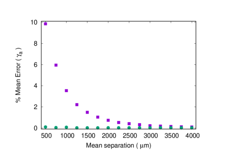
Figure 1: The mean error in apex field enhancement factor (AFEF) is shown for different mean spacings. A total of 2500 emitters is considered in each case. The field enhancement factor is computed using Eq. 23 (denoted by $\CIRCLE$), and, Eq. 25 (denoted by $\blacksquare$). The error in the second case decreases as the mean spacing exceeds the height $h=1500~{}\mu m$. The emitters have a base radius $b=10~{}\mu$m and an apex radius $R_{a}=66.67~{}$nm. For Eq. 23, the error is uniformly small ($\leq 0.05\%$).

A comparison of the discrepancy between the AFEF values computed using Eq. 23 and 25 is shown in Fig. 1 for a randomly distributed N-emitter system. The emitters positions are drawn from a uniform distribution using a standard random number generator. It is apparent that the error on ignoring the variation in $\{\lambda_{i}\}$ is acceptable when the mean separation exceeds the emitter height. Moreover even when the separation is half the emitter height, the average error is only $6\%$. Thus, the shielding process is pre-dominantly a geometric effect and the field enhancement factor can be computed quite accurately only from a knowledge of the positions, height and apex radius of curvature of the emitters. We have also determined the mean error of only those emitters for which the AFEF exceeds the mean value of the AFEF since these predominantly contribute to the field-emission current at low to medium local field strengths ($<7$V/nm). The mean error for both Eq. 23 and Eq. 25 is then as small as 0.02% at all spacings considered. Thus, Eq. 25 can be used to accurately determine the field enhancement factor in a uniform random distribution of field-emitters.

III The field-enhancement-factor distribution for randomly placed emitters

As seen above, the field enhancement factor can be computed for individual emitters in a LAFE purely from geometrical considerations. While this information is useful, a distribution of field enhancement factors is desirable so that the total current emitted from a LAFE can be computed based on only a few parameters such as the mean and standard deviation of the AFEF distribution. We shall thus explore the existence of a universal AFEF distribution when the emitters are distributed uniformly on a rectangular patch.

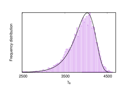
Figure 2: The normalized frequency distribution of the field enhancement factors together with the Gumbel (minimum) distribution (solid curve). The LAFE has a mean separation $2000~{}\mu$m containing 5000 emitters, each of height $h=1500~{}\mu$ m. The parameters of the Gumbel distribution are fixed using Eqns. 28 and 29 with the mean $\mu$ and standard deviation $\sigma$ calculated using the exact numerical values of AFEF which are obtained by numerical differentiation of the potential.

Our studies on the field-enhancement-factor distribution for various mean separations, height and apex radius show that the distribution is closer to a Gaussian when the mean separation is equal to or somewhat smaller than the emitter height. However, as the mean separation increases, the field-enhancement-factor distribution is skewed to the left for emitters distributed uniformly on a rectangular patch as seen in Fig. 2. The skewness persists for separations beyond twice the emitter height. Also, its mean and standard deviation depend on the mean separation of emitters. While the mean AFEF increases with separation, the standard deviation decreases.

An analytical expression for the AFEF distribution is difficult to derive but fits to various left-skewed distributions show that the Gumbel minimum distribution best describes the field enhancement factor for mean separations exceeding the emitter height. This is also the region of interest since as the optimal separation at which the current density is highest lies here.

The Gumbel distribution has a probability density function

$$f_{\gamma}(x)=\frac{1}{\beta}e^{\frac{x-\alpha}{\beta}}e^{-e^{\frac{x-\alpha}{\beta}}}$$ (26)

and its cumulative density function is

$$F_{\gamma}(x)=1-e^{-e^{\frac{x-\alpha}{\beta}}}.$$ (27)

Here $\alpha$ and $\beta$ are parameters in terms of which, the mean $\mu$ and standard deviation $\sigma$ are

$$\mu = \alpha-\beta\gamma_{EM}$$ (28)

$$\sigma = \pi\beta/\sqrt{6}$$ (29)

where $\gamma_{EM}\simeq 0.5772$ is the Euler-Mascheroni constant. Using the numerically calculated values of apex field enhancement factor $\gamma_{a}$, $\mu$ and $\sigma$ can be determined. The Gumbel parameters $\alpha$ and $\beta$ can thus be evaluated using Eqns. 28 and 29. A comparison of the normalized frequency distribution with the Gumbel distribution is shown in Fig. 2. The agreement is good for mean separations exceeding the emitter height.

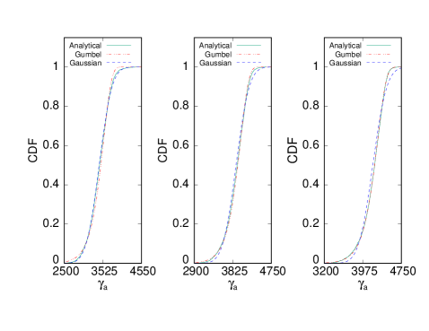
Figure 3: A comparison of the cumulative density function (CDF) with the Gaussian and Gumbel minimum distributions for 3 values of mean separation. The values of $\gamma_{a}$ are obtained using the analytical expression Eq. 25. The mean separations are $1500~{}\mu$m (left), $2000~{}\mu$m (middle) and $2500~{}\mu$m (right) while the height of the emitters is $1500~{}\mu$m. The parameters for the Gaussian and Gumbel distributions are obtained using the mean and standard deviation.

The Gumbel distribution thus shows good agreement when the AFEF values are determined by numerical differentiation after solving for the electrostatic potential (Eq. 23 may instead be used since the errors are small at all separations but requires knowledge of the line charge density). We can alternately study the AFEF distribution when individual AFEF values are determined using Eq. 25 which does not require knowledge of the electrostatic problem. The Gumbel distribution again provides a good approximation when the mean separation between emitters exceeds the emitter height (see Fig. 3) while the Gaussian distribution is a better approximation for mean separation around the emitter height. These conclusions hold for other height and apex radius combinations.

III.1 The harmonic mean and standard deviation using the pair-wise distance distribution

So far, we have determined the Gumbel parameters by first computing $\gamma_{a}$ (using Eq. 23 or 25) and determining $\mu$ and $\sigma$. In principle, it should be possible to determine the mean and standard deviation using Eq. 25 (but without evaluating individual $\gamma_{a}^{(i)}$) and noting that the emitters are distributed uniformly. It thus requires knowledge of the probability density function (PDF) of the distance $\rho_{ij}$ where the $i^{th}$ emitter is fixed and the other $N-1$ emitters distributed uniformly in a rectangular patch. The PDF obviously depends on the location of the $i^{th}$ emitter and hence various cases need to be listed. A simpler and well known PDF is that of the pair-wise distance between any 2 points $i$ and $j$ located on a rectangular patch. This can be used to calculate the harmonic mean by noting that Eq. 24 can be rewritten as

$$\frac{2h}{R_{a}}\frac{1}{\gamma_{i}}=\ln\Big{(}\frac{4h}{R_{a}}\Big{)}-2+\sum_{j\neq i}\alpha_{S_{ij}}$$ (30)

so that

$$\frac{2h}{R_{a}}\sum_{i}\frac{1}{\gamma_{i}}=N\Big{[}\ln\Big{(}\frac{4h}{R_{a}}\Big{)}-2\Big{]}+\sum_{i}\sum_{j\neq i}\alpha_{S_{ij}}.$$ (31)

Thus, the harmonic mean, $\mu_{h}$ is

$$\Big{(}\frac{1}{N} \sum\limits_{i} \frac{1}{\gamma_{i}}\Big{)}^{-1}=\frac{\frac{2h}{R_{a}}}{\ln(\frac{4h}{R_{a}})-2+\frac{1}{N}\sum\limits_{i}\sum\limits_{j\neq i}\alpha_{S_{ij}}}$$ (32)

$$= \frac{\frac{2h}{R_{a}}}{\ln(\frac{4h}{R_{a}})-2+(N-1)\int f_{\rho}(x)\alpha_{S}(x)}$$ (33)

where

$$\alpha_{S}(x)=\frac{x}{h}\Big{[}1-\sqrt{1+4\Big{(}\frac{h}{x}\Big{)}^{2}}\Big{]}+\ln\Big{|}\sqrt{1+4\Big{(}\frac{h}{x}\Big{)}^{2}}+2\frac{h}{x}\Big{|}$$ (34)

and the probability density function, $f_{\rho}(x)$, for the pair-wise distance between any two points distributed uniformly on a square patch of length $L$ is related to

$$f_{S}(s)=\begin{cases}-4\frac{\sqrt{s}}{L^{3}}+\frac{\pi}{L^{2}}+\frac{s}{L^{4}}&\text{$0<s\leq L^{2}$;}\\ ~{}~{}~{}~{}~{}\\ -2\frac{1}{L^{2}}+\frac{4}{L^{2}}\sin^{-1}\big{(}\frac{L}{\sqrt{s}}\big{)}+\\ \frac{4}{L^{3}}\sqrt{s-L^{2}}-\frac{\pi}{L^{2}}-\frac{s}{L^{4}}&\text{$L^{2}<s\leq 2L^{2}$}\end{cases}$$ (35)

where $s=x^{2}$ and $f_{\rho}(x)=2xf_{S}(s)$. Note that $\int f_{\rho}(x)dx=1$ so that Eq. 33 has the factor $(N-1)$ multiplying the integral. Thus, the harmonic mean can be evaluated, at least numerically for randomly placed ellipsoidal emitters on a square (see Philip philip for an expression for $f_{S}(s)$ when the area is rectangular) patch.

A similar expression can be derived for

$$\mu_{h2}=\Big{(}\frac{1}{N}\sum_{i}\frac{1}{\gamma_{i}^{2}}\Big{)}^{-1}$$ (36)

using the probability density function $f_{\rho}(x)$ and hence the ‘harmonic’ standard deviation, defined as

$$\sigma_{h}=\Big{[}\Big{(}\frac{1}{N}\sum_{i}\frac{1}{\gamma_{i}^{2}}\Big{)}^{-1}-\Big{(}\frac{1}{N}\sum_{i}\frac{1}{\gamma_{i}}\Big{)}^{-2}\Big{]}^{1/2}$$ (37)

can be evaluated. In terms of $f_{\rho}(x)$,

$$\mu_{h2}\simeq\frac{\big{(}\frac{2h}{R_{a}}\big{)}^{2}}{\Delta^{2}+2\frac{\Delta}{N}\sum\limits_{i}\sum\limits_{i\neq j}\alpha_{S_{ij}}+\frac{1}{N}\sum\limits_{i}\sum\limits_{j\neq i}\sum\limits_{k\neq i}\alpha_{S_{ij}}\alpha_{S_{ik}}}$$ (38)

where $\Delta=\ln(\frac{4h}{R_{a}})-2$. The summations can be expressed as

$$2\frac{\Delta}{N}\sum\limits_{i}\sum\limits_{i\neq j}\alpha_{S_{ij}}=2\Delta(N-1)\int f_{\rho}(x)\alpha_{S}(x)dx$$ (39)

and

$$\begin{split}\frac{1}{N}\sum\limits_{i}&\sum\limits_{j\neq i}\sum\limits_{k\neq i}\alpha_{S_{ij}}\alpha_{S_{ik}}=(N-1)\int f_{\rho}(x)\alpha_{S}^{2}(x)dx~{}+\\ &(N-1)(N-2)\Big{[}\int f_{\rho}(x)\alpha_{S}(x)dx\Big{]}^{2}\end{split}$$ (40)

and hence $\mu_{h2}$ and $\sigma_{h}$ can be evaluated in terms of the pair-wise distance distribution $f_{\rho}(x)$.

III.2 Gumbel parameters using the harmonic mean and standard deviation

It is thus possible to evaluate $\mu_{h}$ and $\sigma_{h}$ using the pair-wise distribution. The Gumbel parameters $\alpha$ and $\beta$ can be determined if $\mu_{h}$ and $\sigma_{h}$ can be found for the Gumbel distribution as well.

Noting that $\beta$ is generally small compared to $\alpha$ for the field enhancement distribution, approximate expressions for $\mu_{h}$ and $\sigma_{h}$ can be derived as

$$\mu_{h} \simeq \alpha-\beta\gamma_{EM}-\frac{\beta^{2}}{\alpha}\frac{\pi^{2}}{6}$$ (41)

$$\sigma_{h} \simeq \pi\beta/\sqrt{6}$$ (42)

which can be inverted to yield

$$\beta \simeq \sqrt{6}\sigma_{h}/\pi$$ (43)

$$\alpha \simeq \frac{\big{(}\mu_{h}+\beta\gamma_{EM}\big{)}+\sqrt{\big{(}\mu_{h}+\beta\gamma_{EM}\big{)}^{2}+\frac{2}{3}\beta^{2}\pi^{2}}}{2}$$ (44)

with $\mu_{h}$ evaluated using Eq. 33 and $\sigma_{h}$ using Eq. 37. Thus, in principle, the Gumbel parameters for $N$ uniformly distributed emitters can be evaluated using the distance distribution $f_{\rho}$. Note that the expressions for $\mu_{h}$ and $\sigma_{h}$ above are only approximate and hence the Gumbel parameters computed this way are not expected to be accurate. However, they can be calculated using the pair-wise distance distribution alone. Table I shows a comparison of the Gumbel parameters for 3 different mean separations and in each case, 3 different methods are adopted to determine the parameters $\alpha$ and $\beta$. It is clear that a reasonably good approximation to the Gumbel distribution parameters can be obtained using the pairwise distribution function.

Separation	Method	Gumbel $\alpha$	Gumbel $\beta$
1500 $\mu$m	numerical with $\mu$ and $\sigma$	3548	211
	numerical with $\mu_{h}$ and $\sigma_{h}$	3543	217
	pair-wise with $\mu_{h}$ and $\sigma_{h}$	3535	211
2000 $\mu$m	numerical with $\mu$ and $\sigma$	4015	195
	numerical with $\mu_{h}$ and $\sigma_{h}$	4015	205
	pair-wise with $\mu_{h}$ and $\sigma_{h}$	4012	206
2500 $\mu$m	numerical with $\mu$ and $\sigma$	4276	174
	numerical with $\mu_{h}$ and $\sigma_{h}$	4279	184
	pair-wise with $\mu_{h}$ and $\sigma_{h}$	4277	190

Table 1: The Gumbel parameters evaluated using three methods for each separation. For the first two methods (‘numerical’), the mean $\mu~{}\text{or}~{}\mu_{h}$ and standard deviation $\sigma~{}\text{or}~{}\sigma_{h}$ are evaluated using approximate analytical values of $\gamma_{a}$ obtained using Eq. 25 for a given uniform distribution of emitter positions. These are then equated to the corresponding expressions for the Gumbel minimum distribution in order to determine $\alpha$ and $\beta$. The third method uses the pairwise distance distribution to evaluate $\mu_{h}$ and $\sigma_{h}$ directly using numerical integration. Note that the second and third methods use approximate expressions for $\mu_{h}$ (Eqn. 41) and $\sigma_{h}$ (Eq. 42).

IV Current from a LAFE

In the previous sections, we have derived a formula for the apex field enhancement factor (AFEF) $\gamma_{a}$ of individual emitters in a LAFE. In addition, we have found that the Gaussian distribution approximates the AFEF distribution well when the mean separation is close to the emitter height while the Gumbel minimum distribution is a better approximation, for mean separation larger than the height of individual emitters. Assuming recent results on the variation of field enhancement factor around the apex db_ultram ; db2018_pop1 of individual emitters in a LAFE, the net current emitted can be expressed as

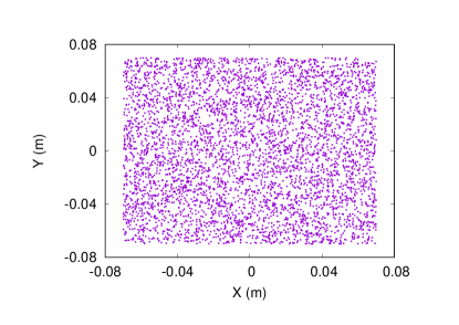
Figure 4: A uniformly distributed LAFE. Each point denotes the position of an emitter.

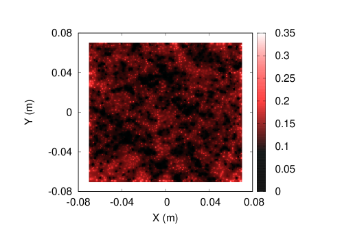
Figure 5: The corresponding current map of the LAFE. The dark regions have low electron emission. The current is measured in amperes.

$$I_{{\bf LAFE}}=\sum\limits_{i}I_{i}=2\pi R_{a}^{2}\sum\limits_{i}J_{a_{i}}{\cal G}_{i}$$ (45)

where $I_{a_{i}}$ is the current from the $i^{\rm th}$ emitter and the corresponding apex current density is

$$J_{a_{i}}=\frac{1}{t_{F_{i}}^{2}}\frac{A_{\small{\rm FN}}}{\phi}E_{a_{i}}^{2}~{}e^{-B_{\small{\rm FN}}\nu_{F_{i}}\phi^{3/2}/E_{a_{i}}}.$$ (46)

while the area-factor is

$${\cal G}_{i}=\frac{E_{a_{i}}}{B_{{\small{\rm FN}}}\phi^{3/2}}\frac{1}{(1-f_{0i}/6)}.$$ (47)

In the above, $E_{a_{i}}~{}=~{}\gamma_{a_{i}}~{}E_{0}$ is the local field at the apex of the $i^{\rm th}$ emitter, $\gamma_{a_{i}}$ is the apex enhancement factor and $E_{0}$ is the asymptotic electric field. Here, $A_{\small{\rm FN}}~{}\simeq~{}1.541434~{}{\rm\mu A~{}eV~{}V}^{-2}$ and $B_{\small{\rm FN}}~{}\simeq~{}6.830890~{}{\rm eV}^{-3/2}~{}{\rm V~{}nm}^{-1}$ are the conventional FN constants, $\phi$ is the work function while $\nu_{F_{i}}\simeq 1-f_{0i}+\frac{1}{6}f_{0i}\ln f_{0i}$ and $t_{F_{i}}\simeq$ $1+f_{0i}/9-\frac{1}{18}f_{0i}\ln f_{0i}$ are correction factors due to the image potential with $f_{0i}\simeq c_{S}^{2}E_{a_{i}}/\phi^{2}$ and $c_{S}^{2}=1.439965~{}{\rm eV^{2}~{}V^{-1}~{}nm}$. Unless otherwise stated, the work function $\phi=4.5$eV in this paper.

Fig. 4 shows the position of 4900 uniformly distributed emitters with mean separation $2000~{}\mu$m. The corresponding current map is shown in Fig. 5. It can be seen that sparse regions have high electron emission while denser regions have lower emission.

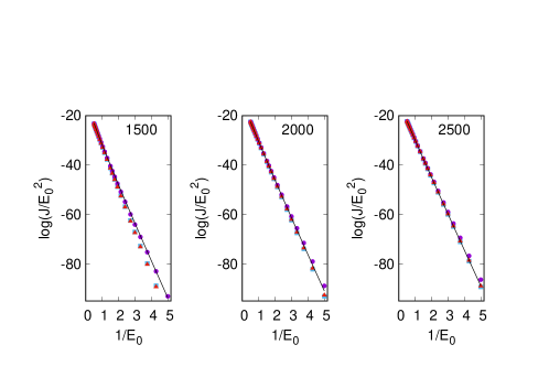
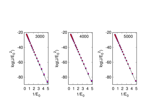
Figure 6: A comparison of the FN plots for the LAFE current density for 6 mean separations found by (a) summing individual emitter currents using exact AFEF (continuous curve) (b) using Gumbel distribution and approximate analytical $\gamma_{a}^{(i)}$ (Eq. 25) to find $\mu$ and $\sigma$ and hence the Gumbel parameters ($\blacksquare$) (c) using Gumbel distribution and approximate analytical $\gamma_{a}^{(i)}$ (Eq. 25) to find $\mu_{h}$ and $\sigma_{h}$ using pair-wise distribution ($\blacktriangle$) (d) using Gaussian distribution and approximate analytical $\gamma_{a}^{(i)}$ (Eq. 25) to find $\mu$ and $\sigma$ ($\CIRCLE$). The mean separations are $1500~{}\mu$m (top-left), $2000~{}\mu$m (top-middle), $2500~{}\mu$m (top-right), $1500~{}\mu$m (bottom-left), $2000~{}\mu$m (bottom-middle), $2500~{}\mu$m (bottom-right). Cases (b) and (c) are virtually indistinguishable. The X-axis has units of $\mu$m/V, while $J/E_{0}^{2}$ has units of $A/V^{2}$. The Gaussian distribution over-estimates the current for mean separations greater than $2000~{}\mu$m.

The net current from the LAFE can alternately be calculated using the apex field enhancement factor distribution. Using an AFEF distribution, the summation in Eq. 45 can be expressed as

$$I_{{\bf LAFE}}=\sum\limits_{i}I_{i}=2\pi R_{a}^{2}\int\limits_{0}^{\infty}J_{a}(x){\cal G}(x)f_{\gamma}(x)dx$$ (48)

where $f_{\gamma}(x)$ is the Gumbel distribution and

$$J_{a}(x) = \frac{1}{t_{F}^{2}(x)}\frac{A_{\small{\rm FN}}}{\phi}E_{a}^{2}(x)~{}e^{-B_{\small{\rm FN}}\nu_{F}(x)\phi^{3/2}/E_{a}(x)}$$ (49)

$${\cal G}(x) = \frac{E_{a}(x)}{B_{{\small{\rm FN}}}\phi^{3/2}}\frac{1}{(1-f_{0}(x)/6)}$$ (50)

$$\nu_{F}(x) = 1-f_{0}(x)+\frac{1}{6}f_{0}(x)\ln f_{0}(x)$$ (51)

$$t_{F}(x) \simeq 1+\frac{1}{9}f_{0}(x)-\frac{1}{18}f_{0}(x)\ln f_{0}(x)$$ (52)

$$f_{0}(x) \simeq c_{S}^{2}E_{a}(x)/\phi^{2}.$$ (53)

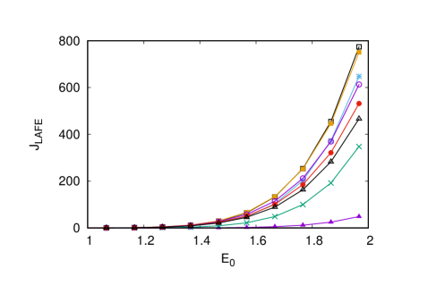
Figure 7: A comparison of the exact LAFE current density ($\text{A/m}^{2}$) for different mean separations is shown as a function of the asymptotic field $E_{0}~{}\text{(V/}\mu\text{m)}$. The mean separations in units of $\mu$m are 1000 ($\blacktriangle$), 1500 (${\bm{\times}}$), 2000 (${\bm{\ast}}$), 2500 (${\bm{\Box}}$), 3000 ($\blacksquare$), 4000 (${\bigcirc}$), 4500 ($\CIRCLE$) and 5000 (${\bm{\triangle}}$).

In Fig. 6, the net current obtained by summing over individual pins (continuous curve) is compared with the current obtained using Gaussian/Gumbel AFEF distributions, as a Fowler-Nordheim (FN) plot for different mean separations. The parameters of the Gumbel distribution are obtained in 2 ways. In the first ($\blacksquare$), the mean and standard deviation of $\{\gamma_{a}^{(i)}\}$ (obtained from Eq. 25 for a given realization of uniform distribution), are used to evaluate $\alpha$ and $\beta$ (Eqns. 28 and 29). In the second ($\blacktriangle$), $\alpha$ and $\beta$ are obtained using the harmonic mean and standard deviation which in turn are evaluated using the pairwise distribution. Also shown is the current obtained using a Gaussian distribution with $\mu$ and $\sigma$ obtained using $\{\gamma_{a}^{(i)}\}$ ($\CIRCLE$). The agreement with the Gumbel distribution is reasonably good at all the separations except when the mean separation equals the emitter height where the Gaussian distribution performs much better especially at lower field strengths. The Gumbel distribution performs well even at low field strengths and notably even when the parameters are obtained using the pairwise distribution. Note that even though a wide range of external asymptotic fields $E_{0}$ has been investigated, for practical purposes, values of $\ln(J/E_{0}^{2})$ exceeding -50 are relevant.

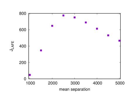
Figure 8: Variation of the exact LAFE current density ($\text{A/m}^{2}$) with mean separation ($\mu$m) at $E_{0}\simeq 1.96$ V/$\mu$m.

Finally, we investigate the optimal mean separation at which the emission current density for the random LAFE considered here is maximum. Fig. 7 shows the current density plotted against the asymptotic electrostatic field $E_{0}$ for various mean separations. The maximum current density peaks sharply after the mean separation crosses the emitter height (1500 $\mu$m) and plateaus at around 2500-3000 $\mu$m for all field strengths (see Fig. 8 for the variation of current density with mean separation at $E_{0}\simeq 1.96$ V/nm). This is similar to the trend seen for an infinite array jap2016 .

V Summary and Conclusions

We have studied shielding effects in a random large area field emitter starting with a 2-emitter system. Methods similar to one used in recently db_fef were used to first arrive at a formula for the apex field enhancement factor (AFEF) in a 2-emitter system and this was subsequently generalized for an arbitrary N-emitter system where the emitter placements may be in a line, a 2-dimensional array or even randomly distributed. It was found that for purposes of field emission where emitters with the largest AFEFs contribute, the shielding effect can be considered to be purely geometric and the AFEFs can be determined, within acceptable limits, purely from the emitter locations without solving the full electrostatic problem.

The question of AFEF distribution was subsequently investigated. It was found that the distribution is closer to a Gaussian when the mean separation is close to or somewhat less than the emitter height, but is better approximated by a Gumbel minimum distribution for spacings larger than emitter height. It is in this regime that the maximum LAFE current density is found to lie.

These results are supported by computation of the emission current, both, by directly summing over individual pins after solving the full electrostatic problem, and at the other extreme by using the expression for approximate (geometric) analytical AFEFs together with the Gumbel and Gaussian distributions. The comparison shows that the latter method with Gumbel distribution can be used profitably for a large range of field strengths for mean separations larger than the emitter height but at mean separations close to the emitter height, the Gaussian distribution performs much better.

Finally, for the uniform distribution of emitters, we have evaluated the Gumbel parameters using the pair-wise distance distribution by calculating the harmonic mean and standard deviation. The evaluation of current using these parameters gives excellent results (for mean separation greater than emitter height) that are virtually indistinguishable from results with parameter obtained from a given realization of the emitter pins.

VI Acknowledgements

The authors thank Raghwendra Kumar, Gaurav Singh and Rajasree for useful discussions.

VII References

References

- (1) K. B. K. Teo, E. Minoux, L. Hudanski, F. Peauger, J. P. Schnell, L. Gangloff, P. Legagneux, D. Dieumegard, G. .A.J. Amaratunga and W. I. Milne, Nature 437, 968 (2005).
- (2) R. J. Parmee, C. M. Collins, W. I. Milne, and M. T. Cole, Nano Convergence 2, 1 (2015).
- (3) C. A. Spindt, J. Appl. Phys., 39, 3504 (1968).
- (4) C. A. Spindt, I. Brodie, L. Humphrey, and E. R. Westerberg, J. Appl. Phys. 47, 5248 (1976).
- (5) C. A. Spindt, C. E. Holland, A. Rosengreen and I. Brodie, IEEE Trans. on Electron Devices, 38, 2355 (1991).
- (6) W. A. de Heer, A. Châtelain and D. Ugarte, Science 270, 1179 (5239).
- (7) M. T. Cole, K. B. K. Teo, O. Groening, L. Gangloff, P. Legagneux, and W. I. Milne, Sci. Rep. 4, 4840 (2014).
- (8) A. I. Zhbanov, E. G. Pogorelov, Y.-C. Chang, and Y.-G. Lee, J. Appl. Phys. 110, 114311 (2011).
- (9) R. G. Forbes, Nanotechnology 23, 095706 (2012).
- (10) F. H. Read and N. J. Bowring, Nucl. Instrum. Meth. Phys. Res. A 519, 305 (2004).
- (11) J. R. Harris, K. L. Jensen, D. A. Shiffler and J. J. Petillo, Appl. Phys. Lettrs. 106, 201603 (2015).
- (12) R. Forbes, J. App. Phys. 120, 054302 (2016).
- (13) K. L. Jensen, Field emission - fundamental theory to usage, Wiley Encycl. Electr. Electron. Eng. (2014).
- (14) D. Biswas, G. Singh and R. Kumar, J. App. Phys. 120, 124307 (2016).
- (15) K. L. Jensen, D. A. Shiffler, J. R. Harris, I. M. Rittersdorf, and J. J. Pettilo, J. Vac. Sci. Technol., B 35, 02C101 (2017).
- (16) D. Biswas and R. Rajasree, Phys. Plasmas, 24, 073107 (2017); 24, 079901 (2017).
- (17) D. Biswas, R. Rajasree and G. Singh, Phys. Plasmas 25, 013113 (2018).
- (18) R. H. Fowler and L. Nordheim, Proc. R. Soc. A 119, 173 (1928).
- (19) E. L. Murphy and R. H. Good, Phys. Rev. 102, 1464 (1956).
- (20) R. G. Forbes, App. Phys. Lett. 89, 113122 (2006).
- (21) R. G. Forbes and J. H. B. Deane, Proc. Roy. Soc. A 463, 2907 (2007).
- (22) R. G. Forbes, C.J. Edgcombe and U. Valdrè, Ultramicroscopy 95, 57 (2003).
- (23) D. Biswas, Phys. Plasmas 25, 043113 (2018).
- (24) L. Nilsson, O. Groening, P. Groening, O. Kuettel, and L. Schlapbach, J. App. Phys. 90, 768 (2001).
- (25) F. Andrianiazy, Jean-Paul Mazellier, L. Sabaut, L. Gangloff, P. Legagneux, and O. Groening, J. Vac. Sci. Tech. B, 33, 012201 (2015).
- (26) T .A. de Assis and F. F. Dall’Agnol,J . Phys.: Condens. Matter 30, 195301 (2018).
- (27) R. G. Forbes, https://arxiv.org/abs/1803.03167 (2018).
- (28) J. Philip, TRITA MAT, 7 (10) (2007).
- (29) D. Biswas, G. Singh, S. G. Sarkar and R. Kumar, Ultramicroscopy 185, 1 (2018).
- (30) D. Biswas, Phys. Plasmas 25, 043105 (2018).