Learning 3D Shape Completion under Weak Supervision

Abstract

We address the problem of 3D shape completion from sparse and noisy point clouds, a fundamental problem in computer vision and robotics. Recent approaches are either data-driven or learning-based: Data-driven approaches rely on a shape model whose parameters are optimized to fit the observations; Learning-based approaches, in contrast, avoid the expensive optimization step by learning to directly predict complete shapes from incomplete observations in a fully-supervised setting. However, full supervision is often not available in practice. In this work, we propose a weakly-supervised learning-based approach to 3D shape completion which neither requires slow optimization nor direct supervision. While we also learn a shape prior on synthetic data, we amortize, i.e., learn, maximum likelihood fitting using deep neural networks resulting in efficient shape completion without sacrificing accuracy. On synthetic benchmarks based on ShapeNet (Chang et al, 2015) and ModelNet (Wu et al, 2015) as well as on real robotics data from KITTI (Geiger et al, 2012) and Kinect (Yang et al, 2018), we demonstrate that the proposed amortized maximum likelihood approach is able to compete with the fully supervised baseline of Dai et al (2017) and outperforms the data-driven approach of Engelmann et al (2016), while requiring less supervision and being significantly faster.

1 Introduction

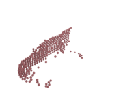
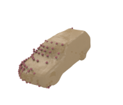
(a) ShapeNet (Synthetic)

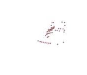
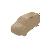
(b) KITTI (Real)

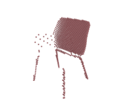
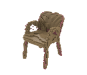
(c) ModelNet (Synthetic)

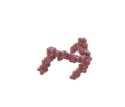
(d) Kinect (Real)

Figure 2: 3D Shape Completion. Results for cars on ShapeNet (Chang et al, 2015) and KITTI (Geiger et al, 2012) and for chairs and tables on ModelNet (Wu et al, 2015) and Kinect (Yang et al, 2018). Learning shape completion on real-world data is challenging due to sparse and noisy observations and missing ground truth. Occupancy grids (bottom) or meshes from signed distance functions (SDFs, top) at various resolutions in beige and point cloud observations in red.

Figure 3: Amortized Maximum Likelihood (AML) for 3D Shape Completion on KITTI. (1) We train a denoising variational auto-encoder (DVAE) (Kingma and Welling, 2014; Im et al, 2017) as shape prior on ShapeNet using occupancy grids and signed distance functions (SDFs) to represent shapes. (2) The fixed generative model, i.e., decoder, then allows to learn shape completion using an unsupervised maximum likelihood (ML) loss by training a new recognition model, i.e., encoder. The retained generative model constraints the space of possible shapes while the ML loss aligns the predicted shape with the observations.

3D shape perception is a long-standing and fundamental problem both in human and computer vision (Pizlo, 2007, 2010; Furukawa and Hernandez, 2013) with many applications to robotics. A large body of work focuses on 3D reconstruction, e.g., reconstructing objects or scenes from one or multiple views, which is an inherently ill-posed inverse problem where many configurations of shape, color, texture and lighting may result in the very same image. While the primary goal of human vision is to understand how the human visual system accomplishes such tasks, research in computer vision and robotics is focused on the task of devising 3D reconstruction systems. Generally, work by Pizlo (2010) suggests that the constraints and priors used for 3D perception are innate and not learned. Similarly, in computer vision, cues and priors are commonly built into 3D reconstruction pipelines through explicit assumptions. Recently, however – leveraging the success of deep learning – researchers started to learn shape models from large collections of data, as for example ShapeNet (Chang et al, 2015). Predominantly generative models have been used to learn how to generate, manipulate and reason about 3D shapes (Girdhar et al, 2016; Brock et al, 2016; Sharma et al, 2016; Wu et al, 2016b, 2015).

In this paper, we focus on the specific problem of inferring and completing 3D shapes based on sparse and noisy 3D point observations as illustrated in Fig. 2. This problem occurs when only a single view of an individual object is provided or large parts of the object are occluded as common in robotic applications. For example, autonomous vehicles are commonly equipped with LiDAR scanners providing a 360 degree point cloud of the surrounding environment in real-time. This point cloud is inherently incomplete: back and bottom of objects are typically occluded and – depending on material properties – the observations are sparse and noisy, see Fig. 2 (top-right) for an illustration. Similarly, indoor robots are generally equipped with low-cost, real-time RGB-D sensors providing noisy point clouds of the observed scene. In order to make informed decisions (e.g., for path planning and navigation), it is of utmost importance to efficiently establish a representation of the environment which is as complete as possible.

Existing approaches to 3D shape completion can be categorized into data-driven and learning-based methods. The former usually rely on learned shape priors and formulate shape completion as an optimization problem over the corresponding (lower-dimensional) latent space (Rock et al, 2015; Haene et al, 2014; Li et al, 2015; Engelmann et al, 2016; Nan et al, 2012; Bao et al, 2013; Dame et al, 2013; Nguyen et al, 2016). These approaches have demonstrated good performance on real data, e.g., on KITTI (Geiger et al, 2012), but are often slow in practice.

Learning-based approaches, in contrast, assume a fully supervised setting in order to directly learn shape completion on synthetic data (Riegler et al, 2017a; Smith and Meger, 2017; Dai et al, 2017; Sharma et al, 2016; Fan et al, 2017; Rezende et al, 2016; Yang et al, 2018; Wang et al, 2017; Varley et al, 2017; Han et al, 2017). They offer advantages in terms of efficiency as prediction can be performed in a single forward pass, however, require full supervision during training. Unfortunately, even multiple, aggregated observations (e.g., from multiple views) will not be fully complete due to occlusion, sparse sampling of views and noise, see Fig. 22 (right column) for an example.

In this paper, we propose an amortized maximum likelihood approach for 3D shape completion (cf. Fig. 3) avoiding the slow optimization problem of data-driven approaches and the required supervision of learning-based approaches. Specifically, we first learn a shape prior on synthetic shapes using a (denoising) variational auto-encoder (Im et al, 2017; Kingma and Welling, 2014). Subsequently, 3D shape completion can be formulated as a maximum likelihood problem. However, instead of maximizing the likelihood independently for distinct observations, we follow the idea of amortized inference (Gershman and Goodman, 2014) and learn to predict the maximum likelihood solutions directly. Towards this goal, we train a new encoder which embeds the observations in the same latent space using an unsupervised maximum likelihood loss. This allows us to learn 3D shape completion in challenging real-world situations, e.g., on KITTI, and obtain sub-voxel accurate results using signed distance functions at resolutions up to $64^{3}$ voxels. For experimental evaluation, we introduce two novel, synthetic shape completion benchmarks based on ShapeNet and ModelNet (Wu et al, 2015). We compare our approach to the data-driven approach by Engelmann et al (2016), a baseline inspired by Gupta et al (2015) and the fully-supervised learning-based approach by Dai et al (2017); we additionally present experiments on real data from KITTI and Kinect (Yang et al, 2018). Experiments show that our approach outperforms data-driven techniques and rivals learning-based techniques while significantly reducing inference time and using only a fraction of supervision.

A preliminary version of this work has been published at CVPR’18 (Stutz and Geiger, 2018). However, we improved the proposed shape completion method, the constructed datasets and present more extensive experiments. In particular, we extended our weakly-supervised amortized maximum likelihood approach to enforce more variety and increase visual quality significantly. On ShapeNet and ModelNet, we use volumetric fusion to obtain more detailed, watertight meshes and manually selected – per object-category – $220$ high-quality models to synthesize challenging observations. We additionally increased the spatial resolution and consider two additional baselines (Dai et al, 2017; Gupta et al, 2015). Our code and datasets will be made publicly available.

The paper is structured as follows: We discuss related work in Section 2. In Section 3 we introduce the weakly-supervised shape completion problem and describe the proposed amortized maximum likelihood approach. Subsequently, we introduce our synthetic shape completion benchmarks and discuss the data preparation for KITTI and Kinect in Section 4.1. Next, we discuss evaluation in Section 4.2, our training procedure in Section 4.3, and the evaluated baselines in Section 4.4. Finally, we present experimental results in Section 4.5 and conclude in Section 5.

2 Related Work

2.1 3D Shape Completion and Single-View 3D Reconstruction

In general, 3D shape completion is a special case of single-view 3D reconstruction where we assume point cloud observations to be available, e.g. from laser-based sensors as on KITTI (Geiger et al, 2012).

3D Shape Completion: Following Sung et al (2015), classical shape completion approaches can roughly be categorized into symmetry-based methods and data-driven methods. The former leverage observed symmetry to complete shapes; representative works include (Thrun and Wegbreit, 2005; Pauly et al, 2008; Zheng et al, 2010; Kroemer et al, 2012; Law and Aliaga, 2011). Data-driven approaches, in contrast, as pioneered by Pauly et al (2005), pose shape completion as retrieval and alignment problem. While Pauly et al (2005) allow shape deformations, Gupta et al (2015), use the iterative closest point (ICP) algorithm (Besl and McKay, 1992) for fitting rigid shapes. Subsequent work usually avoids explicit shape retrieval by learning a latent space of shapes (Rock et al, 2015; Haene et al, 2014; Li et al, 2015; Engelmann et al, 2016; Nan et al, 2012; Bao et al, 2013; Dame et al, 2013; Nguyen et al, 2016). Alignment is then formulated as optimization problem over the learned, low-dimensional latent space. For example, Bao et al (2013) parameterize the shape prior through anchor points with respect to a mean shape, while Engelmann et al (2016) and Dame et al (2013) directly learn the latent space using principal component analysis and Gaussian process latent variable models (Prisacariu and Reid, 2011), respectively. In these cases, shapes are usually represented by signed distance functions (SDFs). Nguyen et al (2016) use 3DShapeNets (Wu et al, 2015), a deep belief network trained on occupancy grids, as shape prior. In general, data-driven approaches are applicable to real data assuming knowledge about the object category. However, inference involves a possibly complex optimization problem, which we avoid by amortizing, i.e., learning, the inference procedure. Additionally, we also consider multiple object categories.

With the recent success of deep learning, several learning-based approaches have been proposed (Firman et al, 2016; Smith and Meger, 2017; Dai et al, 2017; Sharma et al, 2016; Rezende et al, 2016; Fan et al, 2017; Riegler et al, 2017a; Han et al, 2017; Yang et al, 2017, 2018). Strictly speaking, these are data-driven, as well; however, shape retrieval and fitting are both avoided by directly learning shape completion end-to-end, under full supervision – usually on synthetic data from ShapeNet (Chang et al, 2015) or ModelNet (Wu et al, 2015). Riegler et al (2017a) additionally leverage octrees to predict higher-resolution shapes; most other approaches use low resolution occupancy grids (e.g., $32^{3}$ voxels). Instead, Han et al (2017) use a patch-based approach to obtain high-resolution results. In practice, however, full supervision is often not available; thus, existing models are primarily evaluated on synthetic datasets. In order to learn shape completion without full supervision, we utilize a learned shape prior to constrain the space of possible shapes. In addition, we use SDFs to obtain sub-voxel accuracy at higher resolutions (up to $48\operatorname*{\!\times\!}108\operatorname*{\!\times\!}48$ or $64^{3}$ voxels) without using patch-based refinement or octrees. We also consider significantly sparser observations.

Single-View 3D Reconstruction: Single-view 3D reconstruction has received considerable attention over the last years; we refer to (Oswald et al, 2013) for an overview and focus on recent deep learning approaches, instead. Following Tulsiani et al (2018), these can be categorized by the level of supervision. For example, (Girdhar et al, 2016; Choy et al, 2016; Wu et al, 2016b; Häne et al, 2017) require full supervision, i.e., pairs of images and ground truth 3D shapes. These are generally derived synthetically. More recent work (Yan et al, 2016; Tulsiani et al, 2017, 2018; Kato et al, 2017; Lin et al, 2017; Fan et al, 2017; Tatarchenko et al, 2017; Wu et al, 2016a), in contrast, self-supervise the problem by enforcing consistency across multiple input views. Tulsiani et al (2018), for example, use a differentiable ray consistency loss; and in (Yan et al, 2016; Kato et al, 2017; Lin et al, 2017), differentiable rendering allows to define reconstruction losses on the images directly. While most of these approaches utilize occupancy grids, Fan et al (2017) and Lin et al (2017) predict point clouds instead. Tatarchenko et al (2017) use octrees to predict higher-resolution shapes. Instead of employing multiple views as weak supervision, however, we do not assume any additional views in our approach. Instead, knowledge about the object category is sufficient. In this context, concurrent work by Gwak et al (2017) is more related to ours: a set of reference shapes implicitly defines a prior of shapes which is enforced using an adversarial loss. In contrast, we use a denoising variational auto-encoder (DVAE) (Kingma and Welling, 2014; Im et al, 2017) to explicitly learn a prior for 3D shapes.

2.2 Shape Models

Shape models and priors found application in a wide variety of different tasks. In 3D reconstruction, in general, shape priors are commonly used to resolve ambiguities or specularities (Dame et al, 2013; Güney and Geiger, 2015; Kar et al, 2015). Furthermore, pose estimation (Sandhu et al, 2011, 2009; Prisacariu et al, 2013; Aubry et al, 2014), tracking (Ma and Sibley, 2014; Leotta and Mundy, 2009), segmentation (Sandhu et al, 2011, 2009; Prisacariu et al, 2013), object detection (Zia et al, 2013, 2014; Pepik et al, 2015; Song and Xiao, 2014; Zheng et al, 2015) or recognition (Lin et al, 2014) – to name just a few – have been shown to benefit from shape models. While most of these works use hand-crafted shape models, for example based on anchor points or part annotations (Zia et al, 2013, 2014; Pepik et al, 2015; Lin et al, 2014), recent work (Liu et al, 2017; Sharma et al, 2016; Girdhar et al, 2016; Wu et al, 2016b, 2015; Smith and Meger, 2017; Nash and Williams, 2017; Liu et al, 2017) has shown that generative models such as VAEs (Kingma and Welling, 2014) or generative adversarial networks (GANs) (Goodfellow et al, 2014) allow to efficiently generate, manipulate and reason about 3D shapes. We use these more expressive models to obtain high-quality shape priors for various object categories.

2.3 Amortized Inference

To the best of our knowledge, the notion of amortized inference was introduced by Gershman and Goodman (2014) and picked up repeatedly in different contexts (Rezende and Mohamed, 2015; Wang et al, 2016; Ritchie et al, 2016). Generally, it describes the idea of learning to infer (or learning to sample). We refer to (Wang et al, 2016) for a broader discussion of related work. In our context, a VAE can be seen as specific example of learned variational inference (Kingma and Welling, 2014; Rezende and Mohamed, 2015). Besides using a VAE as shape prior, we also amortize the maximum likelihood problem corresponding to our 3D shape completion task.

3 Method

In the following, we introduce the mathematical formulation of the weakly-supervised 3D shape completion problem. Subsequently, we briefly discuss denoising variational auto-encoders (DVAEs) (Kingma and Welling, 2014; Im et al, 2017) which we use to learn a strong shape prior that embeds a set of reference shapes in a low-dimensional latent space. Then, we formally derive our proposed amortized maximum likelihood (AML) approach. Here, we use maximum likelihood to learn an embedding of the observations within the same latent space – thereby allowing to perform shape completion. The overall approach is also illustrated in Fig. 3.

3.1 Problem Formulation

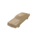
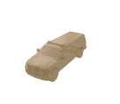
(a) Reference Shapes $\mathcal{Y}$

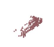
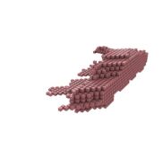
(b) Observation $x_{n}$

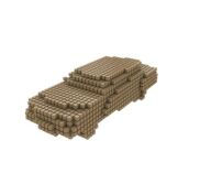
(c) Ground Truth $y_{n}^{*}$

Figure 5: Weakly-Supervised Shape Completion. Given reference shapes $\mathcal{Y}$ and incomplete observations $\mathcal{X}$, we want to learn a mapping $x_{n}\mapsto\tilde{y}(x_{n})$ such that $\tilde{y}(x_{n})$ matches the unknown ground truth shape $y_{n}^{*}$ as close as possible. The observations $x_{n}$ are split into free space (i.e., $x_{n,i}=0$, right) and point observations (i.e., $x_{n,i}=1$, left). Shapes are shown in beige and observations in red.

In a supervised setting, the task of 3D shape completion can be described as follows: Given a set of incomplete observations $\mathcal{X}=\{x_{n}\}_{n=1}^{N}\subseteq\mathbb{R}^{R}$ and corresponding ground truth shapes $\mathcal{Y}^{*}=\{y_{n}^{*}\}_{n=1}^{N}\subseteq\mathbb{R}^{R}$, learn a mapping $x_{n}\mapsto y_{n}^{*}$ that is able to generalize to previously unseen observations and possibly across object categories. We assume $\mathbb{R}^{R}$ to be a suitable representation of observations and shapes; in practice, we resort to occupancy grids and signed distance functions (SDFs) defined on regular grids, i.e., $x_{n},y_{n}^{*}\in\mathbb{R}^{H\operatorname*{\!\times\!}W\operatorname*{\!\times\!}D}\simeq\mathbb{R}^{R}$. Specifically, occupancy grids indicate occupied space, i.e., voxel $y_{n,i}^{*}=1$ if and only if the voxel lies on or inside the shape’s surface. To represent shapes with sub-voxel accuracy, SDFs hold the distance of each voxel’s center to the surface; for voxels inside the shape’s surface, we use negative sign. Finally, for the (incomplete) observations, we write $x_{n}\in\{0,1,\bot\}^{R}$ to make missing information explicit; in particular, $x_{n,i}=\bot$ corresponds to unobserved voxels, while $x_{n,i}=1$ and $x_{n,i}=0$ correspond to occupied and unoccupied voxels, respectively.

On real data, e.g., KITTI (Geiger et al, 2012), supervised learning is often not possible as obtaining ground truth annotations is labor intensive, cf. (Menze and Geiger, 2015; Xie et al, 2016). Therefore, we target a weakly-supervised variant of the problem instead: Given observations $\mathcal{X}$ and reference shapes $\mathcal{Y}=\{y_{m}\}_{m=1}^{M}\subseteq\mathbb{R}^{R}$ both of the same, known object category, learn a mapping $x_{n}\mapsto\tilde{y}(x_{n})$ such that the predicted shape $\tilde{y}(x_{n})$ matches the unknown ground truth shape $y_{n}^{*}$ as close as possible – or, in practice, the sparse observation $x_{n}$ while being plausible considering the set of reference shapes, cf. Fig. 5. Here, supervision is provided in the form of the known object category. Alternatively, the reference shapes $\mathcal{Y}$ can also include multiple object categories resulting in an even weaker notion of supervision as the correspondence between observations and object categories is unknown. Except for the object categories, however, the set of reference shapes $\mathcal{Y}$, and its size $M$, is completely independent of the set of observations $\mathcal{X}$, and its size $N$, as also highlighted in Fig. 3. On real data, e.g., KITTI, we additionally assume the object locations to be given in the form of 3D bounding boxes in order to extract the corresponding observations $\mathcal{X}$. In practice, the reference shapes $\mathcal{Y}$ are derived from watertight, triangular meshes, e.g., from ShapeNet (Chang et al, 2015) or ModelNet (Wu et al, 2015).

3.2 Shape Prior

We approach the weakly-supervised shape completion problem by first learning a shape prior using a denoising variational auto-encoder (DVAE). Later, this prior constrains shape inference (see Section 3.3) to predict reasonable shapes. In the following, we briefly discuss the standard variational auto-encoder (VAE), as introduced by Kingma and Welling (2014), as well as its denoising extension, as proposed by Im et al (2017).

Variational Auto-Encoder (VAE): We propose to use the provided reference shapes $\mathcal{Y}$ to learn a generative model of possible 3D shapes over a low-dimensional latent space $\mathcal{Z}=\mathbb{R}^{Q}$, i.e., $Q\ll R$. In the framework of VAEs, the joint distribution $p(y,z)$ of shapes $y$ and latent codes $z$ decomposes into $p(y|z)p(z)$ with $p(z)$ being a unit Gaussian, i.e., $\mathcal{N}(z;0,I_{Q})$ and $I_{Q}\in\mathbb{R}^{R\times R}$ being the identity matrix. This decomposition allows to sample $z\sim p(z)$ and $y\sim p(y|z)$ to generate random shapes. For training, however, we additionally need to approximate the posterior $p(z|y)$. To this end, the so-called recognition model $q(z|y)\approx p(z|y)$ takes the form

$$q(z|y) =\mathcal{N}(z;\mu(y),\text{diag}(\sigma^{2}(y)))$$ (1)

where $\mu(y),\sigma^{2}(y)\in\mathbb{R}^{Q}$ are predicted using the encoder neural network. The generative model $p(y|z)$ decomposes over voxels $y_{i}$; the corresponding probabilities $p(y_{i}|z)$ are represented using Bernoulli distributions for occupancy grids or Gaussian distributions for SDFs:

$$\begin{split}p(y_{i}|z)&=\text{Ber}(y_{i};\theta_{i}(z))\quad\text{or}\\ p(y_{i}|z)&=\mathcal{N}(y_{i};\mu_{i}(z),\sigma^{2}).\end{split}$$ (2)

In both cases, the parameters, i.e., $\theta_{i}(z)$ or $\mu_{i}(z)$, are predicted using the decoder neural network. For SDFs, we explicitly set $\sigma^{2}$ to be constant (see Section 4.3). Then, $\sigma^{2}$ merely scales the corresponding loss, thereby implicitly defining the importance of accurate SDFs relative to occupancy grids as described below.

In the framework of variational inference, the parameters of the encoder and the decoder neural networks are found by maximizing the likelihood $p(y)$. In practice, the likelihood is usually intractable and the evidence lower bound is maximized instead, see (Kingma and Welling, 2014; Blei et al, 2016). This results in the following loss to be minimized:

$$\mathcal{L}_{\text{VAE}}(w)=-\mathbb{E}_{q(z|y)}[\ln p(y|z)]+\text{KL}(q(z|y)|p(z)).$$ (3)

Here, $w$ are the weights of the encoder and decoder hidden in the recognition model $q(z|y)$ and the generative model $p(y|z)$, respectively. The Kullback-Leibler divergence KL can be computed analytically as described in the appendix of (Kingma and Welling, 2014). The negative log-likelihood $-\ln p(y|z)$ corresponds to a binary cross-entropy error for occupancy grids and a scaled sum-of-squared error for SDFs. The loss $\mathcal{L}_{\text{VAE}}$ is minimized using stochastic gradient descent (SGD) by approximating the expectation using samples:

$$-\mathbb{E}_{q(z|y)}[\ln p(y|z)]\approx-\sum_{l=1}^{L}\ln p(y|z^{(l)})$$ (4)

The required samples $z^{(l)}\sim q(z|y)$ are computed using the so-called reparameterization trick,

$$z^{(l)}=\mu(y)+\epsilon^{(l)}\sigma(y)\quad\text{with}\quad\epsilon^{(l)}\sim\mathcal{N}(\epsilon;0,I_{Q}),$$ (5)

in order to make $\mathcal{L}_{\text{VAE}}$, specifically the sampling process, differentiable. In practice, we found $L=1$ samples to be sufficient – which conforms with results by Kingma and Welling (2014). At test time, the sampling process $z\sim q(z|y)$ is replaced by the predicted mean $\mu(y)$. Overall, the standard VAE allows us to embed the reference shapes in a low-dimensional latent space. In practice, however, the learned prior might still include unreasonable shapes.

Denoising VAE (DVAE): In order to avoid inappropriate shapes to be included in our shape prior, we consider a denoising variant of the VAE allowing to obtain a tighter bound on the likelihood $p(y)$. More specifically, a corruption process $y^{\prime}\sim p(y^{\prime}|y)$ is considered and the corresponding evidence lower bound results in the following loss:

$$\begin{split}\mathcal{L}_{\text{DVAE}}(w)=&-\mathbb{E}_{q(z|y^{\prime})}[\ln p(y|z)]\\ &+\text{KL}(q(z|y^{\prime})|p(z)).\end{split}$$ (6)

Note that the reconstruction error $-\ln p(y|z)$ is still computed with respect to the uncorrupted shape $y$ while $z$, in contrast to Eq. (3), is sampled conditioned on the corrupted shape $y^{\prime}$. In practice, the corruption process $p(y^{\prime}|y)$ is modeled using Bernoulli noise for occupancy grids and Gaussian noise for SDFs. In experiments, we found DVAEs to learn more robust latent spaces – meaning the prior is less likely to contain unreasonable shapes. In the following, we always use DVAEs as shape priors.

3.3 Shape Inference

After learning the shape prior, defining the joint distribution $p(y,z)$ of shapes $y$ and latent codes $z$ as product of generative model $p(y|z)$ and prior $p(z)$, shape completion can be formulated as a maximum likelihood (ML) problem for $p(y,z)$ over the lower-dimensional latent space $\mathcal{Z}=\mathbb{R}^{Q}$. The corresponding negative log-likelihood $-\ln p(y,z)$ to be minimized can be written as

$$\mathcal{L}_{\text{ML}}(z) =-\sum_{x_{i}\neq\bot}\ln p(y_{i}=x_{i}|z)-\ln p(z).$$ (7)

As the prior $p(z)$ is Gaussian, the negative log-probability $-\ln p(z)$ is proportional to $\|z\|_{2}^{2}$ and constrains the problem to likely, i.e., reasonable, shapes with respect to the shape prior. As before, the generative model $p(y|z)$ decomposes over voxels; here, we can only consider actually observed voxels $x_{i}\neq\bot$. We assume that the learned shape prior can complete the remaining, unobserved voxels $x_{i}=\bot$. Instead of solving Eq. (7) for each observation $x\in\mathcal{X}$ independently, however, we follow the idea of amortized inference (Gershman and Goodman, 2014) and train a new encoder $z(x;w)$ to learn ML. To this end, we keep the generative model $p(y|z)$ fixed and train only the weights $w$ of the new encoder $z(x;w)$ using the ML objective as loss:

$$\begin{split}\mathcal{L}_{\text{dAML}}(w)=&-\sum_{x_{i}\neq\bot}\ln p(y_{i}=x_{i}|z(x;w))\\ &-\lambda\ln p(z(x;w)).\end{split}$$ (8)

Here, $\lambda$ controls the importance of the shape prior. The exact form of the probabilities $p(y_{i}=x_{i}|z)$ depends on the used shape representation. For occupancy grids, this term results in a cross-entropy error as both the predicted voxels $y_{i}$ and the observations $x_{i}$ are, for $x_{i}\neq\bot$, binary. For SDFs, however, the term is not well-defined as $p(y_{i}|z)$ is modeled with a continuous Gaussian distribution, while the observations $x_{i}$ are binary. As solution, we could compute (signed) distance values along the rays corresponding to observed points (e.g., following (Steinbrucker et al, 2013)) in order to obtain continuous observations $x_{i}\in\mathbb{R}$ for $x_{i}\neq\bot$. However, as illustrated in Fig. 6, noisy observations cause the distance values along the whole ray to be invalid. This can partly be avoided when relying only on occupancy to represent the observations; in this case, free space (cf. Fig. 5) observations are partly correct even though observed points may lie within the corresponding shapes.

For making SDFs tractable (i.e., to predict sub-voxel accurate, visually smooth and appealing shapes, see Section 4.5) while using binary observations, we propose to define $p(y_{i}=x_{i}|z)$ through a simple transformation. In particular, as $p(y_{i}|z)$ is modeled using a Gaussian distribution $\mathcal{N}(y_{i};\mu_{i}(z),\sigma^{2})$ where $\mu_{i}(z)$ is predicted using the fixed decoder ($\sigma^{2}$ is constant), and $x_{i}$ is binary (for $x_{i}\neq\bot$), we introduce a mapping $\theta_{i}(\mu_{i}(z))$ transforming the predicted mean SDF value to an occupancy probability $\theta_{i}(\mu_{i}(z))$:

$$p(y_{i}=x_{i}|z)=\text{Ber}(y_{i}=x_{i};\theta_{i}(\mu_{i}(z)))$$ (9)

As, by construction (see Section 3.1), occupied voxels have negative sign or value zero in the SDF, we can derive the occupancy probability $\theta_{i}(\mu_{i}(z))$ as the probability of a non-positive distance:

$$\theta_{i}(\mu_{i}(z)) =\mathcal{N}(y_{i}\leq 0;\mu_{i}(z),\sigma^{2})$$ (10)

$$=\frac{1}{2}\left(1+\text{erf}\left(\frac{-\mu_{i}(z)}{\sigma\sqrt{\pi}}\right)\right).$$ (11)

Here, erf is the error function which, in practice, can be approximated following (Abramowitz, 1974). Eq. (11) is illustrated in Fig. 6 where the occupancy probability $\theta_{i}(\mu_{i}(z))$ is computed as the area under the Gaussian bell curve for $y_{i}\leq 0$. This per-voxel transformation can easily be implemented as non-linear layer and its derivative wrt. $\mu_{i}(z)$ is, by construction, a Gaussian. Note that the transformation is correct, not approximate, based on our model assumptions and the definitions in Section 3.1. Overall, this transformation allows us to easily minimize Eq. (8) for both occupancy grids and SDFs using binary observations. The obtained encoder embeds the observations in the latent shape space to perform shape completion.

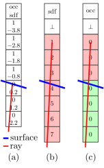
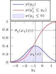
Figure 6: Left: Problem with SDF Observations. Illustration of a ray (red line) correctly hitting a surface (blue line) causing the (signed) distance values and occupancy values computed for voxels along the ray to be correct (cf. (a)). A noisy ray, however, causes all voxels along the ray to be assigned incorrect distance values (marked red) wrt. to the true surface (blue line) because the ray ends far behind the actual surface (cf. (b)). When using occupancy only, in contrast, only the voxels behind the surface are assigned invalid occupancy states (marked red); the remaining voxels are labeled correctly (marked green; cf. (c)). Right: Proposed Gaussian-to-Bernoulli Transformation. For $p(y_{i}):=p(y_{i}|z)=\mathcal{N}(y_{i};\mu_{i}(z),\sigma^{2})$ (blue), we illustrate the transformation discussed in Section 3.3 allowing to use the binary observations $x_{i}$ (for $x_{i}\neq\bot$) to supervise the SDF predictions. This is achieved by transforming the predicted Gaussian distribution to a Bernoulli distribution with occupancy probability $\theta_{i}(\mu_{i}(z))=p(y_{i}\leq 0)$ (blue area).

3.4 Practical Considerations

(a) Original

(b) TSDF Fusion, $256^{3}$

(c) Simplification, $5\text{k}$ Faces

(d) Reconstruction, $24\operatorname*{\!\times\!}54\operatorname*{\!\times\!}24$/$32^{3}$

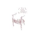
(e) Observations

(f) Voxelization, $24\operatorname*{\!\times\!}54\operatorname*{\!\times\!}24$/$32^{3}$

Figure 8: ShapeNet and ModelNet Data Generation Pipeline. On ShapeNet and ModelNet we illustrate: (8(a)) samples from the original datasets; (8(b)) fused watertight meshes from TSDF fusion at $256^{3}$ voxels resolution using (Riegler et al, 2017a); (8(c)) simplified meshes ($5k$ faces); (8(d)) marching cubes (Lorensen and Cline, 1987) reconstructions from the SDFs computed from (8(c)) (resolutions $24\operatorname*{\!\times\!}54\operatorname*{\!\times\!}24$ and $32^{3}$ voxels; note that steps (8(b)) and (8(c)) are necessary to derive exact SDFs); (8(e)) observations obtained by projection into a single view; and (8(f)) voxelized observations and shapes. Shapes (meshes and occupancy grids) in beige and observations in red.

Encouraging Variety: So far, our AML formulation assumes a deterministic encoder $z(x,w)$ which predicts, given the observation $x$, a single code $z$ corresponding to a completed shape. A closer look at Eq. (8), however, reveals an unwanted problem: the data term scales with the number of observations, i.e., $|\{x_{i}\neq\bot\}|$, while the regularization term stays constant – with less observations, the regularizer gains in importance leading to limited variety in the predicted shapes because $z(x;w)$ tends towards zero.

In order to encourage variety, we draw inspiration from the VAE shape prior. Specifically, we use a probabilistic recognition model

$$q(z|x)=\mathcal{N}(z;\mu(x),\text{diag}(\sigma^{2}(x)))$$ (12)

(cf. see Eq. (1)) and replace the negative log-likelihood $-\ln p(z)$ with the corresponding Kullback-Leibler divergence $\text{KL}(q(z|x)|p(z))$ with $p(z)=\mathcal{N}(z;0,I_{Q})$. Intuitively, this makes sure that the encoder’s predictions “cover” the prior distribution – thereby enforcing variety. Mathematically, the resulting loss, i.e.,

$$\begin{split}\mathcal{L}_{\text{AML}}(w)=&-\mathbb{E}_{q(z|x)}\left[\sum_{x_{i}\neq\bot}\ln p(y_{i}=x_{i}|z)\right]\\ &+\lambda\text{KL}(q(z|x)p(z)),\end{split}$$ (13)

can be interpreted as the result of maximizing the evidence lower bound of a model with observation process $p(x|y)$ (analogously to the corruption process $p(y^{\prime}|y)$ for DVAEs in (Im et al, 2017) and Section 3.2). The expectation is approximated using samples (following the reparameterization trick in Eq. (5)) and, during testing, the sampling process $z\sim q(z|x)$ is replaced by the mean prediction $\mu(x)$. In practice, we find that Eq. (13) improves visual quality of the completed shapes. We compare this AML model to its deterministic variant dAML in Section 4.5.

Handling Noise: Another problem of our AML formulation concerns noise. On KITTI, for example, specular or transparent surfaces cause invalid observations – laser rays traversing through these surfaces cause observations to lie within shapes or not get reflected. However, our AML framework assumes deterministic, i.e., trustworthy, observations – as can be seen in the reconstruction error in Eq. (13). Therefore, we introduce per-voxel weights $\kappa_{i}$ computed using the reference shapes $\mathcal{Y}=\{y_{m}\}_{m=1}^{M}$:

$$\kappa_{i}=1-\left(\frac{1}{M}\sum_{m=1}^{M}y_{m,i}\right)\in[0,1]$$ (14)

where $y_{m,i}=1$ if and only if the corresponding voxel is occupied. Applied to observations $x_{i}=0$, these are trusted less if they are unlikely under the shape prior. Note that for point observations, i.e., $x_{i}=1$, this is not necessary as we explicitly consider “filled” shapes (see Section 4.1). This can also be interpreted as imposing an additional mean shape prior on the predicted shapes with respect to the observed free space. In addition, we use a corruption process $p(x^{\prime}|x)$ consisting of Bernoulli and Gaussian noise during training (analogously to the DVAE shape prior).

4 Experiments

4.1 Data

We briefly introduce our synthetic shape completion benchmarks, derived from ShapeNet (Chang et al, 2015) and ModelNet (Wu et al, 2015) (cf. Fig. 8), and our data preparation for KITTI (Geiger et al, 2012) and Kinect (Yang et al, 2018) (cf. Fig. 10); Table 1 summarizes key statistics including the level of supervision computed as the fraction of observed voxels, i.e. $\nicefrac{{|\{x_{n,i}\neq\bot\}|}}{{HWD}}$, averaged over observations $x_{n}$.

ShapeNet: We utilize the truncated SDF (TSDF) fusion approach of Riegler et al (2017a) to obtain watertight versions of the provided car shapes allowing to reliably and efficiently compute occupancy grids and SDFs. Specifically, we use $100$ depth maps of $640\operatorname*{\!\times\!}640$ pixels resolution, distributed uniformly on the sphere around the shape, and perform TSDF fusion at a resolution of $256^{3}$ voxels. Detailed watertight meshes, without inner structures, can then be extracted using marching cubes (Lorensen and Cline, 1987) and simplified to $5\text{k}$ faces using MeshLab’s quadratic simplification algorithm (Cignoni et al, 2008), see Fig. 8(a) to 8(c). Finally, we manually selected $220$ shapes from this collection, removing exotic cars, unwanted configurations, or shapes with large holes (e.g., missing floors or open windows).

The shapes are splitted into $|\mathcal{Y}|=100$ reference shapes, $|\mathcal{Y}^{*}|=100$ shapes for training the inference model, and $20$ test shapes. We randomly perturb rotation and scaling to obtain $5$ variants of each shape, voxelize them using triangle-voxel intersections and subsequently “fill” the obtained volumes using a connected components algorithm (Jones et al, 2001). For computing SDFs we use SDFGen. We use three different resolutions: $H\operatorname*{\!\times\!}W\operatorname*{\!\times\!}D=24\operatorname*{\!\times\!}54\operatorname*{\!\times\!}24$, $32\operatorname*{\!\times\!}72\operatorname*{\!\times\!}32$ and $48\operatorname*{\!\times\!}108\operatorname*{\!\times\!}48$ voxels. Examples are shown in Fig. 8(d) to 8(f).

Finally, we use the OpenGL renderer of Güney and Geiger (2015) to obtain $10$ depth maps per shape. The incomplete observations $\mathcal{X}$ are obtained by re-projecting them into 3D and marking voxels with at least one point as occupied and voxels between occupied voxels and the camera center as free space. We obtain more dense point clouds at $48\operatorname*{\!\times\!}64$ pixels resolution and sparser point clouds using depth maps of $24\operatorname*{\!\times\!}32$ pixels resolution. For the latter, more challenging case we also add exponentially distributed noise (with rate parameter $70$) to the depth values, or randomly (with probability $0.075$) set them to the maximum depth to simulate the deficiencies of point clouds captured with real sensors, e.g., on KITTI. These two variants are denoted SN-clean and SN-noisy. The obtained observations are illustrated in Fig. 8(e).

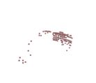
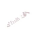
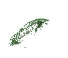
(a) KITTI, Point Clouds

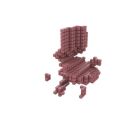
(b) Kinect, Occupancy Grids

Figure 10: Extracted KITTI and Kinect Data. For KITTI, we show observed points in red and the accumulated, partial ground truth in green. Note that for the first example ground truth is not available due to missing past/future observations. For Kinect, we show observations in red and ElasticFusion (Whelan et al, 2015) ground truth in beige. Note that the objects are rotated and not aligned as in ModelNet (cf. Fig. 8).

KITTI: We extract observations from KITTI’s Velodyne point clouds using the provided ground truth 3D bounding boxes to avoid the inaccuracies of 3D object detectors (train/test split by Chen et al (2016)). As the 3D bounding boxes in KITTI fit very tightly, we first padded them by factor $0.25$ on all sides; afterwards, the observed points are voxelized into voxel grids of size $H\operatorname*{\!\times\!}W\operatorname*{\!\times\!}D=24\operatorname*{\!\times\!}54\operatorname*{\!\times\!}24$, $32\operatorname*{\!\times\!}72\operatorname*{\!\times\!}32$ and $48\operatorname*{\!\times\!}108\operatorname*{\!\times\!}48$ voxels. To avoid taking points from the street, nearby walls, vegetation or other objects into account, we only consider those points lying within the original (i.e., not padded) bounding box. Finally, free space is computed using ray tracing as described above. We filter all observations to ensure that each observation contains a minimum of $50$ observations. For the bounding boxes in the test set, we additionally generated partial ground truth by accumulating the 3D point clouds of $10$ future and $10$ past frames around each observation. Examples are shown in Fig. 10.

ModelNet: We use ModelNet10, comprising $10$ popular object categories (bathtub, bed, chair, desk, dresser, monitor, night stand, table, toilet) and select, for each category, the first $200$ and $20$ shapes from the provided training and test sets. Then, we follow the pipeline outlined in Fig. 8, as on ShapeNet, using $10$ random variants per shape. Due to thin structures, however, SDF computation does not work well (especially for low resolution, e.g., $32^{3}$ voxels). Therefore, we approximate the SDFs using a 3D distance transform on the occupancy grids. Our experiments are conducted at a resolution of $H\operatorname*{\!\times\!}W\operatorname*{\!\times\!}D=32^{3}$, $48^{3}$ and $64^{3}$ voxels. Given the increased difficulty, we use a resolution of $64^{2}$, $96^{2}$ and $128^{2}$ pixels for the observation generating depth maps. In our experiments, we consider bathtubs, chairs, desks and tables individually, as well as all $10$ categories together (resulting in $100\text{k}$ views overall). For Kinect, we additionally used a dataset of rotated chairs and tables aligned with Kinect’s ground plane.

	Synthetic		Real
	SN-clean/-noisy	ModelNet	KITTI	Kinect
Training/Test Sets
#Shapes for Shape Prior, #Views for Shape Inference
#Shapes	500/100	1000/200	–	–
#Views	5000/1000	10000/2000	8442/9194	30/10
Observed Voxels in % ($<5\%$) & Resolutions
Low = $24\operatorname*{\!\times\!}54\operatorname*{\!\times\!}24$/$32^{3}$; Medium = $32\operatorname*{\!\times\!}72\operatorname*{\!\times\!}32$/$48^{3}$; High = $48\operatorname*{\!\times\!}108\operatorname*{\!\times\!}48$/$64^{3}$
Low	7.66/3.86	9.71	6.79	0.87
Medium	6.1/2.13	8.74	5.24	–
High	2.78/0.93	8.28	3.44	–

Table 1: Dataset Statistics. We report the number of (rotated and scaled) meshes, used as reference shapes, and the resulting number of observations (i.e., views, $10$ per shape). We also report the average fraction of observed voxels, i.e., $\nicefrac{{|\{x_{i}\neq\bot\}|}}{{HWD}}$. For ModelNet, we exemplarily report statistics for chairs; and for Kinect, we report statistics for tables.

Kinect: Yang et al. provide Kinect scans of various chairs and tables. They provide both single-view observations as well as ground truth from ElasticFusion (Whelan et al, 2015) as occupancy grids. However, the ground truth is not fully accurate, and only $40$ views are provided per object category. Still, the objects have been segmented to remove clutter and are appropriate for experiments in conjunction with ModelNet10. Unfortunately, Yang et al. do not provide SDFs; again, we use 3D distance transforms as approximation. Additionally, the observations do not indicate free space and we were required to guess an appropriate ground plane. For our experiments, we use $30$ views for training and $10$ views for testing, see Fig. 10 for examples.

4.2 Evaluation

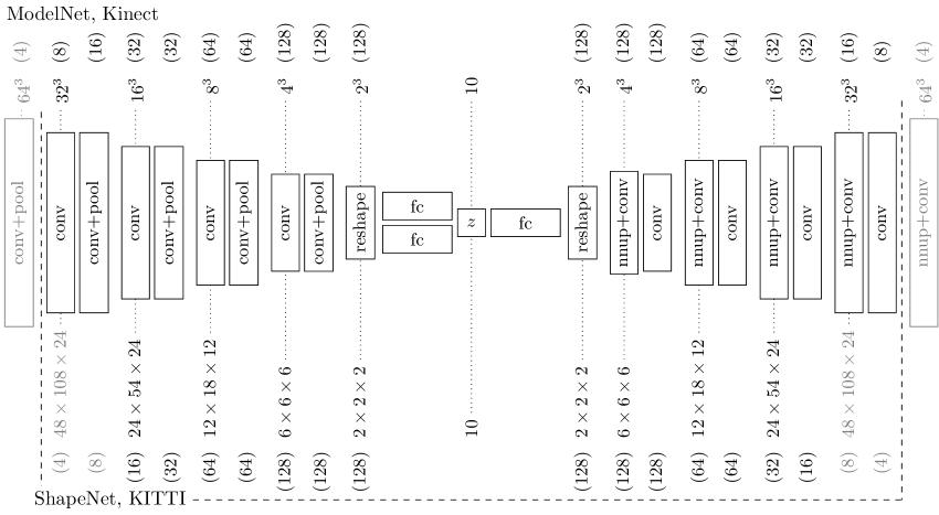
Figure 11: Network Architectures. We use different resolutions for ShapeNet and KITTI as well as ModelNet and Kinect (bottom and top, respectively). In both cases, architectures for higher resolutions employ one additional stage in the en- and decoder (in gray). Each convolutional layer is followed by ReLU activations and batch normalization (Ioffe and Szegedy, 2015); the window sizes for max pooling and nearest-neighbor upsampling can be derived from the context; the number of channels are given in parentheses.

For occupancy grids, we use Hamming distance (Ham) and intersection-over-union (IoU) between the (thresholded) predictions and the ground truth; note that lower Ham is better, while lower IoU is worse. For SDFs, we consider a mesh-to-mesh distance on ShapeNet and a mesh-to-point distance on KITTI. We follow (Jensen et al, 2014) and consider accuracy (Acc) and completeness (Comp). To measure Acc, we uniformly sample roughly $10\text{k}$ points on the reconstructed mesh and average their distance to the target mesh. Analogously, Comp is the distance from the target mesh (or the ground truth points on KITTI) to the reconstructed mesh. Note that for both Acc and Comp, lower is better. On ShapeNet and ModelNet, we report both Acc and Comp in voxels, i.e., in multiples of the voxel edge length (i.e., in [vx], as we do not know the absolute scale of the models); on KITTI, we report Comp in meters (i.e., in [m]).

4.3 Architectures and Training

GT,
High

GT
 

DVAE, Low

DVAE, High

DVAE, Low

DVAE, High

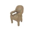
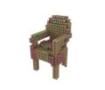
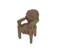
(a) Reconstructions, Low and High Resolution (cf. Table 1)

Low

Low

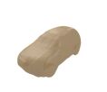
Low

High

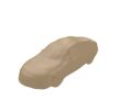
High

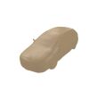
High

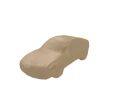
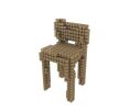
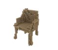
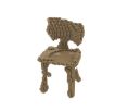
(b) Random Samples, Low and High Resolution (cf. Table 1)

Figure 13: DVAE Shape Prior. Reconstructions and random samples on ShapeNet and ModelNet at multiple resolutions (cf. Table 1); false negative and false positive voxels in green and red. Our DVAE shape prior provides high-quality reconstructions and meaningful random samples across resolutions.

As depicted in Fig. 11, our network architectures are kept simple and shallow. Considering a resolution of $24\operatorname*{\!\times\!}54\operatorname*{\!\times\!}24$ voxels on ShapeNet and KITTI, the encoder comprises three stages, each consisting of two convolutional layers (followed by ReLU activations and batch normalization (Ioffe and Szegedy, 2015)) and max pooling; the decoder mirrors the encoder, replacing max pooling by nearest neighbor upsampling. We consistently use $3^{3}$ convolutional kernels. We use a latent space of size $Q=10$ and predict occupancy using Sigmoid activations.

We found that the shape representation has a significant impact on training. Specifically, learning both occupancy grids and SDFs works better compared to training on SDFs only. Additionally, following prior art in single image depth prediction (Eigen and Fergus, 2015; Eigen et al, 2014; Laina et al, 2016), we consider log-transformed, truncated SDFs (logTSDFs) for training: given a signed distance $y_{i}$, we compute $\text{sign}(y_{i})\log(1+\min(5,|y_{i}|))$ as the corresponding log-transformed, truncated signed distance. TSDFs are commonly used in the literature (Newcombe et al, 2011; Riegler et al, 2017a; Dai et al, 2017; Engelmann et al, 2016; Curless and Levoy, 1996) and the logarithmic transformation additionally increases the relative importance of values around the surfaces (i.e., around the zero crossing).

dAML

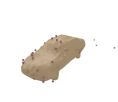
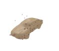
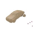
AML

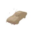
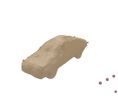
Figure 14: Comparison of AML and dAML. Our deterministic variant, dAML, suffers from inferior results. Predicted shapes in beige and observations in red at low resolution ($24\operatorname*{\!\times\!}54\operatorname*{\!\times\!}24$ voxels).

For training, we combine occupancy grids and logTSDFs in separate feature channels and randomly translate both by up to $3$ voxels per axis. Additionally, we use Bernoulli noise (probability $0.1$) and Gaussian noise (variance $0.05$). We use Adam (Kingma and Ba, 2015), a batch size of $16$ and the initialization scheme by Glorot and Bengio (2010). The shape prior is trained for $3000$ to $4000$ epochs with an initial learning rate of $10^{-4}$ which is decayed by $0.925$ every $215$ iterations until a minimum of $10^{-16}$ has been reached. In addition, weight decay ($10^{-4}$) is applied. For shape inference, training takes $30$ to $50$ epochs, and an initial learning rate of $10^{-4}$ is decayed by $0.9$ every $215$ iterations. For our learning-based baselines (see Section 4.4) we require between $300$ and $400$ epochs using the same training procedure as for the shape prior. On the Kinect dataset, where only $30$ training examples are available, we used $5000$ epochs. We use $\log\sigma^{2}=-2$ as an empirically found trade-off between accuracy of the reconstructed SDFs and ease of training – significantly lower $\log\sigma^{2}$ may lead to difficulties during training, including divergence. On ShapeNet, ModelNet and Kinect, the weight $\lambda$ of the Kullback-Leibler divergence KL (for both DVAE and (d)AML) was empirically determined to be $\lambda=2,2.5,3$ for low, medium and high resolution, respectively. On KITTI, we use $\lambda=1$ for all resolutions. In practice, $\lambda$ controls the trade-off between diversity (low $\lambda$) and quality (high $\lambda$) of the completed shapes. In addition, we reduce the weight in free space areas to one fourth on SN-noisy and KITTI to balance between occupied and free space. We implemented our networks in Torch (Collobert et al, 2011).

4.4 Baselines

Data-Driven Approaches: We consider the works by Engelmann et al (2016) and Gupta et al (2015) as data-driven baselines. Additionally, we consider regular maximum likelihood (ML). Engelmann et al (2016) – referred to as Eng16– use a principal component analysis shape prior trained on a manually selected set of car models. Shape completion is posed as optimization problem considering both shape and pose. The pre-trained shape prior provided by Engelmann et al. assumes a ground plane which is, according to KITTI’s LiDAR data, fixed at $1m$ height. Thus, we don’t need to optimize pose on KITTI as we use the ground truth bounding boxes; on ShapeNet, in contrast, we need to optimize both pose and shape to deal with the random rotations in SN-clean and SN-noisy.

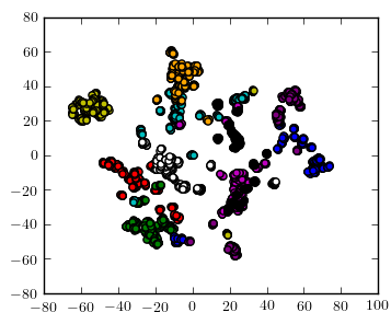
(a) DVAE t-SNE

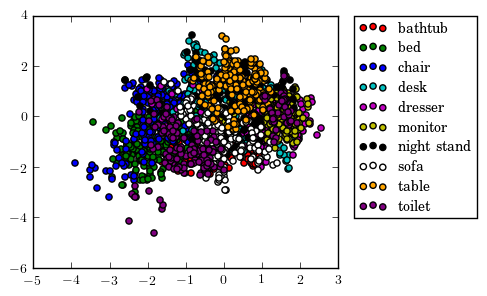
(b) DVAE Projection

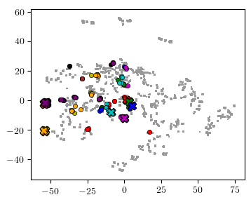
(c) AML t-SNE

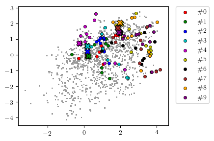
(d) AML Projection

Figure 15: Learned Latent Spaces. In (15(a)) and (15(b)), we show a t-SNE (van der Maaten and Hinton, 2008) visualization and a two-dimensional projection of the DVAE latent space on ModelNet10. The plots illustrate that the DVAE is able to separate the ten object categories. In (15(c)) and (15(d)), we show a t-SNE visualization and a projection of the latent space corresponding to our learned AML model on SN-clean. We randomly picked $10$ ground truth shapes, “x”, and the corresponding observations ($10$ per shape), points (gray pixels indicate remaining shapes/observations). The plots illustrate that AML is able to associate observations with the corresponding ground truth shapes under weak supervision.

Supervision	Method	SN-clean				SN-noisy				KITTI
in %		Ham$\downarrow$	IoU$\uparrow$	Acc [vx] $\downarrow$	Comp [vx] $\downarrow$	Ham$\downarrow$	IoU$\uparrow$	Acc [vx] $\downarrow$	Comp [vx] $\downarrow$	Comp [m] $\downarrow$
Low Resolution: $24\times 54\times 24$ voxels; * independent of resolution
(shape prior)	DVAE	0.019	0.885	0.283	0.527	(same shape prior as on SN-clean)
$\hphantom{<}100$	Dai et al (2017) (Dai17)	0.021	0.872	0.321	0.564	0.027	0.836	0.391	0.633	0.128
	Sup	0.026	0.841	0.409	0.607	0.028	0.833	0.407	0.637	0.091
$<7.7$	Naïve	0.067	0.596	0.999	1.335	0.064	0.609	0.941	1.29	–
	Mean	0.052	0.697	0.79	0.938	0.052	0.696	0.79	0.938	–
	ML	0.04	0.756	0.637	0.8	0.041	0.755	0.625	0.829	(too slow)
	*Gupta et al (2015) (ICP)	(mesh only)		0.534	0.503	(mesh only)		7.551	6.372	(too slow)
	*Engelmann et al (2016) (Eng16)	(mesh only)		1.235	1.237	(mesh only)		1.974	1.312	0.13
	dAML	0.034	0.784	0.532	0.741	0.036	0.772	0.557	0.76	(see AML)
	AML	0.034	0.779	0.549	0.753	0.036	0.771	0.57	0.761	0.12
Low Resolution: $24\times 54\times 24$ voxels; Multiple, $k>1$ Fused Views
$\hphantom{<}100$	Dai et al (2017) (Dai17), $k=5$	0.012	0.924	0.214	0.436	0.018	0.887	0.278	0.491	n/a
	Sup, $k=5$	0.022	0.866	0.336	0.566	0.024	0.86	0.331	0.573
$<16$	AML, $k=2$	0.032	0.794	0.489	0.695	0.034	0.79	0.52	0.725	n/a
$<24$	AML, $k=3$	0.031	0.809	0.471	0.667	0.031	0.81	0.493	0.67
$<40$	AML, $k=5$	0.031	0.804	0.502	0.686	0.035	0.799	0.523	0.7
Medium Resolution: $32\times 72\times 32$ voxels
(shape prior)	DVAE	0.019	0.877	0.24	0.47	(same shape prior as on SN-clean)
$\hphantom{<}100$	Dai et al (2017) (Dai17)	0.02	0.869	0.399	0.674	0.026	0.83	0.51	0.767	0.074
	Sup	0.027	0.834	0.498	0.789	0.029	0.815	0.571	0.843	0.09
$\leq 6.1$	AML	0.031	0.788	0.415	0.584	0.036	0.766	0.721	0.953	0.083
High Resolution: $48\times 108\times 48$ voxels
(shape prior)	DVAE	0.018	0.87	0.272	0.434	(same shape prior as on SN-clean)
$\hphantom{<}100$	Dai17	0.017	0.88	0.517	0.827	0.054	0.664	1.559	2.067	0.066
	Sup	0.023	0.843	0.677	1.032	0.052	0.674	1.52	1.981	0.091
$<3.5$	AML	0.028	0.796	0.433	0.579	0.045	0.659	1.4	1.957	0.078

Table 2: Quantitative Results on ShapeNet and KITTI. We consider Hamming distance (Ham) and intersection over union (IoU) for occupancy grids as well as accuracy (Acc) and completeness (Comp) for meshes on SN-clean, SN-noisy and KITTI. For Ham, Acc and Comp, lower is better; for IoU, higher is better. The unit of Acc and Comp is voxels (voxel length at $24\operatorname*{\!\times\!}54\operatorname*{\!\times\!}48$ voxels) or meters. Note that the DVAE shape prior (in gray) is only reported as reference (i.e., bound on (d)AML). We indicate the level of supervision in percentage, relative to the corresponding resolution (see Table 1) and mark the best results under full supervision in red and under weak supervision in green.

Inspired by the work by Gupta et al (2015) we also consider a shape retrieval and fitting baseline. Specifically, we perform iterative closest point (ICP) (Besl and McKay, 1992) fitting on all training shapes and subsequently select the best-fitting one. To this end, we uniformly sample $1\text{Mio}$ points on the training shapes, and perform point-to-point ICP for a maximum of $100$ iterations using $\left[\begin{matrix}R&t\end{matrix}\right]=\left[\begin{matrix}I_{3}&0\end{matrix}\right]$ as initialization. On the training set, we verified that this approach is always able to retrieve the perfect shape.

Finally, we consider a simple ML baseline iteratively minimizing Eq. (7) using stochastic gradient descent (SGD). This baseline is similar to the work by Engelmann et al., however, like ours it is bound to the voxel grid. Per example, we allow a maximum of $5000$ iterations, starting with latent code $z=0$, learning rate $0.05$ and momentum $0.5$ (decayed every $50$ iterations at rate $0.85$ and $1.0$ until $10^{-5}$ and $0.9$ have been reached).

Learning-Based Approaches: Learning-based approaches usually employ an encoder-decoder architecture to directly learn a mapping from observations $x_{n}$ to ground truth shapes $y_{n}^{*}$ in a fully supervised setting (Wang et al, 2017; Varley et al, 2017; Yang et al, 2018, 2017; Dai et al, 2017). While existing architectures differ slightly, they usually rely on a U-net architecture (Ronneberger et al, 2015; Cicek et al, 2016). In this paper, we use the approach of Dai et al (2017) – referred to as Dai17– as a representative baseline for this class of approaches. In addition, we consider a custom learning-based baseline which uses the architecture of our DVAE shape prior, cf. Fig. 11. In contrast to (Dai et al, 2017), this baseline is also limited by the low-dimensional ($Q=10$) bottleneck as it does not use skip connections.

Obs

Dai17

Dai17

Eng16

ML

ML

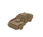
AML

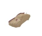
AML

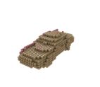
GT

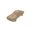
GT

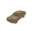
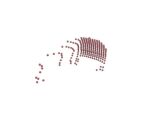
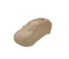
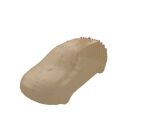
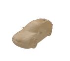
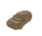
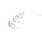
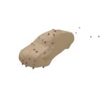
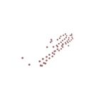
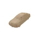
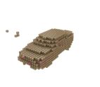
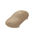
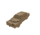
(a) SN-clean (Top) and SN-noisy (Bottom), Low Resolution ($24\operatorname*{\!\times\!}54\operatorname*{\!\times\!}24$)

Obs

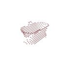
Dai17

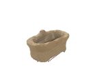
Dai17

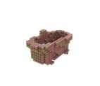
ICP

ML

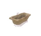
ML

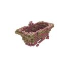
AML

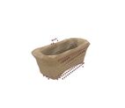
AML

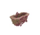
GT

GT

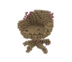
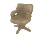
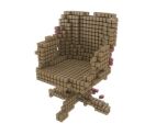
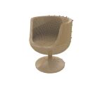
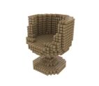
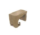
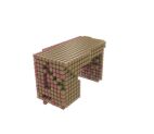
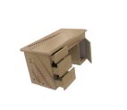
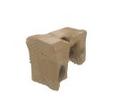
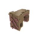
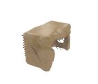
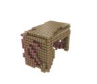
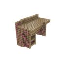
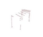
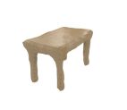
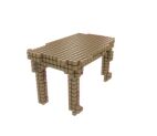
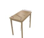
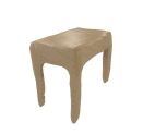
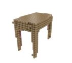
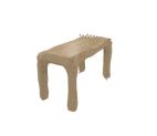
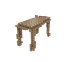
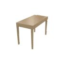
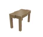
(b) ModelNet Bathtubs, Chairs, Desks and Tables, Low Resolution ($32^{3}$)

Figure 17: Qualitative Results on ShapeNet and ModelNet. Results for AML, Dai17, Eng16, ICP and ML on SN-clean, SN-noisy and ModelNet’s bathtubs, chairs, desks and tables. AML outperforms data-driven approaches (ML, Eng16, ICP) and rivals Dai17 while requiring significantly less supervision. Occupancy grids and meshes in beige, observations in red.

Supervision	Method	bathtub		chair				desk		table		ModelNet10
in %		Ham$\downarrow$	IoU$\uparrow$	Ham$\downarrow$	IoU$\uparrow$	Acc [vx]$\downarrow$	Comp [vx]$\downarrow$	Ham$\downarrow$	IoU$\uparrow$	Ham$\downarrow$	IoU$\uparrow$	Ham$\downarrow$	IoU$\uparrow$
Low Resolution: $32^{3}$ voxels; * independent of resolution
(shape prior)	DVAE	0.015	0.699	0.025	0.517	0.884	0.72	0.028	0.555	011	0.608	0.023	0.714
$\hphantom{<}100$	Dai et al (2017) (Dai17)	0.022	0.59	0.019	0.61	0.663	0.671	0.027	0.568	0.011	0.648	0.03	0.646
	Sup	0.023	0.618	0.03	0.478	0.873	0.813	0.036	0.458	0.017	0.497	0.038	0.589
$<10$	* Gupta et al (2015) (ICP)	(mesh only)		(mesh only)		1.483	0.89	(mesh only)		(mesh only)		(mesh only)
	ML	0.028	0.503	0.033	0.414	1.489	1.065	0.048	0.323	0.029	0.318	(too slow)
	AML	0.026	0.503	0.033	0.373	1.088	0.785	0.041	0.389	0.018	0.423	0.04	0.509
Medium Resolution: $48^{3}$ voxels
(shape prior)	DVAE	0.014	0.671	0.021	0.491	0.748	0.697	0.025	0.525	0.01	0.548
$\hphantom{<}100$	Dai et al (2017) (Dai17)	0.018	0.609	0.016	0.576	0.513	0.508	0.023	0.532	0.008	0.65
$<9$	AML	0.024	0.459	0.029	0.347	1.025	0.805	0.034	0.361	0.015	0.384
High Resolution: $64^{3}$ voxels
(shape prior)	DVAE	0.014	0.644	0.02	0.474	0.702	0.705	0.024	0.506	0.009	0.548
$\hphantom{<}100$	Dai et al (2017) (Dai17)	0.018	0.54	0.016	0.548	0.47	0.53	0.021	0.525	0.007	0.673
$<9$	AML	0.023	0.46	0.026	0.333	0.893	0.852	0.042	0.31	0.012	0.407

Table 3: Quantitative Results on ModelNet. Results for bathtubs, chairs, desks, tables and all ten categories combined (ModelNet10). As the ground truth SDFs are merely approximations (cf. Section 4.1), we concentrate on Hamming distance (Ham; lower is better) and intersection-over-union (IoU; higher is better). Only for chairs, we report accuracy Acc and completeness Comp in voxels (voxel length at $32^{3}$ voxels). We also indicate the level of supervision (see Table 1). Again, we report the DVAE shape prior as reference and color the best weakly-supervised approach using green and the best fully-supervised approach in red.

$k=3$

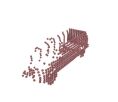
AML

GT

$k=5$

AML

GT

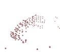
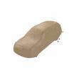
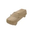
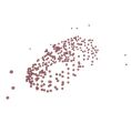
(a) SN-clean and -noisy, $k$ Views, Low Resolution ($24\operatorname*{\!\times\!}54\operatorname*{\!\times\!}24$)

Dai17

AML

GT

Dai17

AML

GT

(b) SN-clean and -noisy, Medium ($32\operatorname*{\!\times\!}72\operatorname*{\!\times\!}32$) and High ($48\operatorname*{\!\times\!}108\operatorname*{\!\times\!}48$) Resolution

Dai17

AML

GT

Dai17

AML

GT

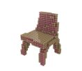
(c) ModelNet desks and chairs, Medium ($48^{3}$) and High ($64^{3}$) Resolution

Figure 19: Multi-View and Higher-Resolution Results on ShapeNet and ModelNet. While AML is designed for especially sparse observations, it also performs well in a multi-view setting. Additionally, higher resolutions allow to predict more detailed shapes. Shapes, occupancy grids or meshes, in beige and observations in red.

Dai17

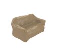
AML

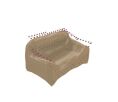
GT

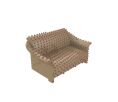
Dai17

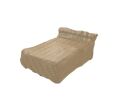
AML

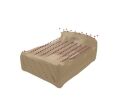
GT

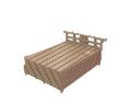
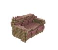
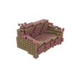
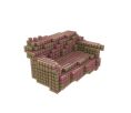
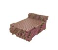
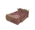
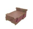
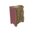
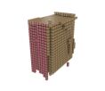
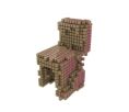
Figure 20: Category-Agnostic Results on ModelNet10. AML is able to recover detailed shapes of the correct object category even without category supervision (as provided to Dai17). Shapes (occupancy grids and meshes) in beige and observations in red at low resolution ($32^{3}$ voxels).

Obs

Dai17

Eng16

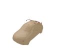
AML

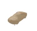
AML

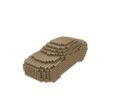
GT

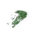
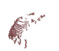
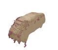
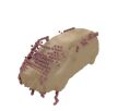
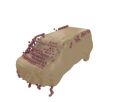
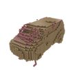
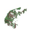
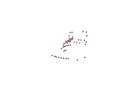
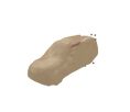
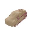
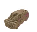
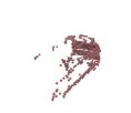
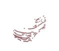
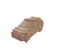
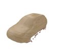
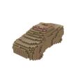
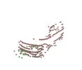
(a) KITTI, Medium Resolution ($32\operatorname*{\!\times\!}72\operatorname*{\!\times\!}32$)

Obs

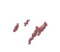
AML

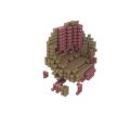
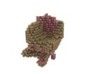
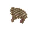
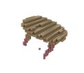
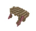
(b) Kinect, Low Resolution ($32^{3}$)

Figure 22: Qualitative Results on KITTI and Kinect. On KITTI, AML visually outperforms both Dai17 and Eng16 while being faster and requiring less supervision. On Kinect, AML demonstrates that it is able to generalize from as few as $30$ training samples. Predicted shapes (occupancy grids or meshes) in beige and observations in red; additionally, partial ground truth in green.

AML

GT

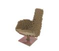
AML

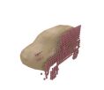
GT

AML

Dai17

Dai17

(a) Difficulties with Exotic Shapes and Fine Structures

Dai17

AML

GT

Dai17

AML

GT

(b) Difficulties with Multiple Object Categories

Figure 24: Failures Cases. On the top, we show that AML has difficulties with exotic shapes, not represented in the latent space; and both AML and Dai17 have difficulties with fine details. The bottom row demonstrates that it is difficult to infer the correct object category from sparse observations, even under full supervision as required by Dai17. Shapes (occupancy grids and mehses) in beige and observations in red from various resolutions.

4.5 Experimental Evaluation

Quantitative results are summarized in Table 2 (ShapeNet and KITTI) and 3 (ModelNet). Qualitative results for the shape prior are shown in Fig. 14 and 15; shape completion results are shown in Fig. 17 (ShapeNet and ModelNet) and 22 (KITTI and Kinect).

Latent Space Dimensionality: Regarding our DVAE shape prior, we found the dimensionality $Q$ to be of crucial importance as it defines the trade-off between reconstruction accuracy and random sample quality (i.e., the quality of the generative model). A higher-dimension-al latent space usually results in higher-quality reconstructions but also imposes the difficulty of randomly generating meaningful shapes. Across all datasets, we found $Q=10$ to be suitable – which is significantly smaller compared to related work: $35$ in (Liu et al, 2017), $6912$ in (Sharma et al, 2016), $200$ for (Wu et al, 2016b; Smith and Meger, 2017) or $64$ in (Girdhar et al, 2016). Still, we are able to obtain visually appealing results. Finally, in Fig. 14 we show qualitative results, illustrating good reconstruction performance and reasonable random samples across resolutions.

Fig. 15 shows a t-SNE (van der Maaten and Hinton, 2008) visualization as well as a projection of the $Q=10$ dimensional latent space, color coding the $10$ object categories of ModelNet10. The DVAE clusters the object categories within the support region of the unit Gaussian. In the t-SNE visualization, we additionally see ambiguities arising in ModelNet10, e.g., night stands and dressers often look indistinguishable while monitors are very dissimilar to all other categories. Overall, these findings support our decision to use a DVAE with $Q=10$ as shape prior.

Ablation Study: In Table 2, we show quantitative results of our model on SN-clean and SN-noisy. First, we report the reconstruction quality of the DVAE shape prior as reference. Then, we consider the DVAE shape prior (Naïve), and its mean prediction (Mean) as simple baselines. The poor performance of both illustrates the difficulty of the benchmark. For AML, we also consider its deterministic variant, dAML (see Section 3). Quantitatively, there is essentially no difference; however, Fig. 14 demonstrates that AML is able to predict more detailed shapes. We also found that using both occupancy and SDFs is necessary to obtain good performance – as is using both point observations and free space.

Considering Fig. 15, we additionally demonstrate that the embedding learned by AML, i.e., the embedding of incomplete observations within the latent shape space, is able to associate observations with corresponding shapes even under weak supervision. In particular, we show a t-SNE visualization and a projection of the latent space for AML trained on SN-clean. We color-code $10$ randomly chosen ground truth shapes, resulting in $100$ observations ($10$ views per shape). AML is usually able to embed observations near the corresponding ground truth shapes, without explicit supervision (e.g., for violet, pink, blue or teal, the observations – points – are close to the corresponding ground truth shapes – “x”). Additionally, AML also matches the unit Gaussian prior distribution reasonably well.

Comparison to Baselines on Synthetic Data: For ShapeNet, Table 2 demonstrates that AML outperforms data-driven approaches such as Eng16, ICP and ML and is able to compete with fully-supervised approaches, Dai17 and Sup, while using only $8\%$ or less supervision. We also note that AML outperforms ML, illustrating that amortized inference is beneficial. Furthermore, Dai17 outperforms Sup, illustrating the advantage of propagating low-level information (through skip connections) without bottleneck. Most importantly, the performance gap between AML and Dai17 is rather small considering the difference in supervision (more than $92\%$) and on SN-noisy, the drop in performance for Dai17 and Sup is larger than for AML suggesting that AML handles noise and sparsity more robustly. Fig. 17 shows that these conclusions also apply visually where AML performs en par with Dai17.

For ModelNet, in Table 3, we mostly focus on occupancy grids (as the derived SDFs are approximate, cf. Section 4.1) and show that chairs, desks or tables are more difficult. However, AML is still able to predict high-quality shapes, outperforming data-driven approaches. Additionally, in comparison to ShapeNet, the gap between AML and fully-supervised approaches (Dai17 and Sup) is surprisingly small – not reflecting the difference in supervision. This means that even under full supervision, these object categories are difficult to complete. In terms of accuracy (Acc) and completeness (Comp), e.g., for chairs, AML outperforms ICP and ML; Dai17 and Sup, on the other hand, outperform AML. Still, considering Fig. 17, AML predicts visually appealing meshes although the reference shape SDFs on ModelNet are merely approximate. Qualitatively, AML also outperforms its data-driven rivals; only Dai17 predicts shapes slightly closer to the ground truth.

Multiple Views and Higher Resolutions: In Table 2, we consider multiple, $k\in\{2,3,5\}$, randomly fused observations (from the $10$ views per shape). Generally, additional observations are beneficial (also cf. Fig. 19); however, fully-supervised approaches such as Dai17 benefit more significantly than AML. Intuitively, especially on SN-noisy, $k=5$ noisy observations seem to impose contradictory constraints that cannot be resolved under weak supervision. We also show that higher resolution allows both AML and Dai17 to predict more detailed shapes, see Fig. 19; for AML this is significant as, e.g., on SN-noisy, the level of supervision reduces to less than $1\%$. Also note that AML is able to handle the slightly asymmetric desks in Fig. 19 due to the strong shape prior which itself includes symmetric and less symmetric shapes.

Multiple Object Categories: We also investigate the category-agnostic case, considering all ten ModelNet10 object categories; here, we train a single DVAE shape prior (as well as a single model for Dai17 and Sup) across all ten object categories. As can be seen in Table 3, the gap between AML and fully-supervised approaches, Dai17 and Sup, further shrinks; even fully-supervised methods have difficulties distinguishing object categories based on sparse observations. Fig. 19 shows that AML is able to not only predict reasonable shapes, but also identify the correct object category. In contrast to Dai17, which predicts slightly more detailed shapes, this is significant as AML does not have access to object category information during training.

Comparison on Real Data: On KITTI, considering Fig. 22, we illustrate that AML consistently predicts detailed shapes regardless of the noise and sparsity in the inputs. Our qualitative results suggest that AML is able to predict more detailed shapes compared to Dai17 and Eng16; additionally, Eng16 is distracted by sparse and noisy observations. Quantitatively, instead, Dai17 and Sup outperform AML. However, this is mainly due to two factors: first, the ground truth collected on KITTI does rarely cover the full car; and second, we put significant effort into faithfully modeling KITTI’s noise statistics in SN-noisy, allowing Dai17 and Sup to generalize very well. The latter effort, especially, can be avoided by using our weakly-supervised approach, AML.

On Kinect, also considering Fig. 22, only $30$ observations are available for training. It can be seen that AML predicts reasonable shapes for tables. We find it interesting that AML is able to generalize from only $30$ training examples. In this sense, AML functions similar to ML, in that the objective is trained to overfit to few samples. This, however, cannot work in all cases, as demonstrated by the chairs where AML tries to predict a suitable chair, but does not fit the observations as well. Another problem witnessed on Kinect, is that the shape prior training samples need to be aligned to the observations (with respect to the viewing angles). For the chairs, we were not able to guess the viewing trajectory correctly (cf. (Yang et al, 2018)).

Failure Cases: AML and Dai17 often face similar problems, as illustrated in Fig. 24, suggesting that these problems are inherent to the used shape representations or the learning approach independent of the level of supervision. For example, both AML and Dai17 have problems with fine, thin structures that are hard to reconstruct properly at any resolution. Furthermore, identifying the correct object category on ModelNet10 from sparse observations is difficult for both AML and Sup. Finally, AML additionally has difficulties with exotic objects that are not well represented in the latent shape space as, e.g., designed chairs.

Runtime: At low resolution, AML as well as the fully-supervised approaches Dai17 and Sup, are particular fast, requiring up to $2ms$ on a NVIDIA™ GeForce® GTX TITAN using Torch (Collobert et al, 2011). Data-driven approaches (e.g., Eng16, ICP and ML), on the other hand, take considerably longer. Eng16, for instance requires $168ms$ on average for completing the shape of a sparse LIDAR observation from KITTI using an Intel® Xeon® E5-2690 @2.6Ghz and the multi-threaded Ceres solver (Agarwal et al, 2012). ICP and ML take longest, requiring up to $38s$ and $75s$ (not taking into account the point sampling process for the shapes), respectively. Except for Eng16 and ICP, all approaches scale with the used resolution and the employed architecture.

5 Conclusion

In this paper, we presented a novel, weakly-supervised learning-based approach to 3D shape completion from sparse and noisy point cloud observations. We used a (denoising) variational auto-encoder (Im et al, 2017; Kingma and Welling, 2014) to learn a latent space of shapes for one or multiple object categories using synthetic data from ShapeNet (Chang et al, 2015) or ModelNet (Wu et al, 2015). Based on the learned generative model, i.e., decoder, we formulated 3D shape completion as a maximum likelihood problem. In a second step, we then fixed the learned generative model and trained a new recognition model, i.e. encoder, to amortize, i.e. learn, the maximum likelihood problem. Thus, our Amortized Maximum Likelihood (AML) approach to 3D shape completion can be trained in a weakly-supervised fashion. Compared to related data-driven approaches, e.g., (Rock et al, 2015; Haene et al, 2014; Li et al, 2015; Engelmann et al, 2016, 2017; Nan et al, 2012; Bao et al, 2013; Dame et al, 2013; Nguyen et al, 2016), our approach offers fast inference at test time; in contrast to other learning-based approaches, e.g., (Riegler et al, 2017a; Smith and Meger, 2017; Dai et al, 2017; Sharma et al, 2016; Fan et al, 2017; Rezende et al, 2016; Yang et al, 2018; Wang et al, 2017; Varley et al, 2017; Han et al, 2017), we do not require full supervision during training. Both characteristics render our approach useful for robotic scenarios where full supervision is often not available such as in autonomous driving, e.g., on KITTI (Geiger et al, 2012), or indoor robotics, e.g., on Kinect (Yang et al, 2018).

On two newly created synthetic shape completion benchmarks, derived from ShapeNet’s cars and ModelNet10, as well as on real data from KITTI and, we demonstrated that AML outperforms related data-driven approaches (Engelmann et al, 2016; Gupta et al, 2015) while being significantly faster. We further showed that AML is able to compete with fully-supervised approaches (Dai et al, 2017), both quantitatively and qualitatively, while using only $3-10\%$ supervision or less. In contrast to (Rock et al, 2015; Haene et al, 2014; Li et al, 2015; Engelmann et al, 2016, 2017; Nan et al, 2012; Bao et al, 2013; Dame et al, 2013), we additionally showed that AML is able to generalize across object categories without category supervision during training. On Kinect, we also demonstrated that our AML approach is able to generalize from very few training examples. In contrast to (Girdhar et al, 2016; Liu et al, 2017; Sharma et al, 2016; Wu et al, 2015; Dai et al, 2017; Firman et al, 2016; Han et al, 2017; Fan et al, 2017), we considered resolutions up to $48\operatorname*{\!\times\!}108\operatorname*{\!\times\!}48$ and $64^{3}$ voxels as well as significantly sparser observations. Overall, our experiments demonstrate two key advantages of the proposed approach: significantly reduced runtime and increased performance compared to data-driven approaches showing that amortizing inference is highly effective.

In future work, we would like to address several aspects of our AML approach. First, the shape prior is essential for weakly-supervised shape completion, as also noted by Gwak et al (2017). However, training expressive generative models in 3D is still difficult. Second, larger resolutions imply significantly longer training times; alternative shape representations and data structures such as point clouds (Qi et al, 2017a, b; Fan et al, 2017) or octrees (Riegler et al, 2017b, a; Häne et al, 2017) might be beneficial. Finally, jointly tackling pose estimation and shape completion seems promising (Engelmann et al, 2016).

References

- Abramowitz (1974) Abramowitz M (1974) Handbook of Mathematical Functions, With Formulas, Graphs, and Mathematical Tables. Dover Publications
- Agarwal et al (2012) Agarwal S, Mierle K, Others (2012) Ceres solver. http://ceres-solver.org
- Aubry et al (2014) Aubry M, Maturana D, Efros A, Russell B, Sivic J (2014) Seeing 3D chairs: exemplar part-based 2D-3D alignment using a large dataset of CAD models. In: Proc. IEEE Conf. on Computer Vision and Pattern Recognition (CVPR)
- Bao et al (2013) Bao S, Chandraker M, Lin Y, Savarese S (2013) Dense object reconstruction with semantic priors. In: Proc. IEEE Conf. on Computer Vision and Pattern Recognition (CVPR)
- Besl and McKay (1992) Besl P, McKay H (1992) A method for registration of 3d shapes. IEEE Trans on Pattern Analysis and Machine Intelligence (PAMI) 14:239–256
- Blei et al (2016) Blei DM, Kucukelbir A, McAuliffe JD (2016) Variational inference: A review for statisticians. arXivorg 1601.00670
- Brock et al (2016) Brock A, Lim T, Ritchie JM, Weston N (2016) Generative and discriminative voxel modeling with convolutional neural networks. arXivorg 1608.04236
- Chang et al (2015) Chang AX, Funkhouser TA, Guibas LJ, Hanrahan P, Huang Q, Li Z, Savarese S, Savva M, Song S, Su H, Xiao J, Yi L, Yu F (2015) Shapenet: An information-rich 3d model repository. arXivorg 1512.03012
- Chen et al (2016) Chen X, Kundu K, Zhu Y, Ma H, Fidler S, Urtasun R (2016) 3d object proposals using stereo imagery for accurate object class detection. arXivorg 1608.07711
- Choy et al (2016) Choy CB, Xu D, Gwak J, Chen K, Savarese S (2016) 3d-r2n2: A unified approach for single and multi-view 3d object reconstruction. In: Proc. of the European Conf. on Computer Vision (ECCV)
- Cicek et al (2016) Cicek Ö, Abdulkadir A, Lienkamp SS, Brox T, Ronneberger O (2016) 3d u-net: Learning dense volumetric segmentation from sparse annotation. arXivorg 1606.06650
- Cignoni et al (2008) Cignoni P, Callieri M, Corsini M, Dellepiane M, Ganovelli F, Ranzuglia G (2008) Meshlab: an open-source mesh processing tool
- Collobert et al (2011) Collobert R, Kavukcuoglu K, Farabet C (2011) Torch7: A matlab-like environment for machine learning. In: Advances in Neural Information Processing Systems (NIPS) Workshops
- Curless and Levoy (1996) Curless B, Levoy M (1996) A volumetric method for building complex models from range images. In: ACM Trans. on Graphics (SIGGRAPH)
- Dai et al (2017) Dai A, Qi CR, Nießner M (2017) Shape completion using 3d-encoder-predictor cnns and shape synthesis. In: Proc. IEEE Conf. on Computer Vision and Pattern Recognition (CVPR)
- Dame et al (2013) Dame A, Prisacariu V, Ren C, Reid I (2013) Dense reconstruction using 3D object shape priors. In: Proc. IEEE Conf. on Computer Vision and Pattern Recognition (CVPR)
- Eigen and Fergus (2015) Eigen D, Fergus R (2015) Predicting depth, surface normals and semantic labels with a common multi-scale convolutional architecture. In: Proc. of the IEEE International Conf. on Computer Vision (ICCV)
- Eigen et al (2014) Eigen D, Puhrsch C, Fergus R (2014) Depth map prediction from a single image using a multi-scale deep network. In: Advances in Neural Information Processing Systems (NIPS)