Sequential Learning of Principal Curves: Summarizing Data Streams on the Fly

Abstract

When confronted with massive data streams, summarizing data with dimension reduction methods such as PCA raises theoretical and algorithmic pitfalls. Principal curves act as a nonlinear generalization of PCA and the present paper proposes a novel algorithm to automatically and sequentially learn principal curves from data streams. We show that our procedure is supported by regret bounds with optimal sublinear remainder terms. A greedy local search implementation (called slpc, for Sequential Learning Principal Curves) that incorporates both sleeping experts and multi-armed bandit ingredients is presented, along with its regret computation and performance on synthetic and real-life data.

Keywords

sequential learning, principal curves, data streams, regret bounds, greedy algorithm, sleeping experts. MSC 2010: 68T10, 62L10, 62C99.

1 Introduction

Numerous methods have been proposed in the statistics and machine learning literature to sum up information and represent data by condensed and simpler-to-understand quantities. Among those methods, Principal Component Analysis (PCA) aims at identifying the maximal variance axes of data. This serves as a way to represent data in a more compact fashion and hopefully reveal as well as possible their variability. PCA has been introduced by Pearson (1901) and Spearman (1904) and further developed by Hotelling (1933). This is one of the most widely used procedures in multivariate exploratory analysis targeting dimension reduction or features extraction. Nonetheless, PCA is a linear procedure and the need for more sophisticated nonlinear techniques has led to the notion of principal curve. Principal curves may be seen as a nonlinear generalization of the first principal component. The goal is to obtain a curve which passes "in the middle" of data, as illustrated by Figure 1. This notion of skeletonization of data clouds has been at the heart of numerous applications in many different domains, such as physics (Friedsam and Oren, 1989; Brunsdon, 2007), character and speech recognition (Reinhard and Niranjan, 1999; Kégl and Krzyżak, 2002), mapping and geology (Banfield and Raftery, 1992; Stanford and Raftery, 2000; Brunsdon, 2007), to name but a few.

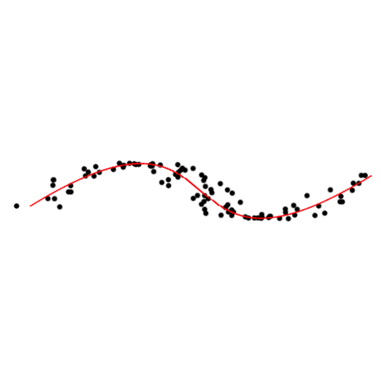
Figure 1: A principal curve.

1.1 Earlier works on principal curves

The original definition of principal curve dates back to Hastie and Stuetzle (1989). A principal curve is a smooth ($C^{\infty}$) parameterized curve $\mathbf{f}(s)=\left(f_{1}(s),\dots,f_{d}(s)\right)$ in $\mathbb{R}^{d}$ which does not intersect itself, has finite length inside any bounded subset of $\mathbb{R}^{d}$ and is self-consistent. This last requirement means that $\mathbf{f}(s)=\mathbb{E}[X|s_{\mathbf{f}}(X)=s]$, where $X\in\mathbb{R}^{d}$ is a random vector and the so-called projection index $s_{\mathbf{f}}(x)$ is the largest real number $s$ minimizing the squared Euclidean distance between $\mathbf{f}(s)$ and $x$, defined by

$$s_{\mathbf{f}}(x)=\sup\left\{s:\left\|x-\mathbf{f}(s)\right\|_{2}^{2}=\inf_{\tau}\ \left\|x-\mathbf{f}(\tau)\right\|_{2}^{2}\right\}.$$

Self-consistency means that each point of $\mathbf{f}$ is the average (under the distribution of $X$) of all data points projected on $\mathbf{f}$, as illustrated by Figure 2.

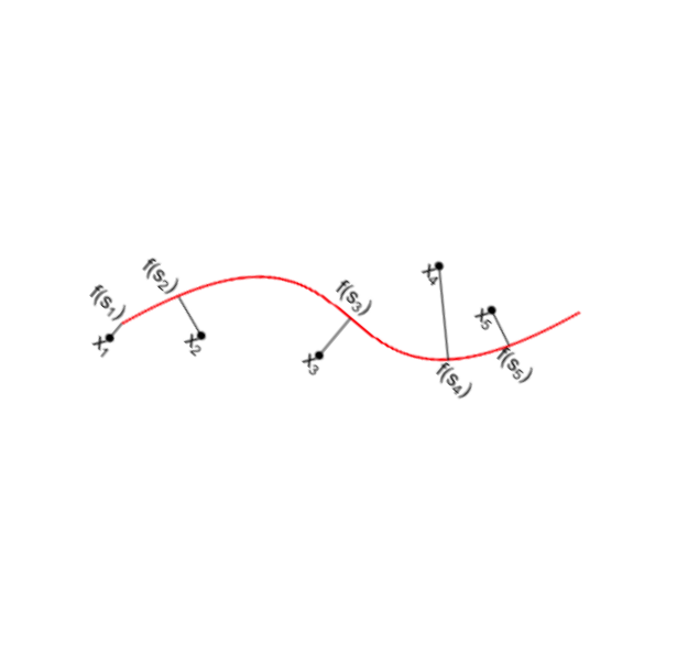
Figure 2: A principal curve and projections of data onto it.

However, an unfortunate consequence of this definition is that the existence is not guaranteed in general for a particular distribution, let alone for an online sequence for which no probabilistic assumption is made. Kégl (1999) proposed a new concept of principal curves which ensures its existence for a large class of distributions. Principal curves $\mathbf{f}^{\star}$ are defined as the curves minimizing the expected squared distance over a class $\mathcal{F}_{L}$ of curves whose length is smaller than $L>0$, namely,

$$\mathbf{f}^{\star}\in\underset{\mathbf{f}\in\mathcal{F}_{L}}{\arg\inf}\ \Delta(\mathbf{f}),$$

where

$$\Delta(\mathbf{f})=\mathbb{E}\left[\Delta\left(\mathbf{f},X\right)\right]=\mathbb{E}\left[\inf_{s}\ \left\|\mathbf{f}(s)-X\right\|_{2}^{2}\right].$$

If $\mathbb{E}\|X\|_{2}^{2}<\infty$, $\mathbf{f}^{\star}$ always exists but may not be unique. In practical situation where only i.i.d copies $X_{1},\dots,X_{n}$ of $X$ are observed, Kégl (1999) considers classes $\mathcal{F}_{k,L}$ of all polygonal lines with $k$ segments and length not exceeding $L$, and chooses an estimator $\hat{\mathbf{f}}_{k,n}$ of $\mathbf{f}^{\star}$ as the one within $\mathcal{F}_{k,L}$ which minimizes the empirical counterpart

$$\Delta_{n}(\mathbf{f})=\frac{1}{n}\sum_{i=1}^{n}\Delta\left(\mathbf{f},X_{i}\right)$$

of $\Delta(\mathbf{f})$. It is proved in Kégl et al. (2000) that if $X$ is almost surely bounded and $k\propto n^{1/3}$, then

$$\Delta\left(\hat{\mathbf{f}}_{k,n}\right)-\Delta\left(\mathbf{f}^{\star}\right)=\mathcal{O}\left(n^{-1/3}\right).$$

As the task of finding a polygonal line with $k$ segments and length at most $L$ that minimizes $\Delta_{n}(\mathbf{f})$ is computationally costly, Kégl et al. (2000) proposes the Polygonal Line algorithm. This iterative algorithm proceeds by fitting a polygonal line with $k$ segments and considerably speeds up the exploration part by resorting to gradient descent. The two steps (projection and optimization) are similar to what is done by the $k$-means algorithm. However, the Polygonal Line algorithm is not supported by theoretical bounds and leads to variable performance depending on the distribution of the observations.

As the number $k$ of segments plays a crucial role (a too small $k$ leads to a poor summary of data while a too large $k$ yields overfitting, see Figure 3), Biau and Fischer (2012) aim to fill the gap by selecting an optimal $k$ from both theoretical and practical perspectives.

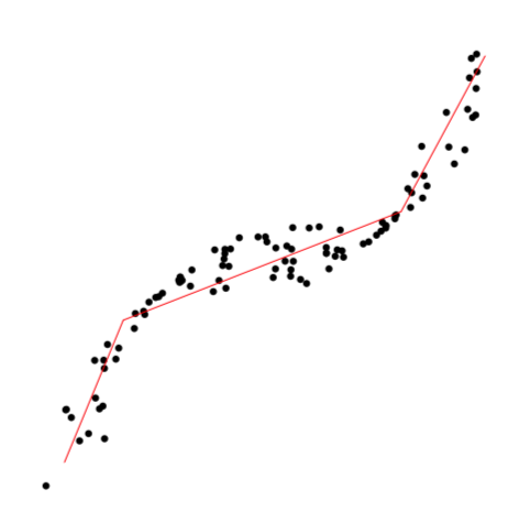
(a) A too small $k$.

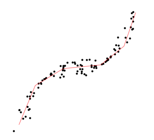
(b) Right $k$.

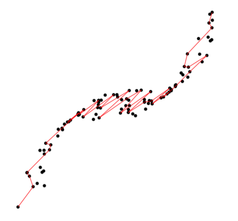
(c) A too large $k$.

Figure 3: Principal curves with different number $k$ of segments.

Their approach relies strongly on the theory of model selection by penalization introduced by Barron et al. (1999) and further developed by Birgé and Massart (2007). By considering countable classes $\{\mathcal{F}_{k,\ell}\}_{k,\ell}$ of polygonal lines with $k$ segments, total length $\ell\leq L$ and whose vertices are on a lattice, the optimal $(\hat{k},\hat{\ell})$ is obtained as the minimizer of the criterion

$$\text{crit}(k,\ell)=\Delta_{n}\left(\hat{\mathbf{f}}_{k,\ell}\right)+\text{pen}(k,\ell),$$

where

$$\text{pen}(k,\ell)=c_{0}\sqrt{\frac{k}{n}}+c_{1}\frac{\ell}{n}+c_{2}\frac{1}{\sqrt{n}}+\delta^{2}\sqrt{\frac{w_{k,\ell}}{2n}}$$

is a penalty function where $\delta$ stands for the diameter of observations, $w_{k,\ell}$ denotes the weight attached to class $\mathcal{F}_{k,\ell}$ and with constants $c_{0},c_{1},c_{2}$ depending on $\delta$, the maximum length $L$ and the dimension of observations. Biau and Fischer (2012) then prove that

$$\mathbb{E}\left[\Delta(\hat{\mathbf{f}}_{\hat{k},\hat{\ell}})-\Delta(\mathbf{f}^{\star})\right]\leq\inf_{k,\ell}\ \Big{\{}\mathbb{E}\left[\Delta(\hat{\mathbf{f}}_{k,\ell})-\Delta(\mathbf{f}^{\star})\right]+\text{pen}(k,\ell)\Big{\}}+\frac{\delta^{2}\Sigma}{2^{3/2}}\sqrt{\frac{\pi}{n}},$$ (1)

where $\Sigma$ is a numerical constant. The expected loss of the final polygonal line $\hat{\mathbf{f}}_{\hat{k},\hat{\ell}}$ is close to the minimal loss achievable over $\mathcal{F}_{k,\ell}$ up to a remainder term decaying as $1/\sqrt{n}$.

1.2 Motivation

The big data paradigm—where collecting, storing and analyzing massive amounts of large and complex data becomes the new standard—commands to revisit some of the classical statistical and machine learning techniques. The tremendous improvements of data acquisition infrastructures generates new continuous streams of data, rather than batch datasets. This has drawn a large interest to sequential learning. Extending the notion of principal curves to the sequential settings opens immediate practical application possibilities. As an example, path planning for passengers’ location can help taxi companies to better optimize their fleet. Online algorithms that could yield instantaneous path summarization would be adapted to the sequential nature of geolocalized data. Existing theoretical works and practical implementations of principal curves are designed for the batch setting (Kégl, 1999; Kégl et al., 2000; Kégl and Krzyżak, 2002; Sandilya and Kulkarni, 2002; Biau and Fischer, 2012) and their adaptation to the sequential setting is not a smooth process. As an example, consider the algorithm in Biau and Fischer (2012). It is assumed that vertices of principal curves are located on a lattice, and its computational complexity is of order $\mathcal{O}(nN^{p})$ where $n$ is the number of observations, $N$ the number of points on the lattice and $p$ the maximum number of vertices. When $p$ is large, running this algorithm at each epoch yields a monumental computational cost. In general, if data is not identically distributed or even adversary, algorithms that originally worked well in the batch setting may not be ideal when cast onto the online setting (see Cesa-Bianchi and Lugosi, 2006, Chapter 4). To the best of our knowledge, very little effort has been put so far into extending principal curves algorithms to the sequential context (to the notable exception of Laparra and Malo, 2016, in a fairly different setting and with no theoretical results). The present paper aims at filling this gap: our goal is to propose an online perspective to principal curves by automatically and sequentially learning the best principal curve summarizing a data stream. Sequential learning takes advantage of the latest collected (set of) observations and therefore suffers a much smaller computational cost.

Sequential learning operates as follows: a blackbox reveals at each time $t$ some deterministic value $x_{t},t=1,2,\dots$, and a forecaster attempts to predict sequentially the next value based on past observations (and possibly other available information). The performance of the forecaster is no longer evaluated by its generalization error (as in the batch setting) but rather by a regret bound which quantifies the cumulative loss of a forecaster in the first $T$ rounds with respect to some reference minimal loss. In sequential learning, the velocity of algorithms may be favored over statistical precision. An immediate use of aforecited techniques (Kégl et al., 2000; Sandilya and Kulkarni, 2002; Biau and Fischer, 2012) at each time round $t$ (treating data collected until $t$ as a batch dataset) would result in a monumental algorithmic cost. Rather, we propose a novel algorithm which adapts to the sequential nature of data, i.e., which takes advantage of previous computations.

The contributions of the present paper are twofold. We first propose a sequential principal curves algorithm, for which we derive regret bounds. We then move towards an implementation, illustrated on a toy dataset and a real-life dataset (seismic data). The sketch of our algorithm procedure is as follows. At each time round $t$, the number of segments of $k_{t}$ is chosen automatically and the number of segments $k_{t+1}$ in the next round is obtained by only using information about $k_{t}$ and a small amount of past observations. The core of our procedure relies on computing a quantity which is linked to the mode of the so-called Gibbs quasi-posterior and is inspired by quasi-Bayesian learning. The use of quasi-Bayesian estimators is especially advocated by the PAC-Bayesian theory which originates in the machine learning community in the late 1990s, in the seminal works of Shawe-Taylor and Williamson (1997) and McAllester (1999a, b). The PAC-Bayesian theory has been successfully adapted to sequential learning problems, see for example Li et al. (2018) for online clustering.

The paper is organized as follows. Section 2 presents our notation and our online principal curve algorithm, for which we provide regret bounds with sublinear remainder terms in Section 3. A practical implementation is proposed in Section 4 and we illustrate its performance on synthetic and real-life data sets in Section 5. Proofs to all original results claimed in the paper are collected in Section 6.

2 Notation

A parameterized curve in $\mathbb{R}^{d}$ is a continuous function $\mathbf{f}:I\longrightarrow\mathbb{R}^{d}$ where $I=[a,b]$ is a closed interval of the real line. The length of $\mathbf{f}$ is given by

$$\mathcal{L}(\mathbf{f})=\lim_{M\to\infty}\ \left\{\underset{a=s_{0}<s_{1}<\dots<s_{M}=b}{\sup}\ \ \sum_{i=1}^{M}\|\mathbf{f}(s_{i})-\mathbf{f}(s_{i-1})\|_{2}\right\}.$$

Let $x_{1},x_{2},\dots,x_{T}\in B(0,\sqrt{d}R)\subset\mathbb{R}^{d}$ be a sequence of data, where $B(\mathbf{c},R)$ stands for the $\ell_{2}$-ball centered in $\mathbf{c}\in\mathbb{R}^{d}$ with radius $R>0$. Let $\mathcal{Q}_{\delta}$ be a grid over $B(0,\sqrt{d}R)$, i.e., $\mathcal{Q}_{\delta}=B(\text{0},\sqrt{d}R)\cap\Gamma_{\delta}$ where $\Gamma_{\delta}$ is a lattice in $\mathbb{R}^{d}$ with spacing $\delta>0$. Let $L>0$ and define for each $k\in\llbracket 1,p\rrbracket$ the collection $\mathcal{F}_{k,L}$ of polygonal lines $\mathbf{f}$ with $k$ segments whose vertices are in $\mathcal{Q}_{\delta}$ and such that $\mathcal{L}(\mathbf{f})\leq L$. Denote by $\mathcal{F}_{p}=\cup_{k=1}^{p}\mathcal{F}_{k,L}$ all polygonal lines with a number of segments $\leq p$, whose vertices are in $\mathcal{Q}_{\delta}$ and whose length is at most $L$. Finally, let $\mathcal{K}(\mathbf{f})$ denote the number of segments of $\mathbf{f}\in\mathcal{F}_{p}$. This strategy is illustrated by Figure 4.

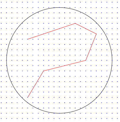
Figure 4: An example of a lattice $\Gamma_{\delta}$ in $\mathbb{R}^{2}$ with $\delta=1$ (spacing between blue points) and $B(0,10)$ (black circle). The red polygonal line is composed with vertices in $\mathcal{Q}_{\delta}=B(0,10)\cap\Gamma_{\delta}$.

Our goal is to learn a time-dependent polygonal line which passes through the "middle" of data and gives a summary of all available observations $x_{1},\dots,x_{t-1}$ (denoted by $(x_{s})_{1:(t-1)}$ hereafter) before time $t$. Our output at time $t$ is a polygonal line $\hat{\mathbf{f}}_{t}\in\mathcal{F}_{p}$ depending on past information $(x_{s})_{1:(t-1)}$ and past predictions $(\hat{\mathbf{f}}_{s})_{1:(t-1)}$. When $x_{t}$ is revealed, the instantaneous loss at time $t$ is computed as

$$\Delta\left(\hat{\mathbf{f}}_{t},x_{t}\right)=\inf_{s\in I}\ \|\hat{\mathbf{f}}_{t}(s)-x_{t}\|^{2}_{2}.$$ (2)

In what follows, we investigate regret bounds for the cumulative loss based on (2). Given a measurable space $\Theta$ (embedded with its Borel $\sigma$-algebra), we let $\mathcal{P}(\Theta)$ denote the set of probability distributions on $\Theta$, and for some reference measure $\pi$, we let $\mathcal{P}_{\pi}(\Theta)$ be the set of probability distributions absolutely continuous with respect to $\pi$.

For any $k\in\llbracket 1,p\rrbracket$, let $\pi_{k}$ denote a probability distribution on $\mathcal{F}_{k,L}$. We define the prior $\pi$ on $\mathcal{F}_{p}=\cup_{k=1}^{p}\mathcal{F}_{k,L}$ as

$$\pi(\mathbf{f})=\sum_{k\in\llbracket 1,p\rrbracket}w_{k}\pi_{k}(\mathbf{f})\mathbbm{1}_{\left\{\mathbf{f}\in\mathcal{F}_{k,L}\right\}},\quad\mathbf{f}\in\mathcal{F}_{p},$$

where $w_{1},\dots,w_{p}\geq 0$ and $\sum_{k\in\llbracket 1,p\rrbracket}w_{k}=1$.

We adopt a quasi-Bayesian-flavored procedure: consider the Gibbs quasi-posterior (note that this is not a proper posterior in all generality, hence the term "quasi")

$$\hat{\rho}_{t}(\cdot)\propto\exp(-\lambda S_{t}(\cdot))\pi(\cdot),$$

where

$$S_{t}(\mathbf{f})=S_{t-1}(\mathbf{f})+\Delta(\mathbf{f},x_{t})+\frac{\lambda}{2}\big{(}\Delta(\mathbf{f},x_{t})-\Delta(\hat{\mathbf{f}}_{t},x_{t})\big{)}^{2},$$

as advocated by Audibert (2009) and Li et al. (2018) who then consider realisations from this quasi-posterior. In the present paper, we will rather focus on a quantity linked to the mode of this quasi-posterior. Indeed, the mode of the quasi-posterior $\hat{\rho}_{t+1}$ is

$$\arg\min_{\mathbf{f}\in\mathcal{F}_{p}}\Bigg{\{}\underbrace{\sum_{s=1}^{t}\Delta(\mathbf{f},x_{s})}_{(i)}+\underbrace{\frac{\lambda}{2}\sum_{s=1}^{t}\big{(}\Delta(\mathbf{f},x_{t})-\Delta(\hat{\mathbf{f}}_{t},x_{t})\big{)}^{2}}_{(ii)}+\underbrace{\frac{\ln\pi(\mathbf{f})}{\lambda}}_{(iii)}\Bigg{\}},$$

where (i) is a cumulative loss term, (ii) is a term controlling the variance of the prediction $\mathbf{f}$ to past predictions $\hat{\mathbf{f}}_{s},s\leq t$, and (iii) can be regarded as a penalty function on the complexity of $\mathbf{f}$ if $\pi$ is well chosen. This mode hence has a similar flavor to follow the best expert or follow the perturbed leader in the setting of prediction with experts (see Hutter and Poland, 2005 and Cesa-Bianchi and Lugosi, 2006, Chapters 3 and 4) if we consider each $\mathbf{f}\in\mathcal{F}_{p}$ as an expert which always delivers constant advice. These remarks yield Algorithm 1.

Algorithm 1 Sequentially learning principal curves

1:Input parameters: $p>0,\eta>0,\pi(z)=\mathrm{e}^{-z}\mathbbm{1}_{\{z>0\}}$ and penalty function $h:\mathcal{F}_{p}\to\mathbb{R}^{+}$

2:Initialization: For each $\mathbf{f}\in\mathcal{F}_{p}$, draw $z_{\mathbf{f}}\sim\pi$ and $\Delta_{\mathbf{f},0}=\frac{1}{\eta}(h(\mathbf{f})-z_{\mathbf{f}})$

3:For $t=1,\dots,T$

4:      Get the data $x_{t}$

5:      Obtain

$$\hat{\mathbf{f}}_{t}=\underset{\mathbf{f}\in\mathcal{F}_{p}}{\arg\inf}\left\{\sum_{s=0}^{t-1}\Delta_{\mathbf{f},s}\right\},$$

      where $\Delta_{\mathbf{f},s}=\Delta(\mathbf{f},x_{s})$, $s\geq 1$.

6:End for

3 Regret bounds for sequential learning of principal curves

We now present our main theoretical results.

Theorem 1.

For any sequence $(x_{t})_{1:T}\in B(\text{0},\sqrt{d}R)$, $R\geq 0$ and any penalty function $h:\mathcal{F}_{p}\to\mathbb{R}^{+}$, let $\pi(z)=\mathrm{e}^{-z}\mathbbm{1}_{\{z>0\}}$. Let $0<\eta\leq\frac{1}{d(2R+\delta)^{2}}$, then the procedure described in Algorithm 1 satisfies

$$\sum_{t=1}^{T}\mathbb{E}_{\pi}\left[\Delta(\hat{\mathbf{f}}_{t},x_{t})\right]\leq\left(1+c_{0}(\mathrm{e}-1)\eta\right)S_{T,h,\eta}+\frac{1}{\eta}\left(1+\ln\sum_{\mathbf{f}\in\mathcal{F}_{p}}\mathrm{e}^{-h(\mathbf{f})}\right),$$

where $c_{0}=d(2R+\delta)^{2}$ and

$$S_{T,h,\eta}=\inf_{k\in\llbracket 1,p\rrbracket}\left\{\inf_{\begin{subarray}{c}\mathbf{f}\in\mathcal{F}_{p}\\ \mathcal{K}(\mathbf{f})=k\end{subarray}}\left\{\sum_{t=1}^{T}\Delta(\mathbf{f},x_{t})+\frac{h(\mathbf{f})}{\eta}\right\}\right\}.$$

The expectation of the cumulative loss of polygonal lines $\hat{\mathbf{f}}_{1},\dots,\hat{\mathbf{f}}_{T}$ is upper-bounded by the smallest penalised cumulative loss over all $k\in\{1,\dots,p\}$ up to a multiplicative term $(1+c_{0}(\mathrm{e}-1)\eta)$ which can be made arbitrarily close to 1 by choosing a small enough $\eta$. However, this will lead to both a large $h(\mathbf{f})/\eta$ in $S_{T,h,\eta}$ and a large $\frac{1}{\eta}(1+\ln\sum_{\mathbf{f}\in\mathcal{F}_{p}}\mathrm{e}^{-h(\mathbf{f})})$. In addition, another important issue is the choice of the penalty function $h$. For each $\mathbf{f}\in\mathcal{F}_{p}$, $h(\mathbf{f})$ should be large enough to ensure a small $\sum_{\mathbf{f}\in\mathcal{F}_{p}}\mathrm{e}^{-h(\mathbf{f})}$ while not too large to avoid overpenalization and a larger value for $S_{T,h,\eta}$. We therefore set

$$h(\mathbf{f})\geq\ln(p\mathrm{e})+\ln\bigg{|}\{\mathbf{f}\in\mathcal{F}_{p},\mathcal{K}(\mathbf{f})=k\}\bigg{|}$$ (3)

for each $\mathbf{f}$ with $k$ segments (where $|M|$ denotes the cardinality of a set $M$) since it leads to

$$\sum_{\mathbf{f}\in\mathcal{F}_{p}}\mathrm{e}^{-h(\mathbf{f})})=\sum_{k\in\llbracket 1,p\rrbracket}\sum_{\begin{subarray}{c}\mathbf{f}\in\mathcal{F}_{p}\\ \mathcal{K}(\mathbf{f})=k\end{subarray}}\mathrm{e}^{-h(\mathbf{f})}\leq\sum_{k\in\llbracket 1,p\rrbracket}\frac{1}{p\mathrm{e}}\leq\frac{1}{\mathrm{e}}.$$

The penalty function $h(\mathbf{f})=c_{1}\mathcal{K}(\mathbf{f})+c_{2}L+c_{3}$ satisfies (3), where $c_{1},c_{2},c_{3}$ are constants depending on $R$, $d$, $\delta$, $p$ (this is proven in Lemma 3, in Section 6). We therefore obtain the following corollary.

Corollary 1.

Under the assumptions of Theorem 1, let

$$\eta=\\ \min\left\{\frac{1}{d(2R+\delta)^{2}},\sqrt{\frac{c_{1}p+c_{2}L+c_{3}}{c_{0}(\mathrm{e}-1)\inf_{\mathbf{f}\in\mathcal{F}_{p}}\sum_{t=1}^{T}\Delta(\mathbf{f},x_{t})}}\right\}.$$

Then

$$\sum_{t=1}^{T}\mathbb{E}\left[\Delta(\hat{\mathbf{f}}_{t},x_{t})\right]\leq\inf_{k\in\llbracket 1,p\rrbracket}\left\{\inf_{\begin{subarray}{c}\mathbf{f}\in\mathcal{F}_{p}\\ \mathcal{K}(\mathbf{f})=k\end{subarray}}\left\{\sum_{t=1}^{T}\Delta(\mathbf{f},x_{t})+\sqrt{c_{0}(\mathrm{e}-1)r_{T,k,L}}\right\}\right\}\\ +\sqrt{c_{0}(\mathrm{e}-1)r_{T,p,L}}+c_{0}(\mathrm{e}-1)(c_{1}p+c_{2}L+c_{3}),$$

where $r_{T,k,L}=\inf_{\mathbf{f}\in\mathcal{F}_{p}}\sum_{t=1}^{T}\Delta(\mathbf{f},x_{t})(c_{1}k+c_{2}L+c_{3})$.

Proof.

Note that

$$\sum_{t=1}^{T}\mathbb{E}\left[\Delta(\hat{\mathbf{f}}_{t},x_{t})\right]\leq S_{T,h,\eta}+\eta c_{0}(\mathrm{e}-1)\inf_{\mathbf{f}\in\mathcal{F}_{p}}\sum_{t=1}^{T}\Delta(\mathbf{f},x_{t})+c_{0}(\mathrm{e}-1)(c_{0}p+c_{2}L+c_{3}),$$

and we conclude by setting

$$\eta=\sqrt{\frac{c_{1}p+c_{2}L+c_{3}}{c_{0}(\mathrm{e}-1)\inf_{\mathbf{f}\in\mathcal{F}_{p}}\sum_{t=1}^{T}\Delta(\mathbf{f},x_{t})}}.$$

∎

Sadly, Corollary 1 is not of much practical use since the optimal value for $\eta$ depends on $\inf_{\mathbf{f}\in\mathcal{F}_{p}}\sum_{t=1}^{T}\Delta(\mathbf{f},x_{t})$ which is obviously unknown, even more so at time $t=0$. We therefore provide an adaptive refinement of Algorithm 1 in the following Algorithm 2.

Algorithm 2 Sequentially and adaptively learning principal curves

1:Input parameters: $p>0$, $L>0$, $\pi$, $h$ and $\eta_{0}=\frac{\sqrt{c_{1}p+c_{2}L+c_{3}}}{c_{0}\sqrt{\mathrm{e}-1}}$

2:Initialization: For each $\mathbf{f}\in\mathcal{F}_{p}$, draw $z_{\mathbf{f}}\sim\pi$, $\Delta_{\mathbf{f},0}=\frac{1}{\eta_{0}}(h(\mathbf{f})-z_{\mathbf{f}})$ and $\hat{\mathbf{f}}_{0}=\underset{\mathbf{f}\in\mathcal{F}_{p}}{\mathrm{\arg\inf}}\ \Delta_{\mathbf{f},0}$

3:For $t=1,\dots,T$

4:      Compute $\eta_{t}=\frac{\sqrt{c_{1}p+c_{2}L+c_{3}}}{c_{0}\sqrt{(\mathrm{e}-1)t}}$

5:      Get data $x_{t}$ and compute $\Delta_{\mathbf{f},t}=\Delta(\mathbf{f},x_{t})+\left(\frac{1}{\eta_{t}}-\frac{1}{\eta_{t-1}}\right)\left(h(\mathbf{f})-z_{\mathbf{f}}\right)$

6:      Obtain

$$\hat{\mathbf{f}}_{t}=\underset{\mathbf{f}\in\mathcal{F}_{p}}{\mathrm{\arg\inf}}\ \left\{\sum_{s=0}^{t-1}\Delta_{\mathbf{f},s}\right\}.$$ (4)

7:End for

Theorem 2.

For any sequence $(x_{t})_{1:T}\in B(\text{0},\sqrt{d}R),R\geq 0$, let $h(\mathbf{f})=c_{1}\mathcal{K}(\mathbf{f})+c_{2}L+c_{3}$ where $c_{1}$, $c_{2}$, $c_{3}$ are constants depending on $R,d,\delta,\ln p$. Let $\pi(z)=\mathrm{e}^{-z}\mathbbm{1}_{\{z>0\}}$ and

$$\eta_{0}=\frac{\sqrt{c_{1}p+c_{2}L+c_{3}}}{c_{0}\sqrt{\mathrm{e}-1}},\quad\eta_{t}=\frac{\sqrt{c_{1}p+c_{2}L+c_{3}}}{c_{0}\sqrt{(\mathrm{e}-1)t}},$$

where $t\geq 1$ and $c_{0}=d(2R+\delta)^{2}$. Then the procedure described in Algorithm 2 satisfies

$$\sum_{t=1}^{T}\mathbb{E}\left[\Delta(\hat{\mathbf{f}}_{t},x_{t})\right]\leq\inf_{k\in\llbracket 1,p\rrbracket}\Bigg{\{}\inf_{\begin{subarray}{c}\mathbf{f}\in\mathcal{F}_{p}\\ \mathcal{K}(\mathbf{f})=k\end{subarray}}\bigg{\{}\sum_{t=1}^{T}\Delta(\mathbf{f},x_{t})+c_{0}\sqrt{(\mathrm{e}-1)T(c_{1}k+c_{2}L+c_{3})}\bigg{\}}\Bigg{\}}\\ +2c_{0}\sqrt{(\mathrm{e}-1)T(c_{1}p+c_{2}L+c_{3})}.$$

The message of this regret bound is that the expected cumulative loss of polygonal lines $\hat{\mathbf{f}}_{1},\dots,\hat{\mathbf{f}}_{T}$ is upper-bounded by the minimal cumulative loss over all $k\in\{1,\dots,p\}$, up to an additive term which is sublinear in $T$. The actual magnitude of this remainder term is $\sqrt{kT}$. When $L$ is fixed, the number $k$ of segments is a measure of complexity of the retained polygonal line. This bound therefore yields the same magnitude than (1) which is the most refined bound in the literature so far (Biau and Fischer, 2012, where the optimal values for $k$ and $L$ are obtained in a model selection fashion).

4 Implementation

The argument of the infimum in Algorithm 2 is taken over $\mathcal{F}_{p}=\cup_{k=1}^{p}\mathcal{F}_{k,L}$ which has a cardinality of order $\left|\mathcal{Q}_{\delta}\right|^{p}$, making any greedy search largely time-consuming. We instead turn to the following strategy: given a polygonal line $\hat{\mathbf{f}}_{t}\in\mathcal{F}_{k_{t},L}$ with $k_{t}$ segments, we consider, with a certain proportion, the availability of $\hat{\mathbf{f}}_{t+1}$ within a neighbourhood $\mathcal{U}(\hat{\mathbf{f}}_{t})$ (see the formal definition below) of $\hat{\mathbf{f}}_{t}$. This consideration is well suited for the principal curves setting since if observation $x_{t}$ is close to $\hat{\mathbf{f}}_{t}$, one can expect that the polygonal line which well fits observations $x_{s},s=1,\dots,t$ lies in a neighbourhood of $\hat{\mathbf{f}}_{t}$. In addition, if each polygonal line $\mathbf{f}$ is regarded as an action, we no longer assume that all actions are available at all times, and allow the set of available actions to vary at each time. This is a model known as "sleeping experts (or actions)" in prior work (Auer et al., 2003; Kleinberg et al., 2008). In this setting, defining the regret with respect to the best action in the whole set of actions in hindsight remains difficult since that action might sometimes be unavailable. Hence it is natural to define the regret with respect to the best ranking of all actions in the hindsight according to their losses or rewards, and at each round one chooses among the available actions by selecting the one which ranks the highest. Kleinberg et al. (2008) introduced this notion of regret and studied both the full-information (best action) and partial-information (multi-armed bandit) settings with stochastic and adversarial rewards and adversarial action availability. They pointed out that the EXP4 algorithm (Auer et al., 2003) attains the optimal regret in adversarial rewards case but has a runtime exponential in the number of all actions. Kanade et al. (2009) considered full and partial information with stochastic action availability and proposed an algorithm that runs in polynomial time. In what follows, we materialize our implementation by resorting to ”sleeping experts” i.e., a special set of available actions that adapts to the setting of principal curves.

Let $\sigma$ denote an ordering of $|\mathcal{F}_{p}|$ actions, and $\mathcal{A}_{t}$ a subset of the available actions at round $t$. We let $\sigma(\mathcal{A}_{t})$ denote the highest ranked action in $\mathcal{A}_{t}$. In addition, for any action $\mathbf{f}\in\mathcal{F}_{p}$ we define the reward $r_{\mathbf{f},t}$ of $\mathbf{f}$ at round $t,t\geq 0$ by

$$r_{\mathbf{f},t}=c_{0}-\Delta(\mathbf{f},x_{t}).$$

It is clear that $r_{\mathbf{f},t}\in(0,c_{0})$. The convention from losses to gains is done in order to facilitate the subsequent performance analysis. The reward of an ordering $\sigma$ is the cumulative reward of the selected action at each time

$$\sum_{t=1}^{T}r_{\sigma(\mathcal{A}_{t}),t},$$

and the reward of the best ordering is $\max_{\sigma}\sum_{t=0}^{T}r_{\sigma(\mathcal{A}_{t}),t}$ (respectively, $\mathbb{E}\left[\max_{\sigma}\sum_{t=1}^{T}r_{\sigma(\mathcal{A}_{t}),t}\right]$ when $\mathcal{A}_{t}$ is stochastic).

Our procedure starts with a partition step which aims at identifying the "relevant" neighbourhood of an observation $x\in\mathbb{R}^{d}$ with respect to a given polygonal line, and then proceeds with the definition of the neighbourhood of an action $\mathbf{f}$. We then provide the full implementation and prove a regret bound.

Partition For any polygonal line $\mathbf{f}$ with $k$ segments, we denote by $\overset{\rightharpoonup}{\mathbf{V}}=\left(v_{1},\dots,v_{k+1}\right)$ its vertices and by $s_{i},i=1,\dots,k$ the line segments connecting $v_{i}$ and $v_{i+1}$. In the sequel, we use $\mathbf{f}(\overset{\rightharpoonup}{\mathbf{V}})$ to represent the polygonal line formed by connecting consecutive vertices in $\overset{\rightharpoonup}{\mathbf{V}}$ if no confusion arises. Let $V_{i},i=1,\dots,k+1$ and $S_{i},i=1,\dots,k$ be the Voronoi partitions of $\mathbb{R}^{d}$ with respect to $\mathbf{f}$, i.e., regions consisting of all points closer to vertex $v_{i}$ or segment $s_{i}$. Figure 5 shows an example of Voronoi partition with respect to $\mathbf{f}$ with 3 segments.

Neighbourhood For any $x\in\mathbb{R}^{d}$, we define the neighbourhood $\mathcal{N}(x)$ with respect to $\mathbf{f}$ as the union of all Voronoi partitions whose closure intersects with two vertices connecting the projection $\mathbf{f}(s_{\mathbf{f}}(x))$ of $x$ to $\mathbf{f}$. For example, for the point $x$ in Figure 5, its neighbourhood $\mathcal{N}(x)$ is the union of $S_{2},V_{3},S_{3}$ and $V_{4}$. In addition, let $\mathcal{N}_{t}(x)=\left\{x_{s}\in\mathcal{N}\left(x\right),s=1,\dots,t.\right\}$ be the set of observations $x_{1:t}$ belonging to $\mathcal{N}\left(x\right)$ and $\bar{\mathcal{N}}_{t}(x)$ be its average. Let $\mathcal{D}(M)=\sup_{x,y\in M}||x-y||_{2}$ denote the diameter of set $M\subset\mathbb{R}^{d}$. We finally define the local grid $\mathcal{Q}_{\delta,t}(x)$ of $x\in\mathbb{R}^{d}$ at time $t$ as

$$\mathcal{Q}_{\delta,t}(x)=B\left(\bar{\mathcal{N}}_{t}(x),\mathcal{D}\left(\mathcal{N}_{t}(x\right)\right)\cap\mathcal{Q}_{\delta}.$$

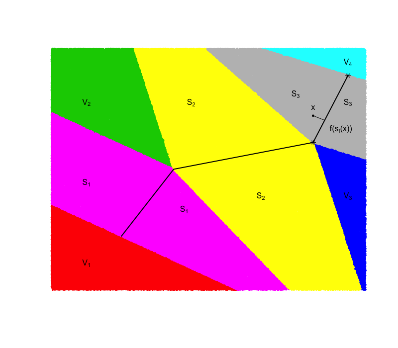
Figure 5: An example of a Voronoi partition.

We can finally proceed to the definition of the neighbourhood $\mathcal{U}(\hat{\mathbf{f}}_{t})$ of $\hat{\mathbf{f}}_{t}$. Assume $\hat{\mathbf{f}}_{t}$ has $k_{t}+1$ vertices $\overset{\rightharpoonup}{\mathbf{V}}=(\underbrace{v_{1:i_{t}-1}}_{(i)},\underbrace{v_{i_{t}:j_{t}-1}}_{(ii)},\underbrace{v_{j_{t}:k_{t}+1}}_{(iii)})$, where vertices of $(ii)$ belong to $\mathcal{Q}_{\delta,t}(x_{t})$ while those of $(i)$ and $(iii)$ do not. The neighbourhood $\mathcal{U}(\hat{\mathbf{f}}_{t})$ consists of $\mathbf{f}$ sharing vertices $(i),(iii)$ with $\hat{\mathbf{f}}_{t}$, but can be equipped with different vertices $(ii)$ in $\mathcal{Q}_{\delta,t}(x_{t})$, i.e.,

$$\mathcal{U}(\hat{\mathbf{f}}_{t})=\left\{\mathbf{f}(\overset{\rightharpoonup}{\mathbf{V}}),\quad\overset{\rightharpoonup}{\mathbf{V}}=\left(v_{1:i_{t}-1},v_{1:m},v_{j_{t}:k_{t}+1}\right)\right\},$$

where $v_{1:m}\in\mathcal{Q}_{\delta,t}(x_{t})$ and $m$ is given by

$$m=\begin{cases}j_{t}-i_{t}-1&\mbox{reduce segments by 1 unit},\\ j_{t}-i_{t}&\mbox{same number of segments},\\ j_{t}-i_{t}+1&\mbox{increase segments by 1 unit}.\end{cases}$$

Algorithm 3 A locally greedy algorithm to sequentially learn principal curves

1:Input parameters: $p>0$, $R>0$, $L>0$, $\epsilon>0$, $\alpha>0$, $1>\beta>0$ and any penalty function $h$

2:Initialization: Given $(x_{t})_{1:t_{0}}$, obtain $\hat{\mathbf{f}}_{1}$ as the first principal component

3:For $t=2,\dots,T$

4:      Draw $I_{t}\sim Bernoulli(\epsilon)$ and $z_{\mathbf{f}}\sim\pi$.

5:      Let

$$\hat{\sigma}_{t}=\text{sort}\left(\mathbf{f},\quad\sum_{s=1}^{t-1}\hat{r}_{\mathbf{f},s}-\frac{1}{\eta_{t-1}}h(\mathbf{f})+\frac{1}{\eta_{t-1}}z_{\mathbf{f}}\right),$$

i.e., sorting all $\mathbf{f}\in\mathcal{F}_{p}$ in descending order according to their perturbed cumulative reward till $t-1$.

6:      If $I_{t}=1$, set $\mathcal{A}_{t}=\mathcal{F}_{p}$ and $\hat{\mathbf{f}}_{t}=\hat{\sigma}^{t}(\mathcal{A}_{t})$ and observe $r_{\hat{\mathbf{f}}_{t},t}$

7:               

$$\hat{r}_{\mathbf{f},t}=r_{\mathbf{f},t}\quad\text{for}\quad\mathbf{f}\in\mathcal{F}_{p}.$$

8:      If $I_{t}=0$, set $\mathcal{A}_{t}=\mathcal{U}(\hat{\mathbf{f}}_{t-1})$, $\hat{\mathbf{f}}_{t}=\hat{\sigma}^{t}(\mathcal{A}_{t})$ and observe $r_{\hat{\mathbf{f}}_{t},t}$

9:               

$$\hat{r}_{\mathbf{f},t}=\begin{cases}\frac{r_{\mathbf{f},t}}{\mathbb{P}\left(\hat{\mathbf{f}}_{t}=\mathbf{f}|\mathcal{H}_{t}\right)}&\mbox{if \, $\mathbf{f}\in\mathcal{U}(\hat{\mathbf{f}}_{t-1})\cap cond(t)$}\text{ and }\hat{\mathbf{f}}_{t}=\mathbf{f},\\ \alpha&\mbox{\text{otherwise}},\end{cases}$$

where $\mathcal{H}_{t}$ denotes all the randomness before time $t$ and $\mathit{cond}(t)=\left\{\mathbf{f}\in\mathcal{F}_{p}:\mathbb{P}\left(\hat{\mathbf{f}}_{t}=\mathbf{f}|\mathcal{H}_{t}\right)>\beta\right\}$. In particular, when $t=1$, we set $\hat{r}_{\mathbf{f},1}=r_{\mathbf{f},1}$ for all $\mathbf{f}\in\mathcal{F}_{p}$, $\mathcal{U}\left(\hat{\mathbf{f}}_{0}\right)=\emptyset$ and $\hat{r}_{\hat{\sigma}^{1}\left(\mathcal{U}\left(\hat{\mathbf{f}}_{0}\right)\right),1}\equiv 0$.

10:End for

In Algorithm 3, we initiate the principal curve $\hat{\mathbf{f}}_{1}$ as the first component line segment whose vertices are the two farthest projections of data $x_{1:t_{0}}$ ($t_{0}$ can be set to 2 or 3 in practice) on the first component line. The reward of $\mathbf{f}$ at round $t$ in this setting is therefore $r_{\mathbf{f},t}=c_{0}-\Delta(\mathbf{f},x_{t_{0}+t})$. Algorithm 3 has an exploration phase (when $I_{t}=1$) and an exploitation phase ($I_{t}=0$). In the exploration phase, it is allowed to observe rewards of all actions and to choose an optimal perturbed action from the set $\mathcal{F}_{p}$ of all actions. In the exploitation phase, only rewards of a part of actions can be accessed and rewards of others are estimated by a constant, and we update our action from the neighbourhood $\mathcal{U}\left(\hat{\mathbf{f}}_{t-1}\right)$ of the previous action $\hat{\mathbf{f}}_{t-1}$. This local update (or search) greatly reduces computation complexity since $|\mathcal{U}(\hat{\mathbf{f}}_{t-1})|\ll\left|\mathcal{F}_{p}\right|$ when $p$ is large. In addition, this local search will be enough to account for the case when $x_{t}$ locates in $\mathcal{U}\left(\hat{\mathbf{f}}_{t-1}\right)$. The parameter $\beta$ needs to be carefully calibrated since it should not be too large to ensure that the condition $cond(t)$ is non-empty, otherwise all rewards are estimated by the same constant and thus lead to the same descending ordering of tuples for both $\left(\sum_{s=1}^{t-1}\hat{r}_{\mathbf{f},s},\mathbf{f}\in\mathcal{F}_{p}\right)$ and $\left(\sum_{s=1}^{t}\hat{r}_{\mathbf{f},s},\mathbf{f}\in\mathcal{F}_{p}\right)$. Therefore, we may face the risk of having $\hat{\mathbf{f}}_{t+1}$ in the neighbourhood of $\hat{\mathbf{f}}_{t}$ even if we are in the exploration phase at time $t+1$. Conversely, very small $\beta$ could result in large bias for the estimation $\frac{r_{\mathbf{f},t}}{\mathbb{P}\left(\hat{\mathbf{f}}_{t}=\mathbf{f}|\mathcal{H}_{t}\right)}$ of $r_{\mathbf{f},t}$. Note that the exploitation phase is close yet different to the label efficient prediction (Cesa-Bianchi et al., 2005, Remark 1.1) since we allow an action at time $t$ to be different from the previous one. Neu and Bartók (2013) have proposed the Geometric Resampling method to estimate the conditional probability $\mathbb{P}\left(\hat{\mathbf{f}}_{t}=\mathbf{f}|\mathcal{H}_{t}\right)$ since this quantity often does not have an explicit form. However, due to the simple exponential distribution of $z_{\mathbf{f}}$ chosen in our case, an explicit form of $\mathbb{P}\left(\hat{\mathbf{f}}_{t}=\mathbf{f}|\mathcal{H}_{t}\right)$ is straightforward.

Theorem 3.

Assume that $p>6$, $T\geq 2|\mathcal{F}_{p}|^{2}$ and let $\beta=\left|\mathcal{F}_{p}\right|^{-\frac{1}{2}}T^{-\frac{1}{4}}$, $\alpha=\frac{c_{0}}{\beta}$, $\hat{c}_{0}=\frac{2c_{0}}{\beta}$, $\epsilon=1-\left|\mathcal{F}_{p}\right|^{\frac{1}{2}-\frac{3}{p}}T^{-\frac{1}{4}}$ and

$$\eta_{1}=\eta_{2}=\dots=\eta_{T}=\frac{\sqrt{c_{1}p+c_{2}L+c_{3}}}{\sqrt{T(e-1)}\hat{c}_{0}}.$$

Then the procedure described in Algorithm 3 satisfies the regret bound

$$\sum_{t=1}^{T}\mathbb{E}\left[\Delta\left(\hat{\mathbf{f}}_{t},x_{t}\right)\right]\leq\inf_{\mathbf{f}\in\mathcal{F}_{p}}\mathbb{E}\left[\sum_{t=1}^{T}\Delta\left(\mathbf{f},t\right)\right]+\mathcal{O}(T^{\frac{3}{4}}).$$

The proof of Theorem 3 is presented in Section 6. The regret is upper bounded by a term of order $\left(\left|\mathcal{F}_{p}\right|^{\frac{1}{2}}T^{\frac{3}{4}}\right)$, sublinear in $T$. The term $(1-\epsilon)c_{0}T=c_{0}\left|\mathcal{F}_{p}\right|^{\frac{1}{2}}T^{\frac{3}{4}}$ is the price to pay for the local search (with a proportion $1-\epsilon$) of polygonal line $\hat{\mathbf{f}}_{t}$ in the neighbourhood of the previous $\hat{\mathbf{f}}_{t-1}$. If $\epsilon=1$, we would have that $\hat{c}_{0}=c_{0}$ and the last two terms in the first inequality of Theorem 3 would vanish, hence the upper bound reduces to Theorem 2. In addition, our algorithm achieves an order that is smaller (from the perspective of both the number $\left|\mathcal{F}_{p}\right|$ of all actions and the total rounds $T$) than Kanade et al. (2009) since at each time, the availability of actions for our algorithm can be either the whole action set or a neighbourhood of the previous action while Kanade et al. (2009) consider at each time only partial and independent stochastic available set of actions generated from a predefined distribution.

5 Numerical experiments

We illustrate the performance of Algorithm 3 on synthetic and real-life data. Our implementation (hereafter denoted by slpc – Sequential Learning of Principal Curves) is conducted with the R language and thus our most natural competitor is the R package princurve (which is the algorithm from Hastie and Stuetzle, 1989). We let $p=20$, $R=\max_{t=1,\dots,T}||x||_{2}/\sqrt{d}$, $L=0.01p\sqrt{d}R$. The spacing $\delta$ of the lattice is ajusted with respect to data scale.

Synthetic data We generate a data set $\left\{x_{t}\in\mathbb{R}^{2},t=1,\dots,100\right\}$ uniformly along the curve $y=0.05\times(x-5)^{3}$, $x\in[0,10]$. Table 1 shows the regret for the ground truth (sum of squared distances of all points to the true curve), princurve (sum of squared distances between observation $t+1$ and fitted princurve trained on all past $t$ observations) and slpc ($\sum_{t=0}^{T-1}\Delta(\hat{\mathbf{f}}_{t+1},x_{t+1})$). slpc greatly outperforms princurve on this example, as illustrated by Figure 8 and Figure 9.

ground truth	princurve	slpc
0.945 (0)	25.387 (0)	9.893 (0.246)

Table 1: Regret (cumulative loss) on synthetic data (average over 10 trials, with standard deviation in brackets). princurve is deterministic, hence the zero standard deviation.

Synthetic data in high dimension We also apply our algorithm on a data set $\left\{x_{t}\in\mathbb{R}^{6},t=1,2,\dots,200\right\}$ in higher dimension. It is generated uniformly along a parametric curve whose coordinates are

$$\begin{pmatrix}0.5t\cos(t)\\ 0.5t\sin(t)\\ 0.5t\\ -t\\ \sqrt{t}\\ 2\ln(t+1)\end{pmatrix}$$

where $t$ takes 100 equidistant values in $[0,2\pi]$. To the best of our knowledge, Hastie and Stuetzle (1989), Kégl (1999) and Biau and Fischer (2012) only tested their algorithm on 2-dimensional data. This example aims at illustrating that our algorithm also works on higher dimensional data. Table 2 shows the regret for the ground truth, princurve and slpc.

ground truth	princurve	slpc
3.290 (0)	14.204 (0)	6.797 (0.409)

Table 2: Regret (cumulative loss) on synthetic data in higher dimension (average over 10 trials, with standard deviation in brackets). princurve is deterministic.

In addition, Figure 6 shows the behaviour of slpc (green) on each dimension.

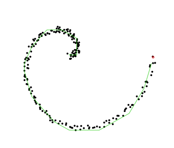
(a) slpc, $t=199$, 1st and 2nd coordinates

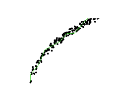
(b) slpc, $t=199$, 3th and 5th coordinates

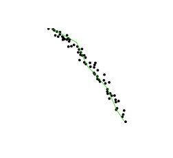
(c) slpc, $t=199$, 4th and 6th coordinates

Figure 6: slpc (green line) on synthetic data in higher dimension from different perspectives. Black dots represent recordings $x_{1:99}$, the red dot is the new recording $x_{200}$.

Seismic data Seismic data spanning long periods of time are essential for a thorough understanding of earthquakes. The “Centennial Earthquake Catalog” (Engdahl and Villaseñor, 2002) aims at providing a realistic picture of the seismicity distribution on Earth. It consists in a global catalog of locations and magnitudes of instrumentally recorded earthquakes from 1900 to 2008. We focus on a particularly representative seismic active zone (a lithospheric border close to Australia) whose longitude is between E$130^{\circ}$ to E$180^{\circ}$ and latitude between S$70^{\circ}$ to N$30^{\circ}$, with $T=218$ seismic recordings. As shown in Figure 7, slpc recovers nicely the tectonic plate boundary. Lastly, since no ground truth is available, we use the $R^{2}$ coefficient to assess the performance (residuals are replaced by the squared distance between data points and their projections onto the principal curve). The average over 10 trials is 0.990.

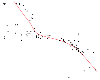
(a) princurve, $t=100$

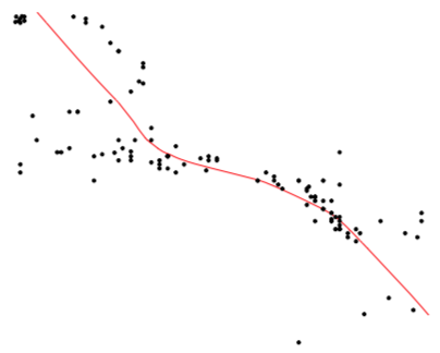
(b) princurve, $t=125$

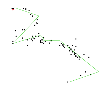
(c) slpc, $t=100$

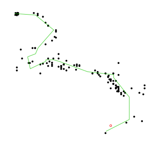
(d) slpc, $t=125$

Figure 7: Seismic data. Black dots represent seismic recordings $x_{1:t}$, red dot is the new recording $x_{t+1}$.

Back to the synthetic data setting

Figure 8 presents the predicted principal curve $\hat{\mathbf{f}}_{t+1}$ for both princurve (red) and slpc (green). The output of princurve yields a curve which does not pass in "the middle of data" but rather bends towards the curvature of the data cloud: slpc does not suffer from this behavior. To better illustrate the way slpc works between two epochs, Figure 9 focuses on the impact of collecting a new data point on the principal curve. We see that only a local vertex is impacted, whereas the rest of the principal curve remains unaltered. This cutdown in algorithmic complexity is one the key assets of slpc.

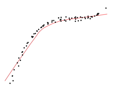
(a) $t=75$, princurve

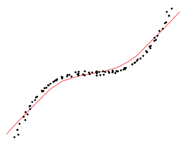
(b) $t=100$, princurve

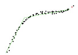
(c) $t=75$, slpc

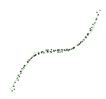
(d) $t=100$, slpc

Figure 8: Synthetic data - Black dots represent data $x_{1:t}$, red point is the new observation $x_{t+1}$. princurve (solid red) and slpc (solid green).

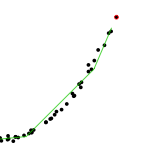
(a) At time $t=97$

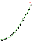
(b) And at time $t=98$

Figure 9: Synthetic data - Zooming in: how a new data point impacts only locally the principal curve.

Back to seismic data

Figure 10 is taken from the USGS website and gives the global earthquakes locations on the period 1900–1999. The seismic data (latitude, longitude, magnitude of earthquakes, etc.) used in the present paper may be downloaded from this website.

Daily commute data

The identification of segments of personal daily commuting trajectories can help taxi or bus companies to optimise their fleets and increase frequencies on segments with high commuting activity. Sequential principal curves appear to be an ideal tool to address this learning problem: we test our algorithm on trajectory data from the University of Illinois at Chicago . The data is obtained from the GPS reading systems carried by two of the lab members during their daily commute for 6 months in the Cook county and the Dupage county of Illinois. Figure 11 presents the learning curves yielded by princurve and slpc on geolocalization data for the first person, on May 30 in the data set. A particularly remarkable asset of slpc is that abrupt curvature in the data sequence is perfectly captured, whereas princurve does not enjoy the same flexibility. Again, we use the $R^{2}$ coefficient to assess the performance (where residuals are replaced by the squared distance between data points and their projections onto the principal curve). The average over 10 trials is 0.998.

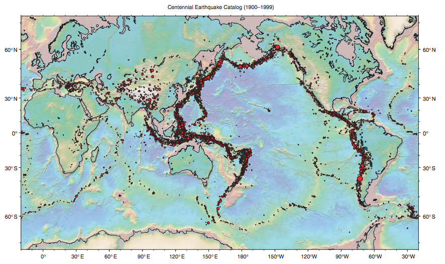
Figure 10: Seismic data from https://earthquake.usgs.gov/data/centennial/

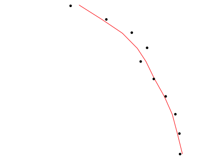
(a) $t=10$, princurve

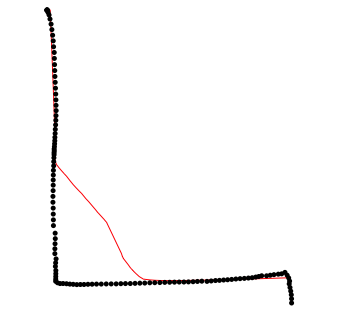
(b) $t=127$, princurve

(c) $t=10$, slpc

(d) $t=127$, slpc

Figure 11: Daily commute data - Black dots represent collected locations $x_{1:t}$, red point is the new observation $x_{t+1}$. princurve (solid red) and slpc (solid green).

6 Proofs

This section contains the proof of Theorem 2 (note that Theorem 1 is a straightforward consequence, with $\eta_{t}=\eta$, $t=0,\dots,T$) and the proof of Theorem 3 (which involves intermediary lemmas). Let us first define for each $t=0,\dots,T$ the following forecaster sequence $(\hat{\mathbf{f}}^{\star}_{t})_{t}$

$$\hat{\mathbf{f}}_{0}^{\star}=\underset{\mathbf{f}\in\mathcal{F}_{p}}{\arg\inf}\,\left\{\Delta_{\mathbf{f},0}\right\}=\underset{\mathbf{f}\in\mathcal{F}_{p}}{\arg\inf}\left\{\frac{1}{\eta_{0}}h(\mathbf{f})-\frac{1}{\eta_{0}}z_{\mathbf{f}}\right\},$$

$$\hat{\mathbf{f}}^{\star}_{t}=\underset{\mathbf{f}\in\mathcal{F}_{p}}{\arg\inf}\,\left\{\sum_{s=0}^{t}\Delta_{\mathbf{f},s}\right\}=\underset{\mathbf{f}\in\mathcal{F}_{p}}{\arg\inf}\left\{\sum_{s=1}^{t}\Delta(\mathbf{f},x_{s})+\frac{1}{\eta_{t-1}}h(\mathbf{f})-\frac{1}{\eta_{t-1}}z_{\mathbf{f}}\right\},\quad t\geq 1.$$

Note that $\hat{\mathbf{f}}^{\star}_{t}$ is an "illegal" forecaster since it peeks into the future. In addition, denote by

$$\mathbf{f}^{\star}=\underset{\mathbf{f}\in\mathcal{F}_{p}}{\arg\inf}\left\{\sum_{t=1}^{T}\Delta(\mathbf{f},x_{t})+\frac{1}{\eta_{T}}h(\mathbf{f})\right\}$$

the polygonal line in $\mathcal{F}_{p}$ which minimizes the cumulative loss in the first $T$ rounds plus a penalty term. $\mathbf{f}^{\star}$ is deterministic while $\hat{\mathbf{f}}^{\star}_{t}$ is a random quantity (since it depends on $z_{\mathbf{f}}$, $\mathbf{f}\in\mathcal{F}_{p}$ drawn from $\pi$). If several $\mathbf{f}$ attain the infimum, we choose $\mathbf{f}^{\star}_{T}$ as the one having the smallest complexity. We now enunciate the first (out of three) intermediary technical result.

Lemma 1.

For any sequence $x_{1},\dots,x_{T}$ in $B(\text{0},\sqrt{d}R)$,

$$\sum_{t=0}^{T}\Delta_{\hat{\mathbf{f}}_{t}^{\star},t}\leq\sum_{t=0}^{T}\Delta_{\hat{\mathbf{f}}_{T}^{\star},t},\qquad\pi\text{-almost surely}.$$ (5)

Proof.

Proof by induction on $T$. Clearly (5) holds for $T=0$. Assume that (5) holds for $T-1$:

$$\sum_{t=0}^{T-1}\Delta_{\hat{\mathbf{f}}_{t}^{\star},t}\leq\sum_{t=0}^{T-1}\Delta_{\hat{\mathbf{f}}_{T-1}^{\star},t}.$$

Adding $\Delta_{\hat{\mathbf{f}}_{T}^{\star},T}$ to both sides of the above inequality concludes the proof. ∎

By (5) and the definition of $\hat{\mathbf{f}}_{T}^{\star}$, for $k\geq 1$, we have $\pi$-almost surely that

$$\sum_{t=1}^{T}\Delta(\hat{\mathbf{f}}_{t}^{\star},x_{t}) \leq\sum_{t=1}^{T}\Delta(\hat{\mathbf{f}}_{T}^{\star},x_{t})+\frac{1}{\eta_{T}}h(\hat{\mathbf{f}}_{T}^{\star})-\frac{1}{\eta_{T}}Z_{\hat{\mathbf{f}}_{T}^{\star}}+\sum_{t=0}^{T}\left(\frac{1}{\eta_{t-1}}-\frac{1}{\eta_{t}}\right)\left(h(\hat{\mathbf{f}}_{t}^{\star})-Z_{\hat{\mathbf{f}}_{t}^{\star}}\right)$$

$$\leq\sum_{t=1}^{T}\Delta(\mathbf{f}^{\star},x_{t})+\frac{1}{\eta_{T}}h(\mathbf{f}^{\star})-\frac{1}{\eta_{T}}Z_{\mathbf{f}^{\star}}+\sum_{t=0}^{T}\left(\frac{1}{\eta_{t-1}}-\frac{1}{\eta_{t}}\right)\left(h(\hat{\mathbf{f}}_{t}^{\star})-Z_{\hat{\mathbf{f}}_{t}^{\star}}\right)$$

$$=\inf_{\mathbf{f}\in\mathcal{F}_{p}}\left\{\sum_{t=1}^{T}\Delta(\mathbf{f},x_{t})+\frac{1}{\eta_{T}}h(\mathbf{f})\right\}-\frac{1}{\eta_{T}}Z_{\mathbf{f}^{\star}}+\sum_{t=0}^{T}\left(\frac{1}{\eta_{t-1}}-\frac{1}{\eta_{t}}\right)\left(h(\hat{\mathbf{f}}_{t}^{\star})-Z_{\hat{\mathbf{f}}_{t}^{\star}}\right),$$

where $1/\eta_{-1}=0$ by convention. The second and third inequality is due to respectively the definition of $\hat{\mathbf{f}}_{T}^{\star}$ and $\mathbf{f}_{T}^{\star}$. Hence

$$\mathbb{E}\left[\sum_{t=1}^{T}\Delta\left(\hat{\mathbf{f}}_{t}^{\star},x_{t}\right)\right] \leq\inf_{\mathbf{f}\in\mathcal{F}_{p}}\left\{\sum_{t=1}^{T}\Delta(\mathbf{f},x_{t})+\frac{1}{\eta_{T}}h(\mathbf{f})\right\}-\frac{1}{\eta_{T}}\mathbb{E}[Z_{\mathbf{f}^{\star}_{T}}]+\sum_{t=0}^{T}\mathbb{E}\left[\left(\frac{1}{\eta_{t}}-\frac{1}{\eta_{t-1}}\right)\left(-h(\hat{\mathbf{f}}_{t}^{\star})+Z_{\hat{\mathbf{f}}_{t}^{\star}}\right)\right]$$

$$\leq\inf_{\mathbf{f}\in\mathcal{F}_{p}}\left\{\sum_{t=1}^{T}\Delta(\mathbf{f},x_{t})+\frac{1}{\eta_{T}}h(\mathbf{f})\right\}+\sum_{t=1}^{T}\left(\frac{1}{\eta_{t}}-\frac{1}{\eta_{t-1}}\right)\mathbb{E}\left[\sup_{\mathbf{f}\in\mathcal{F}_{p}}\left(-h(\mathbf{f})+Z_{\mathbf{f}}\right)\right]$$

$$=\inf_{\mathbf{f}\in\mathcal{F}_{p}}\left\{\sum_{t=1}^{T}\Delta(\mathbf{f},x_{t})+\frac{1}{\eta_{T}}h(\mathbf{f})\right\}+\frac{1}{\eta_{T}}\mathbb{E}\left[\sup_{\mathbf{f}\in\mathcal{F}_{p}}\left(-h(\mathbf{f})+Z_{\mathbf{f}}\right)\right],$$

where the second inequality is due to $\mathbb{E}[Z_{\mathbf{f}^{\star}_{T}}]=0$ and $\left(\frac{1}{\eta_{t}}-\frac{1}{\eta_{t-1}}\right)>0$ for $t=0,1,\dots,T$ since $\eta_{t}$ is decreasing in $t$ in Theorem 2. In addition, for $y\geq 0$, one has

$$\mathbb{P}\left(-h(\mathbf{f})+Z_{\mathbf{f}}>y\right)=\mathrm{e}^{-h(\mathbf{f})-y}.$$

Hence, for any $y\geq 0$

$$\mathbb{P}\left(\sup_{\mathbf{f}\in\mathcal{F}_{p}}\left(-h(\mathbf{f})+Z_{\mathbf{f}}\right)>y\right)\leq\sum_{\mathbf{f}\in\mathcal{F}_{p}}\mathbb{P}\left(Z_{\mathbf{f}}\geq h(\mathbf{f})+y\right)=\sum_{\mathbf{f}\in\mathcal{F}_{p}}\mathrm{e}^{-h(\mathbf{f})}\mathrm{e}^{-y}=u\mathrm{e}^{-y},$$

where $u=\sum_{\mathbf{f}\in\mathcal{F}_{p}}\mathrm{e}^{-h(\mathbf{f})}$. Therefore, we have

$$\mathbb{E}\left[\sup_{\mathbf{f}\in\mathcal{F}_{p}}\left(-h(\mathbf{f})+Z_{\mathbf{f}}\right)-\ln u\right] \leq\mathbb{E}\left[\max\left(0,\sup_{\mathbf{f}\in\mathcal{F}_{p}}\left(-h(\mathbf{f})+Z_{\mathbf{f}}-\ln u\right)\right)\right]$$

$$\leq\int_{0}^{\infty}\mathbb{P}\left(\max\left(0,\sup_{\mathbf{f}\in\mathcal{F}_{p}}\left(-h(\mathbf{f})+Z_{\mathbf{f}}-\ln u\right)\right)>y\right)\mathrm{d}y$$

$$\leq\int_{0}^{\infty}\mathbb{P}\left(\sup_{\mathbf{f}\in\mathcal{F}_{p}}\left(-h(\mathbf{f})+Z_{\mathbf{f}}\right)>y+\ln u\right)\mathrm{d}y$$

$$\leq\int_{0}^{\infty}u\mathrm{e}^{-(y+\ln u)}\mathrm{d}y=1.$$

We thus obtain

$$\mathbb{E}\left[\sum_{t=1}^{T}\Delta\left(\hat{\mathbf{f}}_{t}^{\star},x_{t}\right)\right]\leq\inf_{\mathbf{f}\in\mathcal{F}_{p}}\left\{\sum_{t=1}^{T}\Delta(\mathbf{f},x_{t})+\frac{1}{\eta_{T}}h(\mathbf{f})\right\}+\frac{1}{\eta_{T}}\left(1+\ln\sum_{\mathbf{f}\in\mathcal{F}_{p}}\mathrm{e}^{-h(\mathbf{f})}\right).$$ (6)

Next, we control the regret of Algorithm 2.

Lemma 2.

Assume that $z_{\mathbf{f}}$ is sampled from the symmetric exponential distribution in $\mathbb{R}$, i.e., $\pi(z)=\mathrm{e}^{-z}\mathbbm{1}_{\{z>0\}}$. Assume that $\sup_{t=1,\dots,T}\eta_{t-1}\leq\frac{1}{d(2R+\delta)^{2}}$, and define $c_{0}=d(2R+\delta)^{2}$. Then for any sequence $(x_{t})\in B(\text{0},\sqrt{d}R)$, $t=1,\dots,T$,

$$\sum_{t=1}^{T}\mathbb{E}\left[\Delta\left(\hat{\mathbf{f}}_{t},x_{t}\right)\right]\leq\sum_{t=1}^{T}\left(1+\eta_{t-1}c_{0}(\mathrm{e}-1)\right)\mathbb{E}\left[\Delta\left(\hat{\mathbf{f}}_{t}^{\star},x_{t}\right)\right].$$ (7)

Proof.

Let us denote by

$$F_{t}(Z_{\mathbf{f}})=\Delta\left(\hat{\mathbf{f}}_{t},x_{t}\right)=\Delta\left(\underset{\mathbf{f}\in\mathcal{F}}{\arg\inf}\left(\sum_{s=1}^{t-1}\Delta(\mathbf{f},x_{s})+\frac{1}{\eta_{t-1}}h(\mathbf{f})-\frac{1}{\eta_{t-1}}Z_{\mathbf{f}}\right),x_{t}\right)$$

the instantaneous loss suffered by the polygonal line $\hat{\mathbf{f}}_{t}$ when $x_{t}$ is obtained. We have

$$\mathbb{E}[\Delta\left(\hat{\mathbf{f}}_{t}^{\star},x_{t}\right)] =\int F_{t}\left(z-\eta_{t-1}\Delta\left(\mathbf{f},x_{t}\right)\right)\pi(z)\mathrm{d}z$$

$$=\int F_{t}(z)\pi\left(z+\eta_{t-1}\Delta(\mathbf{f},x_{t})\right)\mathrm{d}z$$

$$=\int F_{t}(z)\mathrm{e}^{-\left(z+\eta_{t-1}\Delta(\mathbf{f},x_{t})\right)}\mathrm{d}z$$

$$\geq\mathrm{e}^{-\eta_{t-1}d(2R+\delta)^{2}}\int F_{t}(z)\mathrm{e}^{-z}\mathrm{d}z$$

$$=\mathrm{e}^{-\eta_{t-1}d(2R+\delta)^{2}}\mathbb{E}[\Delta\left(\hat{\mathbf{f}}_{t},x_{t}\right)],$$

where the inequality is due to the fact that $\Delta(\mathbf{f},x)\leq d(2R+\delta)^{2}$ holds uniformly for any $\mathbf{f}\in\mathcal{F}_{p}$ and $x\in B(\text{0},\sqrt{d}R)$. Finally, summing on $t$ on both sides and using the elementary inequality $\mathrm{e}^{x}\leq 1+(\mathrm{e}-1)x$ if $x\in(0,1)$ concludes the proof. ∎

Lemma 3.

For $k\in\llbracket 1,p\rrbracket$, we control the cardinality of set $\big{\{}\mathbf{f}\in\mathcal{F}_{p},\mathcal{K}(\mathbf{f})=k\big{\}}$ as

$$\ln\left|\big{\{}\mathbf{f}\in\mathcal{F}_{p},\mathcal{K}(\mathbf{f})=k\big{\}}\right| \leq\left(\ln(8p\mathrm{e}V_{d})+3d^{\frac{3}{2}}-d\right)k+\left(\frac{\ln 2}{\delta\sqrt{d}}+\frac{d}{\delta}\right)L+d\ln\left(\frac{\sqrt{d}(2R+\delta)}{\delta}\right)$$

$$\overset{\Delta}{=}c_{1}k+c_{2}L+c_{3},$$

where $V_{d}$ denotes the volume of the unit ball in $\mathbb{R}^{d}$.

Proof.

First, let $N_{k,\delta}$ denote the set of polygonal lines with $k$ segments and whose vertices are in $\mathcal{Q}_{\delta}$. Notice that $N_{k,\delta}$ is different from $\{\mathbf{f}\in\mathcal{F}_{p},\mathcal{K}(\mathbf{f})=k\}$ and that

$$\left|\{\mathbf{f}\in\mathcal{F}_{p},\mathcal{K}(\mathbf{f})=k\}\right|\leq\binom{p}{k}\left|N_{k,\delta}\right|.$$

Hence

$$\ln\left|\{\mathbf{f}\in\mathcal{F}_{p},\mathcal{K}(\mathbf{f})=k\}\right| \leq\ln\binom{p}{k}+\ln\left|N_{k,\delta}\right|$$

$$\leq k\ln\frac{p\mathrm{e}}{k}+k\left(\ln 8V_{d}+3d^{\frac{3}{2}}-d\right)+\left(\frac{\ln 2}{\sqrt{d}\delta}+\frac{d}{\delta}\right)L+d\ln\left(\frac{\sqrt{d}(2R+\delta)}{\delta}\right)$$

$$\leq k\ln(p\mathrm{e})+k\left(\ln 8V_{d}+3d^{\frac{3}{2}}-d\right)+\left(\frac{\ln 2}{\sqrt{d}\delta}+\frac{d}{\delta}\right)L+d\ln\left(\frac{\sqrt{d}(2R+\delta)}{\delta}\right),$$

where the second inequality is a consequence to the elementary inequality $\binom{p}{k}\leq\left(\frac{p\mathrm{e}}{k}\right)^{k}$ combined with Lemma 2 in Kégl (1999). ∎

We now have all the ingredients to prove Theorem 1 and Theorem 2.

First, combining (6) and (7) yields that

$$\sum_{t=1}^{T}\mathbb{E}\left[\Delta(\hat{\mathbf{f}}_{t},x_{t})\right] \leq\inf_{\mathbf{f}\in\mathcal{F}_{p}}\left\{\sum_{t=1}^{T}\Delta(\mathbf{f},x_{t})+\frac{1}{\eta_{T}}h(\mathbf{f})\right\}+\frac{1}{\eta_{T}}\left(\frac{1}{2}+\ln\sum_{\mathbf{f}\in\mathcal{F}_{p}}\mathrm{e}^{-h(\mathbf{f})}\right)$$

$$\qquad\qquad+c_{0}(\mathrm{e}-1)\sum_{t=1}^{T}\eta_{t-1}\mathbb{E}\left[\Delta(\hat{\mathbf{f}}_{t}^{\star},x_{t})\right]$$

$$\leq\inf_{k\in\llbracket 1,p\rrbracket}\left\{\inf_{\begin{subarray}{c}\mathbf{f}\in\mathcal{F}_{p}\\ \mathcal{K}(\mathbf{f})=k\end{subarray}}\left\{\sum_{t=1}^{T}\Delta(\mathbf{f},x_{t})+\frac{h(\mathbf{f})}{\eta_{T}}\right\}\right\}+\frac{1}{\eta_{T}}\left(\frac{1}{2}+\ln\sum_{\mathbf{f}\in\mathcal{F}_{p}}\mathrm{e}^{-h(\mathbf{f})}\right)$$

$$\qquad\qquad+c_{0}(\mathrm{e}-1)\sum_{t=1}^{T}\eta_{t-1}\mathbb{E}\left[\Delta(\hat{\mathbf{f}}_{t}^{\star},x_{t})\right].$$

Assume that $\eta_{t}=\eta$, $t=0,\dots,T$ and $h(\mathbf{f})=c_{1}\mathcal{K}(\mathbf{f})+c_{2}L+c_{3}$ for $\mathbf{f}\in\mathcal{F}_{p}$, then $\left(\frac{1}{2}+\sum_{\mathbf{f}\in\mathcal{F}_{p}}\mathrm{e}^{-h(\mathbf{f})}\right)\leq 0$ and moreover

$$\sum_{t=1}^{T}\mathbb{E}\left[\Delta(\hat{\mathbf{f}}_{t},x_{t})\right] \leq S_{T,h,\eta}+\frac{1}{\eta}\left(\frac{1}{2}+\ln\sum_{\mathbf{f}\in\mathcal{F}_{p}}\mathrm{e}^{-h(\mathbf{f})}\right)+c_{0}(\mathrm{e}-1)\eta\sum_{t=1}^{T}\mathbb{E}\left[\Delta(\hat{\mathbf{f}}_{t}^{\star},x_{t})\right]$$

$$\leq S_{T,h,\eta}+c_{0}(\mathrm{e}-1)\eta S_{T,h,\eta}$$

$$\leq S_{T,h,\eta}+\eta c_{0}(\mathrm{e}-1)\inf_{\mathbf{f}\in\mathcal{F}_{p}}\sum_{t=1}^{T}\Delta(\mathbf{f},x_{t})+c_{0}(\mathrm{e}-1)(c_{1}p+c_{2}L+c_{3}),$$

where

$$S_{T,h,\eta}=\inf_{k\in\llbracket 1,p\rrbracket}\left\{\inf_{\begin{subarray}{c}\mathbf{f}\in\mathcal{F}_{p}\\ \mathcal{K}(\mathbf{f})=k\end{subarray}}\left\{\sum_{t=1}^{T}\Delta(\mathbf{f},x_{t})+\frac{h(\mathbf{f})}{\eta}\right\}\right\}$$

and the second inequality is obtained with Lemma 1. By setting

$$\eta=\sqrt{\frac{c_{1}p+c_{2}L+c_{3}}{c_{0}(\mathrm{e}-1)\inf_{\mathbf{f}\in\mathcal{F}_{p}}\sum_{t=1}^{T}\Delta(\mathbf{f},x_{t})}}$$

we obtain

$$\sum_{t=1}^{T}\mathbb{E}\left[\Delta(\hat{\mathbf{f}}_{t},x_{t})\right]\\ \leq\inf_{k\in\llbracket 1,p\rrbracket}\left\{\inf_{\begin{subarray}{c}\mathbf{f}\in\mathcal{F}_{p}\\ \mathcal{K}(\mathbf{f})=k\end{subarray}}\left\{\sum_{t=1}^{T}\Delta(\mathbf{f},x_{t})+\sqrt{c_{0}(\mathrm{e}-1)r_{T,k,L}}\right\}\right\}+\sqrt{c_{0}(\mathrm{e}-1)L_{T,p,L}}+c_{0}(\mathrm{e}-1)c_{1}p+c_{2}L+c_{3},$$

where $r_{T,k,L}=\inf_{\mathbf{f}\in\mathcal{F}_{p}}\sum_{t=1}^{T}\Delta(\mathbf{f},x_{t})(c_{1}k+c_{2}L+c_{3})$. This proves Theorem 1.

Finally, assume that

$$\eta_{0}=\frac{\sqrt{c_{1}p+c_{2}L+c_{3}}}{c_{0}\sqrt{(\mathrm{e}-1)}}\quad\text{and}\quad\eta_{t}=\frac{\sqrt{c_{1}p+c_{2}L+c_{3}}}{c_{0}\sqrt{(\mathrm{e}-1)t}},\qquad t=1,\dots,T.$$

Since $\mathbb{E}\left[\Delta(\hat{\mathbf{f}}_{t}^{\star},x_{t})\right]\leq c_{0}$ for any $t=1,\dots,T$, we have

$$\sum_{t=1}^{T}\mathbb{E}\left[\Delta(\hat{\mathbf{f}}_{t},x_{t})\right] \leq\inf_{k\in\llbracket 1,p\rrbracket}\left\{\inf_{\begin{subarray}{c}\mathbf{f}\in\mathcal{F}_{p}\\ \mathcal{K}(\mathbf{f})=k\end{subarray}}\left\{\sum_{t=1}^{T}\Delta(\mathbf{f},x_{t})+\frac{h(\mathbf{f})}{\eta_{T}}\right\}\right\}+\frac{1}{\eta_{T}}\left(1+\ln\sum_{\mathbf{f}\in\mathcal{F}_{p}}\mathrm{e}^{-h(\mathbf{f})}\right)$$

$$\quad+c_{0}^{2}(\mathrm{e}-1)\sum_{t=1}^{T}\eta_{t-1}$$

$$\leq\inf_{k\in\llbracket 1,p\rrbracket}\left\{\inf_{\begin{subarray}{c}\mathbf{f}\in\mathcal{F}_{p}\\ \mathcal{K}(\mathbf{f})=k\end{subarray}}\left\{\sum_{t=1}^{T}\Delta(\mathbf{f},x_{t})+c_{0}\sqrt{(\mathrm{e}-1)T(c_{0}k+c_{2}L+c_{3})}\right\}\right\}$$

$$\qquad\qquad\qquad\qquad\qquad\qquad\qquad\qquad\qquad+2c_{0}\sqrt{(\mathrm{e}-1)T(c_{0}p+c_{2}L+c_{3})},$$

which concludes the proof of Theorem 2.

Lemma 4.

Using Algorithm 3, if $0<\epsilon\leq 1$, $0<\beta<1$, $\alpha\geq\frac{(1-\beta)c_{0}}{\beta}$ and $\left|\mathcal{U}\left(\hat{\mathbf{f}}_{t-1}\right)\right|\geq 2$ for all $t\geq 2$, where $\left|\mathcal{U}\left(\hat{\mathbf{f}}_{t-1}\right)\right|$ is the cardinality of $\mathcal{U}\left(\hat{\mathbf{f}}_{t-1}\right)$, then we have

$$\sum_{t=1}^{T}\mathbb{E}\left[r_{\hat{\mathbf{f}}_{t},t}\right]\geq\sum_{t=1}^{T}\mathbb{E}\left[\hat{r}_{\hat{\sigma}^{t}\left(\mathcal{A}_{t}\right),t}\right]-2(1-\epsilon)\alpha\beta\sum_{t=1}^{T}\left|\mathcal{U}\left(\hat{\mathbf{f}}_{t-1}\right)\right|.$$

Proof.

First notice that $\mathcal{A}_{t}=\mathcal{U}\left(\hat{\mathbf{f}}_{t-1}\right)$ if $I_{t}=0$, and that for $t\geq 2$

$$\mathbb{E}\left[r_{\hat{\mathbf{f}}_{t},t}\bigg{|}\mathcal{H}_{t},I_{t}=0\right]= \mathbb{E}\left[r_{\hat{\sigma}^{t}\left(\mathcal{A}_{t}\right),t}\bigg{|}\mathcal{H}_{t},I_{t}=0\right]$$

$$= \sum_{\mathbf{f}\in\mathcal{A}_{t}\cap{cond(t)}}r_{\mathbf{f},t}\mathbb{P}\left(\hat{\sigma}^{t}\left(\mathcal{A}_{t}\right)=\mathbf{f}\,\bigg{|}\mathcal{H}_{t}\right)+\sum_{\mathbf{f}\in\mathcal{A}_{t}\cap{cond(t)}^{c}}r_{\mathbf{f},t}\mathbb{P}\left(\hat{\sigma}^{t}\left(\mathcal{A}_{t}\right)=\mathbf{f}\,\bigg{|}\mathcal{H}_{t}\right)$$

$$\geq \sum_{\mathbf{f}\in\mathcal{A}_{t}\cap{cond(t)}}r_{\mathbf{f},t}+\sum_{\mathbf{f}\in\mathcal{A}_{t}\cap{cond(t)}^{c}}\alpha\mathbb{P}\left(\hat{\sigma}^{t}\left(\mathcal{A}_{t}\right)=\mathbf{f}\,\bigg{|}\mathcal{H}_{t}\right)$$

$$-(1-\beta)\sum_{\mathbf{f}\in\mathcal{A}_{t}\cap{cond(t)}}r_{\mathbf{f},t}-\sum_{\mathbf{f}\in\mathcal{A}_{t}\cap{cond(t)}^{c}}\left(\alpha-r_{\mathbf{f},t}\right)\mathbb{P}\left(\hat{\sigma}^{t}\left(\mathcal{A}_{t}\right)=\mathbf{f}\,\bigg{|}\mathcal{H}_{t}\right)$$

$$= \mathbb{E}\left[\hat{r}_{\hat{\sigma}^{t}\left(\mathcal{A}_{t}\right),t}\bigg{|}\mathcal{H}_{t},I_{t}=0\right]-(1-\beta)\sum_{\mathbf{f}\in\mathcal{A}_{t}\cap{cond(t)}}r_{\mathbf{f},t}$$

$$-\sum_{\mathbf{f}\in\mathcal{A}_{t}\cap{cond(t)}^{c}}\left(\alpha-r_{\mathbf{f},t}\right)\mathbb{P}\left(\hat{\sigma}^{t}\left(\mathcal{A}_{t}\right)=\mathbf{f}\,\bigg{|}\mathcal{H}_{t}\right)$$

$$\geq \mathbb{E}\left[\hat{r}_{\hat{\sigma}^{t}\left(\mathcal{A}_{t}\right),t}\bigg{|}\mathcal{H}_{t},I_{t}=0\right]-(1-\beta)c_{0}\left|\mathcal{A}_{t}\right|-\alpha\beta\left|\mathcal{A}_{t}\right|$$

$$\geq \mathbb{E}\left[\hat{r}_{\hat{\sigma}^{t}\left(\mathcal{A}_{t}\right),t}\bigg{|}\mathcal{H}_{t},I_{t}=0\right]-2\alpha\beta\left|\mathcal{A}_{t}\right|,$$

where $cond(t)^{c}$ denotes the complement of set $cond(t)$. The first inequality above is due to the assumption that for all $\mathbf{f}\in\mathcal{A}_{t}\cap cond(t)$, we have $\mathbb{P}\left(\hat{\sigma}^{t}\left(\mathcal{A}_{t}\right)=\mathbf{f}\,\bigg{|}\mathcal{H}_{t}\right)\geq\beta$. For $t=1$, the above inequality is trivial since $\hat{r}_{\hat{\sigma}^{1}\left(\mathcal{U}\left(\hat{\mathbf{f}}_{0}\right)\right),1}\equiv 0$ by its definition. Hence, for $t\geq 1$, one has

$$\mathbb{E}\left[r_{\hat{\mathbf{f}}_{t},t}\bigg{|}\mathcal{H}_{t}\right] =\epsilon\mathbb{E}\left[r_{\hat{\sigma}^{t}\left(\mathcal{F}_{p}\right),t}\bigg{|}\mathcal{H}_{t},I_{t}=1\right]+(1-\epsilon)\mathbb{E}\left[r_{\hat{\sigma}^{t}\left(\mathcal{A}_{t}\right),t}\bigg{|}\mathcal{H}_{t},I_{t}=0\right]$$

$$\geq\mathbb{E}\left[\hat{r}_{\hat{\mathbf{f}}_{t},t}\bigg{|}\mathcal{H}_{t}\right]-2\alpha\beta\left|\mathcal{A}_{t}\right|.$$ (8)

Summing on both sides of inequality (6) over $t$ terminates the proof of Lemma 4. ∎

Lemma 5.

Let $\hat{c}_{0}=\frac{c_{0}}{\beta}+\alpha$. If $0<\eta_{1}=\eta_{2}=\dots=\eta_{T}=\eta<\frac{1}{{\hat{c}}_{0}}$, then we have

$$\mathbb{E}\left[\max_{\hat{\sigma}}\left\{\sum_{t=1}^{T}\hat{r}_{\hat{\sigma}\left(\mathcal{A}_{t}\right),t}-\frac{1}{\eta}h\left(\hat{\sigma}\left(\mathcal{A}_{t}\right)\right)\right\}\right]-\sum_{t=1}^{T}\mathbb{E}\left[\hat{r}_{\hat{\sigma}^{t}\left(\mathcal{A}_{t}\right),t}\right]\leq{\hat{c}}_{0}^{2}(e-1)\eta T+{\hat{c}}_{0}(e-1)\left(c_{1}p+c_{2}L+c_{3}\right).$$

Proof.

By the definition of $\hat{r}_{\mathbf{f},t}$ in Algorithm 3, for any $\mathbf{f}\in\mathcal{F}_{p}$ and $t\geq 1$, we have

$$\hat{r}_{\mathbf{f},t}\leq\max\left\{\frac{r_{\mathbf{f},t}}{\mathbb{P}\left(\hat{\mathbf{f}}_{t}=\mathbf{f}\bigg{|}\mathcal{H}_{t}\right)},\alpha,r_{\mathbf{f},t}\right\}\leq\max\left\{\frac{c_{0}}{\beta},\alpha\right\}\leq\hat{c}_{0},$$

where in the second inequality we use that $r_{\mathbf{f},t}\leq c_{0}$ for all $\mathbf{f}$ and $t$, and that $\mathbb{P}\left(\hat{\mathbf{f}}_{t}=\mathbf{f}\bigg{|}\mathcal{H}_{t}\right)\geq\beta$ when $\mathbf{f}\in\mathcal{U}\left(\hat{\mathbf{f}}_{t-1}\right)\cap cond(t)$. The rest of the proof is similar to those of Lemma 1 and Lemma 2. In fact, if we define by $\hat{\Delta}\left(\mathbf{f},x_{t}\right)=\hat{c}_{0}-\hat{r}_{\mathbf{f},t}$, then one can easily observe the following relation when $I_{t}=1$ (similar relation in the case that $I_{t}$ = 0)

$$\hat{\mathbf{f}}_{t}=\hat{\sigma}^{t}\left(\mathcal{F}_{p}\right) =\operatorname*{arg\,max}_{\mathbf{f}\in\mathcal{F}_{p}}\left\{\sum_{s=1}^{t-1}\hat{r}_{\mathbf{f},s}+\frac{1}{\eta}\left(z_{\mathbf{f}}-h(\mathbf{f})\right)\right\}$$

$$=\operatorname*{arg\,min}_{\mathbf{f}\in\mathcal{F}_{p}}\left\{\sum_{s=1}^{t-1}\hat{\Delta}(\mathbf{f},x_{s})+\frac{1}{\eta}\left(h(\mathbf{f})-z_{\mathbf{f}}\right)\right\}.$$

Then applying Lemma 1 and Lemma 2 on this newly defined sequence $\hat{\Delta}\left(\hat{\mathbf{f}}_{t},x_{t}\right),t=1,\dots T$ leads to the result of Lemma 5.

∎

The proof of the upcoming Lemma 6 requires the following submartingale inequality: let $Y_{0},\dots Y_{T}$ be a sequence of random variable adapted to random events $\mathcal{H}_{0},\dots,\mathcal{H}_{T}$ such that for $1\leq t\leq T$, the following three conditions hold

$$\mathbb{E}\left[Y_{t}|H_{t}\right]\leq 0,\quad\mathrm{Var}(Y_{t}|H_{t})\leq a^{2},\quad Y_{t}-\mathbb{E}\left[Y_{t}|H_{t}\right]\leq b.$$

Then for any $\lambda>0$,

$$\mathbb{P}\left(\sum_{t=1}^{T}Y_{t}>Y_{0}+\lambda\right)\leq\exp\left(-\frac{\lambda^{2}}{2T(a^{2}+b^{2})}\right).$$

The proof can be found in Chung and Lu (2006, Theorem 7.3).

Lemma 6.

Assume that $0<\beta<\frac{1}{\left|\mathcal{F}_{p}\right|},\alpha\geq\frac{c_{0}}{\beta}$ and $\eta>0$, then we have

$$\mathbb{E}\left[\max_{\sigma}\left\{\sum_{t=1}^{T}r_{{\sigma}\left(\mathcal{A}_{t}\right),t}-\frac{1}{\eta}h\left(\sigma\left(\mathcal{A}_{t}\right)\right)\right\}\right]-\mathbb{E}\left[\max_{\hat{\sigma}}\left\{\sum_{t=1}^{T}\hat{r}_{\hat{\sigma}\left(\mathcal{A}_{t}\right),t}-\frac{1}{\eta}h\left(\hat{\sigma}\left(\mathcal{A}_{t}\right)\right)\right\}\right]\\ \leq\left(1-\left|\mathcal{F}_{p}\right|\beta\right)\sqrt{2T\left[\frac{c_{0}^{2}}{\beta}+\alpha^{2}(1-\beta)+\left(c_{0}+2\alpha\right)^{2}\right]\ln\left(\frac{1}{\beta}\right)}+\left|\mathcal{F}_{p}\right|\beta c_{0}T.$$

Proof.

First, we have almost surely that

$$\max_{\sigma}\left\{\sum_{t=1}^{T}r_{{\sigma}\left(\mathcal{A}_{t}\right),t}-\frac{1}{\eta}h\left(\sigma\left(\mathcal{A}_{t}\right)\right)\right\}-\max_{\hat{\sigma}}\left\{\sum_{t=1}^{T}\hat{r}_{\hat{\sigma}\left(\mathcal{A}_{t}\right),t}-\frac{1}{\eta}h\left(\hat{\sigma}\left(\mathcal{A}_{t}\right)\right)\right\} \leq\max_{\mathbf{f}\in\mathcal{F}_{p}}\sum_{t=1}^{T}\left(r_{\mathbf{f},t}-\hat{r}_{\mathbf{f},t}\right).$$

Denote by $Y_{\mathbf{f},t}=r_{\mathbf{f},t}-\hat{r}_{\mathbf{f},t}$. Since

$$\mathbb{E}\left[\hat{r}_{\mathbf{f},t}\bigg{|}\mathcal{H}_{t}\right]=\begin{cases}r_{\mathbf{f},t}+(1-\epsilon)\alpha\left(1-\mathbb{P}\left(\hat{\mathbf{f}}_{t}=\mathbf{f}|\mathcal{H}_{t}\right)\right)&\mbox{if \, $\mathbf{f}\in\mathcal{U}(\hat{\mathbf{f}}_{t-1})\cap cond(t)$},\\ \epsilon r_{\mathbf{f},t}+(1-\epsilon)\alpha&\mbox{\text{otherwise}},\end{cases}$$

and $\alpha>c_{0}\geq r_{\mathbf{f},t}$ uniformly for any $\mathbf{f}$ and $t$, then we have uniformly that $\mathbb{E}\left[Y_{t}|\mathcal{H}_{t}\right]\leq 0$, hence satisfying the first condition.

For the second condition, if $\mathbf{f}\in\mathcal{U}\left(\hat{\mathbf{f}}_{t-1}\right)\cap cond(t)$, then

$$\mathrm{Var}(Y_{t}|\mathcal{H}_{t})= \mathbb{E}\left[\hat{r}_{\mathbf{f},t}^{2}|\mathcal{H}_{t}\right]-\left(\mathbb{E}\left[\hat{r}_{\mathbf{f},t}|\mathcal{H}_{t}\right]\right)^{2}$$

$$\leq \epsilon r_{\mathbf{f},t}^{2}+(1-\epsilon)\left[\frac{r_{\mathbf{f},t}^{2}}{\mathbb{P}\left(\hat{\mathbf{f}}_{t}=\mathbf{f}|\mathcal{H}_{t}\right)}+\alpha\left(1-\mathbb{P}\left(\hat{\mathbf{f}}_{t}=\mathbf{f}|\mathcal{H}_{t}\right)\right)\right]$$

$$-\left[r_{\mathbf{f},t}+(1-\epsilon)\alpha\left(1-\mathbb{P}\left(\hat{\mathbf{f}}_{t}=\mathbf{f}|\mathcal{H}_{t}\right)\right)\right]^{2}$$

$$\leq \frac{r_{\mathbf{f},t}^{2}}{\beta}+\alpha^{2}(1-\beta)\leq\frac{c_{0}^{2}}{\beta}+\alpha^{2}(1-\beta).$$

Similarly, for $\mathbf{f}\not\in\mathcal{U}\left(\hat{\mathbf{f}}_{t-1}\right)\cap cond(t)$, one can have $\mathrm{Var}(Y_{t}|\mathcal{H}_{t})\leq\alpha^{2}$. Moreover, for the third condition, since

$$\mathbb{E}\left[Y_{\mathbf{f},t}|\mathcal{H}_{t}\right]\geq-2\alpha,$$

then

$$Y_{\mathbf{f},t}-\mathbb{E}\left[Y_{\mathbf{f},t}|\mathcal{H}_{t}\right]\leq r_{\mathbf{f},t}+2\alpha\leq c_{0}+2\alpha.$$

Setting $\lambda=\sqrt{2T\left[\frac{c_{0}^{2}}{\beta}+\alpha^{2}(1-\beta)+\left(c_{0}+2\alpha\right)^{2}\right]\ln\left(\frac{1}{\beta}\right)}$ leads to

$$\mathbb{P}\left(\sum_{t=1}^{T}Y_{\mathbf{f},t}\geq\lambda\right)\leq\beta.$$

Hence the following inequality holds with probability $1-\bigg{|}\mathcal{F}_{p}\bigg{|}\beta$

$$\max_{\mathbf{f}\in\mathcal{F}_{p}}\sum_{t=1}^{T}\left(r_{\mathbf{f},t}-\hat{r}_{\mathbf{f},t}\right)\leq\sqrt{2T\left[\frac{c_{0}^{2}}{\beta}+\alpha^{2}(1-\beta)+\left(c_{0}+2\alpha\right)^{2}\right]\ln\left(\frac{1}{\beta}\right)}.$$

Finally, noticing that $\max_{\mathbf{f}\in\mathcal{F}_{p}}\sum_{t=1}^{T}\left(r_{\mathbf{f},t}-\hat{r}_{\mathbf{f},t}\right)\leq c_{0}T$ almost surely, we terminate the proof of Lemma 6.

∎

Proof of Theorem 3.

Assume that $p>6$, $T\geq 2|\mathcal{F}_{p}|^{2}$ and let

$$\beta=\left|\mathcal{F}_{p}\right|^{-\frac{1}{2}}T^{-\frac{1}{4}},\qquad\alpha=\frac{c_{0}}{\beta},\qquad\hat{c}_{0}=\frac{2c_{0}}{\beta},\\ \eta_{1}=\eta_{2}=\dots=\eta_{T}=\frac{\sqrt{c_{1}p+c_{2}L+c_{3}}}{\sqrt{T(e-1)}\hat{c}_{0}},\qquad\epsilon=1-\left|\mathcal{F}_{p}\right|^{\frac{1}{2}-\frac{3}{p}}T^{-\frac{1}{4}}.$$

With those values, the assumptions of Lemma 4, Lemma 5 and Lemma 6 are satisfied. Combining their results lead to the following

$$\sum_{t=1}^{T}\mathbb{E}\left[r_{\hat{\mathbf{f}}_{t},t}\right]\geq \,\mathbb{E}\left[\max_{\sigma}\left\{\sum_{t=1}^{T}r_{{\sigma}\left(\mathcal{A}_{t}\right),t}-\frac{1}{\eta}h\left(\sigma\left(\mathcal{A}_{t}\right)\right)\right\}\right]-2\alpha\beta(1-\epsilon)\sum_{t=1}^{T}\left|\mathcal{U}\left(\hat{\mathbf{f}}_{t-1}\right)\right|$$

$$-\hat{c}_{0}^{2}(e-1)\eta T-\hat{c}_{0}(e-1)\left(c_{1}p+c_{2}L+c_{3}\right)$$

$$-\left(1-\left|\mathcal{F}_{p}\right|\beta\right)\sqrt{2T\left[\frac{c_{0}^{2}}{\beta}+\alpha^{2}(1-\beta)+\left(c_{0}+2\alpha\right)^{2}\right]\ln\left(\frac{1}{\beta}\right)}-\left|\mathcal{F}_{p}\right|\beta c_{0}T$$

$$\geq \mathbb{E}\left[\max_{\sigma}\left\{\sum_{t=1}^{T}r_{{\sigma}\left(\mathcal{A}_{t}\right),t}-\frac{1}{\eta}h\left(\sigma\left(\mathcal{A}_{t}\right)\right)\right\}\right]-(1-\epsilon)\left|\mathcal{F}_{p}\right|^{\frac{3}{p}}c_{0}T$$

$$-\hat{c}_{0}^{2}(e-1)\eta T-\hat{c}_{0}(e-1)\left(c_{1}p+c_{2}L+c_{3}\right)$$

$$-\left(1-\left|\mathcal{F}_{p}\right|\beta\right)\sqrt{2T\left[\frac{c_{0}^{2}}{\beta}+\alpha^{2}(1-\beta)+\left(c_{0}+2\alpha\right)^{2}\right]\ln\left(\frac{1}{\beta}\right)}-\left|\mathcal{F}_{p}\right|\beta c_{0}T$$

$$\geq \mathbb{E}\left[\max_{\sigma}\left\{\sum_{t=1}^{T}r_{{\sigma}\left(\mathcal{A}_{t}\right),t}-\frac{1}{\eta}h\left(\sigma\left(\mathcal{A}_{t}\right)\right)\right\}\right]-\mathcal{O}\left(\left|\mathcal{F}_{p}\right|^{\frac{1}{2}}T^{\frac{3}{4}}\right),$$

where the second inequality is due to the fact that the cardinality $\left|\mathcal{U}\left(\hat{\mathbf{f}}_{t-1}\right)\right|$ is upper bounded by $\left|\mathcal{F}_{p}\right|^{\frac{3}{p}}$ for $t\geq 1$. In addition, using the definition of $r_{\mathbf{f},t}$ that $r_{\mathbf{f},t}=c_{0}-\Delta(\mathbf{f},x_{t})$ terminates the proof of Theorem 3. ∎

References

Audibert (2009)
J.-Y. Audibert.
Fast learning rates in statistical inference through aggregation.
The Annals of Statistics, 37(4):1591–1646, 2009.
Auer et al. (2003)
P. Auer, N. Cesa-Bianchi, Y. Freund, and R. E. Schapire.
The nonstochastic multiarmed bandit problem.
SIAM Journal of Computing, 32(1):48–77,
2003.
Banfield and Raftery (1992)
J. D. Banfield and A. E. Raftery.
Ice floe identification in satellite images using mathematical
morphology and clustering about principal curves.
Journal of the American Statistical Association, 87(417):7–16, 1992.
Barron et al. (1999)
A. Barron, L. Birgé, and P. Massart.
Risk bounds for model selection via penalization.
Probability Theory and Related Fields, 113:301–413,
1999.
Biau and Fischer (2012)
G. Biau and A. Fischer.
Parameter selection for principal curves.
IEEE Transactions on Information Theory, 58(3):1924–1939, 2012.
Birgé and Massart (2007)
L. Birgé and P. Massart.
Minimal penalties for gaussian model selection.
Probability Theory and Related Fields, 183:33–73,
2007.
Brunsdon (2007)
C. Brunsdon.
Path estimation from GPS tracks.
In Proceedings of the 9th International Conference on
GeoComputation, National Centre for Geocomputation, National University of
Ireland, Maynooth, Eire, 2007.
Cesa-Bianchi and Lugosi (2006)
N. Cesa-Bianchi and G. Lugosi.
Prediction, Learning and Games.
Cambridge University Press, New York, 2006.
Cesa-Bianchi et al. (2005)
N. Cesa-Bianchi, G. Lugosi, and G. Stoltz.
Minimizing regret with label-efficient prediction.
IEEE Transactions on Information Theory, 51:2152–2162, 2005.
Chung and Lu (2006)
F. Chung and L. Lu.
Concentration inequalities and martingale inequalities: A survey.
Internet Mathematics, 3:79–127, 2006.
Engdahl and Villaseñor (2002)
E. R. Engdahl and A. Villaseñor.
41 global seismicity: 1900–1999.
International Geophysics, 81:665–690, 2002.
Friedsam and Oren (1989)
H. Friedsam and W. A. Oren.
The application of the principal curve analysis technique to smooth
beamlines.
In Proceedings of the 1st International Workshop on Accelerator
Alignment, 1989.
Hastie and Stuetzle (1989)
T. Hastie and W. Stuetzle.
Principal curves.
Journal of the American Statistical Association, 84:502–516, 1989.
Hotelling (1933)
H. Hotelling.
Analysis of a complex of statistical variables into principal
components.
Journal of educational psychology, 24(6):417, 1933.
Hutter and Poland (2005)
M. Hutter and J. Poland.
Adaptive online prediction by following the perturbed leader.
Journal of Machine Learning Research, 6:639–660,
2005.
Kanade et al. (2009)
V. Kanade, B. McMahan, and B. Bryan.
Sleeping experts and bandits with stochastic action availability and
adversarial rewards.
AISTATS, 3:1137–1155, 2009.
Kégl (1999)
B. Kégl.
Principal curves: learning, design, and applications.
PhD thesis, Concordia University Montreal, Quebec, 1999.
Kégl and Krzyżak (2002)
B. Kégl and A. Krzyżak.
Piecewise linear skeletonization using principal curves.
IEEE Transactions on Pattern Analysis and Machine
Intelligence, 24(1):59–74, 2002.
Kégl et al. (2000)
B. Kégl, A. Krzyżak, T. Linder, and K. Zeger.
Learning and design of principal curves.
IEEE transactions on pattern analysis and machine
intelligence, 22(3):281–297, 2000.
Kleinberg et al. (2008)
R. D. Kleinberg, A. Niculescu-Mizil, and Y. Sharma.
Regret Bounds for Sleeping Experts and Bandits.
In COLT. Springer, 2008.
Laparra and Malo (2016)
V. Laparra and J. Malo.
Sequential principal curves analysis.
arXiv preprint, 2016.
URL https://arxiv.org/abs/1606.00856.
Li et al. (2018)
L. Li, B. Guedj, and S. Loustau.
A quasi-Bayesian perspective to online clustering.
Electronic Journal of Statistics, 12(2):3071–3113, 2018.
doi: 10.1214/18-EJS1479.
McAllester (1999a)
D. A. McAllester.
Some PAC-Bayesian theorems.
Machine Learning, 37(3):355–363,
1999a.
McAllester (1999b)
D. A. McAllester.
PAC-Bayesian model averaging.
In Proceedings of the 12th annual conference on Computational
Learning Theory, pages 164–170. ACM, 1999b.
Neu and Bartók (2013)
G. Neu and G. Bartók.
An efficient algorithm for learning with semi-bandit feedback.
In Lecture Notes in Computer Science, volume 8139, pages
234–248. Springer, Berlin, Heidelberg, 2013.
Pearson (1901)
K. Pearson.
On lines and planes of closest fit to systems of point in space.
Philosophical Magazine, 2(11):559–572,
1901.
Reinhard and Niranjan (1999)
K. Reinhard and M. Niranjan.
Parametric subspace modeling of speech transitions.
Speech Communication, 27:19–42, 1999.
Sandilya and Kulkarni (2002)
S. Sandilya and S. R. Kulkarni.
Principal curves with bounded turn.
IEEE Transactions on Information Theory, 48:2789–2793, 2002.
Shawe-Taylor and Williamson (1997)
J. Shawe-Taylor and R. C. Williamson.
A PAC analysis of a Bayes estimator.
In Proceedings of the 10th annual conference on Computational
Learning Theory, pages 2–9. ACM, 1997.
doi: 10.1145/267460.267466.
Spearman (1904)
C. Spearman.
"General Intelligence", Objectively Determined and Measured.
The American Journal of Psychology, 15(2):201–292, 1904.
Stanford and Raftery (2000)
D. C. Stanford and A. E. Raftery.
Finding curvilinear features in spatial point patterns: principal
curve clustering with noise.
IEEE Transactions on Pattern Analysis and Machine
Intelligence, 22(6):601–609, 2000.