Acceleration of Non-Linear Minimisation with PyTorch

Abstract

I show that a software framework intended primarily for training of neural networks, PyTorch, is easily applied to a general function minimisation problem in science. The qualities of PyTorch of ease-of-use and very high efficiency are found to be applicable in this domain and lead to two orders of magnitude improvement in time-to-solution with very small software engineering effort.

1 Introduction

Minimisation (or, equivalently, maximisation) of non-linear functions is a widespread tool in science, engineering and information technology. Common examples of its use are maximum likelihood and maximum a-posteriori estimates of model parameters given a set of measurements; and, optimisation of system designs by minimising a cost function.

The unconstrained minimisation problem is posed as:

$$\operatorname*{argmin}_{\bm{x}\in R^{n}}\,\,f(\bm{x})$$ (1)

where $f$ is the single-valued function to be minimised and its $n$ parameters are expressed as if they were components of vector $\bm{x}$. Most non-linear minimisation algorithms require the gradient of the function to be minimised [1], i.e.:

$$\nabla f=\frac{\partial f}{\partial x_{i}}.$$ (2)

In a wide class of problems it is expensive (in terms of computational resources) to compute $f(\bm{x})$ and $\nabla f$ meaning the minimisation as a whole is expensive. Additionally, there are time-sensitive applications, e.g., in control systems, where the latency between observation and the solution is important even if the overall expense is not. For these reasons it is desirable to accelerate minimisation as a whole and in particular the evaluation of $f(\bm{x})$ and $\nabla f$. At the same time, the function to be minimised and its gradient can be very complex (and subject to evolution over time), yet it is essential that they are implemented correctly. For this reasons, extensive by-hand optimisation of the code of their implementation is undesirable as this is typically inflexible and error prone.

Training of neural networks can also be expressed as a minimisation problem. Although the algorithms used for this minimisation are sometimes specific (to take into account that only a part of the available training set is considered at a time), they usually involve frequent evaluation of potentially expensive $f(\bm{x})$ and $\nabla f$. Rapid adoption of neural networks in information technology systems has lead to significant investment into software to support their training, including PyTorch. The new software packages developed in this area emphasise both efficiency and ease of use.

In this note I show PyTorch can easily be used for general minimisation problems in science and that its qualities of ease of use and efficiency are maintained.

2 Why PyTorch?

PyTorch has four key features which make it particularly suitable for accelerating non-linear function minimisation in science and engineering:

1. The interface is in Python, modelled after the widely used NumPy [2] library, and introduces very few restrictions on the programmer

2. It supports automatic reverse-mode differentiation for very efficient computation of $\nabla f$ without user intervention

3. Easy-to-use offloading of operations onto Graphical Processing Units (GPUs) for efficient computation of data-parallel operations

4. It is available as high-quality open-source distribution

These features combine into a programming environment that is familiar to engineers and scientists while enabling accurate and high performance minimisation. At the time this study was begun PyTorch had a clear advantage in these features versus the popular TensorFlow system; however TensorFlow has recently introduced ‘eager’ mode which supports dynamic, imperative computational graphs and automatic differentiation, and which therefore should work close to equivalently to PyTorch.

2.1 Automatic differentiation

Automatic differentiation is distinct from symbolic and numerical differentiation. It is based on applying the chain rule to accumulate the numerical value of the differential as the algorithm executes (or, in the case of reverse-mode, tracing back along the algorithm execution path). Its key advantages in the present case are that:

1. The computational cost of evaluating $\nabla f$ is (in the reverse mode) of order the cost evaluating $f(\bm{x})$ independent of the number of parameters of the function. This is in contrast to numerical differentiation, the cost of which scales as $n$ where $n$ is the number of parameters.

2. It requires no implementation from the application programmer

3. Support of new elemental functions is relatively easy as no symbolic algebra manipulation is required

Use of automatic differentiation for obtaining function gradients in function minimisation is established[1], but PyTorch[3] combines it with ease-of-use and automatic offloading onto GPUs. A review of the application of automatic differentiation in training of neural networks is given by [4].

2.2 Interface

PyTorch presents an interface based around multi-dimensional arrays (‘tensors’) and defines operations over whole arrays or their subsets. The interface is similar to NumPy. The key feature of this interface is that enables the application programmer to express the algorithm in terms of high-level operations and avoiding explicit, serial, iteration. This in turn enables acceleration and automatic differentiation, while allowing the programs to be expressed in a concise and readable form.

2.3 GPU offloading

PyTorch functions and operations have implementations defined for NVIDIA/CUDA GPUs as well as conventional CPUs. The application level programmers responsibility is to trigger movement of objects between GPU and main memories; all operations on these objects are done by implementations appropriate for their current location. This design provides for easy offloading of computations onto GPUs without opportunity for introduction of errors. GPUs have a substantially higher execution throughput for a wide range of data parallel computations.

3 Example application: Maximum Likelihood Phase Retrieval

Figure 1: Comparison of NumPy and PyTorch implementations of a function that models the Gaussian illumination (or apodisation) of the aperture plane. The input parameters to the Gaussian function are it position (x0, y0), amplitude (amp), shape (sigma, rho and diff), and the raster on which it is to be evaluated (a). Function OO handles to optional offload onto GPUs.

I illustrate the application of PyTorch to function minimisation in science by applying it to the phase retrieval problem. Phase retrieval is the derivation of the phase of an oscillatory field (electromagnetic or particle-wave) from far-field measurements of its power only. It is a common technique used in demanding imaging scientific applications. I here show an application to a maximum-likelihood, model-based, phase retrieval in radio astronomy used to measure and optimise some of the largest single-dish radio telescopes[5]. This specific technique is called Out-Of-Focus (OOF) holography: out-of-focus because the optical system is intentionally defocused to introduce a known phase change (‘phase diversity’) into it; holography because, as in Gabor’s sense, both the amplitude and the phase of the field are ultimately obtained.

3.1 Relation between maximum-likelihood and function minimisation

Likelihood is the probability $P(Y|\bm{x},M)$ of observing a particular measurement set $Y\equiv\{{y_{i}\}}$ given a model M and its parameters $\bm{x}$. The maximum likelihood approach estimates the true value of model parameters $\bm{\hat{x}}$ as those that maximise the likelihood of observing the data:

$$\operatorname*{argmax}_{\bm{x}}\,\,P(Y|\bm{x},M).$$ (3)

The maximisation (or equivalently, minimisation of the negative log-likelihood), can in general be a global problem, but here I consider the local version in which the maximum in a neighbourhood is sought.

Maximum a-posteriori (MAP) estimation of model parameters augments the maximum likelihood approach but also considering the prior probability distributions of model parameters. Such estimators are also used in image reconstruction, e.g., [6] and [7]. The technique presented here is also directly applicable to the MAP estimation.

A significant simplification can be made if each measurement independent deviates from the model value according to a normal distribution, i.e.,:

$$P(y_{i}|\hat{y_{i}})=\frac{1}{\sqrt{2\pi\sigma^{2}}}e^{\frac{\left(y_{i}-\hat{y_{i}}\right)^{2}}{2\sigma^{2}}}$$ (4)

where $y_{i}$ is the $i$-th observation, $\hat{y_{i}}$ is the model value and $\sigma$ is the measurement noise. In this case the minimisation of negative log-likelihood is equivalent to a least-squares problem which can be efficiently by the Levenberg-Marquardt algorithm (see for example [1]).

While I expect PyTorch will provide some acceleration to the non-linear least-squares Levenberg-Marquardt solver here I only consider the more general maximum likelihood problem to which Levenberg-Marquardt is not applicable.

3.2 Maximum likelihood phase retrieval

In the OOF holography technique the field phase at the aperture of the telescope is parameterised as a linear combination of Zernike polynomials. A model is established which transforms this aperture plane field into a prediction of measurements of the far-field response of the telescope system. The phase retrieval is done by finding the maximum likelihood linear combination of Zernike polynomials given a set of measurements of the far-field patter at different focus settings. In contrast to model-free phase retrieval techniques this technique has the advantage of good accuracy with even relatively low dynamic range input measurement.

In the original paper [5] normally distributed independent measurement error was assumed leading to a least-squares formulation. Here we consider the more complex extension to a Cauchy likelihood function:

$$P(y_{i}|\hat{y_{i}})=\frac{1}{\pi\gamma}\frac{\gamma^{2}}{\left(y_{i}-\hat{y_{i}}\right)^{2}+\gamma^{2}}$$ (5)

where $\gamma$ is represents the noise of measurements. This distribution is physically motivated for the radio astronomy phase-retrieval because in the very high dynamic range regime in which the input data are observed, errors in pointing or incaccurate atmospheric substraction can lead to non-Gaussian errors with wide tails. Similar consideration apply in a range of maximum-likelihood problems where there is a possibility for a few measurements with very high error, due to e.g., glitches in read out systems, external unpredictable events (e.g., cosmic ray hits), etc.

Each input dataset consists of a number of measurements, which we assume have independent and uncorrelated errors; the final likelihood is then:

$$P(\{y_{i}\})=\prod_{i}\frac{1}{\pi\gamma}\frac{\gamma^{2}}{\left(y_{i}-\hat{y_{i}}\right)^{2}+\gamma^{2}}$$ (6)

or more conveniently for numerical calculation

$$\log P(\{y_{i}\})=\sum_{i}\log\left[\frac{1}{\pi\gamma}\frac{\gamma^{2}}{\left(y_{i}-\hat{y_{i}}\right)^{2}+\gamma^{2}}\right].$$ (7)

In the maximum likelihood approach we assume the model we use $M$ is the correct model therefore:

$$\{\hat{y}_{i}\}=M(\bm{x})$$ (8)

where $\bm{x}$ are the model parameters as before. The computational problem is finding the maximum of $\log L$ with respect to the parameters $\bm{x}$.

3.3 Implementation

The model M($\bm{x}$) consists, briefly, of calculating a rasterised aperture-plane field distribution which is then transformed to the far-field power pattern using an FFT and squaring the result. The aperture-plane field amplitude is modelled as a general two-dimensional Gaussian function, while the aperture-plane phase is modelled as a linear combination of Zernike polynomials with an additional defocus term when modelling out-of-focus beam measurements. Implemented in NumPy, the model is of moderate complexity: around 100 lines of code excluding comments and blanks (an earlier C++ implementation required an order of magnitude many more lines of code).

Transforming the model into a PyTorch implementation took around four hours of programming time and produced a model of comparable complexity and readability. Several reasons were observed for the relatively low amount of work: firstly, only parts of the models that are functions of the model parameters need to be translated in PyTorch, meaning some relatively complex parts such as calculating the rasterised Zernike polynomials did not need translation at all. Secondly, most NumPy functions have direct counterparts in PyTorch; those did not have counterparts were all written in NumPy themselves (not in a C extension) and could easily be re-implemented in PyTorch with reference to the their source code.

A typical translation into PyTorch is illustrated in Figure 1 with the implementation of the Gaussian amplitude model. The PyTorch version is essentially the same the NumPy version except that:

1. The numpy.hypot does not-have a built-in equivalent, so is (trivially) re-implemented in PyTorch

2. Using the OO custom function to optionally offload data structures onto GPUs. This function uses a global variable to decide if the .cuda() method of a PyTorch tensor will be called.

Figure 2: Comparison of NumPy and PyTorch implementations of a function to transform the aperture plane field to far-field power diffraction pattern. The input parameters are a, amplitude of the aperture-plane field, and p, phase of the field.

A more complex translation is shown in Figure 2 with the code to transform an aperture plane field distribution to the far-field. The reason for the additional complexity is PyTorch does not support complex numbers and so in the translation the real and imaginary parts need to be represented as an additional, innermost, dimension of the arrays.

The same likelihood function can be used for both NumPy and PyTorch versions as it uses only basic mathematical operations (addition, division and raising to a power) which are overloaded for both NumPy and PyTorch arrays.

Maximisation of the likelihood is done using the Broyden-Fletcher-Goldfarb-Shanno (BFGS) algorithm in both variants. This is a local algorithm, i.e., it does not attempt to find global function maxima. This is consistent with the original implementation by [5] and is supported by empirical observations over the intervening years that local minimisation converges to the correct solution for this problem. The implementation used is the SciPy optimisation function scipy.optimize.minimize with method=BFGS. The only difference between the NumPy and PyTorch is that with PyTorch we have available cheaply and automatically evaluated Jacobian of the function, so the optimisation is done with the jac=True flag.

The complete source code is publicly available at https://github.com/bnikolic/oof/tree/ooftorch in the “ooftorch” branch.

3.4 Performance Measurement

Relative performance of the NumPy and PyTorch variants were measured on a dedicated Dell PowerEdge server with dual socket Intel Xeon E5-2630 CPUs and dual NVIDIA Tesla K20c GPUs. Measurement was made as function of:

1. Number of model parameters, represented by the maximum order of Zernike polynomials used, $n$. The actual number of polynomials up to order $n$ is $n(n+3)/2+1$, so for example if Zernike polynomials of to order $n=8$ are used there are 45 parameters to be optimised.

2. Computational cost of the model calculation, represented number of pixels $N$ in each dimension of the grid.

Simulated measurements (including simulated noise) were used as an input into the phase retrieval and it was found that the different implementations converged to the same result up to the tolerances specified to the BFGS algorithm.

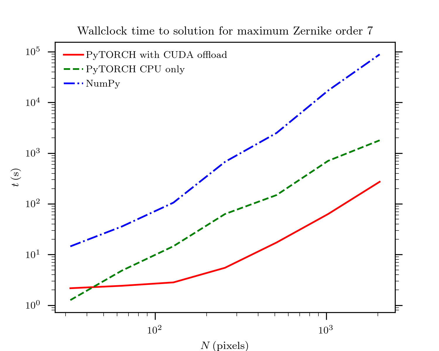
Figure 3: Time to solution as function of the grid size used for modelling the telescope optics. All measurements on a dual-socket Intel Xeon CPU E5-2630 with dual NVidia Tesla K20c GPUs. NumPy: plain CPU-only NumPy implementation; PyTorch CPU only: implementation using PyTorch but without using offloading onto the GPU; PyTorch with CUDA offload: implementation using PyTorch and selecting offloading onto GPUs using the PyTorch CUDA module.

Measured time-to-solution as a function of grid size is shown in Figure 3. It can be seen that the PyTorch implementation is far faster in all configuration, and that the GPU-offloaded execution is faster than the CPU-only execution above grid size $N\geq 64$. For intermediate and large grids ($N>256$) the PyTorch implementation running on CPUs is approximately an order of magnitude faster than the NumPy implementation, while the GPU-offloaded execution is an order of magnitude faster still.

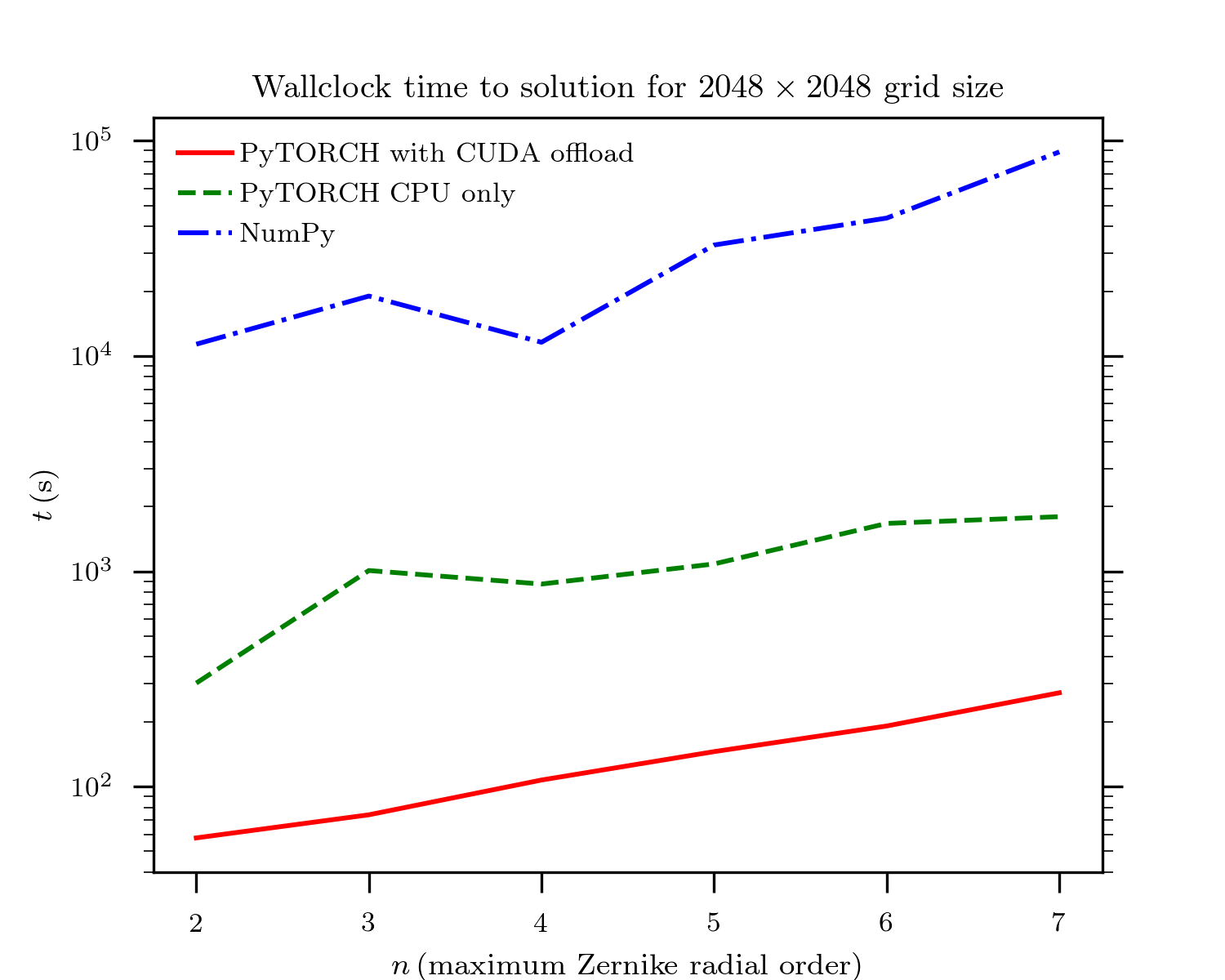
Figure 4: Time to solution as function of the maximum Zernike polynomial order. Measurements were performed as described in Figure 3.

Measured time-to-solution as a function of the number of model parameters is shown in Figure 4. The large improvement in speed by PyTorch is seen to be apparently independent of the model parameters at least in this case.

4 Related work

All of the techniques presented here are well established (although automatic differentiation mostly in specialised applications). The contribution of this paper is illustrate that machine-learning software packages combine them into an easy-to-use system that is also highly applicable for general function minimisation.

The closest related work that I’m aware of is [8], where it is shown that a recurrent neural network (RNN) model is general enough to model the finite difference wave equation propagation in seismic modelling, and therefore that the RNN training software (TensorFlow in this case) can be used to solve such problems (including use of automatic differentiation). In contrast, in this paper I consider more general optimisation and avoid use of a neural network model. Instead basic array operations only are used. Furthermore in this paper focus here is on ease of use and computational efficiency and hence the results for those are presented. Another specialised use of PyTorch for fitting is presented by [9].

NumPy as an easy-to-use and relatively efficient idiom for scientific computing is well documented, e.g., [10]. There a number of automatic differentiation tools available in Python which are studied in relation to function optimisation by [11].

5 Conclusions

I present in this paper some of the advantages that applying PyTorch to general function minimisation in science can bring. These advantages are demonstrated on a realistic scientific problem, maximum-likelihood phase retrieval, where it is shown that two orders of magnitude of improvement in the time-to-solution can be achieved with minimal software engineering effort. Such an improvement in time-to-solution may open new application areas such as optimisation of designs with many more parameters then would by typically used today, or inclusion of fitting of complex models into low-latency control loops.

Importantly, PyTorch programs are about as readable and maintainable as NumPy programs. This is critical many minimisation and fitting applications as subtle error in the model are often masked by counteracting error in the best-fitting parameters.

References

- [1] J. Nocedal and S. J. Wright, Numerical Optimization, 2nd ed. New York: Springer, 2006.
- [2] T. E. Oliphant, “Python for scientific computing,” Computing in Science Engineering, vol. 9, no. 3, pp. 10–20, May 2007.
- [3] A. Paszke, S. Gross, S. Chintala, G. Chanan, E. Yang, Z. DeVito, Z. Lin, A. Desmaison, L. Antiga, and A. Lerer, “Automatic differentiation in pytorch,” 2017.
- [4] A. Gunes Baydin, B. A. Pearlmutter, A. Andreyevich Radul, and J. M. Siskind, “Automatic differentiation in machine learning: a survey,” ArXiv e-prints, Feb. 2015.
- [5] B. Nikolic, R. E. Hills, and J. S. Richer, “Measurement of antenna surfaces from in- and out-of-focus beam maps using astronomical sources,” A&A, vol. 465, pp. 679–683, Apr. 2007.
- [6] P. Sarder and A. Nehorai, “Deconvolution methods for 3-d fluorescence microscopy images,” vol. 23, pp. 32 – 45, 06 2006.
- [7] C. Correia, J. Veran, O. Guyon, and C. Clergeon, “Wave-front reconstruction for the non-linear curvature wave-front sensor,” in Proceedings of the Third AO4ELT Conference, S. Esposito and L. Fini, Eds. Firenze: INAF - Osservatorio Astrofisico di Arcetri, 2013.
- [8] A. Richardson, “Seismic Full-Waveform Inversion Using Deep Learning Tools and Techniques,” ArXiv e-prints, Jan. 2018.
- [9] F. de Avila Belbute-Peres and J. Z. Kolter, “A modular differentiable rigid body physics engine,” in Deep Reinforcement Learning Symposium, ser. NIPS 2017, 2017.
- [10] S. van der Walt, S. C. Colbert, and G. Varoquaux, “The numpy array: A structure for efficient numerical computation,” Computing in Science Engineering, vol. 13, no. 2, pp. 22–30, March 2011.
- [11] A. Turkin and A. Thu, “Benchmarking Python Tools for Automatic Differentiation,” ArXiv e-prints, Jun. 2016.