The global optimum of shallow neural network is attained by ridgelet transform

Abstract

We prove that the global minimum of the backpropagation (BP) training problem of neural networks with an arbitrary nonlinear activation is given by the ridgelet transform. A series of computational experiments show that there exists an interesting similarity between the scatter plot of hidden parameters in a shallow neural network after the BP training and the spectrum of the ridgelet transform. By introducing a continuous model of neural networks, we reduce the training problem to a convex optimization in an infinite dimensional Hilbert space, and obtain the explicit expression of the global optimizer via the ridgelet transform.

1 Introduction

Training a neural network is conducted by backpropagation (BP), which results in a high-dimensional and non-convex optimization problem. Despite the difficulty of the optimization problem, deep learning has achieved great success in a wide range of applications such as image recognition (Redmon et al.,, 2016), speech synthesis (van den Oord et al.,, 2016), and game playing (Silver et al.,, 2017). The empirical success of deep learning suggests a conjecture that “all” local minima of the training problem are close or equal to global minima (Dauphin et al.,, 2014; Choromanska et al.,, 2015). Therefore, radical reviews of the shape of loss surfaces are ongoing (Draxler et al.,, 2018; Garipov et al.,, 2018). However, these lines of studies pose strong assumptions such as linear activation (Kawaguchi,, 2016; Hardt and Ma,, 2017), overparameterization (Nguyen and Hein,, 2017), Gaussian data distribution (Brutzkus and Globerson,, 2017), and shallow network, i.e. single hidden layer (Li and Yuan,, 2017; Soltanolkotabi,, 2017; Zhong et al.,, 2017; Du and Lee,, 2018; Ge et al.,, 2018; Soudry and Hoffer,, 2018).

The scope of this study is the shape of the global optimizer itself, rather than the reachability to the global optimum via empirical risk minimization. By recasting the BP training as a variational problem, i.e. an optimization problem in a function space, in the settings of the shallow neural network with an arbitrary activation function and the mean squared error, we present an explicit expression of the global minimizer via the ridgelet transform. By virtue of functional analysis, our result is independent of the parameterization of neural networks.

Figure 1 presents an intriguing example that motivates our study. Both Figures 1(a) and 1(b) were obtained from the same dataset shown in Figure 1(c), and they show similar patterns to each other. However, they were obtained from entirely different procedures: numerical optimization and numerical integration. In the following, we provide a brief explanation of the experiments. See § 3 for more details.

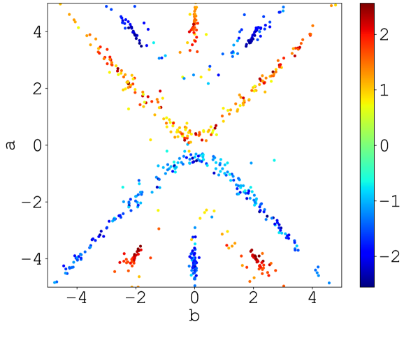
(a) BP trained parameters

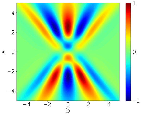
(b) ridgelet spectrum

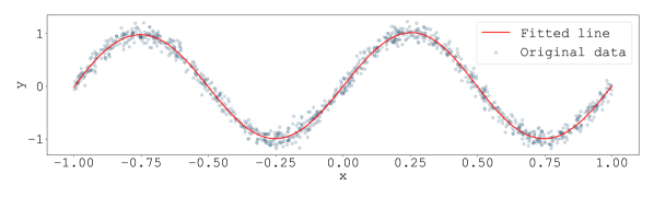
(c) dataset and an example of training results

Figure 1: Motivating example: Scatter plot (a) and ridgelet spectrum (b) were obtained from the same dataset (c) and bear an intriguing resemblance to each other, despite the fact that they were obtained from different procedures—numerical optimization and numerical integration.

Figure 1(a) shows the scatter plot of the parameters $(a_{j},b_{j},c_{j})$ in neural networks $g(x;{\bm{\theta}})=\sum_{j=1}^{p}c_{j}\sigma(a_{j}x-b_{j})$ that had been trained with dataset $D=\{(x_{i},y_{i})\}_{i=1}^{1,000}$. The dataset is composed of uniform random variables $x_{i}$ in $[-1,1]$, and the response variables $\sin 2\pi x_{i}+\varepsilon_{i}$ with Gaussian random noise $\varepsilon_{i}$. We trained $n=1,000$ shallow neural networks. Each network had $p=10$ hidden units with activation $\sigma(z)=\tanh z$. We employed ADAM for the training. The scatter plot presents the $np=10,000$ sets of trained parameters $(a_{j},b_{j},c_{j})$, where $c_{j}$ is visualized in color.

On the other hand, Figure 1(b) shows the spectrum of the (classic) ridgelet transform

$$R[f](a,b):=\int_{{\mathbb{R}}}f(x)\overline{\rho(ax-b)}{\mathrm{d}}x,$$ (1)

of $f(x)=\sin 2\pi x+\varepsilon,\,(x\in[-1,1])$ with a certain ridgelet function $\rho$. (See § 2 for more details on the ridgelet transform.) We calculated the spectrum by using numerical integration, and used the dataset $D$. Therefore, two figures are obtained from the same dataset.

Even though the two figures are obtained from different procedures, both results are $10$-point star shaped. In other words, the BP trained parameters $(a_{j},b_{j},c_{j})$ concentrate in the high intensity areas in the ridgelet spectrum. From this interesting similarity, we can conjecture that the global minimizer has a certain relation to the ridgelet transform.

In this study, we investigate the relation between the BP training problem and the ridgelet transform by reformulating the BP training in a function space, and show that the ridgelet transform can offer the global minimizer of the BP training problem.

2 Preliminaries

We provide several notation and describe the problem formulation. The most important notion is the ‘BP in the function space,’ which plays a key role to formulate our research question.

2.1 Mathematical Notation

$\overline{z}$ denotes the complex conjugate of a complex number $z$. $\widehat{f}$ denotes the Fourier transform $\int f({\bm{x}})e^{-i{\bm{x}}\cdot\bm{\xi}}{\mathrm{d}}{\bm{x}}$ of a function $f$. $\widetilde{f}$ denotes the reflection of a function $f$, i.e. $\widetilde{f}({\bm{x}})=f(-{\bm{x}})$.

$L^{2}(\mu)$ denotes the Hilbert space equipped with inner product $\langle f,g\rangle:=\int f({\bm{x}})\overline{g({\bm{x}})}{\mathrm{d}}\mu({\bm{x}})$. $T^{*}$ denotes the adjoint operator of a linear operator $T$ on a Hilbert space.

${\mathbb{E}}_{X}[f(X)]$ denotes the expectation of a function $f(x)$ with respect to the random variable $X$.

2.2 Problem Settings

Neural Network.  We consider an $m$-in-$1$-out shallow neural network with an arbitrary activation function $\sigma:{\mathbb{R}}\to{\mathbb{C}}$:

$$g({\bm{x}};{\bm{\theta}})=\sum_{j=1}^{p}c_{j}\sigma({\bm{a}}_{j}\cdot{\bm{x}}-b_{j}),\quad{\bm{x}}\in{\mathbb{R}}^{m}$$ (2)

where $p\in{\mathbb{N}}$ is the number of hidden units, $({\bm{a}}_{j},b_{j})\in{\mathbb{R}}^{m}\times{\mathbb{R}}$ are hidden parameters and $c_{j}\in{\mathbb{C}}$ are output parameters. By ${\bm{\theta}}$, we collectively write a set of parameters $\{({\bm{a}}_{j},b_{j},c_{j})\}_{j=1}^{p}$. Here, we remark that the $1$-dimensional output assumption is only for simplicity, and we can easily generalize our results to the multi-dimensional output case. Examples of the activation function are Gaussian, hyperbolic tangent, sigmoidal function and rectified linear unit (ReLU).

Cost Function.  We formulate the BP training as the minimization problem of the mean squared error

$$L({\bm{\theta}})={\mathbb{E}}_{X}|f(X)-g(X;{\bm{\theta}})|^{2}+\Omega({\bm{\theta}}),$$ (3)

with a certain regularization $\Omega$, where $f:{\mathbb{R}}^{m}\to{\mathbb{C}}$ denotes the ground truth function. Here, we remark that this formulation covers any empirical risk function $L_{s}({\bm{\theta}})=\frac{1}{s}\sum_{i=1}^{s}|y_{i}-g({\bm{x}}_{i};{\bm{\theta}})|^{2}+\Omega({\bm{\theta}})$, by choosing the data distribution as an empirical distribution.

2.3 Integral Representation of Neural Network

In order to recast the BP training in the function space, we introduce the integral representation of a neural network:

$$S[\gamma]({\bm{x}}):=\int_{{\mathbb{R}}^{m}\times{\mathbb{R}}}\gamma({\bm{a}},b)\sigma({\bm{a}}\cdot{\bm{x}}-b){\mathrm{d}}\lambda({\bm{a}},b),$$ (4)

where $\gamma:{\mathbb{R}}^{m}\times{\mathbb{R}}\to{\mathbb{C}}$ are the coefficient function, $\sigma:{\mathbb{R}}\to{\mathbb{C}}$ is the activation function employed in (2), and $\lambda$ is the base measure on ${\mathbb{R}}^{m}\times{\mathbb{R}}$.

Brief Description.  Formally speaking, $S[\gamma]$ is an infinite sum of hidden units $\sigma({\bm{a}}\cdot{\bm{x}}-b)$. In the integral representation, all the hidden parameters $({\bm{a}},b)$ are integrated out, and only the output parameter $\gamma({\bm{a}},b)$ is left. In other words, $\gamma({\bm{a}},b)$ indicates which $({\bm{a}},b)$ to use by weighting on them.

Function Class.  In this study, we assume that $\gamma\in L^{2}(\lambda)$, and $\lambda$ be a Borel measure. As described in Proposition 4.2, the base measure $\lambda$ controls the expressive power of neural networks, i.e. the capacity of $\{S[\gamma]\mid\gamma\in L^{2}(\lambda)\}$.

Important Examples.  Two extreme cases are important: (a) $\lambda$ is the Lebesgue measure, and (b) $\lambda$ is a sum of Dirac measures. When $\lambda$ is the Lebesgue measure ${\mathrm{d}}{\bm{a}}{\mathrm{d}}b$, then $S[\gamma]$ can express any $L^{2}$-function (Sonoda and Murata,, 2017). On the other hand, when $\lambda$ is a sum of Dirac measures, then $S[\gamma]$ can express any finite neural network (2). With a slight abuse of notation, write

$$\gamma_{\bm{\theta}}{\mathrm{d}}\lambda=\sum_{j=1}^{p}c_{j}\delta_{({\bm{a}}_{j},b_{j})},$$ (5)

for ${\bm{\theta}}=\{({\bm{a}}_{j},b_{j},c_{j})\}_{j=1}^{p}$, where $\delta_{({\bm{a}},b)}$ denotes the Dirac delta centered at $({\bm{a}},b)$. Then, $S[\gamma_{\bm{\theta}}]({\bm{x}})=\sum_{j=1}^{p}c_{j}\sigma({\bm{a}}_{j}\cdot{\bm{x}}-b_{j})$. In other words, the integral representation is a reparameterization of neural networks, and $\gamma_{\bm{\theta}}$ is the simplest way to connect the integral representation and the ordinary representation.

Advantages.  The integral representation has at least two advantages over the ‘ordinary representation’ (2). The first advantage is that $\gamma_{\bm{\theta}}$ can expressive any distribution of parameters. By virtue of this flexibility, we can identify the scatter plot Figure 1(a) as a point spectrum, and Figure 1(b) as a continuous spectrum.

The second advantage is that the hidden parameters are integrated out, and that the output parameter is the only trainable parameter. Recall that the BP training of ordinary neural networks $g({\bm{x}};{\bm{\theta}})$ is a non-convex optimization problem. The non-convexity is caused by the hidden parameters $({\bm{a}}_{j},b_{j})$, because they are placed in the nonlinear function $\sigma$. At the same time, the non-convexity is never caused by the output parameters $c_{j}$, because they are placed out of $\sigma$. On the other hand, in the integral representation, no trainable parameters are placed in $\sigma$. By virtue of this linearity, the BP training of $S[\gamma]$, which is described later in this section, becomes a convex optimization problem.

Brief History.  Originally, the integral representation and ridgelet transform have been developed to investigate the expressive power of neural networks (Barron,, 1993; Murata,, 1996; Candès,, 1998), and to estimate the approximation errors (Kůrková,, 2012). Recently, it has been applied to synthesize neural networks without BP training, by approximating the integral transform with a Riemannian sum (Sonoda and Murata,, 2014; Bach, 2017a, ; Bach, 2017b, ); to facilitate the inner mechanism of the so-called “black-box” networks (Sonoda and Murata,, 2018), and to estimate the generalization errors of deep neural networks from the decay of eigenvalues (Suzuki,, 2018).

2.4 Ridgelet Transform

We placed the explanation of the ridgelet transform soon after the integral representation, because it is natural to understand the ridgelet transform as a right inverse operator for the integral representation operator.

Let us consider an integral equation $S[\gamma]=f$, where $S$ is an integral representation operator, $f$ is a given function, and $\gamma$ is the unknown function. In the context of neural networks, this equation means a prototype of learning. Namely, to learn $f$ is to find a solution $\gamma$ from the observation $f$. Murata, (1996) and Candès, (1998) discovered that the ridgelet transform provides a particular solution to the equation.

To be precise, when the base measure $\lambda$ of $S$ is the Lebesgue measure ${\mathrm{d}}{\bm{a}}{\mathrm{d}}b$, the function $f$ belongs to $L^{2}({\mathbb{R}}^{m})$, and there exists a ridgelet function $\rho:{\mathbb{R}}\to{\mathbb{C}}$ that satisfies the admissibility condition

$$\int_{\mathbb{R}}\frac{\widehat{\sigma}(\zeta)\overline{\widehat{\rho}(\zeta)}}{|\zeta|^{m}}{\mathrm{d}}\zeta=1,$$ (6)

for the activation function $\sigma$ in $S$, then a particular solution to $S[\gamma]=f$ is given by the ridgelet transform

$$R[f]({\bm{a}},b)=\int_{{\mathbb{R}}^{m}}f({\bm{x}})\overline{\rho({\bm{a}}\cdot{\bm{x}}-b)}{\mathrm{d}}{\bm{x}}.$$ (7)

This is what we call the classic ridgelet transform.

Here, we remark that the solution is not unique. On the contrary, there are an infinite number of different particular solutions, say $\gamma$ and $\gamma^{\prime}$, that satisfy $\gamma\neq\gamma^{\prime}$ but $S[\gamma]=S[\gamma^{\prime}]$. This is immediate from the fact that there are infinitely many different admissible ridgelet functions $\rho$ and $\rho^{\prime}$. Therefore, a single $R$ (specified by $\rho$) is not the exact inverse to $S$, which must satisfy both $SR=\mathrm{Id}$ and $RS=\mathrm{Id}$; but only a right inverse, which only satisfies $SR=\mathrm{Id}$.

In the context of neural networks, the existence of a solution operator $R[f]$ for any function $f$ means the universal approximation property, because a neural network $S[\gamma]$ can express any function $f$ by just letting $\gamma=R[f]$.

As demonstrated in § 3, the ridgelet transform can be computed by numerical integration. See Starck et al., (2010) and Sonoda and Murata, (2017) for more details on ridgelet analysis.

2.5 BP in the Function Space

We rewrite the BP training as the minimization problem of

$$L[\gamma]={\mathbb{E}}_{X}|f(X)-S[\gamma](X)|^{2}+\Omega[\gamma],$$ (8)

with respect to $\gamma\in L^{2}(\lambda)$. This reformulation formally extends the ordinary formulation (3), because $L[\gamma_{\bm{\theta}}]=L({\bm{\theta}})$. In other words, we can understand the ordinary BP problem in the function space, as depicted in Figure 2. We call the minimization problem of $L[\gamma]$ as the BP in the function space. As we mentioned above, by virtue of the linearity of $S$, the BP in the function is reduced as a quadratic programming problem.

Figure 2: Relation between the minimization problems of $L[\gamma]$ and $L({\bm{\theta}})$. The green curve depicts a finite dimensional subspace parameterized by ${\bm{\theta}}$ and embedded in the ground function space. Since $\gamma_{\bm{\theta}}$ is restricted to the subspace, the gradient vector (dashed) is also projected to the tangent space (solid), and thus the gradient descent generally goes off in a different direction from the global minimizer $\gamma^{*}$. If the subspace is curved in the ground function space, there would be multiple local optima such as $\overline{\gamma}_{1},\overline{\gamma}_{2}$ and $\overline{\gamma}_{3}$.

Mathematically speaking, contrary to the finite dimensional optimization problem, existence and uniqueness of the solution depend on the properties of $\gamma,f$ and $S$. For the sake of simplicity, we consider a simple case $\Omega(\gamma)=\beta\|\gamma\|_{L^{2}(\lambda)}^{2}$ with $\beta>0$. In this case, the sufficient condition for the unique existence of the solution is that $S$ is Lipschitz continuous. See Appendix A for more details.

Where are the Local Minima?  The BP training in the function space, i.e. $\min_{\gamma}L[\gamma]$, has a unique global minimum because it is a quadratic programming, while the BP training in the parameter space, i.e. $\min_{\bm{\theta}}L({\bm{\theta}})$, generally has a large number of local minima. This is not a paradox, but simply a matter of parameterization.

In order to figure out the paradox, let us consider performing gradient descent for cost functions $L[\gamma]$ and $L({\bm{\theta}})$. Namely, for $L[\gamma]$, we use functional gradient (Fréchet derivative) $\nabla_{\gamma}L$; and for $L({\bm{\theta}})$, we use partial derivative $\partial_{\bm{\theta}}L$.

Between these two derivatives, a chain-rule holds:

$$\partial_{\bm{\theta}}L[\gamma_{\bm{\theta}}] =\int_{{\mathbb{R}}^{m}\times{\mathbb{R}}}\nabla_{\gamma}L[\gamma_{\bm{\theta}}({\bm{a}},b)]\partial_{\bm{\theta}}\gamma_{\bm{\theta}}({\bm{a}},b){\mathrm{d}}\lambda({\bm{a}},b)$$

$$=\langle\nabla_{\gamma}L[\gamma_{\bm{\theta}}],\partial_{\bm{\theta}}\gamma_{\bm{\theta}}\rangle_{L^{2}(\lambda)}.$$ (9)

In other words, this is a change-of-coordinate from $\gamma$ to ${\bm{\theta}}$.

According to the chain-rule, if the functional gradient vanishes: $\nabla_{\gamma}L[\gamma_{{\bm{\theta}}^{*}}]=0$ at some $\gamma_{{\bm{\theta}}^{*}}$, then the partial derivative also vanishes: $\partial_{\bm{\theta}}L({\bm{\theta}}^{*})=0$. However, the converse is not always true. As depicted in Figure 2, if the partial derivative vanishes: $\partial_{\bm{\theta}}L(\overline{{\bm{\theta}}})=0$ at some $\overline{{\bm{\theta}}}$, then $\gamma_{\overline{{\bm{\theta}}}}$ is simply a local optimizer such as $\overline{\gamma}_{1},\overline{\gamma}_{2}$ and $\overline{\gamma}_{3}$.

2.6 Main Problem

At last, our research problem is formulated as to show

$$\operatornamewithlimits{argmin}_{\gamma\in L^{2}(\lambda)}L[\gamma;f]=R[f],$$ (10)

with a suitable reformulation of ridgelet transform $R$, if needed.

3 Details on Motivating Examples

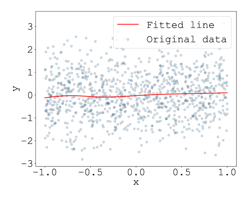
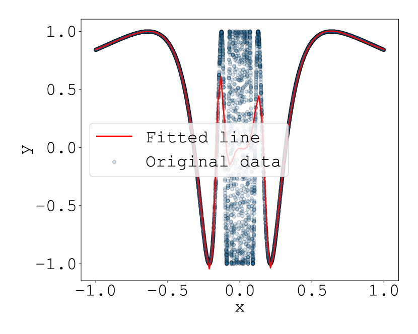
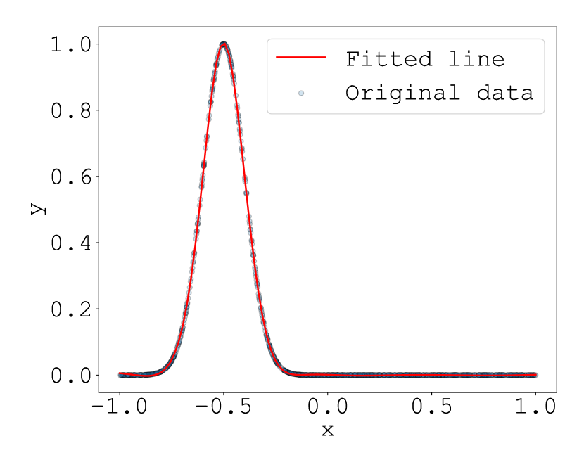
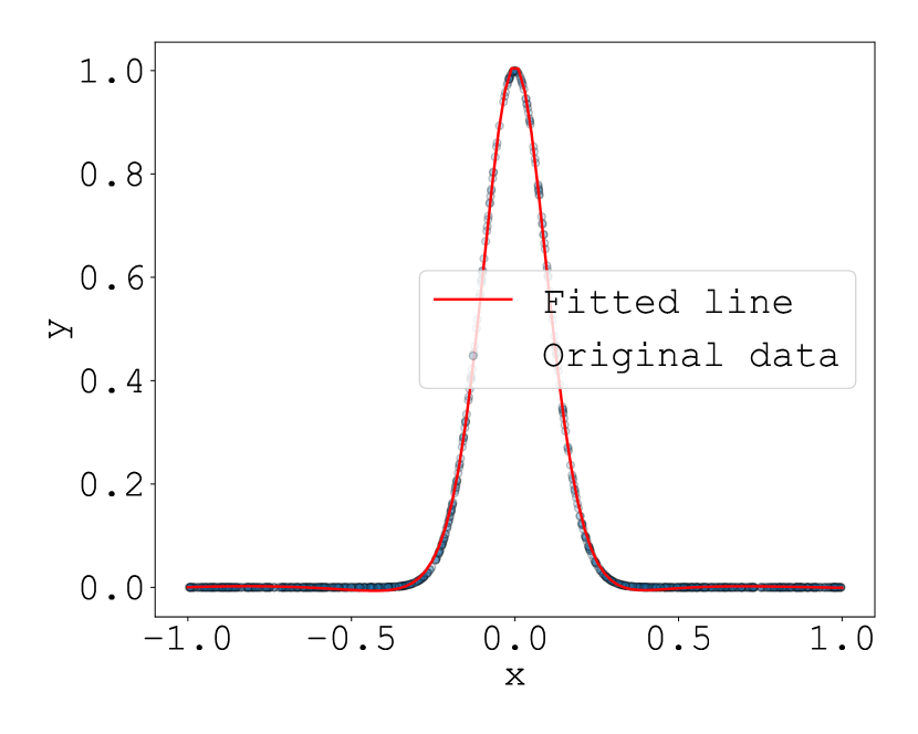
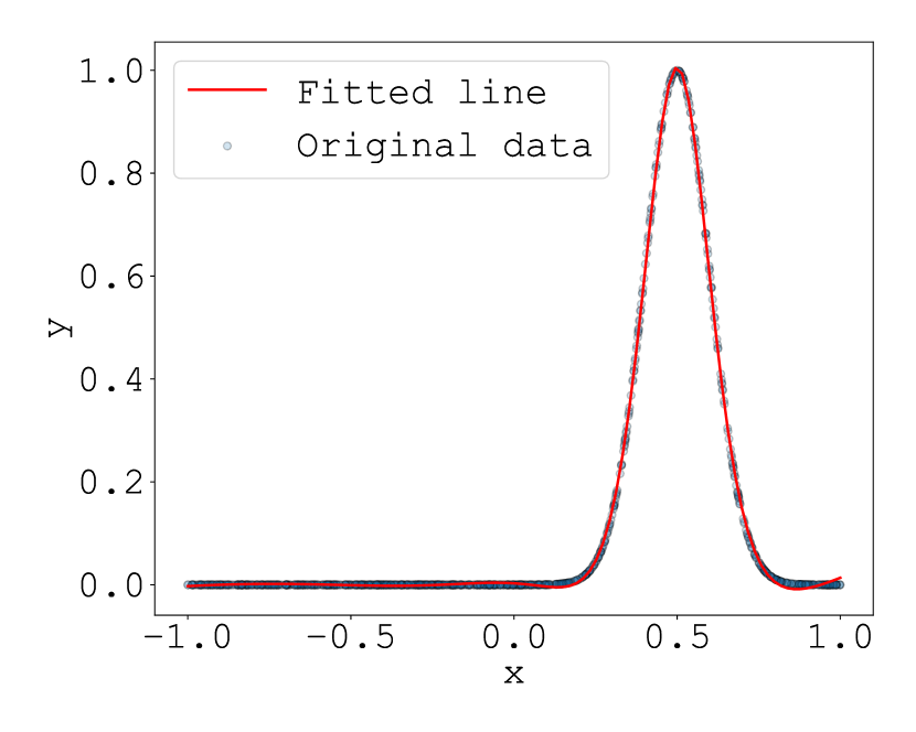
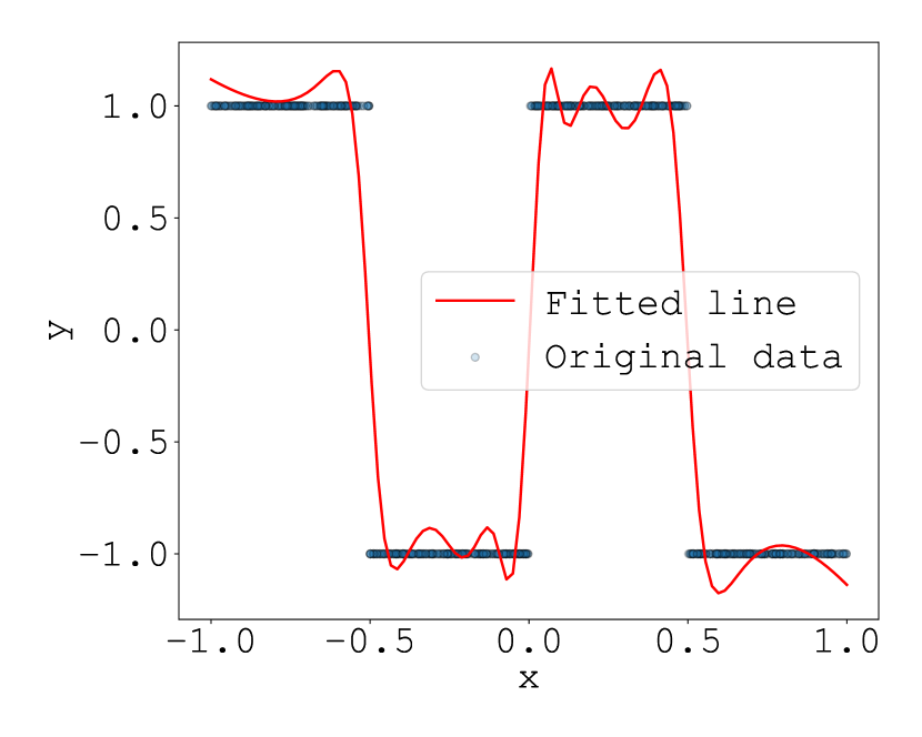
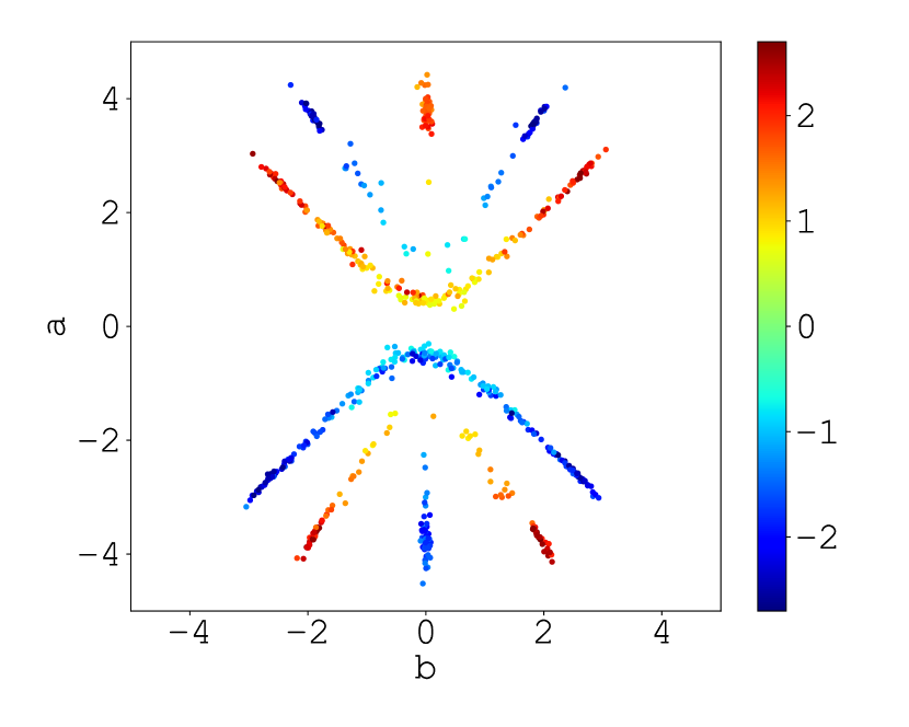
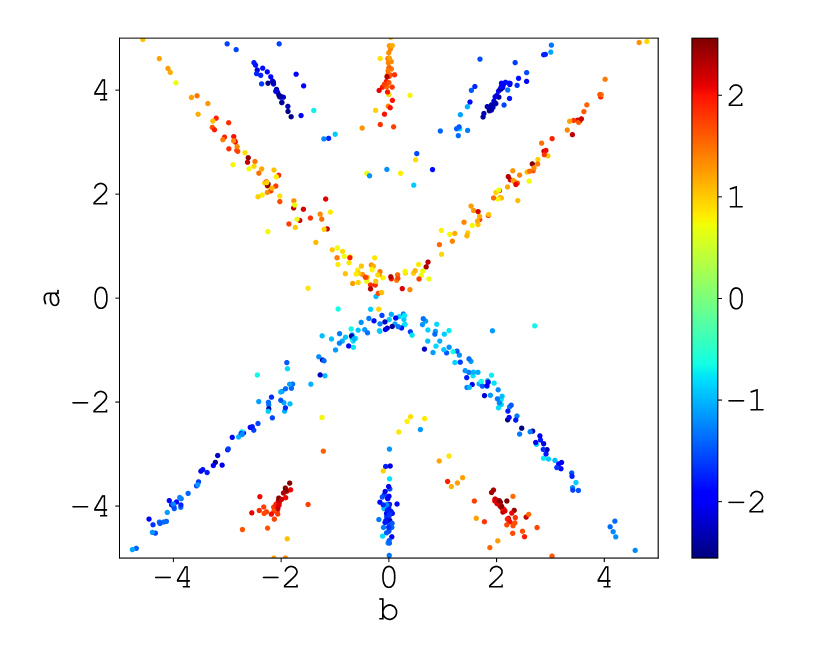
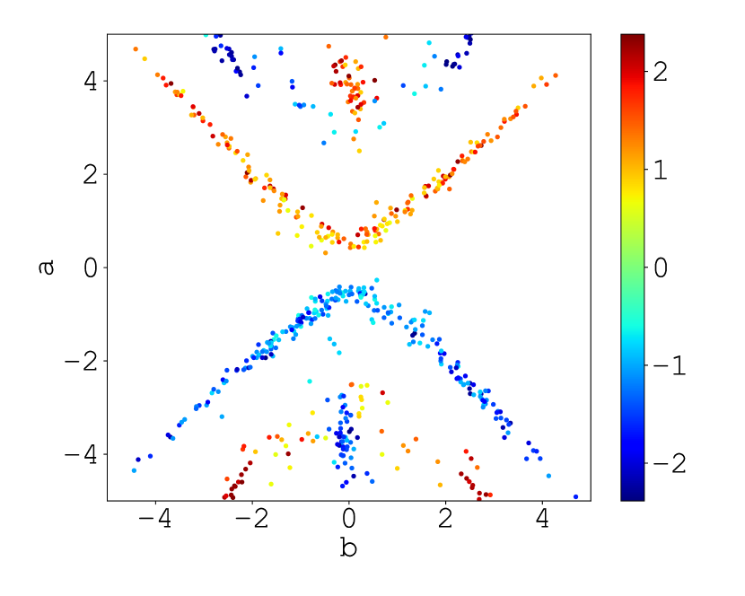
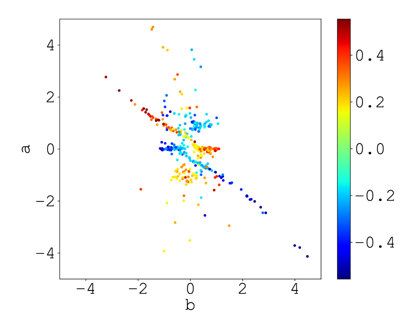
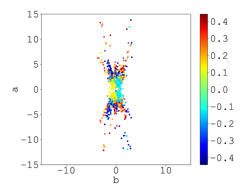
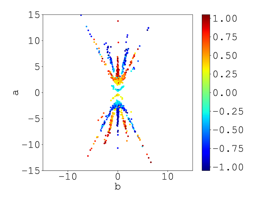
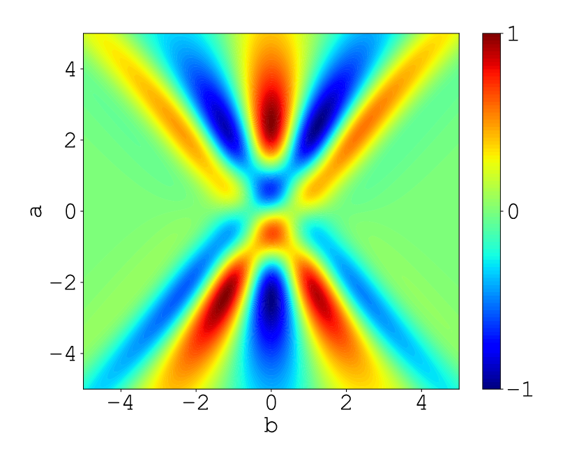
(a)

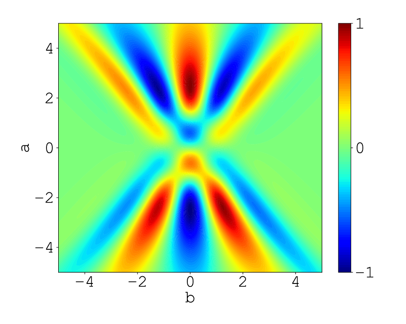
(b)

(c)

(d)

(e)

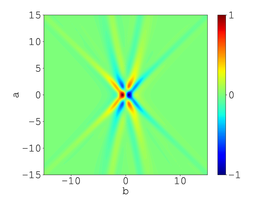
(f)

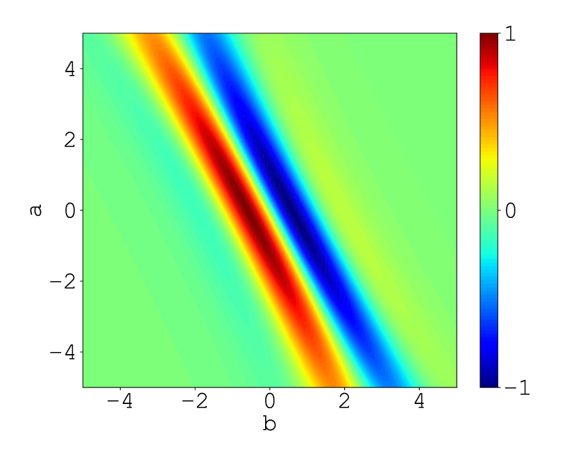
(g)

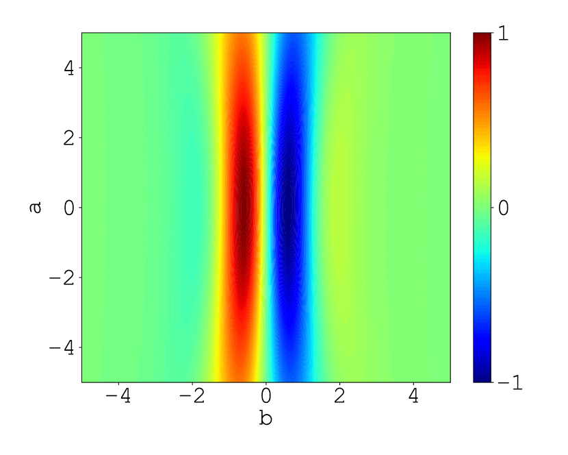
(h)

(i)

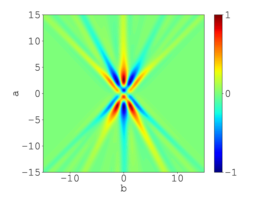
(j)

Figure 3: Experimental results (activation:$\tanh$, optimization:ADAM). (a-c) Sinusoidal Curve (with Noise) $\sigma=0,0.1$ and $1.0$, (d) Gaussian Noise, (e) High Frequency Sinusoidal Curve, (f) Topologist’s Sinusoidal Curve, (g-i) Gaussian Kernel $\mu=-0.5,0.0$ and $.5$, (j) Square Wave. See supplementary materials for all the examples with larger images.

In Figure 1, we have compared the BP trained parameters and the ridgelet spectrum. Here, we explain the details of these experiments and review the results with nine additional datasets and three additional conditions. We note that readers are also encouraged to refer supplementary materials for further results.

3.1 Datasets

We prepared $10$ artificial datasets. For the sake of visualization, all the datasets are $1$-in-$1$-out. We emphasize that our main results described in 4 are valid for any dimension. In the following, $N(\mu,\sigma^{2})$ denotes the normal distribution with mean $\mu$ and variance $\sigma^{2}$, $U(s,t)$ denotes the uniform distribution over the interval $[s,t]$.

Common Settings.  In all the datasets, $x_{i}\sim U(-1,1)$, and except for ‘Topologist’s Sinusoidal Curve’, sample size $s=1,000$.

Sinusoidal Curve.  $y_{i}=\sin 2\pi x_{i}$. We prepared this dataset as a basic example.

Sinusoidal Curve with Gaussian Noise.  $y_{i}=\sin 2\pi x_{i}+\varepsilon_{i},\varepsilon_{i}\sim N(0,\sigma^{2})$ with $\sigma^{2}=0.1^{2}$ and $1^{2}$. We prepared these datasets to examine the effect of noise. By the linearity of ridgelet transform: $R[f+\varepsilon]=R[f]+R[\varepsilon]$, we can expect that the effect will be cancelled out in average.

Gaussian Noise.  $y_{i}\sim N(0,1^{2})$. We prepared this dataset to extract the effect of noise. In theory, the ridgelet spectrum is a random process. Therefore, the visualization result is only a single realization of the random process.

High Frequency Sinusoidal Curve.  $y_{i}=\sin 10\pi x_{i}$. We prepared this dataset to examine the effect of the change in frequency. Since the hidden parameter ${\bm{a}}$ reflects the frequency, we can expect that the spectrum $R[f]({\bm{a}},b)$ will change in ${\bm{a}}$.

Topologist’s Sinusoidal Curve.  $y_{i}=\sin 1/x_{i}$, $s=10,000$. We prepared this dataset to examine the effect of the change in frequency. Compared to sinusoidal curve, it contains an infinitely wide range of frequencies.

Gaussian Kernel.  $y_{i}=\exp(|x_{i}-\mu|^{2}/2)$ with $\mu=-0.5,0,0.5$. We prepared these datasets to examine the effect of the change in location. Since the hidden parameter $b$ reflects the location, we can expect that the spectrum $R[f]({\bm{a}},b)$ will change in $b$.

Square Wave.  $y_{i}=\mathrm{sgn\,}(\sin 2\pi x_{i})$. We prepared this dataset to examine the effect of discontinuity. By the locality of the ridgelet transform, we can expect that the effect is also localized.

3.2 Scatter Plots of BP Trained Parameters

Given a dataset $D=\{(x_{i},y_{i})\}_{i=1}^{s}$, we repeatedly trained $n=1,000$ neural networks $g(x;{\bm{\theta}})=\sum_{j=1}^{p}c_{j}\sigma(a_{j}x-b_{j})$. The training is conducted by minimizing the empirical mean squared error: $L({\bm{\theta}})=\frac{1}{s}\sum_{i=1}^{s}|y_{i}-g(x_{i};{\bm{\theta}})|^{2}$. After the training, we obtained $np$ sets of parameters $(a_{j},b_{j},c_{j})$, and plotted them in the $(a,b,c)$-space. ($c$ is visualized in color.)

We preliminary adjusted the hidden units number $p$ according to the dataset. Otherwise, the plots become noisy, typically because the initial parameters were not moved during the training. If $p$ is too small, the network underfits, and all the parameters become nothing more than noise in the plot. When a network underfits, some $c_{j}$ get extremely large. On the other hand, if $p$ is too large, a large majority of hidden parameters $(a_{j},b_{j})$ remain to be updated, which again become noise in the plot. When a parameter $(a_{j},b_{j})$ remains to be updated, the $c_{j}$ gets extremely small. So, we can judge if the parameters are noise or not, by checking if $c_{j}$ is either extremely large or extremely small. For the sake of visualization, we got rid of those noisy parameters.

We examined the following settings. See supplementary materials for all the results.

Activation Function.  $\tanh$ and ReLU.

Optimization Method.  LBFGS and ADAM.

3.3 Numerical Integration of Ridgelet Spectrum

We employed the classical definition of the ridgelet transform given in (7). As admissible functions $\rho$, we employed

$$\rho(z) =(4z^{2}-2)F(z)-2z, \sigma=\tanh$$ (for )

$$\rho(z) =(12z-8z^{3})F(z)+4z^{2}-4, \sigma=$$ (for ReLU)

where $F(z):=e^{-z^{2}}\int_{0}^{z}e^{w^{2}}{\mathrm{d}}w$ is the Dawson function. See Sonoda and Murata, (2017) for more details on the construction of other admissible functions.

Given the dataset $D=\{(x_{i},y_{i})\}_{i=1}^{s}$, we have conducted a simple Monte Carlo integration at every grid points $(a,b)$:

$$R[f](a,b)\approx\frac{1}{s}\sum_{i=1}^{s}y_{i}\overline{\rho(ax_{i}-b)}\Delta x,$$ (11)

where $\Delta x$ is a normalizing constant (because $x_{i}$ is uniformly distributed). For simplicity, we omitted calculating $\Delta x$, and simply scaled $R[f]$ so that it has value in $[-1,1]$. We remark that more sophisticated methods for the numerical computation of the ridgelet transform has been developed. See Do and Vetterli, (2003) and Sonoda and Murata, (2014) for example.

3.4 Experimental Results

Figure 3 presents the experimental results when the activation function $\sigma$ is $\tanh$ and the optimization method is ADAM. As mentioned in 2.4, there are an infinite number of different ridgelet transforms $R$, and the presented spectra are calculated by just one particular case of $R$. Nevertheless, we can find a visual resemblance in all the cases (a-j).

In (a-c), the three spectra are also similar to each other. As we have expected, the effect of noise has been canceled. The three scatter plot get blurred, as the noise level $\sigma^{2}$ gets increased. In (d), the spectrum presents a single shot of the random field $R[\varepsilon]$. In the scatter plot, parameters accumulated along the line. This is because when $(a,b)$ is on this line, the corresponding base function $\sigma(ax-b)$ tends to be a constant function in the domain $x\in[-1,1]$, as the fitting example depicted in the top. In (e-d), the scatter plots are noisy because the training easily fails, as shown in the training example. We can find some sharp peaks and troughs. In (g-i), we can observe that the location in the real domain is encoded as the angle in the spectrum. In (j), the parameters accumulated in a few sharp lines. These lines encode the locations of discontinuities in the real domain.

4 Theory

We prove the main theorem. All the proofs are given in Appendix B. We fix a locally integrable activation function $\sigma:{\mathbb{R}}\to{\mathbb{C}}$ and a probability measure $\mu$ on ${\mathbb{R}}^{m}$. We remark that the boundedness is not critical but just for simplicity. We can treat unbounded activation functions with small modifications employed in Sonoda and Murata, (2017). We define a positive definite kernel $K$ on $\mathbb{R}^{m}\times\mathbb{R}$ by

$$K\!\left(({\bm{a}},b),({\bm{a}}^{\prime},b^{\prime})\right):=\int_{{\mathbb{R}}^{m}}\sigma({\bm{a}}\cdot{\bm{x}}-b)\overline{\sigma({\bm{a}}^{\prime}\cdot{\bm{x}}-b^{\prime})}{\mathrm{d}}\mu({\bm{x}}).$$ (12)

Let $\mathcal{P}:=\left\{\text{finite Borel measure on }\mathbb{R}^{m}\times\mathbb{R}\right\}$ and assume $\lambda\in\mathcal{P}$. For example, the Dirac measure $\delta_{({\bm{a}},b)}$ with support on $({\bm{a}},b)$ is contained in $\mathcal{P}$.

4.1 Integral Representation of Neural Network

Here, we investigate the properties of integral representation operator $S:L^{2}(\lambda)\to L^{2}(\mu)$.

Proposition 4.1.

The operator $S$ is a bounded linear operator, more precisely, for any $\gamma\in L^{2}(\lambda)$, we have $||S[\gamma]||_{L^{2}(\mu)}\leq||K||_{L^{2}(\lambda\otimes\lambda)}^{1/2}\cdot||\gamma||_{L^{2}(\lambda)}$.

Let $k$ be a positive definite kernel on ${\mathbb{R}}^{m}$ defined by

$$k({\bm{x}},{\bm{y}}):=\int_{{\mathbb{R}}^{m}}\sigma({\bm{a}}\cdot{\bm{x}}-b)\overline{\sigma({\bm{a}}\cdot{\bm{y}}-b)}\,{\mathrm{d}}\lambda({\bm{a}},b).$$ (13)

Let $H$ be the reproducing kernel Hilbert space (RKHS) associated with $k$. We note that $H\subset L^{2}(\mu)$. Then we have

Proposition 4.2.

The image of $S$ is $H$.

Proposition 4.2 means that the representation ability of $S$ is described by the RKHS $H$. If $k$ is a universal kernel (cc-universal in the sense in Sriperumbudur et al., (2010)), the RKHS $H$ can approximate any compact support function in $L^{2}(\mu)$, which is just the universal approximation property of neural networks in $L^{2}(\mu)$ for arbitrary probability distribution $\mu$. Actually, under mild condition, we can make $k$ a universal kernel as follows:

Theorem 4.3.

Let $A>0$ be a (large) positive number. Let $\nu\in L^{1}({\mathbb{R}}^{m})$. Assume that $\sigma$ is a non-constant periodic function with period $2A$, i.e. $\sigma(x+2A)=\sigma(x)$. We also impose one of the two conditions: (1) ${\rm supp}(\nu)={\mathbb{R}}^{m}$ or (2) $0\in{\rm supp}(\nu)$ and $\#\{\widehat{\sigma}(n)\neq 0\}=\infty$, where $\widehat{\sigma}(n)=(2A)^{-1}\int_{[-A,A]}\sigma(x)e^{\pi inx/A}dx$. Then $\lambda=\nu({\bm{a}})\mathbf{1}_{[-A,A]}(b){\mathrm{d}}{\bm{a}}{\mathrm{d}}b\in\mathcal{P}$ induces a universal kernel $k$.

Note that in a real world problems, we can use a periodic function $\sum_{n=-\infty}^{\infty}\sigma(x-2nA)\mathbf{1}_{[(n-1)A,(n+1)A]}$ with sufficiently large $A>0$ as an alternative activation function. Thus the condition of periodicity for $\sigma$ is not harmful. In particular, we can deal with ReLU.

4.2 Ridgelet Transform

Here, we introduce a modified version of the ridgelet transform, which attains the global minimum of the BP training problem.

Let $\lambda\in\mathcal{P}$ and let $\rho\in L^{2}(\mu\otimes\lambda)$. Then we define the Ridgelet transform with respect to $\rho$ as a linear operator $R_{\rho}:L^{2}(\mu)\rightarrow L^{2}(\lambda)$ defined by

$$R_{\rho}[f]({\bm{a}},b):=\int_{\mathbb{R}^{m}}f({\bm{x}})\rho({\bm{x}},({\bm{a}},b))\,{\mathrm{d}}\mu({\bm{x}}).$$ (14)

We note this definition includes the classic definition when $\rho({\bm{x}},({\bm{a}},b))=\rho({\bm{a}}\cdot{\bm{x}}-b)$ and ${\mathrm{d}}\mu({\bm{x}})={\mathrm{d}}{\bm{x}}$.

Proposition 4.4.

The ridgelet transform $R_{\rho}$ is a bounded linear operator, more precisely, $||R_{\rho}[f]||_{L^{2}(\lambda)}\leq||f||_{L^{2}(\mu)}||\rho||_{L^{2}(\mu\otimes\lambda)}$.

The adjoint $S^{*}$ of $S$ is described by the ridgelet transform:

Proposition 4.5.

We have $R_{\rho_{\sigma}}=S^{*}$, where $\rho_{\sigma}({\bm{x}},({\bm{a}},b)):=\sigma({\bm{a}}\cdot{\bm{x}}-b)$.

Let $T:L^{2}(\lambda)\rightarrow L^{2}(\lambda)$ be the integral transform with respect to $K$, namely,

$$T[\gamma]({\bm{a}},b):=\int_{{\mathbb{R}}^{m}\times{\mathbb{R}}}\gamma({\bm{a}}^{\prime},b^{\prime})K(({\bm{a}},b),({\bm{a}}^{\prime},b^{\prime}))\,{\mathrm{d}}\lambda({\bm{a}}^{\prime},b^{\prime}).$$ (15)

Then we have the following proposition:

Proposition 4.6.

We have $T=S^{*}S$.

4.3 Main Result

For $f\in L^{2}(\mu)$ and $\beta>0$, let $L[\gamma;f,\beta]:=||S[\gamma]-f||_{L^{2}(\mu)}^{2}+\beta||\gamma||_{L^{2}(\lambda)}^{2}$ be the risk function for the integral representation of neural networks with respect to $\lambda$, then we have the following theorem:

Theorem 4.7.

For $f\in L^{2}(\mu)$ and $\beta>0$, there exists a function $\rho^{*}$ on ${\mathbb{R}}\times({\mathbb{R}}^{m}\times{\mathbb{R}})$ such that $R_{\rho^{*}}[f]$ attains the unique minimum of the minimization problem $\min_{\gamma\in L^{2}(\lambda)}L(f,\beta;\gamma)$. Moreover $\rho^{*}$ satisfies

$$(\beta+T)\rho^{*}({\bm{x}},\cdot)=\sigma_{\bm{x}},$$ (16)

where $\sigma_{\bm{x}}({\bm{a}},b)=\sigma({\bm{a}}\cdot{\bm{x}}-b)$.

In the classic case when ${\mathrm{d}}\lambda={\mathrm{d}}{\bm{a}}{\mathrm{d}}b$ and ${\mathrm{d}}\mu({\bm{x}})={\mathrm{d}}{\bm{x}}$, the solution $\rho^{*}$ is given by $\rho_{\bm{x}}({\bm{a}},b)=(\beta+1)^{-1}\rho({\bm{a}}\cdot{\bm{x}}-b)$ with any admissible $\rho$, which results in a shrink version of the classic ridgelet transform $(\beta+1)^{-1}R_{\rho}$. See Appendix B.8 for a sketch of proof.

5 Conclusion

We have shown that the global minimizer of the BP training problem is given by the ridgelet transform. In order to treat the scatter plot of hidden parameters, such as Figure 1(a), we introduced the integral representation of neural networks, and reformulated the BP training problem in the Hilbert space of coefficient functions, i.e. $\min_{\gamma\in L^{2}(\lambda)}L[\gamma]$. As a result, the BP training problem was reduced to the quadratic programming, without harming the generality of activation functions. At last, we have successfully discovered a modified version of the ridgelet transform that attains the global minimum. In the classic setting, the modified transform simplifies to a shrink ridgelet transform. By virtue of functional analysis, our formulation is independent of the parameterization of neural networks, which would contribute to the geometric understanding of neural networks. Extensions to general risk functions and deep networks, and applications to the analysis of local minima will be our important future works.

Appendix A Optimization Problem in Hilbert spaces

Let $H_{0},H_{1}$ be Hilbert spaces endowded with the inner products $\langle\cdot,\cdot\rangle_{0}$ and $\langle\cdot,\cdot\rangle_{1}$, respectively, and $A:H_{0}\to H_{1}$ be a densely defined closed linear operator.

For a given $f\in H_{1}$, we find $g\in H_{0}$ satisfying

$$Ag=f.$$

For this problem, we have the following.

Proposition A.1.

Let $f\in H_{1}$. Then for every $\beta>0$, we have

$$\operatornamewithlimits{argmin}_{g\in H_{0}}\left(\|Ag-f\|_{1}^{2}+\beta\|g\|_{0}^{2}\right)=(\beta+A^{*}A)^{-1}A^{*}f,$$

where $A^{*}:H_{1}\rightarrow H_{0}$ denotes the adjoint operator of $A$.

Proof.

A direct computation gives

$$\|Ag-f\|_{1}^{2}+\beta\|g\|_{0}^{2}$$

$$=\langle Ag,Ag\rangle_{1}-2\Re\langle Ag,f\rangle_{1}+\langle f,f\rangle_{1}+\beta\langle g,g\rangle_{0}$$

$$=\langle\sqrt{\beta+A^{*}A}g,\sqrt{\beta+A^{*}A}g\rangle_{0}-2\Re\langle\sqrt{\beta+A^{*}A}g,\sqrt{\beta+A^{*}A}^{-1}A^{*}f\rangle_{0}+\langle f,f\rangle_{1}$$

$$=\|\sqrt{\beta+A^{*}A}g-\sqrt{\beta+A^{*}A}^{-1}A^{*}f\|_{0}^{2}+({\rm nonnegative}).$$

Therefore, the objective functional attains the minimum at $g^{*}=(\beta+A^{*}A)^{-1}A^{*}f$. ∎

Appendix B Proofs

B.1 Proposition 4.1

Proof.

Let $\gamma\in L^{2}(\lambda)$. Then we have

$$||S[\gamma]||_{L^{2}(\mu)}^{2}$$

$$=\iiint\gamma({\bm{a}},b)\overline{\gamma({\bm{a}}^{\prime},b^{\prime})}\sigma({\bm{a}}\cdot x-b)\overline{\sigma({\bm{a}}^{\prime}\cdot x-b^{\prime})}{\mathrm{d}}\lambda({\bm{a}},b){\mathrm{d}}\lambda({\bm{a}}^{\prime},b^{\prime})d\mu(x)$$

$$=\int\gamma({\bm{a}},b)\overline{\gamma({\bm{a}}^{\prime},b^{\prime})}K(({\bm{a}},b),({\bm{a}}^{\prime},b^{\prime})){\mathrm{d}}\lambda\otimes{\mathrm{d}}\lambda(({\bm{a}},b),({\bm{a}}^{\prime},b^{\prime}))$$

$$\leq||\gamma||_{L^{2}(\lambda)}^{2}||K||_{L^{2}(\lambda\otimes\lambda)}.$$

Here, in the last line, we use the Cauchy-Schwarz inequality. ∎

B.2 Proposition 4.2

Proof.

Let $\sigma_{\bm{x}}({\bm{a}},b):=\sigma({\bm{a}}\cdot{\bm{x}}-b)$. Let $H^{\prime}\subset L^{2}(\lambda)$ be a closure of the linear subspace generated by $\{\sigma_{\bm{x}}\}_{{\bm{x}}\in{\mathbb{R}}^{m}}$. By definition, we have $S[\sigma_{\bm{x}}]=k({\bm{x}},\cdot)$ and $\langle\sigma_{\bm{x}},\sigma_{\bm{y}}\rangle_{L^{2}(\lambda)}=k({\bm{x}},{\bm{y}})$. Thus, $S$ induces an isomorphism between Hilbert spaces $H^{\prime}$ and $H$, in particular, the image of $S$ is $H$. ∎

B.3 Theorem 4.3

Proof.

Let $I:=[-A,A]$. Since $\sigma$ is a periodic function, we have a Fourier series expansion of $\sigma$: $\sigma(x)=\sum_{n\in\mathbb{Z}}\widehat{\sigma}(n)e^{\pi in/A}$. Then we have

$$k({\bm{x}},{\bm{y}}) =\int_{{\mathbb{R}}^{m}\times I}\sigma({\bm{a}}\cdot{\bm{x}}-b)\sigma({\bm{a}}\cdot{\bm{y}}-b)\nu({\bm{a}}){\mathrm{d}}{\bm{a}}{\mathrm{d}}b$$

$$=\int_{{\mathbb{R}}^{m}}(\sigma*\widetilde{\sigma})({\bm{a}}\cdot({\bm{x}}-{\bm{y}}))\nu({\bm{a}}){\mathrm{d}}{\bm{a}},$$

$$=\int_{{\mathbb{R}}^{m}}\sum_{n\in\mathbb{Z}}|\widehat{\sigma}(n)|^{2}e^{2\pi in{\bm{a}}\cdot({\bm{x}}-{\bm{y}})}\nu({\bm{a}}){\mathrm{d}}{\bm{a}}$$

$$=|a_{0}|^{2}||\nu||_{L^{1}}+\int_{{\mathbb{R}}^{m}}\underbrace{\sum_{n\in\mathbb{Z}\setminus\{0\}}\frac{|\widehat{\sigma}(n)|^{2}}{|n|^{m}}\nu\left(\frac{{\bm{a}}}{n}\right)}_{=:q({\bm{a}})}e^{\pi i{\bm{a}}\cdot({\bm{x}}-{\bm{y}})/A}{\mathrm{d}}{\bm{a}}.$$

Here, $\sigma*\widetilde{\sigma}(x):=\int_{[-A,A]}\sigma(t)\sigma(t-x)dt$. Since we assume ${\rm supp}(\nu)={\mathbb{R}}^{m}$, or $\#\{n~{}|~{}\widehat{\sigma}(n)\neq 0\}=\infty$, the support of the function $q$ is ${\mathbb{R}}^{m}$. Therefore, we see that $k$ is universal (see Section 3.2. of (Sriperumbudur et al.,, 2010)). ∎

B.4 Proposition 4.4

Proof.

Let $f\in L^{2}(\mu)$. Then we have

$$||R_{\rho}[f]||_{L^{2}(\lambda)}^{2}$$

$$=\iiint f(x)f(y)\rho(x,({\bm{a}},b))\rho(y,({\bm{a}},b)){\mathrm{d}}\mu(x){\mathrm{d}}\mu(y){\mathrm{d}}\lambda({\bm{a}},b)$$

$$=\int f(x)f(y)\int\rho(x,({\bm{a}},b))\rho(y,({\bm{a}},b)){\mathrm{d}}\lambda({\bm{a}},b){\mathrm{d}}\mu\otimes{\mathrm{d}}\mu(x,y)$$

$$\leq||f||_{L^{2}(\mu)}^{2}||\rho||^{2}_{L^{2}(\mu\otimes\lambda)}.$$

In the last line, we use the Cauchy-Schwartz inequality twice. ∎

B.5 Proposition 4.5

Proof.

It suffices to prove that $\langle R_{\rho_{\sigma}}[f],\gamma\rangle_{L^{2}(\lambda)}=\langle f,S[\gamma]\rangle_{L^{2}(\mu)}$. By straightforward computation, we have

$$\langle R_{\rho_{\sigma}}[f],\gamma\rangle_{L^{2}(\lambda)}$$

$$=\iint f({\bm{x}})\sigma({\bm{a}}\cdot{\bm{x}}-b)\overline{\gamma({\bm{a}},b)}\,d\mu({\bm{x}})d\lambda({\bm{a}},b)$$

$$=\int f({\bm{x}})\int\overline{\gamma({\bm{a}},b)}\sigma({\bm{a}}\cdot{\bm{x}}-b)d\lambda({\bm{a}},b)d\mu({\bm{x}})$$

$$=\langle f,S[\gamma]\rangle_{L^{2}(\mu)}.$$

Thus we have $R_{\rho_{\sigma}}=S^{*}$. ∎

B.6 Proposition 4.6

Proof.

By Proposition 4.5, we have

$$S^{*}S\gamma({\bm{a}},b)$$

$$=\iint\gamma({\bm{a}}^{\prime},b^{\prime})\sigma({\bm{a}}^{\prime}\cdot{\bm{x}}-b^{\prime})\sigma({\bm{a}}\cdot{\bm{x}}-b){\mathrm{d}}\lambda({\bm{a}}^{\prime},b^{\prime}){\mathrm{d}}\mu({\bm{x}})$$

$$=T[\gamma]({\bm{a}},b).\qed$$

B.7 Theorem 4.7

Proof.

Since $\beta\mathrm{Id}+T$ is an isomorphism, we define $\rho^{*}({\bm{x}},({\bm{a}},b)):=\left((\beta+T)^{-1}\sigma_{\bm{x}}\right)({\bm{a}},b)$. By Proposition A.1, the minimizer $\gamma^{*}$ that attains $\min_{\gamma\in L^{2}(\lambda)}L(f,\beta;\gamma)$ is explicitly given as $(\beta+S^{*}S)^{-1}S^{*}f$. By Proposition 4.5 and Proposition 4.6, it suffices to prove that $(\beta+T)R_{\rho^{*}}=R_{\rho_{\sigma}}$, but it follows from simple computation. ∎

B.8 Remark on Theorem 4.7

Let $\rho$ be an arbitrary admissible, namely, $\int_{{\mathbb{R}}}\widehat{\sigma}(\zeta)\overline{\widehat{\rho}{\zeta}}|\zeta|^{-m}{\mathrm{d}}\zeta=(2\pi)^{-(m-1)}$. Then,

$$T[\rho_{\bm{x}}]({\bm{a}},b)$$

$$=\int\rho({\bm{a}}^{\prime}\cdot{\bm{x}}-b^{\prime})\int\sigma({\bm{a}}\cdot{\bm{x}}^{\prime}-b)\overline{\sigma({\bm{a}}^{\prime}\cdot{\bm{x}}^{\prime}-b^{\prime})}{\mathrm{d}}{\bm{a}}^{\prime}{\mathrm{d}}b^{\prime}{\mathrm{d}}{\bm{x}}^{\prime}$$

$$=\int\sigma({\bm{a}}\cdot{\bm{x}}^{\prime}-b)\underbrace{\int\rho({\bm{a}}^{\prime}\cdot{\bm{x}}-b^{\prime})\overline{\sigma({\bm{a}}^{\prime}\cdot{\bm{x}}^{\prime}-b^{\prime})}{\mathrm{d}}{\bm{a}}^{\prime}{\mathrm{d}}b^{\prime}}_{=\delta({\bm{x}}-{\bm{x}}^{\prime})}{\mathrm{d}}{\bm{x}}^{\prime}$$

$$=\sigma_{\bm{x}}({\bm{a}},b).$$

Here, the last equation holds because

$$\int\rho({\bm{a}}\cdot{\bm{x}}-b)\overline{\sigma({\bm{a}}\cdot{\bm{x}}^{\prime}-b)}{\mathrm{d}}{\bm{a}}{\mathrm{d}}b$$

$$=\int(\overline{\widetilde{\rho}}*\sigma)({\bm{a}}\cdot({\bm{x}}-{\bm{x}}^{\prime})){\mathrm{d}}{\bm{a}}$$

$$=(2\pi)^{-1}\int\int_{\mathbb{R}}\overline{\widehat{\rho}(\zeta)}\widehat{\sigma}(\zeta)|\zeta^{-m}|{\mathrm{d}}\zeta e^{i{\bm{a}}\cdot({\bm{x}}-{\bm{x}}^{\prime})}{\mathrm{d}}{\bm{a}}$$

$$=(2\pi)^{-m}\int e^{i{\bm{a}}\cdot({\bm{x}}-{\bm{x}}^{\prime})}{\mathrm{d}}{\bm{a}}=\delta({\bm{x}}^{\prime}-{\bm{x}}).$$

Thus, $\rho^{*}=(\beta+1)^{-1}\rho_{\bm{x}}$ solves the equation.

Acknowledgements

This work was supported by JSPS KAKENHI 18K18113.

Appendix C Further Examples

We present all the experimental results described in § 3. The results are presented as $10$ sets of subfigures. A single set corresponds to one of the $10$ dataset, and it contains a scatter plot of dataset, four scatter plots of parameters, and two spectra.

On the whole, the scatter plots with ADAM are sharper than those with BFGS, and those with ReLU are also sharper than those with $\tanh$. These results suggest the implicit regularization property of both ADAM and ReLU. The scatter plot with ADAM tends to be sharp because less parameters can remain to be trained for the varieties of mini batches. The scatter plot with ReLU tends to be sharp because ReLU is homogeneous and thus two different parameters $(a,b)$ and $(ka,kb)$, where $k>0,$ indicate the same basis function $\sigma(ax-b)$.

(a) dataset

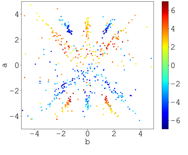
(b) tanh, bfgs

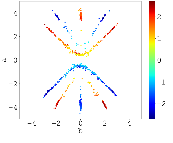
(c) tanh, adam

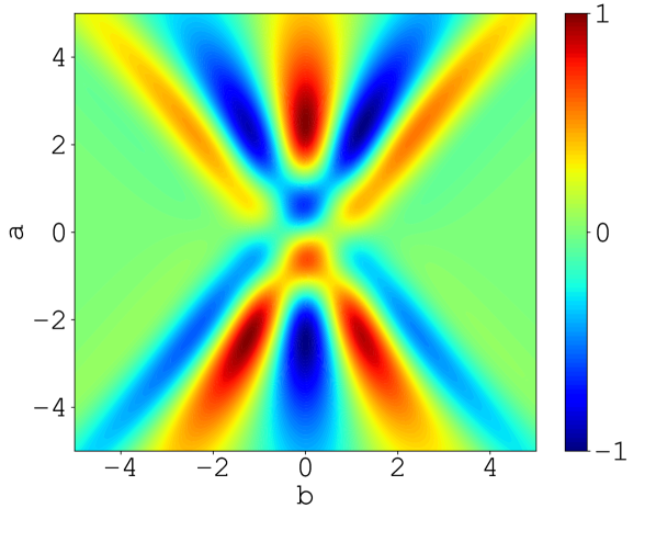
(d) tanh

(e) relu, bfgs

(f) relu, adam

(g) relu

Figure 4: Sinusoidal Curve

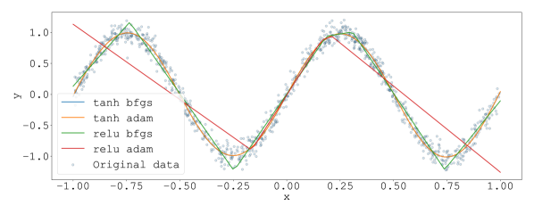
(a) dataset

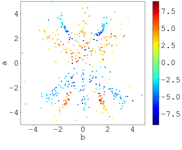
(b) tanh, bfgs

(c) tanh, adam

(d) tanh

(e) relu, bfgs

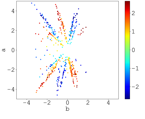
(f) relu, adam

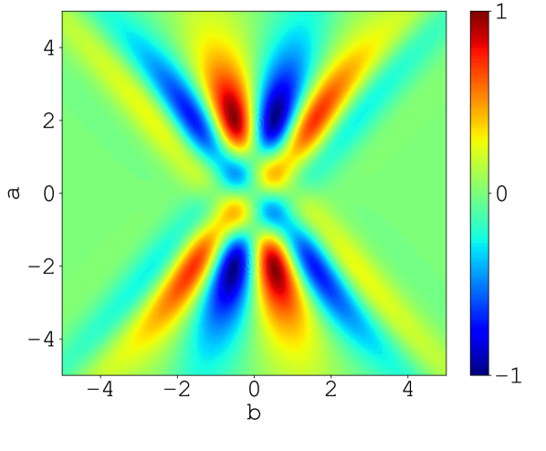
(g) relu

Figure 5: Sinusoidal Curve with Gaussian Noise $N(0,0.1^{2})$

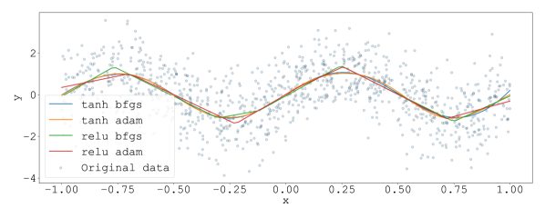
(a) dataset

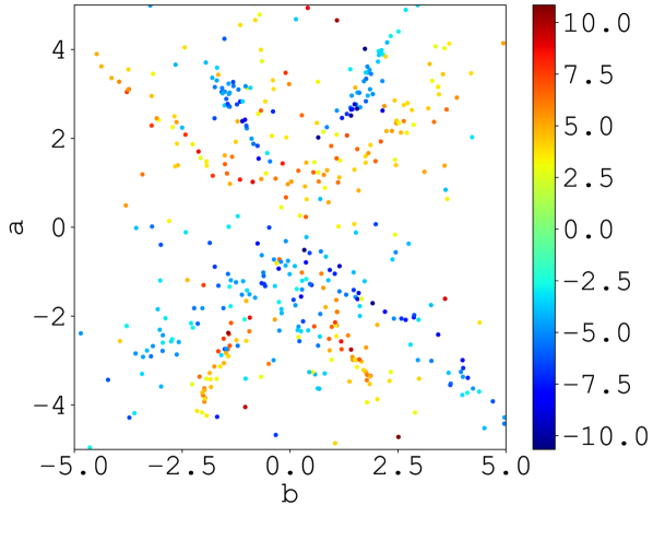
(b) tanh, bfgs

(c) tanh, adam

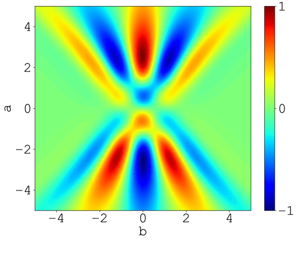
(d) tanh

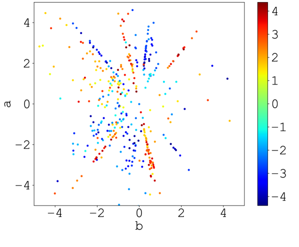
(e) relu, bfgs

(f) relu, adam

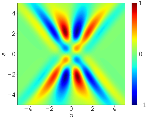
(g) relu

Figure 6: Sinusoidal Curve with Gaussian Noise $N(0,1.0^{2})$

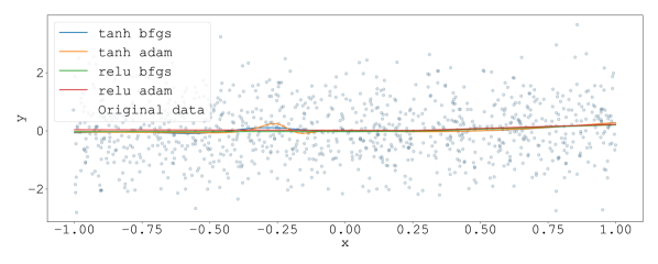
(a) dataset

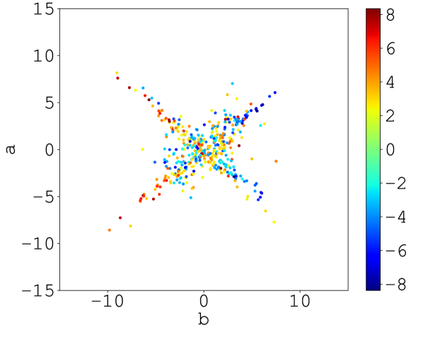
(b) tanh, bfgs

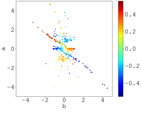
(c) tanh, adam

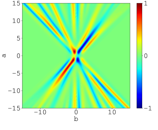
(d) tanh

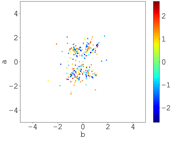
(e) relu, bfgs

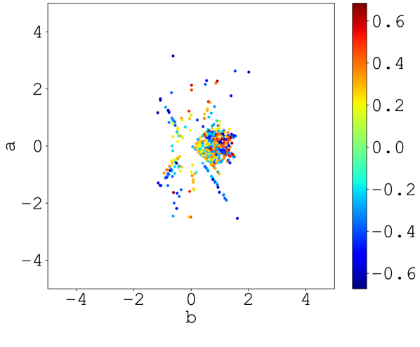
(f) relu, adam

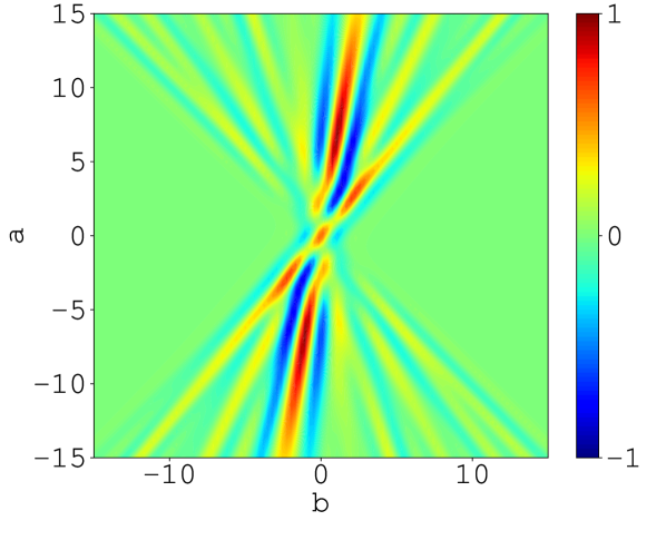
(g) relu

Figure 7: Gaussian Noise $N(0,1.0^{2})$

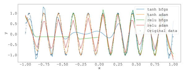
(a) dataset

(b) tanh, bfgs

(c) tanh, adam

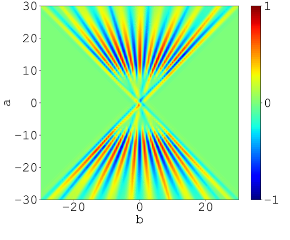
(d) tanh

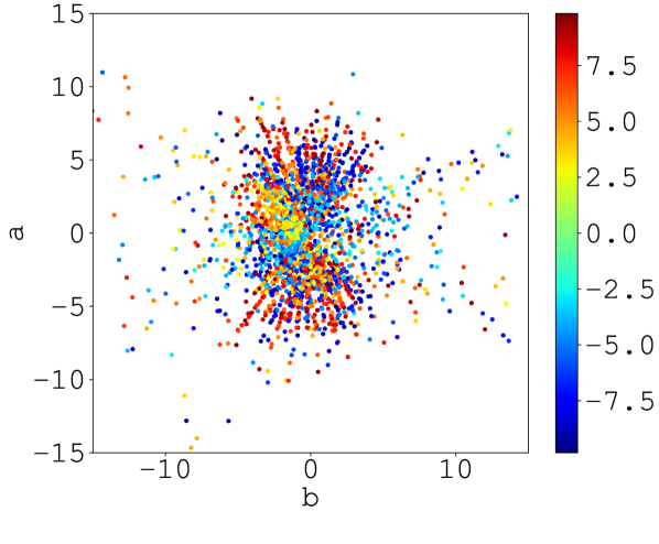
(e) relu, bfgs

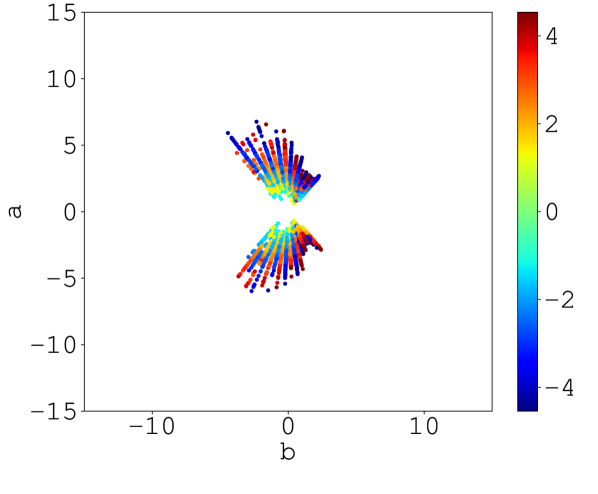
(f) relu, adam

(g) relu

Figure 8: High Frequency Sinusoidal Curve

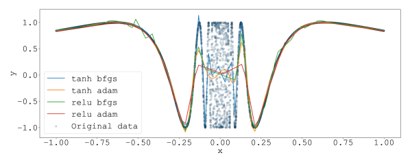
(a) dataset

(b) tanh, bfgs

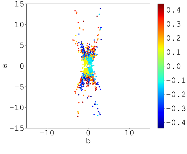
(c) tanh, adam

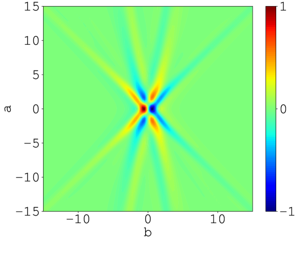
(d) tanh

(e) relu, bfgs

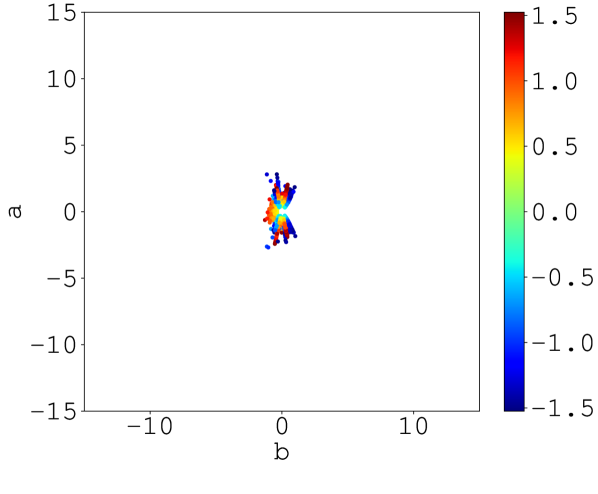
(f) relu, adam

(g) relu

Figure 9: Topologist’s Sinusoidal Curve

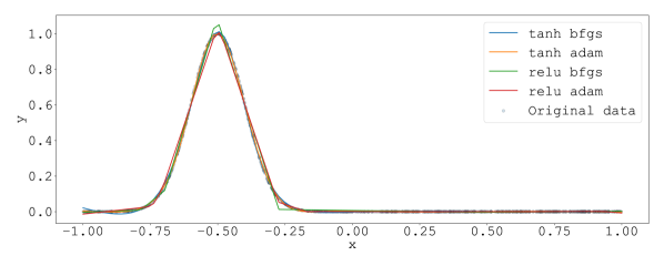
(a) dataset

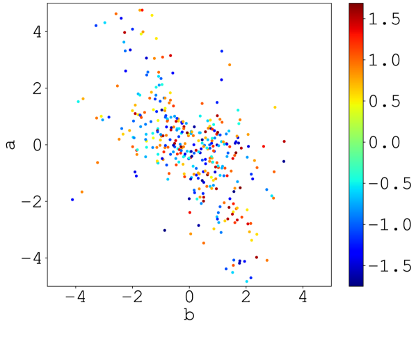
(b) tanh, bfgs

(c) tanh, adam

(d) tanh

(e) relu, bfgs

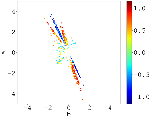
(f) relu, adam

(g) relu

Figure 10: Gaussian Kernel $\mu=-0.5$

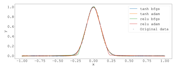
(a) dataset

(b) tanh, bfgs

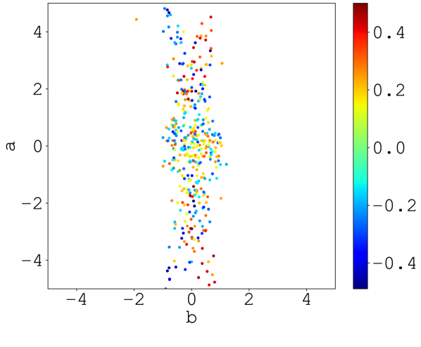
(c) tanh, adam

(d) tanh

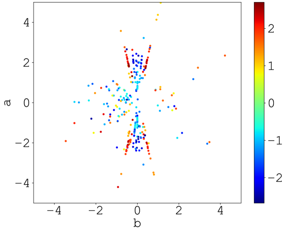
(e) relu, bfgs

(f) relu, adam

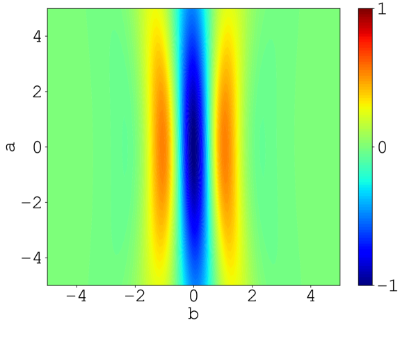
(g) relu

Figure 11: Gaussian Kernel $\mu=0.0$

(a) dataset

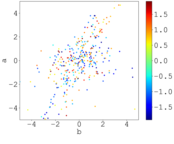
(b) tanh, bfgs

(c) tanh, adam

(d) tanh

(e) relu, bfgs

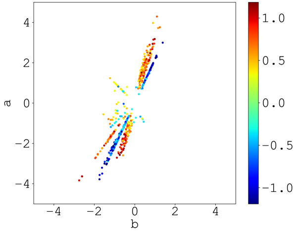
(f) relu, adam

(g) relu

Figure 12: Gaussian Kernel $\mu=0.5$

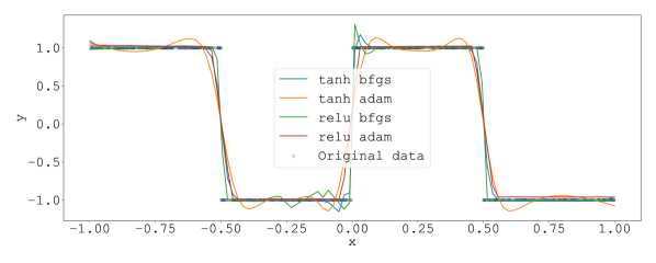
(a) dataset

(b) tanh, bfgs

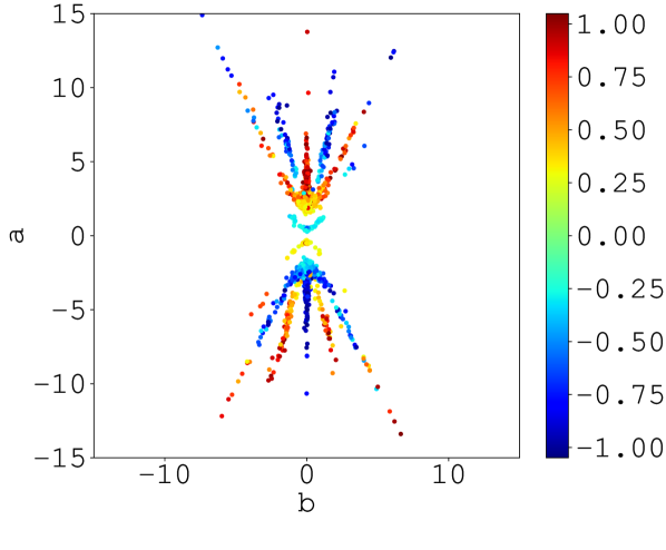
(c) tanh, adam

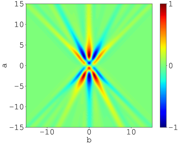
(d) tanh

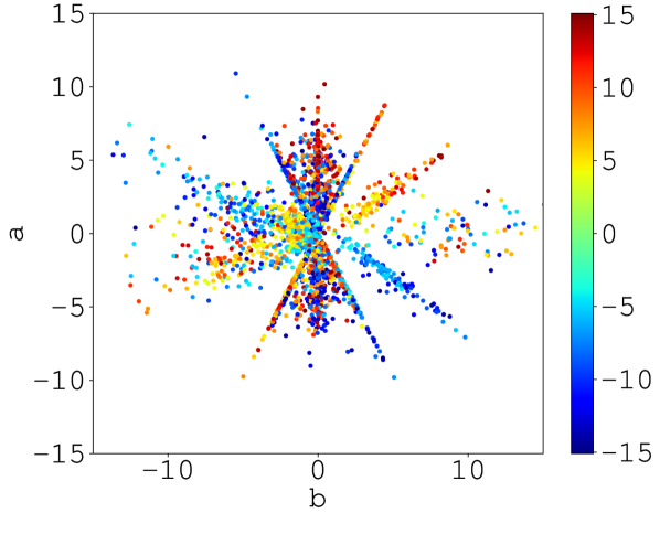
(e) relu, bfgs

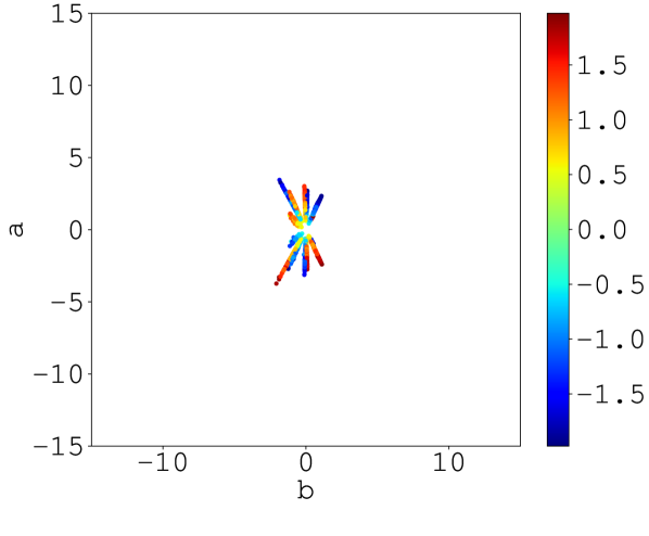
(f) relu, adam

(g) relu

Figure 13: Square Wave

References

- (1) Bach, F. (2017a). Breaking the Curse of Dimensionality with Convex Neural Networks. Journal of Machine Learning Research, 18(19):1–53.
- (2) Bach, F. (2017b). On the Equivalence between Kernel Quadrature Rules and Random Feature Expansions. Journal of Machine Learning Research, 18(21):1–38.
- Barron, (1993) Barron, A. R. (1993). Universal approximation bounds for superpositions of a sigmoidal function. IEEE Transactions on Information Theory, 39(3):930–945.
- Brutzkus and Globerson, (2017) Brutzkus, A. and Globerson, A. (2017). Globally Optimal Gradient Descent for a ConvNet with Gaussian Inputs. In ICML, pages 605–614.
- Candès, (1998) Candès, E. J. (1998). Ridgelets: theory and applications. PhD thesis, Standford University.
- Choromanska et al., (2015) Choromanska, A., Henaff, M., Mathieu, M., Arous, G. B., and LeCun, Y. (2015). The Loss Surfaces of Multilayer Networks. In AISTATS, pages 192–204.
- Dauphin et al., (2014) Dauphin, Y., Pascanu, R., Gulcehre, C., Cho, K., Ganguli, S., and Bengio, Y. (2014). Identifying and attacking the saddle point problem in high-dimensional non-convex optimization. In NIPS, pages 2933–2941.
- Do and Vetterli, (2003) Do, M. N. and Vetterli, M. (2003). The finite ridgelet transform for image representation. IEEE Transactions on Image Processing, 12(1):16–28.
- Draxler et al., (2018) Draxler, F., Veschgini, K., Salmhofer, M., and Hamprecht, F. A. (2018). Essentially No Barriers in Neural Network Energy Landscape. In ICML, pages 1309–1318.
- Du and Lee, (2018) Du, S. S. and Lee, J. D. (2018). On the Power of Over-parametrization in Neural Networks with Quadratic Activation. In ICML, pages 1329–1338.
- Garipov et al., (2018) Garipov, T., Izmailov, P., Podoprikhin, D., Vetrov, D., and Wilson, A. G. (2018). Loss Surfaces, Mode Connectivity, and Fast Ensembling of DNNs. In NIPS, pages 8803–8812.
- Ge et al., (2018) Ge, R., Lee, J. D., and Ma, T. (2018). Learning One-hidden-layer Neural Networks with Landscape Design. In ICLR, pages 1–37.
- Hardt and Ma, (2017) Hardt, M. and Ma, T. (2017). Identity Matters in Deep Learning. In ICLR, pages 1–14.
- Kawaguchi, (2016) Kawaguchi, K. (2016). Deep Learning without Poor Local Minima. In NIPS, pages 586–594.
- Kůrková, (2012) Kůrková, V. (2012). Complexity estimates based on integral transforms induced by computational units. Neural Networks, 33:160–167.
- Li and Yuan, (2017) Li, Y. and Yuan, Y. (2017). Convergence Analysis of Two-layer Neural Networks with ReLU Activation. In NIPS, pages 597–607.
- Murata, (1996) Murata, N. (1996). An integral representation of functions using three-layered betworks and their approximation bounds. Neural Networks, 9(6):947–956.
- Nguyen and Hein, (2017) Nguyen, Q. and Hein, M. (2017). The Loss Surface of Deep and Wide Neural Networks. In ICML, pages 2603–2612.
- Redmon et al., (2016) Redmon, J., Divvala, S., Girshick, R., and Farhadi, A. (2016). You Only Look Once: Unified, Real-Time Object Detection. In CVPR, pages 779–788.
- Silver et al., (2017) Silver, D., Schrittwieser, J., Simonyan, K., Antonoglou, I., Huang, A., Guez, A., Hubert, T., Baker, L., Lai, M., Bolton, A., Chen, Y., Lillicrap, T., Hui, F., Sifre, L., van den Driessche, G., Graepel, T., and Hassabis, D. (2017). Mastering the game of Go without human knowledge. Nature, 550:354–359.
- Soltanolkotabi, (2017) Soltanolkotabi, M. (2017). Learning ReLUs via Gradient Descent. In NIPS, pages 2007–2017.
- Sonoda and Murata, (2014) Sonoda, S. and Murata, N. (2014). Sampling hidden parameters from oracle distribution. In ICANN, pages 539–546.
- Sonoda and Murata, (2017) Sonoda, S. and Murata, N. (2017). Neural network with unbounded activation functions is universal approximator. Applied and Computational Harmonic Analysis, 43(2):233–268.
- Sonoda and Murata, (2018) Sonoda, S. and Murata, N. (2018). Transport Analysis of Infinitely Deep Neural Network. Journal of Machine Learning Research, 19:1–52.
- Soudry and Hoffer, (2018) Soudry, D. and Hoffer, E. (2018). Exponentially vanishing sub-optimal local minima in multilayer neural networks. In ICLR, pages 1–35.
- Sriperumbudur et al., (2010) Sriperumbudur, B. K., Fukumizu, K., and Lanckriet, G. R. G. (2010). Universality, Characteristic Kernels and RKHS Embedding of Measures. Journal of Machine Learning Research, 12(Jul):2389–2410.
- Starck et al., (2010) Starck, J.-L., Murtagh, F., and Fadili, J. M. (2010). The ridgelet and curvelet transforms. In Sparse Image and Signal Processing: Wavelets, Curvelets, Morphological Diversity, pages 89–118. Cambridge University Press.
- Suzuki, (2018) Suzuki, T. (2018). Fast generalization error bound of deep learning from a kernel perspective. In AISTATS, pages 1397–1406.
- van den Oord et al., (2016) van den Oord, A., Dieleman, S., Zen, H., Simonyan, K., Vinyals, O., Graves, A., Kalchbrenner, N., Senior, A., and Kavukcuoglu, K. (2016). WaveNet: A Generative Model for Raw Audio.
- Zhong et al., (2017) Zhong, K., Song, Z., Jain, P., Bartlett, P. L., and Dhillon, I. S. (2017). Recovery Guarantees for One-hidden-layer Neural Networks. In ICML, pages 4140–4149.