Human-guided Data Exploration Using Randomisation

Abstract

An explorative data analysis system should be aware of what the user already knows and what the user wants to know of the data: otherwise the system cannot provide the user with the most informative and useful views of the data. We propose a principled way to do exploratory data analysis, where the user’s background knowledge is modeled by a distribution parametrised by subsets of rows and columns in the data, called tiles. The user can also use tiles to describe his or her interests concerning relations in the data. We provide a computationally efficient implementation of this concept based on constrained randomisation. The implementation is used to model both the background knowledge and the user’s information request and is a necessary prerequisite for any interactive system. Furthermore, we describe a novel linear projection pursuit method to find and show the views most informative to the user, which at the limit of no background knowledge and with generic objectives reduces to PCA. We show that our method is robust under noise and fast enough for interactive use. We also show that the method gives understandable and useful results when analysing real-world data sets. We will release an open source library implementing the idea, including the experiments presented in this paper. We show that our method can outperform standard projection pursuit visualisation methods in exploration tasks. Our framework makes it possible to construct human-guided data exploration systems which are fast, powerful, and give results that are easy to comprehend.

1 Introduction

Exploratory data analysis [21], often performed interactively, is an established technique for learning about relations in a dataset prior to more formal analyses. Humans can easily identify patterns that are relevant for the task at hand but often difficult to model algorithmically. Current visual exploration systems lack a principled approach for this process. Our goal and main contribution in this paper is to devise a framework for human-guided data exploration by modeling the user’s background knowledge and objectives and using these to offer the user the most informative views of the data..

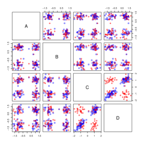
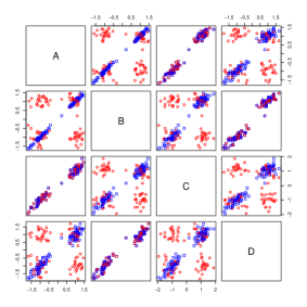
(a)	(b)	(c)

Figure 1: (a) Pairplot matrix of toy data. (b) Fully randomised data (red spheres) that models user’s knowledge and data where only relation between attributes $CD$ has been preserved (blue squares) that models what the user could learn of the relations between attributes $CD$. (c) As in (b), but additionally relation between attributes $AC$, as well as between attributes $BD$, has been preserved, modeling user’s knowledge of the relations between $AC$ and $BD$, respectively.

Our contribution consists of two main parts: (i) a framework to model and incorporate the user’s background knowledge of the data and to express the user’s objectives, and (ii) a system to show the most informative views of the data. The first contribution is general, but the second contribution, the most informative views of the data, is specific to a particular data type. In this paper we focus on data items that can be represented as real-valued vectors of attribute values.

As an example, consider the 4-dimensional toy data set shown in Fig. 1a. The dataset has been generated by first creating the strongly correlated attributes $A$ and $B$, and then generating attribute $C$ by adding noise to $A$, and attribute $D$ by adding noise to $B$. The purpose of this example is to show how the user’s background knowledge and objectives affect the views that are most informative to the user.

Assume the user is interested in the relation of attributes $C$ and $D$; we call the relation of interest a hypothesis. Our task is to find a maximally informative 1-dimensional projection of the data that takes both this objective and the user’s background knowledge into account.

First, assume that the user knows only the marginal distributions of the attributes but nothing of their relations. We argue that in such a case the user’s internal model of the data can be modeled by a distribution over data sets that we call the background distribution, which in this case can be sampled from by permuting the columns of the data matrix at random, shown by the red spheres in Fig. 1b. Because we are interested in the relation of $CD$ we create another distribution in which $CD$ are permuted together but the data is otherwise randomised, as shown by the blue squares in Fig. 1b. The red distribution models what the user knows and the blue what the user could optimally learn about the relation of $CD$ from the data. The red and blue distributions differ most in the plot $CD$—as one would expect!—and indeed the maximally informative 1-dimensional projection is given by $C+D$.

Secondly, assume that—unlike above—the user already knows the relationship of attributes $AC$ and $BD$, but does not yet know that attributes $AB$ are almost identical. We can repeat the previous exercise with the difference that we now add the user’s knowledge as constraints to both the red and blue distributions, i.e., we permute $AC$ and $BD$ together (modeling the user’s knowledge of these relations), as shown in Fig. 1c. Again, the red distribution models the user’s knowledge and the blue what the user could learn from the relation of $CD$ from the data, given that the user already knows the relationships of $AC$ and $BD$. The red and blue distributions differ most in plot $AB$ and therefore the user would gain most information if shown this view; indeed, the most informative projection is $A+B$. In other words, the knowledge of the relation of $A$ and $B$ gives maximal information about the relation of $CD$! This makes sense, because variables $CD$ are really connected via $AB$ through their generative process.

Background model and objectives. We model the user’s background knowledge by a distribution over all datasets. We define the distribution using permutations and constraints on the permutations, which we call tiles. A tile is defined by a subset of data items and attributes. All attributes within a tile are permuted with the same permutation to conserve the relation between attributes. When the user has not seen the data, we assume that the background distribution is unconstrained and can be sampled from by permuting each attribute of the data at random. The user can input observations of the data using tiles. Essentially, by constructing a tile the user acknowledges that he or she knows the relations within the tile.

The tiles can also be used to formalise the user’s objectives. For example, if the user is interested in the interaction between two groups of variables, he or she can define two distributions using tiles, which we call hypotheses: one in which the interaction of interest is preserved and one in which it is broken. Any difference between these two hypotheses gives the user new information about the interaction of interest.

Finding views. The data and the hypotheses are typically high-dimensional and it is in practice not possible to view all relations at once; if it were, the whole problem would be trivial by just showing the user the entire dataset in one view. As a consequence, we need to construct a visualisation or a dimensionality reduction method that shows the most informative view (defined in Sec. 2) of the differences between the hypotheses. We introduce a linear projection pursuit method that finds a projection in a direction in which the two hypotheses differ most. The proposed method seeks directions in which the ratio of the variance of these two distributions is maximal. At the limit of no background information and most generic hypotheses the method reduces to PCA (Thm. 2.4).

The domain of interactive data exploration sets some further requirements for any implementation. On one hand, our system has no need of scaling to a huge number of data points, since visualising an extremely large number of points makes no sense. In practice, if the number of data points is large enough, we can always downsample the data to a manageable size. Therefore, our system has essentially a constant time complexity with respect to the number of data items, but not to the number of attributes, as shown later in Sec. 3. On the other hand, the response times must be on the order of seconds for fluid interaction. This rules out many slow to compute but otherwise sound approaches.

In summary, the contributions of this paper are: (i) a computationally efficient formulation and implementation of the user’s background model and hypotheses using constrained randomisation, (ii) a dimensionality reduction method to show the most informative view to the user, and (iii) an experimental evaluation that supports that our approach is fast, robust, and produces easily understandable results. The Appendix contains an algorithm for merging tiles (Sec. A), and an example demonstrating exploration of the German data (Secs. B and C)

2 Methods

Let $X$ be an $n\times m$ data matrix (dataset). Here $X(i,j)$ denotes the $i$th element in column $j$. Each column $X(\cdot,j),\ j\in[m]$, is an attribute in the dataset, where we used the shorthand $[m]=\{1,\ldots,m\}$. Let $D$ be a finite set of domains (e.g., continuous or categorical) and let $D(j)$ denote the domain of $X(\cdot,j)$. Also let $X(i,j)\in D(j)\textrm{ for all }i\in[n],\ j\in[m]$, i.e., all elements in a column belong to the same domain, but different columns can have different domains. The derivation in Sec. 2.1 is generic, but in Sec. 2.3 we consider only real numbers, $D(j)\subseteq\mathbb{R}$ for all $j\in[m]$.

2.1 Background model and tile constraints

In this subsection, we introduce the permutation-based sampling method and tiles which can be used to constrain the sampled distribution and to express the user’s background knowledge and objectives (hypotheses). The sampled distribution is constructed so that in the absence of constraints (tiles) the marginal distributions of the attributes are preserved.

We define a permutation of the data matrix $X$ as follows.

Definition 2.1 (Permutation)

Let ${\mathcal{P}}$ denote the set of permutation functions of length $n$ such that
$\pi:[n]\mapsto[n]$ is a bijection for all $\pi\in{\mathcal{P}}$, and denote by $\left(\pi_{1},\ldots,\pi_{m}\right)\in{\mathcal{P}}^{m}$ the vector of column-specific permutations. A permutation $\widehat{X}$ of the data matrix $X$ is then given as $\widehat{X}(i,j)=X(\pi_{j}(i),j)$.

When permutation functions are sampled uniformly at random, we obtain a uniform sample from the distribution of datasets where each of the attributes has the same marginal distribution as the original data. We parametrise this distribution with tiles that preserve the relations in the data matrix $X$ for a subset of rows and columns: a tile is a tuple $t=(R,C)$, where $R\subseteq[n]$ and $C\subseteq[m]$. The tiles considered here are combinatorial (in contrast to geometric), meaning that rows and columns in the tile do not need to be consecutive. In an unconstrained case, there are $(n!)^{m}$ allowed vectors of permutations. The tiles constrain the set of allowed permutations as follows.

Definition 2.2 (Tile constraint)

Given a tile
$t=(R,C)$, the vector of permutations $\left(\pi_{1},\ldots,\pi_{m}\right)\in{\mathcal{P}}^{m}$ is allowed by $t$ iff the following condition is true for all $i\in[n]$, $j\in[m]$, and $j^{\prime}\in[m]$:

$$i\in R\wedge j,j^{\prime}\in C\\ \implies\pi_{j}(i)\in R\wedge\pi_{j}(i)=\pi_{j^{\prime}}(i).$$

Given a set of tiles $T$, a set of permutations is allowed iff it is allowed by all $t\in T$.

A tile defines a subset of rows and columns, and the rows in this subset are permuted by the same permutation function in each column in the tile. In other words, the relations between the columns inside the tile are preserved. Notice that the identity permutation is always an allowed permutation. Now, the sampling problem can be formulated as follows.

Problem 2.1 (Sampling problem)

Given a set of tiles $T$, draw samples uniformly at random from vectors of permutations in ${\mathcal{P}}^{m}$ allowed by $T$.

The sampling problem is trivial when the tiles are non-overlapping, since permutations can be done independently within each non-overlapping tile. However, in the case of overlapping tiles, multiple constraints can affect the permutation of the same subset of rows and columns and this issue must be resolved. To this end, we need to define the equivalence of two sets of tiles, which means that the same constraints are enforced on the permutations.

Definition 2.3 (Equivalence of sets of tiles)

Let $T$ and $T^{\prime}$ be two sets of tiles. $T$ is equivalent to $T^{\prime}$, if $P$ is allowed by $T$ iff $P$ is allowed by $T^{\prime}$ for all vectors of permutations $P\subseteq\mathcal{P}^{m}$.

We say that a set of tiles $\mathcal{T}$ where no tiles overlap, is a tiling. Next, we show that there always exists a tiling equivalent to a set of tiles.

Theorem 2.1

Given a set of (possibly overlapping) tiles $T$, there exists a tiling $\mathcal{T}$ that is equivalent to $T$.

• Let $t_{1}=(R_{1},C_{1})$ and $t_{2}=(R_{2},C_{2})$ be two overlapping tiles. Each tile describes a set of constraints on the allowed permutations of the rows in their respective column sets $C_{1}$ and $C_{2}$. A tiling $\{t^{\prime}_{1},t^{\prime}_{2},t^{\prime}_{3}\}$ equivalent to $\{t_{1},t_{2}\}$ is given by:

  $$\begin{array}[]{rcl}t^{\prime}_{1}&=&(R_{1}\setminus R_{2},C_{1}),\\ t^{\prime}_{2}&=&(R_{1}\cap R_{2},C_{1}\cup C_{2}),\\ t^{\prime}_{3}&=&(R_{2}\setminus R_{1},C_{2}).\end{array}$$

  Tiles $t^{\prime}_{1}$ and $t^{\prime}_{3}$ represent the non-overlapping parts of $t_{1}$ and $t_{2}$ and the permutation constraints by these parts can be directly met. Tile $t^{\prime}_{2}$ takes into account the combined effect of $t_{1}$ and $t_{2}$ on their intersecting row set, in which case the same permutation constraints must apply to the union of their column sets. It follows that these three tiles are non-overlapping and enforce the combined constraints of tiles $t_{1}$ and $t_{2}$. Hence, a tiling can be constructed by iteratively resolving overlap in a set of tiles until no tiles overlap. $\square$

Notice that merging overlapping tiles leads to wider (larger column set) and lower (smaller row set) tiles. The limiting case is a fully-constrained situation where each row is a separate tile and only the identity permutation is allowed. We provide an efficient algorithm for merging tiles in Appendix A.

2.2 Formulating hypotheses

Our goal is to compare two distributions and we constrain the distributions in question by forming hypotheses. Tilings are used to form the hypotheses. The so-called hypothesis tilings provide a flexible method for the user to specify the relations in which he or she is interested.

Definition 2.4 (Hypothesis tilings)

Given a subset of rows $R\subseteq[n]$, a subset of columns $C\subseteq[m]$, and a $k$-partition of the columns given by $C_{1},\ldots,C_{k}$, such that $C=\cup_{i=1}^{k}{C_{k}}$ and $C_{i}\cap C_{j}=\emptyset$ if $i\neq j$, a pair of hypothesis tilings is given by $\mathcal{T}_{H_{1}}=\{(R,C)\}$ and $\mathcal{T}_{H_{2}}=\cup_{i=1}^{k}{\{(R,C_{i})\}}$, respectively.

The hypothesis tilings define the items $R$ and attributes $C$ of interest and the relations between the attributes that the user is interested in (through the partition of $C$). Hypothesis 1 ($\mathcal{T}_{H_{1}}$) corresponds to a hypothesis where all relations in $(R,C)$ are preserved, and hypothesis 2 ($\mathcal{T}_{H_{2}}$) to a hypothesis where there are no unknown relations between attributes in the partitions $C_{1},\ldots,C_{k}$ of $C$.

For example, if the columns are partitioned into two groups $C_{1}$ and $C_{2}$ the user is interested in relations between the attributes in $C_{1}$ and $C_{2}$, but not in relations within $C_{1}$ or $C_{2}$. On the other hand, if the partition is full, i.e., $k=|C|$ and $|C_{i}|=1$ for all $i\in[k]$, then the user is interested in all relations between the attributes. In the latter case, the special case of $R=[n]$ and $C=[m]$ indeed reduces to unguided data exploration, where the user has no background knowledge and the hypothesis covers all inter-attribute relations in the data.

The user’s knowledge concerning relations in the data is described by tiles as well. As the user views the data she or he can highlight relations observed by tiles. For example, the user can mark an observed cluster structure with a tile involving the data points in the cluster and the relevant attributes. We denote the set of user-defined tiles by ${\mathcal{T}}_{u}$. In our general framework, the user compares two distributions characterised by the tilings $\mathcal{T}_{u}+\mathcal{T}_{H_{1}}$ and $\mathcal{T}_{u}+\mathcal{T}_{H_{2}}$, respectively. Here ‘$+$’ is used with a slight abuse of notation to denote the operation of merging tilings into an equivalent tiling. By $\mathcal{H}$ we denote the pair of hypotheses

(2.1) $$\mathcal{H}=\langle\mathcal{T}_{u}+\mathcal{T}_{H_{1}},\mathcal{T}_{u}+\mathcal{T}_{H_{2}}\rangle.$$

Note that $\mathcal{H}$ specifies two distributions over datasets, both parametrised by their respective tilings, from which we can draw samples as described in Sec. 2.1.

2.3 Finding views

We are now ready to formulate our second main problem, i.e., given two distributions characterised by the hypothesis pair $\mathcal{H}$, how can we find an informative view of the data maximally contrasting these two distributions. The answer to this question depends on the type of data and the visualisation selected. For example, the visualisations or measures of difference are different for categorical and real-valued data. The real-valued data discussed in this paper allows us to use projections (such as principal components) that mix attributes.

Problem 2.2 (Comparing hypotheses)

Given two distributions characterised by the pair $\mathcal{H}=\langle\mathcal{T}_{u}+\mathcal{T}_{H_{1}},\mathcal{T}_{u}+\mathcal{T}_{H_{2}}\rangle$, where $\mathcal{T}_{u}$ is a (user-defined) background model tiling, and $\mathcal{T}_{H_{1}}$ and $\mathcal{T}_{H_{2}}$ are hypothesis tilings, find the projection in which the distributions differ the most.

To formalise the optimisation criterion in Prob. 2.2, we define a gain function $G(u,\mathcal{H})$ by

(2.2) $$G(u,\mathcal{H})=u^{T}\Sigma_{1}u/u^{T}\Sigma_{2}u,$$

where $\Sigma_{1}$ and $\Sigma_{2}$ are the covariance matrices of the distributions parametrised by the tilings $\mathcal{T}_{u}+\mathcal{T}_{H_{1}}$ and $\mathcal{T}_{u}+\mathcal{T}_{H_{2}}$, respectively, and $u$ is the projection direction. The covariance matrices $\Sigma_{1}$ and $\Sigma_{2}$ can be found analytically by the following theorem.

Theorem 2.2

Given $j,j^{\prime}\in[m]$, the covariance of attributes $\mathrm{cov}(j,j^{\prime})$ under the distribution defined by the tiling $\mathcal{T}$ is given by $\mathrm{cov}(j,j^{\prime})=\sum\nolimits_{i=1}^{n}{a_{j}(i)a_{j^{\prime}}(i)}/n$, where

$$a_{l}(i)=\left\{\begin{array}[]{ll}Y(i,l),&i\in R_{j,j^{\prime}}\\ \sum\nolimits_{k\in R(i,l)}{Y(k,l)}/|R(i,l)|,&i\notin R_{j,j^{\prime}}\end{array}\right.$$

and $l\in\{j,j^{\prime}\}$. We denote by $R_{j,j^{\prime}}=\{i\in[n]\mid\exists(R,C)\in\mathcal{T}\ldotp i\in R\wedge j,j^{\prime}\in C\}$ the set of rows permuted together, by $Y(i,l)=X(i,l)-\sum\nolimits_{i=1}^{n}{X(i,l)}/n$ the centered data matrix, and by $R(i,l)\subseteq[n]$ a set satisfying $\exists C\subseteq[m]\ldotp(R(i,l),C)\in\mathcal{T}\wedge i\in R(i,l)\wedge l\in C$, i.e., the rows in a tile that data point $X(i,l)$ belongs to.

• The covariance is defined by

  $$\mathrm{cov}(j,j^{\prime})=E\left[\sum\nolimits_{i=1}^{n}{Y(\pi_{j}(i),j)Y(\pi_{j^{\prime}}(i),j^{\prime})}/n\right],$$

  where the expectation $E[\cdot]$ is defined over the permutations $\pi_{j}\in{\cal P}$ and $\pi_{j^{\prime}}\in{\cal P}$ of columns $j$ and $j^{\prime}$ allowed by the tiling, respectively. The part of the sum for rows permuted together $R_{j,j^{\prime}}$ reads

  $$\sum\nolimits_{i\in R_{j,j^{\prime}}}{E\left[Y(\pi_{j}(i),j)Y(\pi_{j^{\prime}}(i),j^{\prime})\right]}/n\\ =\sum\nolimits_{i\in R_{j,j^{\prime}}}{Y(i,j)Y(i,j^{\prime})}/n,$$

  where we have used $\pi_{j}(i)=\pi_{j^{\prime}}(i)$ and reordered the sum for $i\in R_{j,j^{\prime}}$. The remainder of the sum reads

  $$\sum\nolimits_{i\in R_{j,j^{\prime}}^{c}}{E\left[Y(\pi_{j}(i),j)Y(\pi_{j^{\prime}}(i),j^{\prime})\right]}/n\\ =\sum\nolimits_{i\in R_{j,j^{\prime}}^{c}}{E\left[Y(\pi_{j}(i),j)\right]E\left[Y(\pi_{j^{\prime}}(i),j^{\prime})\right]}/n,$$

  where $R_{j,j^{\prime}}^{c}=[n]\setminus R_{j,j^{\prime}}$ and the expectations have been taken independently, because the rows in $R_{j,j}^{c}$ are permuted independently at random. The result then follows from the observation that $E\left[Y(\pi_{l}(i),l)\right]=a_{l}(i)$ for any $i\in R_{j,j^{\prime}}^{c}$. $\square$

Now, the projection in which the distributions differ most is given by

(2.3) $$u_{\mathcal{H}}=\operatorname*{arg\,max}_{u\in\mathbb{R}^{m}}G(u,\mathcal{H}).$$

The vector $u_{\mathcal{H}}$ gives the direction in which the two distributions differ the most in terms of the variance. Here we could in principle use some other difference measure as well. We chose the form of Eq. (2.3) because it is intuitive and it can be implemented efficiently, as described in the following theorem.

Theorem 2.3

The solution to the optimisation problem of Eq. (2.3) is given by $u_{\mathcal{H}}=Wv$, where $v$ is the first principal component of $W^{T}\Sigma_{1}W$ and $W\in{\mathbb{R}}^{m\times m}$ is a whitening matrix [13] such that $W^{T}\Sigma_{2}W=I$.

• Using $u=Wv$ we can rewrite the gain of Eq. (2.2) as

  (2.4) $$G(Wv,\mathcal{H}) =v^{T}W^{T}\Sigma_{1}Wv/v^{T}W^{T}\Sigma_{2}Wv$$

  $$=v^{T}W^{T}\Sigma_{1}Wv/v^{T}v.$$

  Eq. (2.4) is maximised when $v$ is the maximal variance direction of $W^{T}\Sigma_{1}W$, from which it follows that the solution to the optimisation problem of Eq. (2.3) is given by $u_{\mathcal{H}}=Wv$, where $v$ is the first principal component of $W^{T}\Sigma_{1}W$. $\square$

In visualisations (when making two-dimensional scatterplots), we project the data to the first two principal components, instead of considering only the first component.

We note that at the limit of no background knowledge and with the most general hypotheses, our method reduces to the PCA of the correlation matrix, as shown by the following theorem.

Theorem 2.4

In the special case of the first step in unguided data exploration, i.e., comparing a pair of hypotheses specified by $\mathcal{H}=\langle\emptyset+\mathcal{T}_{H_{1}},\emptyset+\mathcal{T}_{H_{2}}\rangle$, where $\mathcal{T}_{H_{1}}=\{([n],[m])\}$ and $\mathcal{T}_{H_{2}}=\cup_{j=1}^{m}\{([n],\{j\})\}$, the solution to Eq. (2.3) is given by the first principal component of the correlation matrix of the data when the data has been scaled to unit variance.

• The proof follows from the observations that for $\mathcal{T}_{H_{2}}$ the covariance matrix $\Sigma_{2}$ is a diagonal matrix (here a unit matrix), resulting in the whitening matrix $W=I$. For this pair of hypotheses, $\Sigma_{1}$ denotes the covariance matrix of the original data. The result then follows from Thm. 2.3. $\square$

2.4 Selecting attributes for a tile constraint

Once we have defined the most informative projection, which displays the most prominent differences between the distributions parametrised by the pair of hypotheses, we can view the data in this projection. This allows the user to observe different patterns, e.g., a clustered set of points, a linear relationship or a set of outlier points.

After observing a pattern, the user defines a tile $(R,C)$ to be added to $\mathcal{T}_{u}$. The set of data points $R$ involved in the pattern can be easily selected from the projection shown. For selecting the attributes that characterise the pattern, we can use a procedure where for each attribute the ratio between the standard deviation of the attribute for the selection and the standard deviation of all data points is computed. If this ratio is below a threshold value $\tau$ (e.g., $\tau=0.5$), then the attribute is included in the set of attributes $C$ characterising the pattern. The intuition here is that we are looking for attributes in which the selection of points are more similar to each other than is expected based on the whole data.

3 Experiments

In this section we first consider the stability and scalability of the method presented in this paper. After this, we present two brief examples of how the method is used to (i) explore relations in a dataset and (ii) focus on investigating a hypothesis concerning relations in a subset of the data.

Dataset In the experiments, we utilise the german socio-economic dataset [1, 11]. The dataset contains records from 412 administrative districts in Germany. The full dataset has 46 attributes describing socio-economic, political and geographic aspects of the districts, but we only use 32 variables (see the Sections B and C in the Appendix for details) in the experiments. We scale the real-valued variables to zero mean and unit variance. All of the experiments were performed with a single-threaded R 3.5.0 [19] implementation on a MacBook Pro laptop with a 2.5 GHz Intel Core i7 processor.

3.1 Stability and scalability

We first study the sensitivity of the results with respect to noise or missing data rows. We begin the experiment by separating 32 real-valued variables and 3 (non-trivial) factors from the full german data. A synthetic dataset, parametrised by the noise term $\sigma$ and an integer $\Delta n$ is constructed as follows. First, we randomly remove $\Delta n$ rows, after which we to the remaining variables add Gaussian noise with variance $\sigma^{2}$, and finally rescale all variables to zero mean and unit variance. We create a random tile by randomly picking a factor that defines the rows in a tile and randomly pick 2–32 columns. The background distribution consists of three such random tiles and the hypothesis tiles are constructed of one such random tile $(R,C)$ as $\mathcal{T}_{H_{1}}=\{(R,C)\}$ and $\mathcal{T}_{H_{2}}=\cup_{j\in C}{\{(R,\{j\})\}}$.

$\sigma$	$\Delta n$	error
$0$	$0$	$0.000$
$0$	$200$	$0.038$
$1$	$0$	$0.088$
$1$	$200$	$0.135$
$10$	$0$	$0.562$
$10$	$200$	$0.664$

Table 1: The mean error as function of perturbance to data (noise with variance $\sigma$ added and $\Delta n$ random rows removed). The error is here the difference in gain of Eq. (2.2) between the optimal solution $u_{\mathcal{H}}$ to the solution $u_{\mathcal{H}}^{*}$ found on perturbed data.

$n$	$m$	$t_{\mathrm{model}}$ (s)	$t_{\mathrm{view}}$ (s)
$10^{3}$	$10$	$0.03$	$0.01$
$10^{4}$	$10$	$0.46$	$0.08$
$10^{3}$	$100$	$0.16$	$0.66$
$10^{4}$	$100$	$1.78$	$5.52$
$10^{3}$	$200$	$0.19$	$2.58$
$10^{4}$	$200$	$4.19$	$22.35$

Table 2: Median wall clock running time for random data with varying number of rows ($n$) and columns ($m$) for a dataset consisting of Gaussian random numbers. We give the time to add three random tiles plus hypothesis tiles ($t_{\mathrm{model}}$) and the time to find the most informative view ($t_{\mathrm{view}}$), i.e., to solve Eq. (2.3).

The results are shown in Tab. 1. We notice that the method is relatively insensitive with respect to the gain to noise and removal of rows. Even removing about half of the rows does not change the results meaningfully. Only very large noise, corresponding to $\sigma=10$ (i.e., c. 10% signal to noise ratio) degrades the results substantially.

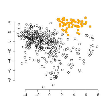
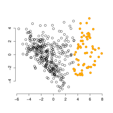
Figure 2: Views of the german dataset corresponding to the hypothesis pairs $\mathcal{H}_{E,\emptyset}$ (left) and $\mathcal{H}_{E,\{t\}}$ (right). Black circles ($\circ$) show data points; selected points are marked with orange.

Tab. 2 shows the running time of the algorithm as a function of the size of the data for Gaussian random data with a similar tiling setup as used for the german data. We make two observations. First, the tile operations scale linearly with the size of the data $nm$ and they are relatively fast. Most of the time is spent on finding the views, i.e., solving Eq. (2.3). Even our unoptimised pure R implementation runs in seconds for datasets that are visualisable (having thousands of rows and hundreds of attributes); any larger dataset should in any case be downsampled for visualisation purposes.

3.2 Human-guided data exploration of the german dataset

Finally, we demonstrate our human-guided data exploration framework by exploring the german dataset under different hypotheses. Sections B and C in the Appendix contain larger figures with more details (samples corresponding to both hypotheses and axes labelled with components of the projection vectors) and more thorough explanations of the exploration process described below.

We start with unguided data exploration where we have no prior knowledge about the data and our interest is as generic as possible. In this case $\mathcal{T}_{u}=\emptyset$ and as the hypothesis tilings we use $\mathcal{T}_{E_{1}}$, where all rows and columns belong to the same tile (a fully-constrained tiling), and $\mathcal{T}_{E_{2}}$, where all columns form a tile of their own (fully unconstrained tiling). Our hypothesis pair is then $\mathcal{H}_{E,\emptyset}=\langle\emptyset+\mathcal{T}_{E_{1}},\emptyset+\mathcal{T}_{E_{2}}\rangle$.

	$\mathcal{H}_{E,\emptyset}$	$\mathcal{H}_{E,\{t\}}$	$\mathcal{H}_{F,\emptyset}$	$\mathcal{H}_{F,\{t\}}$
$u_{E,\emptyset}$	8.831	3.887	1.921	1.124
$u_{E,\{t\}}$	7.933	8.920	1.172	1.100
$u_{F,\emptyset}$	4.879	2.062	2.958	1.087
$u_{F,\{t\}}$	1.618	1.842	1.489	1.773
$u_{\mathrm{pca}}$	8.831	3.887	1.921	1.124
$u_{\mathrm{ica}}$	0.004	0.004	1.000	0.999

Table 3: The value of the gain $G(u,\mathcal{H})$ for different projection vectors $u$ and hypothesis pairs $\mathcal{H}$.

Now, looking at the view where the distributions characterised by the pair $\mathcal{H}_{E,\emptyset}$ differ the most, shown in Fig. 2 (left), we observe cluster patterns. Selecting a set of data points allows us to investigate what kind of items and attributes the selected points represent. E.g., Cluster 1 (shown in orange in Fig. 2 (left)) corresponds to rural districts in Eastern Germany characterised by a high degree of voting for the Left party. We now add a tile constraint $t$ for the items in the observed pattern where the columns (attributes) are chosen as described in Sec. 2.4, using a threshold value $\tau=2/3$. The hypothesis pair is then updated to $\mathcal{H}_{E,\{t\}}=\langle\{t\}+\mathcal{T}_{E_{1}},\{t\}+\mathcal{T}_{E_{2}}\rangle$. The most informative view displaying differences of the distributions parametrised by $\mathcal{H}_{E,\{t\}}$ is now shown in Fig. 2 (right) and we observe that Cluster 2 (the selection shown in orange) has become prominent. By inspecting the class attributes of this selection we learn that these items correspond to urban districts.

Figure 3: Views of the german dataset corresponding to the hypothesis pairs $\mathcal{H}_{F,\emptyset}$ (left) and $\mathcal{H}_{F,\{t\}}$ (right). The circles $\circ$ show data points inside the focus area; the points outside the focus area are shown using $+$.

Next, we focus on a more specific hypothesis involving only a subset of rows and attributes. As the subset of rows $R$ we choose rural districts. As attributes of interest, we consider a partition $C=C_{1}\cup C_{2}\cup C_{3}\cup C_{4}$, where $C_{1}$ contains voting results for the political parties in 2009, $C_{2}$ contains demographic attributes, $C_{3}$ contains workforce attributes, and $C_{4}$ contains education, employment and income attributes. We here want to investigate relations between different attribute groups, ignoring the relations inside the groups.

We form the hypothesis pair $\mathcal{H}_{F,\emptyset}=\langle\emptyset+\mathcal{T}_{F_{1}},\emptyset+\mathcal{T}_{F_{2}}\rangle$, where $\mathcal{T}_{F_{1}}$ consists of a tile spanning all rows in $R$ and all columns in $C$ whereas $\mathcal{T}_{F_{2}}$ consists of four tiles: $t_{i}=(R,C_{i})$, $i\in\{1,2,3,4\}$. Looking at the view where the distributions parametrised by the pair $\mathcal{H}_{F,\emptyset}$ differ the most, shown in Fig. 3 (left), we find two clear clusters corresponding to a division of the districts into those located in the East, and those located elsewhere. We could also have used our already observed background knowledge of Cluster 1, by considering the hypothesis pair $\mathcal{H}_{F,\{t\}}=\langle\{t\}+\mathcal{T}_{F_{1}},\{t\}+\mathcal{T}_{F_{2}}\rangle$. For this hypothesis pair, the most informative view is shown in Fig. 3 (right), which clearly is different to Fig. 3 (left), demonstrating that the background knowledge is important.

To understand the utility of the views shown, we compute values of the gain function as follows. We consider our four hypothesis pairs $\mathcal{H}_{E,\emptyset}$, $\mathcal{H}_{E,\{t\}}$, $\mathcal{H}_{F,\emptyset}$, and $\mathcal{H}_{F,\{t\}}$. For each of these pairs, we denote the direction in which the two distributions differ most in terms of the variance (solutions to Eq. (2.3)) by $u_{E,\emptyset}$, $u_{E,\{t\}}$, $u_{F,\emptyset}$, and $u_{F,\{t\}}$, respectively. We then compute the gain $G(u,\mathcal{H})$ for each $u\in\{u_{E,\emptyset},u_{E,\{t\}},u_{F,\emptyset},u_{F,\{t\}}\}$ and $\mathcal{H}\in\{\mathcal{H}_{E,\emptyset},\mathcal{H}_{E,\{t\}},\mathcal{H}_{F,\emptyset},\mathcal{H}_{F,\{t\}}\}$. For comparison, we also compute the first PCA and ICA projection vectors, denoted by $u_{\mathrm{pca}}$ and $u_{\mathrm{ica}}$, respectively, and calculate the gain in different hypothesis pairs using these. The results are presented in Tab. 3. We notice that the gain is indeed always the highest when the projection vector matches the hypothesis pair (highlighted in the table), as expected. This shows that the views presented are indeed the most informative ones given the current background knowledge and the hypotheses being investigated. We also notice that the gain for PCA is equal to that of unguided data exploration, as expected by Thm. 2.4. When some background knowledge is used or if we investigate a particular hypothesis, the views achievable using PCA or ICA are less informative than using our framework. The gains close to zero for ICA are directions where the variance of the more constrained distribution is small due to, e.g., linear dependencies in the data.

4 Related work

Iterative data mining [9] is a paradigm where patterns already discovered by the user are taken into account as constraints during subsequent exploration. This concept of iterative pattern discovery is also central to the data mining framework presented in [4, 5, 6], where the user’s current knowledge (or beliefs) of the data is modelled as a probability distribution over datasets, and this distribution is then updated iteratively during the exploration phase as the user discovers new patterns. Our work has been motivated by [18, 16, 12, 17], where these concepts have been successfully applied in visual exploratory data analysis where the user is visually shown a view of the data which is maximally informative given the user’s current knowledge. Visual interactive exploration has also been applied in different contexts, e.g., in item-set mining and subgroup discovery [1, 8, 22, 15], information retrieval [20], and network analysis [2].

Solving the problem of determining which views of the data that are maximally informative to the user, and hence interesting, have been approached in terms of, e.g., different projections and measures of interestingness [7, 11, 23]. Constraints have also been used to assess the significance of data mining results, e.g., in pattern mining [14] or in investigating spatio-temporal relations [3].

The present work fundamentally differs from the above discussed previous work concerning iterative data mining and applications to visual exploratory data analysis in the following way. In previous work, the user is presented with informative views (visual or not) of the data, but the user cannot beforehand know which aspects of the data these views will show, since by definition the views are such that they contrast maximally with the user’s current knowledge. The implication is that the user cannot steer the exploration process. In the present work we solve this navigational problem by incorporating both the user’s knowledge of the data, and different hypotheses concerning the data into the background distribution.

5 Conclusions

In this paper we proposed a method to integrate both the user’s background model learned from the data and the user’s current interests in the explorative data analysis process. We provided an efficient implementation of this method using constrained randomisation. Furthermore, we extended PCA to work seamlessly with the framework in the case of real-valued datasets.

The power of human-guided data exploration stems from the fact that typical datasets contain a huge number of interesting patterns. However, the patterns that are interesting to a user depend on the task at hand. A non-interactive data mining method is therefore restricted to either show generic features of the data—which may already be obvious to an expert—or then output unusably many patterns (a typical problem, e.g., in frequent pattern mining: there are easily too many patterns for the user to absorb). Our framework is a solution to this problem: by integrating the human background knowledge and focus—formulated as a mathematically defined hypothesis—we can at the same time guide the search towards topics interesting to the user at any particular moment while taking the user’s prior knowledge into account in an understandable and efficient way.

This work could be extended, e.g., to understand classifier or regression functions in addition to static data and to different data types, such as time series. An interesting problem would also be to find an efficient algorithm that could find a sparse solution to the optimisation problem of Eq. (2.3). To our knowledge, no such solution is readily available as the solutions for sparse PCA are not directly applicable here; sparse PCA would give a sparse variant of the vector $v$ in Thm. 2.3, which would however not result in a sparse $u_{\mathcal{H}}=Wv$. An obvious next step would be to implement these ideas in interactive data analysis tools.

Appendix A Algorithm for merging tiles

Merging a new tile into a tiling where all tiles are non-overlapping can be done efficiently using Alg. 1. We assume that the starting point always is a non-overlapping set of tiles and hence we only need to consider the overlap that the new tile has with the tiles already existing in the tiling. This is similar to the merging of statements considered in [10].

The algorithm for merging tiles has two steps. Let $\mathcal{T}$ be the existing tiling (with non-overlapping tiles) and let $t=(R,C)$ be the new tile to be added to the tiling, where $R$ is the set of rows and $C$ is the set of columns spanned by the tile $t$. In the first step (lines 1–11) we identify those tiles in the tiling $\mathcal{T}$ with which $t$ overlaps. In the second step we resolve (merge) the overlap between $t$ and the tiles identified in $\mathcal{T}$. The algorithm proceeds as follows.

An empty hash map is initialised (line 1) in order to be used to detect overlap between columns of existing tiles in $\mathcal{T}$ and the new tile $t$. We proceed to iterate over each row $R$ in the new tile (lines 2–11).

The matrix $\mathcal{T}$ is of the same size as the data matrix and contains information on which tiles that cover a particular part of the data matrix. Each element in $\mathcal{T}$ hence holds information concerning which tile that occupies a particular region. Since the tiling described by $\mathcal{T}$ is non-overlapping, it means that each element in $\mathcal{T}$ corresponds to the ID of the tile that covers that position. Given a row $i\in R$ and a set of columns $C$ (line 3) we then get the IDs of the tiles on row $i$ with which $t$ overlaps and we store this in $K$. The hash map is used to detect if this row has been seen before, i.e., if $K$ is a key in $S$ (line 4). If this is the first time this row is seen, $K$ is used as the key for a new element in the hash map and $S(K)$ is initialised to be a tuple (line 5). Elements in this tuple are referred to by name, e.g., $S(K)_{\mathrm{rows}}$ gives the set of rows associated with the key $K$, while $S(K)_{\mathrm{id}}$ gives the set of tile IDs.

On lines 6 and 7 we store the current row index $S(K)_{\mathrm{rows}}$ and the unique tile IDs $S(K)_{\mathrm{id}}$ in the tuple. If the row was seen before, the row set associated with these tile IDs is updated (line 9). After this first step, the hash map $S$ contains tuples of the form (rows, id) where id specifies the IDs of the tiles with which $t$ overlaps at the rows specified by rows.

We then proceed to the second step in the algorithm (lines 12–16) where the identified overlap is resolved. We first determine the currently largest tile ID in use (line 12). After this we iterate over the tuples in the hash map $S$. For each tuple we must update the tiles having IDs $S(K)_{\mathrm{id}}$ and on line 14 we hence find the columns associated with these tiles. After this, the IDs of the affected overlapping tiles are updated (line 15), and the tile ID counter is incremented. Finally, the updated tiling is returned on line 17. The time complexity of the tile merging algorithm is $\mathcal{O}{(nm)}$.

input : (1) A tiling $\mathcal{T}$ ($n\times m$ data matrix where each element is the ID of the tile it belongs to)

(2) A new tile $t=(R,C)$.

output : $\mathcal{T}+\{t\}$ (the tiling $\mathcal{T}$ merged with $t$).

$S\leftarrow\texttt{HashMap}$;

for $i\in R$ do

       $K\leftarrow\mathcal{T}(i,C)$;

       if  $K\notin\texttt{keys}(S)$ then

             $S(K)\leftarrow\texttt{Tuple}$;

             $S(K)_{\mathrm{rows}}\leftarrow\{i\}$;

             $S(K)_{\textrm{id}}\leftarrow\texttt{unique}(\mathcal{T}(i,C))$;

            

       else

             $S(K)_{\textrm{rows}}\leftarrow S(K)_{\textrm{rows}}\cup\{i\}$;

            

       end if

      

end for

$p_{\mathrm{max}}\leftarrow\max(\mathcal{T}(R,C))$;

for $K\in\texttt{keys}(S)$ do

       $C^{\prime}=\left\{c\mid\mathcal{T}(S(K)_{\mathrm{rows}},c)\in S(K)_{\textrm{id}}\right\}$ ;

       $\mathcal{T}\left(S(K)_{\textrm{rows}},C^{\prime}\right)\leftarrow p_{\mathrm{max}}+1$;   $p_{\mathrm{max}}\leftarrow p_{\mathrm{max}}+1$;

      

end for

return $\mathcal{T}$

Algorithm 1 Merging a new tile $t$ with tiles in a tiling $\mathcal{T}$. The function HashMap denotes a hash map. The value in a hash map $H$ associated with a key $x$ is $H(x)$ and $\texttt{keys}(H)$ gives the keys of $H$. The function Tuple creates a (named) tuple. An element $a$ in a tuple $w=(\mathrm{a},\mathrm{b})$ is accessed as $w_{\mathrm{a}}$. The function unique returns the unique elements of an array.

Figure 4: Step 1 in the exploration of the dataset. The data points are shown by black spheres. Samples from the first part of the hypothesis pair are shown with green squares and samples from the second part with blue triangles. The selected cluster of points (see the text for discussion) is shown with orange colour. The axis labels show the five coefficients with the largest absolute values of each projection vector.

Appendix B Exploration of the German data without background knowledge

Dataset

In the experiments we consider the german socio-economic dataset [1, 11]. The dataset contains records from 412 administrative districts in Germany. Each district is represented by 46 attributes describing socio-economic and political aspects in addition to attributes such as the type of the district (rural/urban), area name/code, state, region and the geographic coordinates of each district center. The socio-ecologic attributes include, e.g., population density, age and education structure, economic indicators (e.g., GDP growth, unemployment, income), and the proportion of the workforce in different sectors. The political attributes include election results of the five major political parties (CDU/CSU, SPD, FDP, Green, and Left) in the German federal elections in 2005 and 2009, as well as the voter turnout. For our experiments we remove the election results from 2005, all non-numeric variables, and the area code and coordinates of the districts, resulting in 32 real-valued attributes (although we use the full dataset when interpreting the results). We scale the real-valued variables to zero mean and unit variance.

Step 1

We first consider the case where the data miner has no prior knowledge concerning the relations in the data, i.e., we have no initial background knowledge. We hence set $\mathcal{T}_{u}=\emptyset$ and as the hypothesis tilings we use $\mathcal{T}_{E_{1}}$, where all rows and columns belong to the same tile (a fully-constrained tiling), and $\mathcal{T}_{E_{2}}$, where all columns form their own tile (fully unconstrained tiling). Our hypothesis pair is then $\mathcal{H}_{E,\emptyset}=\langle\emptyset+\mathcal{T}_{E_{1}},\emptyset+\mathcal{T}_{E_{2}}\rangle$.

We then consider the first view of the data (Figure 4), which is maximally informative in terms of the two distributions parametrised by the hypotheses differing the most. In our figures we use black circles ($\circ$) to denote the real data points. We mark selected clusters with orange. Green squares ($\square$) denote points belonging to the data sample from the distribution parametrised by $\mathcal{T}_{u}+\mathcal{T}_{E_{1}}$ and blue triangles ($\triangle$) denote points belonging to the data sample from the distribution parametrised by $\mathcal{T}_{u}+\mathcal{T}_{E_{2}}$. Note that in this particular case the actual data and the sample corresponding to $\mathcal{T}_{u}+\mathcal{T}_{E_{1}}$ are identical (although the rows might be in different order), since this is a fully constrained tiling. The $x$ and $y$ axis labels show the five attributes with the largest absolute values of each projection vector.

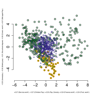
(a) Hypotheses updated with the knowledge concerning Cluster 1 (marked here for illustration purposes).

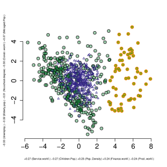
(b) Cluster 2 marked.

Figure 5: Step 2 in the exploration of the dataset. The meaning of the points is as in Fig. 4. Left: Hypotheses updated with the knowledge of Cluster 1 (marked here for illustration purposes). Right: Cluster 2 marked.

We observe that there are cluster patterns visible in the data and that the two distributions differ (the green and blue points are distributed differently). In order to investigate the characteristics of the data points, corresponding to different patterns in the german data, we select a set of points that form a cluster. Here we first choose to focus on the set of points in the upper right corner, marked with orange in Figure 4.

We now want to learn about the cluster we have identified. We consider the Type and Region attributes for the subset of data points (the marked cluster in the view) in the original data. These two categorical attributes tell whether a district in a cluster is urban or rural (Type) and where in Germany it is located (Region); in the Northern, Southern, Western, or Eastern region. For Cluster 1, we obtain the information shown in Table 4(a).

Region	Type
East :62	Rural:62
North: 0	Urban: 0
South: 0
West : 0

(a) Cluster 1.

Region	Type
East :22	Rural: 0
North:10	Urban:60
South: 7
West :21

(b) Cluster 2.

Table 4: Region and Type attributes for clusters observed in the data.

We also consider a parallel coordinates plot of the data, shown in Figure 6(a). This plot shows all 32 attributes in the data. The currently selected points (Cluster 1) are shown with red while the rest of the data is shown in black. The number in parentheses following each variable name is the ratio of the standard deviation of the selection and the standard deviation of all data. If this number is small we can conclude that the values for a particular attribute are homogeneous inside the selection (behave similarly).

Cluster 1 hence corresponds to Urban areas in the East. Based on the parallel coordinates plot in Figure 6(a), one clear political feature which we can observe is that there is little support for the Green party and a high support for the Left party in these districts.

Step 2

We continue our exploration by adding a tile constraint for Cluster 1. The set of rows for the tile is determined by our selection (marked in Figure 4). To determine the set of columns for the tile constraint we use the following heuristic: using the parallel coordinates plot (Figure 6(a)) we choose as columns for the tile those attributes for which the standard deviation ratio (the number in parentheses) $\tau$ is less than $2/3$.

We then update our hypotheses to take into account the newly added tile, i.e., consider the hypothesis pair $\mathcal{H}_{E,\{t\}}=\langle\{t\}+\mathcal{T}_{E_{1}},\{t\}+\mathcal{T}_{E_{2}}\rangle$. The most informative view is shown in Figure 5(a), We have here for illustration purposes marked Cluster 1 with orange. As can be seen, this cluster is no longer as clearly visible as in our first view in Figure 4. This is expected, since this pattern has been accounted for in the background distribution and the relations in this cluster no longer differ between the data samples corresponding to the distributions characterised by the hypothesis pair we are currently investigating. Instead we observe Cluster 2, marked in Figure 5(b). In a similar fashion as we did for Cluster 1, we consider the Region and Type attributes for Cluster 2 (Table 4(b)) and conclude that we have found urban districts spread out over all regions. Based on the parallel coordinates plot shown in Figure 6(b) we can conclude that these districts are characterised by a low fraction of agricultural workforce and a high amount of service workforce, both as expected in urban districts. We also notice that these districts have had a high GDP growth in 2009 and that it appears that the amount of votes for the CDU party in these districts was quite low.

(a) Parallel coordinates plot with Cluster 1 highlighted.

(b) Parallel coordinates plot with Cluster 2 highlighted.

Figure 6: Parallel coordinates plots of the two clusters. Left: Cluster 1 highlighted; right: Cluster 2 highlighted.

Group	Attributes
$C_{1}$	LEFT.2009, CDU.2009, SPD.2009,
	FDP.2009, GREEN.2009
$C_{2}$	Elderly.pop., Old.Pop., Mid.aged.Pop.,
	Young.Pop., Children.Pop.
$C_{3}$	Agricult..workf., Prod..workf.,
	Manufac..Workf., Constr..workf.,
	Service.workf., Trade.workf.,
	Finance.workf., Pub..serv..workf.
$C_{4}$	Highschool.degree, No.school.degree,
	Unemploy., Unempl..Youth, Income

Table 5: Column groups in the focus tile.

Appendix C Exploration of the german data with specific hypotheses

Case 1: No background knowledge

In this section we consider investigating hypotheses involving a subset of data items (rows in the data matrix, corresponding to different districts) and attributes.

We want to investigate a hypothesis concerning the relations between certain attribute groups in rural areas. We hence define our hypotheses as follows. As the subset of rows $R$ we choose all districts that are of the rural type. We then partition a subset of the attributes into four groups. The first attribute group ($C_{1}$) consists of the voting results for the political parties in 2009. The second attribute group ($C_{2}$) describes demographic properties such as the fraction of elderly people, old people, middle aged people, young people, and children in the population. The third group ($C_{3}$) contains attributes describing the workforce in terms of the fraction of the different professions such as agriculture, production, or service. The fourth group ($C_{4}$) contains attributes describing the education level, unemployment, and income. The attribute groupings are listed in Table 5.

(a) Cluster 3 marked

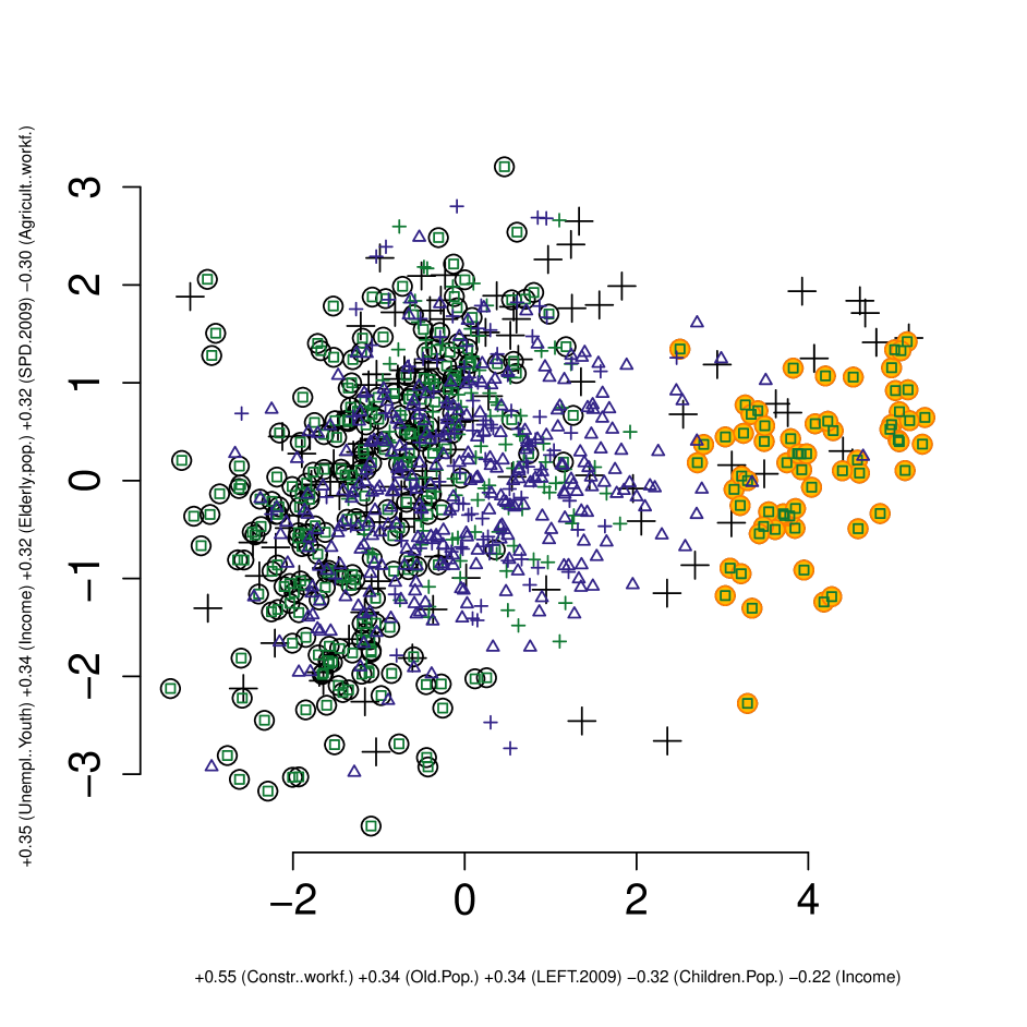
(b) Cluster 4 marked

(c) Parallel coordinates plot with Cluster 3 highlighted.

(d) Parallel coordinates plot with Cluster 4 highlighted.

Figure 7: Initial view of the data. Top row: symbols as in Fig. 4, except that points outside the focus area are shown using $+$ where black means data, and green and blue means samples from the first and second part of the hypothesis pair, respectively. Two visible clusters (3 and 4) are marked. Bottom row: parallel coordinates plots of the two clusters.

We then form a hypothesis pair $\mathcal{H}_{F,\emptyset}=\langle\emptyset+\mathcal{T}_{F_{1}},\emptyset+\mathcal{T}_{F_{2}}\rangle$, where $\mathcal{T}_{F_{1}}$ consists of a tile spanning all rows in $R$ and the columns $C=C_{1}\cup C_{2}\cup C_{3}\cup C_{4}$ whereas $\mathcal{T}_{F_{2}}$ consists of tiles $(R,C_{i})$, $i\in[4]$. These focus tiles allow us to investigate whether there are relations between these attribute groups, while ignoring relations inside the attribute groups.

The view where the distributions characterised by the pair $\mathcal{H}_{F,\emptyset}$ differ the most is shown in Figure 7(a). Again, we use green squares ($\square$) to denote items belonging to the data sample corresponding to $\mathcal{T}_{u}+\mathcal{T}_{F_{1}}$ and blue triangles ($\triangle$) to denote items belonging to the data sample corresponding to $\mathcal{T}_{u}+\mathcal{T}_{F_{2}}$. The points outside the focus area are shown using a plus-sign ($+$). We notice a clear division into two clusters, one on the left (marked in Figure 7(a)) and one on the right (marked in Figure 7(b)). We now investigate these two clusters in a similar fashion as we did before when exploring the relations in the data. Based on the Region and Type attributes for the clusters shown in Table 6, we conclude that Cluster 3 represents rural districts in the North, South and West, whereas Cluster 4 represents rural districts in the East. Based on the parallel coordinates plots in Figure 7(c) and Figure 7(d) it is clear that the voting behaviour is one aspect separating Cluster 3 and Cluster 4. In Cluster 4, the support for the Left party is prominent. Also, the fraction of old people in the population in Cluster 4 is larger, whereas the fraction of children in the population is high in Cluster 3. We conclude that there are interesting relations between the attribute groups considered, which means, e.g., that there is a connection between demographic properties and voting behaviour in the different rural districts.

Region	Type
East : 0	Rural:233
North: 48	Urban: 0
South:106
West : 79

(a) Cluster 3.

Region	Type
East :64	Rural:65
North: 0	Urban: 0
South: 0
West : 1

(b) Cluster 4.

Table 6: Region and Type attributes for clusters observed in the data when focusing on a subset.

Case 2: Using background knowledge

We could also have used our already observed background knowledge. Let $t$ be a tile corresponding to Cluster 1 in Table 4(a). We hence consider the hypothesis pair $\mathcal{H}_{F,\{t\}}=\langle\{t\}+\mathcal{T}_{F_{1}},\{t\}+\mathcal{T}_{F_{2}}\rangle$. Using these hypotheses we get the view shown in Figure 8. This view is clearly different than Figure 7(a), since we already were aware of the relations concerning the rural districts in the East and this was included in our background knowledge. We hence conclude that the background knowledge matters when comparing hypotheses.

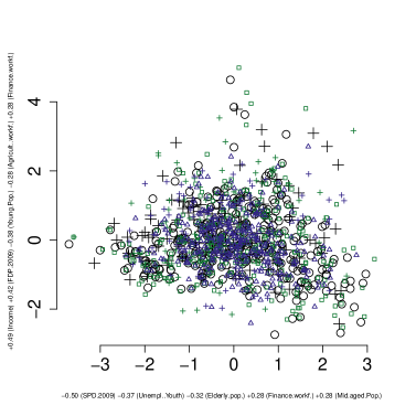
Figure 8: Initial view of the data using Cluster 1 (Tab. 4(a)) as background knowledge. Symbols as in Fig. 7(a).

References

- [1] M. Boley, M. Mampaey, B. Kang, P. Tokmakov, and S. Wrobel. One click mining—interactive local pattern discovery through implicit preference and performance learning. In KDD-IDEA, pages 27–35, 2013.
- [2] D. Chau, A. Kittur, J. Hong, and C. Faloutsos. Apolo: making sense of large network data by combining rich user interaction and machine learning. In CHI, pages 167–176, 2011.
- [3] F. Chirigati, H. Doraiswamy, T. Damoulas, and J. Freire. Data polygamy: the many-many relationships among urban spatio-temporal data sets. In SIGMOD/PODS, pages 1011–1025, 2016.
- [4] T. De Bie. An information theoretic framework for data mining. In KDD, pages 564–572, 2011.
- [5] T. De Bie. Maximum entropy models and subjective interestingness: an application to tiles in binary databases. Data Min. Knowl. Discov., 23(3):407–446, 2011.
- [6] T. De Bie. Subjective interestingness in exploratory data mining. In IDA, pages 19–31, 2013.
- [7] T. De Bie, J. Lijffijt, R. Santos-Rodriguez, and B. Kang. Informative data projections: a framework and two examples. In ESANN, pages 635 – 640, 2016.
- [8] V. Dzyuba and M. van Leeuwen. Interactive discovery of interesting subgroup sets. In IDA, pages 150–161, 2013.
- [9] S. Hanhijärvi, M. Ojala, N. Vuokko, K. Puolamäki, N. Tatti, and H. Mannila. Tell me something I don’t know: randomization strategies for iterative data mining. In KDD, pages 379–388, 2009.
- [10] J. Kalofolias, E. Galbrun, and P. Miettinen. From sets of good redescriptions to good sets of redescriptions. In ICDM, pages 211–220, 2016.
- [11] B. Kang, J. Lijffijt, R. Santos-Rodríguez, and T. De Bie. Subjectively interesting component analysis: Data projections that contrast with prior expectations. In KDD, pages 1615–1624, 2016.
- [12] B. Kang, K. Puolamäki, J. Lijffijt, and T. De Bie. A tool for subjective and interactive visual data exploration. In ECML-PKDD, pages 3–7, 2016.
- [13] A. Kessy, A. Lewin, and K. Strimmer. Optimal whitening and decorrelation. Am. Stat., 2018. Published online 26 Jan 2018.
- [14] J. Lijffijt, P. Papapetrou, and K. Puolamäki. A statistical significance testing approach to mining the most informative set of patterns. DMKD, 28(1):238–263, 2014.
- [15] D. Paurat, R. Garnett, and T. Gärtner. Interactive exploration of larger pattern collections: A case study on a cocktail dataset. In KDD-IDEA, pages 98–106, 2014.
- [16] K. Puolamäki, B. Kang, J. Lijffijt, and T. De Bie. Interactive visual data exploration with subjective feedback. In ECML-PKDD, pages 214–229, 2016.
- [17] K. Puolamäki, E. Oikarinen, B. Kang, J. Lijffijt, and T. D. Bie. Interactive visual data exploration with subjective feedback: An information-theoretic approach. In ICDE, pages 1208–1211, 2018.
- [18] K. Puolamäki, P. Papapetrou, and J. Lijffijt. Visually controllable data mining methods. In ICDMW, pages 409–417, 2010.
- [19] R Core Team. R: A Language and Environment for Statistical Computing. R Foundation for Statistical Computing, Vienna, Austria, 2018.
- [20] T. Ruotsalo, G. Jacucci, P. Myllymäki, , and S. Kaski. Interactive intent modeling: Information discovery beyond search. CACM, 58(1):86–92, 2015.
- [21] J. W. Tukey. Exploratory data analysis. Addison-Wesley, 1977.
- [22] M. van Leeuwen and L. Cardinaels. Viper—visual pattern explorer. In ECML-PKDD, pages 333–336, 2015.
- [23] M. Vartak, S. Rahman, S. Madden, A. Parameswaran, and N. Polyzotis. SeeDB: efficient data-driven visualization recommendations to support visual analytics. In PVLDB, volume 8(3), pages 2182–2193, 2015.