On physical scattering density fluctuations of amorphous samples

Abstract

Using some rigorous results by Wiener [(1930). Acta Math. 30, 118-242] on the Fourier integral of a bounded function and the condition that small-angle scattering intensities of amorphous samples are almost everywhere continuous, we obtain the conditions that must be obeyed by a function $\eta({\bf r})$ for this may be considered a physical scattering density fluctuation. It turns out that these conditions can be recast in the form that the $V\to\infty$ limit of the modulus of the Fourier transform of $\eta({\bf r})$, evaluated over a cubic box of volume $V$ and divided by $\sqrt{V}$, exists and that its square obeys the Porod invariant relation. Some examples of one-dimensional scattering density functions, obeying the aforesaid condition, are also numerically illustrated.

Synopsis: A function can be considered a physical scattering density fluctuation if the modulus of its Fourier transform, evaluated over a finite volume $V$ and divided by $\sqrt{V}$, tends to a bounded non-vanishing function as $V\to\infty$ and if the squared limit obeys the Porod invariant relation.

Keywords: small angle scattering intensity, scattering density fluctuation, generalized harmonic analysis

1. Introduction

In classical physics the scattering theory is based on the assumption that a sample is characterized by a scattering density function $n({\bf r})$ (Guinier, 1952; Guinier & Fournet, 1955, Feigin & Svergun, 1987), the existence of which is assumed without discussing its mathematical properties. The aim of this paper is to discuss this aspect.
Let us briefly recall the main equations that allow us to pass from the scattering density function to the scattering intensity. The main step is the fact that $dv$, the sample’s infinitesimal volume element set at the point ${\bf r}$, contributes to the scattering amplitude with $n({\bf r})e^{i{\bf q}\cdot{\bf r}}dv$ [the modulus $q$ of the scattering vector ${\bf q}$ being related to the scattering angle $\vartheta$ and the wavelength $\lambda$ of the ingoing beam radiation by the relation $q=(4\pi/\lambda)\sin(\vartheta/2)$]. The normalized scattering intensity $I_{V}({\bf q})$ is the square modulus of the total scattering amplitude divided by volume of the illuminated portion of the sample and the intensity of the ingoing beam. Hence, setting the last quantity equal to one, it is simply given by the expression

$$I_{V}({\bf q})=|{\tilde{n}}_{V}({\bf q})|^{2}/V,$$ (1)

where ${\tilde{n}}_{V}({\bf q})$, the Fourier transform (FT) of $n_{V}({\bf r})$, is defined as

$${\tilde{n}}_{V}({\bf q})\equiv\int_{R^{3}}n_{V}({\bf r})e^{i{\bf q}\cdot{\bf r}}{\rm d}v=\int_{V}n({\bf r})e^{i{\bf q}\cdot{\bf r}}{\rm d}v.$$ (2)

Here $V$ denotes either the sample’s illuminated spatial set [generically having a right parallelepipedic shape] or this set’s volume, depending on the context, and $R^{3}$ the full three-dimensional Euclidean space. Besides, $n_{V}({{\bf r}})$ is defined according to

$$n_{V}({{\bf r}})\equiv\begin{cases}n({\bf r}),&\text{if}\quad{\bf r}\in V;\\ 0,&\text{elsewhere}.\end{cases}$$ (3)

One experimentally finds that:
A) - once $V$ exceeds a few of $\rm{mm}^{3}$, $I_{V}({\bf q})$ no longer depends on $V$, and
B) - if the position of the sample is varied with respect to the ingoing beam, no change in the collected scattering intensity is observed.
To make the last point evident, one substitutes $V$ with $V_{O}$ in the three above equations to emphasize the fact the illuminated part of the sample depends on the position of its gravity center $O$ even though its volume remains equal to $V$. Then, on a mathematical ground, experimental results A and B imply the existence of $\lim_{V\to\infty}I_{V_{O}}({\bf q})$ and that this value does not depend on $O$, i.e.

$$I({\bf q})=\lim_{V\to\infty}I_{V_{O}}({\bf q})=\lim_{V\to\infty}|{\tilde{n}}_{V_{O}}({\bf q})|^{2}/V.$$ (4)

Quantity $I(q)$ is commonly referred to as the normalized scattering intensity. This quantity is not directly observable because the counter pixels have a finite size (instead of a vanishing one, as we assumed above). This property implies that each pixel (say the $i$th) subtends a solid angle $\Delta\Omega_{i}$. Consequently, the signal ${\cal I}_{i}$ collected by the $i$th pixel is an integrated intensity given by

$${{\cal I}}_{i}=\int_{\Delta\Omega_{i}}I({\bf q}({\hat{\omega}}))d{\hat{\omega}}$$ (5)

with ${\bf q}({\hat{\omega}})\equiv(2\pi/\lambda)({\hat{\omega}}-{\hat{\omega}}_{in})$, where ${\hat{\omega}}_{in}$ specifies the direction of the ingoing beam and ${\hat{\omega}}$ that of the unit vector going from the sample (now treated as a point-like object since its largest diameter is much smaller than the distance of the sample from the counter) to a point of the pixel. It is commonly assumed that $I({\bf q}({\hat{\omega}}))$ be equal to ${\cal I}_{i}/\Delta\Omega_{i}$ within the angular range $\Delta\Omega_{i}$.[Once more, depending on the context, $\Delta\Omega_{i}$ denotes the set or the size.] Then, the resulting $I({\bf q})$ has a histogram shape and presents discontinuity points of the first order. One can compare set $\{{\cal I}_{i}\}$ of the integrated intensity values collected with a counter to another set $\{{{\cal I}_{i}}^{\prime}\}$ collected either by the outset but slightly shifted counter, so as to have $\Delta\Omega_{i}^{\prime}\neq\Delta\Omega_{i}$, or by a different counter with a better angular resolution, so as to have $\Delta\Omega_{i}^{\prime}\subset\Delta\Omega_{i}$. In both cases one finds that the discontinuity points of $I({\bf q})$ and $I^{\prime}({\bf q})$ are different and this indicates that most of the discontinuities are not intrinsic to $I({\bf q})$. Moreover, the heights of the jumps show a different behavior depending on the analyzed material. In fact, for some materials one finds that the amplitudes are approximately the same in the first case (i.e.  $\Delta\Omega_{i}^{\prime}\neq\Delta\Omega_{i}$) and reduced by about a $\Delta\Omega_{i}^{\prime}/\Delta\Omega_{i}$ factor in the second. For other materials and mainly in the only second case, one observes that some jump heights remain approximately the same while the remaining ones are reduced by about the previous factor. This phenomenon is easily understood if $I({\bf q})$ is written as

$$I({\bf q})=I_{c}({\bf q})+\sum_{j}c_{j}\delta({\bf q}-{\bf q}_{j})$$ (6)

where $I_{c}({\bf q})$ is a function (with possible discontinuities of the only first kind), $\delta(\cdot)$ denotes the Dirac function and the $c_{j}$s and the ${\bf q}_{j}$s are a set of positive constants and a set of scattering vectors, respectively. From expression (6), it follows that if, say, the pixels $\Delta\Omega_{i}$ and $\Delta\Omega_{k}^{\prime}$ contain the ${\bf q}_{j}$ vector, then ${\cal I}_{i}\approx{\cal I}_{k}^{\prime}\approx c_{j}$. This explains why the jumps, related to ${\bf q}_{j}$, remain unaltered by the use of two different counters. The materials presenting the first kind of behavior, i.e. with no Dirac-like contributions, are amorphous while those presenting the second kind of behavior present a certain degree of crystallinity. In the following we shall confine ourselves to the theory of small angle scattering (SAS) from amorphous samples. Thus, on the basis of the above experimental results, it will be assumed that:
C) - the small angle scattering intensity, relevant to any amorphous sample, is a function almost everywhere continuous throughout the full $q$ range.
It must be stressed that the SAS range of the observable $q$s is much more limited since it goes from $10^{-5}$ till $1$Å^-1. If the last upper bound were increased by a factor $10^{2}$ or more, the physics would drastically change because quantum and particle production effects can no longer be forgotten. In other words, the notion of scattering amplitude physically will no longer apply in the above reported form (see, e.g., Ciccariello, 2005). But, mathematically, the consideration of the FT for infinitely large values of $q$ does still make sense, and the validity of C at large ${\bf q}$s will only be considered from the last point of view. Concerning the reported lower bound, its presence is dictated by the necessity of introducing a beam stop in the experimental apparatus. The related limitation on the observable $q$s can to a large extent be overcome. In fact, as discussed in detail by Guinier & Fournet (1955) and, more recently, by Ciccariello (2017), in the experimentally accessible angular range the scattering intensity can be expressed in terms of the so called scattering density fluctuation $\eta({\bf r})$ that is simply obtained by subtracting to $n({\bf r})$ the mean value of the last quantity [i.e.  $\eta({\bf r})\equiv[n({\bf r})-\langle n\rangle]$, see equation (10) below]. Once A is obeyed, the relation existing between $I_{V}({\bf q})$ and $\eta({\bf r})$ is identical to equation (1) in so far it reads

$$I_{V}({\bf q})=|{\tilde{\eta}}_{V}({\bf q})|^{2}/V$$ (7)

where ${\tilde{\eta}}_{V}({\bf q})$ and $\eta_{V}({\bf r})$ are defined as ${\tilde{n}}_{V}({\bf q})$ and $n_{V}({\bf r})$ in equations (2) and (3). Adopting definition (1) one would find that the right hand side (rhs) diverges as ${\bf q}\to 0$. By contrast, the ${\bf q}\to 0$ limit of the rhs of (7) is finite since it is related to the isothermal compressibility of the analyzed sample. Then, hereinafter, the adopted definition of scattering intensity will be given by equation (7) or, more precisely, by the $V\to\infty$ limit of (7). Besides, the $I({\bf q})$ values in the angular range behind the beam stop, by assumption, are obtained extrapolating toward the origin of reciprocal space the observed $I_{V}({\bf q})$s. In this way, the sense of assumption C, for what concerns the full ${\bf q}$ range, is fully clarified. Combining now assumption C with assumptions A and B, from (7) one physically concludes that the FT ${\tilde{\eta}}_{V}(q)$ must be such that the following limit

$$I({\bf q})\equiv\lim_{V\to\infty}\Big{|}\frac{{\tilde{\eta}}_{V}({\bf q})}{\sqrt{V}}\Big{|}^{2}$$ (8)

exists throughout the full ${\bf q}$ range so as to define a function that is almost everywhere (a.e.) continuous function. This relation implies that the scattering density fluctuation $\eta({\bf r})$ relevant to any amorphous sample is such that the modulus of its FT, evaluated over a cubic set of volume V, must diverge as $V^{1/2}$ as $V\to\infty$, because in this way only relation (8) can hold true. Clearly, condition (8) considerably restricts the class of functions eligible to be the scattering density fluctuation of an amorphous sample. For instance, any $\eta({\bf r})$ which is squared modulus integrable (i.e. an $L_{2}$) function is a trivial scattering density fluctuation because it yields a vanishing scattering intensity, since its FT exists [see, e.g., Chandrasekharan, (1980)] and, consequently, once it is divided by $V^{1/2}$, limit (8) vanishes. Another trivial one-dimensional example is the function $\eta(x)=\sin^{2}(x)/|x|^{1/2}$ [see eq. (40) of Ciccariello, 2017] that is not $L_{2}$. Its FT over the interval $[-L,\,L]$ is

$$\quad-\sqrt{\frac{\pi}{4Lq(q^{2}-4)}}\Biggl{[}\sqrt{q(q+2)}\,\,C\Bigl{(}\sqrt{\frac{2L(q-2)}{\pi}}\Bigr{)}-$$

$$2\sqrt{q^{2}-4}\,\,C\Bigl{(}\sqrt{\frac{2Lq)}{\pi}}\Bigr{)}+\sqrt{q(q-2)}\,\,C\Bigl{(}\sqrt{\frac{2L(q+2)}{\pi}}\Bigr{)}\Biggr{]}$$

where $C(\cdot)$ denotes the Fresnel cosine integral (see, e.g., section 8.25 of Gradshteyn & Ryzhik, 1980). Using the asymptotic expression of the last function one easily verifies that, in the $L\to\infty$ limit, the above expression vanishes if $q\neq 0$ and is equal to 1 if $q=0$. These examples and other unsuccesfull attempts made by the present authors indicate that it is not trivial to find $\eta({\bf r})$ examples that obey equation (8). The basic question is then: which are the properties of $\eta({\bf r})$ for conditions A-C to be fulfilled?
Since scattering density fluctuations result from statistical mechanics averages (see, e.g., Morita & Hiroike, 1961), they are expected to be bounded functions. [In this respect it is noted that point-like (and, therefore, unbounded) scattering densities are often considered (Guinier, 1952) in dealing with crystalline materials. This only is a mathematical idealization, indeed quite useful because all the spatial configurations of the scattering centers, compatible with a given scattering intensity, can, at least in principle, be determined by the associated algebraic approach (see, e.g., Cervellino & Ciccariello, 2001).] Besides, scattering density fluctuation are also expected to contain some randomness elements owing to their statistical origin. This condition is quite hard to be translated into a mathematical definition but it suggests that the definition of scattering density fluctuations must conform to mathematical rules that are in some way probabilistic.
This paper will focus on these aspects. Using some rigorous mathematical results derived by Wiener in two papers (1930) and (1932), hereinafter referred to as I and II, it will be shown that:
S₁- any function $\eta({\bf r})$ can be considered a scattering density fluctuation if it has vanishing mean value, its FT is such that the limit reported on the rhs of equation (8) exists and obeys to

$$\int_{R^{3}}I({\bf q})dv_{q}=(2\pi)^{3}\langle\eta^{2}\rangle,$$ (9)

where $dv_{q}$ denotes the infinitesimal volume of reciprocal space and $\langle\eta^{2}\rangle$ the mean value of the squared density fluctuation. The above relation is known as Porod’s (1951) invariant relation.
The plan of the paper, that, for simplicity, is confined to one dimensional samples, is as follows. Section 2 deals with the introduction of the scattering density fluctuation $\eta(x)$ and the definition and some general properties of the associated correlation functions $\gamma(x)$ and $\gamma_{L}(x)$, which respectively refer to the infinitely large sample and to the sample of size $2L$. Section 3 essentially reports the basic work of Wiener (1930) who showed how to rigorously define the integrated scattering intensity starting from a generalized Fourier integral of $\gamma(x)$. We show that it is possible to achieve a more detailed characterization of functions $\eta({\bf r})$ using assumption C. In particular, it turns out that the $\gamma(x)$ of any amorphous sample is a continuous and an $L_{2}$ summable function. Section 4 shows the equivalence of this analysis and statement S₁. Moreover, it also reports two examples of scattering density fluctuations of the Méring-Tchoubar (1968) kind that obey relation (8). Finally, section 5 draws the final conclusions.

2. Definition and properties of the correlation function

The scattering density fluctuation (SDF) $\eta(x)$, associated to a scattering density function $n(x)$, is simply obtained by subtrating to $n(x)$ the mean value ${\langle n\rangle}$ of $n(x)$ evaluated all over the space. Thus,

$$\eta(x)\equiv n(x)-{\langle n\rangle}$$ (10)

with

$${\langle n\rangle}\equiv\lim_{L\to\infty}\frac{1}{2L}\int_{-L}^{L}n(x)dx=\lim_{L\to\infty}\frac{1}{2L}\int_{-\infty}^{\infty}n_{L}(x)dx,$$ (11)

where, similarly to definition (3), $n_{L}(x)$ is equal to $n(x)$ if $|x|\leq L$ and to zero elsewhere. The ${\langle n\rangle}$ value generally is finite and different form zero. From (10) and (11) follows that $\langle\eta\rangle$, the mean value of $\eta(x)$, vanishes. As already anticipated, it is physically by no way restrictive to assume that:
a) $|\eta(x)|$ is a bounded function (i.e. $|\eta(x)|\leq B$ whatever $x$ with $B>0$), integrable in the Lebesgue sense, and
b) it has no limit as $x\to\pm\infty$ so that $\eta(x)$ is expected to irregularly oscillate around zero.
One should note that the last condition, on the one hand, excludes that $\eta(x)$ may be an $L_{2}$ function and, on the other hand, it introduces some sort of randomness through the irregularity of the oscillations. Assumption a) ensures the validity of the following property:
P.1 - the mean value definition is translational invariant.
In fact, the mean value evaluated over the interval $[-L,\,L]$, translated by $a$, reads

$$\frac{1}{2L}\int_{-L+a}^{L+a}\eta(x)dx=\frac{1}{2L}\int_{-L-a}^{L+a}\eta(x)dx-\frac{1}{2L}\int_{-L-a}^{-L+a}\eta(x)dx.$$ (12)

Observing that

$$\frac{1}{2L}\int_{-L-a}^{L+a}\eta(x)dx=\frac{2(L+a)}{2L}\frac{1}{2(L+a)}\int_{-L-a}^{L+a}\eta(x)dx$$ (13)

and that

$$\Bigl{|}\frac{1}{2L}\int_{-L-a}^{-L+a}\eta(x)dx\Big{|}\leq\frac{1}{2L}\int_{-L-a}^{-L+a}|\eta(x)|dx\leq\frac{aB}{L},$$ (14)

one concludes that, whatever $a$,

$$\lim_{L\to\infty}\Bigl{[}\frac{1}{2L}\int_{-L-a}^{L+a}\eta(x)dx\Bigr{]}=\lim_{L\to\infty}\Bigl{[}\frac{1}{2L}\int_{-L}^{L}\eta(x)dx\Bigr{]}={\langle\eta\rangle}=0.$$ (15)

This result mathematically formulates the physical property that the mean value of a quantity, relevant to a macroscopically homogeneous material, is independent of the sampling, provided the sampled volume be sufficiently large.
The correlation function of a bounded sample, with SDF $\eta(x)$ and size $2L$, is defined as

$$\gamma_{L}(x)\equiv\frac{1}{2L}\int_{-\infty}^{\infty}\eta_{L}(x+y){\overline{\eta_{L}}}(y)dy=\frac{1}{2L}\int_{-L}^{L}\eta_{L}(x+y){\overline{\eta_{L}}}(y)dy.$$ (16)

where the overbar denotes the complex conjugate and $\eta_{L}(\cdot)$ is function $\eta(\cdot)$ restricted to the interval $[-L,\,L]$. This definition, due to Wiener (1930), generalizes the one adopted in SAS theory generally dealing with real $\eta(x)$s. It is also noted that one migth adopt the alternative definition

$$\Gamma_{L}(x)\equiv\frac{1}{2L}\int_{-L}^{L}\eta(x+y){\overline{\eta}}(y)dy.$$ (17)

If the SDF obeys condition a), the two definitions coincide in the limit $L\to\infty$, i.e.

$$\lim_{L\to\infty}\Gamma_{L}(x)=\lim_{L\to\infty}\gamma_{L}(x).$$ (18)

In fact, one finds that

$$\Gamma_{L}(x)-\gamma_{L}(x)=\frac{1}{2L}\int_{L-x}^{L}\eta(x+y){\overline{\eta(y)}}dy,\quad{\rm if}\quad x>0,$$ (19)

and, since

$$\Big{|}\frac{1}{2L}\int_{L-x}^{L}\eta(x+y){\overline{\eta(y)}}dy\Big{|}\leq\frac{1}{2L}\int_{L-x}^{L}B^{2}dy=\frac{x}{2L},$$ (20)

one immediately realizes that relation (18) is true because the case $x<0$ can similarly be handled. For brevity, the functions $\gamma_{L}(x)$ and $\Gamma_{L}(x)$ will be named limited correlation functions (LCF) to distinguish them from the correlation function (CF) relevant to the infinitely large sample. This is defined according to

$$\gamma(x)=\lim_{L\to\infty}\gamma_{L}(x)=\lim_{L\to\infty}\Gamma_{L}(x).$$ (21)

It will hereinafter be assumed that $\gamma(x)$ exists for any real $x$ value. It is also true the property that:
P.2 - The definition of LCF becomes translational invariant in the $L\to\infty$ limit.
In fact, if $a>0$, the difference between the translated and the outset definition of $\Gamma_{L}$ yields

$$\Big{|}\frac{1}{2L}\int_{-L+a}^{L+a}\eta(x+y){\overline{\eta}}(y)dy-\frac{1}{2L}\int_{-L}^{L}\eta(x+y){\overline{\eta}}(y)dy\Big{|}=$$

$$\frac{1}{2L}\Big{|}\int_{L}^{L+a}\eta(x+y){\overline{\eta}}(y)dy-\int_{-L}^{-L+a}\eta(x+y){\overline{\eta}}(y)dy\Big{|}\leq$$

$$\frac{1}{2L}\Bigl{[}\int_{L}^{L+a}B^{2}dy+\int_{-L}^{-L+a}B^{2}dy\Bigr{]}=\frac{aB^{2}}{L}.$$

The rightmost value tends to zero as $L\to\infty$ and the invariance is proved because the discussion of the case $a<0$ is quite similar.
The assumed boundedness of the SDF ensures that $\gamma_{L}(x)$ exists, is continuous everywhere and only differs from zero within the interval $[-2L,\,2L]$. However, the continuity property does not generally apply to $\gamma(x)$. An example, due to Wiener (II, pag. 151), makes this point evident. Assume that $\eta(x)=e^{ix^{2}}$ so as to obey condition a). One finds that

$$\Gamma_{L}(x)=\frac{1}{2L}\int_{-L}^{L}e^{i[(x+y)^{2}-y^{2}]}dy=\frac{e^{ix^{2}}}{2L}\int_{-L}^{L}e^{2ixy}dy$$

The last integral is equal to $2L$ if $x=0$ and to $\sin(2xL)/x$ if $x\neq 0$. Hence, in the $L\to\infty$ limit, one gets: $\gamma(x)=1$ if $x=0$ and $\gamma(x)=0$ if $x\neq 0$ and the CF is not continuous. This example shows that if one requires that $\gamma(x)$ exists, the class of the $\eta(x)$ functions must obey appropriate mathematical constraints. In fact, the condition that $\eta(x)$ is Lebesgue summable over any compact domain and everywhere bounded only is a sufficient condition. It is not easy to work out these constraints. They are implicitly defined assuming that:
P.3 - the $\eta(x)$ functions that can be SDFs belong to the set of functions that yield CFs that are defined throughout $(-\infty,\,\infty)$.
This set of functions will be denoted by ${\cal W}$ (in honor of Wiener who instead used symbol $S$.). We note now that:
P.4 - The function set ${\cal W}$ is a vectorial space.
To prove this property one has to show that: 1) if $\eta(x)\in{\cal W}$ then $\alpha\eta(x)\in{\cal W}$ for any complex number $\alpha$, and 2) if $\eta_{1}(x)$ and $\eta_{2}(x)\in{\cal W}$ then $[\eta_{1}(x)+\eta_{2}(x)]\in{\cal W}$. The first condition is obviously true. The proof of the second will slightly be postponed after we have reported two important theorems of Wiener (see II, pag. 154-156). The first states an important property, given for granted without any proof in SAS textbooks (Guinier & Fournet, 1955; Feigin & Svergun, 1987), i.e.:
P.5 - if $\eta(x)\in{\cal W}$, the correlation CF whatever $x$ obeys the inequality

$$|\gamma(x)|\leq\gamma(0)=\langle|\eta|^{2}\rangle,$$ (22)

where the rightmost equality follows from defintion (21) since $\langle|\eta|^{2}\rangle$ denotes the mean of the squared SDF. The second that:
P.6 - the correlation CF is everywhere continuous if it is continuous at $x=0$.
The proof of P.5 is somewhat simpler than that of Wiener (II, pag. 154) if, in agreement with a), one confines himself to ${{\cal W}_{b}}$, i.e.  the subset of the bounded functions belonging to ${\cal W}$. In fact, from definition (16), by the Schwarz inequality one gets

$$|\gamma_{L}(x)|^{2} = \Big{|}\frac{1}{2L}\int_{-L}^{L}\eta_{L}(x+y){\overline{\eta_{L}(y)}}dy\Big{|}^{2}\leq$$ (23)

$$\Big{[}\frac{1}{2L}\int_{-L}^{L}|\eta_{L}(x+y)|^{2}dy\Big{]}\Big{[}\frac{1}{2L}\int_{-L}^{L}|\eta_{L}(y)|^{2}dy\Big{]}.$$ (24)

One also has

$$\int_{-L}^{L}|\eta_{L}^{2}(x+y)|dy\leq\int_{-L}^{L}|\eta^{2}(x+y)|dy=\int_{-L+x}^{L+x}|\eta^{2}(t)|dt=$$

$$\int_{-L-x}^{L+x}|\eta^{2}(t)|dt-\int_{-L-x}^{-L+x}|\eta^{2}(t)|dt\leq\int_{-L-x}^{L+x}|\eta^{2}(t)|dt+\int_{-L-x}^{-L+x}|\eta^{2}(t)|dt\leq$$

$$\quad\quad\quad\int_{-L-x}^{L+x}|\eta^{2}(t)|dt+2xB^{2},$$ (25)

where, in obtaining the last relation, we used the fact that $|\eta(x)|\leq B$. After substituting the above inequality in equation (23) one gets

$$|\gamma_{L}(x)|^{2}\leq\Big{[}\frac{1}{2L}\int_{-L}^{L}|\eta_{L}^{2}(y)|dy\Big{]}\times$$

$$\Big{\{}\frac{2(L+x)}{2L}\Big{[}\frac{1}{2(L+x)}\int_{-(L+x)}^{L+x}|\eta^{2}(y)|dy\Big{]}+\frac{xB^{2}}{L}\Big{\}}.$$ (26)

In the $L\to\infty$ limit, the quantities inside the square brackets approach to $\gamma(0)$ while $xB^{2}/L$ and $2(L+x)/2L$ tend to zero and one, respectively. In this way P.5 is proved. To prove P.6, one starts from

$$|\gamma(x+\epsilon)-\gamma(x)|^{2}=\lim_{L\to\infty}\Big{|}\frac{1}{2L}\int_{-L}^{L}[\eta(x+\epsilon+t)-\eta(x+t)]{\overline{\eta}}(t)dt\Big{|}^{2}.$$ (27)

The above rhs (leaving momentarily aside the limit), by Schwartz’ inequality, does not exceed the quantity

$$\Bigl{[}\frac{1}{2L}\int_{-L}^{L}|\eta(x+\epsilon+t)-\eta(x+t)|^{2}dt\Bigr{]}\Bigl{[}\frac{1}{2L}\int_{-L}^{L}|\eta|^{2}(t)dt\Bigr{]}.$$ (28)

Expanding the integrand of the first integral, one gets four addends: $|\eta(x+\epsilon+t)|^{2}$, $|\eta(x+t)|^{2}$, $-\eta(x+\epsilon+t){\overline{\eta(x+t)}}$ and $-{\overline{\eta(x+\epsilon+t)}}\eta(x+t)$. The integration of each of these terms over $[-L,\,L]$, the subsequent limit $L\to\infty$ and the established translational invariance property respectively yield: $\gamma(0)$, $\gamma(0)$, $-\gamma(\epsilon)$ and $-{\overline{\gamma(\epsilon)}}$. Substituting these findings in the rhs of (27) one obtains

$$|\gamma(x+\epsilon)-\gamma(x)|^{2}\leq\bigl{[}2\gamma(0)-\gamma(\epsilon)-{\overline{\gamma(\epsilon)}}\bigr{]}\gamma(0),$$ (29)

which proves the theorem.
We complete now the proof that ${{\cal W}_{b}}$ is a vectorial space by showing that condition 2 also is obeyed. To this aim one must show that the $L\to\infty$ limit of

$$\frac{1}{2L}\int_{-L}^{L}[\eta_{1}(x+t)+\eta_{2}(x+t)]\overline{[[\eta_{1}(t)+\eta_{2}(t)]}dt$$ (30)

exists if $\eta_{1}$ and $\eta_{2}$ belong to ${{\cal W}_{b}}$. As it was done in equation (28), expanding the integrand one finds the LCFs $\Gamma_{1;L}(x)$ and $\Gamma_{2;L}(x)$, relevant to the SDFs $\eta_{1}(x)$ and $\eta_{2}(x)$, the integral

$$\Gamma_{1,2;L}(x)\equiv\frac{1}{2L}\int_{-L}^{L}\eta_{1}(x+t)\overline{\eta_{2}(t)}dt$$ (31)

and the integral $\Gamma_{2,1;L}(x)$. Since $\eta_{1}$ and $\eta_{2}$ belong to ${{\cal W}_{b}}$, the $L\to\infty$ limits of $\Gamma_{1,L}(x)$ and $\Gamma_{2,L}(x)$ will yield the CFs $\gamma_{1}(x)$ and $\gamma_{2}(x)$. By Schwartz’ inequality and the procedure followed to prove P.2, in the $L\to\infty$ limit one gets

$$|\Gamma_{1,2;L}(x)|\to|\gamma_{1,2}(x)|\leq\sqrt{\gamma_{1}(0)\,\gamma_{2}(0)}$$ (32)

and an identical relation for $|\Gamma_{2,1;L}(x)|$. In this way the proof of condition 2 is accomplished. Thus, ${{\cal W}_{b}}$ is a vectorial space and in the same way one proves that ${\cal W}$ also is a vectorial space.
We report some examples of SDFs which yield algebraically known CFs (II, pag. 151):
1 - if $\eta(x)\in L_{2}(-\infty,\infty)$, the associated CF identically vanishes. In fact, from the hypothesis follows that $\lim_{L\to\infty}\int_{-L}^{L}|\eta(x)|^{2}dx=\int_{-\infty}^{\infty}|\eta(x)|^{2}dx<\infty$. Then, $\gamma(0)=0$ by (21) and $\gamma(x)\equiv 0$ by (22);
2 - with the choice $\eta(x)=e^{i\alpha x}$ (with $\alpha\in R$), which is a bounded function with mean value equal to zero if $\alpha\neq 0$ and to one if $\alpha=0$, by equations (21) and (17) one finds that the associated CF again is $e^{i\alpha x}$ which is continuous throughout $R$;
3 - with the choice $\eta(x)=e^{i\alpha|x|^{a}}$ (with $\alpha$ real and $0<a<1$), generalizing the method reported at page 151 of II, the resulting CF turns out to be identically equal to 1;
4 - we already saw that the choice $\eta(x)=e^{i\alpha x^{2}}$ (with $\alpha$ real) yields: $\gamma(x)=1$ if $x=0$ and $\gamma(x)=0$ if $x\neq 0$, and the CF is now discontinuous by contrast to the previous cases.
Examples 1, 3 and 4 show that the problem: ”which is the function $\eta(x)$ which yields an assigned CF? or, equivalently, which is the $\eta(x)$ solution of the non linear integral equation

$$\lim_{L\to\infty}\frac{1}{2L}\int_{-L}^{L}\eta(x+y){\overline{\eta(y)}}dy=\gamma(x)$$ (33)

has an infinity of solutions. This conclusion is further strengthned by the property:
P.7 - if $\eta(x)$ is a solution of equation (33), any function of the kind $[\eta(x+a)+\eta_{1}(x)]$, with $a\in R$ and $\eta_{1}(x)\in L_{2}(-\infty,\,\infty)$, is solution of the same equation.
In fact, the proof that, for any real $a$, $\eta(x+a)$ reproduces the same CF of $\eta(x)$ is a consequence of P.2. If $\eta_{1}(x)\in L_{2}(-\infty,\,\infty)$, the proof that the function $\eta(x)+\eta_{1}(x)$ has the same CF of $\eta(x)$ immediately follows from example 1 and inequality (32). Finally, the linearity of ${\cal W}$ ensures that the property holds also true for $[\eta(x+a)+\eta_{1}(x)]$.

3. Wiener’s results on the SDF and CF Fourier integrals

We describe now the procedure followed by Wiener to rigorously evaluate the integrated scattering intensity. Some of his results, once combined with assumption C, are quite important for the theory of SAS from amorphous samples. Having confined ourselves to one-dimensional samples, equation (4) takes now the form

$$I(q)=\lim_{L\to\infty}I_{L}(q)=\lim_{L\to\infty}|{\tilde{\eta}}_{L}(q)|^{2}/2L,$$ (34)

where ${\tilde{\eta}}_{L}(q)$ denotes the FT of the SDF $\eta(x)$ evaluated over the interval $[-L,\,L]$. According to assumption a), $\eta_{L}(x)$, having the interval $[-L,\,L]$ as support, is a bounded $L_{1}(-L,\,L)$ function. Then, its Fourier transform

$${\tilde{\eta}}_{L}(q)\equiv\int_{-\infty}^{\infty}\eta_{L}(x)e^{iqx}dx$$ (35)

exists and is continuous for any $q$ value [see, e.g., Chandrasekharan (1989), pag. 2]. However, the limit $\lim_{L\to\infty}{\tilde{\eta}}_{L}(q)$ does not generally exist, because $\eta(x)$ does not approach zero at $x=\pm\infty$ and, therefore, it belongs neither to $L_{1}(-\infty,\,\infty)$ nor to $L_{2}(-\infty,\,\infty)$. The non existence of $\lim_{L\to\infty}{\tilde{\eta}}_{L}(q)$ is essential for equation (34) to make sense otherwise, if it would exist, one would find a vanishing scattering intensity.
This difficulty also applies to the FT of the CF generated by $\eta(x)$. In fact, equation(34) can be written, by definition (16), as

$$I(q)=\lim_{L\to\infty}\frac{1}{2L}\int_{-\infty}^{\infty}\int_{-\infty}^{\infty}\eta_{L}(x){\overline{\eta_{L}(y)}}e^{iq(x-y)}dxdy=$$

$$\quad\quad\quad\lim_{L\to\infty}\int_{-\infty}^{\infty}e^{iqt}\gamma_{L}(t).$$ (36)

According to P.5, so far it is only known that $\gamma(x)$ is bounded if $\eta(x)\in{{\cal W}_{b}}$, and this condition is not sufficient to ensure the existence of the rightmost limit present in (3. Wiener’s results on the SDF and CF Fourier integrals). Wiener (I, pag. 134) overcame the difficulty of the non existence of the above limit as well as of the $L\to\infty$ limit of ${\tilde{\eta}}_{L}(q)$ (I, pag. 151) introducing a factor of convergence within the relevant integrals. In fact, instead of ${\tilde{\eta}}_{L}(q)$, Wiener (II, pag. 138) considered function $s_{L}(q)$ defined as

$$s_{L}(q) \equiv s_{L,1}(q)+s_{2}(q)$$ (37)

with

$$s_{1,L}(q) \equiv \int_{1}^{\infty}\eta_{L}(x)\frac{e^{iqx}}{ix}dx+\int_{-\infty}^{-1}\eta_{L}(x)\frac{e^{iqx}}{ix}dx,$$ (38)

$$s_{2}(q) \equiv \int_{-1}^{1}\eta(x)\frac{e^{iqx}-1}{ix}dx.$$ (39)

[Omitting the factor $(2\pi)^{-1/2}$ we have slightly changed Wiener’s definition.] In (38) the integration bounds $\pm\infty$ can be set equal to $\pm L$. As far as $L$ is finite, functions $s_{L,1}(q)$ and $s_{2}(q)$ are entire functions of $q$ in the whole complex $q$ plane and one has

$$s^{\prime}_{L}(q)={\tilde{\eta}}_{L}(q),$$ (40)

where the prime denotes the derivative. It is noted that equations (38) and (39) can be combined into the form of a FT, i.e.

$$s_{L}(q+\epsilon)-s_{L}(q-\epsilon)=\int_{-\infty}^{\infty}\eta_{L}(x)\frac{2\sin(\epsilon x)}{x}e^{iqx}dx,$$ (41)

$\epsilon$ being a real number. Thus, $[s_{L}(q+\epsilon)-s_{L}(q-\epsilon)]$ is the FT of the $L_{1}[-L,\,L]$ function $2\eta_{L}(x){2\sin(\epsilon x)}/{x}$. The above equation can be inverted to get

$$\eta_{L}(x)=\frac{x}{4\pi\sin(\epsilon x)}\int_{-\infty}^{\infty}[s_{L}(q+\epsilon)-s_{L}(q-\epsilon)]e^{-iqx}dq.$$ (42)

The $L\to\infty$ limit is the crucial point because the corresponding limit of ${\tilde{\eta}}_{L}(q)$ generally does not exist since $\eta(x)$ neither belongs to $L_{1}$ nor to $L_{2}$. Actually, using the boundedness of $\eta(x)$ [i.e.  $|\eta(x)|\leq B$], from equation (41) one would get by theorem 1.5 of Chandrasekhar (1980) that the least upper bound, with respect to $L$, of $[s_{L}(q+\epsilon)-s_{L}(q-\epsilon)]$ cannot exceed $4B\log L$ (a bound diverging with $L$), as $q$ ranges over $R$. In reality, the last function is bounded and decreases at large $q$s. In fact, the presence of the factor $x$ in the integrands’ denominators of (38) ensures that $\eta_{L}(x)/x$ belongs to $L_{2}$ also in the $L\to\infty$ limit. Consequently, the integrals present in (38) exist and converge in the mean (a condition specified hereinafter by the symbol ”$\operatorname*{\rm{l.i.m.}}$”) and, since integral (39) converges uniformly, one can set

$$s_{1}(q)\equiv\operatorname*{\rm{l.i.m.}}_{L\to\infty}\,s_{1,L}(q)\quad{\rm{and}}\quad s(q)\equiv\operatorname*{\rm{l.i.m.}}_{L\to\infty}\,s_{L}(q)=s_{1}(q)+s_{2}(q).$$ (43)

From the last relation follows that, whatever $\epsilon(\in R)$,

$$s(q+\epsilon)-s(q-\epsilon) = \operatorname*{\rm{l.i.m.}}_{L\to\infty}[s_{L}(q+\epsilon)-s_{l}(q-\epsilon)\bigr{]}=$$

$$\operatorname*{\rm{l.i.m.}}_{L\to\infty}\int_{-L}^{L}\eta_{L}(x)\frac{2\sin(\epsilon x)}{x}e^{iqx}dx,$$ (44)

because $\eta(x)\frac{2\sin(\epsilon x)}{x}$ is an $L_{2}[-\infty,\,\infty]$ function. Then, (3. Wiener’s results on the SDF and CF Fourier integrals) can be inverted to get the $\operatorname*{\rm{l.i.m.}}$ of equation (42), i.e.

$$\eta(x)=\frac{x}{4\pi\sin(\epsilon x)}\operatorname*{\rm{l.i.m.}}\int_{-\infty}^{\infty}[s(q+\epsilon)-s(q-\epsilon)]e^{-iqx}dq,$$ (45)

and by the Plancherel theorem one also gets

$$\int_{-\infty}^{\infty}|s(q+\epsilon)-s(q-\epsilon)|^{2}dq=8\pi\int_{-\infty}^{\infty}|\eta(x)|^{2}\frac{\sin^{2}(\epsilon x)}{x^{2}}dx.$$ (46)

We recall now the Tauberian theorem (II, pag. 139) that states that:
P.8 - if $F(x)$ is a non-negative function and if one of the two limits

$$\lim_{L\to\infty}\frac{1}{2L}\int_{-L}^{L}F(x)dx,\quad\quad\lim_{\epsilon\to 0}\frac{1}{\pi\epsilon}\int_{-\infty}^{\infty}F(x)\frac{\sin^{2}(\epsilon x)}{x^{2}}dx$$ (47)

exists, then the other also exists and the two limits are equal.
The application of this theorem to equation (46) yields [see also (22)]

$$\lim_{\epsilon\to\infty}\frac{1}{\epsilon}\int_{-\infty}^{\infty}|s(q+\epsilon)-s(q-\epsilon)|^{2}dq=8\pi^{2}\langle|\eta|^{2}\rangle=8\pi^{2}\gamma(0).$$ (48)

The case of the CF was handled with by Wiener (II, pag. 161) in a similar way. In fact, the generalized Fourier integral transform of $\gamma(r)$ reads

$$\sigma(q)=\operatorname*{\rm{l.i.m.}}_{L\to\infty}\Big{\{}\Bigl{[}\int_{1}^{L}+\int_{-L}^{-1}\Bigr{]}\gamma_{L}(x)\frac{e^{iqx}}{ix}dx\Big{\}}+\int_{-1}^{1}\gamma_{L}(x)\frac{e^{iqx}-1}{ix}dx.\quad$$ (49)

Similarly to equations (3. Wiener’s results on the SDF and CF Fourier integrals), (45) and (46), one finds that

$$\sigma(q+\epsilon)-\sigma(q-\epsilon) = \operatorname*{\rm{l.i.m.}}_{L\to\infty}\Bigl{\{}\int_{-L}^{L}\gamma_{L}(x)\frac{2\sin(\epsilon x)}{x}e^{iqx}dx\Bigr{\}},$$ (50)

$$\gamma(x)=\frac{x}{4\pi\sin{\epsilon x}}\operatorname*{\rm{l.i.m.}}\int_{-\infty}^{\infty}[\sigma(q+\epsilon)-\sigma(q-\epsilon)]e^{-iqx}dq,$$ (51)

and

$$\int_{-\infty}^{\infty}|\sigma(q+\epsilon)-\sigma(q-\epsilon)|^{2}dq=8\pi\int_{-\infty}^{\infty}|\gamma(x)|^{2}\frac{\sin^{2}(\epsilon x)}{x^{2}}dx.$$ (52)

Wiener (see II, pag. 162) showed that $\sigma(q)$ and $s(q)$ are related as follows

$$\sigma(q)-\sigma(-q)={\rm{l.i.m.}}_{\epsilon\to 0}\Bigl{\{}\frac{1}{4\epsilon\pi}\int_{-q}^{q}\big{|}s(u+\epsilon)-s(u-\epsilon)\big{|}^{2}du\Bigr{\}}.$$ (53)

From this relation follows that $[\sigma(q)-\sigma(-q)]>0$ whatever $q$. Modifying the $\sigma(q)$ definition at a discrete set of points, the new $\sigma(q)$ (see I, pag. 136) can be chosen in such a way that it is a non-negative and non-decreasing function of $q$. From now on we always refer to this new $\sigma(q)$. From equations (53) and (48), according to theorem 31 of Wiener [II, pag. 181], it follows that:
P.9 - if $\eta(x)\in{\cal W}$, then

$$\sigma(\infty)-\sigma(-\infty)\leq 2\pi\gamma(0)=2\pi\langle|\eta|^{2}\rangle,$$ (54)

and this inequality becomes an equality, i.e.

$$\sigma(\infty)-\sigma(-\infty)=2\pi\gamma(0),$$ (55)

if $\eta(x)\in{\cal W}^{\prime}$, where ${\cal W}^{\prime}$ is the subset of ${\cal W}$ formed by the functions that generate CFs that are everywhere continuous.
The theorem that allows us to relate $\sigma(q)$ to the observed scattering intensity $I(q)$ is theorem 36 reported at the bottom of page 183 of II. It states:
P.10 - If $\eta(x)\in{\cal W}$, the integral

$$S(q)=\int_{-\infty}^{\infty}\gamma(x)\frac{e^{iqx}-1}{ix}dx,$$ (56)

exists almost everywhere and one has a.e.

$$S(q)=\sigma(q)+const.$$ (57)

Taking formally the $q$ derivative of $S(q)$ and recalling equation (3. Wiener’s results on the SDF and CF Fourier integrals) one finds that

$$S^{\prime}(q)=\sigma^{\prime}(q)=I(q)\geq 0$$ (58)

which in turns implies that $S(q)$ is the integrated scattered intensity or, adopting Wiener’s terminology, $I(q)$ is the spectral density. Relation (58) does not make sense at the $q$ values where $\sigma(q)$ and, consequently, $S(q)$ jump. Nonetheless, one can still consider relation(58) true if one agrees to say that, at these $q$ values, $S^{\prime}(q)$ and $I(q)$ behave as Dirac functions. In the introductory section it was stated that SAS intensities originating from amorphous samples do not have $\delta$-like contributions since, as stated in C, the observed $I(q)$s are a.e. continuous. The request that assumption C be obeyed allows us to get a stricter characterization of functions $\eta$s for these may be considered physical SDFs. In fact, the a.e. continuity of physical $I(q)$s, by equations (58) and (57), implies that $\sigma(q)$ must be continuous and almost everywhere endowed of a derivative that is a.e. continuous. We recall now a theorem by Lebesgue [Kolmogorov & Fomin (1980), pag. 340] which states that the derivative $f(x)=F^{\prime}(x)$ of a function $F(x)$ absolutely continuous in the interval $[a,\,b]$ exists, is summable and for any $x\in[a,\,b]$ it results $\int_{a}^{x}f(t)dt=F(x)-F(a)$. Then, one must require the absolute continuity of the non-decreasing $\sigma(q)$ throughout $(-\infty,\,\infty)$ for the existence of the non-negative $\sigma^{\prime}(q)$ to be ensured a.e. throughout $(-\infty,\,\infty)$. The last condition of absolute continuity in turns requires that physical SDF $\eta(x)$s are restricted to a subset of $\{{{\cal W}_{b}}\cap{\cal W}^{\prime}\}$ in such a way that the resulting $\gamma(x)$s and associated $\sigma(q)$s respectively are continuous and absolutely continuous throughout the corresponding definition domains. This subset of $\{{{\cal W}_{b}}\cap{\cal W}^{\prime}\}$ will hereinafter be denoted by ${{\cal W}_{p}}$, where subscript p underlines that we are now dealing with physical SDFs. Hence, the basic statement (which was not reported by Wiener):
S₂ - ${{\cal W}_{p}}$ is the subset of $\{{{\cal W}_{b}}\cap{\cal W}^{\prime}\}$ formed by the $\eta(x)$s that belong both to ${{\cal W}_{b}}$ and to ${\cal W}^{\prime}$ and that generate continuous CFs such that the associated $\sigma(q)$s, defined by equation (49), are non-decreasing and absolutely continuous throughout $(-\infty,\,\infty)$. Any $\eta(x)\in{{\cal W}_{p}}$ can be the physical SDF of an amorphous sample.
In the remaining part of this section we shall combine this statement with other results by Wiener and in this way we shall show that: i) the scattering intensity and the CF of any amorphous sample are $L_{2}$ functions and each of them simply is the FT transform of the other (see P.16), and ii) any $\eta(x)\in{{\cal W}_{p}}$ contains no periodic contribution with a finite amplitude (see P.21).
We begin by recalling equations (57) and (58). One immediately realizes that:
P.11 - equation (55) is nothing else than the so-called Porod invariant relation since it can be recast in the form $\int_{-\infty}^{\infty}I(q)dq=2\pi\langle|\eta|^{2}\rangle$.
This was, therefore, discovered by Wiener [see I, equation (4.10)] much earlier than Porod (1951). Another interesting result is theorem 32 of Wiener (II, pag. 181). It states that:
P.12 - if $\eta(x)\in{\cal W}$, then

$$\lim_{L\to\infty}\frac{1}{2L}\int_{-L}^{L}\big{|}\gamma_{L}(x)\big{|}^{2}dx=\frac{1}{4\pi^{2}}\sum_{j}\big{|}\Delta\sigma(q_{j})\big{|}^{2},$$ (59)

where the sum runs over all the discontinuity points $q_{j}$s of $\sigma(q)$ and $\Delta\sigma(q_{j})\equiv[\sigma({q_{j}}^{+})-\sigma({q_{j}}^{-})]$.
If $\eta(x)\in{{\cal W}_{p}}$, function $\sigma(q)$ is absolutely continuous by S₂  and all the $\Delta\sigma(q_{j})$s vanish. Thus, the previous theorem becomes (II, pag. 181):
P.13 - if $\eta(x)\in{{\cal W}_{p}}$, one has

$$\lim_{L\to\infty}\frac{1}{2L}\int_{-L}^{L}\big{|}\gamma_{L}(x)\big{|}^{2}dx=0.$$ (60)

This theorem implies an interesting physical property that was not explicitly noted by Wiener, namely: for any amorphous system, $|\gamma(x)|$ is $O(x^{a})$ with $a<0$ as $x\to\pm\infty$. This remark proves the claim, reported in SAS textbooks and justified on the basis of the only model worked out by Debye, Anderson and Brumberger (Debye et al., 1957), that the CF of any amorphous system vanishes at very large distances.
A further result concerns a stronger version of the inversion of relation (50). In fact, theorem 34 of Wiener (II, pag. 182) states that:
P.14 - if $\eta(x)\in{\cal W}$, then $\gamma(x)$ can be expressed as a Stieltjes-Lebesgue Fourier transform in so far the following equality

$$\gamma(x)=\frac{1}{2\pi}\int_{-\infty}^{\infty}e^{-ixq}d\sigma(q)$$ (61)

is almost everywhere true.
If $\eta(x)\in{{\cal W}_{p}}$, $\sigma(t)$ is absolutely continuous. Then one can write $d\sigma(t)=\sigma^{\prime}(t)dt$ and the above relation converts into

$$\gamma(x)=\frac{1}{2\pi}\int_{-\infty}^{\infty}e^{-iqx}\sigma^{\prime}(q)dq=\frac{1}{2\pi}\int_{-\infty}^{\infty}e^{-iqx}I(q)dq$$ (62)

owing to relation (58). One can then state:
P.15 - if $\eta(x)\in{\cal W}_{p}$, according to (62), $\gamma(x)$ is the FT of the scattering intensity,
a property not reported by Wiener because it follows from assumption C, i.e. from the a.e. continuity of $I(q)$. Besides, relation (62) coincides with the $\epsilon\to 0$ limit, taken inside in the integral, of equation (51). Hence, if $\eta(x)\in{{\cal W}_{p}}$, the $\epsilon\to 0$ limit can be exchanged with the integral on the rhs of (51). Moreover P.15 and P.11 allows us to get a stronger bound on the asymptotic behavior of the CF at large $x$s. In fact, P.11 implies that $I(q)=O(q^{\alpha})$ with $\alpha<-1$ as $q\to\pm\infty$ so that $I(q)\in L_{2}$. Then, one can apply the Plancherel theorem to (62) and one obtains

$$\int_{-\infty}^{\infty}I^{2}(q)dq=2\pi\int_{-\infty}^{\infty}\big{|}\gamma(x)\big{|}^{2}dx.$$ (63)

The last integral clearly implies that $|\gamma(x)|=O(x^{\beta})$ with $\beta<-1/2$ at large $x$s. This bound is stronger than the one obtained below P.13 and implies that $\gamma(x)\in L_{2}$. Hence, the quite important property (not reported by Wiener):
P.16 - if $\eta(x)\in{\cal W}_{p}$, the associated CF $\gamma(x)$ and scattering intensity $I(q)$ are $L_{2}(-\infty,\infty)$ summable functions.
This property deserves some words of comment. SAS textbooks implicitly assume that the CFs of amorphous samples are continuous $L_{2}$ functions and consequently consider observed scattering intensities as their FTs. Besides, they also implicitly assume that observed scattering intensities obey the Porod invariant relation. This last condition implies that, at large $q$s, $I(q)=O(q^{a})$ with $a<-1$. From the last relation follows that $I(q)^{2}=O(q^{-2a})$ at large $q$ so that the $I(q)^{2}$ decrease at large $q$s is faster than the one required for the function to belong to $L_{2}$. Then, a theorem by Plancherel (1915) ensures us that the FT that relates $I(q)$ to $\gamma(x)$ converges almost everywhere, as specified in equation (62), and not only in the mean. One concludes that the two assumptions understood in SAS textbooks imply the validity of the conditions required by statement S₂ while our analysis has rigorously shown that the two assumptions follow from Wiener’s results and assumption C.
The properties of the functions belonging to ${{\cal W}_{p}}$ are further clarified by theorem 33 of Wiener (II, pag. 182). This states that:
P.17 - given a CF $\gamma(x)$ generated by a SDF $\eta(x)\in{\cal W}$, put

$$\gamma_{1}(x)=\gamma(x)-\frac{1}{2\pi}\sum_{j}\Delta\sigma(q_{j})e^{iq_{j}x},$$ (64)

where the $\Delta\sigma(q_{j})$s and the $q_{j}s$ have been defined below equation (59), then $\gamma_{1}(x)$ obeys sum-rule (60), i.e.

$$\lim_{L\to\infty}\frac{1}{2L}\int_{-L}^{L}\big{|}\gamma_{1}(x)\big{|}^{2}dx=0.$$ (65)

It was already remarked that the last condition implies that $\gamma_{1}(x)\to 0$ as $x\to\pm\infty$. It is also noted that, owing to equation (54), the series present on the rhs of (64) is absolutely convergent so that the function

$${\cal A}(x)\equiv\frac{1}{2\pi}\sum_{j}\Delta\sigma(q_{j})e^{iq_{j}x}$$ (66)

is a function continuous, bounded and defined throughout $(-\infty,\infty)$. Besides it is a uniform almost periodic function (UAPF) (for the definition see: II section 24) in so far it obeys the conditions required by Bohr’s theorem (II, pag. 186), namely:
P.18 - a function ${\cal P}(x)$ is a UAPF iff

$${\widehat{{\cal P}}}(\alpha)\equiv\lim_{L\to\infty}\Bigl{\{}\frac{1}{2L}\int_{-L}^{L}{\cal P}(x)e^{i\alpha x}dx\Bigr{\}}$$ (67)

exists for any real $\alpha$, it is equal to zero except at a discrete set of $\alpha$ values $(\alpha_{1},\,\alpha_{2},\ldots)$ where it takes the finite non null values $A_{j}=\widehat{{\cal P}}(\alpha_{j})$ (with $j=1,2,\ldots$) and it finally results

$$\lim_{N\to\infty}\lim_{L\to\infty}\Bigl{\{}\frac{1}{2L}\int_{-L}^{L}\big{|}{\cal P}(x)-\sum_{j=1}^{N}A_{j}e^{-i\alpha_{j}x}\big{|}^{2}dx\Bigr{\}}=0,$$ (68)

that is also equivalent to

$$\lim_{L\to\infty}\Bigl{\{}\frac{1}{2L}\int_{-L}^{L}\big{|}{\cal P}(x)|^{2}dx\Bigr{\}}=\lim_{N\to\infty}\sum_{j=1}^{N}\big{|}A_{j}\big{|}^{2}.$$ (69)

Even though equations (67) and (69) look respectively similar to the FT definition and the Parseval equality, a quite important difference must be noticed: the presence of the diverging denominator $2L$, present neither in the standard FT definition nor in the standard Parseval relation. [For this reason we used the caret instead of the tilde on the lhs of (67).] This difference arises from the fact that the standard FT definition and Parseval equality deal with functions that are quadratically summable while the ${\cal P}(x)$, present in equations (67) and (69), does not belong to $L_{2}(-\infty,\infty)$, it only being bounded. To be more explicit, a UAPF ${\cal P}(x)$ is characterized by the property that the integral on the rhs of (67) is $O(L)$ only at the discrete set of the $\alpha_{j}$ values while, at remaining $\alpha$s, it is $O(L^{a})$ with $a<1$. By P.17 and the fact that function ${\cal A}(x)$ defined by (66) is a UAPF, it follows that P.17 can be restated by saying that
P.19 - if a CF does not go to zero at large distances, it deviates from the null value by the UAPF defined by (66).
It is useful to report a further property of UAPFs (see lemma $37_{15}$ at pag. 196 of II), namely:
P.20 - if ${\cal P}(x)$ is a UAPF, then there exists a discrete set of positive numbers $A_{j}$ and real numbers $\alpha_{j}$ such that $\sum_{j}A_{J}<\infty$ and

$$\gamma_{{\cal P}}(x)=\lim_{L\to\infty}\frac{1}{2L}\int_{-L}^{L}{\cal P}(x+y){\overline{{\cal P}(y)}}dy=\sum_{j}A_{j}e^{i\alpha_{j}x}.$$ (70)

This property states that a UAPF generates a CF that also is a UAPF and that, by the very definition of uniform almost periodicity, cannot vanish at very large distances. This allows us to better characterize the functions that belong to ${{\cal W}_{p}}$ by stating that:
P.21 - the functions that belong to ${{\cal W}_{p}}$ can neither be UAPFs nor contain a uniform almost periodic contribution (UAPC).
In fact, if $\eta(x)\in{{\cal W}_{p}}$ the resulting CF vanishes at large distance, while if $\eta(x)$ is uniform almost periodic, owing to property P.20, the generated CF does not asymptotically vanish. To prove the second part of the statement, we first show how ${\cal P}_{\eta}(x)$, the UAPC present in a $\eta(x)\in{\cal W}$, can be singled out. One first evaluates the associated function, depending on $\alpha$, according to (67), i.e.

$${\widehat{\eta}}(\alpha)=\lim_{L\to\infty}\Bigl{\{}\frac{1}{2L}\int_{-L}^{L}\eta(x)e^{i\alpha x}dx\Bigr{\}}$$ (71)

and one looks for the $\alpha$ values, again denoted by $\alpha_{j}$, such that $A_{j}\equiv{\widehat{\eta}}(\alpha_{j})\neq 0$. If these values exist, then one puts

$${\cal P}_{\eta}(x)\equiv\sum_{j}A_{j}e^{i\alpha_{j}x}\quad{\rm and}\quad\eta_{1}(x)\equiv\eta(x)-{\cal P}_{\eta}(x).$$ (72)

By construction, function $\eta_{1}(x)$ contains no UAPC and ${\cal P}_{\eta}(x)$ is the UAPC present in $\eta(x)$. It is straigthforwad now to show that the CF generated by $\eta(x)$ is equal to the sum of the CFs respectively generated by $\eta_{1}(x)$ and ${\cal P}_{\eta}(x)$ because the two ”interference” integrals

$$\frac{1}{2L}\int_{-L}^{L}\eta_{1}(x+y){\overline{{\cal P}_{\eta}(y)}}dy\quad{\rm and}\quad\frac{1}{2L}\int_{-L}^{L}{\cal P}_{\eta}(x+y){\overline{\eta_{1}(y)}}dy$$

vanish in the $L\to\infty$ limit. Since the CF of ${\cal P}_{\eta}(x)$ is a UAPF that does not asymptotically vanish, one concludes that, if $\eta(x)\in{{\cal W}_{p}}$, $\eta(x)$ cannot contain a UAPC and the proof of P.21 is completed.
We remark that, if a function $\eta(x)$ belongs to ${{\cal W}_{p}}$, its mean value $\langle\eta\rangle$ must necessarily vanish because $\widehat{\eta}(\alpha)=0$ for any $\alpha$ and then $\langle\eta\rangle=\widehat{\eta}(0)=0$.
So far function $s(q)$, defined by (37), was apparently put aside. It’s time now to discuss some of its properties. The first concerns its asymptotic behavior at large $q$’s that is partly specified by theorem 28 by Wiener (II, pag. 160) which states that:
P.22 - if $\eta(x)\in{\cal W}$, it will belong to ${\cal W}^{\prime}$ iff the relation

$$\lim_{L\to\infty}{\overline{\lim_{\epsilon\to 0}}}\frac{1}{4\pi\epsilon}\Biggl{[}\int_{L}^{\infty}+\int_{-\infty}^{-L}\Biggr{]}|s(q+\epsilon)-s(q-\epsilon)]|^{2}dq=0$$ (73)

holds true.
Since ${{\cal W}_{p}}$ is a subset of ${\cal W}^{\prime}$, it follows that the $s(q)$ associated to any $\eta(x)\in{{\cal W}_{p}}$ obeys to (73).
Another property is the following:
P.23 - if $\eta(x)$ contains the periodic contribution $e^{i\alpha x}$, then $s(q)$ jumps at $q=-\alpha$.
In fact, putting $\eta(x)=e^{i\alpha x}$ within (38) and (39) one finds

$$s_{L}(q)\equiv s_{1,L}(q)+s_{2}(q)=-2\bigl{\{}{\rm si}(\alpha)-{\rm si}\bigl{[}L(\alpha+q)\bigr{]}\bigr{\}}$$ (74)

where ${\rm si}(\cdot)$ denotes the sine integral function (Gradshteyn & Ryzhik, 1980, sect. 8.2). The $L\to\infty$ limit of $s_{L}(q)$ yields

$$s(q)=\begin{cases}-2{\rm si}(\alpha)-\pi&\text{if}\quad q<-\alpha,\\ -2{\rm si}(\alpha)&\text{if}\quad q=-\alpha,\\ -2{\rm si}(\alpha)+\pi&\text{if}\quad q>-\alpha,\end{cases}$$ (75)

and the property is proved.
The integral relation (53) implies that:
P.24 - the points of jumps of $s(q)$ also are points of jumps of $\sigma(q)$ and vice versa.
In fact, let $q_{0}$ denote a point of jump of $s(q)$. On the left and right neighbouroods of this point, $s(q)$ will respectively behave as $a_{l}+b_{l}(q_{0}-q)^{\alpha_{l}}$ and $a_{r}+b_{r}(q-q_{0})^{\alpha_{r}}$ with $\alpha_{l}>0$, $\alpha_{r}>0$ and $a_{l},\,b_{l},\,a_{r},\,b_{r}$ complex numbers. Evaluate equation (53) at $q=q_{0}-\tau$ and at $q=q_{0}+\tau$ with $\tau>0$. Subtracting the two results one finds

$$4\pi\big{\{}[\sigma(q_{0}+\tau)-\sigma(q_{0}-\tau)]+[\sigma(-q_{0}+\tau)-\sigma(-q_{0}-\tau)]\bigr{\}}=$$

$$\operatorname*{\rm{l.i.m.}}_{\epsilon\to 0}\Bigl{[}\int_{q_{0}-\tau}^{q_{0}+\tau}\frac{|s(t+\epsilon)-s(t-\epsilon)|^{2}}{\epsilon}dt+\int_{-q_{0}-\tau}^{-q_{0}+\tau}\frac{|s(t+\epsilon)-s(t-\epsilon)|^{2}}{\epsilon}dt\Bigr{]}.$$

The above expression must be considered in the limit $\tau\to 0$. Having assumed $s(q)$ continuous at $q=-q_{0}$, the second integral vanishes in the limit $\epsilon\to 0$ and one is left with

$$\lim_{\tau\to 0}[\sigma(q_{0}+\tau)-\sigma(q_{0}-\tau)]=\lim_{\tau\to 0}\lim_{\epsilon\to 0}\int_{q_{0}-\tau}^{q_{0}+\tau}\frac{|s(t+\epsilon)-s(t-\epsilon)|^{2}}{4\pi\epsilon}dt.$$ (76)

The rhs can explictly be evaluated using the reported leading expressions of $s(q)$ and one finds

$$\Delta\sigma(q_{0})\equiv\sigma({q_{0}}^{+})-\sigma({q_{0}}^{-})=\frac{(a_{r}-a_{l})^{2}}{2\pi}\equiv\frac{\Delta s(q_{0})^{2}}{2\pi}.$$ (77)

Hence, the jump of $s(q)$ at $q_{0}$ reflects into a jump of $\sigma(q)$ at the same $q$ value. On the contrary, if $\sigma(q)$ has a jump at $q_{0}$, the lhs of (76) is finite. Consequently, $s(q)$ cannot be continuous at $q_{0}$ otherwise the rhs of (76) would be equal to zero with a contradictory result.
It was already shown that SAS from amorphous samples requires that SDFs $\eta(x)$ belong to ${{\cal W}_{p}}$. Thus, properties P.20 ensures that $\sigma(q)$ has no jumps and P.24 that the same happens for $s(q)$. This last property implies that
P.25 - If $\eta(x)\in{\cal W}_{p}$, then the total variation of $s(q)$ over $(-\infty,\,\infty)$ is unbounded.
(We refer to sect. IV.2 of Kolmogorov & Fomin (1980) for the definition of the total variation.) This property implies that $s(q)$ is divergent at some $q$ point or has infinitely many oscillations (that are generally not periodic and, in amplitude, do not decrease too fast), or both. The proof of P.25 follows immediately from another result by Wiener (II, pag. 146) that states:
P.26 - Let $\eta(x)\in{\cal W}$ and let $s(q)$ be defined as in equation (37). If $s(q)$ has bounded total variation over $(-\infty,\,\infty)$, then $\gamma(0)$ is equal to the sum of the jumps of $s(q)$ at its points of discontinuity. Consequently, if $s(q)$ is continuous, one necessarily has that $\gamma(0)=0$.
In fact, since any $\eta(x)\in{\cal W}_{p}$ generates a non null CF as well as a continuous $s(q)$, the boundedness condition of the total variation of $s(q)$ must necessarily be violated otherwise, according to P.26, the CF would be null contradicting the assumption.
This section can be summarized stating that the results of Wiener, combined with assumption C, require that a function $\eta(x)$ must belong to ${{\cal W}_{p}}$ for it to may be considered the SDF of an amorphous sample. In fact, the condition that $\eta(x)\in{{\cal W}_{p}}$ ensures, by S₂, that the relevant CF exists and is continuous throughout $(-\infty,\,\infty)$ and that the associated integrated scattering intensity $\sigma(q)$, defined by equation (49), exists, is non-decreasing and absolutely continuous throughout $(-\infty,\,\infty)$. Besides, the knowledge of $\sigma(q)$ uniquely determines, via equation (51) or (61), $\gamma(x)$ that results to be a continuous and an $L_{2}$ function so that $I(q)$ can simply be expressed as its FT. At the same time, the function $s(q)$, defined by equations (43) and (37)-(39), also exists in the mean, is related to $\sigma(q)$ by (53), has no jumps (see P.24) and and unbounded total variation (see P.25).

4. Another way of characterizing physical SDF

We have just said that the property crucial for the existence of $I(q)$ is that $\eta(x)$ belongs to ${{\cal W}_{p}}$, i.e. condition S₂. We show now that, if this condition is obeyed, statement S₁ also holds true. In fact, S₂ implies that $I(q)$ exists, is non-negative and a.e. continuous. Equation (8), adapted to the one dimensional case, implies that

$$I(q)=\lim_{L\to\infty}I_{L}(q)=\lim_{L\to\infty}\frac{\big{|}{\tilde{\eta}}_{L}(q)\big{|}^{2}}{2L},$$ (78)

and from this relation the existence of $I(q)$ implies that of the limit

$$\lim_{L\to\infty}\Big{|}\frac{{\tilde{\eta}}_{L}(q)}{\sqrt{2L}}\Big{|}.$$ (79)

At the same time, the other condition, involved in statement S₁ [i.e. equation (9)], in the one dimensional case takes the form

$$\int_{\infty}^{\infty}\Biggl{[}\lim_{L\to\infty}\frac{\Big{|}{\tilde{\eta}}_{L}(q)\Big{|}^{2}}{{2L}}\Biggr{]}dq=\int_{-\infty}^{\infty}I(q)dq=(2\pi)\langle|\eta|^{2}\rangle=2\pi\gamma(0)$$ (80)

that is ensured by P.10, and the proof is completed. On the contrary, assume that statement S₁ be true. It follows that $\eta(x)\in{{\cal W}_{p}}$. In fact, one has

$$\lim_{L\to\infty}\frac{\big{|}{\tilde{n}}_{L}(q)\big{|}^{2}}{2L}=\int_{-\infty}^{\infty}e^{iqt}dt\lim_{L\to\infty}\frac{1}{2L}\int_{-\infty}^{\infty}\eta_{L}(y+t){\overline{\eta_{L}(y)}}dy=$$

$$\quad\quad\quad\int_{-\infty}^{\infty}\bigl{[}\lim_{L\to\infty}\gamma_{L}(t)\bigr{]}e^{iqt}dt=\int_{-\infty}^{\infty}\gamma(t)e^{iqt}dt$$ (81)

(where the limit exchange is ensured by the finite supports of the integrand functions). Then, the assumed existence of the limit on the lhs ensures the existence of the FT and of $\gamma(x)$. Besides, owing to equation (80), one has that $I(q)=O(q^{\alpha})$ with $\alpha<1$ at large $q$s so that $I(q)\in L_{2}$ and, by the Plancherel theorem, one finds that $\gamma(x)\in L_{2}$. Recalling S₂ and P.15 one concludes that $\eta(x)\in{{\cal W}_{p}}$.
In conclusion, we have two equivalent ways for characterizing physical SDFs: either one requires that $\eta(x)\in{{\cal W}_{p}}$ or one requires that ${\tilde{\eta}}_{L}(q)$ obeys S₁. The first way is mainly based on the CF detrmination and its subsequent FT while the second on the $L\to\infty$ limit of the FT of the SDF.
For completeness, we also recall a claim by Schuster (1906) [see sect. 2 of I], according to which ”the modulus of the FT of a random function, evaluated over a domain of size $L$, fluctuates around a mean value which increases as $L$ or as $\sqrt{L}$ depending on whether the function does or does not contain a periodic contribution”. It is clear that the assumed existence of limit (79) coincides with Schuster’s statement because the SDF of any amorphous sample contains no UPAC responsible for an $O(L)$ contribution. However, it must also be said that Schuster claim is not correct because it rules out the possible existence of functions whose FTs’s moduli increase as $L^{\alpha}$ with $\alpha\neq 1/2$ or $1$ as the integration domain size $L$ increases. Actually, these functions do exist. An example due to Mahler (1927) is reported at pag.s 203-209 of I.
Unfortunately no explicit model of a SDF $\eta(x)$ obeying S₁ is as yet known, and one might wonder whether ${{\cal W}_{p}}$ be not a void set. On physical ground there is no room for this doubt. In the following subsections we numerically analyze two $\eta(x)$ models and the results indicate that they could be considered physical SDFs.

4.1 The Wiener model

We begin by recalling that Wiener in II (pag.s 151-153) considered a model (hereinafter referred to as Wiener’s) that leads to the continuous and $L_{2}$ CF

$$\gamma(x)=\begin{cases}1-|x|&\text{if}\quad|x|\leq 1,\\ 0&\text{if}\quad|x|\geq 1.\end{cases}$$ (82)

The model is defined as follows. Consider an irrational number $\alpha$ such that $0<\alpha<1$ and let $0.a_{1}a_{2}a_{3}a_{4}\ldots$ denote its binary representation, i.e. $\alpha=\sum_{k=1}^{\infty}a_{k}/2^{k}$. Clearly, each $a_{n}$ is either equal to 1 or to 0, and the binary representation is not periodic for the assumed irrationality of $\alpha$. The associated SDF $\eta_{\alpha}(x)$ is defined, in arbitrary units (a.u.), as

$$\eta_{\alpha}(x)\equiv\begin{cases}2a_{2n+1}-1,\quad\text{if}\quad n<x\leq n+1,\ \ \quad n=0,1,2,\ldots\\ 2a_{2n}-1,\ \ \ \quad\text{if}\quad-n<x\leq 1-n,\quad n=-1,-2,\ldots\end{cases}$$ (83)

where the length units are $u$. More explicitly, the $a_{m}$s with $m$ even and $m$ odd respectively determine the values of $\eta_{\alpha}(x)$ in the unit intervals set on the left and on the right of the origin, and the codomain of $\eta_{\alpha}(x)$ is formed by the two element set $\{-1,\,1\}$. These facts, combined with the unit length of the intervals, yield the relation

$$\gamma(x)=(n+1-x)\gamma(n)+(x-n)\gamma(n+1)\quad{\rm with}\quad 0\leq n\leq|x|\leq(n+1),$$ (84)

which shows that $\gamma(x)$ is fully determined once its values at all the integer $x$s have been determined. (For notational simplicity the dependence of $\gamma(\cdot)$ on $\alpha$ is omitted.) Since $\eta_{\alpha}^{2}(x)\equiv 1$, it follows that $\gamma(0)=1$ and one is left with the determination of the $\gamma(n)$s with $n\neq 0$. Borel (1909) established the property that, considered the binary representation of an irrational $\alpha\in(0,1)$, the probability that each $a_{n}$ be equal to 1 or 0 is $1/2$. On this probabilistic ground Wiener proved that $\gamma(n)=0$ if $n\neq 0$ and, from this result, the reported (82) expression of $\gamma(x)$ immediately follows by (84). This conclusion, however, cannot be considered equivalent to say that each $\eta_{\alpha}(x)$, associated to an $\alpha\in(0,\,1)$ by the above expounded procedure, certainly yields (82) as CF. The last statement, on a physical ground, looks rather unlikely. To make this point clear we observe that Wiener models can be interpreted as particulate two phase models of the Méring-Tchoubar (1968) kind. The particles correspond to the intervals where $\eta(x)=1$ and the voids to those where $\eta(x)=-1$. It is noted that the particles and the voids can have arbitrary lengths depending on the $\alpha$ value. For instance, if $a_{1}=a_{3}=a_{5}=1$ and $a_{7}=0$, we have a particle having the left end at the origin and the right end at $x=3$ and its length is equal to 3. Any one-dimensional amorphous model of the Méring-Tchoubar is fully defined by assigning the lengths $d_{k}$s and $z_{k}$s of all the particles and voids contained in it. Index $k$ is assigned by setting the origin at the left end of an arbitrarily chosen particle and assigning the value $k=1$ to this particle. Then $z_{1}$ is the length of the void immediately on the right of particle 1, $d_{2}$ is the length of the particle next to the right border of the void 1. Iterating this procedure all the $d_{k}$s and $z_{k}$s with $k\geq 1$ are uniquely defined. To define the $d_{k}$s and $z_{k}$s with negative $k$ values, one sets $z_{-1}$ equal to the length of the void whose right end coincides with the left end of particle 1. Then $d_{-1}$ is the length of the particle next to and on the left of the void -1 just defined and, iterating the procedure, all the $d_{k}$s and $z_{k}$s with $k\leq-1$ are uniquely defined. [The value $k=0$ is of course excluded.]
We characterize now the Méring-Tchoubar models that are of the Wiener type. Consider the two sets of values $\{d_{k}|\,k=\pm 1,\pm 2,\ldots\}$ and $\{z_{k}|\,k=\pm 1,\pm 2,\ldots\}$. Let ${d}$ denote the greatest lower bound of the $d_{k}$s and ${z}$ that of the $z_{k}$s. If $d=z$ and $d>0$ and if, whatever $k$, $d_{k}/d$ and $z_{k}/z$ are integer numbers then, setting the length unit equal to $d=z$, the considered Méring-Tchoubar model is of the Wiener type because it exists a value of $\alpha$ that reproduces the considered Méring-Tchoubar model. In fact, to determine $\alpha$, one proceeds as follows. Since $d_{1}/d=n_{1}$ (with $n_{1}$ integer), one sets $a_{1}=a_{3}=\ldots=a_{2n_{1}+1}=1$ and, then, since $z_{1}/z=m_{1}$ (with $m_{1}$ integer) one sets $a_{2n_{1}+3}=a_{2n_{1}+5}=\ldots=a_{2n_{1}+2m_{1}+1}=0$ and so on for the positive $k$s. For the negative $k$s, one starts from $z_{-1}/z=m$ (with $m$ integer) and one sets $a_{2}=a_{4}=\ldots=a_{2m}=0$. Then one considers $d_{-1}/d=n$ and one sets $a_{2m+2}=a_{2m+4}=\ldots=a_{2m+2n}=1$ and so on. In this way $\alpha$ is fully and uniquely determined. One concludes that the Wiener models associated to the $\alpha$s lying within $(0,1)$ coincide with the Méring-Tchoubar models consisting of particles and voids having lengths integer multiple of the same unit length. Since it looks physically unlikely that all these models have the same scattering behavior, we believe that equation (82) is only true for a subset of the irrational $\alpha$s belonging to $(0,\,1)$.
It is convenient to report the FT expressions of $\eta_{\alpha,N}(x)$ and $\gamma_{N}(x)$ for the Wiener model (restricted to the interval $[-N,\,N]$). Given a particular $\alpha$, one first evaluates the $a_{k}$s, for $k=1,\ldots,2N$, that determine its binary representation up to the $2N$th digit. Then, equation (83) defines the associated SDF $\eta_{{\alpha},N}(x)$ in the interval $[-N,\,N]$ and the value of $\eta_{{\alpha},N}(x)$ in the $k$th unit interval will simply be denoted by $\eta_{k}$ with $k=-N,(-N+1),\ldots,(N-1)$. The FT of $\eta_{{\alpha},N}(x)$ reads

$${\tilde{\eta}}_{{\alpha,N}}(q)=\frac{\sin(q/2)}{q/2}e^{iq/2}{\tilde{F}}_{N}(q),$$ (85)

where we put

$${\tilde{F}}_{N}(q)\equiv\sum_{k=-N}^{N-1}\eta_{k}e^{iqk}.$$ (86)

The FT of $\gamma_{N}(x)$ is simply related to the square modulus of (85) as

$${\tilde{\gamma}}_{{N}}(q)=\frac{1}{2N}\frac{\sin^{2}(q/2)}{(q/2)^{2}}\Big{|}{\tilde{F}}_{N}(q)\Big{|}^{2},$$ (87)

and the scattering intensity takes the form

$$I(q)=\lim_{N\to\infty}{\tilde{\gamma}}_{{N}}(q)=\frac{\sin^{2}(q/2)}{(q/2)^{2}}\nu^{2}(q)$$ (88)

where

$$\nu(q)\equiv\lim_{N\to\infty}\Big{|}\frac{{\tilde{F}}_{N}(q)}{\sqrt{2N}}\Big{|}.$$ (89)

According to Wiener, the CF does not depend on $\alpha$ and is given by (82). The FT of this expression yields

$$I(q)={\tilde{\gamma}}(q)=2(1-\cos q)/q^{2}=\sin^{2}(q/2)/(q/2)^{2}.$$ (90)

From this expression follows that

$$\int_{-\infty}^{\infty}I(q)dq=2\pi$$ (91)

in agreement with equation (80) because for any $\eta_{\alpha}(x)$ it results that $\langle\eta_{\alpha}^{2}\rangle=1$. From (87), (89) and (90) follows that

$$\nu^{2}(q)=\lim_{N\to\infty}\frac{1}{2N}\Big{|}{\tilde{F}}_{N}(q)\Big{|}^{2}=1,$$ (92)

where, having simplified the factor $\sin^{2}(q/2)/(q/2)^{2}$, the equality may not be true at $q=2n\pi$ with $n=\pm 1,\,\pm 2,\ldots$. In the limit $N\to\infty$, expression (86) becomes a Fourier series and it will not be restrictive to confine ourselves to the $q$ range $0\leq q<2\pi$. Relation (92) implies that, as $N\to\infty$,

$$\Big{|}{\tilde{F}}_{N}(q)\Big{|}=\sqrt{2N}+o(\sqrt{2N}),\quad 0\leq q<2\pi,$$ (93)

for almost all the $\{\eta_{k}\}$ sets associated to the binary representations of the irrational $\alpha$s lying within $(0,\,1)$. Setting $q=0$ in equation (85) and using (93), it follows that

$$\big{|}\langle\eta_{\alpha}\rangle_{L}\big{|}=\frac{1}{2L}\Big{|}\int_{-L}^{L}\eta_{\alpha}(x)dx\Big{|}=\frac{1}{2N}\Big{|}\sum_{k=-N}^{N-1}\eta_{k}\Big{|}\approx\frac{1}{\sqrt{2L}}.$$ (94)

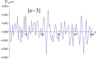
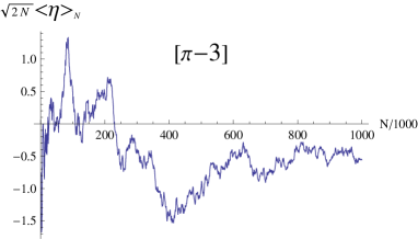
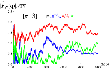
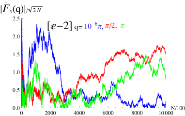
Figure 1: Plots of some quantities relevant to the SDFs obtained by the Wiener models associated to the transcendent numbers $(\pi-3)$ and $(e-2)$, numerically evaluated up to the $2N=10^{6}$th binary digit. [The horizontal axis label should read $2N/1000$ instead of the the reported $N/1000$.]

This relation not only confirms that the mean value of the SDF $\eta(x)$, as expected, vanishes, but it also shows that, as stated by Ciccariello (2017), it vanishes as $|\nu|/\sqrt{2L}$ with $|\nu|=1$.
We have tried to numerically test the validity of (94) and (92). To this aim we considered the cases $\alpha=(\pi-3)$ and $\alpha=(e-2)$ and evaluated their binary representations up to the $2N$th$=10^{6}$th binary digit. The corresponding $\eta_{k}$s are obtained by (83) which also yields the analytic expression of $\eta(x)$ for $-N<x\leq N$. Knowing $\eta(x)$ it is numerically straightforward to evaluate the $\gamma_{N}(m)$s at some integer $m$ values, the mean value ${\langle\eta\rangle}_{N}$ of $\eta(x)$ over the interval $[-N,/,N]$ and $|{\tilde{F}}_{N}(q)|$, defined by (86), in terms of $N$ and $q$. Figure 1 shows the obtained results. The top left panel shows the $\gamma_{N}(m)$ values at the positive integers $m$ not exceeding 100 for the case $\alpha=(\pi-3)$. One sees that the values fluctuate around zero and the largest deviations are of the order of $1/\sqrt{2N}=10^{-3}$. The results for the case $\alpha=(e-2)$ are quite similar. Thus, they seem to confirm Wiener’s conclusion that, in the $N\to\infty$ limit, all the $\gamma(m)$s are equal to zero whatever $\alpha$. But, this conclusion might be hurried owing to the small range of the considered $m$s. [To enlarge this range, one should consider a much larger value of $N$ and this is not numerically easy owing to the exponential increase of the computation time.] The top right panel plots $\sqrt{2N}{\langle\eta\rangle}_{N}$ versus $N$ in the range $1\leq 2N\leq 10^{6}$. The tail of the curve shows an indication of a constant behavior and the same happens for the choice $(e-2)$, not shown in the figure. In the two cases, the constants look to be $1/2$ and 0 and differ, therefore, from the value 1 reported in equation (94). This fact indicates that either the considered $2N$ value is not yet asymptotic or that Wiener equation (82) does not hold true for all the irrational $\alpha$s. The bottom left panel plots the quantity $|{\tilde{F}}_{N}(q)|/\sqrt{2N}$, evaluated for the $q$ values reported in the figure (the colors of the values are those of the associated curves), versus $N$. The blue curve practically coincides with the absolute value of the curve shown in the top right panel because the last curve is associated to $q=0$ which is close to $q=\pi/10^{6}$. Finally, the bottom right panel shows the behavior of $|{\tilde{F}}_{N}(q)|/\sqrt{2N}$ for the same $q$ values, but it refers to the binary representation of $(e-2)$. It is not fully evident that the tails of all the considered $|{\tilde{F}}_{N}(q)|/\sqrt{2N}$ curves asymptotically show a constant behavior. If one inclines towards the affirmative answer, one would conclude that the constants are not equal to 1, as required by (93), and the concern about Wiener result would be confirmed. Oppositely, one would only conclude that $2N$ is not yet sufficiently large to reach the asymptotic region where all the $|{\tilde{F}}_{N}(q)|/\sqrt{2N}$ s coincide with 1. In any case, the important point is that the bottom panels of Fig. 1 numerically show that the ratios $|{\tilde{F}}_{N}(q)|/\sqrt{2N}$ neither diverge nor tend to zero. They look to tend to finite values, depending on $q$, as required by (79). According to S₁, the resulting scattering intensity must obey (80). We already saw in (91) that the sum rule is obeyed if if $\nu(q)=\lim_{N\to\infty}|{\tilde{F}}_{N}(q)|/\sqrt{2N}=1$. On the contrary, if $\nu(q)$ is a periodic function of $q$, condition (80) converts into

$$\int_{-\infty}^{\infty}I(q)dq=\int_{-\infty}^{\infty}\frac{\sin^{2}(q/2)}{(q/2)^{2}}\nu^{2}(q)dq=2\pi.$$

We are certain that the last integral converges but the poor numerical accuracy in the $\nu(q)$ knowledge does not allow a reliable check of the relation.

4.2 Another model

We numerically analyze now another model of the Méring-Tchoubar kind but not of Wiener’s. We again assume that the scattering densities of particles and voids are equal to 1 and -1, that particle 1 has the left border at the origin $O$ and that $\eta(x)$ is an even function. Thus, to fully characterize the model, it is sufficient to assign the lengths of particles and voids in the only region $x>0$. The lengths of the particles and the voids are assigned according to the following definitions

$$d_{k}\equiv a+\Delta_{k},\quad z_{k}\equiv a,\quad\Delta_{k}\equiv\frac{b}{\sqrt{c^{2}+k(1-\cos k)}},\quad k=1,2,\ldots$$ (95)

where $a$, $b$ and $c$ are positive numbers, later specified.

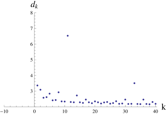
Figure 2: Plot of the first 40 $d_{k}$ values, in units $u$, for the case $a=2,\,b=1,\,c=1/100$.

The greatest lower bounds of the $d_{k}$s and the $z_{k}$s are equal to $a$, but the ratios $d_{k}/a$ are not integers. This makes the model different from Wiener’s. The essential ingredient is contribution $\Delta_{k}$ present in the $d_{k}$ definition. Since $0\leq(1-\cos x)\leq 2$, it happens that $k(1-\cos k)$ is close to zero at some particular $k$s that can also be arbitrarily large. This property makes the $d_{k}$ values random, even though they obey the inequalities $a<d_{k}<a+b/c$. Besides, it ensures a stronger homogeneity in comparison to the case where contribution $\cos k$ is omitted in the $d_{k}$ definition, because comparatively large $d_{k}$s can also be met at large $k$ values. For illustration, the first 40 $d_{k}$ values for the case $a=2,\,b=1,\,c=10^{-2}$ are shown in figure 2.
The particle $(\varphi_{1})$ and void volume ($\varphi_{2}$) fractions are obtained evaluating the sums of particle and void lengths up to the $N$th void, i.e.

$$D_{N}=\sum_{k=1}^{N}d_{k}=Na+{\cal D}_{N},\quad Z_{N}=Na,\quad{\cal D}_{N}\equiv\sum_{k=1}^{N}\Delta_{k},$$ (96)

and taking the limit $N\to\infty$ of the appropriate ratios, i.e.

$$\varphi_{1}=\lim_{N\to\infty}\varphi_{1,N}\equiv\lim_{N\to\infty}\frac{Na+{\cal D}_{N}}{2Na+{\cal D}_{N}},$$ (97)

$$\varphi_{2}=\lim_{N\to\infty}\varphi_{2,M}\equiv\lim_{N\to\infty}\frac{Z_{N}}{2Na+{\cal D}_{N}}.$$

Since $\varphi_{1,N}+\varphi_{2,N}=1$, the expected relation $\varphi_{1}+\varphi_{2}=1$ is obviously obeyed. A rough estimation of the way ${\cal D}_{N}$ depends on $N$ at large $N$s can be obtained substituting, in the $\Delta_{k}$ definition, the factor $(1-\cos k)$ with a positive constant $C$, representing a sort of mean value, and converting the ${\cal D}_{N}$ expression into an integral. In this way one finds

$${\cal D}_{N}\approx\sum_{k=1}^{N}\frac{b}{\sqrt{c^{2}+Ck}}\approx\int_{0}^{N}\frac{b}{\sqrt{c^{2}+Cx}}dx=$$

$$\quad\quad\frac{2b}{C}\bigl{[}\sqrt{c^{2}+CN}-c\bigr{]}\approx 2b(N/C)^{1/2}+o.$$ (98)

This relation shows that ${\cal D}_{N}$ linearly increases with $N^{1/2}$ and from (97) one obtains that $\varphi_{1}=\varphi_{2}=1/2$. By equations (96) and (4.2 Another model) it is also possible to determine how the mean value of the considered SDF over the interval of length $L_{N}[\equiv(2Na+{\cal D}_{N})]$ behaves as $N$ increases.

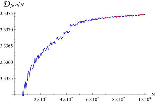
Figure 3: Plot of quantity ${\cal D}_{N}$ (defined by (96) and in units $u$) relevant to $N$ subsequent particle-void pairs and divided by $N^{1/2}$, versus $N$. The broken red curve approaches the constant value A=13.84 (see text).

One finds

$$\langle\eta\rangle_{L_{N}}=\frac{1}{L_{N}}\int_{0}^{L_{N}}\eta(x)dx=\frac{{\cal D}_{N}}{2Na+{\cal D}_{N}}\approx\frac{b}{a\sqrt{CN}}+o,$$ (99)

i.e.  once more the expected $L^{-1/2}$ behavior. It is possible to numerically determine the constant $A\equiv\frac{b}{a\sqrt{C}}$ present in (99). To this aim, one first evaluates the ${\cal D}_{N}$s over a large set of $N$values and then one fits the expression $A+B/\sqrt{N}$ to the evaluated ${\cal D}_{N}/\sqrt{N}$ values. Fig. 3 shows these values (calculated with $b=1,\,c=10^{-2}$ within the range $1\leq N\leq 10^{8}$) as well as, in red, the resulting fitting curve over the best-fitted $N$ range. By the best-fit one finds that $A=13.8401$ (and $B=0.000095$).
The FT of $\eta(x)$, evaluated over the interval centered at the origin $O$ and containing $2N$ particle/void pairs [$N$ pairs on the left and $N$ on the right of $O$], reads

$${\tilde{\eta}}_{N}(q)=(4/q)\sum_{k=1}^{N}\Bigl{\{}\cos[q(L_{k-1}+d_{k}/2)]{\sin(qd_{k}/2)}-$$

$$\quad\quad\quad\quad\cos[q(L_{k-1}+d_{k}+z_{k}/2)]{\sin(qz_{k}/2)}\Bigr{\}},$$ (100)

where we have used the eveness of $\eta(\cdot)$ and put $L_{0}=0$.
Figure 4 shows the behavior of ${\tilde{\eta}}_{N}(q)/L_{N}$ in terms of $N$ for some of the typical $q$ values that we choose to consider.

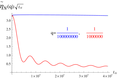
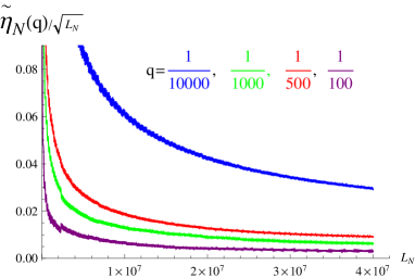
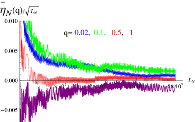
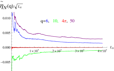
Figure 4: Plots of ${\tilde{\eta}}_{N}(q)/\sqrt{L_{N}}$ (in a.u.) versus $N$ for different values of $q$ reported in each panel.

All the panels refer to $N$ values ranging from 1 to $4\times 10^{7}$. The shown values of $|{\tilde{\eta}}_{N}(q)|/\sqrt{L_{N}}$ refer to $N$s spaced by $10^{3}$. This could make the real oscillations of the plotted quantity wider than it appears from the figures. This should not happen because the evaluation was also performed over the last $10^{3}$ values of $N$ with a unit spacing and the oscillations are of the size present in the curve tails. In each panel, the curve of a given color refers to the $q$ value of the same color. All the shown curves indicate that, as $N$ becomes sufficiently large, $|{\tilde{\eta}}_{N}(q)|/\sqrt{L_{N}}$ approaches to a constant, the value of which depends on $q$. In this way, relation (79) appears numerically to be obeyed. The square of the $|{\tilde{\eta}}_{N}(q)|/\sqrt{L_{N}}$ value at the largest $N$ value yields a numerical approximation of the scattering intensity. Fig. 5 shows the corresponding values in a log-log plot for all the $q$ values that we have considered. The resulting shape conforms to those usually met in SAS. The oscillations present in the tail region are likely related to the fact that most of the particles and voids have size close to 2. In fact, the three smallest intensities are found at $q=\pi,\,2\pi,\,4\pi u^{-1}$. These oscillations and the small numerical values of the intensities make hard to numerically ascertain that sum-rule (80) is obeyed. Aside from this point numerically not assessed, all the other results conform to (79) so that one can, somewhat confidently, conclude that the $\eta(x)$ defined by (95) is a SDF.

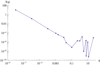
Figure 5: Log-log plot of the scattering intensity versus $q$ for the Méring-Tchoubar model defined by (95) with $a=2,\,b=1,\,c=10^{-2}$. The intensity units are arbitrary and those of $q$ are $u^{-1}$, $u$ being the unit length used to define the particles’ and voids’ sizes.

Conclusions

The above analysis leans upon Wiener results and assumptions A, B and C  that are suggested by experimental results. It has been shown that assumption C combined with Wiener analysis leads to the mathematical characterization of SDFs through statement S₂. In this way, any $\eta(x)\in{{\cal W}_{p}}$ can be considered a SDF because it generates, via definitions (16) and (21), a CF $\gamma(x)$ continuous throughout $R$ and such that the associated Fourier integral $\sigma(q)$, defined by equation (49), is a non-decreasing and absolutely continuous function. Besides, the resulting $\gamma(x)$ is an $L_{2}$ function and the scattering intensity simply is its Fourier transform. It has also been shown that the condition ensuring that an $\eta(x)$ is a SDF can be formulated according to statement S₁, i.e. that $\eta(x)$ must be such that the limit (79) exists for any $q$ and it is such that sum rule (80) also is obeyed.
We are aware that both procedures of defining physical SDFs are, on a practical ground, hard to be applied since they are, to a large extent, of implicit nature. Therefore they need further theoretical exploitation to get more direct constraints on the $\eta(x)$s eligible to be physical SDFs. From this point of view, our analysis only showed that $\eta(x)$ must be bounded, have a behavior irregularly oscillating around zero and not to contain contributions of the form $\sum_{J}A_{j}\cos(\alpha_{j}x)$ with the $\{A_{j}\}$s finite. The further mathematical constraints on $\eta(x)$ that ensure the continuity and the $L_{2}$ summability of the associated $\gamma(x)$ are still unknown even though it is physically plausible that they should involve some probability-theory aspects as yet poorly defined. In fact, the Méring-Tchoubar models that we have numerically analyzed contain some of these elements. The corresponding results indicate that the ${{\cal W}_{p}}$ set is not void as well as the necessity of considering larger $N$ values for the results obtained by numerical computations may be fully trusted.

Acknowledgmets

S.C. is grateful to Professors P. Ciatti, K. Lechner and M. Matone for useful conversations.

References

Borel, E. (1909). Rend. Circ. Mat. Palermo XXVII, 247-271.

Chandrasekharan, K. (1980). Classical Fourier Transforms. Berlin: Springer-Verlag.

Cervellino, A. & Ciccariello, S. (2001). J. Phys. A: Math. Gen. 34, 731-755.

Ciccariello, S. (2017). J. Appl. Cryst. 50, 594-601.

Ciccariello, S. (2005). Prog. Colloid Polym. Sci. 130, 20-28.

Debye, XYZ., Anderson, H.R. & Brumberger, H. (1957). J. Appl. Phys. 20, 679-683.

Feigin, L.A. & Svergun, D.I. (1987). Structure Analysis by Small-Angle X-Ray and Neutron Scattering, New York: Plenum Press.

Gradshteyn, I.S. & Ryzhik, I.M. (1980). Table of Integrals, Series, and Products, New York: Academic Press.

Guinier, A. (1952). X-Ray Diffraction: In Crystals, Imperfect Crystals, and Amorphous Bodies New York: Dover.

Guinier, A. & Fournet, G. (1955). Small-Angle Scattering of X-rays. New York: John Wiley.

Kolmogorov, A.N. & Fomin, S.V. (1980) Elementi di teoria delle funzioni e di analisi funzionale, Mosca: Ediz. MIR.

Mahler, K. (1927). J. Math. Phys. Mass. Inst. Technology 6, 158-164.

Méring, J. & Tchoubar, D. (1968). J. Appl. Cryst. 1, 153-65.

Morita, T. & Hiroike, K. (1961). Prog. Theor. Phys. 25, 537-592.

Plancherel, M. (1915). Math. Ann. 7, 315-326.

Porod, G. (1951). Kolloid Z. 124, 83-114.

Schuster, A. (1906). Proc. Roy. Soc. 17, 136-140.

Wiener, N. (1930). Acta Math. 30, 118-242.

Wiener, N. (1933). The Fourier Integral and Certain of Its Applications, New-York: Dover Pub. Inc.