The orbit method and analysis of automorphic forms

Abstract.

We develop the orbit method in a quantitative form, along the lines of microlocal analysis, and apply it to the analytic theory of automorphic forms.

Our main global application is an asymptotic formula for averages of Gan–Gross–Prasad periods in arbitrary rank. The automorphic form on the larger group is held fixed, while that on the smaller group varies over a family of size roughly the fourth root of the conductors of the corresponding $L$-functions. Ratner’s results on measure classification provide an important input to the proof.

Our local results include asymptotic expansions for certain special functions arising from representations of higher rank Lie groups, such as the relative characters defined by matrix coefficient integrals as in the Ichino–Ikeda conjecture.

1. Introduction

The problem of giving asymptotic formulas for moments of large degree $L$-functions has proved challenging. In approaching this problem, one encounters difficult analytic questions in the representation theory of reductive Lie groups, involving complicated multi-dimensional oscillatory integrals.

The orbit method (see, e.g., [Kir2, Vo3]) is a philosophy for, among other purposes, reducing difficult problems in the representation theory of Lie groups to simpler problems in symplectic geometry. It has been widely applied in the algebraic side of that theory.

This paper develops the orbit method in a quantitative analytic form. We combine the tools thus developed with an indirect application of Ratner’s theorem to study moments of automorphic $L$-functions on higher rank groups.

1.1. Overview of results

We refer the reader who is not familiar with automorphic forms to §1.3 and onwards for an introduction, in explicit terms, to the main ideas of this paper.

Let $\mathbf{H}\hookrightarrow\mathbf{G}$ be an inclusion of reductive groups over a number field $F$. Let $\Pi$ and $\Sigma$ be cuspidal automorphic representations of $\mathbf{G}$ and $\mathbf{H}$, respectively. Assuming that $\mathbf{H}\hookrightarrow\mathbf{G}$ is a strong Gelfand pair, and under a temperedness assumption, one may define an “automorphic branching coefficient” $\mathcal{L}(\Pi,\Sigma)\geqslant 0$ which quantifies how vectors in $\Pi$ correlate with $\Sigma$. We recall this definition in a simple setting in §1.4 and more fully in §7.4.

We focus on the “Gan–Gross–Prasad” case (§13) in which

$$(\mathbf{G},\mathbf{H}) (\mathrm{SO}_{n},\mathrm{SO}_{n-1}) (\mathrm{U}_{n},\mathrm{U}_{n-1})$$ is a form of either or .

The definition of $\mathcal{L}(\Pi,\Sigma)$ then applies, at least for tempered $\Pi$ and $\Sigma$, and one expects $\mathcal{L}(\Pi,\Sigma)$ to be related to special values of $L$-functions: Ichino–Ikeda [II] and N. Harris [Har2] conjecture the formula

$$\mathcal{L}(\Pi,\Sigma)=2^{-\beta}\frac{L^{(R)}(\frac{1}{2},-,\Pi\times\Sigma^{\vee})}{L^{(R)}(1,\mathrm{Ad},\Pi\times{\Sigma}^{\vee})}\Delta_{G}^{(R)},$$ (1.1)

whose terms are as follows (see loc. cit. for details):

• $R$ is a fixed set of places outside of which $\Pi$ and $\Sigma$ are spherical. (Thus $\mathcal{L}(\Pi,\Sigma)$ depends upon $R$.)

• $\Sigma^{\vee}$ denotes the contragredient of the unitary representation $\Sigma$; it is isomorphic to the conjugate representation $\overline{\Sigma}$, and we will occasionally use the latter notation.

• $L^{(R)}$ denotes an $L$-function without Euler factors in $R$.

• $2^{\beta}$ is the size of the Arthur component group of $\Pi\boxtimes\Sigma^{\vee}$ on $\mathbf{G}\times\mathbf{H}$.

• $\Delta_{G}$ is the $L$-function whose local factor at almost every prime $p$ equals $\frac{p^{\dim(G)}}{\#\mathbf{G}(\mathbf{F}_{p})}$ (see [Gr]); e.g., $\Delta_{G}=\zeta(2)\zeta(4)\dots\zeta(2n)$ for $G=\mathrm{SO}_{2n+1}$; $\Delta_{G}^{(R)}$ omits factors at $R$.

The formula (1.1) has been proved in the unitary case, under local assumptions which allow one to use a simple form of the trace formula, by W. Zhang [Z2] (see also [Z1, §2.2] and [Beu3]).

Fix one such $\Pi$. What are the asymptotic statistics of $\mathcal{L}(\Pi,\Sigma)$, as $\Sigma$ varies over a large family? For example, what are the moments? Predictions for these may be obtained via (1.1) and random matrix heuristics (§1.2) for families of $L$-functions. To verify such predictions rigorously has proved an interesting challenge, testing our understanding of families of automorphic forms and $L$-functions. It has been successfully undertaken in many low-degree cases, where obtaining strong error estimates remains an active area of research (see, e.g., [BFKMM, BM, KMS, BFKMMS] and references).

We aim here to explore some first cases of arbitrarily large degree. Our main result (theorem 25) may be summarized informally as follows:

Theorem.

Assume certain local conditions, including the compactness of the quotients $\mathbf{G}(F)\backslash\mathbf{G}(\mathbb{A})$ and $\mathbf{H}(F)\backslash\mathbf{H}(\mathbb{A})$. For each sufficiently small positive real $\operatorname{h}$, let $\mathcal{F}_{\operatorname{h}}$ be the family of all $\Sigma$ as above which are locally distinguished by $\Pi$, have Satake parameters at some fixed archimedean place inside the rescaling $\operatorname{h}^{-1}\Omega$ of some nice fixed compact set $\Omega$, and have “fixed level” at the remaining places in $R$. Then the branching coefficient $\mathcal{L}(\Pi,\Sigma)$, averaged over $\Sigma\in\mathcal{F}_{\operatorname{h}}$, is asymptotic to $1/2$:

$$\lim_{\operatorname{h}\rightarrow 0}\frac{1}{|\mathcal{F}_{\operatorname{h}}|}\sum_{\Sigma\in\mathcal{F}_{\operatorname{h}}}\mathcal{L}(\Pi,\Sigma)=\frac{1}{2}.$$ (1.2)

For “typical” $\Pi$ and $\Sigma$, we expect that (1.1) holds with $\beta=2$ (see §7.5 for further explanation). Our result should thus translate, under (1.1), as follows:

$$\text{The average value of $\frac{L^{(R)}(\frac{1}{2},-,\Pi\times\Sigma^{\vee})}{L^{(R)}(1,\mathrm{Ad},\Pi\times{\Sigma}^{\vee})}\Delta_{G}^{(R)}$ is $2$}.$$ (1.3)

We outline in §1.2 why (1.3) agrees with random matrix theory heuristics for orthogonal families of $L$-functions with positive root number.

One way to normalize the strength of (1.2) is to note (§13.4) that the size of the family $\mathcal{F}_{h}$ is roughly the fourth power of the analytic conductor of the relevant $L$-function. By ignoring all but one term and slowly shrinking the family, we obtain a “weakly subconvex” bound

$$\mathcal{L}(\Pi,\Sigma)=o\left(\mathrm{cond}(\Pi\times\Sigma)^{1/4}\right)$$ (1.4)

(compare with [Sou, SoTh]). The hypotheses relevant for (1.4) are that $\Pi$ is fixed, while $\Sigma$ traverses a sequence whose archimedean Satake parameters all tend off to $\infty$ at the same rate.

The new ideas used to obtain (1.2) are based on the orbit method, applied in two ways:

• Firstly, to determine the asymptotics of complicated oscillatory integrals on higher rank groups. For instance, theorem 15 gives general and uniform asymptotic expansions of relative characters away from the conductor-dropping locus. This analysis gives a robust supply of analytic test vectors for the local matrix coefficient integrals as in Ichino–Ikeda. We hope these to be of general use in analytic problems involving families of automorphic forms in higher rank.

• Secondly, to obtain invariant measures towards which we can apply measure-theoretic techniques. Indeed, a major global ingredient for (1.2) is an application of Ratner’s theorem to the case of measures invariant by the centralizer of a regular nilpotent element in $\mathbf{G}(F)$. The estimate (1.2) is ineffective, and the application of Ratner is solely responsible for the ineffectivity. We expect that an effective version of Ratner’s theorem for the case at hand would lead to a subconvex estimate for $\mathcal{L}(\Pi,\Sigma)$; this perhaps contributes interest to the problem of effectivization.

To implement these, we develop a microlocal calculus for Lie group representations, which may be understood as a quantitative, analytic form of the orbit method and the philosophy of geometric quantization.

These basic ideas do not interact with the arithmetic nature of the setting; in particular, we do not use Hecke operators. However, the problem of averaging and bounding $L$-functions seems to be the most interesting source of applications at the moment.

1.2. Compatibility with random matrix heuristics

We briefly outline why our result (1.3) should be compatible with the standard heuristics.

Random matrix theory heuristics (see, e.g., [BK] and references, such as [KaSa, CF, CFKRS, KeSn1, KeSn2]) suggest, for a family of $L$-functions $L(\frac{1}{2},f)$ parameterized by elements $f$ of some nice enough family $\mathcal{F}$, that

$$\frac{1}{|\mathcal{F}|}\sum_{\mathcal{F}}L^{(R)}(\tfrac{1}{2},f)\approx\left(\mbox{global factor $g$}\right)\times\prod_{p}\langle a_{p}\rangle$$

where

• $p$ runs over the finite primes of $F$ outside $R$,

• $\langle a_{p}\rangle$ is the expectation

  $$\langle a_{p}\rangle:=\frac{1}{|\mathcal{F}|}\sum_{\mathcal{F}}L_{p}(\tfrac{1}{2},f)$$

  of the central value of the $p$th Euler factor, and

• the “global factor” $g$ is described by random matrix theory, and given here by the following limit of integrals taken with respect to probability Haar measures:

  $$g=\lim_{N\rightarrow\infty}\int_{x\in\mathrm{SO}(2N)}\det(1-x).$$

  Indeed, the symmetry type [KaSa] of the family of $L$-functions implicit in (1.2) is $O(2N)$, i.e., it is an orthogonal family with positive root numbers. One may see this by, for instance, considering the analogous situation with the number field replaced by a function field (see also [ShTe, SST]).

Each integral $\int_{\mathrm{SO}(2N)}\det(1-x)$ equals $2$, independent of $N$. Indeed, $\det(1-x)$ is the (super-)trace of $x\in\mathrm{SO}(2N)$ on $\wedge^{*}(\mathbb{C}^{2N})$. The average trace of $x$ on $\wedge^{j}(\mathbb{C}^{2N})$ computes the dimension of invariants, which is $1$ for $j\in\{0,2N\}$ and $0$ otherwise. Thus $g=2$.

We sketch here why $\langle a_{p}\rangle=1$ for every $p$. We expect the families $\mathcal{F}_{\operatorname{h}}$ considered here to have the (provable) property that the local component $\sigma_{p}$ at $p$ of a uniformly random element $\Sigma\in\mathcal{F}_{\operatorname{h}}$ becomes distributed, as $\operatorname{h}\rightarrow 0$, according to the Plancherel measure $d\sigma_{p}$, thus

$$\langle a_{p}\rangle=\int_{\sigma_{p}}\underbrace{\frac{L_{p}(\frac{1}{2},-,\pi_{p}\times\sigma_{p}^{\vee})}{L(1,\mathrm{Ad},\pi_{p}\times\sigma_{p}^{\vee})}\Delta_{G,p}}_{=:I(\pi_{p},\sigma_{p})}\,d\sigma_{p}.$$

Ichino and Ikeda [II, Theorem 1.2] have shown in the orthogonal case, and N. Harris [Har2, Theorem 2.12] in the unitary case, that this integral can be rewritten as a matrix coefficient integral: $I(\pi_{p},\sigma_{p})=\int_{h\in H_{p}}\langle hv,v\rangle\langle u,hu\rangle dh$, where $v\in\pi_{p}$ and $u\in\sigma_{p}$ are spherical unit vectors and $dh$ is the Haar measure assigning unit volume to a hyperspecial maximal compact subgroup. Using the Plancherel formula, one can show (§18) that $\int_{\sigma_{p}}I(\pi_{p},\sigma_{p})d\sigma_{p}=1$, as required.

We have not discussed yet the quantity $\beta$ as in (1.1). As mentioned above, we expect for “typical” $\Pi$ and $\Sigma$ that $\beta=2$. However, for “atypical” $\Pi$ (i.e., endoscopic lifts), one can have $\beta>2$ in the entire family. In that case, the limit of (1.3) is instead a larger power of $2$. Correspondingly, the $L$-function in question factors. It seems to us that our result continues to match with $L$-function heuristics after appropriately accounting for this factorization and variation of root numbers, but we have not checked all details.

The random matrix theory predictions for higher moments involve somewhat more complicated coefficients than the quantity $g=2$ appearing above. It may be possible to study higher moments by adapting our method to periods of Eisenstein series, and would be interesting to obtain in that way some geometric perspective on those predictions.

1.3. Basic setup

We now simultaneously outline the contents of this paper and sketch the main arguments.

Suppose given a pair of unimodular Lie groups $G$ and $H$, with $H\leqslant G$. An example relevant for our main theorem is when

$G$ and $H$ are the real points of the split forms of $\mathrm{SO}_{n+1}$ and $\mathrm{SO}_{n}$.

We assume that representations of $G$ have “multiplicity-free restrictions” to $H$, as happens in the indicated example (see [SZ] for a precise statement and proof).

Suppose also given a lattice $\Gamma$ in $G$ for which $\Gamma_{H}:=\Gamma\cap H$ is a lattice in $H$. We assume that both quotients

$$[G]:=\Gamma\backslash G,\quad[H]:=\Gamma_{H}\backslash H$$

are compact. We equip them with Haar measures.

For the motivating applications to $L$-functions, we must consider adelic quotients. This entails some additional work at “auxiliary places” (see §6) which we do not discuss further in this overview.

1.4. Branching coefficients: comparing global and local restrictions

Let

$$\pi\subseteq L^{2}([G])$$

be an irreducible unitary subrepresentation, with the group $G$ acting by right translation. We assume that $\pi$ is tempered. The branching coefficients of interest arise from comparing the two natural ways to restrict $\pi$ to $H$:

• (Globally) Take a smooth vector $v\in\pi$. It defines a function on $[G]$. We may restrict it to obtain a function $v|_{[H]}$ on $[H]$. The $L^{2}$-norm of that restriction may be decomposed as

  $$\int_{[H]}|v|^{2}=\sum_{\text{irreducible }\sigma\subseteq L^{2}([H])}\|\mbox{projection of $v|_{[H]}$ to $\sigma$}\|^{2}.$$ (1.5)

• (Locally) Consider $\pi$ as an abstract unitary representation of $G$. We may restrict it to obtain an abstract unitary representation $\pi|_{H}$ of $H$. We verify in the examples of interest (see §18) that this restriction decomposes as a direct integral

  $$\pi|_{H}=\oint_{\sigma}m_{\sigma}\sigma,$$

  weighted by multiplities $m_{\sigma}\in\{0,1\}$, and taken over tempered irreducible unitary representation $\sigma$ of $H$ with respect to Plancherel measure. We may define the components $\mathrm{pr}_{\sigma}(v)\in\sigma$ of a smooth vector $v\in\pi$ with respect to this decomposition, and we have

  $$\|v\|^{2}=\int_{\sigma}\|\mathrm{pr}_{\sigma}(v)\|^{2}.$$ (1.6)

  A priori, $\|\mathrm{pr}_{\sigma}(v)\|$ is defined only as a measurable function of $\sigma$, but there is a natural way to define it pointwise in the cases of interest.

Let $\sigma\subseteq L^{2}([H])$ be an irreducible tempered subrepresentation for which $m_{\sigma}=1$; we refer to such $\sigma$ as $\pi$-distinguished. By the multiplicity one property, we may define a proportionality constant $\mathcal{L}(\pi,\sigma)\geqslant 0$ by requiring that for every smooth vector $v\in\pi$,

$$\|\mbox{projection of $v|_{[H]}$ to $\sigma$}\|^{2}=\mathcal{L}(\pi,\sigma)\cdot\|\mathrm{pr}_{\sigma}(v)\|^{2}.$$ (1.7)

We note that $\mathcal{L}(\pi,\sigma)$ depends upon the choices of Haar measure.

1.5. Objective

Let $\operatorname{h}$ traverse a sequence of positive reals tending to zero, and let $\mathcal{F}_{\operatorname{h}}$ be a corresponding sequence of families consisting of irreducible tempered representations $\sigma\subseteq L^{2}([H])$ for which $m_{\sigma}=1$.

We assume that each family $\mathcal{F}_{\operatorname{h}}$ arises from some nice subset $\tilde{\mathcal{F}_{\operatorname{h}}}$ of the $\pi$-distinguished tempered dual of $H$ as the set of all irreducible $\sigma\subseteq L^{2}([H])$ for which the class of $\sigma$ belongs to $\tilde{\mathcal{F}_{\operatorname{h}}}$. We assume that $|\mathcal{F}_{\operatorname{h}}|\rightarrow\infty$ as $\operatorname{h}\rightarrow 0$. (In our main theorem, we take for $\tilde{\mathcal{F}_{\operatorname{h}}}$ the set of $\sigma$ whose infinitesimal character belongs to the rescaling $\operatorname{h}^{-1}\Omega$ of some fixed nonempty bounded open set $\Omega$.) Our aim is to determine the asymptotics of the sums

$$\sum_{\sigma\in\mathcal{F}_{\operatorname{h}}}\mathcal{L}(\pi,\sigma).$$

In our motivating examples, these are (in some cases conjecturally) proportional to sums of special values of $L$-functions.

We drop the subscript $\operatorname{h}$ in what follows for notational simplicity.

1.6. Strategy

The rough idea of our proof is to find a vector $v\in\pi$ which simultaneously “picks out the family $\mathcal{F}$” in that

$$\|\mathrm{pr}_{\sigma}(v)\|^{2}\approx\begin{cases}1&\text{ if }\sigma\in\tilde{\mathcal{F}},\\ 0&\text{ if }\sigma\notin\tilde{\mathcal{F}}\end{cases}$$ (1.8)

and “becomes equidistributed” in that

$$\frac{\int_{[H]}|v|^{2}}{\mathrm{vol}([H])}\sim\frac{\int_{[G]}|v|^{2}}{\mathrm{vol}([G])}.$$ (1.9)

The vector $v$ will of course depend upon the family $\mathcal{F}=\mathcal{F}_{\operatorname{h}}$, hence upon the asymptotic parameter $\operatorname{h}>0$, and the above estimates are to be understood as holding asymptotically in the $\operatorname{h}\rightarrow 0$ limit. Note that (1.8) is a purely local problem of harmonic analysis in the representation $\pi$, whereas (1.9) is a global problem: it relates to the specific way in which $\pi$ is embedded in $L^{2}([G])$.

The Weyl law on $[H]$ says that the cardinality of $\mathcal{F}$ is approximately the volume of $[H]$ times the Plancherel measure of $\tilde{\mathcal{F}}$, thus by (1.8) and (1.6),

$$|\mathcal{F}|\approx\mathrm{vol}([H])\|v\|^{2}.$$ (1.10)

Comparing (1.5), (1.7) and (1.8) with (1.10) yields the required asymptotic formula

$$\frac{1}{|\mathcal{F}|}\sum_{\sigma\in\mathcal{F}}\mathcal{L}(\pi,\sigma)\sim\frac{1}{\mathrm{vol}([G])}.$$ (1.11)

In applications, the volumes are defined using Tamagawa measure and given then by $\mathrm{vol}([H])=\mathrm{vol}([G])=2$. Thus (1.11) leads to (1.2).

Observe, finally, that it suffices to produce families of vectors $v_{i}\ (i\in I)$ for which the analogues of (1.8) and (1.9) hold on average over the index set $I$.

We note that this basic strategy has appeared (sometimes implicitly) in several antecedent works (see, e.g., [Sar, BR2, Ve, MV]). We would like to note, in particular, the influence of the ideas of Bernstein and Reznikov in exploiting the uniqueness of an invariant functional. The novelty here is that we execute this strategy successfully in arbitrarily large rank.

1.7. Microlocal calculus for Lie group representations

To implement this strategy, we need some way to produce and analyze (families of) vectors in the representation $\pi$. Our approach, inspired by microlocal analysis, is to work with vectors implicitly through their symmetry properties under group elements $g\in G$ within a suitable shrinking neighborhood of the identity element. Since we do not expect our readers to have extensive prior familiarity with microlocal analysis, we describe here its content in our setting. The discussion in this section is rather informal, but we hope that the reader will find it helpful in navigating the many technical estimates of the text.

The shrinking neighborhood in question depends upon an infinitesimal scaling parameter $\operatorname{h}\rightarrow 0$. Let $\mathfrak{g}$ denote the Lie algebra of $G$, and $\mathfrak{g}^{\wedge}$ the Pontryagin dual of $\mathfrak{g}$; we identify $\mathfrak{g}^{\wedge}$ with the imaginary dual $i\mathfrak{g}^{*}$, and denote by $e^{x\xi}\in\mathbb{C}^{(1)}$ the image of $(x,\xi)\in\mathfrak{g}\times\mathfrak{g}^{\wedge}$ under the natural pairing. Informally, we say that a vector $v\in\pi$ is microlocalized at $\xi\in\mathfrak{g}^{\wedge}$ if

$$\pi(\exp(x))v\approx e^{x\xi/\operatorname{h}}v$$ (1.12)

for all $x\in\mathfrak{g}$ of size $|x|=\operatorname{O}(\operatorname{h})$. In practice, we choose $\operatorname{h}$ small enough in terms of $\pi$ that such vectors exist. For instance, if $\pi$ is generated by a Maass form $\varphi$ of Laplace eigenvalue $\lambda$ on a locally symmetric space $\Gamma\backslash G/K$, then we choose $\operatorname{h}$ comparable to or smaller than the “wavelength scale” $|\lambda|^{-1/2}$ of $\varphi$; similar considerations apply more generally, with the role of wavelength scale played by the inverse root norm $|\lambda_{\pi}|^{-1/2}$ of the infinitesimal character of $\pi$ (see §9.8). We quantify the heuristic (1.12) in several different ways throughout this paper, typically by working with sequences of representations $\pi=\pi_{\operatorname{h}}$ and vectors $v=v_{\operatorname{h}}$ that vary with $\operatorname{h}$ and asking that the difference between the left and right hand sides of (1.12) decay at some specified rate as $\operatorname{h}\rightarrow 0$.

The group elements $g=\exp(x)$ with $|x|=\operatorname{O}(\operatorname{h})$ approximately commute as $\operatorname{h}\rightarrow 0$, and so the operators $\pi(g)$ may be approximately simultaneously diagonalized; their common approximate eigenvectors are the microlocalized vectors. We might thus hope for an approximate decomposition

$$\pi\approx\bigoplus_{\xi}\mathbb{C}v_{\xi},$$ (1.13)

where $\xi$ traverses a subset of $\mathfrak{g}^{\wedge}$ and $v_{\xi}\in\pi$ is microlocalized at $\xi$, and to have an approximate functional calculus

$$\mathrm{Op}_{\operatorname{h}}:\{\text{symbols $\mathfrak{g}^{\wedge}\rightarrow\mathbb{C}$}\}\rightarrow\{\text{operators on $\pi$}\},$$ (1.14)

$$\mathrm{Op}_{\operatorname{h}}(a)v_{\xi}\approx a(\xi)v_{\xi},$$ (1.15)

where “symbol” refers to a class of functions with suitable regularity.

To implement such ideas rigorously, we write down an operator assignment (1.14) and verify that it has the properties suggested by the heuristics (1.13) and (1.15). The assignment is similar to the classical Weyl calculus in the theory of pseudodifferential operators, which may be recovered (more-or-less) by specializing our discussion to standard representations of Heisenberg groups. The definition and basic properties of this assignment are philosophically unsurprising. If $a:\mathfrak{g}^{\wedge}\rightarrow\mathbb{C}$ is the Fourier mode corresponding to a small enough element $x$ in the Lie algebra of $G$, then $\mathrm{Op}_{\operatorname{h}}(a)=\pi(\exp(\operatorname{h}x))$. If $a$ is real-valued, then $\mathrm{Op}_{\operatorname{h}}(a)$ is self-adjoint. If $a$ is positive, then $\mathrm{Op}_{\operatorname{h}}(a)$ is asymptotically positive as $\operatorname{h}\rightarrow 0$. The association $a\mapsto\mathrm{Op}_{\operatorname{h}}(a)$ is nearly $G$-equivariant. One has composition formulas relating $\mathrm{Op}_{\operatorname{h}}(a)\mathrm{Op}_{\operatorname{h}}(b)$ to $\mathrm{Op}_{\operatorname{h}}(a\star_{\operatorname{h}}b)$ for a suitable star product $a\star_{\operatorname{h}}b$, bounds for operator and trace norms, and so on; see theorems 1, 2, 3, 5, 6, 7 and 9.

Our main input concerning $\pi$ is the Kirillov character formula, due in this case to Rossmann, which asserts roughly (see §12 for a precise statement) that

$$\mathrm{tr}(\mathrm{Op}_{\operatorname{h}}(a))\approx\int_{\operatorname{h}\mathcal{O}_{\pi}}a\,d\omega,$$ (1.16)

where $\mathcal{O}_{\pi}\subseteq\mathfrak{g}^{\wedge}$ is a $G$-orbit (or finite union thereof), called the coadjoint orbit attached to $\pi$. In the metaphor of microlocal analysis, the coadjoint orbit $\mathcal{O}_{\pi}$ is the “phase space” underlying $\pi$; it bears the same relationship to $\pi$ as the cotangent bundle $T^{*}M$ of a manifold $M$ does to $L^{2}(M)$. The coadjoint orbit is equipped with a canonical symplectic structure, and $d\omega$ is the associated symplectic volume form.

For each real-valued symbol $a$, we may informally identify the self-adjoint operator $\mathrm{Op}_{\operatorname{h}}(a)$ with a family of vectors $(v_{i})_{i\in I}$ by writing it in the form $\sum_{i\in I}v_{i}\otimes\overline{v_{i}}$ for some $v_{i}\in\pi$; here we have identified operators on $\pi$ with elements of (a suitable completion of) $\pi\otimes\overline{\pi}$. If the symbol $a$ is taken to be suitably concentrated near a regular point $\xi\in\mathfrak{g}^{\wedge}$, then the corresponding family is essentially a singleton (i.e., of cardinality $\operatorname{O}(\operatorname{h}^{-\varepsilon})$), consisting of vectors microlocalized at $\xi$. By decomposing the constant symbol $a=1$ associated to the identity operator $\mathrm{Op}_{\operatorname{h}}(a)=1$ and appealing to (1.16), we may write any reasonable vector as a linear combination of microlocalized vectors $v_{\xi}$, taken over representatives $\xi/\operatorname{h}$ for a partition of the coadjoint orbit $\mathcal{O}_{\pi}$ into pieces of unit symplectic volume. We may thus regard the microlocalized vectors as giving an approximate basis (1.13), with respect to which the $\mathrm{Op}_{\operatorname{h}}(a)$ act as the approximate multipliers (1.15); in other words,

$$\mathrm{Op}_{\operatorname{h}}(a)\approx\sum_{\xi\in\operatorname{h}\mathcal{O}_{\pi}}a(\xi)v_{\xi}\otimes\overline{v_{\xi}}.$$

In this way the $\mathrm{Op}_{\operatorname{h}}$-calculus parametrizes weighted families of microlocalized vectors. These considerations apply uniformly across the various classes of tempered representations of $G$ (principal series, discrete series, …) and without reference to any explicit model.

Informally, if the dominant contribution to the decomposition of a vector $v\in\pi$ as a sum $\sum v_{\xi}$ of microlocalized vectors comes from those $\xi$ belonging to some nice subset of $\operatorname{h}\mathcal{O}_{\pi}$, then we refer to that subset as the microlocal support of $v$; equivalently, it describes where the distribution on $\mathfrak{g}^{\wedge}$ given by $a\mapsto\langle\mathrm{Op}_{\operatorname{h}}(a)v,v\rangle$ is concentrated. A vector is then microlocalized if its microlocal support is concentrated near a specific point.

These notions from microlocal analysis play a central role throughout the paper, so we illustrate their content in a couple basic examples. Figure 1 depicts coadjoint orbits for certain representations $\pi$ of the groups $G=\mathrm{SO}(3)$ and $G=\mathrm{SO}(1,2)\cong\mathrm{PGL}_{2}(\mathbb{R})$, respectively; in the latter case, $\pi$ belongs to the holomorphic discrete series.

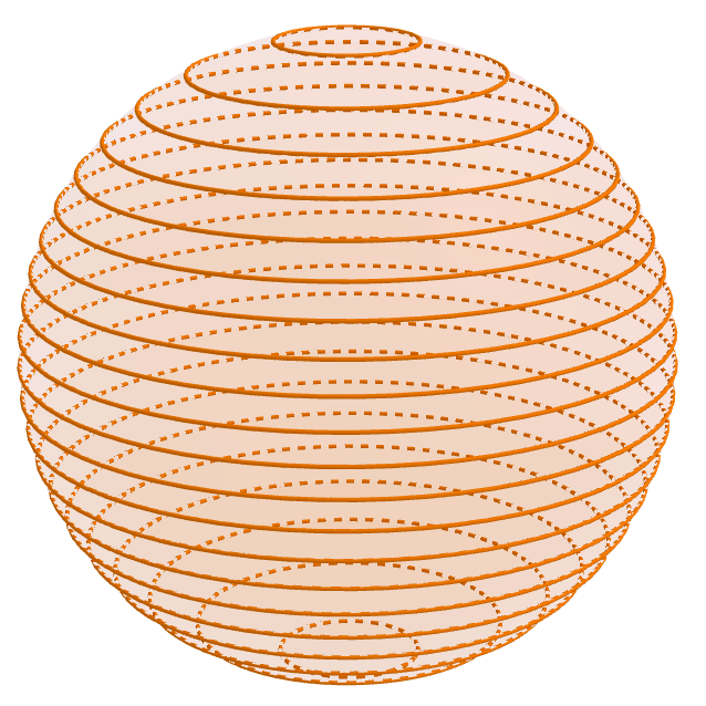
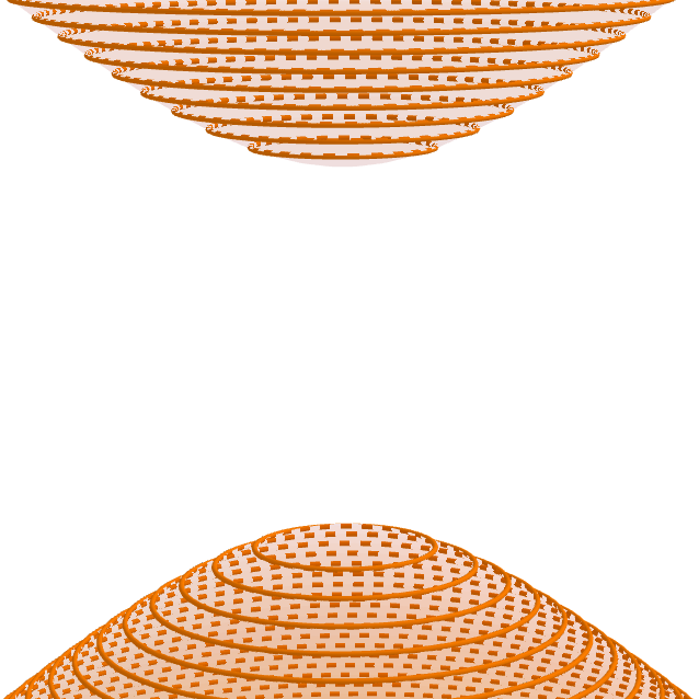
Figure 1. Coadjoint orbits for $(\mathrm{SO}_{3},\mathrm{SO}_{2})$

Each of these groups contains the compact subgroup $H=\mathrm{SO}(2)$. The circles drawn on the orbits are level sets for the “$z$-coordinate” projection $\mathfrak{g}^{*}\rightarrow\mathfrak{h}^{*}$ dual to the inclusion $\mathfrak{h}\hookrightarrow\mathfrak{g}$ of Lie algebras. They divide the orbits into strips of equal symplectic volume, say of volume $1$, which correspond under the orbit method philosophy to the basis of $\pi$ given by $H$-isotypic weight vectors $e_{n}$; the strip should be regarded as the microlocal support of the corresponding weight vector. We may normalize the weights $n$ to be even integers lying in

$$\begin{cases}[-k,k]&\text{ if }G=\mathrm{SO}(3),\\ (-\infty,-k-2]\cup[k+2,\infty)&\text{ if }G=\mathrm{SO}(1,2)\cong\mathrm{PGL}_{2}(\mathbb{R})\\ \end{cases}$$ (1.17)

for some nonnegative even integer $k$.

Let us now take $k$ tending off to $\infty$, but simultaneously zoom out our camera by the factor $k$, so that the above picture of the coadjoint orbit $\mathcal{O}_{\pi}$ remains constant. Which weight vectors should we then consider to be “microlocalized”? That is to say, for which vectors does the “zoomed out” microlocal support concentrate within some small distance of a specific point in the picture as $k\rightarrow\infty$? The strength of this notion depends upon the definition of “small distance,” which can sensibly range from the weakest scale $o(1)$ to the Planck scale $\operatorname{O}(k^{-1/2})$.

Vectors of highest or lowest weight ($e_{\pm k}$ or $e_{\pm(k+2)}$) are microlocalized, even at the Planck scale, since the corresponding strips are concentrated near the “caps” of the coadjoint orbit (i.e., the regions of extremal $z$-coordinate). By contrast, “typical” weight vectors – such as the weight zero vector $e_{0}$ in the representation of $\mathrm{SO}(3)$, corresponding to the equatorial strip – are not microlocalized, even at the weakest scale. In particular, weight vectors do not give an approximate basis of microlocalized vectors as in (1.13). The partition of the coadjoint orbit corresponding to a microlocalized basis would instead have every partition element concentrated near a specific point.

Microlocalized vectors occasionally go in the literature by other names, such as “coherent states.” They are extremely useful for the sort of asymptotic analysis pursued in this paper. Among other desirable properties, their matrix coefficients behave simply near the identity, and are as concentrated as possible; we discuss this phenomenon further in §1.10.

In the body of this paper, we do not often refer explicitly to microlocalized vectors. We instead work with them implicitly through their approximate projectors $\mathrm{Op}_{\operatorname{h}}(a)$. We hope that by phrasing the introduction in terms of microlocalized vectors, it may serve as a useful guide to the ideas behind the arguments executed in the body.

1.8. Measure classification; equidistribution

In the discussion starting in §1.7, we allowed both $\pi$ and $\operatorname{h}$ to vary simultaneously. Let us suppose now that the representation $\pi$ is held fixed, independent of the scaling parameter $\operatorname{h}$. As $\operatorname{h}\rightarrow 0$, the rescaled coadjoint orbit $\operatorname{h}\mathcal{O}_{\pi}$ then tends to a subset of the nilcone $\mathcal{N}\subseteq\mathfrak{g}^{\wedge}$. Figure 2 depicts this for the coadjoint orbits corresponding to fixed principal series representations of $G=\mathrm{SO}(1,2)\cong\mathrm{PGL}_{2}(\mathbb{R})$.

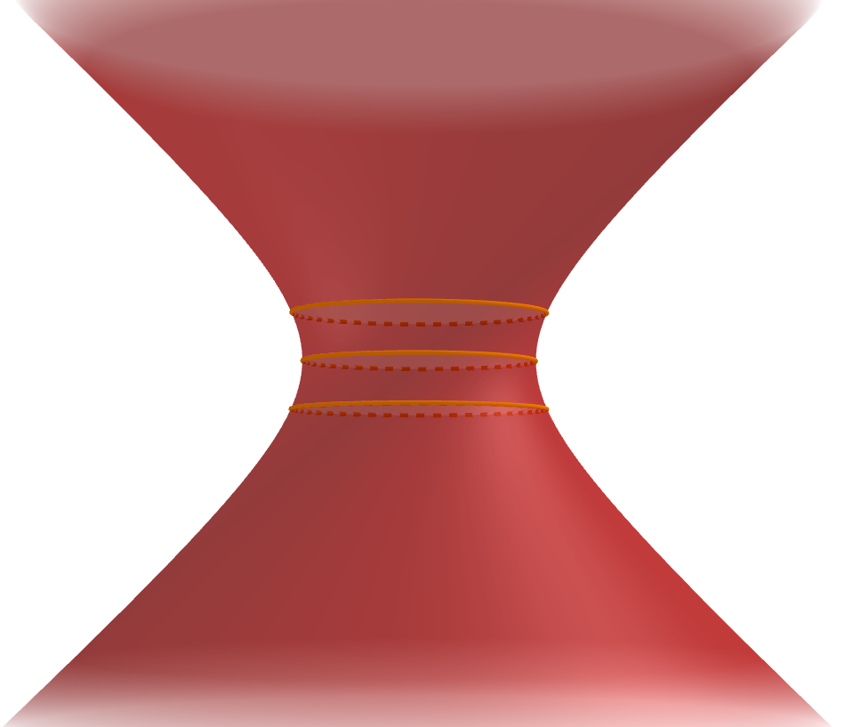
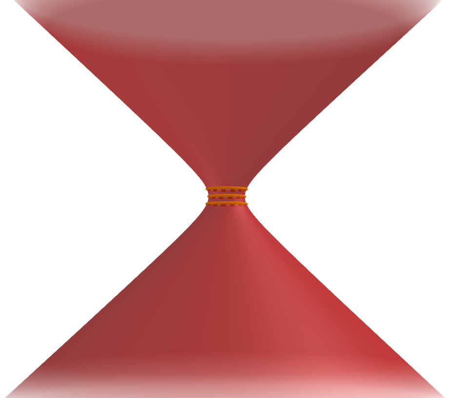
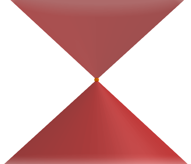
Figure 2. Rescaling to the nilcone

The operators $\mathrm{Op}_{\operatorname{h}}(a)$ are negligible unless $a$ is supported near $\mathcal{N}$. We thereby obtain in the $\operatorname{h}\rightarrow 0$ limit a sequence

$$\{\text{functions $\mathcal{N}\rightarrow\mathbb{R}$}\}\xrightarrow{\mathrm{Op}_{\operatorname{h}}}\{\text{self-adjoint $T\in\operatorname{End}(\pi)$}\}\rightarrow\{\text{measures on $[G]$}\}$$ (1.18)

where the final map sends $T=\sum v_{i}\otimes\overline{v_{i}}\in\operatorname{End}(\pi)\cong\pi\otimes\overline{\pi}$ to $\sum|v_{i}|^{2}(x)\,dx$, with $dx$ the chosen Haar measure on $[G]$. In §8, we implement this informal discussion rigorously and construct a $G$-equivariant limit map from functions on $\mathcal{N}$ to measures on $[G]$. We emphasize that this limit map is insensitive to the shape of the unscaled coadjoint orbit $\mathcal{O}_{\pi}$, whose role becomes replaced in the limit by a subset of the nilcone $\mathcal{N}$.

A key observation is now that the limits of the measures on $[G]$ obtained via (1.18) may be understood using Ratner’s theorem. The application of Ratner is indirect, because these measures themselves do not acquire any obvious additional invariance; rather, they may be decomposed into measures having unipotent invariance.

Indeed, after suitably rescaling, we may describe the limiting behavior of the sequence (1.18) in terms of a $G$-invariant measure $\mu$ on the product space $\mathcal{N}\times[G]$. Let $\mathcal{N}_{{\mathrm{reg}}}\subseteq\mathcal{N}$ denote the regular subset; it is the union of the open $G$-orbits on the nilcone $\mathcal{N}$, and its complement $\mathcal{N}-\mathcal{N}_{{\mathrm{reg}}}$ has lower dimension. We assume that $\pi$ is generic, or equivalently, has maximal Gelfand–Kirillov dimension (cf. §11.4.2); for instance, the principal series satisfy this assumption. Then the support of $\mu$ intersects $\mathcal{N}_{{\mathrm{reg}}}\times[G]$. By disintegrating the restriction of $\mu$ to $\mathcal{N}_{{\mathrm{reg}}}\times[G]$ over the projection to $\mathcal{N}_{{\mathrm{reg}}}$, we obtain a nontrivial family of measures $\mu_{\xi}$ on $[G]$ indexed by $\xi\in\mathcal{N}_{{\mathrm{reg}}}$. Speaking informally, we may regard $\mu_{\xi}$ as the $\operatorname{h}\rightarrow 0$ limit of an average of $L^{2}$-masses $|v_{\xi}|^{2}(x)\,dx$ taken over all vectors $v_{\xi}$ microlocalized at $\xi$. In any case, each such measure $\mu_{\xi}$ is invariant by the centralizer of the regular nilpotent element $\xi$. In favorable situations, an application of Ratner’s theorem then forces the $\mu_{\xi}$ and hence $\mu$ itself to be uniform.

This last paragraph mimics, in the context of Lie group representations, some of the semiclassical ideas behind the construction of the microlocal lift. We discuss this connection at more length in a sequel to this paper.

The argument just described gives a rich supply of families $(v_{i})_{i\in I}$ of vectors $v_{i}\in\pi$ for which

$$\int_{[G]}|v_{i}|^{2}\Psi\sim\frac{\int_{[G]}|v_{i}|^{2}}{\mathrm{vol}([G])}\int_{[G]}\Psi\quad\text{ on average over $i\in I$}$$ (1.19)

for fixed continuous functions $\Psi$ on $[G]$. Although the characteristic function of $[H]\subseteq[G]$ is not itself continuous, we may deduce an averaged form of (1.9) by applying a similar argument to the derivatives of the functions obtained via (1.18) and appealing to the Sobolev lemma. This approach may be understood as an infinitesimal variant of the “period thickening” technique of Bernstein–Reznikov [BR1].

1.9. Branching and stability

Having indicated how we achieve the objective (1.9), we turn now to the problem of producing (families of) vectors $v$ which pick out the family $\mathcal{F}$ as in (1.8).

This is a quantitative version of the branching problem in representation theory: we wish to understand not only how a representation of $G$ restricts to $H$, but in fact the behavior of individual vectors under the restriction process. Our approach is inspired by the following basic principle of the orbit method: restricting $\pi$ to $H$ should correspond to

$$\mbox{disintegrating the coadjoint orbit $\mathcal{O}_{\pi}$ along the projection $\mathfrak{g}^{\wedge}\rightarrow\mathfrak{h}^{\wedge}$}.$$ (1.20)

For example, the distinction of $\sigma$ by $\pi$ should be equivalent, at least asymptotically, to the existence of a solution to the equation

$$\xi|_{\mathfrak{h}}=\eta$$ (1.21)

with $(\xi,\eta)\in\mathcal{O}_{\pi}\times\mathcal{O}_{\sigma}\subseteq\mathfrak{g}^{\wedge}\times\mathfrak{h}^{\wedge}$.

The geometry of the projection (1.20) plays an important role in our argument, so we devote a fair amount of space to studying it in a purely algebraic context (see §13, §14, §16). Of particular significance is the branch locus of (1.20), i.e., the locus where the map $\mathcal{O}_{\pi}\rightarrow\mathfrak{h}^{\wedge}$ induced by (1.20) fails to have surjective differential. Many features of our analysis break down near this branch locus.

We recall, from geometric invariant theory, that $\xi\in\mathfrak{g}^{\wedge}$ is called stable if the following conditions are satisfied (see §14 for details):

• $\xi$ does not lie in the branch locus; equivalently, $\xi$ has trivial $\mathfrak{h}$-stabilizer.

• $\xi$ has closed $\mathbf{H}$-orbit, where $\mathbf{H}$ is the algebraic group underlying $H$.

This notion plays a fundamental role in our paper, and appears to be analytically significant: the complement of the stable locus is where the analytic conductor $C(\pi\times\overline{\sigma})$ of the Rankin–Selberg $L$-function $L(\pi\times\overline{\sigma},s)$ drops (see §15.4).

For instance, in the basic examples depicted in Figure 1, with $G\in\{\mathrm{SO}(3),\mathrm{SO}(1,2)\}$ and $H=\mathrm{SO}(2)$, the coadjoint orbits for $H$ are just singletons $\{\eta\}$, corresponding to one-dimensional representations, and the equation (1.21) says that $\xi$ should have $z$-coordinate given by $\eta$; in other words, the solutions to (1.21) are the horizontal slices shown in the diagram.

The stable case, in Figure 1, is when $\xi$ is not at the north or south poles of the sphere. Note that the the group $H=\mathrm{SO}(2)$ of rotations fixing the $z$-axis acts transitively on any circle in $\mathcal{O}_{\pi}$ with $z$-coordinate $\eta$, and freely away from the poles. This is a general pattern: the set of solutions to (1.21) – if nonempty – admits a diagonal action by $H$, which is simply transitive in the stable case (cf. §14.3, §17).

Figure 3 depicts the coadjoint orbit of a principal series representation $\pi$ of $G=\mathrm{SO}(1,2)\cong\mathrm{PGL}_{2}(\mathbb{R})$, with $H$ the diagonal subgroup $\mathrm{SO}(1,1)\cong\operatorname{GL}_{1}(\mathbb{R})$.

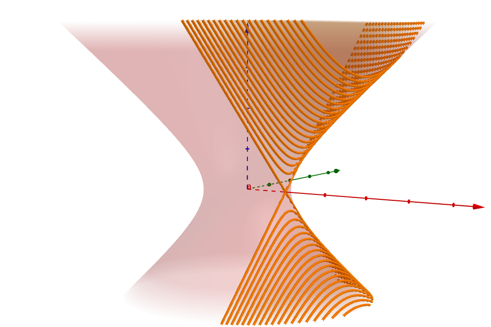
Figure 3. $H$-orbits on the one-sheeted hyperboloid

One sees again that $H$ acts simply transitively on generic fibers (i.e., away from the “cross”).

1.10. Analysis of matrix coefficient integrals; inverse branching

Having set up the necessary preliminaries regarding the geometry of orbits, we return to the problem of producing (families of) vectors $v$ which pick out the family $\mathcal{F}$ as in (1.8). The solution involves several steps which may be of independent interest:

1. We prove in §19 some asymptotic formulas for $\|\mathrm{pr}_{\sigma}(v)\|^{2}$, on average over $v$, when the pair $(\pi,\sigma)$ is tempered and the infinitesimal characters of $\pi$ and $\sigma$ satisfy a stability condition (see §14.2 for the exact definition). In more technical terms, we compute asymptotically the Fourier transform of relative characters in a small neighbourhood of the identity. The asymptotic formulae readily give a solution (§4) to the inverse problem of producing (families of) $v$ approximating a given function $\sigma\mapsto\|\mathrm{pr}_{\sigma}(v)\|^{2}$. The proofs depend heavily upon the operator calculus discussed in §1.7.

2. We must estimate the “undesirable” contributions to (1.5) coming from $\sigma$ which are either non-tempered, non-stable or of “high frequency.” The proofs (see, e.g., §4.3 and §11) apply the operator calculus. We refer to §10 for some discussion of the relevant subtleties.

As illustration, let us indicate how the methods underlying steps (i) and (ii) address the analytic test vector problem for a tempered pair $(\pi,\sigma)$ in the stable case, i.e., away from conductor-dropping. Informally speaking, that problem is to find

“nice” vectors $$v\in\pi u\in\sigma |\langle\mathrm{pr}_{\sigma}(v),u\rangle|^{2}$$ and for which the local period is “large”.

Solutions to this problem have appeared in period-based approaches to the subconvexity period (see, e.g., [MV, §3.6.1], [Nel3, §2.17.1], [BR2], [Rez], [DN], [Blo], [Nel2, Rmk 50], [HNS, Thm 1.2]); the point is that the period formula (1.7) and a “trivial” estimate for the global period $\int_{[H]}v\overline{u}$ often suffice to recover the convexity bound for $L$-function, suggesting the possibility for improvement in arithmetic settings via Hecke amplification.

The problem reduces to a robust understanding of the asymptotics of the local periods, which may be expressed in terms of matrix coefficient integrals as follows (see §18):

$$|\langle\mathrm{pr}_{\sigma}(v),u\rangle|^{2}=\int_{s\in H}\langle\pi(s)v,v\rangle\langle u,\sigma(s)u\rangle.$$ (1.22)

Such integrals had previously been estimated in some low-rank examples (see, e.g., [Wat, Wo, BR2, NPS, MS1, FS]) via explicit calculation.

To analyze (1.22), first decompose as in §1.7 to reduce to the case that $v$ and $u$ are microlocalized at some elements $\xi\in\operatorname{h}\mathcal{O}_{\pi}$ and $\eta\in\operatorname{h}\mathcal{O}_{\sigma}$ of the rescaled coadjoint orbits. If $\xi,\eta$ do not satisfy (1.21), at least up to some small error, then the resulting integral is readily seen to be negligible.

We thereby reduce to giving an asymptotic expansion for (1.22) when $v$ and $u$ are microlocalized at a stable solution $(\xi,\eta)$ to (1.21). One of the main local results of this paper (§19) establishes such expansions after averaging over small families of microlocalized vectors, of cardinality $\operatorname{O}(\operatorname{h}^{-\varepsilon})$ for any fixed $\varepsilon>0$ . Such averages are harmless for the applications pursued here; we note that the basic technique applies also in $p$-adic settings, where such averages may often be omitted (see [HNS, §3] for illustration in a basic example). Our expansions give in particular a solution to the test vector problem (modulo taking small averages), which appears to be new even in some low-rank cases (e.g., for discrete series representations in the triple product setting $H=\operatorname{GL}_{2}(\mathbb{R})\leqslant G=\operatorname{GL}_{2}(\mathbb{R})^{2}$).

We summarize the proof of the local result just described. The stability hypothesis ensures that if a group element $s\in H$ is not too close to the identity, then it moves any solution to (1.21) a fair bit (cf. §19.7 for details), so the microlocal support of the pair of vectors $\pi(s)v$ and $\sigma(s)v$ is disjoint from that of $v$ and $u$, and so the matrix coefficient integrand in (1.22) is negligible. We may thus truncate the integral (1.22) to the range where $s$ is small. We evaluate the contribution from this range asymptotically (§19.5), after a small average over $v$ and $u$, by applying the Kirillov formula for $\pi$ and $\sigma$. The application involves some pleasant book-keeping (§16, §17) concerning disintegration of volume forms (e.g., of $d\omega$ on $\mathcal{O}_{\pi}$ under $\mathcal{O}_{\pi}\rightarrow\mathfrak{h}^{\wedge}/\mkern-6.0mu/H$).

The methods described here are more than adequate to produce families of $v$ which pick out the fairly coarse families $\mathcal{F}$ required by our motivating application; see §4. We hope that they will be useful in many other problems involving asymptotic analysis of special functions arising from representations of higher rank groups. There are several avenues for extending our methods further. For instance, it seems to us an intriguing problem to obtain analogous asymptotic expansions in non-stable cases.

1.11. Comparison with other work

We briefly discuss the relationship of the ideas of this paper to some others:

1. The general philosophy that equidistribution results lead to mean value theorems for $L$-functions was advocated in [Ve], but the source of the equidistribution in this paper is quite different from that in [Ve]. The latter dealt exclusively with translates of a given vector by a large group element, which do not pick out sufficiently flexible families to be useful for the higher-rank applications pursued here.

2. Bernstein and Reznikov initiated the systematic application of identities such as (1.7), with a carefully chosen vector, to the problem of estimating branching coefficients (on average or individually). Their ideas have significantly influenced our basic strategy, as described in §1.6.

3. The orbit method [Kir2] is very well-known in the representation theory of Lie groups and widely used in the algebraic side of that theory. It is particularly satisfactory in the nilpotent case [Kir1, ShTs]. However it does not seem to have been used much in the way of this paper – that is to say, developed quantitatively along the lines of microlocal analysis and used as an analytical tool. One example where it has been applied in such a context is the asymptotic analysis of Wigner $6j$ symbols; see [Rob]. We hope it will be useful in many other contexts like this.

Although we have focused on applications to the averaged Gan–Gross–Prasad period, we hope that the ideas and methods of this paper, especially those related to the orbit method, should be helpful in a broader class of problems involving analysis of automorphic forms in higher rank.

1.12. Reading suggestions

The reader might wish to peruse Part I and then to skip directly to Part V, referring back to earlier results as needed.

1.13. Acknowledgments

We would like to thank Joseph Bernstein, Philippe Michel, and Andre Reznikov for many inspiring discussions, Emmanuel Kowalski for helpful feedback on an earlier draft, Davide Matasci for some corrections and the anonymous referee for a thorough reading and many helpful suggestions that have improved this paper.

During the completion of this paper, A.V. was an Infosys member at the Institute for Advanced Study. He would like to thank the IAS for providing wonderful working conditions. Over the course of writing the paper he received support from the Packard foundation and the National Science Foundation.

Parts of this work were carried out during visits of P.N. to Stanford in 2013–2016, at a 2014 summer school at the Institut des Hautes Études Scientifiques, while in residence in Spring 2017 at the Mathematical Sciences Research Institute, and during a couple short-term visits in Spring 2018 to the Institute for Advanced Study. He thanks all of these institutions for their support and excellent working conditions.

1.14. General notation and conventions

We collect these here together for the reader’s convenience. We have attempted to include reminders where appropriate throughout the text.

1.14.1. Asymptotic notation

We write $X=\operatorname{O}(Y)$ or $X\ll Y$ or $Y\gg X$ to denote that $|X|\leqslant c|Y|$ for some quantity $c$ which is “constant” or “fixed”, with precise meanings clarified in each situation. We write $X\asymp Y$ to denote that $X\ll Y\ll X$. “Implied constants” are allowed to depend freely upon any local fields, groups, norms, or bases under consideration.

1.14.2. The asymptotic parameter $\operatorname{h}$

Throughout this paper, the symbol $\operatorname{h}$ will denote a parameter in $(0,1]$. Whenever we use this notation, there will always be an implicit subset $\mathcal{H}\subseteq(0,1]$ in which the parameter $\operatorname{h}$ takes values; this subset will usually (but not always) be a discrete set with $0$ as its only limit point, reflecting, e.g., the wavelength scale of a family of Laplace eigenfunctions.

We always require the implied constants in any asymptotic notation to be independent of $\operatorname{h}$. We use notation such as $\operatorname{O}(\operatorname{h}^{\infty})$ to denote a quantity of the form $\operatorname{O}(\operatorname{h}^{N})$ for any fixed $N$.

By an “$\operatorname{h}$-dependent element” $s$ of some set $S$, we mean an element that depends, perhaps implicitly, upon the parameter $\operatorname{h}\in\mathcal{H}$, thus $s=s(\operatorname{h})$. We might understand $s$ more formally as an assignment $\mathcal{H}\rightarrow S$, $\operatorname{h}\mapsto s(\operatorname{h})$. For instance, an $\operatorname{h}$-dependent positive real $c=c(\operatorname{h})\in\mathbb{R}^{\times}_{+}$ is a map $\mathcal{H}\rightarrow\mathbb{R}^{\times}_{+}$. The parameter $\operatorname{h}$ itself may be understood as an $\operatorname{h}$-dependent positive real, corresponding to the identity map. The terminology applies even if the set itself varies with $\operatorname{h}$, thus $S=S(\operatorname{h})$; an $\operatorname{h}$-dependent element of $S$ is then an element of the Cartesian product $\prod_{\operatorname{h}}S(\operatorname{h})$.

1.14.3. Translating between $\operatorname{h}$-dependent and absolute formulations

The results stated in this paper in terms of $\operatorname{h}$-dependent elements can often be reformulated quantitatively for individual $\operatorname{h}$. Namely, a theorem formulated in terms of an arbitrary $\operatorname{h}$-dependent sequence $\pi_{\operatorname{h}}$ is formally equivalent to an “absolute” statement valid for all $\pi$ and all $\operatorname{h}\in(0,1)$. More frequently, we encounter theorems involving an arbitrary $\operatorname{h}$-dependent sequence $\pi_{\operatorname{h}}$ and an $\operatorname{h}$-dependent sequence $f_{\operatorname{h}}$ of functions which remain bounded with respect to certain norms, where the norms themselves are typically $\operatorname{h}$-dependent. Such theorems may likewise be reformulated as quantitative bounds valid for all $\pi,f$ and $\operatorname{h}\in(0,1)$. We illustrate this translation in Remark 1 of §6.3. As one sees in this example, the resulting absolute statements are more explicit but less succinct. For this reason, we have usually preferred the $\operatorname{h}$-dependent formulation in this paper.

1.14.4. Groups

Let $k$ be a field of characteristic zero. We denote by $\overline{k}$ an algebraic closure of $k$.

We generally denote by $X$ the set of $k$-points of a $k$-variety $\mathbf{X}$ (and vice-versa, if $\mathbf{X}$ is clear by context). We identify $\mathbf{X}$ with $X$ when $k=\overline{k}$.

By a reductive group $\mathbf{G}$ over $k$, we will always mean a connected reductive algebraic $k$-group $\mathbf{G}$. The set $G$ of $k$-points of $\mathbf{G}$ is then Zariski dense (see [Bor3, Corollary 18.3]).

We will frequently use restriction of scalars to regard reductive groups over $\mathbb{C}$ also as reductive groups over $\mathbb{R}$.

For an algebraic $k$-group $\mathbf{G}$, we denote by $G$, $\mathfrak{g}$ and $\mathfrak{g}^{*}$ the respective sets of $k$-points of $\mathbf{G}$, of its Lie algebra, and of the $k$-dual of its Lie algebra. The group $G$ acts on $\mathfrak{g}$ and $\mathfrak{g}^{*}$. Recall that an element of one of the latter spaces is regular if its orbit has maximal dimension, or equivalently, if its centralizer has minimal dimension. We use a subscripted “${\mathrm{reg}}$” to denote subsets of regular elements.

Suppose now that $\mathbf{G}$ is an algebraic group over an archimedean local field $F$, thus $F=\mathbb{R}$ or $\mathbb{C}$. We may then regard $G$ as a real Lie group; complex Lie groups do not play a role in this paper.

For a Lie group $G$, we write $\mathfrak{g}$ for its Lie algebra and $\mathfrak{g}^{\wedge}$ for the Pontryagin dual of $\mathfrak{g}$. We identify $\mathfrak{g}^{\wedge}$ with $i\mathfrak{g}^{*}$ (see §2.1 for details).

1.14.5. Unitary representations

Let $\mathbf{G}$ be a reductive group over a local field $k$ of characteristic zero. As above, we denote by $G$ the group of $k$-points of $\mathbf{G}$. By definition, a unitary representation $\pi$ of $G$ is a Hilbert space $V$ equipped with a strongly continuous homomorphism $\pi$ from $G$ to the group of unitary operators on $V$. In Part I, Part II and Appendix A, we commit the standard abuse of notation by writing $\pi$ for the Hilbert space $V$; we then denote by $\pi^{\infty}$ the subspace of smooth vectors (where in the non-archimedean case, “smooth” means “open stabilizer”). In §18, §19, Part IV and Part V, it will be convenient instead to write $\pi$ for the subspace of smooth vectors in $V$. It will occasionally be useful also to confuse “unitary” with “unitarizable.” The reader will be reminded locally of these conventions.

1.14.6. Topologies on vector spaces

When given a vector space $V$ defined as the subset of some larger space $\tilde{V}$ on which some $[0,+\infty]$-valued seminorms take finite values, we define $I(V)$ to be the set of restrictions to $V$ of those seminorms, and equip $V$ with its evident topology: that for which an open base at $v_{0}\in V$ is given by the sets $\{v\in V:\|v-v_{0}\|_{i}<\varepsilon\text{ for all }i\in M\}$, where $\varepsilon$ runs over the positive reals and $M$ over the finite subsets of $I(V)$. In all examples we consider, the seminorms will separate points, so $V$ will be a Hausdorff locally convex space.

Example 1.

This discussion applies to $V=C^{\infty}(U)$, for $U$ an open subset of $\mathbb{R}^{n}$, taking for $I(V)$ the set of pairs $(K,D)$, where $K\subseteq U$ is compact and $D$ is a differential operator (with smooth coefficients, say) on $\mathbb{R}^{n}$, with $\|f\|_{(K,D)}:=\sup_{x\in K}|Df(x)|$. It applies also to the Sobolev spaces $\pi^{s}$ ($s\in\mathbb{Z}\cup\{\infty\}$) defined below (§3.2) for a unitary representation $\pi$ of a Lie group.

Unwinding the definitions, a linear map $T:V\rightarrow W$ between two spaces so-equipped is continuous if for each $j\in I(W)$ there is a finite subset $M\subseteq I(V)$ and a scalar $C\geqslant 0$ so that

$$\|Tv\|_{j}\leqslant C\sum_{i\in M}\|v\|_{i}\text{ for all }v\in V,$$ (1.23)

while a family of such linear maps $T_{\alpha}:V\rightarrow W$ is equicontinuous if for each $j$, we may choose $M$ and $C$ uniformly with respect to the family’s indexing parameter $\alpha$. We might also describe the latter situation by saying that $T_{\alpha}$ is continuous, uniformly in $\alpha$.

We can make an analogous definition even if the spaces themselves vary, provided that the indexing sets for their seminorms admit natural identifications. Thus, suppose $T_{\alpha}:V_{\alpha}\rightarrow W_{\alpha}$ is a family of linear maps between spaces as above, and suppose also given identifications $I(V_{\alpha})=I(V_{\beta})$ and $I(W_{\alpha})=I(W_{\beta})$ for all $\alpha,\beta$. We may then speak as above of $T_{\alpha}$ being continuous, uniformly in $\alpha$.

Example 2.

Fix a Lie group $G$ and an element $x$ of its Lie algebra. As $\pi$ varies over the unitary representations of $G$, the family of operators $\pi^{\infty}\rightarrow\pi^{\infty}$ defined by $x$ is continuous, uniformly in $\pi$.

Let $V$ be a vector space arising as the increasing union of a sequence of topological vector subspaces $V_{m}$ as above, with continuous inclusions.

Example 3.

$C_{c}^{\infty}(U)$, for $U$ as in Example 1, can be described in this way, as can the space $\pi^{-\infty}=\cup_{s\in\mathbb{Z}}\pi^{s}$ of distributional vectors defined below (§3.2).

By the evident topology on $V$, we then mean the “locally convex inductive limit” topology, which may be characterized in either of the following ways:

1. It is the finest for which the inclusions $V_{m}\hookrightarrow V$ are continuous.

2. For every locally convex space $T$, the continuous maps $V\rightarrow T$ are precisely those that restrict to continuous maps $V_{m}\rightarrow T$ for each $m$.

Given another space $W$ as above, we say that a family of maps $T_{\alpha}:V\rightarrow W$ is continuous, uniformly in $\alpha$ if for each $m$, the family of restrictions $T_{\alpha}:V_{m}\rightarrow W$ has the property explained above.

We consider several examples (§4.5, §5.4, §12.1) of vector spaces $V$ consisting of “$\operatorname{h}$-dependent vectors in a varying family of vector spaces, equipped with the evident topology.” More formally, suppose given:

• $\operatorname{h}$-dependent vector spaces $V(\operatorname{h})$;

• An indexing set $\mathcal{I}$ for $\operatorname{h}$-dependent seminorms on $V(\operatorname{h})$; thus, for each $i\in\mathcal{I}$, we are given an $\operatorname{h}$-dependent seminorm $i(\operatorname{h}):V(\operatorname{h})\rightarrow[0,\infty]$.

Let $V$ denote the subspace of the Cartesian product $\prod_{\operatorname{h}}V(\operatorname{h})$ consisting of $\operatorname{h}$-dependent vectors $v=v(\operatorname{h})$ for which the seminorm

$$\|v\|_{V,i}:=\sup_{\operatorname{h}}\|v(\operatorname{h})\|_{i(\operatorname{h})}$$ (1.24)

is finite for each $i\in\mathcal{I}$. We then topologize $V$ by means of these seminorms.

Still in the situation just described, suppose given an $\operatorname{h}$-dependent positive real $c>0$. We denote by $cV$ the image of $V\subseteq\prod_{\operatorname{h}}V(\operatorname{h})$ under the bijection $v\mapsto cv=c(\operatorname{h})v(\operatorname{h})$, equipped with the seminorms and topology transported from $V$ via this bijection. Thus an $\operatorname{h}$-dependent vector $v=v(\operatorname{h})\in V(\operatorname{h})$ belongs to $cv$ if every seminorm

$$\|v\|_{cV,i}:=\sup_{\operatorname{h}\in(0,1]}\|c(\operatorname{h})^{-1}v(\operatorname{h})\|_{i(\operatorname{h})}$$

is finite. For instance, we may speak of the space $\operatorname{h}^{10}V$; it is the image of $V$ under multiplication by $\operatorname{h}^{10}$. We denote by $\operatorname{h}^{\infty}V$ the intersection $\cap_{\eta}\operatorname{h}^{\eta}V$, topologized in the evident way. In practice, $\operatorname{h}^{\infty}V$ consists of $\operatorname{h}$-dependent vectors which are “negligible” in the $\operatorname{h}\rightarrow 0$ limit.

Example 4.

Let $V$ be a finite-dimensional real vector space. We topologize the Schwartz space $\mathcal{S}(V)$, as usual, by means of the seminorms $f\mapsto\|Df\|_{L^{\infty}}$ indexed by the polynomial-coefficient differential operators $D$ on $V$. Per the above conventions, $\operatorname{h}^{\eta}\mathcal{S}(V)$ is the space of $\operatorname{h}$-dependent Schwartz functions $f=f(\operatorname{h})$ whose seminorms satisfy, for each $D$ as above,

$$\sup_{\operatorname{h}}\operatorname{h}^{-\eta}\|Df(\operatorname{h})\|_{L^{\infty}}<\infty.$$

We apply this notation even when $\eta=0$; elements of $\operatorname{h}^{0}\mathcal{S}(V)$ are then $\operatorname{h}$-dependent Schwartz functions whose seminorms are bounded uniformly with respect to $\operatorname{h}$.

1.14.7. Miscellaneous

For an element $\xi$ of a normed space, we often write

$$\langle\xi\rangle:=(1+|\xi|^{2})^{1/2}.$$

This quantifies the size of $\xi$, but is never smaller than $1$.

When we have equipped some space $X$ (e.g., a group $G$ as above) with a “standard” measure $\mu$ (e.g., a Haar measure), we often write $\int_{x\in X}f(x)$ as shorthand for the integral $\int_{x\in X}f(x)\,d\mu(x)$ taken with respect to the standard measure.

We extend addition to a binary operation $+$ on the extended real line $\mathbb{R}\cup\{\pm\infty\}$, given by

$$\infty+(-\infty)=(-\infty)+\infty:=-\infty,$$

and in other cases in the obvious way; this extension is used starting in §4.5.

Part I Microlocal analysis on Lie group representations I: definitions and basic properties

Let $G$ be a unimodular Lie group over $\mathbb{R}$, with Lie algebra $\mathfrak{g}$. Let $\pi$ be a unitary representation of $G$. This part (Part I) and its sequel (Part II) will study the basic quantitative properties of an assignment $\mathrm{Op}$ from functions on the dual of $\mathfrak{g}$ to operators on $\pi$. We will describe the contents of both parts here; we suggest that the reader peruse Part I and consult Part II as needed.

§2–§5 and their sequels §7–§8 concern aspects of this assignment which apply to any unitary representation $\pi$, such as $\pi=L^{2}(G)$. Their results may be equivalently formulated in terms of the convolution structure on $L^{1}(G)$, and more generally on spaces of distributions supported near and singular only at the identity element. In particular, all estimates in these sections are uniform in $\pi$.

In §9, we record some preliminaries concerning the relationship between representations of real reductive groups and their infinitesimal characters. These are relevant for us because our main result concerns averages over automorphic representations having infinitesimal character in a prescribed region.

§6 and its sequel §12 establish finer properties of $\mathrm{Op}$ for $G$ reductive and $\pi$ irreducible and tempered. The relevant consequence of these assumptions is the Kirillov-type formula.

We note that §19 of Part III applies the results of Part I to determine (under certain assumptions) the “asymptotic decomposition” of $\mathrm{Op}$ under restriction to certain subgroups.

The contents of Part I may be understood as generalizations of standard results in the theory of pseudodifferential operators (see [Hör, Be1] and references), which corresponds roughly to the case in which $G$ is $2$-step nilpotent. We note some minor differences:

1. The exponential map is neither injective nor surjective for the groups $G$ of interest to us, so we work within a fixed small enough neighborhood of the identity element of $G$.

2. The Baker–Campbell–Hausdorff formula is much simpler when $G$ is $2$-step nilpotent; for the $G$ of interest, it contains arbitrarily nested commutators. It was not obvious to us at the outset whether this would present an obstruction.

3. The appropriate way to generalize the standard operator classes in the theory of pseudodifferential operators was not obvious to us; the definition given in §3 took some work to identify.

We note that the $\star$-product implicit in our operator calculus on the Lie algebra has been previously considered by Rieffel [Ri], who observed that it gives a deformation quantization of the Poisson structure. As Rieffel observes in [Ri, p658]: “At the heuristic level, our results also mesh nicely with Kirillov’s orbit method for the theory of group representations, and perhaps the connection can be made stronger.” The results of this paper concerning the operator calculi may be seen as steps in this direction. We mention also the work of B. Cahen and B. Harris (see for instance [Cah, Har1]).

Notation

We denote by $\pi^{\infty}\leqslant\pi$ the (dense) subspace of smooth vectors, by $\mathfrak{U}$ the universal enveloping algebra of $\mathfrak{g}_{\mathbb{C}}$, and by $\pi:\mathfrak{U}\rightarrow\operatorname{End}(\pi^{\infty})$ the induced map. For $u\in\mathfrak{U}$, we occasionally write simply $u$ instead of $\pi(u)$ when it is clear from context that $u$ is acting on $\pi$.

2. Operators attached to Schwartz functions

We define here the basic construct of the microlocal calculus on representations: an assignment from Schwartz functions on the dual of the Lie algebra to operators. See (1.14) and surrounding discussion for motivation. We extend and refine this assignment in later sections.

2.1. Measures, Fourier transforms, etc.

We fix an open neighborhood $\mathcal{G}$ of the origin in the Lie algebra $\mathfrak{g}$, taken sufficiently small. In particular, $\exp:\mathcal{G}\rightarrow G$ is an analytic isomorphism onto its image.

We choose Haar measures $dg$ on $G$ and $dx$ on $\mathfrak{g}$ satisfying the following compatibility: for $x\in\mathcal{G}$ and $g=\exp(x)$, we have $dg=j(x)\,dx$, where the analytic function $j:\mathcal{G}\rightarrow\mathbb{R}_{>0}$ satisfies $j(0)=1$.

Since $\mathcal{G}$ is small, the image $j(\mathcal{G})$ is a precompact subset of $\mathbb{R}_{>0}$. We assume also that $-x\in\mathcal{G}$ whenever $x\in\mathcal{G}$.

We use the letters $x,y,z$ for elements of $\mathfrak{g}$ and $\xi,\eta,\zeta$ for elements of its imaginary dual $i\mathfrak{g}^{*}:=\operatorname{Hom}_{\mathbb{R}}(\mathfrak{g},i\mathbb{R})$. We denote the natural pairing by $x\xi:=\xi x:=\xi(x)\in i\mathbb{R}$.

Recall that $\mathfrak{g}^{\wedge}=\operatorname{Hom}(\mathfrak{g},\mathbb{C}^{(1)})$ denotes the Pontryagin dual. We identify $i\mathfrak{g}^{*}$ with $\mathfrak{g}^{\wedge}$ via the canonical isomorphism $\xi\mapsto[x\mapsto e^{x\xi}]$; we will find it clearer to work with $\mathfrak{g}^{\wedge}$ for analytic purposes, $i\mathfrak{g}^{*}$ for algebraic purposes. In particular, we identify $\mathfrak{g}$ with the space of $i\mathbb{R}$-valued linear functions on $\mathfrak{g}^{\wedge}$.

We write $\mathcal{S}(\dotsb)$ for the Schwartz space. We equip $\mathfrak{g}^{\wedge}$ with the Haar measure $d\xi$ for which the Fourier transforms $\mathcal{S}(\mathfrak{g})\ni\phi\mapsto\phi^{\wedge}\in\mathcal{S}(\mathfrak{g}^{\wedge})$ and $\mathcal{S}(\mathfrak{g}^{\wedge})\ni a\mapsto a^{\vee}\in\mathcal{S}(\mathfrak{g})$ defined by

$$\phi^{\wedge}(\xi):=\int_{x\in\mathfrak{g}}\phi(x)e^{x\xi}\,dx,\quad a^{\vee}(x):=\int_{\xi\in\mathfrak{g}^{\wedge}}a(\xi)e^{-x\xi}\,d\xi$$

are mutually inverse.

We let $G$ act on $\mathfrak{g}$ by the adjoint action $g\cdot x:=\mathrm{Ad}(g)x$, on $\mathfrak{g}^{\wedge}=i\mathfrak{g}^{*}$ by the coadjoint action $x(g\cdot\xi):=(g^{-1}\cdot x)\xi$, and on functions $f$ on either space by $g\cdot f:=f(g^{-1}\cdot-)$.

2.2. The basic operator map

For a neighborhood $\mathcal{G}$ of the origin in $\mathfrak{g}$ as above, we let $\mathcal{X}(\mathcal{G})$ denote the set of all “cutoffs” $\chi\in C_{c}^{\infty}(\mathcal{G})$ with the following properties:

1. $\chi$ is even: $\chi(x)=\chi(-x)$ for all $x$.

2. $\chi(x)\in[0,1]$ for all $x$. In particular, $\chi$ is real-valued.

3. $\chi(x)=1$ for all $x$ in some neighborhood of the origin.

For $\mathcal{G}$ as above, $\chi\in\mathcal{X}(\mathcal{G})$ and $a\in\mathcal{S}(\mathfrak{g}^{\wedge})$, we define the bounded operator $\mathrm{Op}(a,\chi:\pi)\in\operatorname{End}(\pi)$ by the formula

$$\mathrm{Op}(a,\chi:\pi)v:=\int_{x\in\mathfrak{g}}\chi(x)a^{\vee}(x)\pi(\exp(x))v\,dx.$$ (2.1)

We abbreviate $\mathrm{Op}(a,\chi):=\mathrm{Op}(a,\chi:\pi)$ when $\pi$ is clear from context. Starting in §5.4, we further abbreviate $\mathrm{Op}(a):=\mathrm{Op}(a,\chi)$.

Recall that $\operatorname{h}$ denotes a parameter in $(0,1]$. For $a$ as above, we define the rescaled function $a_{\operatorname{h}}(\xi):=a(\operatorname{h}\xi)$ and the correspondingly rescaled operator

$$\mathrm{Op}_{\operatorname{h}}(a,\chi):=\mathrm{Op}(a_{\operatorname{h}},\chi)=\int_{x\in\mathfrak{g}}\chi(\operatorname{h}x)a^{\vee}(x)\pi(\exp(\operatorname{h}x))\,dx.$$ (2.2)

As informal motivation for this definition, recall from (1.15) the desiderata that $\mathrm{Op}_{\operatorname{h}}(a)v\approx a(\xi)v$ for $v\in\pi$ microlocalized at $\xi\in\mathfrak{g}^{\wedge}$, i.e., for which $\pi(\exp(\operatorname{h}x))v\approx e^{x\xi}v$ whenever $|x|\ll 1$. Indeed, since $a^{\vee}(x)$ is small unless $|x|\ll 1$, in which case $\chi(\operatorname{h}x)=1$, we see from (2.2) that $\mathrm{Op}_{\operatorname{h}}(a,\chi)v\approx(\int_{x\in\mathfrak{g}}a^{\vee}(x)e^{x\xi}\,dx)v=a(\xi)v$.

2.3. Adjoints

Our assumptions on $\chi$ imply that the adjoint $\mathrm{Op}(a,\chi)^{*}$ of $\mathrm{Op}(a,\chi)$, regarded as a bounded operator on $\pi$, is given by $\mathrm{Op}(\overline{a},\chi)$.

2.4. Equivariance

Let $a\in\mathcal{S}(\mathfrak{g}^{\wedge})$, $g\in G$, $\chi\in\mathcal{X}(\mathcal{G})$. Assume that $\mathrm{Ad}(g){\mathrm{supp}}(\chi)\subseteq\mathcal{G}$. Then $g\cdot\chi\in\mathcal{X}(\mathcal{G})$, and we verify readily that $\pi(g)\mathrm{Op}(a,\chi)\pi(g)^{-1}=\mathrm{Op}(g\cdot a,g\cdot\chi)$.

2.5. Composition: preliminary discussion

For $f\in C_{c}^{\infty}(G)$, we define $\pi(f)\in\operatorname{End}(\pi)$ by $\pi(f)v:=\int_{g\in G}f(g)\pi(g)v\,dg$. Then

$$\pi(f_{1})\pi(f_{2})=\pi(f_{1}\ast f_{2}),$$ (2.3)

where $\ast$ denotes convolution. This fact unwinds to a composition formula for $\mathrm{Op}(a,\chi)$:

Suppose given a pair of open neighborhoods $\mathcal{G},\mathcal{G}^{\prime}$ of the origin as above and cutoffs $\chi\in\mathcal{X}(\mathcal{G}),\chi^{\prime}\in\mathcal{X}(\mathcal{G}^{\prime})$ for which:

1. $\exp(\mathcal{G})\exp(\mathcal{G})\subseteq\exp(\mathcal{G}^{\prime})$, so that we may define $\ast:\mathcal{G}\times\mathcal{G}\rightarrow\mathcal{G}^{\prime}$ by

   $$x\ast y:=\log(\exp(x)\exp(y)).$$

2. $\chi^{\prime}(x\ast y)=1$ for all $x,y\in{\mathrm{supp}}(\chi)$.

Let us denote temporarily by $\phi\mapsto f$ the topological isomorphism $C_{c}^{\infty}(\mathcal{G})\rightarrow C_{c}^{\infty}(\exp(\mathcal{G}))$ defined by the rule $f(\exp(x)):=\phi(x)j(x)^{-1}$. Then $f(g)\,dg$ is the pushforward of $\phi(x)\,dx$, and so $\pi(f)=\int_{x\in\mathfrak{g}}\phi(x)\pi(\exp(x))\,dx$. We may define continuous bilinear operators $\star$ on $C_{c}^{\infty}(\mathcal{G})$ and then on $\mathcal{S}(\mathfrak{g}^{\wedge})$ by requiring that the diagram

$$\begin{CD}C_{c}^{\infty}(\exp(\mathcal{G}))^{2}@>{\ast}>{}>C_{c}^{\infty}(\exp(\mathcal{G}^{\prime}))\\ @A{\cong}A{\phi\mapsto f}A@V{f\mapsto\phi}V{\cong}V\\ C_{c}^{\infty}(\mathcal{G})^{2}@>{\star}>{}>C_{c}^{\infty}(\mathcal{G}^{\prime})\\ @A{}A{a\mapsto\chi a^{\vee}}A@V{\phi\mapsto\phi^{\wedge}}V{}V\\ \mathcal{S}(\mathfrak{g}^{\wedge})^{2}@>{\star}>{}>\mathcal{S}(\mathfrak{g}^{\wedge})\end{CD}$$

commute. The top arrow is defined thanks to (i). The middle arrow may be described conveniently in terms of the Fourier transform: for $\phi_{1},\phi_{2}\in C_{c}^{\infty}(\mathcal{G})$ and $\zeta\in\mathfrak{g}^{\wedge}$,

$$\int_{z\in\mathfrak{g}}\phi_{1}\star\phi_{2}(z)e^{z\zeta}\,dz=\int_{x,y\in\mathfrak{g}}\phi_{1}(x)\phi_{2}(y)e^{(x\ast y)\zeta}\,dx\,dy.$$ (2.4)

(Indeed, by definition, $\phi_{1}\star\phi_{2}(z)\,dz$ is obtained from $\phi_{1}(x)\phi_{2}(y)\,dx\,dy$ by pushing forward to the group, convolving, and then pulling back to the Lie algebra; testing this definition against $z\mapsto e^{z\zeta}$ gives (2.4).) The bottom arrow, which we refer to as the star product, is given by $a_{1}\star a_{2}=(\chi a_{1}^{\vee}\star\chi a_{2}^{\vee})^{\wedge}$. Note that $\star$ depends upon $\chi$.

Lemma.

For $a_{1},a_{2}\in\mathcal{S}(\mathfrak{g}^{\wedge})$,

$$\mathrm{Op}(a_{1},\chi)\mathrm{Op}(a_{2},\chi)=\mathrm{Op}(a_{1}\star a_{2},\chi^{\prime}).$$ (2.5)

Proof.

Set $\phi_{i}:=\chi a_{i}^{\vee}\in C_{c}^{\infty}(\mathcal{G})$, and let $f_{i}\in C_{c}^{\infty}(\exp(\mathcal{G}))$ be as associated above. The identity (2.5) follows from (2.3) upon unwinding the definitions and noting that $\chi^{\prime}\equiv 1$ on the support of $\chi a_{1}^{\vee}\star\chi a_{2}^{\vee}$. ∎

We also have the rescaled composition formula $\mathrm{Op}_{\operatorname{h}}(a,\chi)\mathrm{Op}_{\operatorname{h}}(b,\chi)=\mathrm{Op}(a\star_{\operatorname{h}}b,\chi^{\prime})$, where the rescaled star product $a\star_{\operatorname{h}}b$ is defined by requiring that

$$(a\star_{\operatorname{h}}b)_{\operatorname{h}}=a_{\operatorname{h}}\star b_{\operatorname{h}}.$$

We note that $\star$ is recovered from $\star_{\operatorname{h}}$ by taking $\operatorname{h}=1$.

3. Operator classes

The operator map (2.1) has been defined for functions $a$ belonging to the Schwartz space of $\mathfrak{g}^{\wedge}$. We want to extend it to other functions, e.g., functions $a$ that are permitted polynomial growth at $\infty$. In that case, $\mathrm{Op}(a)$ is no longer a bounded map $\pi\rightarrow\pi$; rather, it behaves more like the (densely defined) operator on $\pi$ induced by an element of the universal enveloping algebra.

Motivated by this, we define certain classes of densely defined operators on $\pi$. These classes will eventually serve as the target of $\mathrm{Op}$, after we extend its definition to various symbol classes.

3.1. The operator $\Delta$ and its inverse

Let us fix a basis $\mathcal{B}:=\mathcal{B}(\mathfrak{g})$ of $\mathfrak{g}$, and set

$$\Delta:=\Delta_{G}:=1-\sum_{x\in\mathcal{B}}x^{2}\in\mathfrak{U}.$$

We will often confuse $\Delta$ with its image $\pi(\Delta)\in\operatorname{End}(\pi^{\infty})$. It has the following properties:

1. It induces a densely-defined self-adjoint positive operator on $\pi$ with bounded inverse $\Delta^{-1}$ (see [NS]). The operator norm of $\Delta^{-1}$ is $\leqslant 1$.

2. For $n\geqslant 0$, let $D(\Delta^{n})\subseteq\pi$ denote the domain of the densely-defined self-adjoint operator extending $\pi(\Delta^{n})$. Then $\pi^{\infty}=\cap_{n\geqslant 0}D(\Delta^{n})$ (see [Nel1, Cor 9.3]). Consequently, $\Delta^{-1}$ acts on $\pi^{\infty}$.

3.2. Sobolev spaces

For $s\in\mathbb{Z}$, we define an inner product $\langle-,-\rangle_{\pi^{s}}$ on $\pi^{\infty}$ by the rule

$$\langle v_{1},v_{2}\rangle_{\pi^{s}}:=\langle\Delta^{s}v_{1},v_{2}\rangle.$$

We denote by $\pi^{s}$ the Hilbert space completion of $\pi^{\infty}$ with respect to the associated norm $\|v\|_{\pi^{s}}:=\langle v,v\rangle_{\pi^{s}}^{1/2}$. These norms increase with $s$, so up to natural identifications,

$$\pi^{\infty}=\cap\pi^{s}\leqslant\dotsb\leqslant\pi^{s+1}\leqslant\pi^{s}\leqslant\pi^{s-1}\leqslant\dotsb\leqslant\pi^{-\infty}:=\cup\pi^{s}.$$

These spaces come with evident topologies (§1.14.6).

The inner product on $\pi$ induces a duality between $\pi^{s}$ and $\pi^{-s}$.

We note that for each $s\in\mathbb{Z}_{\geqslant 0}$ there exist $C_{s}>c_{s}>0$, depending upon $\mathcal{B}$, so that

$$c_{s}\|v\|_{\pi^{s}}^{2}\leqslant\sum_{r=0}^{s}\sum_{x_{1},\dotsc,x_{r}\in\mathcal{B}}\|x_{1}\dotsb x_{r}v\|^{2}\leqslant C_{s}\|v\|_{\pi^{s}}^{2}$$ (3.1)

(see, e.g., [Nel1, proof of Lem 6.3]).

3.3. Definition of operator classes

By an operator on $\pi$, we mean simply a linear map $T:\pi^{\infty}\rightarrow\pi^{-\infty}$. For each $x\in\mathfrak{g}$, the commutator

$$\theta_{x}(T):=[\pi(x),T]$$

is likewise an operator on $\pi$. Indeed, by (3.1), we have for $s\geqslant 1$ that $\pi(x):\pi^{s}\rightarrow\pi^{s-1}$. By duality, it follows that $\pi(x):\pi^{1-s}\rightarrow\pi^{-s}$. In particular, $\pi(x)$ acts on both $\pi^{\infty}$ and $\pi^{-\infty}$, so both compositions $\pi(x)\circ T$ and $T\circ\pi(x)$ are defined.

The map $x\mapsto\theta_{x}$ extends to an algebra morphism $\mathfrak{U}\rightarrow\operatorname{End}(\{\text{operators on $\pi$}\})$, denoted $u\mapsto\theta_{u}$. For example, for $x_{1},\dotsc,x_{n}\in\mathfrak{g}$,

$$\theta_{x_{1}\dotsb x_{n}}(T)=[\pi(x_{1}),[\pi(x_{2}),\dotsc,[\pi(x_{n}),T]]].$$

Definition.

For $m\in\mathbb{Z}$, we say that an operator $T$ on $\pi$ has order $\leqslant m$ if for each $s\in\mathbb{Z}$ and $u\in\mathfrak{U}$, the operator $\theta_{u}(T)$ induces a bounded map

$$\theta_{u}(T):\pi^{s}\rightarrow\pi^{s-m}.$$

Remark.

When $\pi$ is a standard representation of a Heisenberg group, this definition is closely related to Beals’s characterization [Be2] of pseudodifferential operators.

We denote by $\Psi^{m}:=\Psi^{m}(\pi)$ the space of operators on $\pi$ of order $\leqslant m$, by $\Psi^{-\infty}:=\cap_{m}\Psi^{m}$ the space of “smoothing operators,” and by $\Psi^{\infty}:=\cup_{m}\Psi^{m}$ the space of “finite-order operators.” Then

$$\Psi^{-\infty}\subseteq\dotsb\subseteq\Psi^{m-1}\subseteq\Psi^{m}\subseteq\Psi^{m+1}\subseteq\dotsb\subseteq\Psi^{\infty}.$$ (3.2)

These spaces come with evident topologies (§1.14.6); thus for $m\in\mathbb{Z}$, the relevant seminorms on $\Psi^{m}$ are $T\mapsto\|\theta_{u}(T)\|_{\pi^{s}\rightarrow\pi^{s-m}}$, taken over $s\in\mathbb{Z}$ and $u\in\mathfrak{U}$. The inclusions (3.2) are continuous.

We note that $\Psi^{m}$ depends, implicitly, upon the group $G$ which we regard as acting on $\pi$.

3.4. Composition

Observe that finite-order operators act on the space of smooth vectors, i.e., $\Psi^{\infty}\subseteq\operatorname{End}(\pi^{\infty})$. We may thus compose such operators.

Lemma.

For $m_{1},m_{2}\in\mathbb{Z}\cup\{\pm\infty\}$, composition induces continuous maps $\Psi^{m_{1}}\times\Psi^{m_{2}}\rightarrow\Psi^{m_{1}+m_{2}}$, where as usual $\infty+(-\infty):=-\infty$.

Proof.

For $T_{1}\in\Psi^{m_{1}}$, $T_{2}\in\Psi^{m_{2}}$ and $u\in\mathfrak{U}$, we may write $\theta_{u}(T_{1}T_{2})$ as a sum of expressions $\theta_{u_{1}}(T_{1})\theta_{u_{2}}(T_{2})$ with $u_{1},u_{2}\in\mathfrak{U}$. For $s\in\mathbb{Z}$, the compositions of bounded maps

$$\pi^{s}\xrightarrow{\theta_{u_{2}}(T_{2})}\pi^{s-m_{2}}\xrightarrow{\theta_{u_{1}}(T_{1})}\pi^{s-m_{1}-m_{2}}$$

are bounded, and so $\theta_{u}(T_{1}T_{2})$ induces a bounded map $\pi^{s}\rightarrow\pi^{s-m_{1}-m_{2}}$, as required. ∎

3.5. Differential operators

It is easy to see that $\Psi^{0}$ contains the identity operator. We record some further examples:

Lemma.

Let $m\in\mathbb{Z}$. Then

• $\pi(\Delta)^{m}\in\Psi^{2m}$, and

• $\pi(x_{1}\dotsb x_{m})\in\Psi^{m}$ if $m\geqslant 0$ and $x_{1},\dotsc,x_{m}\in\mathfrak{g}$.

The proof is elementary but somewhat tedious, hence postponed to §8.5.

3.6. Smoothing operators

Lemma 1.

An operator $T$ on $\pi$ belongs to $\Psi^{-\infty}$ if and only if for each $N\in\mathbb{Z}_{\geqslant 0}$, the operator $\Delta^{N}T\Delta^{N}$ induces a bounded map $\pi\rightarrow\pi$. The corresponding seminorms $T\mapsto\|\Delta^{N}T\Delta^{N}\|_{\pi\rightarrow\pi}$ describe the topology on $\Psi^{-\infty}$.

Proof.

This follows readily from (3.1) and the definitions. ∎

Lemma 2.

For $f\in C_{c}^{\infty}(G)$, one has $\pi(f)\in\Psi^{-\infty}$, and the induced map

$$C_{c}^{\infty}(G)\rightarrow\Psi^{-\infty}$$

is continuous.

Proof.

Set $f^{\prime}:=\Delta^{N}\ast f\ast\Delta^{N}$. We note that $\Delta^{N}\pi(f)\Delta^{N}=\pi(f^{\prime})$, that $\|\pi(f^{\prime})\|_{\pi\rightarrow\pi}\leqslant\|f^{\prime}\|_{L^{1}}$, and that the map $f\mapsto f^{\prime}$ on $C_{c}^{\infty}(G)$ is continuous. ∎

4. Symbol classes

As promised, we now define various enlargements of the Schwartz space; we will later extend $\mathrm{Op}$ to these spaces.

We also study the behavior of the star products $\star$ and $\star_{\operatorname{h}}$, defined above, on these enlarged spaces. Eventually, under $\mathrm{Op}$, these products will be intertwined with operator composition.

4.1. Multi-index notation

Temporarily denote by $n:=\dim(G)$ the dimension of the underlying Lie group. For convenience, we choose a basis for $\mathfrak{g}$. This choice defines coordinates $\mathfrak{g}\ni x\mapsto(x_{1},\dotsc,x_{n})\in\mathbb{R}^{n}$ and $\mathfrak{g}^{\wedge}\ni\xi\mapsto(\xi_{1},\dotsc,\xi_{n})\in i\mathbb{R}^{n}$ for which $x\xi=x_{1}\xi_{1}+\dotsb+x_{n}\xi_{n}$.

For each “multi-index” $\alpha\in\mathbb{Z}_{\geqslant 0}^{n}$ we set $|\alpha|:=\alpha_{1}+\dotsb+\alpha_{n}$ and $\alpha!:=\alpha_{1}!\dotsb\alpha_{n}!$ and $x^{\alpha}:=x_{1}^{\alpha_{1}}\dotsb x_{n}^{\alpha_{n}}\in\mathbb{R}$ and $\xi^{\alpha}:=\xi_{1}^{\alpha_{1}}\dotsb\xi_{n}^{\alpha_{n}}\in i^{|\alpha|}\mathbb{R}$. We define the differential operators $\partial^{\alpha}$ on $C^{\infty}(\mathfrak{g}^{\wedge})$ and on $C^{\infty}(\mathfrak{g})$ by requiring that

$$(\partial^{\alpha}a)^{\vee}(x)=x^{\alpha}a^{\vee}(x),\quad(\partial^{\alpha}\phi)^{\wedge}(\xi)=(-\xi)^{\alpha}\phi^{\wedge}(\xi)$$ (4.1)

for $a\in C^{\infty}(\mathfrak{g}^{\wedge})$ and $\phi\in C^{\infty}(\mathfrak{g})$; the formal Taylor expansions then read

$$a(\zeta+\xi)=\sum_{\alpha}\frac{\xi^{\alpha}}{\alpha!}\partial^{\alpha}a(\zeta),\quad\phi(z+x)=\sum_{\alpha}\frac{x^{\alpha}}{\alpha!}\partial^{\alpha}\phi(z).$$

We fix norms $|.|$ on $\mathfrak{g}$ and $\mathfrak{g}^{\wedge}$. Recall that we abbreviate $\langle\xi\rangle:=(1+|\xi|^{2})^{1/2}$.

4.2. Formal expansion of the star product

Let $\ast$ and $\star_{h}$ be as in §2.5. We define the analytic map $\{\cdot,\cdot\}:\mathcal{G}\times\mathcal{G}\rightarrow\mathfrak{g}$ to be the “remainder term” $\{x,y\}:=x\ast y-x-y$ in the Baker–Campbell–Hausdorff formula. It follows then from (2.4) that for $a,b\in\mathcal{S}(\mathfrak{g}^{\wedge})$,

$$a\star b(\zeta)=\int_{x,y\in\mathfrak{g}}a^{\vee}(x)b^{\vee}(y)e^{x\zeta}e^{y\zeta}e^{\{x,y\}\zeta}\chi(x)\chi(y)\,dx\,dy.$$ (4.2)

The factor $e^{\{x,y\}\zeta}\in\mathbb{C}^{(1)}$ defines an analytic function of $(x,y,\zeta)\in\mathcal{G}\times\mathcal{G}\times\mathfrak{g}^{\wedge}$, and so admits a power series expansion

$$e^{\{x,y\}\zeta}=\sum_{\alpha,\beta,\gamma}c_{\alpha\beta\gamma}x^{\alpha}y^{\beta}\zeta^{\gamma}.$$ (4.3)

The estimate $\{x,y\}=\operatorname{O}(|x|\,|y|)$ controls which monomials $x^{\alpha}y^{\beta}\zeta^{\gamma}$ actually appear in this expansion. Using superscript to indicate degree, the terms appearing are $1$, then $x^{r}y^{s}\zeta^{1}(r,s\geqslant 1)$, then $x^{r}y^{s}\zeta^{2}(r,s\geqslant 2)$, and so on. In particular, $x^{a}y^{b}\zeta^{c}$ appears only if $j=a+b-c$ is a nonnegative integer, and each $j$ corresponds to finitely many terms.

By grouping the RHS of (4.3) in this way, substituting into (4.2) and casually discarding the truncations $\chi$, we arrive at the formal asymptotic expansion

$$a\star b\sim\sum_{j\geqslant 0}a\star^{j}b,$$ (4.4)

where $\star^{j}$ is the finite bidifferential operator on $C^{\infty}(\mathfrak{g}^{\wedge})$ defined by

$$a\star^{j}b(\zeta):=\sum_{\begin{subarray}{c}\alpha,\beta,\gamma:\\ |\alpha|+|\beta|-|\gamma|=j,\\ |\gamma|\leqslant\min(|\alpha|,|\beta|),\\ \max(|\alpha|,|\beta|)\leqslant j\\ \end{subarray}}c_{\alpha\beta\gamma}\zeta^{\gamma}\partial^{\alpha}a(\zeta)\partial^{\beta}b(\zeta).$$ (4.5)

(We have introduced some redundant summation conditions for emphasis.) The operator $\star^{j}$ has order $\leqslant j$ with respect to both variables and is homogeneous of degree $j$ with respect to dilation, i.e., $a_{\operatorname{h}}\star^{j}b_{\operatorname{h}}=\operatorname{h}^{j}(a\star^{j}b)_{\operatorname{h}}$, thus (4.4) and (4.5) suggest the rescaled formal expansion

$$a\star_{\operatorname{h}}b\sim\sum_{j\geqslant 0}\operatorname{h}^{j}a\star^{j}b.$$ (4.6)

The leading term is $a\star^{0}b=ab$ (pointwise multiplication of functions), while the next term $a\star^{1}b$ is a multiple of the Poisson bracket (cf. Gutt [Gu] for explicit formulas for general $j$).

4.3. Basic symbol classes

Definition.

Let $m\in\mathbb{R}$. We write $S^{m}$ for the space of smooth functions $a:\mathfrak{g}^{\wedge}\rightarrow\mathbb{C}$ so that for each multi-index $\alpha$ there exists $C_{\alpha}\geqslant 0$ (depending upon $a$) so that for all $\xi\in\mathfrak{g}^{\wedge}$,

$$\left\lvert\partial^{\alpha}a(\xi)\right\rvert\leqslant C_{\alpha}\langle\xi\rangle^{m-|\alpha|},$$ (4.7)

where as usual $\langle\xi\rangle=(1+|\xi|^{2})^{1/2}$. We extend this definition to $m=-\infty$ by taking intersections and to $m=+\infty$ by taking unions. We refer to elements $a\in S^{m}$ as symbols of order $\leqslant m$.

We equip $S^{m}$ with its evident topology (§1.14.6).

Example.

If $m\in\mathbb{Z}_{\geqslant 0}$, then a polynomial of degree $\leqslant m$ defines an element of $S^{m}$. The space $S^{-\infty}$ coincides with the Schwartz space $\mathcal{S}(\mathfrak{g}^{\wedge})$.

For finite $m$, we may characterize the elements $a\in S^{m}$ informally as those which oscillate dyadically and are bounded by a multiple of $\langle\xi\rangle^{m}$. To see why this is the case, take $m=0$ for concreteness. For $R>1$, the estimate (4.7) says that the rescaled function $\xi\mapsto a(R\xi)$ is smooth, with fixed bounds for all derivatives inside the dyadic annulus $1<|\xi|<2$. In fact, it is bounded by $C_{0}$, its derivatives bounded by $\max_{|\alpha|=1}C_{\alpha}$, its second derivatives bounded by $\max_{|\alpha|=2}C_{\alpha}$, and so on.

4.4. $\operatorname{h}$-dependent symbol classes

We encourage the reader to skim this section, and all further discussion of $\operatorname{h}$-dependent symbol classes, on a first reading; these classes will be exploited in the proofs of our core technical results (Parts II and III), but not in their applications (Parts IV and V).

Recall that $\operatorname{h}$ denotes a small positive parameter, and that symbols in $S^{m}$ oscillate on dyadic ranges. We will occasionally need to consider symbols that vary in a controlled manner with $\operatorname{h}$ and oscillate on slightly smaller than dyadic ranges.

Recall (§1.14.2) that an $\operatorname{h}$-dependent function $a:\mathfrak{g}^{\wedge}\rightarrow\mathbb{C}$ is a function which depends – perhaps implicitly – upon $\operatorname{h}$:

$$a(\xi):=a(\xi;\operatorname{h}).$$

We still denote, as before, by $a_{\operatorname{h}}$ the rescaled $\operatorname{h}$-dependent function

$$a_{\operatorname{h}}(\xi):=a(\operatorname{h}\xi)=a(\operatorname{h}\xi;\operatorname{h}).$$

Definition.

Let $m\in\mathbb{R}$, $\delta\in[0,1)$. Let $a:\mathfrak{g}^{\wedge}\rightarrow\mathbb{C}$ be a smooth $\operatorname{h}$-dependent function. We write

$$a\in S^{m}_{\delta}$$

if for each multi-index $\alpha$ there exists $C_{\alpha}\geqslant 0$ so that for all $\xi\in\mathfrak{g}^{\wedge}$ and $\operatorname{h}\in(0,1]$,

$$|\partial^{\alpha}a(\xi)|\leqslant C_{\alpha}\operatorname{h}^{-\delta|\alpha|}\langle\xi\rangle^{m-|\alpha|}.$$ (4.8)

For instance, $a\in S^{m}_{0}$ means that

• $a(\cdot;\operatorname{h})$ belongs to $S^{m}$ for each $\operatorname{h}$, and

• the constants $C_{\alpha}$ defining the membership $a(\cdot;\operatorname{h})\in S^{m}$ may be taken independent of $\operatorname{h}$.

Informally, $S^{m}_{\delta}$ consists of elements which oscillate at the scale $\xi+\operatorname{O}(\operatorname{h}^{\delta}\langle\xi\rangle)$ (see §7.6 for details); it is obtained from $S^{m}_{0}$ by “adjoining smoothened characteristic functions of balls of rescaled radius $\operatorname{h}^{\delta}$.” As explained below, $\delta=1/2$ corresponds to the Planck scale. The most important range for us is when $\delta\in[0,1/2)$; taking $\delta=0$ means we work at dyadic scales, while taking $\delta$ close to $1/2$ means we work “just above the Planck scale.”

We write $S^{m}_{\delta}(\mathfrak{g}^{\wedge})$ when we wish to indicate explicitly which Lie algebra $\mathfrak{g}$ is being considered. We extend the definition to $m=\pm\infty$ as before, and equip these spaces with their evident topologies. We note that as $m,\delta$ increase, the spaces $S^{m}_{\delta}$ are related by continuous inclusions.

We may combine the notation $S^{m}_{\delta}$ introduced here with the notation $\operatorname{h}^{\eta}V$ introduced in §1.14.6 to obtain the space

$$\operatorname{h}^{\eta}S^{m}_{\delta},$$

consisting of smooth $\operatorname{h}$-dependent functions $a:\mathfrak{g}^{\wedge}\rightarrow\mathbb{C}$ satisfying

$$|\partial^{\alpha}a(\xi)|\leqslant\operatorname{h}^{\eta}C_{\alpha}\operatorname{h}^{-\delta|\alpha|}\langle\xi\rangle^{m-\alpha}.$$

Example.

Fix $f\in C_{c}^{\infty}(\mathbb{R}_{>0})$ (independent of $\operatorname{h}$) and define the $\operatorname{h}$-dependent elements $a,b\in C_{c}^{\infty}(\mathfrak{g}^{\wedge}-\{0\})$ by the formulas

$$a(\xi):=f\left(\frac{|\xi|-1}{\operatorname{h}^{\delta}}\right),\quad b(\xi):=\operatorname{h}^{\delta}f(|\xi|).$$

Then $a$ belongs to $S^{-\infty}_{\delta}$ and $b$ belongs to $\operatorname{h}^{\delta}S^{-\infty}_{0}$, but not in general the other way around.

4.5. Basic properties

Pointwise multiplication defines continuous maps

$$(-\cdot-):S^{m_{1}}\times S^{m_{2}}\rightarrow S^{m_{1}+m_{2}},$$

where as usual $\infty+(-\infty):=-\infty$. For any multi-index $\alpha$, differentiation and monomial-multiplication give continuous maps

$$\partial^{\alpha}:S^{m}\rightarrow S^{m-|\alpha|},$$

$$\xi^{\alpha}:S^{m}\rightarrow S^{m+|\alpha|}.$$

For the $\operatorname{h}$-dependent classes, we have analogously

$$(-\cdot-):S^{m_{1}}_{\delta_{1}}\times S^{m_{2}}_{\delta_{2}}\rightarrow S^{m_{1}+m_{2}}_{\max(\delta_{1},\delta_{2})},$$

$$\partial^{\alpha}:S^{m}_{\delta}\rightarrow\operatorname{h}^{-\delta|\alpha|}S^{m-|\alpha|}_{\delta},$$ (4.9)

$$\xi^{\alpha}:S^{m}_{\delta}\rightarrow S^{m+|\alpha|}_{\delta},$$

with notation as in §4.4.

For a treatment of $\operatorname{h}$-dependent classes in the setting of microlocal analysis on manifolds, we mention [Küs].

4.6. Star product asymptotics

Using the properties of $\star^{j}$ indicated in §4.2, we verify readily that

$$\star^{j}:S^{m_{1}}\times S^{m_{2}}\rightarrow S^{m_{1}+m_{2}-j},$$ (4.10)

$$\star^{j}:S^{m_{1}}_{\delta}\times S^{m_{2}}_{\delta}\rightarrow\operatorname{h}^{-2\delta j}S^{m_{1}+m_{2}-j}_{\delta}.$$ (4.11)

From (4.10), we see that the expansion (4.6) of the star product converges formally with respect to the symbol classes $S^{m}$. From (4.11) and its proof, we see that the same holds for $S^{m}_{\delta}$ if $\delta<1/2$, but not if $\delta>1/2$. Indeed, if the symbols $a$ and $b$ oscillate substantially at scales finer than about $\operatorname{h}^{1/2}$, then the summands in the formal expansion $\sum_{j\geqslant 0}\operatorname{h}^{j}a\star^{j}b$ do not decay as $\operatorname{h}\rightarrow 0$ and $j\rightarrow\infty$. The scale $\operatorname{h}^{1/2}$ is thus the natural limit of our calculus, corresponding to the “Planck scale,” or in the language of §1.7, to projections onto individual vectors; we discuss the latter point further in remark 3 of §6.3.

These observations may motivate the following:

Theorem 1.

We have the following:

1. There is a unique continuous bilinear extension

   $$\star:S^{\infty}\times S^{\infty}\rightarrow S^{\infty}$$ (4.12)

   of the star product $\star$, defined initially on Schwartz spaces as in §2.5. It induces continuous bilinear maps

   $$\star:S^{m_{1}}\times S^{m_{2}}\rightarrow S^{m_{1}+m_{2}}$$ (4.13)

   and, for $\delta\in[0,1/2)$,

   $$\star_{\operatorname{h}}:S^{m_{1}}_{\delta}\times S^{m_{2}}_{\delta}\rightarrow S^{m_{1}+m_{2}}_{\delta}$$

2. Fix $J\in\mathbb{Z}_{\geqslant 0}$. If $a\in S^{m_{1}}$ and $b\in S^{m_{2}}$, then

   $$a\star b\equiv\sum_{0\leqslant j<J}a\star^{j}b\mod{S^{m_{1}+m_{2}-J}},$$

   where the remainder term $r:=a\star b-\sum_{0\leqslant j<J}a\star^{j}b\in S^{m_{1}+m_{2}-J}$ varies continuously with $a$ and $b$. In particular,

   $$a\star_{\operatorname{h}}b\equiv ab\mod{\operatorname{h}S^{m_{1}+m_{2}-1}},$$

   $$a\star_{\operatorname{h}}b\equiv ab+\operatorname{h}a\star^{1}b\mod{\operatorname{h}^{2}S^{m_{1}+m_{2}-2}}.$$

   Similarly, for $\delta\in[0,1/2)$, $a\in S^{m_{1}}_{\delta}$ and $b\in S^{m_{2}}_{\delta}$,

   $$a\star_{\operatorname{h}}b\equiv\sum_{0\leqslant j<J}\operatorname{h}^{j}a\star^{j}b\mod{\operatorname{h}^{(1-2\delta)J}S^{m_{1}+m_{2}-J}_{\delta}},$$

   with continuously-varying remainder.

We verify this (in a slightly more general form) in §7 below. The proof is an application of integration by parts and Taylor’s theorem to the integral representation (4.2).

Remark.

Our discussion applies with minor modifications to slightly more general symbol classes, e.g., for $m\in\mathbb{R}$, $\rho\in(0,1]$ and $\delta\in[0,1)$, to the class $S^{m}_{\delta,\rho}$ defined by the condition $|\partial^{\alpha}a(\xi)|\leqslant C_{\alpha}\operatorname{h}^{-\delta|\alpha|}\langle\xi\rangle^{m-\rho|\alpha|}$, with the most important range being when $\rho\in(1/2,1]$ and $\delta\in[0,1/2)$. One could also rescale in more general ways than we do here, or work with symbols that are substantially rougher in directions transverse to the foliation of $\mathfrak{g}^{\wedge}$ by coadjoint orbits. We are content here to develop the minimal machinery required for our motivating applications, leaving such extensions to the interested reader.

5. Operators attached to symbols

5.1. Weak definition of the operator map

Let $\chi\in\mathcal{X}(\mathcal{G})$ (cf. §2.2). By §3.6, the assignment $\mathrm{Op}(\cdot,\chi):S^{-\infty}\rightarrow\Psi^{-\infty}$ is defined and continuous. We calculate that

$$\langle\mathrm{Op}(a,\chi)u,v\rangle=\int_{\xi\in\mathfrak{g}^{\wedge}}a(\xi)\Bigl{(}\int_{x\in\mathfrak{g}}e^{-x\xi}\chi(x)\langle\pi(\exp(x))u,v\rangle\,dx\Bigr{)}\,d\xi$$ (5.1)

for all $u,v\in\pi^{\infty}$.

We observe that for any tempered distribution $a$ on $\mathfrak{g}^{\wedge}$, the formula (5.1) defines an operator $\mathrm{Op}(a,\chi):\pi^{\infty}\rightarrow\pi^{-\infty}$, sending smooth vectors to distributional vectors. (To see this, we need only note that the function $\mathfrak{g}\ni x\mapsto\chi(x)\langle\pi(\exp(x))u,v\rangle$ belongs to the Schwartz space.) This observation applies in particular to $a\in S^{\infty}$. We may similarly extend the definition of the rescaled analogue $\mathrm{Op}_{\operatorname{h}}(a,\chi)$.

5.2. Polynomial symbols

The identification of $\mathfrak{g}$ with the space of $i\mathbb{R}$-valued linear functions on $\mathfrak{g}^{\wedge}$ extends to identify $\mathrm{Sym}(\mathfrak{g}_{\mathbb{C}})$ with the space of polynomial symbols. For instance, if $p=y_{1}\dotsb y_{n}$ with each $y_{i}\in\mathfrak{g}$, then $p(\xi):=y_{1}(\xi)\dotsb y_{n}(\xi)$. Which operators arise from such symbols?

Lemma.

For $p\in\mathrm{Sym}(\mathfrak{g}_{\mathbb{C}})$, we have

$$\mathrm{Op}(p,\chi)=\pi(\operatorname{sym}(p)).$$

Here $\operatorname{sym}:\mathrm{Sym}(\mathfrak{g}_{\mathbb{C}})\rightarrow\mathfrak{U}$ denote the symmetrization map, i.e., the linear isomorphism that sends a monomial to the average of its permutations. The proof is given in §8.1.

We assume henceforth when working with $\mathrm{Op}$ that the norm $|.|$ is chosen so that $\mathcal{B}(\mathfrak{g})$ is an orthonormal basis. Then for $p(\xi):=1+|\xi|^{2}=\langle\xi\rangle^{2}$, we have $\mathrm{Op}(p)=\Delta$ (cf. §3.1).

5.3. $\operatorname{h}$-dependence

When working with the rescaled operator assignment $\mathrm{Op}_{\operatorname{h}}$, we allow the representation $\pi$ to be $\operatorname{h}$-dependent, i.e., to vary implicitly with the small parameter $\operatorname{h}\in(0,1]$: $\pi=\pi(\operatorname{h})$. We emphasize that the variation of $\pi$ with $\operatorname{h}$ is arbitrary (without, e.g., continuity or measurability requirements); indeed, in our applications, we consider only those $\operatorname{h}$ belonging to some discrete subset of $(0,1]$.

Definition.

Let $\pi$ be an $\operatorname{h}$-dependent unitary representation of $G$. Fix $\delta\in[0,1)$. We denote by $\Psi^{m}_{\delta}$ the space of $\operatorname{h}$-dependent operators $T=T(\operatorname{h})$ on $\pi=\pi(\operatorname{h})$ with the property that for each $u\in\mathfrak{U}$ and $s\in\mathbb{Z}$, there exists $C_{u,s}\geqslant 0$ (independent of $\operatorname{h}$) so that for all $\operatorname{h}\in(0,1]$,

$$\|\theta_{u}^{\delta}(T)\|_{\pi^{s}\rightarrow\pi^{s-m}}\leqslant C_{u,s},$$

where $u\mapsto\theta_{u}^{\delta}$ denotes the linear map given for $u=x_{1}\dotsb x_{n}$ ($x_{1},\dotsc,x_{n}\in\mathfrak{g}$) by $\theta_{u}^{\delta}:=\operatorname{h}^{n\delta}\theta_{u}$, with $\theta^{0}_{u}=\theta_{u}$ as in §3.3. We extend the definition to $m=\pm\infty$ by taking intersections or unions.

For example, in the (most important) special case $\delta=0$, the space $\Psi^{m}_{0}$ consists of $\operatorname{h}$-dependent elements of $\Psi^{m}$ whose seminorms are uniformly bounded with respect to $\operatorname{h}$. In general, $\Psi^{m}_{\delta}$ consists of $\operatorname{h}$-dependent elements of $\Psi^{m}$ whose seminorms vary with $\operatorname{h}$ in the indicated manner, depending upon the exponent $\delta$. The results of §3.4 remain valid for $\Psi_{\delta}^{m}$ (with the same proof), while the results of §3.5 hold for $\Psi_{0}^{m}$, hence for any $\Psi_{\delta}^{m}$.

The classes $\Psi^{m}_{\delta}$ enter into our applications only in a crude way, in the estimation of remainder terms and the proofs of a priori bounds. For such purposes, it is useful to note that estimates involving $\Psi^{m}$ yield slightly modified estimates for $\Psi^{m}_{\delta}$:

Lemma.

Let $\pi$ and $\delta$ be as in the definition above.

1. Fix $m\in\mathbb{Z}$. Let $\nu:\Psi^{m}\rightarrow\mathbb{R}_{\geqslant 0}$ be an $\operatorname{h}$-dependent $\operatorname{h}$-uniformly continuous seminorm. Then for large enough fixed $M\geqslant 0$ and all $T\in\Psi_{\delta}^{m}$, we have $\nu(T)\ll\operatorname{h}^{-M}$.

2. Fix $N\geqslant 0$. Let $\ell:\Psi^{-N}\rightarrow\mathbb{C}$ be an $\operatorname{h}$-uniformly continuous linear map. Then for some fixed $N^{\prime}\geqslant N$, the restriction of $\ell$ to $\Psi^{-N^{\prime}}$ induces a continuous map $\ell:\Psi^{-N^{\prime}}_{\delta}\rightarrow\mathbb{C}$.

Proof.

(i): By definition, we may find a finite family of pairs $(u,s)$ so that for each $T\in\Psi^{m}$, the quantity $\nu(T)$ is bounded by a constant multiple of $\|\theta_{u}(T)\|_{\pi^{s}\rightarrow\pi^{s-m}}$ for some such pair. We may assume that $u=x_{1}\dotsb x_{n}$ with $x_{j}\in\mathfrak{g}$. The conclusion then holds for any $M$ larger than the maximum value of $n\delta$.

(ii): We may bound $|\ell|$ in terms of finitely many pairs $(u,s)$ as in the proof of (i), with $u=x_{1}\dotsb x_{n}$. We take for $N^{\prime}-N$ the maximum value of $n$ and use that each $\pi(x_{j})\in\Psi^{1}$. ∎

For an $\operatorname{h}$-dependent positive scalar $c=c(\operatorname{h})$, we denote as in §1.14.2 by $c\Psi^{m}_{\delta}$ the image of $\Psi^{m}_{\delta}$ under the map $T\mapsto cT=c(\operatorname{h})T(\operatorname{h})$.

We define

$$\operatorname{h}^{\infty}\Psi^{m}_{\delta}:=\cap_{\eta}\operatorname{h}^{\eta}\Psi^{m}$$

and topologize it as in §1.14.2. This space is independent of $\delta$; for instance, for finite $m$, it consists of $\operatorname{h}$-dependent operators $T$ on $\pi$ that induce continuous maps $T:\pi^{s}\rightarrow\pi^{s-m}$ having operator norms $\operatorname{O}(\operatorname{h}^{N})$ for all fixed $s$ and $N$. We often drop the subscript $\delta$ and write simply $\operatorname{h}^{\infty}\Psi^{m}$.

5.4. Variation with respect to the cutoff

Our operator assignment is not particularly sensitive to the choice of cutoff:

Lemma.

Fix $\chi_{1},\chi_{2}\in\mathcal{X}(\mathcal{G})$.

1. For $a\in S^{\infty}$,

   $$\mathrm{Op}(a,\chi_{1})\equiv\mathrm{Op}(a,\chi_{2})\mod{\Psi^{-\infty}},$$ (5.2)

   with remainder $R:=\mathrm{Op}(a,\chi_{1})-\mathrm{Op}(a,\chi_{2})\in\Psi^{-\infty}$ varying continuously with $a$.

2. More generally, for $a\in S^{\infty}_{\delta}$,

   $$\mathrm{Op}_{\operatorname{h}}(a,\chi_{1})\equiv\mathrm{Op}_{\operatorname{h}}(a,\chi_{2})\mod{\operatorname{h}^{\infty}\Psi^{-\infty}},$$ (5.3)

   with continuously-varying remainder.

The latter continuity means explicitly that for all $M,N\geqslant 0$, we may write $\mathrm{Op}_{\operatorname{h}}(a,\chi_{1})-\mathrm{Op}_{\operatorname{h}}(a,\chi_{2})=\operatorname{h}^{N}R$, with $R\in\Psi^{-M}$, and the induced map $a\mapsto R$ is continuous, uniformly in $\operatorname{h}$.

The proof, given in §8.3, amounts to noting that the Fourier transforms of our symbols are represented away from the origin in $\mathfrak{g}$ by smooth functions of rapid decay. The singularity at the origin is related to the order of the symbol. These observations are the analogue, in our setup, of the fact that kernels of pseudodifferential operators are smooth away from the diagonal.

We henceforth fix $\chi,\chi^{\prime}$ as in §2.5 and abbreviate

$$\mathrm{Op}(a):=\mathrm{Op}(a:\pi):=\mathrm{Op}(a,\chi)=\mathrm{Op}(a,\chi:\pi),$$

and similarly for $\mathrm{Op}_{\operatorname{h}}$.

5.5. Equivariance

By combining §2.4 and §5.4, we see that $\mathrm{Op}$ is nearly $G$-equivariant. Indeed, for each fixed group element $g\in G$, we may find a cutoff $\chi_{1}\in\mathcal{X}(G)$ so that $g^{-1}\cdot\chi_{1}\in\mathcal{X}(G)$; then, with all congruences taken modulo $\Psi^{-\infty}$,

$$\mathrm{Op}(g\cdot a):=\mathrm{Op}(g\cdot a,\chi)\equiv\mathrm{Op}(g\cdot a,\chi_{1})=\mathrm{Op}(a,g^{-1}\cdot\chi_{1})\equiv\mathrm{Op}(a).$$

This estimate remains valid for $g$ in any fixed compact subset of $G$ modulo the center. A finer assertion holds for the $\operatorname{h}$-dependent classes:

Lemma.

Fix $\delta\in[0,1)$ and $\varepsilon>0$. Let $g\in G$ be an $\operatorname{h}$-dependent group element satisfying

$$\|\mathrm{Ad}(g)\|\ll\operatorname{h}^{-1+\delta+\varepsilon}.$$ (5.4)

Then for $a\in S^{\infty}_{\delta}$, the $\operatorname{h}$-dependent symbol $g\cdot a$ satisfies

$$\mathrm{Op}_{\operatorname{h}}(g\cdot a)\equiv\pi(g)\mathrm{Op}_{\operatorname{h}}(a)\pi(g)^{-1}\mod{\operatorname{h}^{\infty}\Psi^{-\infty}}.$$

The proof is given in §8.4.

5.6. Operator class memberships

The symbol and operator classes have been defined so as to interact nicely:

Theorem 2.

For any $m\in\mathbb{Z}\cup\{\pm\infty\}$, we have

$$\mathrm{Op}(S^{m})\subseteq\Psi^{m},$$

and the induced map is continuous. In particular, elements of $\mathrm{Op}(S^{\infty})$ act on $\pi^{\infty}$, and so may be composed. Their compositions satisfy $\mathrm{Op}(S^{m_{1}})\mathrm{Op}(S^{m_{2}})\subseteq\mathrm{Op}(S^{m_{1}+m_{2}})+\Psi^{-\infty}$; more precisely, $\mathrm{Op}(a)\mathrm{Op}(b)=\mathrm{Op}(a\star b,\chi^{\prime})\equiv\mathrm{Op}(a\star b)\mod{\Psi^{-\infty}}$, with continuously-varying remainder.

The proof is given in §8.7. By combining with the asymptotic expansion of the star product (theorem 1), we obtain:

Corollary 1.

Fix $m_{1},m_{2}<\infty$ and $J\in\mathbb{Z}_{\geqslant 0}$. Then for $a\in S^{m_{1}}$ and $b\in S^{m_{2}}$, we have

$$\mathrm{Op}(a)\mathrm{Op}(b)\equiv\sum_{0\leqslant j<J}\mathrm{Op}(a\star^{j}b)\mod{\Psi^{m_{1}+m_{2}-J}},$$

with continuously-varying remainder.

We also have the rescaled analogues:

Theorem 3.

Fix $\delta\in[0,1/2)$. For $m\in\mathbb{Z}$, we have

$$\mathrm{Op}_{\operatorname{h}}(S^{m}_{\delta})\subseteq\operatorname{h}^{\min(0,m)}\Psi_{\delta}^{m}.$$

For $a,b\in S^{\infty}_{\delta}$, we have

$$\mathrm{Op}_{\operatorname{h}}(a)\mathrm{Op}_{\operatorname{h}}(b)=\mathrm{Op}_{\operatorname{h}}(a\star_{\operatorname{h}}b,\chi^{\prime})\equiv\mathrm{Op}_{\operatorname{h}}(a\star_{\operatorname{h}}b)\mod{\operatorname{h}^{\infty}\Psi^{-\infty}}.$$

The proof is given in §8.8. The following consequence will be very useful:

Corollary 2.

Let $m_{1},m_{2}<\infty$ and $\delta\in[0,1/2)$. For $M,N\in\mathbb{Z}_{\geqslant 0}$ there exists $J\in\mathbb{Z}_{\geqslant 0}$, depending only upon $(m_{1},m_{2},M,N,\delta)$, so that for all $a\in S^{m_{1}}_{\delta},b\in S^{m_{2}}_{\delta}$,

$$\mathrm{Op}_{\operatorname{h}}(a)\mathrm{Op}_{\operatorname{h}}(b)\equiv\sum_{0\leqslant j<J}\operatorname{h}^{j}\mathrm{Op}_{\operatorname{h}}(a\star^{j}b)\mod{\operatorname{h}^{N}\Psi_{\delta}^{-M}}.$$ (5.5)

Proof.

By theorems 1 and 3, the two sides of (5.5) agree modulo

$$\mathcal{E}:=\operatorname{h}^{\infty}\Psi^{\infty}+\mathrm{Op}_{\operatorname{h}}(\operatorname{h}^{(1-2\delta)J}S^{m_{1}+m_{2}-J}_{\delta}).$$

We choose $M^{\prime},N^{\prime}\in\mathbb{Z}_{\geqslant 0}$ with $m_{1}+m_{2}-M^{\prime}\leqslant-M$ and $(1-2\delta)M^{\prime}\geqslant M$ and $(1-2\delta)N^{\prime}\geqslant N$. We take $J:=M^{\prime}+N^{\prime}$. Then $(1-2\delta)J\geqslant M+N$ and $m_{1}+m_{2}-J\leqslant-M-N^{\prime}\leqslant-M$, so

$$\operatorname{h}^{(1-2\delta)J}S^{m_{1}+m_{2}-J}_{\delta}\subseteq\operatorname{h}^{M+N}S^{-M}_{\delta}.$$

By another application of theorem 3, we conclude that $\mathcal{E}\subseteq\operatorname{h}^{N}\Psi_{\delta}^{-M}$. ∎

A very useful generalization, involving proper subgroups $G_{1},G_{2}$ of $G$, will be given in §8.9.

6. The Kirillov formula

Our discussion thus far has been quite general: $\pi$ was any unitary representation of a unimodular Lie group $G$. Conversely, the only control we have established over the operators we have constructed on $\pi$ is through their operator norms. We now consider a more restrictive situation and derive correspondingly stronger control.

Let $\mathbf{G}$ be a reductive algebraic group over an archimedean local field $F$. (Our discussion applies somewhat more broadly, e.g., to nilpotent groups, but we focus on the case relevant for our applications.) By restriction of scalars, we may suppose $F=\mathbb{R}$. Per our general conventions, $G$ denotes the group of real points of $\mathbf{G}$.

Let $\pi$ be a tempered irreducible unitary representation of $G$. We can then apply the character formula for $\pi$ (§6.2), expressed in Kirillov form in terms of coadjoint orbits (§6.1), to study the traces and trace norms of the operators constructed via our calculus.

6.1. Coadjoint orbits

The survey article [Kir2] is a useful reference for the following discussion. A coadjoint orbit $\mathcal{O}$ is an orbit of $G$ on $\mathfrak{g}^{\wedge}\cong i\mathfrak{g}^{*}$. Being an orbit of a Lie group, it is a smooth manifold.

Each such orbit carries moreover a canonical $G$-invariant symplectic structure $\sigma:=\sigma_{\mathcal{O}}$, given at each $\xi\in\mathcal{O}$ by the alternating form

$$\sigma_{\xi}(\mathrm{ad}_{x}^{*}\xi,\mathrm{ad}_{y}^{*}\xi):=[x,y]\xi/i$$

on the tangent space $T_{\xi}(\mathcal{O})=\{\mathrm{ad}_{x}^{*}\xi:x\in\mathfrak{g}\}$.

In particular, $\mathcal{O}$ is even-dimensional. We denote by $d:=d(\mathcal{O}):=(1/2)\dim_{\mathbb{R}}(\mathcal{O})$ half the real dimension of $\mathcal{O}$; it is an integer with $2d\leqslant\dim\mathfrak{g}$.

The $d$-fold wedge product $\sigma^{d}$ defines a volume form on $\mathcal{O}$. We refer to the measure induced by the volume form

$$\omega:=\omega_{\mathcal{O}}:=\frac{1}{d!}(\frac{\sigma}{2\pi})^{d}$$

as the normalized symplectic measure on $\mathcal{O}$. If we choose local coordinates $x_{i},\xi_{j}$ on $\mathcal{O}$ ($1\leqslant i,j\leqslant d$) with respect to which $\sigma=\sum_{j}dx_{j}\wedge d\xi_{j}$, then $\omega=\prod_{j}(dx_{j}\wedge\frac{d\xi_{j}}{2\pi})$.

Integration with respect to $\omega$ defines a measure on $\mathfrak{g}^{\wedge}$ [Rao]. One verifies readily that these measures enjoy the homogeneity property: if $t\in\mathbb{R}^{\times}_{+}$ and $f\in C^{\infty}_{c}(\mathfrak{g})$, then

$$\int_{x\in\mathcal{O}}f(x)d\omega_{\mathcal{O}}(x)=t^{-d(\mathcal{O})}\int_{x\in t\mathcal{O}}f(t^{-1}x)d\omega_{t\mathcal{O}}(x).$$ (6.1)

A coadjoint orbit is called regular if it consists of regular elements, or equivalently, has maximal dimension among all coadjoint orbits.

To each coadjoint orbit $\mathcal{O}$ we may assign an infinitesimal character $[\mathcal{O}]$ in the GIT quotient $[\mathfrak{g}^{\wedge}]$ of $\mathfrak{g}^{\wedge}$ by $G$; we recall the details below in §9, §12.

By a coadjoint multiorbit, we will mean a finite union of coadjoint orbits sharing the same infinitesimal character. A regular coadjoint multiorbit is a coadjoint multiorbit whose elements are regular. The notation and terminology introduced above carries over with minor modifications; for instance, given a nonempty coadjoint multiorbit, we may speak of its infinitesimal character or its normalized symplectic measure. We note that the number of coadjoint orbits having a given infinitesimal character is bounded by a constant depending only upon $G$ (see [Kos2, Thm 3, Rmk 16] and [Wh, §3]), so a coadjoint multiorbit consists of a uniformly bounded number of orbits.

6.2. The Kirillov character formula

Harish–Chandra showed (see, e.g., [Kn, §X]) that there is a locally $L^{1}$-function $\chi_{\pi}:G\rightarrow\mathbb{C}$, the character of $\pi$, with the following property. Having fixed a Haar measure $dg$ on $G$, we may associate to each $f\in C_{c}^{\infty}(G)$ a smooth compactly-supported measure $f(g)\,dg$ on $G$ and an operator $\pi(f)=\int_{g\in G}\pi(g)f(g)\,dg$. Then $\pi(f)$ is trace class, with trace given by $\chi_{\pi}(f)=\int_{g\in G}\chi_{\pi}(g)f(g)\,dg$.

The facts recalled thus far apply to any irreducible admissible representation. Recall now that $\pi$ is assumed tempered. A fundamental theorem of Rossmann [Ros5, Ros3, Ros1] gives the validity of the Kirillov formula for $\pi$, i.e., gives an exact formula for the “Fourier transform” of $\chi_{\pi}$ in a neighborhood of the identity element. Recall from §2.1 the definition of $j$.

Theorem 4.

There is a unique nonempty regular coadjoint multiorbit $\mathcal{O}_{\pi}\subseteq\mathfrak{g}^{\wedge}$ so that for all $x$ in some fixed neighborhood of the origin in $\mathfrak{g}$, we have the identity of distributions

$$\chi_{\pi}(e^{x})\sqrt{j(x)} =\mbox{Fourier transform of normalized symplectic measure on $\mathcal{O}_{\pi}$}$$ (6.2)

$$:=\int_{\xi\in\mathcal{O}_{\pi}}e^{x\xi}\,d\omega_{\mathcal{O}_{\pi}}(\xi).$$

Moreover:

1. The infinitesimal character of $\mathcal{O}_{\pi}$ is the infinitesimal character of $\pi$ (cf. §9).

2. If the infinitesimal character of $\pi$ is regular, then $\mathcal{O}_{\pi}$ is a coadjoint orbit.

We emphasize the following:

• The statement of (6.2) is independent of choices of Haar measure.

• In general, $G$ may have several orbits with the same infinitesimal character as $\pi$. It is remarkable that only a single one contributes in the case of regular infinitesimal character. (We do not directly use this fact in this paper.)

• We have defined $\mathcal{O}_{\pi}$ only for tempered $\pi$.

We henceforth denote by $d$ the maximal dimension of any coadjoint orbit, so that for each $\pi$ as above, every orbit in $\mathcal{O}_{\pi}$ is $2d$-dimensional.

Remark.

In the $p$-adic case, the Harish-Chandra/Howe local character expansion gives a result of similar spirit but less precise. It describes the Fourier transform of the character, but only in a neighbourhood of the identity that depends on the representation $\pi$. As a result, it detects only the geometry of the coadjoint orbit “at infinity.”

6.3. Trace estimates

The Kirillov formula implies that

$$\mathrm{tr}(\mathrm{Op}(a))=\int_{\mathcal{O}_{\pi}}(j^{-1/2}\chi a^{\vee})^{\wedge}\,d\omega_{\mathcal{O}_{\pi}}$$ (6.3)

for all $a\in S^{-\infty}(\mathfrak{g}^{\wedge})$. By simple estimates (see §8.2, §A.3), this conclusion extends continuously to $a\in S^{-N}$ for large enough $N\in\mathbb{Z}_{\geqslant 0}$. By appeal to the homogeneity property (6.1), we see more generally that

$$\mathrm{tr}(\mathrm{Op}_{\operatorname{h}}(a))=\operatorname{h}^{-d}\int_{\operatorname{h}\mathcal{O}_{\pi}}(j_{\operatorname{h}}^{-1/2}\chi_{\operatorname{h}}a^{\vee})^{\wedge}\,d\omega_{\operatorname{h}\mathcal{O}_{\pi}},$$ (6.4)

where $j_{\operatorname{h}}(x):=j(\operatorname{h}x)$ and $\chi_{\operatorname{h}}(x):=\chi(\operatorname{h}x)$. Using these formulas, we will establish in §12.3 some refined and generalized forms of the following:

Theorem 5.

Fix $N$ sufficiently large in terms of the reductive Lie group $G$.

1. Let $a\in S^{-N}$, let $\pi$ be a tempered irreducible unitary representation of $G$, and let $\operatorname{h}\in(0,1)$. Then

   $$\mathrm{tr}(\mathrm{Op}_{\operatorname{h}}(a))=\operatorname{h}^{-d}(\int_{\operatorname{h}\mathcal{O}_{\pi}}a\,d\omega_{\operatorname{h}\mathcal{O}_{\pi}}+\operatorname{O}(\operatorname{h})).$$ (6.5)

   The implied constant is independent of $\pi$ and $\operatorname{h}$, and may be taken to depend continuously upon $a$.

2. Let $\pi$ be a tempered irreducible unitary representation of $G$. Any $T\in\Psi^{-N}:=\Psi^{-N}(\pi)$ (see §3.3) defines a trace class operator on $\pi$. The trace norm depends continuously upon $T$, uniformly in $\pi$ (in the sense of §1.14.6).

3. Let $a\in S^{-N}_{\delta}$ for some fixed $\delta\in[0,1/2)$. Let $\pi$ be an $\operatorname{h}$-dependent tempered irreducible unitary representation of $G$. Then the trace norms of $\operatorname{h}^{d}\mathrm{Op}_{\operatorname{h}}(a)$ are bounded, uniformly in $\pi$ and $\operatorname{h}$, and continuously with respect to $a$.

We note that part (i) follows readily from (6.3), a Taylor expansion of $j_{\operatorname{h}},\chi_{\operatorname{h}}$, and some a priori bounds for integrals over coadjoint orbits, while part (ii) follows from the uniform trace class property of $\Delta^{-N}$. Part (iii) is established using the symbol/operator calculi.

Remark 1.

To illustrate the content of our “$\operatorname{h}$-dependent” notation, we record an equivalent formulation of part (iii) of Theorem 5. Let $N\in\mathbb{Z}_{\geqslant 0}$ be large enough in terms of $G$. Let $\delta\in[0,1/2)$. There exist $C\geqslant 0$ and $J\in\mathbb{Z}_{\geqslant 0}$ so that for each tempered irreducible unitary representation $\pi$ of $G$, each symbol $a\in S^{-N}$ and each scaling parameter $\operatorname{h}\in(0,1]$, the trace norm of the operator $\operatorname{h}^{d}\mathrm{Op}_{\operatorname{h}}(a)$ on $\pi$ is bounded by $C\sum_{|\alpha|\leqslant J}\nu_{\alpha,\operatorname{h}}(a)$, where

$$\nu_{\alpha,\operatorname{h}}(a):=\sup_{\xi\in\mathfrak{g}^{\wedge}}\frac{|\partial^{\alpha}a(\xi)|}{\operatorname{h}^{-\delta|\alpha|}\langle\xi\rangle^{-N-|\alpha|}}$$

denotes the infimum of all scalars $C_{\alpha}\geqslant 0$ for which the specialization to $m:=-N$ of the inequality (4.8) holds for all $\xi\in\mathfrak{g}^{\wedge}$.

Remark 2.

In our applications of theorem 5, it is important that $\pi$ and $\operatorname{h}$ may vary simultaneously, but our calculus is interesting only if the rescaled orbit $\operatorname{h}\mathcal{O}_{\pi}$ does not “escape to $\infty$” as $\operatorname{h}\rightarrow 0$. In many examples of interest, it happens that $(\operatorname{h}\mathcal{O}_{\pi},d\omega_{\operatorname{h}\mathcal{O}_{\pi}})$ converges to some “limit orbit” $(\mathcal{O},d\omega)$ (§11.4); studying the limiting behavior of the calculus will be a major concern of the later parts of the paper (§8, §9). A special case relevant (but not sufficient) for our aims is when $\pi$ is independent of $\operatorname{h}$ and generic; the limit orbit $\mathcal{O}$ is then contained in the regular subset of the nilcone (§11.4.2).

Remark 3.

We have noted already (in §4.6) that the $\operatorname{h}^{1/2}$ scale is a natural limit to our calculus. Using (6.5), this may now be understood as follows: If the symbol $a$ is a smooth approximation to the characteristic of a ball, with origin some regular element $\xi\in\operatorname{h}\mathcal{O}_{\pi}$ and with radius $C\operatorname{h}^{1/2}$, then §2.3 and (5.5) suggest that $\mathrm{Op}_{\operatorname{h}}(a)$ should approximate a self-adjoint idempotent, i.e., an orthogonal projector onto a subspace $V$ of $\pi$, consisting of vectors “microlocalized within $C\operatorname{h}^{-1/2}$ of $\operatorname{h}^{-1}\xi$” (cf. §1.7). But (6.5) suggests that $\dim(V)\asymp C^{2d}$, which makes sense only if $C$ is not too small. Conversely, our calculus allows one to work with such symbols provided that $C\gg\operatorname{h}^{-\varepsilon}$ for fixed but arbitrarily small $\varepsilon>0$, hence to construct and manipulate approximate projectors onto subspaces of size $\operatorname{h}^{-o(1)}$; in other words, to work with an approximate orthonormal basis of $\pi$ consisting of vectors microlocalized at elements $\xi\in\operatorname{h}\mathcal{O}_{\pi}$.

Part II Microlocal analysis on Lie group representations II: proofs and refinements

We now give proofs of results in Part I as well as certain refinements that will be useful at localized points of the later treatment. The reader might wish to skim or skip Part II on a first reading.

7. Star product asymptotics

The aim of this section is to prove theorem 1 in a generalized form (theorem 6) that will be very convenient in applications.

7.1. Setup

Let $\mathfrak{g}_{1},\mathfrak{g}_{2}$ be subalgebras of $\mathfrak{g}$. We assume that they arise as the Lie algebras of some unimodular Lie subgroups $G_{1},G_{2}$ of $G$. The most important example is when $\mathfrak{g}_{1}=\mathfrak{g}_{2}=\mathfrak{g}$.

We fix some sufficiently small even precompact open neighborhoods of $\mathcal{G}\subseteq\mathfrak{g}$ and $\mathcal{G}_{1}\subset\mathfrak{g}_{1}$ and $\mathcal{G}_{2}\subset\mathfrak{g}_{2}$ of the respective origins, with $\mathcal{G}_{1},\mathcal{G}_{2}$ small enough in terms of $\mathcal{G}$. In particular, the maps $\ast,\{,\}:\mathcal{G}_{1}\times\mathcal{G}_{2}\rightarrow\mathcal{G}$ given (as in §2.5, §4.2) by $x\ast y:=\log(\exp(x)\exp(y))$ and $\{x,y\}:=x\ast y-x-y$ are defined and analytic.

We assume that $\mathfrak{g}_{1}+\mathfrak{g}_{2}=\mathfrak{g}$, or equivalently, that the multiplication map $G_{1}\times G_{2}\rightarrow G$ is submersive near the identity element. The restriction map

$$\mathfrak{g}^{\wedge}\ni\zeta\mapsto(\zeta_{1},\zeta_{2})\in\mathfrak{g}_{1}^{\wedge}\times\mathfrak{g}_{2}^{\wedge}$$

is then injective.

Convolution defines a continuous map $C_{c}^{\infty}(\exp(\mathcal{G}_{1}))\times C_{c}^{\infty}(\exp(\mathcal{G}_{2}))\rightarrow C_{c}^{\infty}(\exp(\mathcal{G}))$. By fixing cutoffs $\chi_{j}\in\mathcal{X}(\mathcal{G}_{j})$ as in §2.2 and arguing as in §2.5, we may define a “star product”

$$\star:\mathcal{S}(\mathfrak{g}_{1}^{\wedge})\times\mathcal{S}(\mathfrak{g}_{2}^{\wedge})\rightarrow\mathcal{S}(\mathfrak{g}^{\wedge})$$

by the formula $a\star b:=(a^{\vee}\chi_{1}\star b^{\vee}\chi_{2})^{\wedge}$; it admits the integral representation

$$a\star b(\zeta):=\int_{x,y}a^{\vee}(x)b^{\vee}(y)e^{x\zeta_{1}}e^{y\zeta_{2}}e^{\{x,y\}\zeta}\chi_{1}(x)\chi_{2}(y).$$

Here the integral is over $(x,y)\in\mathfrak{g}_{1}\times\mathfrak{g}_{2}$ with respect to some fixed Haar measures.

For a unitary representation $\pi$ of $G$, we may define $\mathrm{Op}(a,\chi_{1})$ and $\mathrm{Op}(b,\chi_{2})$ as in §2, acting on $\pi$ via its restrictions to $G_{1}$ and $G_{2}$. We then have

$$\mathrm{Op}(a,\chi_{1})\mathrm{Op}(b,\chi_{2})=\mathrm{Op}(a\star b,\chi^{\prime})$$

for any cutoff $\chi^{\prime}$ on $\mathfrak{g}$ taking the value $1$ on $\mathcal{G}$.

We wish to extend the domain of definition of $\star$ and understand its asymptotic behavior. As in §4.2, we may expand into homogeneous components, namely

$$\Omega(x,y,\zeta):=e^{\{x,y\}\zeta}=\sum_{\begin{subarray}{c}\alpha,\beta,\gamma:\\ |\gamma|\leqslant\min(|\alpha|,|\beta|)\end{subarray}}c_{\alpha\beta\gamma}x^{\alpha}y^{\beta}\zeta^{\gamma}=\sum_{j\geqslant 0}\Omega_{j}(x,y,\zeta),$$ (7.1)

where $\Omega_{j}$ denotes the contribution from $|\alpha|+|\beta|-|\gamma|=j$. This again suggests the formal asymptotic expansion $a\star b\sim\sum_{j\geqslant 0}a\star^{j}b$, where

$$a\star^{j}b(\zeta) :=\int_{x,y}a^{\vee}(x)b^{\vee}(y)e^{x\zeta_{1}}e^{y\zeta_{2}}\Omega_{j}(x,y,\zeta)$$

$$=\sum_{\begin{subarray}{c}\alpha,\beta,\gamma:\\ |\gamma|\leqslant\min(|\alpha|,|\beta|),\\ |\alpha|+|\beta|-|\gamma|=j\end{subarray}}c_{\alpha\beta\gamma}\zeta^{\gamma}\partial^{\alpha}a(\zeta)\partial^{\beta}b(\zeta).$$

7.2. When should the star product map symbols to symbols?

Let $m_{1},m_{2}\in\mathbb{Z}\cup\{\pm\}$. For $j=1,2$, we introduce the temporary abbreviation $S^{m_{j}}:=S^{m_{j}}(\mathfrak{g}_{j}^{\wedge})$ and similarly $S^{m_{j}}_{\delta}:=S^{m_{j}}_{\delta}(\mathfrak{g}_{j}^{\wedge})$.

When does $\star$ extend naturally to a continuous map with domain $S^{m_{1}}\times S^{m_{2}}$ and codomain one of our symbol classes? We might ask first whether the finite-order differential operators $\star^{j}$ admit such an extension, starting with the simplest case $j=0$, for which

$$a\star^{0}b(\zeta)=a(\zeta_{1})b(\zeta_{2}).$$

Example.

Suppose $\mathfrak{g}_{2}\neq\mathfrak{g}$. Take for $a\in S^{0}(\mathfrak{g}_{1}^{\wedge})$ a constant symbol and for $b\in S^{-\infty}(\mathfrak{g}_{2}^{\wedge})$ a compactly-supported symbol, both nonzero. One can verify then that $a\star^{0}b\in C^{\infty}(\mathfrak{g}^{\wedge})$ does not belong to $S^{\infty}(\mathfrak{g}^{\wedge})$.

Definition 1.

We say that the pair $(m_{1},m_{2})$ is admissible (relative to $\mathfrak{g}_{1},\mathfrak{g}_{2}\subseteq\mathfrak{g}$) if both of the following implications are satisfied:

• If $\mathfrak{g}_{1}\neq\mathfrak{g}$, then $m_{2}=-\infty$.

• If $\mathfrak{g}_{2}\neq\mathfrak{g}$, then $m_{1}=-\infty$.

For instance, if $\mathfrak{g}_{1}=\mathfrak{g}_{2}=\mathfrak{g}$, then any pair is admissible, while if $\mathfrak{g}_{1}\neq\mathfrak{g}$ and $\mathfrak{g}_{2}\neq\mathfrak{g}$, then $(-\infty,-\infty)$ is the only admissible pair. One verifies readily that if $(m_{1},m_{2})$ is admissible, then

$$\star^{j}:S^{m_{1}}\times S^{m_{2}}\rightarrow S^{m_{1}+m_{2}-j}(\mathfrak{g}^{\wedge})$$

and more generally

$$\star^{j}:S^{m_{1}}_{\delta}\times S^{m_{2}}_{\delta}\rightarrow\operatorname{h}^{-2\delta j}S^{m_{1}+m_{2}-j}_{\delta}(\mathfrak{g}^{\wedge})$$

are defined and continuous. In fact, the converse holds as well:

Lemma.

For $(m_{1},m_{2})$ as above, the following are equivalent:

1. $a\star^{0}b\in S^{\infty}(\mathfrak{g})$ for all $(a,b)\in S^{m_{1}}\times S^{m_{2}}$.

2. $a\star^{j}b\in S^{\infty}(\mathfrak{g})$ for all $(a,b)\in S^{m_{1}}\times S^{m_{2}}$ and $j\in\mathbb{Z}_{\geqslant 0}$.

3. The pair $(m_{1},m_{2})$ is admissible.

We have included this lemma for motivational purposes only; the proof is left to the reader.

7.3. Main result

Theorem 6.

The star product $\star$ extends uniquely to a compatible family of continuous maps $\star:S^{m_{1}}(\mathfrak{g}_{1}^{\wedge})\times S^{m_{2}}(\mathfrak{g}_{2}^{\wedge})\rightarrow S^{m_{1}+m_{2}}(\mathfrak{g}^{\wedge})$ taken over the admissible pairs $(m_{1},m_{2})$.

Fix $\delta_{1},\delta_{2}\in[0,1)$ with $\delta_{1}+\delta_{2}<1$, $J\in\mathbb{Z}_{\geqslant 0}$ and an admissible pair $(m_{1},m_{2})$. Then for all $a\in S^{m_{1}}_{\delta_{1}}(\mathfrak{g}_{1}^{\wedge})$ and $b\in S^{m_{2}}_{\delta_{2}}(\mathfrak{g}_{2}^{\wedge})$, we have the asymptotic expansion

$$a\star_{\operatorname{h}}b\equiv\sum_{0\leqslant j<J}\operatorname{h}^{j}a\star^{j}b\mod{\operatorname{h}^{(1-\delta_{1}-\delta_{2})J}S^{m_{1}+m_{2}-J}_{\max(\delta_{1},\delta_{2})}(\mathfrak{g}^{\wedge})},$$ (7.2)

with continuously-varying remainder.

The proof is given in §7.7, after some preliminaries.

Remark.

In all applications of theorem 6 except that in §19.5, we take $\delta_{1}=\delta_{2}\in[0,1/2)$.

7.4. Taylor’s theorem

Lemma.

Fix $J\in\mathbb{Z}_{\geqslant 0}$ and a multi-index $\delta\in\mathbb{Z}_{\geqslant 0}^{\dim(\mathfrak{g})}$. For $(x,y,\zeta)\in\mathcal{G}_{1}\times\mathcal{G}_{2}\times\mathfrak{g}^{\wedge}$, abbreviate

$$\rho:=\max(|x|,|y|,|x|\,|y|\,|\zeta|).$$

Then

$$\partial_{\zeta}^{\delta}\Omega(x,y,\zeta)-\sum_{0\leqslant j<J}\partial_{\zeta}^{\delta}\Omega_{j}(x,y,\zeta)\ll\rho^{J},$$ (7.3)

where the implied constant may depend upon $(J,\delta)$ but not upon $(x,y,\zeta)$.

Proof.

Recall (7.1). We note first that if $|\gamma|\leqslant\min(|\alpha|,|\beta|)$ and $|\alpha|+|\beta|-|\gamma|=j$, then

$$|x^{\alpha}y^{\beta}\zeta^{\gamma}|\leqslant|x|^{|\alpha|}|y|^{|\beta|}|\zeta|^{|\gamma|}\leqslant\rho^{j},$$

as follows readily by induction on $|\gamma|$. Thus

$$\partial_{\zeta}^{\delta}x^{\alpha}y^{\beta}\zeta^{\gamma}\ll(|x|\,|y|)^{|\delta|}\rho^{j}\ll\rho^{j}.$$ (7.4)

We observe next, by the analyticity of $\Omega$, that there is a constant $R>0$ so that $|c_{\alpha\beta\gamma}|\ll R^{|\alpha|+|\beta|-|\gamma|}$. From this and (7.4), we obtain

$$\partial_{\zeta}^{\delta}\Omega_{j}(x,y,\zeta)\ll(1+j)^{O(1)}(R\rho)^{j}$$ (7.5)

for all $j\geqslant 0$. By (7.5) (applied with $j<J$) and the trivial estimate $\partial_{\zeta}^{\delta}\Omega(x,y,\zeta)\ll(|x|\,|y|)^{|\delta|}\ll 1$, we deduce the claim (7.3) in the special case that $\rho$ is bounded uniformly from below, say by $1/2R$. In the remaining case $\rho\leqslant 1/2R$, we deduce (7.3) by summing (7.5) over $j\geqslant J$. ∎

7.5. Integration by parts

For $(\xi,\eta,\zeta)\in\mathfrak{g}_{1}^{\wedge}\times\mathfrak{g}_{2}^{\wedge}\times\mathfrak{g}^{\wedge}$, we set

$$F(\xi,\eta,\zeta):=\int_{x,y}e^{x\xi+y\eta}\chi_{1}(x)\chi_{2}(y)\Omega(x,y,\zeta).$$ (7.6)

Recall that $\mathcal{G}_{1}$ and $\mathcal{G}_{2}$ have been taken sufficiently small, and that $\mathfrak{g}=\mathfrak{g}_{1}+\mathfrak{g}_{2}$. It will be convenient now to normalize the norms $|.|$ on the dual spaces $\mathfrak{g}^{\wedge},\mathfrak{g}_{1}^{\wedge},\mathfrak{g}_{2}^{\wedge}$ to be Euclidean norms with the property that for $\zeta\in\mathfrak{g}^{\wedge}$,

$$|\zeta|^{2}=|\zeta_{1}|^{2}+|\zeta_{2}|^{2}.$$ (7.7)

Lemma 1.

Fix $N\in\mathbb{Z}_{\geqslant 0}$ and a multi-index $\gamma$. Set $t:=\sqrt{|\xi|^{2}+|\eta|^{2}}$. Then

$$t\geqslant\tfrac{1}{2}|\zeta|\implies\partial_{\zeta}^{\gamma}F(\xi,\eta,\zeta)\ll t^{-N}.$$ (7.8)

The implied constant may depend upon $(N,\gamma)$, but not upon $(\xi,\eta,\zeta)$.

The conclusion holds with $\tfrac{1}{2}$ replaced by any fixed fraction, provided that $\mathcal{G}_{1},\mathcal{G}_{2}$ are taken sufficiently small. The basic idea is that the hypothesis $t\geqslant\tfrac{1}{2}|\zeta|$ implies that the integral (7.6) has no stationary point.

Proof.

We may write

$$\partial_{\zeta}^{\gamma}F(\xi,\eta,\zeta)=\int_{x,y}f(x,y)e^{t\phi(x,y)},$$

where $f(x,y):=\{x,y\}^{\gamma}\chi_{1}(x)\chi_{2}(y)$ and $\phi:\mathcal{G}_{1}\times\mathcal{G}_{2}\rightarrow i\mathbb{R}$ is given by

$$\phi(x,y):=\frac{x\xi+y\eta}{t}+\{x,y\}\frac{\zeta}{t}.$$

Since $\mathcal{G}_{1},\mathcal{G}_{2}$ are small and $|\zeta|/t\leqslant 2$, the total derivative $\partial\phi:\mathcal{G}_{1}\times\mathcal{G}_{2}\rightarrow i\mathfrak{g}_{1}^{*}\times i\mathfrak{g}_{2}^{*}$ approximates the unit vector $(\xi/t,\eta/t)$. In particular, the Euclidean norm $|\partial\phi|(x,y)$ of the total derivative is bounded from below by (say) $1/2$ for all $(x,y)\in\mathcal{G}_{1}\times\mathcal{G}_{2}$. Moreover, $\phi$ lies in a fixed bounded subset of $C^{\infty}(\Omega)$. The required estimate follows by “partial integration,” as summarized by the following lemma. ∎

Lemma 2.

Fix $n,N\in\mathbb{Z}_{\geqslant 0}$ and $\varepsilon>0$. Let $\Omega$ be an open subset of $\mathbb{R}^{n}$. Let $\phi:\Omega\rightarrow i\mathbb{R}$ be smooth. Assume that the total derivative $\partial\phi:\Omega\rightarrow i\mathbb{R}^{n}$ has Euclidean norm $|\partial\phi|:\Omega\rightarrow\mathbb{R}_{\geqslant 0}$ bounded from below by $\varepsilon$. Then for all $f\in C_{c}^{\infty}(\Omega)$ and $t>0$,

$$\int_{\mathbb{R}^{n}}fe^{t\phi}\ll t^{-N}\sum_{|\alpha|\leqslant N}\|\partial^{\alpha}f\|_{L^{1}},$$

where the implied constant is independent of $(f,t)$ and depends continuously upon $\phi\in C^{\infty}(\Omega)$.

Proof.

We may assume that $N$ is even, say $N=2r$. Let $\Delta$ denote the multiple of the standard Laplacian for which $e^{\phi}=|\partial\phi|^{-2}\Delta(e^{\phi})$, and set $D:=|\partial\phi|^{-2}\Delta$. Integrating by parts repeatedly, we obtain $I=t^{-N}\int fD^{r}(e^{t\phi})=t^{-N}\int D^{r}(f)e^{\phi}$, so that $|I|\leqslant t^{-N}\int|D^{r}f|$. Set $b:=|\partial\phi|^{-2}$. We may expand

$$D^{r}f=\sum C(\alpha,\beta^{(1)},\dotsc,\beta^{(r)})\,(\partial^{\alpha}f)\,(\partial^{\beta^{(1)}}b)\,\dotsb\,(\partial^{\beta^{(r)}}b),$$

with the sum taken over multi-indices $\alpha,\beta^{(1)},\dotsc,\beta^{(r)}$ satisfying $|\alpha|+|\beta^{(1)}|+\dotsb+|\beta^{(r)}|=N$. By the quotient rule for derivatives, we have $\|\partial^{\beta}b\|_{L^{\infty}(\Omega)}\ll 1$. The required estimate follows. ∎

7.6. Decomposition into localized symbols

Let $m\in\mathbb{Z}$, $\delta\in[0,1)$ and $\omega\in\mathfrak{g}^{\wedge}$. Observe that each $a\in S^{m}_{\delta}$ varies mildly over the ball

$$U_{\omega}:=\{\xi\in\mathfrak{g}^{\wedge}:|\xi-\omega|\leqslant\tfrac{1}{2}\operatorname{h}^{\delta}\langle\omega\rangle\}.$$

Definition.

We say that the symbol $a\in S^{m}_{\delta}$ is localized at $\omega$ if it is supported on $U_{\omega}$.

Note that this terminology depends implicitly upon $\delta$.

Lemma 1.

If $a\in S^{m}_{\delta}$ is localized at $\omega\in\mathfrak{g}^{\wedge}$, then

$$a(\xi)=\langle\omega\rangle^{m}\phi\left(\frac{\xi-\omega}{\operatorname{h}^{\delta}\langle\omega\rangle}\right),$$

where $\phi\in C_{c}^{\infty}(\mathfrak{g}^{\wedge})$ depends continuously upon $a$. In particular:

• The rescaled Fourier transform of $a$ has the form

  $$a_{\operatorname{h}}^{\vee}(x)=\langle\omega\rangle^{m}e^{-x\omega/\operatorname{h}}A^{\dim(\mathfrak{g})}\phi^{\vee}(Ax),\quad A:=\operatorname{h}^{\delta-1}\langle\omega\rangle,$$ (7.9)

  where $\phi^{\vee}\in\mathcal{S}(\mathfrak{g})$ depends continuously upon $a$.

• For fixed $n\in\mathbb{Z}_{\geqslant 0}$,

  $$\int_{x\in\mathfrak{g}}\left\lvert a_{\operatorname{h}}^{\vee}(x)\right\rvert\,|x|^{n}\ll A^{-n},$$ (7.10)

  with continuous dependence upon $a$.

Proof.

Each assertion follows readily from the definition of $S^{m}_{\delta}$. ∎

It is not difficult to decompose any symbol into localized symbols. To that end, the following partition of unity is convenient:

Lemma 2.

Fix $\delta\in(0,1]$. There is an $\operatorname{h}$-dependent countable collection $\Omega=\Omega_{\delta,\operatorname{h}}\subseteq\mathfrak{g}^{\wedge}$ of points $\omega\in\mathfrak{g}^{\wedge}$ with the following properties:

1. The balls $U_{\omega}$, for $\omega\in\Omega$, cover $\mathfrak{g}^{\wedge}$.

2. For $X\geqslant 1$, we have $\#\{\omega\in\Omega:|\omega|\leqslant X\}\ll\operatorname{h}^{-\operatorname{O}(1)}X^{\operatorname{O}(1)}$.

3. $\sup_{\omega_{1}\in\Omega}\#\{\omega_{2}\in\Omega:U_{\omega_{1}}\cap U_{\omega_{2}}\neq\emptyset\}\ll 1$.

4. We have

   $$\sum_{\omega\in\Omega}\phi_{\omega}\left(\frac{\xi-\omega}{\operatorname{h}^{\delta}\langle\omega\rangle}\right)=1\text{ for all }\xi\in\mathfrak{g}^{\wedge},$$

   where $\phi_{\omega}$ belongs to a fixed bounded subset of $C_{c}^{\infty}(\mathfrak{g}^{\wedge})$ and is supported on $\{\xi:|\xi|\leqslant\tfrac{1}{2}\})$.

Proof.

We construct $\Omega$ and $\phi_{\omega}$, leaving the remaining verifications to the reader. Fix an element $q\in[2,3]$ which is generic in a sense to be clarified below. Fix a dyadic partition of unity $1=\psi_{0}(\xi)+\sum_{n\geqslant 1}\psi_{1}(q^{-n}\xi)$, where $\psi_{0}\in C_{c}^{\infty}(\mathfrak{g}^{\wedge})$ and $\psi_{1}\in C_{c}^{\infty}(\mathfrak{g}^{\wedge}-\{0\})$. For $n\geqslant 1$, write $\psi_{n}(\xi):=\psi_{1}(q^{-n}\xi)$. Fix a sufficiently dense lattice $L\subseteq\mathfrak{g}^{\wedge}$ and an additive partition of unity $1=\sum_{\ell\in L}\rho(\xi-\ell)$, with $\rho\in C_{c}^{\infty}(\mathfrak{g}^{\wedge})$. Then, for $n\geqslant 0$,

$$\psi_{n}(\xi)=\sum_{\ell\in L}\psi_{n}(\xi)\rho(\frac{\xi}{\operatorname{h}^{\delta}q^{n}}-\ell).$$ (7.11)

Take for $\Omega$ the set consisting of all $\omega=\operatorname{h}^{\delta}q^{n}\ell$ for which the corresponding summand in (7.11) is nonzero; the genericity assumption on $q$ implies that these elements are pairwise distinct as $n$ varies. Take for $\phi_{\omega}$ the corresponding summand. ∎

Lemma 3.

Each $a\in S^{m}_{\delta}$ may be decomposed as $a=\sum_{\omega\in\Omega}\langle\omega\rangle^{m}a_{\omega}$, with $\Omega$ as above, where $a_{\omega}\in S^{0}_{\delta}$ is localized at $\omega$ and depends continuously upon $a$.

Proof.

Take $a_{\omega}:=\langle\omega\rangle^{-m}a(\xi)\phi_{\omega}\left(\frac{\xi-\omega}{\operatorname{h}^{\delta}\langle\omega\rangle}\right)$. ∎

7.7. Proof of theorem 6

The claimed uniqueness follows from the fact that $C_{c}^{\infty}$ has dense image in $S^{-\infty}$ and also in $S^{\infty}$ (note that $C^{m}\subseteq S^{m}$, the closure of the image of $C_{c}^{\infty}$, contains $S^{m^{\prime}}$ whenever $m^{\prime}<m$). The existence follows, via a limiting procedure, from the continuity established below in the course of the proof of the asymptotic expansion. For the latter, we may assume that $m_{1},m_{2}<\infty$. It suffices to consider the following cases:

1. $m_{1}=m_{2}=-\infty$.

2. $m_{1}=-\infty$, $m_{2}\in\mathbb{Z}$ and $\mathfrak{g}_{1}=\mathfrak{g}$.

3. $m_{1}\in\mathbb{Z}$, $m_{2}=-\infty$ and $\mathfrak{g}_{2}=\mathfrak{g}$.

4. $m_{1}\in\mathbb{Z}$, $m_{2}\in\mathbb{Z}$ and $\mathfrak{g}_{1}=\mathfrak{g}_{2}=\mathfrak{g}$.

Abbreviate $\delta:=\max(\delta_{1},\delta_{2})$. We must verify then that

$$r:=a\star_{\operatorname{h}}b-\sum_{0\leqslant j<J}\operatorname{h}^{j}a\star^{j}b$$

belongs to $\operatorname{h}^{(1-\delta_{1}-\delta_{2})J}S^{m_{1}+m_{2}-J}_{\delta}(\mathfrak{g}^{\wedge})$, i.e., that for each fixed multi-index $\gamma\in\mathbb{Z}_{\geqslant 0}^{\dim(G)}$,

$$\partial^{\gamma}r(\zeta)\ll\operatorname{h}^{(1-\delta_{1}-\delta_{2})J-\delta|\gamma|}\langle\zeta\rangle^{m_{1}+m_{2}-J-|\gamma|},$$ (7.12)

where the implied constant may depend upon $(m_{1},m_{2},J,\delta_{1},\delta_{2})$ and continuously upon $a$ and $b$, but not upon $\operatorname{h},\zeta$. If either $m_{1}$ or $m_{2}$ is $-\infty$, then the meaning of (7.12) is that $\partial^{\gamma}r(\zeta)\ll\operatorname{h}^{(1-\delta_{1}-\delta_{2})J-\delta|\gamma|}\langle\zeta\rangle^{-N}$ holds for each fixed $N$.

In fact, since the spaces $\operatorname{h}^{(1-\delta_{1}-\delta_{2})j}S^{m+n-j}_{\delta}$ decrease as $j$ increases, the terms $\operatorname{h}^{j}a\star^{j}b$, for fixed $j\geqslant J$, satisfy the analogue of the estimate (7.12) required by $r$. The proof of theorem 6 thereby reduces to that of the following assertion: for each fixed $N\in\mathbb{Z}_{\geqslant 0}$ and multi-index $\gamma$, one has for large enough $J\in\mathbb{Z}_{\geqslant 0}$ that

$$\partial^{\gamma}r(\zeta)\ll\operatorname{h}^{N}\langle\zeta\rangle^{-N}.$$ (7.13)

If $m_{k}=-\infty$ for some $k=1,2$, then it will suffice to show that (7.13) holds under the weaker assumption that $m_{k}$ is any fixed (negative) integer taken sufficiently small in terms of $N$. In particular, we may assume that $m_{1},m_{2}\in\mathbb{Z}$.

We may decompose $a=\sum_{\omega_{1}\in\Omega_{1}}\langle\omega\rangle^{m_{1}}a_{\omega_{1}}$ and $b=\sum_{\omega_{2}\in\Omega_{2}}\langle\omega\rangle^{m_{2}}b_{\omega_{2}}$ as in §7.6, where $a_{\omega_{1}}\in S^{0}_{\delta_{1}}(\mathfrak{g}_{1}^{\wedge})$ and $b_{\omega_{2}}\in S^{0}_{\delta_{2}}(\mathfrak{g}_{2}^{\wedge})$ are localized at $\omega_{1},\omega_{2}$, respectively. We may assume $N$ chosen large enough that

$$\operatorname{h}^{N/3}\sum_{\omega_{j}\in\Omega_{j}}\langle\omega_{j}\rangle^{m_{j}-N}\ll 1\quad(j=1,2),$$

say. The proof of (7.13) thereby reduces to that of the following:

Proposition.

Fix $\delta_{1},\delta_{2}\in[0,1)$ with $\delta_{1}+\delta_{2}<1$, $N\in\mathbb{Z}_{\geqslant 0}$ and a multi-index $\gamma\in\mathbb{Z}_{\geqslant 0}^{\dim(G)}$. Fix $J,M\in\mathbb{Z}_{\geqslant 0}$ sufficiently large in terms of $N$ and $\gamma$. Let $a\in S^{0}_{\delta_{1}}(\mathfrak{g}_{1}^{\wedge})$ and $b\in S^{0}_{\delta_{2}}(\mathfrak{g}_{2}^{\wedge})$ be localized at $\omega_{1}\in\mathfrak{g}_{1}^{\wedge}$ and $\omega_{2}\in\mathfrak{g}_{2}^{\wedge}$, respectively. Set $\delta:=\max(\delta_{1},\delta_{2})$ and $r:=a\star_{\operatorname{h}}b-\sum_{0\leqslant j<J}\operatorname{h}^{j}a\star^{j}b$. We then have the following estimates, in which implied constants may depend upon $(\delta_{1},\delta_{2},N,\gamma)$ and continuously upon $a$ and $b$, but not upon $(\operatorname{h},\zeta,\omega_{1},\omega_{2})$.

1. $\partial^{\gamma}r(\zeta)\ll\operatorname{h}^{N}\langle\zeta\rangle^{-N}\langle\omega_{1}\rangle^{M}\langle\omega_{2}\rangle^{M}$.

2. If $\mathfrak{g}_{1}=\mathfrak{g}$, then $\partial^{\gamma}r(\zeta)\ll\operatorname{h}^{N}\langle\zeta\rangle^{-N}\langle\omega_{1}\rangle^{M}\langle\omega_{2}\rangle^{-N}$.

3. If $\mathfrak{g}_{2}=\mathfrak{g}$, then $\partial^{\gamma}r(\zeta)\ll\operatorname{h}^{N}\langle\zeta\rangle^{-N}\langle\omega_{1}\rangle^{-N}\langle\omega_{2}\rangle^{M}$.

4. If $\mathfrak{g}_{1}=\mathfrak{g}_{2}=\mathfrak{g}$, then $\partial^{\gamma}r(\zeta)\ll\operatorname{h}^{N}\langle\zeta\rangle^{-N}\langle\omega_{1}\rangle^{-N}\langle\omega_{2}\rangle^{-N}$.

Proof.

To simplify the presentation, we focus on the case $\gamma=0$; the general case follows by the same arguments applied with $a,b,\Omega(x,y,\zeta)$ and $F(\xi,\eta,\zeta)$ replaced by some fixed derivatives (with respect to $\zeta$, in the latter two cases); note that our inputs (§7.4, §7.5) apply to such derivatives.

We define $Q\in\mathbb{R}_{\geqslant 1}$ in the various cases as follows:

1. $Q:=\operatorname{h}^{-1}\left\langle\zeta\right\rangle$

2. $Q:=\operatorname{h}^{-1}\left\langle\zeta\right\rangle\langle\omega_{2}\rangle$

3. $Q:=\operatorname{h}^{-1}\left\langle\zeta\right\rangle\langle\omega_{1}\rangle$

4. $Q:=\operatorname{h}^{-1}\left\langle\zeta\right\rangle\langle\omega_{1}\rangle\langle\omega_{2}\rangle$

We note first that, for fixed $j$, the element $\operatorname{h}^{j}a\star^{j}b\in\operatorname{h}^{(1-\delta_{1}-\delta_{2})j}S^{-j}_{\delta}\subseteq S^{0}_{\delta}$ is localized at both $\omega_{1}$ and $\omega_{2}$. Thus $\operatorname{h}^{j}a\star^{j}b(\zeta)=0$ unless $\langle\omega_{1}\rangle\asymp\langle\omega_{2}\rangle\asymp\langle\zeta\rangle$, in which case $\operatorname{h}^{j}a\star^{j}b(\zeta)\ll 1$.

Next, set $A:=\operatorname{h}^{-1+\delta_{1}}\left\langle\omega_{1}\right\rangle$ and $B:=\operatorname{h}^{-1+\delta_{2}}\left\langle\omega_{2}\right\rangle$, so that by (7.10), we have

$$\int_{x,y}|a^{\vee}_{\operatorname{h}}(x)b^{\vee}_{\operatorname{h}}(y)|\,|x|^{m}|y|^{n}\ll A^{-m}B^{-n}$$ (7.14)

for fixed $m,n\geqslant 0$. By specializing this estimate to the case $m=n=0$, and recalling that $|\Omega(x,y,\zeta)|\ll 1$ and $\operatorname{h}^{j}a\star^{j}b(\zeta)\ll 1$ for fixed $j$, we deduce in particular that $r(\zeta)\ll 1$. This gives an adequate estimate for $r(\zeta)$ in the special case $Q\ll 1$. We may and shall thus assume that $Q$ is sufficiently large.

We now fix $\varepsilon>0$ small in terms of $\delta_{1}+\delta_{2}$, assume that $M$ is chosen large in terms of $(N,\varepsilon)$, and treat the various cases separately:

1. The required estimate is trivial unless $|\omega_{1}|\leqslant Q^{\varepsilon}$ and $|\omega_{2}|\leqslant Q^{\varepsilon}$, as we henceforth assume.

   Suppose $|\zeta|\geqslant Q^{2\varepsilon}$. In that case, $a\star^{j}b(\zeta)=0$ for all $j$, so it will suffice to show that $a\star_{\operatorname{h}}b(\zeta)\ll Q^{-N}$. To that end, recall the function $F:\mathfrak{g}_{1}^{\wedge}\times\mathfrak{g}_{2}^{\wedge}\times\mathfrak{g}^{\wedge}\rightarrow\mathbb{C}$ defined in §7.5; we have

   $$a\star_{\operatorname{h}}b(\zeta) =\operatorname{h}^{-2\dim(\mathfrak{g})}\int_{\xi,\eta}a(\xi)b(\eta)F(\frac{\zeta_{1}-\xi}{\operatorname{h}},\frac{\zeta_{2}-\eta}{\operatorname{h}},\frac{\zeta}{\operatorname{h}}).$$ (7.15)

   For $\xi,\eta$ with $a(\xi)b(\eta)\neq 0$, we have $|\xi|\asymp\langle\omega_{1}\rangle\ll Q^{\varepsilon}$ and $|\eta|\asymp\langle\omega_{2}\rangle\ll Q^{\varepsilon}$, while $|\zeta|=\sqrt{|\zeta_{1}|^{2}+|\zeta_{2}|^{2}}\gg Q^{2\varepsilon}$, hence

   $$t:=\sqrt{\left\lvert\frac{\zeta_{1}-\xi}{\operatorname{h}}\right\rvert^{2}+\left\lvert\frac{\zeta_{2}-\eta}{\operatorname{h}}\right\rvert^{2}}\geqslant\frac{1}{2}\left\lvert\frac{\zeta}{\operatorname{h}}\right\rvert$$ (7.16)

   and $t\gg Q^{2\varepsilon}$. The required estimate thus follows from §7.5, together with the trivial estimate $\operatorname{O}(Q^{\operatorname{O}(1)})$ for the $L^{1}$-norms of $a$ and $b$.

   We have reduced to the case that $|\omega_{1}|,|\omega_{2}|,|\zeta|\leqslant Q^{2\varepsilon}$. We then verify readily, using that $\delta_{1}+\delta_{2}<1$ and that $\varepsilon$ is small enough in terms of $\delta_{1}+\delta_{2}$, that

   $$\max(\frac{1}{A},\frac{1}{B},\frac{|\zeta|}{\operatorname{h}AB})\ll Q^{-\varepsilon}.$$ (7.17)

   Informally, the key point here is that we have reduced to a case in which

   $$\langle\omega_{1}\rangle\approx\langle\omega_{2}\rangle\approx\langle\zeta\rangle,$$ (7.18)

   so that

   $$\frac{|\zeta|}{\operatorname{h}AB}\ll\operatorname{h}^{1-\delta_{1}-\delta_{2}}\frac{\langle\zeta\rangle}{\langle\omega_{1}\rangle\langle\omega_{2}\rangle}\lessapprox\operatorname{h}^{1-\delta_{1}-\delta_{2}}\langle\zeta\rangle^{-1}\lessapprox Q^{-\varepsilon}.$$

   We now split $r(\zeta)=r^{\prime}(\zeta)+r^{\prime\prime}(\zeta)$, where

   $$r^{\prime}(\zeta):=\int_{x,y}a_{\operatorname{h}}^{\vee}(x)b_{\operatorname{h}}^{\vee}(y)(\Omega(x,y,\frac{\zeta}{\operatorname{h}})-\sum_{0\leqslant j<J}\Omega_{j}(x,y,\frac{\zeta}{\operatorname{h}}))$$ (7.19)

   and

   $$r^{\prime\prime}(\zeta):=\int_{x,y}a_{\operatorname{h}}^{\vee}(x)b_{\operatorname{h}}^{\vee}(y)(\chi_{1}(x)\chi_{2}(y)-1)\Omega(x,y,\frac{\zeta}{\operatorname{h}}).$$

   Since $\Omega(x,y,\zeta)\ll 1$, we obtain using (7.14) the estimate $r^{\prime\prime}(\zeta)\ll(AB)^{-n}$ for any fixed $n$, which is adequate thanks to (7.17). We estimate $r^{\prime}(\zeta)$ using §7.4, (7.14) and (7.17), giving the adequate estimate $r^{\prime}(\zeta)\ll Q^{-\varepsilon J}$.

2. We may assume that $|\omega_{1}|\leqslant Q^{\varepsilon}$, since the required estimate is otherwise trivial. We may assume that $|\zeta|\leqslant Q^{2\varepsilon}$, since otherwise (7.16) holds with $t\gg Q^{2\varepsilon}$, and we may conclude as above; in particular, $|\zeta_{2}|\leqslant Q^{2\varepsilon}$. We may assume that $|\omega_{2}|\leqslant Q^{3\varepsilon}$, since otherwise (7.16) holds with $t\gg Q^{3\varepsilon}$. We then verify (7.17) and conclude as before.

3. By the same argument, but with the roles of $\omega_{1}$ and $\omega_{2}$ reversed.

4. If for some $k=1,2$ we have either

   • $|\zeta|\leqslant Q^{\varepsilon}$ and $|\omega_{k}|\geqslant Q^{2\varepsilon}$, or

   • $|\zeta|\geqslant Q^{\varepsilon}$ and $|\omega_{k}|\notin[Q^{-\varepsilon^{2}}|\zeta|,Q^{\varepsilon^{2}}|\zeta|]$,

   then (7.16) holds with $t\gg Q^{\varepsilon^{2}}$, so we may conclude as above. In the remaining cases, we have either

   • $|\zeta|\leqslant Q^{\varepsilon}$ and $|\omega_{1}|,|\omega_{2}|\leqslant Q^{2\varepsilon}$, or

   • $|\zeta|\geqslant Q^{\varepsilon}$ and $Q^{-\varepsilon^{2}}|\zeta|\leqslant|\omega_{1}|,|\omega_{2}|\leqslant Q^{\varepsilon^{2}}|\zeta|$.

   In either case, we verify (7.17) and conclude as before.

∎

7.8. Asymptotic expansions for certain convolutions

Here we record a miscellaneous estimate to be applied occasionally. Fix $\delta\in[0,1)$, $m<\infty$, and $\psi\in C_{c}^{\infty}(\mathfrak{g})$. For $a\in S^{m}_{\delta}$, we may define $b:\mathfrak{g}^{\wedge}\rightarrow\mathbb{C}$ by requiring that

$$b_{\operatorname{h}}^{\vee}=\psi a_{\operatorname{h}}^{\vee}.$$

It is the Fourier transform of a compactly-supported distribution, hence is smooth.

Lemma.

$b\in S^{m}_{\delta}$. Moreover, for each fixed $J\in\mathbb{Z}_{\geqslant 0}$,

$$b\equiv\sum_{0\leqslant j<J}(-\operatorname{h})^{j}\sum_{|\alpha|=j}\frac{\partial^{\alpha}\psi(0)}{\alpha!}\partial^{\alpha}a\mod{\operatorname{h}^{(1-\delta)J}S^{m-J}_{\delta}},$$

with remainder depending continuously upon $a$.

The proof is similar to but much simpler than that of theorem 6, hence left to the reader.

8. Proofs concerning the operator assignment

The main aim of this section is to supply the proofs of theorems 2 and 3, as well as some of the miscellaneous results stated in §5. We retain their notation and setup. We also establish a generalization (theorem 7) that will be very useful in applications.

8.1. Polynomial symbols: proofs

We now prove the lemma of §5.2. We first recall a characterization of $\operatorname{sym}$. Each $p\in\mathrm{Sym}(\mathfrak{g}_{\mathbb{C}})$ defines a translation-invariant differential operator on $C^{\infty}(\mathfrak{g})$ that we denote by $\partial_{p}$: if $p=y_{1}\dotsb y_{n}$, then

$$\partial_{p}\phi(x)=\partial_{t_{1}=0}\dotsb\partial_{t_{n}=0}\phi(x+t_{1}y_{1}+\dotsb+t_{n}y_{n}).$$

On the other hand, each $r\in\mathfrak{U}$ defines a left-invariant differential operator on $C^{\infty}(G)$ that we denote simply by $r$: if $r=y_{1}\dotsb y_{n}$, then

$$rf(g)=\partial_{t_{1}=0}\dotsb\partial_{t_{n}=0}f(g\exp(t_{1}y_{1})\dotsb\exp(t_{n}y_{n})).$$

As one verifies readily using Taylor’s theorem, the symmetrization map intertwines the two actions near the origin: if $f(\exp(x))=\phi(x)$, then

$$\partial_{p}\phi(0)=\operatorname{sym}(p)f(1).$$ (8.1)

Now fix $u,v\in\pi^{\infty}$. After the change of variables $\xi\mapsto-\xi$ in the definition, we must verify that

$$\langle\pi(\operatorname{sym}(p))u,v\rangle=\int_{\xi\in\mathfrak{g}^{\wedge}}p(-\xi)(\int_{x\in\mathcal{G}}e^{x\xi}\langle\pi(\exp(x))u,v\rangle\,dx)\,d\xi.$$ (8.2)

Define $\phi\in C_{c}^{\infty}(\mathcal{G})$ and $f\in C_{c}^{\infty}(\exp(\mathcal{G}))$ by

$$f(\exp(x)):=\phi(x):=\chi(x)\langle\pi(\exp(x))u,v\rangle.$$

Since $\chi\equiv 1$ in a neighborhood of the origin, we have $rf(1)=\langle\pi(r)u,v\rangle$ for $r\in\mathfrak{U}$. The LHS of (8.2) is thus $\operatorname{sym}(p)f(1)$, while the RHS is $(p_{-}\phi^{\wedge})^{\vee}(0)=\partial_{p}\phi(0)$, $p_{-}(\xi):=p(-\xi)$. We conclude by (8.1).

8.2. Smoothness away from the origin

The following simple estimates, suggested in §5.4, will be employed occasionally.

Lemma.

1. For any $a\in S^{\infty}$, the distributional Fourier transform $a^{\vee}$ is represented away from the origin by a smooth function.

2. Fix integers $m,N$ and a multi-index $\alpha$ with $|\alpha|+m-N\leqslant-\dim(\mathfrak{g})-1$. Then for $a\in S^{m}$ and $x\in\mathfrak{g}-\{0\}$, we have

   $$\partial^{\alpha}a^{\vee}(x)\ll|x|^{-N},$$

   where the implied constant depends continuously upon $a$. More generally, for $a\in S^{m}_{\delta}$,

   $$\partial^{\alpha}a_{\operatorname{h}}^{\vee}(x)\ll\operatorname{h}^{-\dim(\mathfrak{g})}|x/\operatorname{h}^{1-\delta}|^{-N}.$$ (8.3)

3. Let $n\in\mathbb{Z}_{\geqslant 0}$. If $a\in S^{m}$ with $m\leqslant-\dim(\mathfrak{g})-1-n$, then $a^{\vee}$ is represented near the origin by an $n$-fold differentiable function.

Proof.

We integrate by parts repeatedly in the integral defining $a^{\vee}$, ∎

8.3. Variation with respect to the cutoff: proofs

We now prove the lemma of §5.4. It suffices to prove assertion (ii). Define the $\operatorname{h}$-dependent element $f\in C_{c}^{\infty}(G)$ by $a_{\operatorname{h}}^{\vee}\chi_{1}=a_{\operatorname{h}}^{\vee}\chi_{2}+f$. Fix $\varepsilon>0$ small enough that $\chi_{1}(x)=\chi_{2}(x)$ whenever $|x|\leqslant\varepsilon$. Then $f(x)\neq 0$ only if $|x|>\varepsilon$; in that case, we may apply (8.3) to see that for any fixed $N\geqslant 0$, the $\operatorname{h}$-dependent elements $\operatorname{h}^{-N}f$ belong to a fixed bounded subset of $C_{c}^{\infty}(G)$. As discussed in §3.6, the map $C_{c}^{\infty}(G)\rightarrow\Psi^{-\infty}$ is continuous. The conclusion follows.

8.4. Equivariance: proofs

We now prove the lemma of §5.5. We may assume that $\varepsilon\in(0,1)$, say, so that $\delta+\varepsilon/2\in(0,1)$. Recall that $g\in G$ is assumed to satisfy the condition (5.4), which we copy here for convenience:

$$\|\mathrm{Ad}(g)\|\ll\operatorname{h}^{-1+\delta+\varepsilon}.$$ (5.4)

We fix $\operatorname{h}_{0}>0$ sufficiently small in terms of $\varepsilon$, $\delta$, and the cutoff $\chi$ implicit in the definitino of $\mathrm{Op}$. We treat separately the cases $\operatorname{h}\geqslant\operatorname{h}_{0}$ and $\operatorname{h}<\operatorname{h}_{0}$. In the range $\operatorname{h}\geqslant\operatorname{h}_{0}$, the rescaled symbol $a_{\operatorname{h}}$ lies in a bounded subset $S^{\infty}$, and we see from (5.4) that lies in a fixed compact subset of $G$ modulo the center. The required conclusion thus follows from the same argument as in §5.5. It remains to range the range $\operatorname{h}<\operatorname{h}_{0}$.

Define $b\in S^{\infty}_{\delta}$ so that $b^{\vee}$ is a smooth truncation of $a^{\vee}$ to $A:=\{x:|x|\leqslant\operatorname{h}^{-\delta-\varepsilon/2}\}$. Using §8.2, we see that

$$a\equiv b\mod{\operatorname{h}^{\infty}S^{-\infty}},\quad g\cdot a\equiv g\cdot b\mod{\operatorname{h}^{\infty}S^{-\infty}},$$ (8.4)

hence

$$\mathrm{Op}_{\operatorname{h}}(a)\equiv\mathrm{Op}_{\operatorname{h}}(b)\mod{\operatorname{h}^{\infty}\Psi^{-\infty}},$$ (8.5)

$$\mathrm{Op}_{\operatorname{h}}(g\cdot a)\equiv\mathrm{Op}_{\operatorname{h}}(g\cdot b)\mod{\operatorname{h}^{\infty}\Psi^{-\infty}}.$$ (8.6)

We may also verify directly, using the identity $\pi(g)[\pi(x),T]\pi(g)^{-1}=[\pi(\mathrm{Ad}(g)x),T]$ for $x\in\mathfrak{g}$ and its $n$-fold iterate, that

$$T\in\operatorname{h}^{\infty}\Psi^{-\infty}\implies\pi(g)T\pi(g)^{-1}\in\operatorname{h}^{\infty}\Psi^{-\infty}.$$ (8.7)

For $x\in A$, we have $|g\cdot x|\leqslant\|\mathrm{Ad}(g)\|\operatorname{h}^{-\delta-\varepsilon/2}\leqslant\operatorname{h}^{-1+\varepsilon/2}$. Since $\operatorname{h}<\operatorname{h}_{0}$, it follows (having chosen $\operatorname{h}_{0}$ suitably) that the cutoff $\chi$ implicit in the definition of $\mathrm{Op}_{\operatorname{h}}$ satisfies $\chi(\operatorname{h}x)=\chi(\operatorname{h}(g\cdot x))=1$, and so the identity

$$\mathrm{Op}_{\operatorname{h}}(g\cdot b)=\pi(g)\mathrm{Op}_{\operatorname{h}}(b)\pi(g)^{-1}$$ (8.8)

holds exactly. We conclude by combining (8.6), (8.8), (8.5) and (8.7).

8.5. Membership criteria for operator classes

We establish a basic criterion for membership in the operator classes $\Psi^{m}$ defined in §3.5. This will be applied to establish the lemma of §3.5 and then further in §8.7.

Proposition 1.

For $m\in\mathbb{Z}$, an operator $T$ on $\pi$ belongs to $\Psi^{m}$ if and only if the following holds for each $u\in\mathfrak{U}$:

$$\text{ if $m\geqslant 0$, then }\sup_{0\neq v\in\pi^{\infty}}\frac{\|\theta_{u}(T)v\|^{2}}{\langle\Delta^{m}v,v\rangle}<\infty;$$ (8.9)

$$\text{ if $m\leqslant 0$, then }\sup_{0\neq v\in\pi^{\infty}}\sup_{x_{1},\dotsc,x_{-m}\in\{1\}\cup\mathcal{B}}\frac{\|\theta_{u}(T)x_{1}\dotsb x_{-m}v\|}{\|v\|}<\infty.$$ (8.10)

Moreover, the seminorms defining $\Psi^{m}$ may be bounded in terms of such quantities.

The proofs occupy the remainder of §8.5.

We extend $\pi:\mathfrak{U}\rightarrow\operatorname{End}(\pi^{\infty})$ to $\pi:\mathfrak{U}[\Delta^{-1}]\rightarrow\operatorname{End}(\pi^{\infty})$. (Here $\mathfrak{U}[\Delta^{-1}]$ is the localization of $\mathfrak{U}$ at $\Delta$: it is the universal ring equipped with a morphism from $\mathfrak{U}$ in which $\Delta$ becomes invertible. Although this ring is difficult to describe precisely, we will use it in a rather formal fashion.) We define on $\mathfrak{U}[\Delta^{-1}]$ a $\mathbb{Z}$-filtration by assigning weight $1$ to elements of $\mathfrak{g}$ and weight $-2$ to $\Delta^{-1}$:

Definition.

For $m\in\mathbb{Z}$, we say that $t\in\mathfrak{U}[\Delta^{-1}]$ has order $\leqslant m$ if it may be expressed as a linear combination of products $w_{1}\dotsb w_{n}$ ($n\in\mathbb{Z}_{\geqslant 0}$) for which:

1. For each $i\in\{1..n\}$, either

   1. $w_{i}\in\mathfrak{g}$, or

   2. $w_{i}=\Delta^{-1}$.

2. If cases (a) and (b) occur $n_{1}$ and $n_{2}$ times, respectively, then $n_{1}-2n_{2}\leqslant m$.

We denote by $\mathfrak{U}\ni u\mapsto\theta_{u}\in\operatorname{End}(\mathfrak{U}[\Delta^{-1}])$ the algebra morphism extending $\theta_{x}(t):=[x,t]$ for $x\in\mathfrak{g}$, so that $\theta_{x_{1}\dotsb x_{n}}(t)=[x_{1},\dotsc,[x_{n},t]]$ for $x_{1},\dotsc,x_{n}\in\mathfrak{g}$. Observe that

$$\theta_{x}(\Delta^{-1})=[x,\Delta^{-1}]=-\Delta^{-1}[x,\Delta]\Delta^{-1}\text{ for $x\in\mathfrak{g}$.}$$ (8.11)

Lemma 1.

Let $t\in\mathfrak{U}[\Delta^{-1}]$, $u\in\mathfrak{U}$ and $m\in\mathbb{Z}$. If $t$ has order $\leqslant m$, then $\theta_{u}(t)$ has order $\leqslant m$.

Proof.

By repeated application of (8.11). ∎

Lemma 2.

If $t\in\mathfrak{U}[\Delta^{-1}]$ has order $\leqslant 0$, then $\pi(t)$ induces a bounded operator $\pi\rightarrow\pi$.

Proof.

By repeated application of (8.11), we may write $t$ as a linear combination of products of factors of the form $xy\Delta^{-1}$ with $x,y\in\{1\}\cup\mathcal{B}$. To each such factor we apply the case $s=2$ of (3.1), giving $\|\pi(xy\Delta^{-1})v\|^{2}\ll\langle\Delta^{2}\Delta^{-1}v,\Delta^{-1}v\rangle=\|v\|^{2}$. ∎

Proof of Proposition 1.

The forward implications are straightforward: If $T\in\Psi^{m}$, then $\theta_{u}(T):\pi^{m}\rightarrow\pi^{0}$ is bounded, so (8.9) holds, while if $T\in\Psi^{-m}$, then $\theta_{u}(T):\pi^{0}\rightarrow\pi^{-m}$ is bounded, so (8.10) follows from (3.1). We turn to the converse implications, which we treat now in a unified manner. For quantities $A$ and $B$ depending upon an element $v\in\pi^{\infty}$, we write $A\ll B$ to denote that $|A|\leqslant c|B|$ for some $c\geqslant 0$ not depending upon $v$, and write $A\asymp B$ if $A\ll B\ll A$. Let $m\in\mathbb{Z}$. Assume that for each $u\in\mathfrak{U}$,

$$\text{ if $m\geqslant 0$, then }\|\theta_{u}(T)v\|\ll\sup_{x_{1},\dotsc,x_{m}\in\{1\}\cup\mathcal{B}}\|x_{1}\dotsb x_{m}v\|,$$ (8.12)

$$\text{ if $m\leqslant 0$, then }\sup_{x_{1},\dotsc,x_{-m}\in\{1\}\cup\mathcal{B}}\|\theta_{u}(T)x_{1}\dotsb x_{-m}v\|\ll\|v\|.$$ (8.13)

We must show then for each $u\in\mathfrak{U}$ and $s\in\mathbb{Z}$ that

$$\langle\Delta^{s-m}\theta_{u}(T)v,\theta_{u}(T)v\rangle\ll\langle\Delta^{s}v,v\rangle.$$ (8.14)

To that end, choose $k\in\mathbb{Z}_{\geqslant 0}$ sufficiently large in terms of $m$ and $s$; it will suffice to assume that $2k\geqslant\max(m-s,-s)$. Then

$$\langle\Delta^{s}\Delta^{k}v,\Delta^{k}v\rangle=\langle\Delta^{s+2k}v,v\rangle\asymp\sup_{x_{1},\dotsc,x_{s+2k}\in\{1\}\cup\mathcal{B}}\|x_{1}\dotsb x_{s+2k}v\|^{2},$$

so by the invertibility of $\Delta$, our task (8.14) reduces to showing that

$$\langle\Delta^{s-m}\theta_{u}(T)\Delta^{k}v,\theta_{u}(T)\Delta^{k}v\rangle\ll\sup_{x_{1},\dotsc,x_{s+2k}\in\{1\}\cup\mathcal{B}}\|x_{1}\dotsb x_{s+2k}v\|^{2}.$$ (8.15)

In the case $s\geqslant m$, we expand the definitions of $\Delta^{k}$ and $\Delta^{s-m}$ and use identities such as $\theta_{u}(T)\pi(x)=\pi(x)\theta_{u}(T)-\theta_{xu}(T)$ for $x\in\mathfrak{g}$ to write the LHS of (8.15) as a linear combination of expressions

$$\langle\theta_{u^{\prime}}(T)x_{1}\dotsb x_{s-m+2k}v,\theta_{u^{\prime\prime}}(T)y_{1}\dotsb y_{s-m+2k}v\rangle$$ (8.16)

where $x_{i},y_{i}\in\{1\}\cup\mathcal{B}$ and $u^{\prime},u^{\prime\prime}\in\mathfrak{U}$. We then apply Cauchy–Schwarz to each such expression and invoke the assumed bound for $T$ to conclude. We argue similarly in the case $m\geqslant s$, but only expand $\Delta^{k}$. We arrive then at expressions of the form

$$\langle A\theta_{u^{\prime}}(T)x_{1}\dotsb x_{s-m+2k}v,\theta_{u^{\prime\prime}}(T)y_{1}\dotsb y_{s-m+2k}\rangle$$ (8.17)

with

$$A=z_{1}\dotsb z_{m-s}\Delta^{s-m}w_{1}\dotsb w_{m-s},$$ (8.18)

where $x_{i},y_{i},z_{i},w_{i}\in\{1\}\cup\mathcal{B}$ and $u^{\prime},u^{\prime\prime}\in\mathfrak{U}$ are as above. By lemma 2, each such operator $A$ is bounded on $\pi^{0}$. We may thus apply Cauchy–Schwarz to (8.17) and argue as before to conclude. ∎

We now establish the result of §3.5 in a general form:

Proposition 2.

Let $m\in\mathbb{Z}$. If $t\in\mathfrak{U}[\Delta^{-1}]$ has order $\leqslant m$, then $\pi(t)$ has order $\leqslant m$, i.e., $\pi(t)\in\Psi^{m}$.

Proof.

By the lemma of §3.4, it suffices to consider the following special cases:

1. $t\in\mathfrak{g}$ and $m=1$.

2. $t=\Delta^{-1}$ and $m=-2$.

We appeal to the criterion of proposition 1. Let $u\in\mathfrak{U}$. In case (a), we have $\theta_{u}(t)\in\mathfrak{g}$, so the required estimate (8.9) reduces to the case $s=1$ of (3.1). In case (b), we have by lemma 1 that $\theta_{u}(t)$ has order $\leqslant-2$, hence that $\theta_{u}(t)x_{1}x_{2}$ has order $\leqslant 0$ for $x_{1},x_{2}\in\{1\}\cup\mathcal{B}$, so the required estimate (8.10) reduces to lemma 2. ∎

8.6. Operator norm bounds

We record some estimates to be applied below in the proofs of theorems 2 and 3.

Proposition.

1. If $a\in S^{0}$, then $\mathrm{Op}(a)$ defines a bounded operator on $\pi$, with operator norm bounded continuously in terms of $a$.

2. If $a\in S^{0}_{\delta}$ for some fixed $\delta\in[0,1/2)$, then $\mathrm{Op}_{\operatorname{h}}(a)$ defines an $\operatorname{h}$-dependent bounded operator on $\pi$, with operator norm bounded uniformly in $\operatorname{h}$ and continuously in terms of $a$.

The proof occupies the remainder of this section. It suffices to establish assertion (ii), which recovers assertion (i) upon taking $\delta=0$ and restricting to $\operatorname{h}$-independent symbols.

We begin with some preliminaries. Let $\mathcal{N}$ denote the norm on $\mathcal{S}(\mathfrak{g}^{\wedge})$ given by $\mathcal{N}(a):=\|a^{\vee}\|_{L^{1}(\mathfrak{g})}$. It is dilation-invariant: $\mathcal{N}(a)=\mathcal{N}(a_{\operatorname{h}})$.

Denote by $\|.\|$ the operator norm on $\operatorname{End}(\pi)$. We have the following trivial estimate:

Lemma 1.

For $a\in\mathcal{S}(\mathfrak{g}^{\wedge})$, we have $\|\mathrm{Op}_{\operatorname{h}}(a)\|\leqslant\mathcal{N}(a)$.

We note the following consequence of lemma 1 of §7.6:

Lemma 2.

Let $a\in S^{0}_{\delta}$ be localized at some element $\omega\in\mathfrak{g}^{\wedge}$. Then $\mathcal{N}(a)\ll 1$; the implied constant may depend upon $\delta$, and continuously upon $a$, but not upon $\omega$.

We recall the Cotlar–Stein lemma (see [Hör, Lem 18.6.5]):

Lemma 3.

Let $V_{1},V_{2}$ be Hilbert spaces. Let $T_{j}:V_{1}\rightarrow V_{2}$ be a sequence of bounded linear operators. Assume that

$$\sup_{j}\sum_{k}\|T_{j}^{*}T_{k}\|^{1/2}\leqslant C,\quad\sup_{j}\sum_{k}\|T_{j}T_{k}^{*}\|^{1/2}\leqslant C,$$ (8.19)

Then the series $T:=\sum T_{j}$ converges in the Banach space of bounded linear operators from $V_{1}$ to $V_{2}$, and has operator norm $\|T\|\leqslant C$.

We now prove assertion (ii) of the proposition. Let $a\in S^{0}_{\delta}$. As in §7.6, we may write $a=\sum_{\omega\in\Omega}a_{\omega}$, where $a_{\omega}\in S^{0}_{\delta}$ is localized at $\omega$. and depends continuously upon $a$. Since $\sum a_{\omega}$ converges to $a$ distributionally, we have $\mathrm{Op}_{\operatorname{h}}(a)=\sum_{\omega}\mathrm{Op}_{\operatorname{h}}(a_{\omega})$ as maps $\pi^{\infty}\rightarrow\pi^{-\infty}$. As noted in §2.3, we have $\mathrm{Op}(a_{\omega})^{*}=\mathrm{Op}(\overline{a_{\omega}})$, so $\mathrm{Op}(a_{\omega_{1}})^{*}\mathrm{Op}(a_{\omega_{2}})=\mathrm{Op}(\overline{a_{\omega_{1}}}\star_{\operatorname{h}}a_{\omega_{2}},\chi^{\prime})$. By lemmas 1 and 3, it will thus suffice to show that

$$\sup_{\omega_{1}\in\Omega}\sum_{\omega_{2}\in\Omega}\mathcal{N}(\overline{a_{\omega_{1}}}\star_{\operatorname{h}}a_{\omega_{2}})^{1/2}\ll 1,$$ (8.20)

with continuous dependence upon $a$. To that end, we fix $N\in\mathbb{Z}_{\geqslant 0}$ large enough, then fix $J\in\mathbb{Z}_{\geqslant 0}$ large enough in terms of $N$, and write

$$\overline{a_{\omega_{1}}}\star_{\operatorname{h}}a_{\omega_{2}}=\underbrace{\sum_{0\leqslant j<J}\operatorname{h}^{j}\overline{a_{\omega_{1}}}\star^{j}a_{\omega_{2}}}_{=:b_{\omega_{1},\omega_{2}}}+r_{\omega_{1},\omega_{2}}.$$

Using the proposition of §7.7, we see that

$$\mathcal{N}(r_{\omega_{1},\omega_{2}})\ll\operatorname{h}^{N}\langle\omega_{1}\rangle^{-N}\langle\omega_{2}\rangle^{-N}.$$

In particular, $r_{\omega_{1},\omega_{2}}$ gives an acceptable contribution to (8.20). On the other hand, the symbol $b_{\omega_{1},\omega_{2}}$ is localized at $\omega_{1}$ and depends continuously upon $a$; moreover, for given $\omega_{1}$, we have $b_{\omega_{1},\omega_{2}}=0$ for $\omega_{2}$ outside a set of cardinality $\operatorname{O}(1)$. By lemma 2, we deduce that $b_{\omega_{1},\omega_{2}}$ gives an acceptable contribution to (8.20). The proof is complete.

8.7. Proofs of operator class memberships: without rescaling

We now prove theorem 2. We must verify for $m\in\mathbb{Z}$ (hence for $m\in\mathbb{Z}\cup\{\pm\infty\}$) that

$$\mathrm{Op}(S^{m})\subseteq\Psi^{m},$$ (8.21)

with the induced map continuous, and that

$$\mathrm{Op}(a)\mathrm{Op}(b)=\mathrm{Op}(a\star b,\chi^{\prime})$$ (8.22)

for $a,b\in S^{\infty}$. Recall that (8.21) implies that

$$\mathrm{Op}(S^{\infty})\pi^{\infty}\subseteq\pi^{\infty},$$ (8.23)

so that the composition in (8.22) makes sense. In fact, we will prove (8.22) and (8.23) simultaneously, and then combine these with §8.6 to deduce (8.21).

We observe first that for a polynomial symbol $p$, the corresponding operator $\mathrm{Op}(p)$ acts both on $\pi^{\infty}$ and on $\pi^{-\infty}$. This observation is a consequence of §5.5. It applies in particular when $p(\xi)=\langle\xi\rangle^{2N}$, in which case $\mathrm{Op}(p)=\Delta^{N}$.

We observe next that the composition law (8.22) holds if both $a$ and $b$ are compactly-supported, as is clear from the preliminary discussion of §2.5.

We observe next that the composition law (8.22) holds under the assumption that either $a$ or $b$ is a polynomial. In view of the previous observation, this assumption permits us to define the composition in (8.22), following §5.1.

Suppose first that $b$ is a polynomial. Let $u,v\in\pi^{\infty}$. We must check that the quantities

$$\langle\mathrm{Op}(a)\mathrm{Op}(b)u,v\rangle=\int_{\xi\in\mathfrak{g}^{\wedge}}a(\xi)\left(\int_{x\in\mathfrak{g}}e^{-x\xi}\chi(x)\langle\pi(\exp(x))\mathrm{Op}(b)u,v\rangle\,dx\right)\,d\xi$$ (8.24)

and

$$\langle\mathrm{Op}(a\star b)u,v\rangle=\int_{\xi\in\mathfrak{g}^{\wedge}}(a\star b)(\xi)\left(\int_{x\in\mathfrak{g}}e^{-x\xi}\chi(x)\langle\pi(\exp(x))u,v\rangle\,dx\right)\,d\xi$$ (8.25)

are equal. Note that in either expression, the parenthetical integral over $x$ defines a Schwartz function of $\xi$.

To verify the required equality, we note first from the star product asymptotics that for given $b$, the tempered distributions $a$ and $a\star b$ depend continuously upon $a\in S^{\infty}$. Using that $C_{c}^{\infty}$ has dense image in $S^{\infty}$ (cf. the beginning of §7.7), we may thus reduce to the case that $a$ lies in $C_{c}^{\infty}$. Then $\mathrm{Op}(a)$ and its adjoint $\mathrm{Op}(a)^{*}=\mathrm{Op}(\bar{a})$ act on $\pi^{\infty}$. We may rewrite (8.24) as

$$\langle\mathrm{Op}(b)u,\mathrm{Op}(a)^{*}v\rangle\int_{\xi\in\mathfrak{g}^{\wedge}}b(\xi)\left(\int_{x\in\mathfrak{g}}e^{-x\xi}\chi(x)\langle\pi(\exp(x))u,\mathrm{Op}(a)^{*}v\rangle\,dx\right)\,d\xi,$$ (8.26)

where, since $\mathrm{Op}(a)^{*}v\in\pi^{\infty}$, the parenthetical over $x$ again defines a Schwartz function of $\xi$. Using now that for given $a$, the tempered distributions $a\star b$ and $b$ depend continuously upon $b\in S^{\infty}$, we may reduce the comparison of (8.25) and (8.26) to the case that also $b\in C_{c}^{\infty}$. As noted above, the conclusion is known in that case.

If instead $a$ is a polynomial, then we must check that (8.25) and (8.26) are equal. We argue as before, reducing first to the case that $b$ lies in $C_{c}^{\infty}$.

We next verify (8.23). It will suffice to show that

$$\Delta^{N}\mathrm{Op}(S^{\infty})\pi^{\infty}\subseteq\pi^{0}$$

for each $N\in\mathbb{Z}_{\geqslant 0}$. Let us say that $T\in\mathrm{Op}(S^{\infty})$ is good if $T\pi^{\infty}\subseteq\pi^{0}$. We have $\Delta^{N}\mathrm{Op}(S^{\infty})\subseteq\mathrm{Op}(S^{\infty})+\Psi^{-\infty}$ by the special case of (8.22) already established, so it will suffice to show that every element of $\mathrm{Op}(S^{\infty})$ is good.

Let $m\in\mathbb{Z}$, $a\in S^{m}$, $T:=\mathrm{Op}(a)$. If $m\leqslant 0$, so that $T\in\mathrm{Op}(S^{m})\subseteq\mathrm{Op}(S^{0})$, then $T\pi^{0}\subseteq\pi^{0}$ by (i.a), so $T$ is good. For the case $m\geqslant 0$, we show now by induction on $m$ that $T$ is good. Define $p\in S^{2}$ by $p(\xi):=\langle\xi\rangle^{2}$. Then $a/p\in S^{m-2}$. By the case of (8.22) established above and the result of §5.4, we see that $\mathrm{Op}(a/p)\mathrm{Op}(p)=\mathrm{Op}(a/p\star p,\chi^{\prime})=\mathrm{Op}(a/p\star p)+R$, where $R\in\Psi^{-\infty}$. By theorem 1, we have $a/p\star p=a+r$ with $r\in S^{m-1}$. Thus $T=\mathrm{Op}(a/p)\Delta-\mathrm{Op}(r)-R$; in particular,

$$T\in\mathrm{Op}(S^{m-2})\Delta+\mathrm{Op}(S^{m-1})+\Psi^{-\infty}.$$ (8.27)

By our inductive hypotheses, we conclude that $T$ is good.

We next verify the general case of (8.22). Let $u,v\in\pi^{\infty}$. Having established (8.23), we know that in each of (8.24), (8.25) and (8.26), the parenthetical integral over $x$ defines a Schwartz function of $\xi$. By a continuity argument as above, we may reduce first to the case that $a$ is compactly-supported, then to the case that $b$ is compactly-supported, in which the conclusion is known.

In summary, we have established (8.23) and the general case of (8.22). We now establish (8.21). (Continuity will be clear from the proof.) We may assume that $m\in\mathbb{Z}$. We appeal to the criterion of §8.5. By iterated application of (8.22) (with one symbol a polynomial), it will suffice to verify this criterion in the special case $u=1$. Our task is then to show for $T\in\mathrm{Op}(S^{m})$ that there exists $C\geqslant 0$ so that for all $v$,

$$\|Tv\|^{2}\leqslant C\langle\Delta^{m}v,v\rangle\quad\text{ if }m\geqslant 0,$$ (8.28)

$$\sum_{k=0}^{-m}\sup_{x_{1},\dotsc,x_{k}\in\mathcal{B}(\mathfrak{g})}\|Tx_{1}\dotsb x_{k}v\|\leqslant C\|v\|\quad\text{ if }m\leqslant 0.$$ (8.29)

When $m=0$, either assertion follows from §8.6. The case of (8.29) in which $m<0$ reduces to the case $m=0$ by the composition law (8.22): for $k\leqslant-m$, we have $Tx_{1}\dotsb x_{k}\in\mathrm{Op}(S^{m})\mathrm{Op}(S^{1})^{k}\subseteq\mathrm{Op}(S^{m+k})+\Psi^{-\infty}\subseteq\mathrm{Op}(S^{0})+\Psi^{-\infty}$. For $m>0$, we may then use the decomposition (8.27) to establish (8.28) inductively.

8.8. Proofs of operator class memberships: with rescaling

We now prove theorem 3.

8.8.1. Composition formula

Fix $\delta\in[0,1/2)$. From the $\operatorname{h}=1$ case treated above and §5.4, we have for $a,b\in S^{\infty}_{\delta}$ that

$$\mathrm{Op}_{\operatorname{h}}(a)\mathrm{Op}_{\operatorname{h}}(b)=\mathrm{Op}_{\operatorname{h}}(a\star_{\operatorname{h}}b,\chi^{\prime})\equiv\mathrm{Op}_{\operatorname{h}}(a\star_{\operatorname{h}}b)\mod{\operatorname{h}^{\infty}\Psi^{-\infty}}.$$ (8.30)

8.8.2. Operator bounds: overview

It remains to verify for each $m\in\mathbb{Z}$ that

$$\mathrm{Op}_{\operatorname{h}}(S^{m}_{{\delta}})\subseteq\operatorname{h}^{\min(0,m)}\Psi_{\delta}^{m}.$$ (8.31)

We know by theorem 2 that for each $a\in S^{m}_{\delta}$, the operator $\mathrm{Op}_{\operatorname{h}}(a)$ defines an $\operatorname{h}$-dependent element of $\Psi^{m}$. Our task is to estimate suitably the variation of its seminorms with respect to $\operatorname{h}$. We carry this out in the remainder of §8.8.

Before proceeding, it may be instructive to give a plausibility argument for why (8.31) is the natural bound to expect. We focus on the following consequence of (8.31): for $a\in S^{m}_{\delta}$ and fixed $s\in\mathbb{Z}$, we have

$$\|\mathrm{Op}_{\operatorname{h}}(a)\|_{\pi^{s}\rightarrow\pi^{s-m}}\ll\operatorname{h}^{\min(0,m)}.$$

(Conversely, in §8.8.5, we will apply the composition formula (8.30) to reduce the proof of (8.31) to that of this consequence.) We consider the case that $G$ is the vector space $\mathbb{R}^{n}$, regarded as an abelian Lie group, and that $\pi=L^{2}(\mathbb{R}^{n})$ is the regular representation. In this case, we may omit the cutoff $\chi$ in our definition of $\mathrm{Op}$. The assignment $\mathrm{Op}$ then attaches to each symbol the corresponding Fourier multiplier. The Sobolev norms $\|.\|_{\pi^{s}}$ may be given in terms of the Fourier transform $v\mapsto v^{\wedge}$ on $L^{2}(\mathbb{R}^{n})$ by $\|v\|_{\pi^{s}}^{2}=\int_{\xi}|v^{\wedge}(\xi)|^{2}\langle\xi\rangle^{m}\,d\xi$, where as usual $\langle\xi\rangle=(1+|\xi|^{2})^{1/2}$. It follows that for $b\in S^{m}$,

$$\|\mathrm{Op}(b)\|_{\pi^{s}\rightarrow\pi^{s-m}}=\sup_{\xi\in\mathfrak{g}^{\wedge}}\frac{|b(\xi)|}{\langle\xi\rangle^{m}}.$$

Recalling the definition $a_{\operatorname{h}}(\xi)=a(\operatorname{h}\xi)$ of our rescaling and the estimate $a(\xi)\ll\langle\xi\rangle^{m}$ contained in the definition of $S^{\delta}_{m}$, it follows that

$$\|\mathrm{Op}_{\operatorname{h}}(a)\|_{\pi^{s}\rightarrow\pi^{s-m}}=\sup_{\xi\in\mathfrak{g}^{\wedge}}\frac{|a(\xi)|}{\langle\xi/\operatorname{h}\rangle^{m}}\ll\sup_{\xi\in\mathfrak{g}^{\wedge}}\frac{\langle\xi\rangle^{m}}{\langle\xi/\operatorname{h}\rangle^{m}}.$$

It is not hard to see that this last supremum is comparable to $\operatorname{h}^{\min(0,m)}$ (consider separately the cases in which $\xi=0$ and in which $\xi$ is large).

The case of general $G$ is more involved due to the absence of an analogue for general $\pi$ of the Fourier transform on $L^{2}(\mathbb{R}^{n})$. In the special case $\delta=0$, we will reduce readily to the $\operatorname{h}$-independent estimates established in §8.7 with the aid of the membership criteria of §8.5. We argue similarly in the case of general $\delta$, but using the composition formula (8.30) as a substitute for the commutator-theoretic arguments of §8.5, which are less efficient when $\delta>0$.

8.8.3. The case $\delta=0$

We treat first the simplest (and most important) case $\delta=0$. Let $a\in S^{m}_{0}$, so that $\partial^{\alpha}a(\operatorname{h}\xi)\ll\langle\operatorname{h}\xi\rangle^{m-|\alpha|}$. Writing $b(\xi):=a_{\operatorname{h}}(\xi)=a(\operatorname{h}\xi)$ for its rescaling, we see by the chain rule that $\partial^{\alpha}b(\xi)=\operatorname{h}^{|\alpha|}\partial^{\alpha}a(\operatorname{h}\xi)$. Using the estimates

$$\langle\operatorname{h}\xi\rangle^{m}\ll\operatorname{h}^{\min(0,m)}\langle\xi\rangle^{m},\quad\operatorname{h}\langle\xi\rangle\ll\langle\operatorname{h}\xi\rangle,$$

it follows that

$$\partial^{\alpha}b(\xi)\ll\operatorname{h}^{\min(0,m)}\langle\xi\rangle^{m-|\alpha|}.$$

In other words, $b\in\operatorname{h}^{\min(0,m)}S^{m}_{0}$. By the continuity of $\mathrm{Op}=\mathrm{Op}_{1}:S^{m}\rightarrow\Psi^{m}$ established in theorem 2, we deduce that

$$\mathrm{Op}_{\operatorname{h}}(a)=\mathrm{Op}(b)\in\operatorname{h}^{\min(0,m)}\Psi^{m}_{0},$$

as required.

8.8.4. Reduction to symbols supported away from the origin

Turning to the case of general $\delta\in[0,1)$, we treat first the subcase in which $a\in S^{m}_{\delta}$ is supported on elements $\xi$ of size $\operatorname{O}(\operatorname{h}^{\delta})$. Set $b(\xi):=a(\operatorname{h}^{\delta}\xi)$, so that $a_{\operatorname{h}}=b_{\operatorname{h}^{1-\delta}}$. By the chain rule, $\partial^{\alpha}b(\xi)=\operatorname{h}^{\delta|\alpha|}\partial^{\alpha}a(\operatorname{h}^{\delta}\xi)\ll 1$. Since $b$ is supported on elements of size $\operatorname{O}(1)$, we have $b\in S^{m}_{0}$ (in fact, $b\in S^{-\infty}_{0}$). By the construction of $b$ and the case $\delta=0$ treated above (applied with $\operatorname{h}$ replaced by $\operatorname{h}^{1-\delta}$), we see that

$$\mathrm{Op}_{\operatorname{h}}(a)=\mathrm{Op}_{\operatorname{h}^{1-\delta}}(b)\in(\operatorname{h}^{1-\delta})^{\min(0,m)}\Psi_{0}^{m}\subseteq\operatorname{h}^{\min(0,m)}\Psi_{\delta}^{m},$$

as required. By smoothly decomposing a general symbol, it will suffice from now on to treat the case of symbols supported on $\{\xi:|\xi|\geqslant\operatorname{h}^{\delta}\}$, say.

We henceforth fix $\delta\in[0,1)$ and take $a\in S_{\delta}^{m}$ supported on elements $\xi$ satisfying $|\xi|\geqslant\operatorname{h}^{\delta}$. By smoothly decomposing $a$ inside $S^{m}_{\delta}$, we may assume that there exists a basis element $z\in\mathcal{B}\subseteq\mathfrak{g}$ such that $|z(\xi)|\asymp|\xi|$ for all $\xi\in{\mathrm{supp}}(a)$. We define the $\operatorname{h}$-dependent operator

$$T:=\mathrm{Op}_{\operatorname{h}}(a)$$

and must verify that $T\in\Psi^{m}_{\delta}$, i.e., that for each fixed $u\in\mathfrak{U}$ and $s\in\mathbb{Z}$, the operator norm $\|\theta_{u}^{\delta}(T)\|_{\pi^{s}\rightarrow\pi^{s-m}}$ is $\operatorname{O}(\operatorname{h}^{\min(0,m)})$, uniformly in $\operatorname{h}$ (recall from §5.3 the definition of $\theta_{u}^{\delta}$).

8.8.5. Reduction to the case $u=1$

It will be convenient to reduce to the case $u=1$. By linearity, we may suppose that $u=x_{1}\dotsb x_{n}$ for some $x_{1},\dotsc,x_{n}\in\mathfrak{g}$. Regarding $x_{j}$ as a linear function on $\mathfrak{g}^{\wedge}$, we have $\pi(x_{j})=\operatorname{h}^{-1}\mathrm{Op}_{\operatorname{h}}(x_{j})$. Using the composition formula (8.30), we see that

$$\theta_{u}^{\delta}(T)\equiv\mathrm{Op}_{\operatorname{h}}(\operatorname{h}^{-n}\theta_{u}^{\delta}(a))\mod{\operatorname{h}^{\infty}\Psi^{-\infty}},$$

where $\theta_{u}^{\delta}(a)$ is defined inductively by

$$\theta_{u}^{\delta}(a)=\operatorname{h}^{\delta}\theta_{x_{1}\dotsb x_{n-1}}^{\delta}(x_{n}\star_{\operatorname{h}}a-a\star_{\operatorname{h}}x_{n})\text{ for }n\geqslant 1$$

and $\theta_{1}^{\delta}(a):=a$ for $n=0$. The star product asymptotics (theorem 6) imply that for each fixed $y\in\mathfrak{g}$ and $b\in S^{m}_{\delta}$, both $y\star_{\operatorname{h}}b$ and $b\star_{\operatorname{h}}y$ are congruent to the pointwise product $yb$ modulo $\operatorname{h}^{1-\delta}S^{m}_{\delta}$. By induction, it follows that

$$\operatorname{h}^{-n}\theta_{u}^{\delta}(a)\in S^{m}_{\delta}.$$

Thus the required operator norm bounds $\pi^{s}\rightarrow\pi^{s-m}$ for each element of $\mathrm{Op}_{\operatorname{h}}(S_{\delta}^{m})$ imply the same for their images under $\theta_{u}^{\delta}$. The claimed reduction to the case $u=1$ follows.

It remains to verify that $T:\pi^{s}\rightarrow\pi^{s-m}$ has operator norm $\operatorname{O}(\operatorname{h}^{\min(0,m)})$ for each fixed $s\in\mathbb{Z}$. As in §8.5, we fix $k\in\mathbb{Z}_{\geqslant 0}$ large enough in terms of $s$ and $m$, and reduce to verifying that for each $v\in\pi$,

$$\langle\Delta^{s-m}T\Delta^{k}v,T\Delta^{k}\rangle\ll\left(\operatorname{h}^{\min(0,m)}\|v\|_{\pi^{s+2k}}\right)^{2}.$$ (8.32)

8.8.6. The case $s-m\geqslant 0$

We argue separately according to the sign of $s-m$, supposing first that $s-m\geqslant 0$.

Recall that the symbol $a$ is assumed supported on elements $\xi$ with $|\xi|\geqslant\operatorname{h}^{\delta}$. Let us assume for the moment the stronger support condition $|\xi|\geqslant 1$.

By expanding the definition of $\Delta^{s-m}$ and appealing to Cauchy–Schwarz, we reduce to verifying for all $x_{1},\dotsc,x_{s-m}\in\{1\}\cup\mathcal{B}\hookrightarrow\mathfrak{U}$ that

$$\|x_{1}\dotsb x_{s-m}T\Delta^{k}v\|\ll\operatorname{h}^{\min(0,m)}\|v\|_{\pi^{s+2k}}.$$

To see this, we first evaluate $x_{1}\dotsb x_{s-m}T\Delta^{k}$ using the composition formula. Since $\pi(x)=\operatorname{h}^{-1}\mathrm{Op}_{\operatorname{h}}(x)$ for $x\in\mathfrak{g}$, we obtain

$$x_{1}\dotsb x_{s-m}T\Delta^{k}\equiv\operatorname{h}^{-(s-m+2k)}\mathrm{Op}_{\operatorname{h}}(x_{1}\star_{\operatorname{h}}\dotsb\star_{\operatorname{h}}x_{s-m}\star_{\operatorname{h}}a\star_{\operatorname{h}}p^{k}),$$

where $p(\xi):=\operatorname{h}^{2}+|\xi|^{2}$ and $\equiv$ denotes congruence modulo $\operatorname{h}^{\infty}\Psi^{-\infty}$. (Strictly speaking, $\star_{\operatorname{h}}$ is not associative due to the cutoff $\chi$, so we should specify that this iterated star product is evaluated (say) left-to-right. Changing the order of evaluation introduces negligible errors lying in $\operatorname{h}^{\infty}\Psi^{-\infty}$, so we do not belabor this point.)

By theorem 2, we may find a continuous seminorm $\nu$ on $S^{s+2k}$ so that for all $c\in S^{s+2k}$ and $v\in\pi$, we have

$$\|\mathrm{Op}(c)v\|\leqslant\nu(c)\|v\|_{\pi^{s+2k}}.$$ (8.33)

Since the evaluation at $c_{\operatorname{h}}$ of any $S^{s+2k}$-seminorm is bounded polynomially in $\operatorname{h}^{-1}$, we see that if $N\in\mathbb{Z}_{\geqslant 0}$ is fixed large enough (in terms of $m,s,k,\delta$), then

$$\operatorname{h}^{-(s-m+2k)}\nu(c_{\operatorname{h}})\ll\operatorname{h}^{\min(0,m)}\quad\text{ for all }c\in\operatorname{h}^{N}S^{s+2k}_{\delta}.$$ (8.34)

Fix $J\in\mathbb{Z}_{\geqslant 0}$ large enough in terms of $m,s,k,N$. Let $b$ denote the approximation to $x_{1}\star_{\operatorname{h}}\dotsb\star_{\operatorname{h}}x_{s-m}\star_{\operatorname{h}}a\star_{\operatorname{h}}p^{k}$ obtained by replacing each star product $\star_{\operatorname{h}}$ with the finite part of its asymptotic expansion obtained by summing over $0\leqslant j<J$, as in the statement of theorem 1. Then

$$b\in S^{s+2k}_{\delta},\quad{\mathrm{supp}}(b)\subseteq{\mathrm{supp}}(a).$$

Since $J$ was chosen large enough, we have

$$x_{1}\star_{\operatorname{h}}\dotsb\star_{\operatorname{h}}x_{s-m}\star_{\operatorname{h}}a\star_{\operatorname{h}}p^{k}=b+c,\quad c\in\operatorname{h}^{N}S_{\delta}^{-N}.$$

We deduce from (8.34) and (8.33) the acceptable bound

$$\operatorname{h}^{-(s-m+2k)}\|\mathrm{Op}_{\operatorname{h}}(c)v\|\ll\operatorname{h}^{\min(0,m)}\|v\|_{\pi^{s+2k}}.$$

Our task thereby reduces to verifying that

$$\operatorname{h}^{-(s-m+2k)}\|\mathrm{Op}_{\operatorname{h}}(b)v\|\ll\operatorname{h}^{\min(0,m)}\|v\|_{\pi^{s+2k}}.$$ (8.35)

Recall from §8.8.4 that we are given an element $z\in\mathcal{B}$ such that $|z(\xi)|\asymp|\xi|$ for all $\xi$ in the support of $a$, hence also for $\xi$ in the support of $b$. We now “approximately divide $b$ on the right by $z^{s+2k}$” with respect to the star product; precisely, we construct $q\in S_{\delta}^{0}$ for which $b\approx q\star_{\operatorname{h}}z^{s+2k}$ in the sense that

$$b\equiv q\star_{\operatorname{h}}z^{s+2k}\mod{\operatorname{h}^{N}S_{\delta}^{-N}}$$

for fixed large enough $N$. To that end, we take $q=\sum_{0\leqslant j<M}\operatorname{h}^{j}q_{j}$, where $M$ is fixed large enough in terms of $N$ and the $q_{j}$ are chosen so that the required approximation holds in a formal sense; explicitly,

$$q_{0}:=\frac{b}{z^{s+2k}},\quad q_{1}:=\frac{-b\star^{1}q_{0}}{z^{s+2k}},\quad q_{2}:=\frac{-b\star^{2}q_{0}+b\star^{1}q_{1}}{z^{s+2k}},$$

and so on. We see by induction on $j$ that $q_{j}\in\operatorname{h}^{-\delta j}S_{\delta}^{-(s+2k)j}$. It follows from the composition formula (8.30) that $q$ has the indicated properties.

By another application of the composition formula, we see that the LHS of (8.35) is given up to negligible error by

$$\operatorname{h}^{-(s-m+2k)}\|\mathrm{Op}_{\operatorname{h}}(q)\mathrm{Op}_{\operatorname{h}}(z^{s+2k})v\|=\operatorname{h}^{m}\|\mathrm{Op}_{\operatorname{h}}(q)z^{s+2k}v\|.$$

Our task thereby reduces to showing that

$$\operatorname{h}^{m}\|\mathrm{Op}_{\operatorname{h}}(q)z^{s+2k}v\|\ll\operatorname{h}^{\min(0,m)}\|v\|_{\pi^{s+2k}}.$$

To see this, we appeal to part (ii) of the proposition of §8.6, which tells us that $\mathrm{Op}_{\operatorname{h}}(q)$ defines a bounded operator $\pi\rightarrow\pi$ with operator norm $\operatorname{O}(1)$. Thus $\|\mathrm{Op}_{\operatorname{h}}(q)z^{s+2k}v\|\ll\|z^{s+2k}v\|$. By appeal to the lower bound in (3.1) for $\|v\|_{\pi^{s+2k}}$ and the obvious inequality $\operatorname{h}^{m}\leqslant\operatorname{h}^{\min(0,m)}$, we obtain the required estimate.

This completes our treatment under the assumption that $a$ is supported on $|\xi|\geqslant 1$. By smooth decomposition inside $S^{m}_{\delta}$, it suffices now to treat the complementary case in which $a$ is supported on $\operatorname{h}^{\delta}\leqslant|\xi|\leqslant 2$, say.

We consider first the subcase in which $a$ is supported on $R\leqslant|\xi|\leqslant 2R$ for some $\operatorname{h}$-dependent positive real $R$ with $\operatorname{h}^{\delta}\ll R\ll 1$. The general strategy is then as above, but taking into account that the polynomial symbols $x_{j}$ and $p$ have respective sizes $\ll R$ and $\ll R^{2}$ on the support of $a$. The symbol $b$ constructed as above now lies in $R^{s-m+2k}S_{\delta}^{-\infty}$. By choosing $N$ and $J$ suitably, the remainder term $c$ remains acceptable. The “quotient” $q$ obtained by approximately dividing $b$ on the right by $z^{s+2k}$ now lies in $R^{-m}S_{\delta}^{0}$. Since $\operatorname{h}\leqslant\operatorname{h}^{\delta}\ll R\ll 1$, we have $\operatorname{h}^{m}R^{-m}\ll\operatorname{h}^{\min(0,m)}$. We may thus conclude as before.

In the general case that $a$ is supported on $\operatorname{h}^{\delta}\leqslant|\xi|\leqslant 2$, we take a smooth dyadic decomposition $a=\sum_{R}a^{(R)}$, where $R$ runs over powers of two satisfying $\operatorname{h}^{\delta}\ll R\ll 1$ and $a^{(R)}$ is as in the previous paragraph. The quotient $q$ obtained as before has the form $\sum_{R}q^{(R)}$, where $q^{(R)}\in R^{-m}S_{\delta}^{0}$. For each $R$, the number of $R^{\prime}$ for which the supports of $q^{(R)}$ and $q^{(R^{\prime})}$ overlap is $\operatorname{O}(1)$. Thus $q\in\max(1,\operatorname{h}^{-\delta m})S_{\delta}^{0}$, and we may conclude as in the previous paragraph.

8.8.7. The case $s-m\leqslant 0$

The argument is similar in structure to that in the case $s-m\geqslant 0$ considered above: we treat separately the subcases in which $a$ is supported on $|\xi|\geqslant 1$ or on $\operatorname{h}^{\delta}\leqslant|\xi|\leqslant 2$, and dyadically decompose in the latter case. The only difference is that we arrange the composition and division arguments slightly differently.

We begin by using the composition formula to write the LHS of (8.32), up to negligible error, as

$$\operatorname{h}^{-4k}\langle\Delta^{s-m}\mathrm{Op}_{\operatorname{h}}(b)v,\mathrm{Op}_{\operatorname{h}}(b)v\rangle$$

where $b$ is a truncation of the asymptotic expansion of $a\star_{\operatorname{h}}p^{k}$, with $p(\xi)=\operatorname{h}^{2}+|\xi|^{2}$. We then approximately divide the symbol $b$ on the left by $z^{m-s}$ and on the right by $z^{s+2k}$, giving a symbol $q$ for which $b\approx z^{m-s}\star_{\operatorname{h}}q\star_{\operatorname{h}}z^{s+2k}$ in the same sense as before. In the case that $a$ is supported on $|\xi|\geqslant 1$, the symbol $q$ lies in $S_{\delta}^{0}$, while in the case that $a$ is supported on $|\xi|\asymp R$, we have $q\in R^{-m}S_{\delta}^{0}$. We reduce in either case to verifying that

$$\operatorname{h}^{2m}\langle\pi(z)^{s-m}\Delta^{s-m}\pi(z)^{s-m}\mathrm{Op}_{\operatorname{h}}(q)v,\mathrm{Op}_{\operatorname{h}}(q)v\rangle\ll\left(\operatorname{h}^{\min(0,m)}\|v\|_{\pi^{s+2k}}\right)^{2}.$$

To that end, we see by proposition 2 of §8.5 that $\pi(z)^{s-m}\Delta^{s-m}\pi(z)^{s-m}$ has operator norm $\operatorname{O}(1)$. By Cauchy–Schwarz, we reduce further to showing that

$$\operatorname{h}^{m}\|\mathrm{Op}_{\operatorname{h}}(q)v\|\ll\operatorname{h}^{\min(0,m)}\|v\|_{\pi^{s+2k}}.$$

We now conclude exactly as in the case $s-m\geqslant 0$.

8.9. Generalization to proper subspaces

Let $\mathfrak{g}_{1},\mathfrak{g}_{2}\leqslant\mathfrak{g}$ and accompanying notation be as in §7.1; in particular, $\mathfrak{g}_{1}+\mathfrak{g}_{2}=\mathfrak{g}$. We assume, for convenience, that the cutoffs $\chi_{1},\chi_{2}$ have support taken small enough in terms of the cutoff $\chi$ using to define the operator map on $\mathcal{S}(\mathfrak{g}^{\wedge})$; this assumption matters little in practice (cf. §5.4).

Let $a\in\mathcal{S}(\mathfrak{g}_{1}^{\wedge})$ and $b\in\mathcal{S}(\mathfrak{g}_{2}^{\wedge})$. As mentioned in §7.1, one can then define operators $\mathrm{Op}_{\operatorname{h}}(a)$ and $\mathrm{Op}_{\operatorname{h}}(b)$ on $\pi$, preserving $\pi^{\infty}$, and acting via the restrictions of $\pi$ to the subgroups $G_{1}$ and $G_{2}$. These operators typically do not belong to any of the operator classes we have defined, but their composition belongs to $\Psi^{-\infty}$; indeed, $\mathrm{Op}(a)\mathrm{Op}(b)=\mathrm{Op}(a\star b)$ with $a\star b\in\mathcal{S}(\mathfrak{g}^{\wedge})$. Some analogues of the above results hold in this setting. For instance:

Theorem 7.

Fix $m_{1},m_{2}\in\mathbb{Z}$ with $(m_{1},m_{2})$ admissible (§7.2). Fix $\delta\in[0,1/2)$. Let $a\in S^{m_{1}}_{\delta}(\mathfrak{g}_{1}^{\wedge})$ and $b\in S^{m_{2}}_{\delta}(\mathfrak{g}_{2}^{\wedge})$. Then $\mathrm{Op}_{\operatorname{h}}(a)\mathrm{Op}_{\operatorname{h}}(b)=\mathrm{Op}_{\operatorname{h}}(a\star_{\operatorname{h}}b)$. Moreover, for each fixed $M,N\in\mathbb{Z}_{\geqslant 0}$ there is a fixed $J\in\mathbb{Z}_{\geqslant 0}$ so that

$$\mathrm{Op}_{\operatorname{h}}(a)\mathrm{Op}_{\operatorname{h}}(b)\equiv\sum_{0\leqslant j<J}\operatorname{h}^{j}\mathrm{Op}_{\operatorname{h}}(a\star^{j}b)\mod{\operatorname{h}^{N}\Psi_{\delta}^{-M}}$$ (8.36)

Proof.

We apply the general star product asymptotics (theorem 6) and argue as in the proof of corollary 2 of §5.6. ∎

8.10. Disjoint supports

We retain the notation of the previous subsection, and record a simple consequence.

Lemma.

Let $(\delta,m_{1},m_{2},a,b)$ be as in the hypotheses of theorem 7. Assume that the preimages in $\mathfrak{g}^{\wedge}$ of the supports of $a$ and $b$ are disjoint. Then $\mathrm{Op}_{\operatorname{h}}(a)\mathrm{Op}_{\operatorname{h}}(b)\in\operatorname{h}^{\infty}\Psi^{-\infty}$, with continuous dependence upon $a$ and $b$.

The precise meaning of “continuous dependence” is that for any seminorm $\ell$ defining the topology on $\operatorname{h}^{\infty}\Psi^{-\infty}$ and any $N\geqslant 0$, we have $\ell(\mathrm{Op}_{\operatorname{h}}(a)\mathrm{Op}_{\operatorname{h}}(b))\leqslant\nu_{1}(a)\nu_{2}(b)\operatorname{h}^{N}$ for some continuous seminorms $\nu_{j}$ on $S^{m_{j}}_{\delta}(\mathfrak{g}_{j}^{\wedge})$.

Proof.

We apply (8.36) with large $J$ and use that $a\star^{j}b=0$ for all $j\in\mathbb{Z}_{\geqslant 0}$ and $\operatorname{h}^{\infty}\Psi^{-\infty}=\cap_{M,N\in\mathbb{Z}_{\geqslant 0}}\operatorname{h}^{N}\Psi_{\delta}^{-M}$. ∎

9. Infinitesimal characters

9.1. Overview

Let $\mathbf{G}$ be a reductive group over $\mathbb{R}$. (Our discussion applies, by restriction of scalars, also to groups over $\mathbb{C}$.) We denote by $G$ the Lie group of real points of $\mathbf{G}$, by $\mathfrak{g}$ the Lie algebra, by $\mathfrak{g}_{\mathbb{C}}=\mathfrak{g}\otimes_{\mathbb{R}}\mathbb{C}$ the complexification, by $\mathfrak{g}_{\mathbb{C}}^{*}$ its complex dual, and by $i\mathfrak{g}^{*}$ the imaginary dual of $\mathfrak{g}$, which we may identify with the Pontryagin dual $\mathfrak{g}^{\wedge}$ (cf. §2.1). We regard $i\mathfrak{g}^{*}$ as a real form of the complex vector space $\mathfrak{g}_{\mathbb{C}}^{*}$.

We denote by

$$[\mathfrak{g}_{\mathbb{C}}^{*}]=\mathfrak{g}_{\mathbb{C}}^{*}/\mkern-6.0mu/\mathbf{G}$$

the GIT quotient, i.e., the spectrum of the ring of $G$-invariant polynomials on $\mathfrak{g}_{\mathbb{C}}^{*}$. This variety has a natural real form, denoted $[i\mathfrak{g}^{*}]$, corresponding to the polynomials taking real values on $i\mathfrak{g}^{*}$. We will identify $[\mathfrak{g}_{\mathbb{C}}^{*}]$ with its set of complex points and likewise $[i\mathfrak{g}^{*}]$ with its set of real points inside $[\mathfrak{g}_{\mathbb{C}}^{*}]$. As we recall below, these varieties are affine spaces: the inclusion $[i\mathfrak{g}^{*}]\hookrightarrow[\mathfrak{g}_{\mathbb{C}}^{*}]$ looks like $\mathbb{R}^{n}\hookrightarrow\mathbb{C}^{n}$.

Example.

Suppose $G=\operatorname{GL}_{n}(\mathbb{R})$. Using the trace pairing, we may identify $\mathfrak{g}_{\mathbb{C}}^{*}$ with the space of $n\times n$ complex matrices $\xi$. The map sending $\xi$ to the characteristic polynomial of $\xi/i$ induces isomorphisms

$$[\mathfrak{g}_{\mathbb{C}}^{*}]\stackrel{{\scriptstyle\sim}}{{\longrightarrow}}\text{ monic polynomials $X^{n}+p_{1}X^{n-1}+\dotsb+p_{n-1}X+p_{n}\in\mathbb{C}[X]$ }$$

$$[i\mathfrak{g}^{*}]\stackrel{{\scriptstyle\sim}}{{\longrightarrow}}\text{ monic polynomials $X^{n}+p_{1}X^{n-1}+\dotsb+p_{n-1}X+p_{n}\in\mathbb{R}[X]$. }$$

Let $\mathfrak{U}$ denote the the universal enveloping algebra of $\mathfrak{g}_{\mathbb{C}}$, and $\mathfrak{Z}$ its center; the latter acts by scalars on any irreducible representation of $G$. Harish–Chandra defines an algebra isomorphism

$$\gamma:\mathfrak{Z}\simeq\{\text{regular functions on $[\mathfrak{g}_{\mathbb{C}}^{*}$]}\},$$ (9.1)

to be recalled below. Each irreducible representation $\pi$ of $G$ thus gives rise to a point $\lambda_{\pi}\in[\mathfrak{g}_{\mathbb{C}}^{*}]$, which we refer to as the infinitesimal character of $\pi$.

The first aim of this section is to record some preliminaries concerning the assignment $\pi\mapsto\lambda_{\pi}$. We then aim to prove, using our operator calculus, some basic estimates involving the $\lambda_{\pi}$.

9.2. Basics concerning the quotient

We denote temporarily by $R$ and $R_{\mathbb{C}}$ the rings of regular functions of the varieties $[i\mathfrak{g}^{*}]$ and $[\mathfrak{g}_{\mathbb{C}}^{*}]$ defined above. By definition, $R_{\mathbb{C}}\cong\mathrm{Sym}(\mathfrak{g}_{\mathbb{C}})^{G}$ is the ring of $G$-invariant polynomials on $\mathfrak{g}_{\mathbb{C}}^{*}$; its real form $R\cong\mathrm{Sym}(i\mathfrak{g})^{G}\subseteq R_{\mathbb{C}}$ consists of the polynomials taking real values on $i\mathfrak{g}^{*}$.

The $\mathbb{R}$-algebra $R$ admits a finite set $p_{1},\dotsc,p_{n}$ of algebraically independent homogeneous generators. Indeed, the corresponding assertion for $R_{\mathbb{C}}$ is a theorem of Chevalley [Ch], and remains true for $R$ thanks to the following fact whose proof we leave to the reader: if $K\subset L$ are fields and $R=\bigoplus R_{m}$ is a graded $K$-algebra with the property that $R\otimes_{K}L$ is polynomial on homogeneous generators, then the same is true for $R$.

Thus $R=\mathbb{R}[p_{1},\dotsc,p_{n}]$ and $R_{\mathbb{C}}=\mathbb{C}[p_{1},\dotsc,p_{n}]$ are polynomial rings.

Recall that $[\mathfrak{g}_{\mathbb{C}}^{*}]$ denotes the set of complex points of the spectrum of $R_{\mathbb{C}}$ and $[i\mathfrak{g}^{*}]$ the set of real points of the spectrum of $R$; by definition, $[\mathfrak{g}_{\mathbb{C}}^{*}]$ consists of $\mathbb{C}$-algebra maps $R_{\mathbb{C}}\rightarrow\mathbb{C}$ and $[i\mathfrak{g}^{*}]$ consists of $\mathbb{R}$-algebra maps $R\rightarrow\mathbb{R}$. There is a natural inclusion $[i\mathfrak{g}^{*}]\hookrightarrow[\mathfrak{g}_{\mathbb{C}}^{*}]$. Fixing generators as above, we may identify

$$[i\mathfrak{g}^{*}]\cong\mathbb{R}^{n}\subseteq[\mathfrak{g}_{\mathbb{C}}^{*}]\cong\mathbb{C}^{n}.$$

In particular, we may speak of the Euclidean distance between elements of $[\mathfrak{g}_{\mathbb{C}}^{*}]$. This depends on the choice of generators $p_{i}$ above; however, on any fixed compact subset, the notions of distance arising from different choices of generators are comparable, i.e., bounded from above and below in terms of one another.

We denote by $\xi\mapsto[\xi]$ the natural maps $\mathfrak{g}_{\mathbb{C}}^{*}\rightarrow[\mathfrak{g}_{\mathbb{C}}^{*}]$ and $i\mathfrak{g}^{*}\rightarrow[i\mathfrak{g}^{*}]$. The first of these maps is surjective. More precisely, let $\mathfrak{t}_{\mathbb{C}}$ be a Cartan subalgebra of $\mathfrak{g}_{\mathbb{C}}$, with corresponding Weyl group $W_{\mathbb{C}}$. Then $\mathfrak{g}_{\mathbb{C}}$ splits as $\mathfrak{n}^{-}_{\mathbb{C}}\oplus\mathfrak{t}_{\mathbb{C}}\oplus\mathfrak{n}_{\mathbb{C}}$, and we may identify $\mathfrak{t}_{\mathbb{C}}^{*}$ with the subspace of $\mathfrak{g}_{\mathbb{C}}^{*}$ orthogonal to $\mathfrak{n}^{-}_{\mathbb{C}}\oplus\mathfrak{n}_{\mathbb{C}}$. By Chevalley’s theorem, the natural composition $\mathfrak{t}_{\mathbb{C}}^{*}\rightarrow\mathfrak{g}_{\mathbb{C}}^{*}\rightarrow[\mathfrak{g}_{\mathbb{C}}^{*}]$ induces an isomorphism of complex varieties

$$\mathfrak{t}_{\mathbb{C}}^{*}/W_{\mathbb{C}}\cong[\mathfrak{g}_{\mathbb{C}}^{*}].$$ (9.2)

The map $i\mathfrak{g}^{*}\rightarrow[i\mathfrak{g}^{*}]$ is not in general surjective (e.g., for $G=\mathrm{SO}(3)$), but its image is readily verified to be Zariski dense.

The complex conjugation $\xi\mapsto\overline{\xi}$ on $\mathfrak{g}_{\mathbb{C}}$ descends to an involution on $[\mathfrak{g}_{\mathbb{C}}^{*}]$ that we continue to denote by $\lambda\mapsto\overline{\lambda}$. Similarly, the scaling action of $t\in\mathbb{C}^{*}$ on $\mathfrak{g}_{\mathbb{C}}^{*}$ given by $\xi\mapsto t\xi$ descends to a scaling action $\lambda\mapsto t\lambda$ on $[\mathfrak{g}_{\mathbb{C}}^{*}]$. The unique fixed point $[0]$ of the scaling action gives an origin on $[\mathfrak{g}_{\mathbb{C}}^{*}]$.

For $p\in R$ and $\xi\in\mathfrak{g}_{\mathbb{C}}^{*}$, one has $\overline{p(\xi)}=p(-\overline{\xi})$; it follows readily that

$$[i\mathfrak{g}^{*}]=\{\lambda\in[\mathfrak{g}_{\mathbb{C}}^{*}]:\lambda=-\overline{\lambda}\}.$$ (9.3)

9.3. The regular set; description by Cartan subalgebras

We recall that an element of $[\mathfrak{g}_{\mathbb{C}}^{*}]$ is regular if it identifies with a regular point of $\mathfrak{t}_{\mathbb{C}}^{*}/W_{\mathbb{C}}$, i.e,. a point having $|W_{\mathbb{C}}|$ distinct preimages in $\mathfrak{t}_{\mathbb{C}}^{*}$; equivalently, $\lambda$ is regular if its preimages in $\mathfrak{g}_{\mathbb{C}}^{*}$ are regular semisimple. We note that $\xi\in\mathfrak{g}^{*}_{\mathbb{C}}$ is regular whenever $[\xi]$ is regular (cf. §1.14), but not conversely. As usual, we use a subscripted “${\mathrm{reg}}$” to denote the subset of regular elements.

The subset $[i\mathfrak{g}^{*}]_{{\mathrm{reg}}}$ of $[i\mathfrak{g}^{*}]$ is dense and open. We recall how to parametrize $[i\mathfrak{g}^{*}]_{{\mathrm{reg}}}\cap\mathrm{image}(i\mathfrak{g}^{*})$ in terms of (real) Cartan subgroups $T$ of $G$ (compare with, e.g., [Kn, Thm 5.22]). For each such $T$, the complexified Lie algebra $\mathfrak{t}_{\mathbb{C}}$ is a Cartan subalgebra of $\mathfrak{g}_{\mathbb{C}}$. As $T$ varies over a finite set of conjugacy representatives, the images of the maps $(i\mathfrak{t}^{*})_{{\mathrm{reg}}}\rightarrow[i\mathfrak{g}^{*}]_{{\mathrm{reg}}}$ partition $[i\mathfrak{g}^{*}]_{{\mathrm{reg}}}\cap\mathrm{image}(i\mathfrak{g}^{*})$.

9.4. Harish–Chandra isomorphism

We recall the construction of the map $\gamma$ as in (9.1). (see, e.g., [Kn, p.220] for further details). Fix a Cartan subalgebra $\mathfrak{t}\subseteq\mathfrak{g}$ and a corresponding decomposition $\mathfrak{g}_{\mathbb{C}}=\mathfrak{n}^{-}_{\mathbb{C}}\oplus\mathfrak{t}_{\mathbb{C}}\oplus\mathfrak{n}_{\mathbb{C}}$. Let $\mathcal{H}$ denote the universal enveloping algebra (equivalently, symmetric algebra) of $\mathfrak{t}_{\mathbb{C}}$. One has the decomposition

$$\mathfrak{U}=\left(\mathfrak{n}_{\mathbb{C}}^{-}\mathfrak{U}+\mathfrak{U}\mathfrak{n}_{\mathbb{C}}\right)\oplus\mathcal{H}.$$ (9.4)

Let $\rho\in\mathfrak{t}^{*}$ denote the half-sum of positive roots and $\sigma:\mathcal{H}\rightarrow\mathcal{H}$ the algebra automorphism extending $\mathfrak{t}_{\mathbb{C}}\ni t\mapsto t-\rho(t)1_{\mathcal{H}}$. Given $z\in\mathcal{Z}$ with component $z_{T}\in\mathcal{H}$ relative to the decomposition (9.4), Harish–Chandra defines the element $\gamma(z):=\sigma(z_{T})\in\mathcal{H}$. This element turns out to be Weyl-invariant, and thus identifies, via (9.2), with a regular function on $[\mathfrak{g}_{\mathbb{C}}^{*}]$.

9.5. Basics on infinitesimal characters

Let $\pi$ be a $\mathfrak{U}$-module on which $\mathfrak{Z}$ acts by scalars. For instance, this happens when $\pi$ comes from an irreducible representation of $G$. The infinitesimal character $\lambda_{\pi}\in[\mathfrak{g}_{\mathbb{C}}^{*}]$ is then defined by the property: each $z\in\mathfrak{Z}$ acts on $\pi$ by the scalar $\gamma(z)(\lambda_{\pi})$.

For any $\mathfrak{U}$-module $\pi$, we may define the dual module $\pi^{*}$ and the complex conjugate module $\overline{\pi}$. We write $\pi^{+}:=\overline{\pi^{*}}$ for the conjugate dual. We note that if $\pi$ comes from a unitary representation of $G$, then $\pi\cong\pi^{+}$. If $\mathfrak{Z}$ acts on $\pi$ by scalars, then it also acts by scalars on the modules $\pi^{*},\overline{\pi}$ and $\pi^{+}$, whose infinitesimal characters may be described as follows.

Lemma.

$\lambda_{\pi^{*}}=-\lambda_{\pi}$ and $\lambda_{\overline{\pi}}=\overline{\lambda_{\pi}}$ and $\lambda_{\pi^{+}}=-\overline{\lambda_{\pi}}$.

Proof.

This is presumably well-known, but we were unable to locate a reference. It suffices to prove for each $\lambda\in[\mathfrak{g}_{\mathbb{C}}^{*}]$ that the required identities hold for some $\mathfrak{U}$-module $\pi$ with $\lambda_{\pi}=\lambda$. Let $\mathfrak{g}_{s}\subseteq\mathfrak{g}_{\mathbb{C}}$ be a split real form, with split Cartan $\mathfrak{t}\leqslant\mathfrak{g}_{s}$, and fix a reductive group $G_{s}$ with Lie algebra $\mathfrak{g}_{s}$. Lift $\lambda$ to a representative $\lambda\in\mathfrak{t}_{\mathbb{C}}^{*}$, and form the corresponding normalized principal series representation $I(\lambda)$ of $G_{s}$ via induction from some Borel containing $\exp(\mathfrak{t})$. Then $I(\lambda)$ is a $\mathfrak{U}$-module whose infinitesimal character is the image of $\lambda$ (by, e.g., [Kn, Prop 8.22]), while $I(\lambda)$ has dual $I(-\lambda)$ (by, e.g., calculations as in [Kn, p.170]) and complex conjugate $I(\overline{\lambda})$ (by construction). ∎

In particular, by (9.3), we obtain:

Corollary.

If $\pi$ is an irreducible unitary representation of $G$, then $\lambda_{\pi}\in[i\mathfrak{g}^{*}]$.

9.6. Langlands classification

Recall that a representation of $G$ is tempered if it is unitarizable and weakly contained in $L^{2}(G)$, or equivalently, if its central character is unitary and the matrix coefficients of its $K$-finite vectors (with $K$ some maximal compact subgroup of $G$) belong to $L^{2+\varepsilon}$ modulo the center (see [CHH]). The Langlands classification (see [Kn, Thm 8.54]) asserts that for each irreducible representation $\pi$ of $G$, there is a unique $G$-conjugacy class of pairs $(P,\sigma)$, consisting of a parabolic subgroup $P$ of $G$ and a representation $\sigma$ of the Levi quotient $M$, so that

• $\pi$ is the unique irreducible quotient of the induced representation ${i}_{P}^{G}\sigma$,

• $\sigma$ is tempered on the derived group of $M$, and

• the absolute value of the central character of $\sigma$ is strictly dominant.

The infinitesimal characters of $\sigma$ and $\pi$ coincide with reference to the natural map $[\mathfrak{m}_{\mathbb{C}}^{*}]=\mathfrak{m}_{\mathbb{C}}^{*}/\mkern-6.0mu/M_{\mathbb{C}}\rightarrow[\mathfrak{g}_{\mathbb{C}}^{*}]$ (see [Kn, Prop 8.22]).

9.7. Infinitesimal criterion for temperedness

The infinitesimal characters of non-tempered representations are located near irregular elements; for lack of a reference, we record the proof.

Lemma.

For each compact subset $\Omega$ of $[i\mathfrak{g}^{*}]_{{\mathrm{reg}}}$ there exists $\operatorname{h}_{0}>0$ so that for each $\operatorname{h}\in(0,\operatorname{h}_{0})$, every irreducible unitary representation $\pi$ with $\operatorname{h}\lambda_{\pi}\in\Omega$ is tempered.

Proof.

First, fix a Cartan subalgebra $\mathfrak{t}_{\mathbb{C}}$ of $\mathfrak{g}_{\mathbb{C}}$ and let $\lambda\in\operatorname{h}^{-1}\Omega$. Since $\lambda$ is regular, any preimage $\tilde{\lambda}\in\mathfrak{t}_{\mathbb{C}}$ under (9.2) satisfies $w\cdot\tilde{\lambda}\neq\tilde{\lambda}$ for all nontrivial elements $w$ of the Weyl group for $\mathfrak{t}_{\mathbb{C}}$. Since $\Omega$ is compact, it follows that

$$|w\cdot\tilde{\lambda}-\tilde{\lambda}|\geqslant c\operatorname{h}^{-1}$$ (9.5)

for some $c>0$ depending only upon $\mathfrak{t}_{\mathbb{C}}$ and $\Omega$.

Next, let $\pi$ be an irreducible unitary representation with $\operatorname{h}\lambda_{\pi}\in\Omega$. We may realize $\pi$ as the Langlands quotient of $i_{P}^{G}\sigma$ for some $(P,\sigma)$ as in §9.6. Let $|\omega_{\sigma}|$ denote the (dominant) absolute value of the central character of $\sigma$. Assume that $\pi$ is non-tempered. Then $P\neq G$ and $|\omega_{\sigma}|$ is strictly dominant, and in particular nontrivial.

Unitarity also imposes a constraint on $|\omega_{\sigma}|$: Let $\rho_{P}$ be the half-sum of positive roots for $\mathfrak{a}$ on the unipotent radical of $P$. It follows from boundedness of matrix coefficients that $\rho_{P}|\omega_{\sigma}|^{-1}$, considered as a character $\mathfrak{a}\rightarrow\mathbb{C}^{*}$, is bounded above on the dominant cone [Kn, Chapter XVI, §5, problems 6-7]. This, together with the condition that $|\omega_{\sigma}|$ is dominant, confines $|\omega_{\sigma}|$ to a compact subset of $\mathfrak{a}^{*}$. (Compare with [SVo, Prop 7.18].)

Now, passing to a smaller parabolic if necessary, we may assume that $\pi$ is a quotient of $i_{P}^{G}\sigma$, where

• the restriction of $\sigma$ to the derived group of the Levi $M$ of $P$ belongs to the discrete series, and

• the absolute central character $|\omega_{\sigma}|$ is nontrivial and confined to a compact subset of $\mathfrak{a}^{*}$.

Let $\mathfrak{a}$ denote the center of $\mathfrak{m}$, and $\mathfrak{m}^{0}$ the derived subalgebra. We then have the splitting $\mathfrak{m}=\mathfrak{a}\oplus\mathfrak{m}^{0}$, which induces a bijection

$$[\mathfrak{m}_{\mathbb{C}}^{*}]\simeq\mathfrak{a}_{\mathbb{C}}^{*}\times[\mathfrak{m}^{0*}_{\mathbb{C}}].$$

By our assumptions on $\sigma$, its infinitesimal character decomposes as

$$\lambda_{\sigma}=(\kappa+\mu,\nu),$$

where $\kappa\in\mathfrak{a}^{*}$, $\mu\in i\mathfrak{a}^{*}$, and $\nu\in[i\mathfrak{m}^{0*}]$; moreover, $\kappa$ is nonzero and confined to a compact set.

By the classification of discrete series [Kn, Thm 9.20, Thm 12.21]), the parameter $\nu$ comes from an imaginary parameter for some (compact) Cartan subgroup of $M^{0}$. We may thus find a Cartan subgroup $T$ of $G$, contained in $M$ and containing its center, so that $\lambda_{\pi}$ is the image of $\lambda+\kappa$ for some $\lambda\in i\mathfrak{t}^{*}$; here we identify $\kappa\in\mathfrak{a}^{*}$ with its pullback to $\mathfrak{t}_{\mathbb{C}}^{*}$. The unitarity of $\pi$ implies that $\lambda_{\pi}=-\overline{\lambda_{\pi}}$; since $\overline{\lambda}=-\lambda$ and $\overline{\kappa}=\kappa$, it follows that

$$\lambda+\kappa=w\cdot(\lambda-\kappa)$$

for some $w$ in the Weyl group of $\mathfrak{t}_{\mathbb{C}}$. Since $\kappa\neq 0$, the element $w$ is nontrivial.

In summary, we have shown that there exists a Cartan subgroup $T$ of $G$ (which we may assume taken in a finite set of conjugacy representatives), a lift of $\tilde{\lambda}_{\pi}$ of $\lambda_{\pi}$ to $\mathfrak{t}_{\mathbb{C}}^{*}$, and a nontrivial Weyl group element $w$ for $\mathfrak{t}_{\mathbb{C}}$ so that

$$w\cdot\tilde{\lambda}_{\pi}\in\tilde{\lambda}_{\pi}+C$$

for some compact $C\subseteq\mathfrak{t}^{*}_{\mathbb{C}}$. But if $\operatorname{h}$ is small enough, this contradicts (9.5). ∎

9.8. Norms

Let us introduce a norm $|\cdot|$ on $[\mathfrak{g}_{\mathbb{C}}]^{*}$, i.e. a continuous nonnegative function such that $|t\lambda|=|t||\lambda|$ for $t\in\mathbb{C}^{*}$, and that $|.|$ vanishes only at the origin. Any two such choices are bounded above and below in terms of each other:

$$|\cdot|_{1}\asymp|\cdot|_{2}$$

and so the explicit choice will not matter.

For example, choosing coordinates $\lambda=(p_{1},\dotsc,p_{n})$ on $[\mathfrak{g}_{\mathbb{C}}^{*}]$ as in §9.2, where $p_{j}$ has degree $d_{j}\geqslant 1$, the function

$$|\lambda|:=\max_{j}|p_{j}|^{1/d_{j}}$$

gives a norm. Alternately, identifying $[\mathfrak{g}_{\mathbb{C}}^{*}]$ with the quotient of a Cartan subalgebra by the Weyl group, any Weyl-invariant norm on the Cartan subalgebra gives a norm on $[\mathfrak{g}_{\mathbb{C}}^{*}]$.

Now let $\pi$ be an irreducible unitary representation of $G$. Recall the positive-definite densely-defined self-adjoint operator $\Delta:=\pi(\Delta)$ on $\pi$ as defined in §3.1. Then the norm $|\lambda_{\pi}|$ of the infinitesimal character $\lambda_{\pi}$ of $\pi$ gives a reasonable notion of a “norm of $\pi$:”

Lemma 1.

There is an eigenvalue of $\Delta$ on $\pi$ of size $\operatorname{O}(1+|\lambda_{\pi}|^{2})$. The implied constant depends at most upon $\mathbf{G}$ and the choice of norm.

Proof.

The assertion does not depend on the basis $\mathcal{B}$ of $\mathfrak{g}$ used to define $\Delta$. Choose a Cartan decomposition $\mathfrak{g}=\mathfrak{k}\oplus\mathfrak{p}$ and let $\{y_{i}\}$ and $\{z_{j}\}$ be orthonormal bases for $\mathfrak{k}$ and $\mathfrak{p}$, respectively, as defined with respect to the (possibly-negated) Killing form. Take $\mathcal{B}:=\{y_{i}\}\cup\{z_{j}\}$, so that $\Delta=2\Delta_{K}-1-\mathcal{C}$ with $\Delta_{K}:=1-\sum y_{i}^{2}$ and $\mathcal{C}:=-\sum y_{i}^{2}+\sum z_{j}^{2}$. Recall that $\mathcal{C}$ (the Casimir operator) defines a quadratic element of $\mathfrak{Z}$ whose eigenvalue on $\pi$ is thus $\operatorname{O}(1+|\lambda_{\pi}|^{2})$. We reduce to verifying that $\Delta_{K}$ has an eigenvalue of size $\operatorname{O}(1+|\lambda_{\pi}|^{2})$.

For this we use Vogan’s theory of minimal $K$-types (see [Vo2] or [Kn, §XV]). Let $\mu$ be a minimal $K$-type of $\pi$. Then Vogan shows that there exists a parabolic subgroup $P$ and a (possibly not unitary) relative discrete series representation $\sigma$ of the Levi quotient such that:

• $\pi$ is a subquotient of an induced representation $I_{P}^{G}(\sigma)$, and

• $\mu$ is a minimal $K$-type of $I_{P}^{G}(\sigma)$.

This permits us to reduce the question where $\pi$ is induced from a discrete series, and in turn to the case of discrete series. In that case, the desired result follows from Blattner’s formula (see [HS] or [Kn, Thm 12.26c]). ∎

9.9. Harish–Chandra versus symmetrization

The symmetrization map (cf. §5.2) is the linear isomorphism $\mathrm{Sym}(\mathfrak{g}_{\mathbb{C}})^{G}\stackrel{{\scriptstyle\mathrm{sym}}}{{\longrightarrow}}\mathfrak{Z}$ given by averaging over permutations. We consider the composition

$$\mathrm{Sym}(\mathfrak{g}_{\mathbb{C}})^{G}\stackrel{{\scriptstyle\mathrm{sym}}}{{\longrightarrow}}\mathfrak{Z}\stackrel{{\scriptstyle\gamma}}{{\rightarrow}}\mathrm{Sym}(\mathfrak{g}_{\mathbb{C}})^{G}.$$ (9.6)

Lemma.

Let $n\in\mathbb{Z}_{\geqslant 1}$, and let $p\in\mathrm{Sym}(\mathfrak{g}_{\mathbb{C}})^{G}$ have order $\leqslant n$. Then

$$\gamma\circ\operatorname{sym}(p)-p\mbox{ has order $\leqslant n-1$}.$$ (9.7)

Proof.

We use that the component $\operatorname{sym}(p)_{T}\in\mathcal{H}$ of $\operatorname{sym}(p)$ with reference to (9.4) coincides modulo terms of degree $\leqslant n-1$ with the restriction of $p$ via $\mathfrak{t}_{\mathbb{C}}^{*}\hookrightarrow\mathfrak{g}_{\mathbb{C}}^{*}$. ∎

10. Localizing

Here we record some results of the following theme: if a vector $v$ is “microlocalized” at a point $\xi\in\mathfrak{g}^{\wedge}$ (§1.7), and a symbol $a$ is supported away from that point, then $\mathrm{Op}(a)v$ is negligibly small. The method of proof – to approximately divide one symbol by another – is ubiquitous in microlocal analysis. The main result is the lemma of §10.3, which we apply below in a few places (§19.2, §4.3, §4.4, §11.3) as an a priori estimate.

In §10.1 and §10.2, $\pi$ is an $\operatorname{h}$-dependent unitary representation of a unimodular Lie group $G$; in §10.3, we specialize further.

10.1. Division

Lemma.

Fix $0\leqslant\delta_{1},\delta_{2}<1/2$ and $M,N\in\mathbb{Z}_{\geqslant 0}$. Set $\delta:=\max(\delta_{1},\delta_{2})$. For each $a\in S^{-\infty}_{\delta_{1}}$ and $q\in S^{\infty}_{0}$ for which

$$a(\xi)\neq 0\implies|q(\xi)|\geqslant\operatorname{h}^{\delta_{2}}$$

there exist $b,b^{\prime}\in\operatorname{h}^{-\delta_{2}}S^{-\infty}_{\delta}$ so that

$$\mathrm{Op}_{\operatorname{h}}(a)\equiv\mathrm{Op}_{\operatorname{h}}(q)\mathrm{Op}_{\operatorname{h}}(b)\mod{\operatorname{h}^{N}\Psi_{\delta}^{-M},}$$

$$\mathrm{Op}_{\operatorname{h}}(a)\equiv\mathrm{Op}_{\operatorname{h}}(b^{\prime})\mathrm{Op}_{\operatorname{h}}(q)\mod{\operatorname{h}^{N}\Psi_{\delta}^{-M}}.$$

Remark.

One can extend this result to $M=N=\infty$ via “Borel summation” as in [Hör, Prop 18.1.3], but we have no need to do so.

Proof.

(The idea of the proof was applied already in §8.8.6.) We construct $b$; one may similarly construct $b^{\prime}$. Set $b_{0}:=a/q$. By the quotient rule, we see that $b_{0}\in\operatorname{h}^{-\delta_{2}}S^{-\infty}_{\delta}$. We now inductively construct $b_{j}$ for $j\geqslant 1$ so that

$$q\star_{\operatorname{h}}\sum_{j\geqslant 0}\operatorname{h}^{j}b_{j}\sim a$$

in the formal sense (i.e., comparing coefficients of powers of $\operatorname{h}$). Explicitly,

$$b_{0}:=\frac{a}{q},\quad b_{1}:=\frac{-q\star^{1}b_{0}}{q},\quad b_{2}:=\frac{-q\star^{2}b_{0}+q\star^{1}b_{1}}{q},$$

and so on. We see by induction that ${\mathrm{supp}}(b_{j})\subseteq{\mathrm{supp}}(a)$ and that

$$b_{j}\in\operatorname{h}^{-\delta_{2}-2\delta j}S^{-\infty}_{{\delta}}.$$ (10.1)

We now take $b:=\sum_{j\leqslant 0<J}\operatorname{h}^{j}b_{j}$, with $J\in\mathbb{Z}_{\geqslant 0}$ large but fixed, and appeal to (5.5). ∎

10.2. Localizing near the locus of a symbol

Suppose now given an $\operatorname{h}$-dependent $\operatorname{h}$-uniformly continuous map

$$\mathcal{H}:\Psi^{-\infty}\rightarrow\mathbb{C}$$

and a symbol $p\in S^{\infty}_{0}$ with the property that there is an ($\operatorname{h}$-dependent) scalar $\lambda\in\mathbb{C}$ so that either of the following conditions hold:

$$\mathcal{H}(\mathrm{Op}_{\operatorname{h}}(p)T)=\lambda\mathcal{H}(T)\quad\text{for all $T\in\Psi^{-\infty}$},$$ (10.2)

$$\mathcal{H}(T\mathrm{Op}_{\operatorname{h}}(p))=\lambda\mathcal{H}(T)\quad\text{for all $T\in\Psi^{-\infty}$}.$$ (10.3)

We will verify that $\mathcal{H}(\mathrm{Op}_{\operatorname{h}}(a))$ is small if $a$ is supported away from the vanishing locus of $p$. Let us first choose (as we may) an $\operatorname{h}$-uniformly continuous seminorm $\nu$ on $\Psi^{-\infty}$ so that $|\mathcal{H}|\leqslant\nu$.

Lemma.

Fix $\delta\in[0,1/2)$ and $N\in\mathbb{Z}_{\geqslant 0}$. Let $a\in S^{-\infty}_{\delta}$. Then

$$\mathcal{H}(\mathrm{Op}_{\operatorname{h}}(a))\ll\operatorname{h}^{-M}\langle\lambda\rangle^{-N},$$ (10.4)

where $M$ is fixed large enough in terms of the seminorm $\nu$. If moreover

$$a(\xi)\neq 0\implies|p(\xi)-\lambda|\geqslant\operatorname{h}^{\delta},$$

then

$$\mathcal{H}(\mathrm{Op}_{\operatorname{h}}(a))\ll\operatorname{h}^{N}\langle\lambda\rangle^{-N}.$$ (10.5)

Proof.

We assume (10.2); a similar proof applies under (10.3). By the lemma of §5.3, we may choose $M$ so that the restriction of $\nu$ to $\Psi^{-M}_{\delta}$ is continuous. We have

$$\mathcal{H}(\mathrm{Op}_{\operatorname{h}}(a))=\lambda^{-N}\mathcal{H}(\mathrm{Op}_{\operatorname{h}}(p)^{N}\mathrm{Op}_{\operatorname{h}}(a)),$$

$$\mathrm{Op}_{\operatorname{h}}(p)^{N}\mathrm{Op}_{\operatorname{h}}(a)\subseteq\mathrm{Op}_{\operatorname{h}}(S^{-\infty}_{{\delta}})+\operatorname{h}^{\infty}\Psi^{-\infty},$$

$$\mathrm{Op}_{\operatorname{h}}(S^{-\infty}_{{\delta}})\subseteq\mathrm{Op}_{\operatorname{h}}(S^{-M}_{{\delta}})\subseteq\operatorname{h}^{-M}\Psi^{-M}_{\delta}.$$

By applying these both with the given value of $N$ and with $N=0$, we obtain (10.4). We turn to (10.5). Fix $\varepsilon>0$ with $\delta+\varepsilon<1/2$. By applying (10.4) with $N$ with sufficiently large, we reduce to the case that $|\lambda|\leqslant\operatorname{h}^{-\varepsilon}$. We must verify then that

$$\mathcal{H}(\mathrm{Op}_{\operatorname{h}}(a))\ll\operatorname{h}^{N}.$$ (10.6)

Set $q:=\operatorname{h}^{\varepsilon}(p-\lambda)\in S^{\infty}_{0}$. We have $|q|\geqslant\operatorname{h}^{\delta+\varepsilon}$ on the support of $a$. By §10.1, we may write $\mathrm{Op}_{\operatorname{h}}(a)\equiv\mathrm{Op}_{\operatorname{h}}(q)\mathrm{Op}_{\operatorname{h}}(b)\mod{\operatorname{h}^{N}\Psi_{\delta}^{-M}}$ for some $b$. Since $\mathcal{H}(\mathrm{Op}_{\operatorname{h}}(q)\mathrm{Op}_{\operatorname{h}}(b))=0$ and $\mathcal{H}$ induces a continuous map $\Psi_{\delta}^{-M}\rightarrow\mathbb{C}$, the required estimate (10.6) follows. ∎

10.3. Localizing near an infinitesimal character

We now establish an analogue of §10.2 which will be very useful in applications. Fix an inclusion $\mathbf{H}\hookrightarrow\mathbf{G}$ of reductive groups over $\mathbb{R}$. Let $\pi$ and $\sigma$ be $\operatorname{h}$-dependent irreducible unitary representation of $G$ and $H$, respectively. Let

$$\mathcal{H}:\Psi^{-\infty}(\pi)\rightarrow\mathbb{C}$$

be an $\operatorname{h}$-dependent $\operatorname{h}$-uniformly continuous map which factors as an $(H\times H)$-equivariant $\operatorname{h}$-uniformly continuous composition

$$\Psi^{-\infty}(\pi)\rightarrow\Psi^{-\infty}(\sigma)\rightarrow\mathbb{C}.$$

We quantify the rescaled frequencies of $\pi$ and $\sigma$ via their infinitesimal characters:

$$\langle\operatorname{h}\lambda_{\pi}\rangle:=(1+|\operatorname{h}\lambda_{\pi}|^{2})^{1/2},\quad\langle\operatorname{h}\lambda_{\sigma}\rangle:=(1+|\operatorname{h}\lambda_{\sigma}|^{2})^{1/2}.$$

Define $\mathrm{Op}:S^{m}:=S^{m}(\mathfrak{g}^{\wedge})\rightarrow\Psi^{m}:=\Psi^{m}(\pi)$ as usual. Let $a\in S^{-\infty}$. We will verify that $\mathcal{H}(\mathrm{Op}_{\operatorname{h}}(a))$ is small unless $a$ is supported on elements $\xi\in\mathfrak{g}^{\wedge}$ for which $([\xi],[\xi|_{\mathfrak{h}}])\approx(\operatorname{h}\lambda_{\pi},\operatorname{h}\lambda_{\sigma})\in[\mathfrak{g}^{\wedge}]\times[\mathfrak{h}^{\wedge}]$. More precisely, let us choose an $\operatorname{h}$-uniformly continuous seminorm $\nu$ on $\Psi^{-\infty}(\pi)$ so that $|\mathcal{H}|\leqslant\nu$. Then:

Lemma.

Fix $\delta\in[0,1/2)$ and $N\in\mathbb{Z}_{\geqslant 0}$. Fix $M\geqslant 0$ large enough in terms of $\nu$. Let $a\in S^{-\infty}_{{\delta}}$. Then $\mathcal{H}(\mathrm{Op}_{\operatorname{h}}(a))$ satisfies the “a priori estimate”

$$\mathcal{H}(\mathrm{Op}_{\operatorname{h}}(a))\ll\operatorname{h}^{-M}\langle\operatorname{h}\lambda_{\pi}\rangle^{-N}\langle\operatorname{h}\lambda_{\sigma}\rangle^{-N}.$$ (10.7)

Suppose now that $a$ is supported on the complement of

$$\{\xi\in\mathfrak{g}^{\wedge}:\mathrm{dist}([\xi],\operatorname{h}\lambda_{\pi})\leqslant\operatorname{h}^{\delta}\text{ and }\mathrm{dist}([\xi|_{\mathfrak{h}}],\operatorname{h}\lambda_{\sigma})\leqslant\operatorname{h}^{\delta}\},$$ (10.8)

with $\mathrm{dist}$ the Euclidean distance function defined by the coordinates fixed in §9.

Then $\mathcal{H}(\mathrm{Op}_{\operatorname{h}}(a))$ is negligible:

$$\mathcal{H}(\mathrm{Op}_{\operatorname{h}}(a))\ll\operatorname{h}^{N}\langle\operatorname{h}\lambda_{\pi}\rangle^{-N}\langle\operatorname{h}\lambda_{\sigma}\rangle^{-N}.$$ (10.9)

Proof.

We denote as in §9.2 by $R_{\mathbb{C}}\cong\mathrm{Sym}(\mathfrak{g}_{\mathbb{C}})^{G}$ and $R=\mathrm{Sym}(i\mathfrak{g})^{G}$ the rings of $G$-invariant polynomials on $i\mathfrak{g}^{*}$ taking complex and real values, respectively. Recall (from §5.2, (9.1)) that for $p\in R_{\mathbb{C}}$,

$$\mathrm{Op}(p)\text{ acts by the scalar }(\gamma\circ\operatorname{sym}(p))(\lambda_{\pi}).$$ (10.10)

For $p\in R$, we denote by $p^{\prime}\in R$ the element for which

$$\gamma\circ\operatorname{sym}(p_{\operatorname{h}}^{\prime})=p_{\operatorname{h}}.$$ (10.11)

Regarding $p^{\prime}$ as a polynomial symbol on $\mathfrak{g}^{\wedge}$, we see that

$$\mathrm{Op}_{\operatorname{h}}(p^{\prime})\text{ acts by the scalar }p_{\operatorname{h}}(\lambda_{\sigma})=p(\operatorname{h}\lambda_{\sigma}).$$ (10.12)

On the other hand, if we fix $p$ and regard $p^{\prime}$ as an $\operatorname{h}$-dependent polynomial symbol, then the lemma of §9.9 gives

$$p^{\prime}=\operatorname{O}(1)\text{ and }p^{\prime}=p+\operatorname{O}(\operatorname{h});$$ (10.13)

more precisely, (10.13) says that $p^{\prime}\in\operatorname{h}^{0}S^{\infty}_{0}$ and $p^{\prime}-p\in\operatorname{h}^{1}S^{\infty}_{0}$.

Fix a set $\{p\}=\{p_{G}\}\sqcup\{p_{H}\}$, where

• $p_{G}$ runs over a system of generators for the ring $\mathrm{Sym}(i\mathfrak{g})^{G}$, corresponding to the coordinate functions defining the distance function on $[\mathfrak{g}^{\wedge}]$, and

• $p_{H}$ runs over a similar system for $\mathrm{Sym}(i\mathfrak{h})^{H}$.

Let the assignment $p\mapsto p^{\prime}$ be as above, applied either to $H$ or to $G$. For each such $p$, our assumptions concerning $\mathcal{H}$ imply that

$$\mathcal{H}(\mathrm{Op}_{\operatorname{h}}(p^{\prime})T)=p(\operatorname{h}\lambda_{\sigma})\mathcal{H}(T)$$ (10.14)

for all $T\in\Psi^{-\infty}$. We have $|\operatorname{h}\lambda_{\pi}|+|\operatorname{h}\lambda_{\sigma}|\asymp\max_{p}|p(\operatorname{h}\lambda_{\sigma})|$, so the first estimate (10.7) follows immediately from (10.14) and §10.2. In verifying (10.9), we may thus suppose that $|\operatorname{h}\lambda_{\pi}|+|\operatorname{h}\lambda_{\sigma}|\leqslant\operatorname{h}^{-\varepsilon}$ for any fixed $\varepsilon>0$. By (10.13), we have

$$|p(\xi)-p^{\prime}(\xi)|\ll\operatorname{h}^{1-\varepsilon},$$

so that for small enough $\operatorname{h}$,

$$\mathrm{dist}([\xi|_{\mathfrak{h}}],\operatorname{h}\lambda_{\sigma})>\operatorname{h}^{\delta} \implies\max_{p}\left\lvert p(\xi)-p(\operatorname{h}\lambda_{\sigma})\right\rvert\gg\operatorname{h}^{\delta}$$

$$\implies\max_{p}\left\lvert p^{\prime}(\xi)-p(\operatorname{h}\lambda_{\sigma})\right\rvert>\operatorname{h}^{\delta+\varepsilon},$$

say, and similarly if $\mathrm{dist}([\xi],\operatorname{h}\lambda_{\pi})>\operatorname{h}^{\delta}$. Having fixed $\varepsilon$ small enough, we may suppose that $\delta+\varepsilon<1/2$. If $a$ is supported on the complement of (10.8), then we may decompose it into pieces indexed by $p$ supported on the sets $\{\xi:|p^{\prime}(\xi)-p(\operatorname{h}\lambda_{\sigma})|>\operatorname{h}^{\delta+\varepsilon}\}$. We conclude by applying §10.2 to each such piece. ∎

11. Regular coadjoint multiorbits

$G$ is the set of real points of a real reductive group $\mathbf{G}$, with notation as above.

11.1. Notation and terminology

For each infinitesimal character $\lambda\in[\mathfrak{g}^{\wedge}]$, we may form the fiber $\mathcal{O}^{\lambda}:=\{\xi\in\mathfrak{g}^{\wedge}:[\xi]=\lambda\}$. For example, if $\lambda=[0]$, then $\mathcal{O}^{\lambda}$ is the nilcone $\mathcal{N}$. As noted already in §6.1, each such fiber $\mathcal{O}^{\lambda}$ consists of a uniformly bounded finite number of $G$-orbits. We recall that a coadjoint multiorbit $\mathcal{O}\subseteq\mathfrak{g}^{\wedge}$ is a $G$-invariant set contained in $\mathcal{O}^{\lambda}$ for some $\lambda$, and that $\mathcal{O}$ is regular if it consists of regular elements; then

$$\text{$\mathcal{O}$ is regular}\iff\text{$\mathcal{O}$ is relatively open}\iff\text{$\mathcal{O}$ has maximal dimension},$$

where relatively open is with respect to $\mathcal{O}^{\lambda}$, and maximal means with respect to all coadjoint orbits.

Recall that to each coadjoint orbit $\mathcal{O}$ we may attach its normalized symplectic measure $\omega:=\omega_{\mathcal{O}}$ on $\mathcal{O}$. Let $a\in C_{c}(\mathfrak{g}^{\wedge})$. By a result of Rao [Rao], the integral $\int_{\mathcal{O}}a\,d\omega$ converges. Hence $\omega$ may be regarded as a measure on $\mathfrak{g}^{\wedge}$.

11.2. Topology

We temporarily denote by $\mathfrak{R}$ the set of regular coadjoint multiorbits $\mathcal{O}\subseteq\mathfrak{g}^{\wedge}_{{\mathrm{reg}}}$. We equip $\mathfrak{R}$ with the topology induced from the inclusion

$$\mathcal{O}\mapsto\omega_{\mathcal{O}}\in\{\text{locally finite Radon measures on }\mathfrak{g}^{\wedge}\},$$

where we endow the target with the weak-* topology. Thus a sequence $\mathcal{O}_{j}$ of regular coadjoint multiorbits converges to $\mathcal{O}$ in $\mathfrak{R}$ if the corresponding symplectic measures $\omega_{\mathcal{O}_{j}}$ tend to $\omega_{\mathcal{O}}$. We note that the infinitesimal character map $\mathfrak{R}-\{\emptyset\}\rightarrow[\mathfrak{g}^{\wedge}]$ is continuous, and has finite fibers.

We note that the topology on $\mathfrak{R}$ is Hausdorff: the topology on the target of the above inclusion is Hausdorff, and the map $\mathcal{O}\mapsto\omega_{\mathcal{O}}$ is injective in view of the regularity of $\mathcal{O}$.

It is a nontrivial fact that the topology on $\mathfrak{R}$ may be described more simply:

Theorem 8.

Let $\mathcal{O}_{j}\in\mathfrak{R}$ be a sequence of regular coadjoint multiorbits. Set

$$\mathcal{O}:=\{\xi\in\mathfrak{g}^{\wedge}_{{\mathrm{reg}}}:\xi_{j}\rightarrow\xi\text{ for some }\xi_{j}\in\mathcal{O}_{j}\}.$$

1. If $\mathcal{O}_{j}$ has a nonempty limit $\mathcal{O}_{\lim}\in\mathfrak{R}$, then $\mathcal{O}_{\lim}=\mathcal{O}$.

2. If $\mathcal{O}$ is nonempty and contains all regular subsequential limits of the sequence $\mathcal{O}_{j}$, then $\mathcal{O}\in\mathfrak{R}$ and $\mathcal{O}_{j}\rightarrow\mathcal{O}$.

This follows from arguments of Rossmann [Ros1, Ros2], who also gives in [Ros2] some characterizations of when $\mathcal{O}$ is nonempty. Since it does not appear to have been stated explicitly in the above form, we outline the proof. We consider first the special case involving full preimages under the map $\mathfrak{g}^{\wedge}_{{\mathrm{reg}}}\rightarrow[\mathfrak{g}^{\wedge}]$. To that end, for $\lambda\in[\mathfrak{g}^{\wedge}]$, set

$$\omega_{\lambda}:=\omega_{\mathcal{O}_{{\mathrm{reg}}}}^{\lambda},$$

where by convention $\omega_{\lambda}:=0$ if $\mathcal{O}_{{\mathrm{reg}}}^{\lambda}=\emptyset$.

Lemma 1.

The measures $\omega_{\lambda}$ vary continuously with respect to $\lambda\in[\mathfrak{g}^{\wedge}]$.

Proof.

Suppose that $\lambda_{j}\rightarrow\lambda$. We must verify that $\omega_{\lambda_{j}}\rightarrow\omega_{\lambda}$. By a diagonalization argument, we may assume that the $\lambda_{j}$ are regular. After passing to a subsequence, we may assume that there is a Cartan subalgebra $\mathfrak{h}$ of $\mathfrak{g}$ so that $\lambda_{j}$ is the image of $t_{j}\in\mathfrak{h}_{{\mathrm{reg}}}$, with the $t_{j}$ lying in the same connected component $C\subseteq\mathfrak{h}_{{\mathrm{reg}}}$ and having a limit $t\in\overline{C}\subseteq\mathfrak{h}$. The required conclusion in that case is stated explicitly in the second paragraph of [Ros1, p.59] and follows from [Ros1, Lem. D] and the arguments of [Ros1, p.59-62], which rely in turn upon results of Harish–Chandra. ∎

Lemma 2.

Fix $\xi_{0}\in\mathfrak{g}^{\wedge}_{{\mathrm{reg}}}$, and let $\xi_{0}\in U\subseteq\mathfrak{g}^{\wedge}_{{\mathrm{reg}}}$ be a sufficiently small open neighborhood. Let $\mathcal{O}$ be any regular coadjoint multiorbit. Clearly $\omega_{\mathcal{O}}|_{U}$ is nonzero if and only if $\mathcal{O}\cap U\neq\emptyset$. In that case, $\omega_{\mathcal{O}}|_{U}=\omega_{G\cdot\xi}|_{U}$ for any $\xi\in\mathcal{O}\cap U$. The family of measures $\omega_{G\cdot\xi}|_{U}$ varies continuously with respect to $\xi\in U$.

Proof.

We have for each $\lambda\in[\mathfrak{g}^{\wedge}]$ that the intersection $U\cap\mathcal{O}^{\lambda}=U\cap\mathcal{O}_{{\mathrm{reg}}}^{\lambda}$ is nonempty precisely when there is some $\xi\in U$ with $[\xi]=\lambda$. Since the differential of the map $\mathfrak{g}^{\wedge}_{{\mathrm{reg}}}\rightarrow[\mathfrak{g}^{\wedge}]$ is surjective at every point [Kos2, Thm 0.1], we have in that case – for sufficiently small $U$ – that $U\cap\mathcal{O}^{\lambda}=U\cap(G\cdot\xi)$. The claims then follow from the prior lemma. ∎

Proof of theorem 8.

Let $\lambda_{j}=[\mathcal{O}_{j}]\in[\mathfrak{g}^{\wedge}]$ denote the infinitesimal character of $\mathcal{O}_{j}$.

Suppose first that the $\mathcal{O}_{j}$ have a nonempty limit $\mathcal{O}_{\lim}\in\mathfrak{R}$, with infinitesimal character $\lambda:=[\mathcal{O}_{\lim}]$. Then $\lambda_{j}\rightarrow\lambda$; it follows that $\mathcal{O}$ is nonempty. It is therefore a nonempty regular coadjoint multiorbit with infinitesimal character $\lambda$. Using lemma 2, we see that

$$(\text{restriction to $\mathfrak{g}^{\wedge}_{{\mathrm{reg}}}$ of $\omega_{\mathcal{O}_{j}}$})\rightarrow(\text{restriction to $\mathfrak{g}^{\wedge}_{{\mathrm{reg}}}$ of $\omega_{\mathcal{O}}$}).$$ (11.1)

Since $\mathcal{O}_{j}\rightarrow\mathcal{O}_{\lim}$, this forces $\mathcal{O}_{\lim}=\mathcal{O}$.

Conversely, suppose that $\mathcal{O}$ is nonempty and contains the regular subsequential limits of the $\mathcal{O}_{j}$. We can find a sequence $\xi_{j}\in\mathcal{O}_{j}$ converging to some $\xi\in\mathcal{O}$, so that $\lambda_{j}=[\xi_{j}]$ likewise tends to $\lambda:=[\xi]$. Since every element of $\mathcal{O}$ arises in this way, we see that $\mathcal{O}$ is a nonempty regular coadjoint multiorbit with infinitesimal character $\lambda$. We aim to verify that $\mathcal{O}_{j}\rightarrow\mathcal{O}$. Using lemma 2, we see that (11.1) holds. The remaining point is to understand what happens on $\mathfrak{g}^{\wedge}-\mathfrak{g}^{\wedge}_{{\mathrm{reg}}}$. Since $\omega_{\mathcal{O}_{j}}\leqslant\omega_{\lambda_{j}}$, we see from lemma 1 that $\omega_{\mathcal{O}_{j}}$ admits (after passing to a subsequence) a limit measure $\omega^{\prime}$ which is $G$-invariant and bounded by $\omega_{\lambda}$, hence is a nonnegative linear combination of the measures $\omega_{\mathcal{O}^{\prime}}$ attached to $G$-orbits $\mathcal{O}^{\prime}\subseteq\mathcal{O}^{\lambda}_{{\mathrm{reg}}}$. By (11.1), we deduce that $\omega^{\prime}=\omega_{\mathcal{O}}$. Thus $\mathcal{O}_{j}\rightarrow\mathcal{O}$. ∎

11.3. Bounds for symplectic measures

In what follows we denote by $\sup_{\mathcal{O}}$ a supremum taken over all nonempty regular coadjoint multiorbits.

Lemma 1.

For each $a\in C_{c}(\mathfrak{g}^{\wedge})$,

$$\sup_{\mathcal{O}}|\int_{\mathcal{O}}a\,d\omega|<\infty.$$ (11.2)

Proof.

It will suffice to show that $\sup_{\lambda\in[\mathfrak{g}^{\wedge}]}|\omega_{\lambda}(a)|<\infty$, with $\omega_{\lambda}$ attached to $\mathcal{O}_{{\mathrm{reg}}}^{\lambda}$ as in §11.2. Recall that $|\omega_{\lambda}(a)|<\infty$. The image in $[\mathfrak{g}^{\wedge}]$ of the support of $a$ is compact, so we may conclude via the continuity noted in lemma 1 of §11.2. ∎

Combining this with the homogeneity property (6.1) of the symplectic measures, we obtain a basic estimate valid uniformly over $\mathfrak{g}^{*}$. Recall the discussion of norms from §9.8 and the abbreviation $\langle\lambda\rangle:=(1+|\lambda|^{2})^{1/2}$, which applies in particular with $\lambda=[\mathcal{O}]$.

Lemma 2.

For each $\varepsilon>0$,

$$\sup_{\mathcal{O}}\langle[\mathcal{O}]\rangle^{\varepsilon}\int_{\xi\in\mathcal{O}}\langle\xi\rangle^{-d(\mathcal{O})-\varepsilon}\,d\omega_{\mathcal{O}}(\xi)<\infty.$$

Proof.

The contribution from $|\xi|\leqslant 1$ may be estimated using the prior lemma, noting that this contribution vanishes identically if $\langle[\mathcal{O}]\rangle>1$. For the remaining contribution, we split the $\xi$-integral into dyadic shells $A\leqslant|\xi|\leqslant 2A$, with $A=2^{n}$ for $n\in\mathbb{Z}_{\geqslant 0}$. By (6.1) and (11.2), the contribution from each such shell is bounded by a constant multiple of $A^{-\varepsilon}$, while the smallest $A$ giving a nonzero contribution has size $\gg\langle[\mathcal{O}]\rangle$. We conclude by summing dyadically over $A$. ∎

11.4. Limit orbits

Let $\pi$ be a tempered irreducible unitary representation of $G$, the real points of a reductive group $\mathbf{G}$ over $\mathbb{R}$. We now allow $\pi$ to vary with a positive parameter $\operatorname{h}\rightarrow 0$ traversing some sequence $\{h\}\subseteq(0,1)$. We emphasize again that the dependence of $\pi$ and $\sigma$ upon $\operatorname{h}$ is not assumed to be (e.g.) continuous or measurable.

11.4.1. Definition

Let $\mathcal{O}$ be a regular coadjoint multiorbit. We say that $\mathcal{O}$ is the limit orbit of $\pi$ (or, pedantically speaking, limit multiorbit) if $\lim_{\operatorname{h}\rightarrow 0}\operatorname{h}\mathcal{O}_{\pi}=\mathcal{O}$ in the sense of §11.2. We then often abbreviate $\omega_{\mathcal{O}}$ to simply $\omega$.

We note that $\pi$ admits at most one limit orbit, since the topology on $\mathfrak{R}$ is Hausdorff (see §11.2). We note also that if $\pi$ admits the limit orbit $\mathcal{O}$, then $\operatorname{h}\lambda_{\pi}$ converges to the infinitesimal character $\lambda:=[\mathcal{O}]$ of the limit orbit.

11.4.2. The $\operatorname{h}$-independent case

Recall that $\pi$ is generic if

• $G$ is quasi-split, i.e., contains a Borel subgroup defined over $\mathbb{R}$, and

• $\pi$ admits a Whittaker model (with respect to some nondegenerate character of the unipotent radical of that Borel).

We refer to [Vo1] for definitions concerning Gelfand–Kirillov dimension.

Lemma.

Suppose that $\pi$ is $\operatorname{h}$-independent. Then $\pi$ has a limit orbit $\mathcal{O}$, where $\mathcal{O}$ is contained in the regular subset $\mathcal{N}_{{\mathrm{reg}}}$ of the nilcone. The following are equivalent:

1. $\mathcal{O}$ is nonempty.

2. $\pi$ has maximal Gelfand–Kirillov dimension.

3. $\pi$ is generic.

Proof.

The initial assertions and the equivalence of (i) and (ii) follow from [BV] and [Ros4, Theorem C, D]. (The initial assertions also follow readily from theorem 8.) The equivalence of (ii) and (iii) follows from a result of Kostant [Kos3, Thm 6.7.2]. ∎

Remark.

Condition (i) is what is relevant for the purposes of this paper; we have invoked its equivalence with (ii) and (iii) only to simplify the statement of our result.

12. Trace estimates

We now prove (a sharper form of) Theorem 5. We retain the setup of §11.4, and define $\mathrm{Op}:S^{m}:=S^{m}(\mathfrak{g}^{\wedge})\rightarrow\Psi^{m}:=\Psi^{m}(\pi)$ as usual. Recall that we write

$$\langle\xi\rangle:=(1+|\xi|^{2})^{1/2}$$

for an element $\xi$ of a normed space.

12.1. Spaces of operators associated with various norms

For $T:\pi\rightarrow\pi$ and $p=1,2$ or $\infty$, we let $\|T\|_{p}$ denote respectively the trace, Hilbert–Schmidt or operator norm of $T$. We let $\mathcal{T}_{p}:=\mathcal{T}_{p}(\pi)$ denote the space of operators $T$ on $\pi$ with the property that for each $u\in\mathfrak{U}$, the operator $\theta_{u}(T)$ (defined as in §3.3) induces a bounded map $\pi\rightarrow\pi$ for which $\|\theta_{u}(T)\|_{p}<\infty$. We equip $\mathcal{T}_{p}$ with its evident topology (§1.14.6). Note (by §8.5) that $\mathcal{T}_{\infty}=\Psi^{0}$ is not a new space.

Given an $\operatorname{h}$-dependent positive real $c$, we denote as in §1.14.2 and §5.3 by $c\mathcal{T}_{p}$ the space of $\operatorname{h}$-dependent $T\in\mathcal{T}_{p}$ for which the seminorms of $c^{-1}T$ are bounded uniformly in $\operatorname{h}$. As usual, expressions involving $\operatorname{h}^{\infty}$ are to be understood as holding whenever $\infty$ is replaced by an arbitrary fixed number $N$.

12.2. Approximate inverses for $\Delta$

Set $\Delta_{\operatorname{h}}:=1-\operatorname{h}^{2}\sum_{x\in\mathcal{B}(\mathfrak{g})}x^{2}$. By the spectral theory of the self-adjoint operator $\Delta$, the operator $\pi(\Delta_{\operatorname{h}})$ is invertible, and its inverse has operator norm $\leqslant 1$. The following lemma allows one to control its inverse via integral operators:

Lemma.

For each $N\in\mathbb{Z}_{\geqslant 0}$ there exist positive reals $\operatorname{h}_{0}$ and $C$, depending upon $G$ and $\chi$ but not upon $\pi$, so that the following holds for $0<\operatorname{h}\leqslant\operatorname{h}_{0}$:

Define $b\in S^{0}$ by $b(\xi):=\langle\xi\rangle^{-N}$. Then $A(\operatorname{h}):=\Delta_{\operatorname{h}}^{N}\mathrm{Op}_{\operatorname{h}}(b)^{2}$ defines an invertible operator on $\pi$. Moreover, the operator norms of $A(\operatorname{h})$ and $A(\operatorname{h})^{-1}$ are bounded by $C$.

Proof.

By applying the composition formula, we see that the $\operatorname{h}$-dependent operator $A(\operatorname{h})$ belongs to $1+\operatorname{h}\Psi^{-1}\subseteq 1+\operatorname{h}\Psi^{0}$. For small enough $\operatorname{h}$, it follows by the Neumann lemma that $A(\operatorname{h})$ is invertible with inverse of operator norm $\operatorname{O}(1)$, as required. ∎

12.3. Results

Let $\pi$ be an $\operatorname{h}$-dependent irreducible tempered representation of $G$. We adopt here the convention that implied constants in any asymptotic notation are independent of $\pi$ and $\operatorname{h}$, and must depend continuously upon any symbols under consideration. Recall from §6.1 the definition of $d\in\mathbb{Z}_{\geqslant 0}$.

Theorem 9.

Let assumptions and conventions be as above. Let $N\in 2\mathbb{Z}_{\geqslant 0}$ satisfy $N>d$.

1. For $\delta\in[0,1)$ and $a\in S^{-N}_{\delta}$, we have

   $$\mathrm{tr}(\mathrm{Op}_{\operatorname{h}}(a))\ll\operatorname{h}^{-d}\langle\operatorname{h}\lambda_{\pi}\rangle^{d-N}$$ (12.1)

   and

   $$\operatorname{h}^{d}\mathrm{tr}(\mathrm{Op}_{\operatorname{h}}(a))=\int_{\operatorname{h}\mathcal{O}_{\pi}}a\,d\omega_{\operatorname{h}\mathcal{O}_{\pi}}+\operatorname{O}(\operatorname{h}^{1-\delta}\langle\operatorname{h}\lambda_{\pi}\rangle^{d-N-1}).$$ (12.2)

   In particular, if $a$ is $\operatorname{h}$-independent and $\pi$ admits the limit orbit $(\mathcal{O},\pi)$, then

   $$\lim_{\operatorname{h}\rightarrow 0}\operatorname{h}^{d}\mathrm{tr}(\mathrm{Op}_{\operatorname{h}}(a))=\int_{\mathcal{O}}a\,d\omega.$$ (12.3)

   For each $j\in\mathbb{Z}_{\geqslant 0}$, there is a constant coefficient differential operator $\mathcal{D}_{j}$ on $\mathfrak{g}^{\wedge}$ of pure degree $j$, so that for $a\in S^{-\infty}_{\delta}$ and fixed $J,N^{\prime}\in\mathbb{Z}_{\geqslant 0}$,

   $$\operatorname{h}^{d}\mathrm{tr}(\mathrm{Op}_{\operatorname{h}}(a))=\sum_{0\leqslant j<J}\operatorname{h}^{j}\int_{\operatorname{h}\mathcal{O}_{\pi}}\mathcal{D}_{j}a\,d\omega_{\operatorname{h}\mathcal{O}_{\pi}}+\operatorname{O}(\operatorname{h}^{(1-\delta)J}\langle\operatorname{h}\lambda_{\pi}\rangle^{-N^{\prime}}).$$ (12.4)

2. $\Delta_{\operatorname{h}}^{-N/2}$ (cf. §12.2) is trace class, with $\|\Delta_{\operatorname{h}}^{-N/2}\|_{1}=\mathrm{tr}(\Delta_{\operatorname{h}}^{-N/2})\ll\operatorname{h}^{-d}\langle\operatorname{h}\lambda_{\pi}\rangle^{d-N}$.

3. For any operator $T$ on $\pi$, the trace norm is majorized as follows:

   $$\|T\|_{1}\leqslant C\langle\lambda_{\pi}\rangle^{d-N}\|T\|_{\pi^{0}\rightarrow\pi^{N}},$$ (12.5)

   where $C$ depends only upon $G$ and $N$. For $p=1,2$, we have $\Psi^{-N}\subseteq\mathcal{T}_{p}$; the normalized map

   $$\Psi^{-N}\rightarrow\mathcal{T}_{p},\quad T\mapsto\langle\lambda_{\pi}\rangle^{N-d}T$$ (12.6)

   is continuous, uniformly in $\pi$. These conclusions remain valid also for non-tempered $\pi$, possibly with a larger value of $N$.

4. For fixed $x,y\in\mathfrak{U}$ and any $T\in\operatorname{h}^{0}\Psi^{-\infty}$, we have $\|xTy\|_{2}\ll 1$, with continuous dependence upon $T$.

5. We have

   $$\mathrm{Op}_{\operatorname{h}}(S^{-N}_{0})\subseteq\operatorname{h}^{-d}\langle\operatorname{h}\lambda_{\pi}\rangle^{d-N}\mathcal{T}_{1},$$

   $$\mathrm{Op}_{\operatorname{h}}(S^{-N}_{0})\subseteq\operatorname{h}^{-d/2}\langle\operatorname{h}\lambda_{\pi}\rangle^{(d-N)/2}\mathcal{T}_{2}.$$

6. For $k\in\mathbb{Z}_{\geqslant 1}$ and $a_{1},\dotsc,a_{k}\in S^{-N}_{0}$,

   $$\mathrm{Op}_{\operatorname{h}}(a_{1})\dotsb\mathrm{Op}_{\operatorname{h}}(a_{k})\in\operatorname{h}^{-d}\langle\operatorname{h}\lambda_{\pi}\rangle^{d-N}\mathcal{T}_{1},$$ (12.7)

   $$\operatorname{h}^{d}\mathrm{Op}_{\operatorname{h}}(a_{1})\dotsb\mathrm{Op}_{\operatorname{h}}(a_{k})\equiv\operatorname{h}^{d}\mathrm{Op}_{\operatorname{h}}(a_{1}\dotsb a_{k})\mod{\operatorname{h}\langle\operatorname{h}\lambda_{\pi}\rangle^{d-N}\mathcal{T}_{1}.}$$ (12.8)

7. Fix $\varepsilon>0$. Let $g\in G$ be an $\operatorname{h}$-dependent element with $\|\mathrm{Ad}(g)\|\leqslant\operatorname{h}^{-1+\varepsilon}$. Let $a\in S^{\infty}_{0}$. Then

   $$\operatorname{h}^{d}\mathrm{Op}_{\operatorname{h}}(g\cdot a)\equiv\operatorname{h}^{d}\pi(g)\mathrm{Op}_{\operatorname{h}}(a)\pi(g)^{-1}\mod{\operatorname{h}^{\infty}\langle\operatorname{h}\lambda_{\pi}\rangle^{d-N}\mathcal{T}_{1}}.$$ (12.9)

Proof.

We will frequently apply theorems 1, 2, 3.

1. The first assertion reduces to the estimate

   $$\sup_{\operatorname{h}\in(0,1]}\sup_{\mathcal{O}:d(\mathcal{O})=d}\langle\operatorname{h}[\mathcal{O}]\rangle^{\varepsilon}\operatorname{h}^{d}\int_{\xi\in\mathcal{O}}\langle\operatorname{h}\xi\rangle^{-d-\varepsilon}\,d\omega_{\mathcal{O}}(\xi)<\infty,$$ (12.10)

   which follows in term from (6.1) and the results of §11.3. The remaining assertions follow by expanding $(j^{-1/2}\chi a^{\vee})^{\wedge}$ using §7.8 and recalling that $j(0)=1$.

2. By spectral theory, we may assume that $\operatorname{h}$ is sufficiently small. Set $b(\xi):=\langle\xi\rangle^{-N/2}$. By §12.2, we have $\mathrm{tr}(\Delta_{\operatorname{h}}^{-N/2})\ll\mathrm{tr}(\mathrm{Op}_{\operatorname{h}}(b)^{2})$. By applying the proof of (i) to $\mathrm{tr}(\mathrm{Op}_{\operatorname{h}}(b)^{2})=\mathrm{tr}(\mathrm{Op}_{\operatorname{h}}(b\star_{\operatorname{h}}b,\chi^{\prime}))$, we obtain an adequate estimate for $\mathrm{tr}(\mathrm{Op}_{\operatorname{h}}(b)^{2})$.

3. Let $T\in\Psi^{-N}$. By (ii) and the inequality

   $$\|A\|_{1}\leqslant\|\Delta_{\operatorname{h}}^{-N/2}\|_{1}\|\Delta_{\operatorname{h}}^{N/2}A\|_{\infty},$$ (12.11)

   applied with $A:=\theta_{u}(T)$ and $\operatorname{h}:=1$, we obtain the estimate (12.5) as well as the required inclusion for $p=1$. We deduce the case $p=2$ via $\|A\|_{2}\leqslant\|A\|_{1}^{1/2}\|A\|_{\infty}^{1/2}$.

   The necessary input in this argument was the uniform trace class property of $\Delta^{-N/2}$. This is presumably well-known, and holds also non-tempered $\pi$, as follows, e.g,. from the proof of part (i) of the lemma in §A.4.2.

4. By a similar argument as in (iii).

5. We must estimate $\|\theta_{u}(\mathrm{Op}_{\operatorname{h}}(a))\|_{p}$ for fixed $u\in\mathfrak{U}$ and $p=1,2$. By differentiating the composition formula, we have $\theta_{u}(\mathrm{Op}_{\operatorname{h}}(a))\equiv\mathrm{Op}_{\operatorname{h}}(\theta_{u}(a))\mod{\operatorname{h}^{\infty}\Psi^{-\infty}}$. By (iii), we thereby reduce to the case $u=1$. Using the identity $\|\mathrm{Op}_{\operatorname{h}}(a)\|_{2}^{2}=\mathrm{tr}(\mathrm{Op}_{\operatorname{h}}(a)\mathrm{Op}_{\operatorname{h}}(a)^{*})=\mathrm{tr}(\mathrm{Op}_{\operatorname{h}}(a)\mathrm{Op}_{\operatorname{h}}(\overline{a}))$, the composition formula, and (iii), we reduce further to the case $p=1$, in which it remains to show that $\|\mathrm{Op}_{\operatorname{h}}(a)\|_{1}\ll\operatorname{h}^{-d}\langle\operatorname{h}\lambda_{\pi}\rangle^{d-N}$. For this we apply (12.11) with $A:=\mathrm{Op}_{\operatorname{h}}(a)$ and appeal to (ii) and the consequence $\|\Delta_{\operatorname{h}}^{N/2}\mathrm{Op}_{\operatorname{h}}(a)\|_{\infty}\ll 1$ of the composition formula.

   The remaining results (vi) and (vii) may be proved similarly (for (vii), cf. §8.4).

∎

Part III Gan–Gross–Prasad pairs: geometry and asymptotics

Let $k$ be a field of characteristic zero. For our purposes, a Gan–Gross–Prasad pair (henceforth “GGP pair”) over $k$ is a pair $(\mathbf{G},\mathbf{H})$ of algebraic $k$-groups equipped with

• an inclusion $\mathbf{H}\hookrightarrow\mathbf{G}$ of algebraic $k$-groups, isomorphic to one of the standard inclusions

  $$\mathbf{SO}_{n}\hookrightarrow\mathbf{SO}_{n+1},\quad\mathbf{U}_{n}\hookrightarrow\mathbf{U}_{n+1},\quad\mathbf{GL}_{n}\hookrightarrow\mathbf{GL}_{n+1},$$ (12.12)

  and

• An action (called the “standard action”) of $\mathbf{G}$ on some vector space $V$, i.e., an embedding $\mathbf{G}\hookrightarrow\mathbf{G}\mathbf{L}(V)$. See below for complete details.

We make this definition precise in §13.2. The general linear example may be understood as a special case of the unitary example, as we will find very convenient in our proofs. We refer to the first case as the orthgonal case, and the latter two as unitary cases.

The study of such pairs, locally and globally, was initated (in the special orthogonal case) by Gross and Prasad [GP]. A broader formalism was developed in the paper of Gan, Gross and Prasad [GGP]. The cases of $(\mathrm{SO}_{2},\mathrm{SO}_{3})$ and $(\mathrm{SO}_{3},\mathrm{SO}_{4})$ have played an important role in the analytic theory of $L$-functions for $\operatorname{GL}_{2}$. It is therefore very natural to consider the analytic theory of Gan–Gross–Prasad periods in higher rank.

Part III contains several algebraic and analytic preliminaries concerning GGP pairs, many of which may be of independent interest.

The main aim of §13 and §14 is to study in detail certain algebraic properties of the restriction to $\mathbf{H}$ of the adjoint (equivalently, coadjoint) representation of $\mathbf{G}$. In the language of §1.10, we are studying how $H$ acts on the system of solutions to

$$\xi|_{\mathfrak{h}}=\eta\quad(\xi\in\mathfrak{g}^{\wedge},\eta\in\mathfrak{h}^{\wedge});$$

this is relevant for us because (for $k$ a local field) it models the “asymptotic decomposition” of the restriction to $H$ of a unitary representation of $G$. The “nice” solutions will turn out to form a smoothly-varying family of $\mathbf{H}$-torsors. The definition of “nice” is formulated in §14 in terms of the GIT notion of stability and then related in §15 to the absence of “conductor dropping” for the associated Rankin–Selberg $L$-function. In §16, we study, e.g., how integrals over $G$-orbits in $\mathfrak{g}^{\wedge}$ can be disintegrated in terms of integrals over the $H$-orbits discussed previously. In §17, we apply our results to archimedean GGP pairs. The main output is that we can write the integral over a coadjoint orbit $\mathcal{O}$ for $G$ explicitly in terms of integrals over the $H$-orbits on $\mathcal{O}$, with control over how everything varies in families. The main aim of §18 and §19 is then to prove a “quantum analogue” of such integral formulas, involving the asymptotic decomposition of the restriction to $H$ of a tempered irreducible representation of $G$.

The pictures in §1.7 and §1.10 may usefully illustrate the discussion below.

13. Basic definitions and invariant theory

13.1. Orthogonal groups and unitary groups

As above, let $k$ be a field of characteristic zero. Let $k_{1}$ be either a quadratic étale $k$-algebra or $k$ itself, thus either

$$k_{1}=k,\quad k_{1}/k\text{ is a quadratic field extension, or }\quad k_{1}=k\times k.$$ (13.1)

The three cases indicated in (12.12) will arise accordingly. In the third case, $k$ is embedded diagonally in the product.

Let $\iota$ denote the involution of $k_{1}$ fixing $k$, and let $(V,\langle\rangle)$ be a $k_{1}$-vector space equipped with a nondegenerate $\iota$-linear symmetric bilinear form. We then denote by $\dim(V)$, $\operatorname{End}(V)$ and $\operatorname{GL}(V)$ the dimension, endomorphisms and automorphisms of $V$ as a $k_{1}$-vector space. We may define the connected automorphism group

$$\mathbf{G}=\mathbf{A}\mathbf{u}\mathbf{t}(V/k_{1},\langle\rangle)^{0}.$$

It is a $k$-algebraic group which comes with a standard representation $\mathbf{G}\hookrightarrow\mathbf{G}\mathbf{L}(V)$.

We denote as usual by $\mathfrak{g}\hookrightarrow\operatorname{End}(V)$ the Lie algebra of $\mathbf{G}$. We write

$$[\mathfrak{g}]=\mathfrak{g}/\mkern-6.0mu/\mathbf{G}$$

for the set of $k$-points of the GIT quotient (cf. §9.1 for an example). For $x\in\mathfrak{g}$, we write $[x]$ for its image in $[\mathfrak{g}]$.

For $x\in\operatorname{End}(V)$, we denote by $x^{*}\in\operatorname{End}(V)$ the conjugate-adjoint, defined by means of the rule $\langle u,xv\rangle=\langle x^{*}u,v\rangle$ for all $u,v\in V$. Then $x\mapsto x^{*}$ is $\iota$-linear, and $(xy)^{*}=y^{*}x^{*}$. The Lie algebra $\mathfrak{g}$ consists of those $x\in\operatorname{End}(V)$ that are skew-adjoint: $x^{*}=-x$.

13.2. Standard inclusions

Retaining the setting of §13.1, fix $e\in V$ for which $k_{1}.e$ is a free rank one $k_{1}$-module on which the form $\langle\rangle$ is nondegenerate, and set $V_{H}=(k_{1}.e)^{\perp}\subseteq V$. One then has the splitting $V=V_{H}\oplus k_{1}e$, which induces an inclusion

$$\mathbf{H}:=\mathbf{A}\mathbf{u}\mathbf{t}(V_{H}/k_{1},\langle\rangle)^{0}\hookrightarrow\mathbf{G}:=\mathbf{A}\mathbf{u}\mathbf{t}(V/k_{1},\langle\rangle)^{0}.$$

A GGP pair over $k$ is defined to be such an inclusion, together with the accompanying standard representations.

13.3. Extension to an algebraic closure

The action of $G$ on $V$ is $k_{1}$-linear, and so preserves the $k$-linear decomposition of $V$ into isotypic subspaces for $k_{1}$. We explicate this decomposition first in the special case that $k$ is algebraically closed, so that either $k_{1}=k\times k$ or $k_{1}=k$:

• (Unitary case) If $k_{1}=k\times k$, then we have a decomposition of $k$-vector spaces

  $$V=V^{+}\oplus V^{-},$$

  where $k_{1}$ acts on $V^{\pm}$ via the two projections to $k$. The form $\langle\rangle$ on $V^{+}\times V^{-}$ is valued in the first factor $k$ of $k_{1}$, and thus induces a $k$-valued perfect pairing $[-,-]$ between $V^{+}$ and $V^{-}$; the hermitian form is described in terms of $[-,-]$ as

  $$\langle v_{1}^{+}+v_{1}^{-},v_{2}^{+}+v_{2}^{-}\rangle=([v_{1}^{+},v_{2}^{-}],[v_{2}^{+},v_{1}^{-}])\in k\times k.$$

  Moreover, $G\cong\operatorname{GL}(V^{+})$ identifies with the set of pairs $(g,{}^{t}g^{-1})$ in $\operatorname{GL}(V^{+})\times\operatorname{GL}(V^{-})$. The vector $e$ is given by $e^{+}+e^{-}$, with $e^{+}\in V^{+},e^{-}\in V^{-}$ satisfying $\langle e^{+},e^{-}\rangle\neq 0$.

  There is a corresponding splitting $V_{H}=V_{H}^{+}\oplus V_{H}^{-}$.

• (Orthogonal case) If $k_{1}=k$, so that $G=\mathrm{SO}(V)$, then we set

  $$V^{+}:=V^{-}:=V.$$

In general, we fix an algebraic closure $\overline{k}$ of $k$ and apply the above considerations with $(V\otimes_{k}\overline{k},\overline{k},k_{1}\otimes_{k}\overline{k})$ playing the role of “$(V,k,k_{1})$”. We obtain in this way $G$-invariant $\overline{k}$-subspaces $V^{\pm}$ of $V\otimes_{k}\overline{k}$.

13.4. Eigenvalues and eigenvectors

13.4.1. Invariants in terms of eigenvalues

We recall the description of the ring of $G$-invariant polynomial functions on $\mathfrak{g}$ (“invariant functions” for short). Each $x\in\mathfrak{g}$ gives a $k_{1}$-linear endomorphism of $V$ and thus has a characteristic polynomial in $k_{1}[t]$. Since $x^{*}=-x$, the $n$th coefficient of the characteristic polynomial of $x$ belongs to $k_{1}^{\pm}=\{x\in k_{1}:\iota(x)=\pm x\}$, where $\pm$ depends upon the parity of $n$. The spaces $k_{1}^{\pm}$ are at most one-dimensional over $k$; fixing bases, we obtain invariant functions $\mathfrak{g}\rightarrow k$. These freely generate the ring of invariant functions in all cases except when $G$ is even orthogonal, in which the Pfaffian $\mathrm{pf}(x)$ gives another invariant satisfying $\mathrm{pf}(x)^{2}=\det(x)$.

We denote by $\mathrm{ev}(x)$ the multiset of roots in $\overline{k}$ of the characteristic polynomial for the $\overline{k}$-linear action of $x\in\mathfrak{g}$ on $V^{+}$, except that in the odd orthogonal case, we subtract the “obvious root” $0$ with multiplicity one, noting that it always occurs. Thus $\#\mathrm{ev}(x)=n$, where $n=\dim(V)$ in the unitary, linear and even orthogonal cases and $n=\dim(V)-1$ in the odd orthogonal case. We may descend $\mathrm{ev}$ to a function on $[\mathfrak{g}]$. The map

$$[\mathfrak{g}]\ni[x]\mapsto\begin{cases}\text{the ordered pair }(\mathrm{ev}(x),\mathrm{pf}(x))&\text{in the even orthogonal case,}\\ \mathrm{ev}(x)&\text{otherwise}\end{cases}$$

is then well-defined and injective, with readily characterized image.

13.4.2. Geometric characterization

We may describe the set underlying the multiset $\mathrm{ev}(x)$ more geometrically as follows:

Lemma.

Let $x\in\mathfrak{g}$ and $c\in k$. The following are equivalent:

1. $c\in\mathrm{ev}(x)$.

2. $x$ has an isotropic eigenvector in $V^{+}$ with eigenvalue $c$.

3. $x$ has an isotropic eigenvector in $V^{-}$ with eigenvalue $-c$.

Proof.

The equivalence of (ii) and (iii) follows readily from the definitions of $V^{+}$ and $V^{-}$.

For the equivalence between (i) and (ii), note that any eigenvector with nonzero eigenvalue is necessarily isotropic. The required equivalence is thus clear if $c\neq 0$. Suppose henceforth that $c=0$. In the unitary case, the space $V^{+}$ is itself isotropic, so (ii) just says that $x$ has $0$ as an eigenvalue on $V^{+}$, which is equivalent to (i).

It remains to show that (i) and (ii) are equivalent in the orthogonal case with $c=0$. Let $W\subseteq V^{+}$ denote the generalized $0$ eigenspace for $x$. Because the generalized eigenspaces with eigenvalues $\lambda$ and $-\lambda$ are in perfect pairing with one another, we have $\dim(W)\equiv\dim(V^{+})$ modulo $2$; moreover, the restriction of $\langle-,-\rangle$ to $W$ is nondegenerate. Recall that $0\in\mathrm{ev}(x)$ in the even orthogonal case when $\dim(W)\geqslant 1$ and in the odd orthogonal case when $\dim(W)\geqslant 2$. We see in either case that if $0\in\mathrm{ev}(x)$, then $\dim(W)\geqslant 2$; since $W$ is nondegenerate, it thus contains a nonzero isotropic vector. Thus (i) implies (ii). For the converse implication, note that if $x$ has an isotropic eigenvector with eigenvalue $0$, then $W$ contains a nonzero isotropic subspace, whence $\dim(W)\geqslant 2$; to complete the proof, it is thus enough to check:

If $(W,\langle-,-\rangle)$ is a nondegenerate quadratic space of dimension at least $2$, and $x\in\operatorname{End}(W)$ is skew-symmetric and nilpotent, then there is a nonzero isotropic vector in the kernel of $x$.

This is clear if $x=0$. Otherwise there is a nonzero vector $v\in\ker(x)$ which belongs to the image of $x$, say $v=xu$, and then $v$ does the trick:

$$\langle v,v\rangle=-\langle u,xv\rangle=0.$$

(Said differently, if $x$ in the quoted statement is nonzero, then it arises from the action of $\begin{pmatrix}0&1\\ 0&0\end{pmatrix}$ under some homomorphism $\mathfrak{sl}_{2}\rightarrow\mathfrak{so}_{W}$, and we choose $v$ to be a highest weight vector.) ∎

13.4.3. Regular elements

We note also a related characterization of regular elements:

Lemma.

Let $x\in\mathfrak{g}$ and suppose that every isotropic subspace of $V^{+}$ on which $x$ acts by a scalar is at most one-dimensional. In the orthogonal case, assume moreover that the kernel of $x$ is at most $2$-dimensional. Then $x$ is regular.

Proof.

In the unitary case, this is well-known: the word “isotropic” can be ignored since the form vanishes on $V^{+}$, and an $n\times n$ matrix is regular if and only if each eigenvalue corresponds to a single Jordan block. Accordingly, we focus on the orthogonal case.

Write

$$V^{+}=\bigoplus_{\lambda}V^{+}_{\lambda}=(\bigoplus_{\{\lambda\neq 0\}/\pm}V^{+}_{\lambda}\oplus V^{+}_{-\lambda})\oplus V^{+}_{0}$$ (13.2)

for the decomposition into generalized eigenspaces under $x$. To prove regularity, we must show that the dimension of the centralizer of $x$ is minimal. Since any element of this centralizer preserves each summand in (13.2), the minimal centralizer dimension for $\mathrm{SO}_{2n}$ or $\mathrm{SO}_{2n+1}$ is $n$, and the summands $V^{+}_{\lambda}\oplus V^{+}_{-\lambda}$ are even-dimensional, we reduce to showing the following:

• $x$ induces a regular element of the orthogonal group of $V^{+}_{\lambda}+V^{+}_{-\lambda}$ for each $\lambda\neq 0$:

  Our condition implies that $x-\lambda$ is a regular nilpotent on $V^{+}_{\lambda}$, so its centralizer in $\operatorname{GL}(V^{+}_{\lambda})$ has minimal dimension, which implies the above claim.

• $x$ induces a regular element of the orthogonal group of $V^{+}_{0}$. In what follows we denote this restriction simply by $x$.

  By the Jacobson-Morozov theorem, $x$ is the image of a nonzero nilpotent in $\mathfrak{sl}_{2}$ under a homomorphism $\mathfrak{sl}_{2}\rightarrow\mathfrak{so}(V^{+}_{0})$. The assumption on $\ker(x)$ implies $V_{0}^{+}$ decomposes into a sum of at most two irreducible representations $U\oplus U^{\prime}$. If $U$ and $U^{\prime}$ are each of dimension $\geqslant 2$, then we see by considering weights that $\ker(x)$ is contained in $\mathrm{image}(x)$; the skew-symmetry of $x$ then implies that $\ker(x)$ is isotropic and of dimension $\geqslant 2$, contrary to hypothesis. We may thus suppose that $\dim(U^{\prime})\leqslant 1$. We may also suppose that $\dim(U)\geqslant 2$; if not, then $x$ is the zero element of $\mathfrak{so}_{1}$ or $\mathfrak{so}_{2}$ and is regular.

  Now $\dim(U)$ is necessarily odd-dimensional, otherwise $\mathfrak{sl}_{2}$ does not preserve an orthogonal form on it. It is now a routine computation with $\mathfrak{sl}_{2}$-representations to compute that the centralizer of $x$ in $\mathfrak{so}(V_{0}^{+})$ has the correct dimension; explicitly, this centralizer is given by

  $$\begin{cases}x,x^{3},\dotsc,x^{\dim(U)-2}&U^{\prime}=\{0\}\\ x,x^{3},\dotsc,x^{\dim(U)-2},y&\dim(U^{\prime})=1,\end{cases}$$

  where $y$ is a skew-symmetric transformation sending a generator of $U^{\prime}$ to a nonzero highest weight vector in $U$ and mapping $U$ to $U^{\prime}$.

∎

13.5. The spherical property

Given a GGP pair $(\mathbf{G},\mathbf{H})$, we will have occasion to consider the diagonal inclusion

$$\mathbf{H}\longrightarrow\mathbf{G}\times\mathbf{H}$$ (13.3)

This is a spherical pair, in the following well-known sense (see, e.g., [Beu1, §6.4, p.142, (1)]).

Lemma.

$\mathbf{H}$ has an open orbit, with trivial stabilizer, on the flag variety of $\mathbf{G}\times\mathbf{H}$.

14. Stability

Recall that $k$ is a field of characteristic zero.

14.1. Preliminaries

Let $\mathbf{H}$ be a reductive algebraic $k$-group which acts (algebraically) on an affine $k$-variety $\mathbf{M}$. Recall, following Mumford, that an element $x\in\mathbf{M}(k)$ is called $\mathbf{H}$-stable if

1. the stabilizer of $x$ in $\mathbf{H}$ is finite, and

2. the orbit $\mathbf{H}\cdot x$ is closed.

We summarize some background from geometric invariant theory:

Lemma.

Suppose we are in the setting just described with $k$ algebraically closed. Let $M/\mkern-6.0mu/H$ denote the spectrum of the ring of $H$-invariant regular functions on $M$, and $\phi:M\rightarrow M/\mkern-6.0mu/H$ the canonical map. Then $M/\mkern-6.0mu/H$ is an affine variety, and $\phi$ is surjective. Each $H$-invariant morphism with domain $M$ factors uniquely through $\phi$. If $M$ is irreducible, then so is $M/\mkern-6.0mu/H$.

Let $M^{s}\subseteq M$ denote the subset of $\mathbf{H}$-stable elements. Then $M^{s}$ and $(M/\mkern-6.0mu/H)^{s}:=\phi(M^{s})$ are open (but possibly empty). If the isotropy group of every point in $M^{s}$ inside $H$ is trivial, then the induced map $\phi^{s}:M^{s}\rightarrow(M/\mkern-6.0mu/H)^{s}$ is a principal $H$-bundle (indeed, it is locally trivial in the étale topology).

For the last statement, we refer in particular to [MFK, Prop 0.9] and [Mil, p120].

14.1.1. Moment map interpretation

If $\mathbf{M}$ is smooth, then the action of $\mathbf{H}$ on $\mathbf{M}$ induces an action on the cotangent bundle $T^{*}\mathbf{M}$ and, by duality, an $H$-equivariant moment map

$$\Phi:T^{*}M\rightarrow\mathfrak{h}^{*}.$$

We then verify readily that condition (i) in the above definition is equivalent to:

1. The moment map $\Phi$ induces, by differentiation, a surjective map $T_{x}^{*}M\rightarrow\mathfrak{h}^{*}$.

14.2. Characterization for GGP pairs

Let $\mathbf{H}\hookrightarrow\mathbf{G}\hookrightarrow\mathbf{G}\mathbf{L}(V)$ be a GGP pair over $k$. We retain the accompanying notation of §13.2. We denote by $E\in\operatorname{End}(V)$ the orthogonal projection with image $V_{H}$. For $x\in\operatorname{End}(V)$, we denote by $x_{H}\in\operatorname{End}(V_{H})$ the restriction of $ExE$ to $V_{H}$. We then have a commutative $H$-equivariant diagram

$$\begin{CD}\mathfrak{g}@>{\cong}>{}>\mathfrak{g}^{*}\\ @V{x\mapsto x_{H}}V{}V@V{}V{\text{restriction}}V\\ \mathfrak{h}@>{}>{\cong}>\mathfrak{h}^{*}\end{CD}$$

in which the horizontal isomorphisms are induced by the trace pairing on $\operatorname{End}(V)$. Via this diagram, the definitions and results below admit equivalent formulations in terms of the coadjoint representations. We sometimes also write $\xi_{H}$ for the restriction of $\xi\in\mathfrak{g}^{*}$ to $\mathfrak{h}^{*}$.

Theorem 10.

Let $x\in\mathfrak{g}$. The following are equivalent:

1. $x$ is $\mathbf{H}$-stable.

2. $\mathrm{ev}(x)\cap\mathrm{ev}(x_{H})=\emptyset$.

Definition.

We say that a pair $(\lambda,\mu)\in[\mathfrak{g}]\times[\mathfrak{h}]$ is stable if $\mathrm{ev}(\lambda)\cap\mathrm{ev}(\mu)=\emptyset$.

This condition is equivalent to asking that the multiset sum $\mathrm{ev}(\lambda)+\mathrm{ev}(-\mu)$ not contain zero. We will later (§15) interpret that sum in terms of the Satake parameters of an associated $L$-function. In this way, the failure of stability will be related to the situation where the conductor of this $L$-function drops.

We note that the set $\{(\lambda,\mu):(\lambda,\mu)\text{ is stable}\}$ is dense and open in $[\mathfrak{g}]\times[\mathfrak{h}]$. Moreover, for each $\lambda\in[\mathfrak{g}]$, the set $\{\mu:(\lambda,\mu)\text{ is stable}\}$ is dense and open in $[\mathfrak{h}]$.

We turn to the proof of theorem 10. We may and shall assume that $k$ is algebraically closed, so that either $k_{1}=k\times k$ (the unitary case) or $k_{1}=k$ (the orthogonal case). A key ingredient is the following geometric characterization of when $x$ and $x_{H}$ share an eigenvalue:

Lemma.

Let $x\in\mathfrak{g}$ and $c\in k$. The following are equivalent:

1. $c\in\mathrm{ev}(x)\cap\mathrm{ev}(x_{H})$.

2. $x$ has either

   • an isotropic eigenvector in $V_{H}^{+}$ with eigenvalue $c$, or

   • an isotropic eigenvector in $V_{H}^{-}$ with eigenvalue $-c$.

To see the significance of the two cases, consider the simple example of $G=\operatorname{GL}_{2}(k)$: if a $2\times 2$ matrix $(a_{ij})\in\mathfrak{g}$ has an eigenvalue that coincides with the upper-left entry $a_{11}$, then either $a_{12}$ or $a_{21}$ must vanish, corresponding to the two cases above.

Proof.

Recall from §13.4.2 that $c$ belongs to $\mathrm{ev}(x)$ exactly when there is an isotropic vector in $V^{\pm}$ with eigenvalue $\pm c$. Thus (ii) implies (i).

Conversely, suppose $c\in\mathrm{ev}(x)\cap\mathrm{ev}(x_{H})$. There is then

• an isotropic eigenvector $v\in V_{H}^{+}$ for $x_{H}$ with eigenvalue $c$, and also

• an isotropic eigenvector $w\in V^{-}$ for $x$ with eigenvalue $-c$.

We have

$$\langle(x-c)v,w\rangle=-\langle v,(x+c)w\rangle=0.$$ (14.1)

and thus either:

• $xv=cv$, so that $v$ is an isotropic eigenvector for $x$ in $V_{H}^{+}$, or

• $xv\neq cv$, so that $e^{+}$ (the $V^{+}$ component of $e$, as in §13.2) is a multiple of $(x-c)v$. By (14.1), it follows that $\langle e^{+},w\rangle=0$, hence $w$ is an isotropic eigenvector for $x$ in $V_{H}^{-}$.

∎

Recall the Hilbert-Mumford criterion: $x$ is not $\mathbf{H}$-stable if and only if there there is a nontrivial $1$-parameter subgroup $\gamma:\mathbb{G}_{m}\rightarrow\mathbf{H}$ with respect to which $x$ has only nonnegative weights; we say then that $\gamma$ witnesses the failure of stability for $x$. Equivalently, consider the decomposition of $V$ into weight spaces for $\gamma$:

$$V=\bigoplus_{i\in\mathbb{Z}}V_{i},\quad\text{$\gamma(t)$ acts on $V_{i}$ by the scalar $t^{i}$.}$$

Then

$$\text{ $x$ is not stable }\iff\text{ there exists $\gamma\neq 1$ so that }xV_{i}\subseteq\bigoplus_{j\geqslant i}V_{j}\text{ for all $i$.}$$ (14.2)

To prove theorem 10, it is enough to show that the following are equivalent:

1. $x$ has an isotropic eigenvector in $V_{H}^{+}\cup V_{H}^{-}$.

2. Some $\gamma$ as above witnesses the failure of stability for $x$.

(a) implies (b). We assume that $x$ has an isotropic eigenvector $v_{1}\in V_{H}^{+}$; the other case is handled analogously. By a standard lemma, we may choose an isotropic vector $v_{2}\in V_{H}^{-}$ for which $\langle v_{1},v_{2}\rangle=1$; we refer to [Ser, p.29] in the orthogonal case $k_{1}=k$, while in the unitary case $k_{1}=k\times k$, we use that the spaces $V_{H}^{\pm}$ are themselves totally isotropic and in duality. The subspace $kv_{1}\oplus kv_{2}$ of $V_{H}$ is then nondegenerate, and so with $W:=(kv_{1}\oplus kv_{2})^{\perp}$,

$$V=kv_{1}\oplus W\oplus kv_{2}.$$ (14.3)

Write $xv_{1}=cv_{1}$. Then $\langle(x+c)W,v_{1}\rangle=0$, so $xW\subseteq W+v_{1}^{\perp}=v_{1}\oplus W$, and thus the matrix of $x$ with respect to (14.3) is upper-triangular. The one-parameter subgroup $\gamma$ of $H$ given by $\gamma(t)v_{1}=tv_{1}$, $\gamma(t)|_{W}=1$, $\gamma(t)v_{2}=t^{-1}$ then witnesses the failure of stability for $x$.

(b) implies (a). Suppose $\gamma$ witnesses the failure of stability for $x$. Since $\gamma$ is nontrivial, some $V_{i}$ with $i\neq 0$ is nontrivial. The spaces $V_{>0}:=\oplus_{i>0}V_{i}$ and $V_{<0}:=\oplus_{i<0}V_{i}$ are totally isotropic, contained in $V_{H}$, and in duality, hence both nonzero. The nonzero $x$-stable isotropic subspace $V_{>0}$ of $V_{H}$ thus contains an isotropic eigenvector $v$ for $x$. In the unitary case, we further split $v=v^{+}+v^{-}$ to get an isotropic eigenvector in $V_{H}^{+}\cup V_{H}^{-}$.

14.3. Fibers of $x\mapsto([x],[x_{H}])$

We retain the setting of §14.2, and assume that $k$ is algebraically closed.

Theorem 11.

The morphism of varieties

$$\{\text{$H$-stable $x\in\mathfrak{g}$}\}\rightarrow\{\text{stable $(\lambda,\mu)\in[\mathfrak{g}]\times[\mathfrak{h}]$}\}$$ (14.4)

$$x\mapsto([x],[x_{H}])$$

defines a principal $H$-bundle. In particular, for stable $(\lambda,\mu)\in[\mathfrak{g}]\times[\mathfrak{h}]$, the fiber

$$\mathcal{O}^{\lambda,\mu}:=\{x\in\mathfrak{g}:[x]=\lambda,[x_{H}]=\mu\}$$ (14.5)

– which consists entirely of $H$-stable elements, by the prior theorem – is an $H$-torsor.

As before, it suffices to consider the first map (14.4). We may and shall assume that $k$ is algebraically closed. We require several lemmas.

Lemma 1.

The map $\mathfrak{g}\rightarrow[\mathfrak{g}]\times[\mathfrak{h}]$ given by $x\mapsto([x],[x_{H}])$ is surjective.

Proof.

Recall from §13.5 that the quotient $\mathbf{X}$ of $\mathbf{G}\times\mathbf{H}$ by the diagonally embedded $\mathbf{H}$ is a spherical variety, i.e., each Borel subgroup of $\mathbf{G}\times\mathbf{H}$ has an open orbit on $\mathbf{X}$. In particular, fixing such a Borel $\mathbf{B}$, the associated moment map

$$T^{*}X\rightarrow\mathfrak{g}^{*}\oplus\mathfrak{h}^{*}$$

has image which surjects onto $\mathfrak{b}^{*}$, because $\mathbf{B}$ acts simply transitively on an open subset of $\mathbf{X}$.

This readily implies that the composition $T^{*}X\rightarrow[\mathfrak{g}^{*}]\times[\mathfrak{h}^{*}]$ is surjective. Indeed, if $\mathfrak{t}$ is the torus quotient of $\mathfrak{b}$, and $\lambda\in\mathfrak{t}^{*}\hookrightarrow\mathfrak{b}^{*}$, all extensions of $\lambda$ from $\mathfrak{b}^{*}$ to to $\mathfrak{g}^{*}\oplus\mathfrak{h}^{*}$ have the same image in $[\mathfrak{g}^{*}]\times[\mathfrak{h}^{*}]$; this common image corresponds to the class of $\lambda$ in $\mathfrak{t}^{*}$ modulo the Weyl group.

The map $T_{x_{0}}^{*}X\rightarrow[\mathfrak{g}^{*}]\times[\mathfrak{h}^{*}]$ is thus also surjective, where $x_{0}\in X$ belongs to the open orbit. The image of the moment map there is

orthogonal complement of $$\operatorname{diag}\mathfrak{h} \mathfrak{g}^{*}\oplus\mathfrak{h}^{*}$$ inside ,

which is precisely the set $\{(\xi,-\xi_{H}):\xi\in\mathfrak{g}^{*}\}$. Thus every element of $[\mathfrak{g}^{*}]\times[\mathfrak{h}^{*}]$ is of the form $[\xi]\times[-\xi_{H}]$; negating the second coordinate gives the result. ∎

Lemma 2.

Let $x\in\mathfrak{g}$ be $H$-stable. Then $x$ and $x_{H}$ are regular.

Proof.

Suppose, to the contrary, that either $x$ or $x_{H}$ is irregular. We divide into cases using §13.4.3 and, in each case, produce an isotropic eigenvector $v\in V_{H}^{+}$, contradicting stability by the lemma of §14.2:

• $x$ has an isotropic eigenspace $W\subset V^{+}$ of dimension $\geqslant 2$. Take $v$ to be any nonzero element of $W\cap V^{+}_{H}$.

• $x_{H}$ has an isotropic eigenspace $W\subset V_{H}^{+}$ of dimension $\geqslant 2$. Take $v$ to be any nonzero element of the kernel of $W\stackrel{{\scriptstyle x}}{{\rightarrow}}V^{+}/V^{+}_{H}$.

• there is a subspace $W$ of $V^{+}$, of dimension $\geqslant 3$, on which $x$ is identically zero. Take $v$ to be a nonzero isotropic element of $W\cap V^{+}_{H}$; it is possible because this space is at least $2$ dimensional.

• there is a subspace $W$ of $V^{+}_{H}$, of dimension $\geqslant 3$, on which $x_{H}$ is identically zero. Take $v$ to be a nonzero isotropic element of the kernel of $W\stackrel{{\scriptstyle x}}{{\rightarrow}}V^{+}/V^{+}_{H}$; it is possible because this space is at least $2$ dimensional.

∎

The proof of theorem 11 requires also a further stability characterization:

Lemma 3.

The equivalent conditions (i) and (ii) of theorem 10 are also equivalent to:

1. The $k_{1}[x]$-module

   $$k_{1}[x]e\subset V$$

   generated by $e$ (see §13.2) is:

   • all of $V$ in the unitary cases;

   • a nondegenerate subspace of codimension $\leqslant 1$ in the orthogonal cases.

Remark.

Rallis and Schiffmann [RS, Thm 6.1, Thm 17.1] obtained a related equivalence. See also [BGW] and [Z2].

Proof.

Observe that

$$U=(k_{1}[x]e)^{\perp}\subset V.$$

is a $k_{1}[x]$-stable subspace of $V_{H}$ which is nondegenerate precisely when $k_{1}[x]e$ is. In view of the lemma of §14.2, it is enough to show that the following are equivalent:

1. $x$ has no isotropic eigenvector in $V_{H}^{+}\cup V_{H}^{-}$.

2. $U$ is trivial in unitary cases, and nondegenerate of dimension $\leqslant 1$ in orthogonal cases.

If (b) holds, then $U$ is anisotropic; since any eigenvector in $V_{H}^{+}\cup V_{H}^{-}$ belongs to $U$, it follows that (a) holds.

Conversely, assuming (a), we proceed separately in the unitary and orthogonal cases:

• In the unitary case, the spaces $V^{\pm}$ are isotropic. Since $x$ is $k_{1}$-linear, our hypothesis implies that the spaces $U^{\pm}$ contain no eigenvectors for $x$. It follows that $U^{\pm}=\{0\}$ and thus $U=\{0\}$.

• In the orthogonal case, there is a maximal isotropic subspace $X$ of $U$ stabilized by $x|_{U}$. If $X\neq\{0\}$, then $x|_{U}$ has an eigenvector in $X$, hence an isotropic eigenvector, contrary to our hypothesis. Thus $X=\{0\}$. Therefore $\dim(U)\leqslant 1$ and, if $U$ is nonzero, then the quadratic form must be nonzero on it.

∎

We finally prove theorem 11. Consider the unique morphism $j$ fitting into the commutative diagram

where a superscripted $s$ denotes the subset of stable elements in the sense of either theorem 10 or the definition that follows it.

By lemma 1 (and again theorem 10) $j$ is surjective. We will show in addition, with notation as in (14.5), that if $(\lambda,\mu)\in([\mathfrak{g}]\times[\mathfrak{h}])^{s}$, then

if $x,y\in\mathcal{O}^{\lambda,\mu}$, there is a unique $h\in H$ with $h\cdot x=y$.

This implies that $j$ is injective; then (by Zariski’s main theorem, using characteristic zero) $j$ will be an isomorphism. It also implies (see the lemma of §14.1) that the map $\mathfrak{g}^{s}\rightarrow\mathfrak{g}^{s}/\mkern-6.0mu/H$ is a principal $H$-bundle.

By lemma 2, $x$ and $y$ belong to the unique regular (open) $G$-orbit $\mathcal{O}$ contained in the fiber $\mathcal{O}^{\lambda}$ above $\lambda$. Therefore there exists $g_{0}\in G$ so that $g_{0}\cdot y=x$. Set $e^{\prime}:=g_{0}e$. From $[x_{H}]=[y_{H}]$, we deduce that

$$[x_{H}]=[x_{H^{\prime}}],$$ (14.6)

where we define $x_{H^{\prime}}:=E^{\prime}xE^{\prime}$, with $E^{\prime}$ the orthogonal projection onto the orthocomplement of $e^{\prime}$. Since $H$ is the $G$-stabilizer of $e$, it will suffice to show the following:

Claim.

There is a unique $g$ in the $G$-stabilizer of $x$ for which $ge^{\prime}=e$.

Indeed, the element $h:=gg_{0}$ then belongs to $H$ and satisfies $h\cdot y=x$, and any such $h$ arises from some $g$ as in the claim.

We show first that for all $n\in\mathbb{Z}_{\geqslant 0}$,

$$\langle x^{n}e,e\rangle=\langle x^{n}e^{\prime},e^{\prime}\rangle.$$ (14.7)

For this, it suffices to show that the formal power series

$$\sum_{n\in\mathbb{Z}_{\geqslant 0}}t^{n}\langle x^{n}e,e\rangle=\langle e,(1-tx)^{-1}e\rangle$$

is unchanged by replacing $(x,e)$ with $(x,e^{\prime})$. To that end, it suffices in view of (14.6) to establish the identity

$$\frac{\langle e,(1-tx)^{-1}e\rangle}{\langle e,e\rangle}=\frac{\det(1-tx_{H})}{\det(1-tx)}.$$ (14.8)

For this, we extend $e$ to an orthogonal $k_{1}$-basis $e=e_{1},e_{2},\dots,e_{n}$ of $V$. The LHS of (14.8) is then the upper-left matrix entry of $(1-tx)^{-1}$. The identity (14.8) follows from Cramer’s rule, noting that the matrix of $(1-tx_{H})$ with respect to the basis $e_{2},\dots,e_{n}$ of $V_{H}$ is the lower-right $(n-1)\times(n-1)$ submatrix of the matrix of $(1-tx)$ with respect to $e_{1},\dotsc,e_{n}$.

Consider the submodules $W:=k_{1}[x]e$ and $W^{\prime}:=k_{1}[x]e^{\prime}$ of $V$. Let $U,U^{\prime}$ denote the orthogonal complements in $V$ of $W,W^{\prime}$. By lemma 3, the spaces $U,U^{\prime}$ are nondegenerate, and so $V=W\oplus U=W^{\prime}\oplus U^{\prime}$. Since $x$ is skew-adjoint, it preserves these decompositions. By (14.7) there is a unique isometric $k_{1}[x]$-equivariant isomorphism $g:W^{\prime}\rightarrow W$ for which $ge^{\prime}=e$. In particular, $\dim(W)=\dim(W^{\prime})$, so that $\delta:=\dim(U)=\dim(U^{\prime})$.

If $\delta\neq 0$, then we are in the orthogonal case with $\delta=1$. By Witt’s theorem, there is an extension of $g$ to an isometric isomorphism $V\rightarrow V$. There are two such extensions, which may be obtained from one another by composing with the nontrivial element of the orthogonal group of the line $U$. There is thus a unique extension which belongs to $G$ (the connected component of the orthogonal group of $V$). This extension remains $x$-equivariant – indeed, $gU=U^{\prime}$, and $x$ acts on the one-dimensional spaces $U$ and $U^{\prime}$ by zero. The proof of the claim is thus complete in this case.

Suppose now that $\delta=0$, so that $g:V\rightarrow V$ is the unique isometric $x$-equivariant morphism for which $ge^{\prime}=e$. If we are not in the orthogonal case, then $g$ defines an element of $G$, and so the proof of the claim is likewise complete. What remains to be checked is that in the orthogonal case, $g$ belongs to $G$, or equivalently, either that $\det(h)=1$ or $\det(g)=1$. To do this we must use the one piece of information not used to date, namely, that not merely eigenvalues but also Pfaffians match.

Consider first the case that $\dim(V)$ is odd. Then

$$\mathrm{pf}(x_{H})=\mathrm{pf}(h\cdot y_{H})=\det(h)\mathrm{pf}(y_{H})=\det(h)\mathrm{pf}(x_{H}),$$

so if $\mathrm{pf}(x_{H})\neq 0$, then $\det(h)=1$. Otherwise, $\mathrm{pf}(x_{H})=0$. Then $0\in\mathrm{ev}(x_{H})$, so the kernel of $x_{H}$ is nonzero, necessarily even-dimensional, and so of dimension $\geqslant 2$. Thus the kernel of $x$ contains a nonzero element $v\in V_{H}$ (not necessarily isotropic). Clearly $x^{n}v$ is orthogonal to $e$ for all $n\in\mathbb{Z}_{\geqslant 0}$, hence $v\in U$, contrary to our assumption that $\delta=0$.

If $\dim(V)$ is even, then we may argue as above that $\det(g)=1$ (since $g\cdot x=x$) unless $\mathrm{pf}(x)=0$. In the case $\mathrm{pf}(x)=0$, the kernel of $x$ is again even-dimensional, and thus contains a nonzero element $v\in V_{H}$; as above, this contradicts the assumption that $\delta=0$. We thereby deduce as required that $\det(g)=1$.

This completes the proof of the claim, hence of theorem 11.

15. Satake parameters and $L$-functions

In this section we show that the notion of stability is closely related to the analytic notion of conductor dropping. This is not used in the proof of our main result but, of course, is helpful in interpreting it.

15.1. Local Langlands and infinitesimal character

Let us first recall the relationship between the Langlands parameters and infinitesimal characters (see, e.g., [ALTV, §6] or [Bor1, §11]). Let $\mathbf{G}$ be a reductive group over $\mathbb{R}$. Let $\pi$ be an irreducible admissible representation of $G$. The local Langlands parameterization attaches to $\pi$ a conjugacy class of representations of the real Weil group:

$$\phi_{\pi}:W_{\mathbb{R}}\longrightarrow\underbrace{G^{\vee}\rtimes\operatorname{Gal}(\mathbb{C}/\mathbb{R})}_{{}^{L}G}.$$

Here $G^{\vee}$ is the complex dual group of $\mathbf{G}$, and the right-hand side defines the Langlands dual ${}^{L}G$.

Now restriction to $\mathbb{C}^{*}=W_{\mathbb{C}}\subset W_{\mathbb{R}}$ gives a homomorphism $\phi_{\pi}^{0}:\mathbb{C}^{*}\longrightarrow G^{\vee}$, which we may express uniquely as

$$\phi_{\pi}^{0}(e^{t})=\exp(t\lambda_{\pi}+\bar{t}\mu_{\pi})$$

for some commuting elements $\lambda_{\pi},\mu_{\pi}$ in $\mathfrak{g}^{\vee}$, the Lie algebra of $G^{\vee}$.

If $\pi$ is tempered, then the image of $\phi_{\pi}$ is bounded, which imposes the constraint

$$\mu_{\pi}=-\overline{\lambda_{\pi}},\mbox{ thus }\phi_{\pi}^{0}(e^{t})=\exp(2i\mathrm{Im}\left(t\lambda_{\pi}\right)),$$ (15.1)

where we write $t\lambda_{\pi}=\Re(t\lambda_{\pi})+i\Im(t\lambda_{\pi})$.

Example.

If $G=\operatorname{GL}_{n}(\mathbb{R})$ and $\pi$ is a principal series representation with parameters $i\nu_{1},\dotsc,i\nu_{n}\in i\mathbb{R}$, then one may choose $\phi_{\pi}$ so that $\lambda_{\pi}=\mu_{\pi}=\operatorname{diag}(i\nu_{1},\dotsc,i\nu_{n})$. If $G=\operatorname{GL}_{2}(\mathbb{R})$ and $\pi$ factors through the discrete series representation of $\mathrm{PGL}_{2}(\mathbb{R})$ of lowest weight $k$, then one may arrange that $\lambda_{\pi}=-\mu_{\pi}=\operatorname{diag}(\frac{k-1}{2},\frac{1-k}{2})$.

We observe next that one may identify

$$\mathfrak{g}^{\vee}/\mkern-6.0mu/G^{\vee}\simeq[\mathfrak{g}_{\mathbb{C}}^{*}]$$ (15.2)

Indeed, if we fix maximal tori $T^{\vee}\subset G^{\vee}$ and $\mathbf{T}_{\mathbb{C}}\subset\mathbf{G}$, then $T^{\vee}$ and $\mathbf{T}_{\mathbb{C}}$ are dual, canonically up to the action of the Weyl group. For complex tori $T_{1}$ and $T_{2}$, an identification of $T_{1}$ with the dual of $T_{2}$ identifies the Lie algebra of $T_{1}$ with the complex linear dual of the Lie algebra for $T_{2}$. So there is a canonical identification

$$\mathbb{C}[(\mathfrak{t}^{\vee})^{*}]^{W}\simeq\mathbb{C}[\mathfrak{t}_{\mathbb{C}}]^{W}$$

which induces (15.2).

Lemma.

The identification (15.2) carries $\lambda_{\pi}$ to the infinitesimal character of $\pi$.

The lemma justifies our notational abuse of using the same symbol $\lambda_{\pi}$ above as we had in §9 for the infinitesimal character.

Proof.

Recall (§9.6) that the representation $\pi$ is a summand of the unitarily normalized parabolic induction from a discrete series representation $\sigma$ on the Levi factor $\mathbf{M}$ of a parabolic subgroup $\mathbf{P}\subset\mathbf{G}$. The Langlands parameters of $\sigma$ and $\pi$ are related by means of the natural inclusion of the $L$-group of $\mathbf{M}$ into the $L$-group of $\mathbf{G}$, and the natural map

$$[\mathfrak{m}^{*}_{\mathbb{C}}]\longrightarrow[\mathfrak{g}^{*}_{\mathbb{C}}]$$

carries the infinitesimal character of $\sigma$ to that of $\pi$. The two maps (of dual groups, and of dual Lie algebras) are compatible with reference to (15.2).

We thereby reduce to the case of a discrete series representation, and then (by the characterization of the local Langlands correspondence for discrete series via infinitesimal characters, see [Bor2, §11.2]) we further reduce to the case of a real torus $\mathbf{S}$. This follows from [Bor2, §9.3 eq. (2)] (note the misprint: the second occurrence of $\sigma\cdot x$ should be $\sigma\cdot\bar{x}$); see also [AV, §6]. ∎

15.2. GGP pairs

For simplicity, we restrict ourselves to the case $K=\mathbb{R}$, and leave the straightforward extensions to $K=\mathbb{C}$ to the reader.

Let $(\mathbf{G},\mathbf{H})$ now be a GGP pair, in the sense of §13, over $K=\mathbb{R}$; let $K_{1}/K$ be the associated $K$-algebra, and let $n=[\dim_{K}(V)/2]$, where $V$ is the associated $K_{1}$-vector space. Thus

$$\mathbf{G}=\left(\mbox{form of $\mathrm{SO}_{2n}$ or $\mathrm{SO}_{2n+1}$ or $\mathrm{GL}_{n}$ over $K$.}\right),$$

$$\mathbf{H}=\left(\mbox{form of $\mathrm{SO}_{2n-1}$ or $\mathrm{SO}_{2n}$ or $\mathrm{GL}_{n-1}$ over $K$.}\right).$$

15.2.1. Dual Lie algebra

The $K$-group $\mathbf{G}$ admits a representation by $K_{1}$-linear automorphisms of $V$. The form

$$x,y\in\mathfrak{g}\mapsto\mathrm{tr}_{V}(xy)$$

is actually $K$-valued and nondegenerate; it identifies $\mathfrak{g}\simeq\mathfrak{g}^{*}$ (duality of real vector spaces).

We may assign to each $x\in\mathfrak{g}$ a multi set $\mathrm{ev}(x)$ of complex numbers – namely, the multiset of eigenvalues of $x$ in the standard representation, where we remove zero with multiplicity one in the odd orthogonal case. By means of the identification above, we may also make sense of $\mathrm{ev}(x)$ for $x\in\mathfrak{g}^{*}$; this is a set of size $2n,2n,n$ in the three cases above. Similarly $\mathrm{ev}(y)$ for $y\in\mathfrak{h}^{*}$ is a set of size $2n-2,2n,(n-1)$ in the three cases above.

15.3. Rankin-Selberg $L$-function for GGP pairs

The tensor product of standard representations on ${H}^{\vee}\times{G}^{\vee}$ extends to a homomorphism

$${}^{L}({H}^{\vee}\times{G}^{\vee})\rightarrow\mathrm{Sp}_{2n-2}\times\mathrm{O}_{2n}\mbox{ or }\mathrm{O}_{2n}\times\mathrm{Sp}_{2n}\mbox{ or }(\operatorname{GL}_{n-1}\times\operatorname{GL}_{n}(\mathbb{C}))\rtimes\{\pm 1\}.$$

We define the Rankin-Selberg representations $\rho$ to be the natural representations of the right hand side of dimensions $(2n-2)\cdot(2n),(2n)^{2},2n(n-1)$ respectively; in the last case we induce the standard representation of $(\operatorname{GL}_{n-1}\times\operatorname{GL}_{n}(\mathbb{C}))$ to the disconnected group.

Lemma 1.

The correspondence (15.2)

$${A}^{\vee}\times{B}^{\vee}\in\mathfrak{g}^{\vee}/\mkern-6.0mu/G^{\vee}\times\mathfrak{h}^{\vee}/\mkern-6.0mu/H^{\vee}\leftrightarrow A^{\prime}\times B^{\prime}\in[\mathfrak{g}_{\mathbb{C}}^{*}]\times[\mathfrak{h}_{\mathbb{C}}^{*}]$$

has the property that

$$\mbox{eigenvalues of $\rho(A^{\vee}\times B^{\vee})$}=(\mathrm{ev}(A^{\prime})+\mathrm{ev}(B^{\prime}))\times\begin{cases}\{1,-1\},\mbox{unitary case}\\ \{1\},\mbox{orthogonal cases}\end{cases},$$ (15.3)

On the right hand side we interpret the sum of two multisets as all pairwise sums of elements from the individual multisets.

Proof.

Let $\Omega_{G}$ be the multiset of weights arising from the standard representation for $\mathfrak{g}_{\mathbb{C}}$ where we remove all zero weights. Define $\Omega_{H}$ similarly and let $\Omega=\Omega_{G}\times\Omega_{H}$; this $\Omega$ is a Weyl-invariant multi set inside $\mathfrak{t}_{G,\mathbb{C}}^{*}\oplus\mathfrak{t}_{H,\mathbb{C}}^{*}$. (We add subscripts to clarify whether dealing with a torus for $G$ or a torus for $H$.)

Let $\Omega^{\vee}$ be the multi set of weights for the Rankin–Selberg representation of $\mathfrak{g}^{\vee}\oplus\mathfrak{h}^{\vee}$, as just described above; it is a Weyl-invariant multi set in $(\mathfrak{t}_{G}^{\vee})^{*}\oplus(\mathfrak{t}_{H}^{\vee})^{*}$.

Therefore what we must show is that $\Omega$ corresponds to $\Omega^{\vee}$ under (15.2) and the trace duality, i.e., under the sequence of identifications

$$\mathfrak{t}_{G,\mathbb{C}}^{*}\stackrel{{\scriptstyle\text{trace pairing}}}{{\longrightarrow}}\mathfrak{t}_{G,\mathbb{C}}\longrightarrow(\mathfrak{t}_{G}^{\vee})^{*}$$ (15.4)

and its analogue for $H$. The final identification is well-defined only up to the Weyl group (this ambiguity makes no difference for comparing Weyl-invariant multisets).

There is a standard basis for roots for $\mathrm{SO}_{2n},\mathrm{SO}_{2n+1},\mathrm{GL}_{n}$, labelled as

$$\{\pm e_{i}\pm e_{j}\}_{[n]},\{\pm e_{i}\pm e_{j},\pm e_{j}\}_{[n]},\{e_{i}-e_{j}\}_{[n]}$$

respectively, where we use $[n]$ as a shorthand for $1\leqslant i,j\leqslant n$, and we always omit zero roots. Label similarly the roots for $H$ as

$$\{\pm f_{i}\pm f_{j},\pm f_{i}\}_{[n-1]},\{\pm f_{i}\pm f_{j}\}_{[n]},\{f_{i}-f_{j}\}_{[n-1]}$$

in the three respective cases. The composite (15.4) carries $e_{i}$ to $e_{i}^{\vee}$ (the corresponding standard basis for the space of cocharacters); with these identifications we readily compute

$$\Omega=\{\pm e_{i}\pm f_{j}\}\mbox{ and }\Omega^{\vee}=\{\pm e_{i}^{\vee}\pm f_{j}^{\vee}\}$$

∎

15.4. Satake parameters, conductor drop, and stability

The set appearing in (15.3) almost determines the Rankin-Selberg $L$-function:

Any irreducible admissible representation of the real Weil group is at most $2$-dimensional. If it has bounded image then its restriction to $\mathbb{C}^{*}$ is of the form

$$z\mapsto|z|^{it}\quad\mbox{ or }\quad z\mapsto z^{n/2+it}\bar{z}^{-n/2+it}\oplus z^{-n/2+it}\bar{z}^{n/2+it}\ \ (t\in\mathbb{R},n\in\mathbb{Z}).$$

For a complex number $z=x+iy$, write $z^{+}=|x|+iy$. The associated $L$-factor is given respectively by

$$\Gamma_{\mathbb{R}}(s+\varepsilon+it)\quad\mbox{ or }\quad\prod_{i=1}^{2}\Gamma_{\mathbb{R}}\Bigl{(}s+\left(\frac{n}{2}+it\right)^{+}+\varepsilon_{i}\Bigr{)}$$

where $\varepsilon_{i}\in\{0,1\}$ and where $\Gamma_{\mathbb{R}}(s)=\pi^{-s/2}\Gamma(s/2)$ is the real $\Gamma$ function.

From this it readily follows that if $\pi$ is a tempered representation of $G$ with $\lambda_{\pi}=A^{\vee}$ (equivalently, in the notation of the prior lemma, with infinitesimal character $A^{\prime}$), and similarly $\sigma$ a tempered representation of $H$ with $\lambda_{\sigma}=B^{\vee}$ (equivalently, with infinitesimal character $B^{\prime}$), then we have

$$L_{\mathbb{R}}(\pi\times\sigma,\rho,s)=\prod_{i}\Gamma_{\mathbb{R}}(s+\lambda_{i}^{+}+\varepsilon_{i}),$$

where the $\lambda_{i}$ range through the multiset appearing in (15.3). For this reason, we will refer to the multiset on the LHS of (15.3) as the multiset of Satake parameters for the Rankin-Selberg $L$-function.

We may now reinterpret theorem 10. Here we denote by $\sigma^{\vee}$ the contragredient of $\sigma$; its Satake parameters are the negatives of those of $\sigma$.

Lemma.

Let $\pi$ and $\sigma$ be irreducible representations of $G$ and $H$, respectively, with infinitesimal characters $\lambda\in[\mathfrak{g}^{*}_{\mathbb{C}}]$ and $\mu\in[\mathfrak{h}^{*}_{\mathbb{C}}]$.

The following are equivalent:

1. $(\lambda,\mu)$ is stable.

2. No Satake parameter for the local $L$-factor $L(\pi\times\sigma^{\vee},\rho,s)$ is equal to zero.

The significance of this reinterpretation is that (b) is related to an important analytic phenomenon – dropping of the analytical conductor. It would be interesting to see if this relation between stability and conductor drop extends to other integral representations.

16. Volume forms

Let $k$ be a field of characteristic zero. A volume form on a smooth $k$-variety $\mathbf{Y}$ is simply an everywhere nonvanishing global section of the bundle of top-degree algebraic differential forms. When $k=\mathbb{R}$, volume forms give rise to measures (§17.1).

The purpose of this section is to describe the various volume forms that exist on a Lie algebra, its dual, and its coadjoint orbits, as well as the relationships between these forms that arise in the context of a GGP pair. As we explain in §17.5 and §19, the results obtained here model the asymptotic representation theory of $G$ and $H$.

We note that, in order to evaluate the constant in the main theorem of this paper, we really need the exact relationships between these volume forms (rather than, say, their relationship up to an unspecified proportionality constant).

Some special cases of the foregoing results have been established for certain compact groups $G$ and $H$ (see, e.g., [Bar, Prop 4.2] and [Ols, Prop 3.1]).

Throughout this section, we work over an algebraically closed field $k$ of characteristic zero. In the following section, we deduce results over $k=\mathbb{R}$.

16.1. Fibral volume forms

Recall that a short exact sequence $X\rightarrow Y\rightarrow Z$ of vector spaces induces a natural isomorphism $\det(Y^{*})\cong\det(X^{*})\otimes\det(Z^{*})$, where $\det$ denotes the top exterior power.

More generally, given a smooth morphism of varieties, a volume form on source and target induces a volume form on each fiber. To be precise, let $f:Y\rightarrow Z$ be a morphism of smooth irreducible varieties, and fix a regular value $z\in Z$, i.e., for each $y\in f^{-1}(z)$, the induced map $T_{y}Y\rightarrow T_{z}Z$ of tangent spaces is surjective. Then the fiber $X=f^{-1}(z)$ is smooth, and we have a sequence of maps

$$\begin{CD}X@>{\text{inclusion}}>{}>Y\\ @V{}V{f}V\\ Z.\end{CD}$$

We obtain for each $x\in X$ a short exact sequence $T_{x}X\rightarrow T_{x}Y\rightarrow T_{z}Z$ and hence an identification

$$\det(T_{x}^{*}Y)\cong\det(T_{x}^{*}X)\otimes\det(T_{z}^{*}Z).$$ (16.1)

Let $\beta$ and $\gamma$ be nowhere vanishing volume forms on $Y$ and $Z$, respectively. There is then a unique volume form $\alpha$ on $X$ so that $\beta=\alpha\otimes\gamma$ under (16.1) at each point of $X$. We refer to $\alpha$ as the fibral volume form with respect to $\beta$ and $\gamma$, and express this symbolically by $\alpha=\beta/\gamma$. We shall also say, in this situation, that the sequence $X\rightarrow Y\rightarrow Z$ is compatible with the volume forms.

16.2. Haar forms

Let $V$ be a finite-dimensional vector space over $k$. A Haar form $\beta$ on $V$ is defined to be a translation-invariant volume form. It induces a dual form $\beta^{*}$ on the dual space $V^{*}$. This terminology will be applied most frequently when $V=\mathfrak{h}^{*}$ for a reductive $k$-group $\mathbf{H}$.

Example.

Suppose $\mathbf{H}=\mathbf{G}\mathbf{L}_{2}(k)$. We may identify $\mathfrak{h}^{*}$ with the space of $2\times 2$ matrices. The Haar forms on $\mathfrak{h}^{*}$ are the nonzero multiples of $d\xi_{11}\wedge d\xi_{12}\wedge d\xi_{21}\wedge d\xi_{22}$.

16.3. Symplectic volume forms

Let $\mathbf{G}$ be a reductive $k$-group. Recall (from §1.14) that regular elements of $\mathfrak{g}^{*}$ are those whose stabilizer has minimal dimension, and that we denote subsets of regular elements by a subscripted ${\mathrm{reg}}$, as in $\mathfrak{g}^{*}_{{\mathrm{reg}}}$. We have:

Lemma.

Every fiber $\mathcal{O}^{\lambda}$ of $\mathfrak{g}\rightarrow[\mathfrak{g}]$ contains a unique open orbit $\mathcal{O}^{\lambda}_{{\mathrm{reg}}}$. This orbit consists precisely of the regular elements of that fiber. An element $\xi\in\mathfrak{g}^{*}$ is regular if and only if the linear map $\mathfrak{g}^{*}=T_{\xi}\mathfrak{g}^{*}\rightarrow T_{[\xi]}[\mathfrak{g}^{*}]$ obtained by differentiating the projection $\mathfrak{g}\rightarrow[\mathfrak{g}]$ is surjective.

Proof.

See Theorem 0.1 and Theorem 3 of [Kos2]. ∎

The orbit $\mathcal{O}^{\lambda}_{{\mathrm{reg}}}$ carries a canonical $G$-invariant symplectic form $\sigma$, and so also a $G$-invariant symplectic volume form $\frac{1}{d!}\sigma^{d}$, by the algebraic version of the discussion of §6.1: the symplectic pairing on $T_{\xi}(\mathcal{O}_{{\mathrm{reg}}}^{\lambda})=\{\mathrm{ad}_{x}^{*}\xi:x\in\mathfrak{g}\}$ is given by

$$(\mathrm{ad}^{*}_{x}\zeta,\mathrm{ad}^{*}_{y}\zeta)\mapsto\langle\zeta,[x,y]\rangle.$$ (16.2)

The same discussion applies to any coadjoint orbit, but we require here only the regular case.

16.4. Affine volume forms

Let $\mathbf{H}$ be a reductive $k$-group. The quotient $[\mathfrak{h}^{*}]$ is an affine space (cf. §9.2). Choose an isomorphism $[\mathfrak{h}^{*}]\rightarrow\mathbb{A}^{r}$, or equivalently, generators $p_{1},\dotsc,p_{r}$ for the ring of $G$-invariant regular functions on $\mathfrak{h}^{*}$. The volume form $dp_{1}\wedge\dotsb\wedge dp_{r}$ on $[\mathfrak{h}^{*}]$ is independent, up to scaling, of the choice of generators $p_{i}$; indeed, any two choices will differ by an invertible element of $\mathbb{C}[p_{1},\dots,p_{r}]$. An affine volume form on $[\mathfrak{h}^{*}]$ is then defined to be a nonzero multiple of $dp_{1}\wedge\dotsb\wedge dp_{r}$.

Example.

Suppose $\mathbf{H}=\mathbf{G}\mathbf{L}_{r}(k)$. We may identify $\mathfrak{h}^{*}$ with the space of $r\times r$ matrices. By sending a matrix to its characteristic polynomial, we obtain an isomorphism

$$[\mathfrak{h}^{*}]\stackrel{{\scriptstyle\sim}}{{\longrightarrow}}\mbox{ monic polynomials $x^{r}+\sum_{1}^{r}a_{i}x^{r-i}$.}$$

An affine volume form is then given by $da_{1}\wedge\dotsb\wedge\ da_{r}$.

Lemma.

For each Haar form $\beta_{H}$ on $\mathfrak{h}^{*}$ there is a unique affine form $\gamma_{H}$ on $[\mathfrak{h}^{*}]$ so that for each $\mu\in[\mathfrak{h}^{*}]$, the fibral volume form for the sequence

$$\mathcal{O}^{\mu}_{{\mathrm{reg}}}\rightarrow\mathfrak{h}^{*}\rightarrow[\mathfrak{h}^{*}]$$

is the symplectic volume form.

Proof.

See [Ros1, Lem C]. ∎

Later it will be useful to have an explicit formula available for the form on $[\mathfrak{h}]$. Choose as usual a Chevalley basis $H_{i},X_{\alpha},X_{-\alpha}$ for $\mathfrak{h}$, where $i$ ranges over simple roots and $\alpha$ over all positive roots; in particular $\alpha_{i}(H_{i})=2$ and $[X_{\alpha_{i}},X_{-\alpha_{i}}]=H_{i}$. Wedging these together gives a volume form on $\mathfrak{h}^{*}$. Write $\mathfrak{t}$ for the Cartan subalgebra spanned by the $H_{i}$. Now for $\mu\in\mathfrak{t}^{*}$ regular the natural projection gives an identification $\mathfrak{t}^{*}\simeq T_{\mu}[\mathfrak{h}^{*}]$. A short computation shows that the pullback to $\mathfrak{h}^{*}$ of the affine volume form is given by

$$\prod_{\alpha>0}\langle\mu,\alpha^{\vee}\rangle\cdot\ \bigwedge_{i}H_{i};$$ (16.3)

note that the Weyl group acts by the sign character on both factors of (16.3), so the product is invariant.

Definition.

Given a Haar form $\beta_{H}$, the normalized affine form $\gamma_{H}$ on $[\mathfrak{h}^{\wedge}]$ is the one associated by the lemma.

Remark.

When working over a local field, the normalized affine form is closely related to the scaling limit of the Plancherel measure; see §17.5.

16.5. Orbital volume forms for a GGP pair

Let $\mathbf{H}\hookrightarrow\mathbf{G}$ be a GGP pair over $k$. Recall, from theorem 11, that for each stable element $(\lambda,\mu)\in[\mathfrak{g}^{*}]\times[\mathfrak{h}^{*}]$, the corresponding fiber $\mathcal{O}^{\lambda,\mu}$ of the map

$$\mathfrak{g}^{*}\times\mathfrak{h}^{*}\rightarrow[\mathfrak{g}^{*}]\times[\mathfrak{h}^{*}]$$

is an $H$-torsor. Fixing a basepoint $\xi\in\mathcal{O}^{\lambda,\mu}$, the orbit map gives an identification

$$H\stackrel{{\scriptstyle\sim}}{{\longrightarrow}}\mathcal{O}^{\lambda,\mu}.$$

Fix a Haar form $\beta_{H}$ on $\mathfrak{h}^{*}$. We define the orbital volume form $\alpha$ to be the volume form on $\mathcal{O}^{\lambda,\mu}$ transferred, via the orbit map, from the volume form on $\mathfrak{h}$ dual to $\beta_{H}$.

Theorem 12.

Fix Haar volume forms $\beta_{G},\beta_{H}$ on $\mathfrak{g}^{*},\mathfrak{h}^{*}$. Equip $[\mathfrak{g}^{*}],[\mathfrak{h}^{*}]$ with the corresponding normalized affine volume forms $\gamma_{G},\gamma_{H}$. Let $(\lambda,\mu)$ be stable. Equip $\mathcal{O}^{\lambda}_{{\mathrm{reg}}},\mathcal{O}^{\mu}_{{\mathrm{reg}}}$ with their symplectic volume forms. Let $\alpha$ denote the orbital volume form on $\mathcal{O}^{\lambda,\mu}$. Then in each of the following three sequences, either $\alpha$ or $-\alpha$ is the fibral volume form.

(16.4)

Note that for the top sequence, $0\in\mathfrak{h}^{*}$ is a regular value thanks to the “trivial stabilizer” consequence of stability; for the middle sequence, $\mu\in[\mathfrak{h}^{*}]$ is a regular value because “stable implies regular”; for the bottom sequence, $(\lambda,\mu)\in[\mathfrak{g}^{*}]\times[\mathfrak{h}^{*}]$ is a regular value because of the “principle bundle” consequence of stability (see §14.3).

The proof for the upper exact sequence is given in §16.5.1, and for the bottom sequence in §16.5.2. The claims for the two lower sequences are readily seen to be equivalent, so this will conclude the proof.

16.5.1. Proof for the top sequence

We examine the top sequence of theorem 12. We equip $\mathcal{O}^{\lambda}_{{\mathrm{reg}}}\times\mathcal{O}^{-\mu}_{{\mathrm{reg}}}$ with its symplectic volume form $\Omega$, and must show that $\Omega/\beta_{H}=\pm\alpha$. The differential at $\tau\in\mathcal{O}_{\lambda,\mu}$ of the sequence in question fits into a commutative diagram

(16.5)

in which $\zeta:=(\tau,-\tau|_{\mathfrak{h}})$, $o_{\tau}$ and $o_{\zeta}$ denote differentials of orbit maps, and $\delta:\mathfrak{h}\rightarrow\mathfrak{g}\oplus\mathfrak{h}$ and $\operatorname{res}:\mathfrak{g}^{*}\oplus\mathfrak{h}^{*}\rightarrow\mathfrak{h}^{*}$ are given by $\delta(x):=(x,x)$ and $\operatorname{res}(\xi,\eta):=\xi|_{\mathfrak{h}}+\eta$. We claim that this is a Lagrangian fibration, i.e., that $o_{\zeta}\circ\delta(\mathfrak{h})$ is Lagrangian and that the duality between $\mathfrak{h}$ and $\mathfrak{h}^{*}$ is induced by the symplectic structure on the middle term. We may then conclude via the definition of symplectic volume forms.

To verify the Lagrangian fibration property, it is enough to check for each $x\in\mathfrak{h}$ and $\eta\in T_{\zeta}(\mathcal{O}^{\lambda}_{{\mathrm{reg}}}\times\mathcal{O}^{-\mu}_{{\mathrm{reg}}})\subset\mathfrak{g}^{*}\times\mathfrak{h}^{*}$ that $\sigma(o_{\zeta}\circ\delta(x),\eta)=\langle x,\operatorname{res}(\eta)\rangle$, where $\sigma$ denotes the symplectic pairing on $T_{\zeta}(\mathcal{O}^{\lambda}_{{\mathrm{reg}}}\times\mathcal{O}^{-\mu}_{{\mathrm{reg}}})$. Indeed, we may write $\eta=o_{\zeta}(y)$ for some $y\in\mathfrak{g}\oplus\mathfrak{h}$. By the definition of the symplectic pairing (see (16.2)), we then have

$$\sigma(o_{\zeta}\circ\delta(x),\eta)=\langle\zeta,[\delta(x),y]\rangle=\langle\delta(x),o_{\zeta}(y)\rangle=\langle\delta(x),\eta\rangle=\langle x,\operatorname{res}(\eta)\rangle.$$

This concludes the proof.

16.5.2. Proof for the bottom sequence

It will be convenient to deduce the assertion from one that is more explicitly phrased in the context of spherical varieties. The proof that follows borrows ideas that are well-known in that context (resolving the cotangent bundle, degenerating to the boundary).

Thus, let $\mathbf{M}$ be any reductive group over $k$ with Lie algebra $\mathfrak{m}$. Suppose that $\mathfrak{s}$ is a spherical Lie subalgebra of $\mathfrak{m}$, that is to say, that there is a Borel subgroup $\mathbf{B}$ of $\mathbf{M}$ whose Lie algebra $\mathfrak{b}$ is complementary to $\mathfrak{s}$; in particular, $\mathfrak{s}$ is of dimension $\dim(M/B)$. Let $\zeta\in\mathfrak{s}^{\perp}\subset\mathfrak{m}^{*}$. We denote by $T_{[\zeta]}$ the tangent space to $[\mathfrak{m}^{*}]$ at $[\zeta]$, and assume that the sequence

$$\mathfrak{s}\xrightarrow{x\mapsto\mathrm{ad}_{x}^{*}\zeta}\mathfrak{s}^{\perp}\xrightarrow{\text{project}}T_{[\zeta]}.$$ (16.6)

is short exact; here the final map is

$$\mathfrak{s}^{\perp}\hookrightarrow\mathfrak{m}^{*}\cong T_{\zeta}\mathfrak{m}^{*}\rightarrow T_{[\zeta]}.$$

Note that the composition of the sequence (16.6) is always zero.

Claim.

This sequence is compatible, up to signs, with volume forms, where:

• We fix Haar forms on $\mathfrak{s}$ and $\mathfrak{m}$, and give $\mathfrak{s}^{\perp}$ the induced form via $\det(\mathfrak{s}^{\perp})\simeq\det(\mathfrak{m})^{*}\otimes\det(\mathfrak{s})$.

• The given Haar form on $\mathfrak{m}$ defines a normalized affine form on $[\mathfrak{m}^{*}]$, hence a volume form on $T_{[\zeta]}$.

Before proving the claim, let us see how it implies the desired result, namely, that the bottom sequence of the theorem is compatible with volume forms. We apply the claim with $(\mathbf{M},\mathbf{S}):=(\mathbf{G}\times\mathbf{H},\operatorname{diag}\mathbf{H})$. Then $\mathfrak{s}=\operatorname{diag}\mathfrak{h}\hookrightarrow\mathfrak{g}\times\mathfrak{h=\mathfrak{m}}$, and we have an isomorphism

$$\iota:\mathfrak{s}^{\perp}\stackrel{{\scriptstyle\sim}}{{\longrightarrow}}\mathfrak{g}^{*},$$

$$(\xi,-\xi|_{\mathfrak{h}})\mapsto\xi,$$

compatible with the adjoint actions of $S\cong H$. Let $(\lambda,\mu)$ be stable. Fix a basepoint $\xi\in\mathcal{O}^{\lambda,\mu}\subset\mathfrak{g}^{*}$. Then the sequence (16.6) with $\zeta:=\iota^{-1}(\xi)$ is isomorphic to the differential of bottom sequence of the theorem, namely:

$$\begin{CD}\mathfrak{s}@>{x\mapsto\mathrm{ad}_{x}^{*}(\xi,-\xi_{H})}>{}>\mathfrak{s}^{\perp}@>{[\cdot]}>{}>T_{(\lambda,-\mu)}([\mathfrak{g}^{*}]\times[\mathfrak{h}^{*}])\\ @V{\cong}V{x\mapsto\mathrm{ad}_{x}^{*}\xi}V@V{\iota}V{\cong}V@V{(\tau_{1},\tau_{2})\mapsto(\tau_{1},-\tau_{2})}V{\cong}V\\ T_{\xi}(\mathcal{O}^{\lambda,\mu})@>{}>{}>T_{\xi}(\mathfrak{g}^{*}_{\mathrm{stab}})@>{\xi\mapsto([\xi],[\xi_{H}])}>{}>T_{(\lambda,\mu)}([\mathfrak{g}^{*}]\times[\mathfrak{h}^{*}]).\end{CD}$$

Here we identify $T_{\xi}(\mathfrak{g}^{*}_{\mathrm{stab}})=\mathfrak{g}^{*}$, with the subscripted $\mathrm{stab}$ denoting the subset of $\mathbf{H}$-stable elements.

The rightmost vertical arrow preserves volume forms, up to sign. Since the claim shows that the upper sequence is compatible with volume forms, the lower sequence is also compatible with the volume forms that are transferred from the upper sequence. The desired result follows.

Proof of the claim.

Consider the set of $\zeta\in\mathfrak{s}^{\perp}$ for which there exists a Borel subalgebra $\mathfrak{b}\leqslant\mathfrak{m}$ such that:

• $\mathfrak{m}=\mathfrak{b}\oplus\mathfrak{s}$;

• $\zeta$ is the composition of the projection $\mathfrak{b}\oplus\mathfrak{s}\rightarrow\mathfrak{b}/[\mathfrak{b},\mathfrak{b}]$ with a regular character $\bar{\zeta}$ of $\mathfrak{b}/[\mathfrak{b},\mathfrak{b}]$. Here “regular” means “regular when identified with a character of the torus quotient of $\mathfrak{b}$.”

We claim that it is sufficient to prove the claim for such $\zeta$. Indeed, condition (ii) implies that $\zeta$ is regular semisimple when considered as an element of $\mathfrak{m}^{*}$. For such a $\zeta$, the set of Borel subgroups $\mathfrak{b}$ that satisfy the polarization condition $\zeta([\mathfrak{b},\mathfrak{b}])=0$ is actually finite. It follows from this that:

• For $\zeta$ arising as in (i), (ii), the stabilizer of $\zeta$ in $\mathfrak{m}$ is contained in $\mathfrak{b}$, hence the stabilizer in $\mathfrak{s}$ is trivial. Therefore the first map of sequence (16.6) is injective.

• For $\zeta$ arising as in (i), (ii), the second map of (16.6) is surjective (and so, counting dimensions, sequence (16.6) is exact). Indeed, writing $\mathfrak{t}$ for the torus quotient of $\mathfrak{b}$, there is a natural map $P:\mathfrak{t}^{*}\rightarrow[\mathfrak{m}^{*}]$, and the second map of (16.6) sends $\zeta$ to the image of $\bar{\zeta}$ under that map. But $P$ is submersive at the regular element $\bar{\zeta}$.

• The dimension of the set of $\zeta$ that arise as in (i), (ii) equals $\dim(M/B)+\dim(T)=\dim(\mathfrak{s}^{\perp})$.

Let $Y$ be the set of all $\zeta\in\mathfrak{s}^{\perp}$ for which (16.6) is short exact. Then $Y$ is a Zariski-open subset of $\mathfrak{s}^{\perp}$, and it contains the constructible set $X$ of $\zeta$ arising as in (i), (ii). Since the dimension of $X$ coincides with the dimension of $Y$, $X$ is Zariski-dense inside $Y$. It follows that it is sufficient to prove the desired assertion for $\zeta\in X$.

We will do this by degeneration. Let $L$ be the variety of pairs

$$(\mathfrak{s}^{\prime},\zeta^{\prime}),$$

where $\mathfrak{s}^{\prime}$ is a subalgebra of $\mathfrak{m}$ of the same dimension as $\mathfrak{s}$, and such that (16.6), with $\mathfrak{s}^{\prime}$ replacing $\mathfrak{s}$, is short exact. Comparing the volume forms on the various factors of (16.6) describes an $M$-invariant regular function $f:L\rightarrow\mathbb{G}_{m}$, where $f=1$ at any point $(\mathfrak{s}^{\prime},\zeta^{\prime})$ where the sequence is compatible with volume forms. Fixing $\zeta,\bar{\zeta},\mathfrak{b}$ as in (i), (ii), we will show that $f(\mathfrak{s},\zeta)=1$.

Let $B$ be the associated Borel subgroup, and fix a maximal torus $T\subset B$ with Lie algebra $\mathfrak{t}$. We get a splitting $\mathfrak{m}=\overline{\mathfrak{n}}\oplus\mathfrak{t}\oplus\mathfrak{n}$, where $\mathfrak{n}=[\mathfrak{b},\mathfrak{b}]$. Choose a regular one-parameter subgroup $\gamma:\mathbb{G}_{m}\rightarrow T$ with $\langle\gamma,\alpha\rangle<0$ for every positive root $\alpha$, so that $\gamma(t)$ contracts $\mathfrak{n}$ as $t\rightarrow\infty$.

Let $\zeta_{\mathfrak{t}}$ denote the restriction of $\zeta$ to $\mathfrak{t}$; we regard $\zeta_{\mathfrak{t}}$ as an element of $\mathfrak{m}^{*}$ by extending trivially on $\mathfrak{n}\oplus\overline{\mathfrak{n}}$. Then it is easy to see that $(\bar{\mathfrak{n}},\zeta_{\mathfrak{t}})\in L$; moreover,

$$\lim_{t\rightarrow\infty}\mathrm{Ad}\gamma(t)\cdot(\mathfrak{s},\zeta)=(\overline{\mathfrak{n}},\zeta_{\mathfrak{t}}).$$ (16.7)

Indeed, by the assumption $\mathfrak{s}\cap\mathfrak{b}=\{0\}$ and a dimension computation, we see that $\mathfrak{s}$ projects onto $\overline{\mathfrak{n}}$ with respect to the splitting $\mathfrak{m}=\overline{\mathfrak{n}}\oplus\mathfrak{b}$. It follows readily from this that $\lim_{t}\mathrm{Ad}\gamma(t)\mathfrak{s}=\overline{\mathfrak{n}}$. Furthermore, the character $\mathrm{Ad}(\gamma(t))\zeta$ is trivial on the subspace $\mathrm{Ad}(\gamma(t))\mathfrak{s}\oplus\mathfrak{n}$, which converges in turn to $\overline{\mathfrak{n}}\oplus\mathfrak{n}$. This implies that $\mathrm{Ad}(\gamma(t))\zeta$ converges in $\mathfrak{m}^{*}$ to the character $\zeta_{\mathfrak{t}}$, extended trivially on $\overline{\mathfrak{n}}\oplus\mathfrak{n}$, and so concludes the proof of (16.7).

Since $f$ is $T$-invariant and regular, it follows that $f(\mathfrak{s},\zeta)=f(\overline{\mathfrak{n}},\zeta_{\mathfrak{t}})$. It remains to show that $f(\overline{\mathfrak{n}},\zeta_{\mathfrak{t}})=1$. This is a routine computation with (16.3).

∎

17. Measures and integrals

We now apply the preceding considerations to define and compare measures on spaces associated to a GGP pair over an archimedean local field.

17.1. Real varieties

We denote by $X=\mathbf{X}(\mathbb{R})$ the set of real points of a smooth real algebraic variety $\mathbf{X}$. For each Haar measure $\lambda$ on $\mathbb{R}$ there is an assignment (see [We, §2.2])

$$\left\{\begin{aligned} &\text{$\mathbb{R}$-rational top degree differential forms}\\ &\quad\quad\quad\quad\quad\quad\text{$\omega$ on $\mathbf{X}$}\end{aligned}\right\}\rightarrow\left\{\begin{aligned} &\text{measures}\\ &\text{$|\omega|$ on $X$}\end{aligned}\right\},$$

which is functorial under pullback by étale maps, compatible with products, satisfies $|f\omega|=|f|\cdot|\omega|$, and is normalized by $|dx|=\lambda$ when $\mathbf{X}$ is the affine line $\mathbb{A}^{1}$.

We henceforth take for $\lambda$ the measure $\frac{\mathrm{Lebesgue}}{\sqrt{2\pi}}$. On the affine space $\mathbb{A}^{n}$, we then have

$$|dx_{1}\wedge\dots\wedge dx_{n}|=\frac{\mbox{Lebesgue}}{(2\pi)^{n/2}}.$$ (17.1)

We have normalized $\lambda$ to be Fourier self-dual for the character $\psi(x):=e^{ix}$. This normalization has the following consequence: Let $V$ be a real vector space. Using $\psi$, we may identify the real dual $V^{*}$ with the Pontryagin dual $V^{\wedge}:=\operatorname{Hom}(V,\mathbb{C}^{(1)})$. Then dual algebraic volume forms on $V$ and $V^{*}$ correspond to (Fourier-)dual measures on $V$ and $V^{\wedge}$.

17.2. Groups

Let $\mathbf{G}$ be a reductive group over $\mathbb{R}$. Recall (from §1.14) that we denote by $\mathfrak{g}$ the real Lie algebra, by $\mathfrak{g}^{*}$ its real dual, and by $\mathfrak{g}^{\wedge}$ the Pontryagin dual $\operatorname{Hom}(\mathfrak{g},\mathbb{C}^{(1)})$. Sending $\xi\in i\mathfrak{g}^{*}$ to $x\mapsto e^{x\xi}\in\mathbb{C}^{(1)}$ gives an identification $i\mathfrak{g}^{*}\simeq\mathfrak{g}^{\wedge}$.

We suppose given a Haar measure $dg$ on the Lie group $G$. There is then a compatible Haar measure $dx$ on $\mathfrak{g}$, normalized as in §2.1 by requiring that $U\subseteq\mathfrak{g}$ and $\exp(U)\subseteq G$ have similar volumes when $U$ is a small neighborhood of the origin. We obtain also a Fourier-dual measure $d\xi$ on $\mathfrak{g}^{\wedge}$. We choose an $\mathbb{R}$-rational Haar form $\beta$ on the real vector space $\mathfrak{g}^{\wedge}$ by requiring that $|\beta|=d\xi$; it normalizes a dual form $\beta^{\vee}$ on $\mathfrak{g}$. Explicitly, if we choose coordinates $x=(x_{1},\dotsc,x_{n})$ and $\xi=(\xi_{1},\dotsc,\xi_{n})$ as in §4.1 so that $x\xi=\sum x_{j}\xi_{j}$ and $dx=dx_{1}\dotsb dx_{n}$, then $d\xi=(2\pi)^{-n}d\xi_{1}\dotsb d\xi_{n}$, $\beta=\pm(2\pi)^{-n/2}d\xi_{1}\wedge\dotsb\wedge d\xi_{n}$ and $\beta^{\vee}=\pm(2\pi)^{n/2}dx_{1}\wedge\dotsb\wedge dx_{n}$.

Recall that for $\lambda\in[\mathfrak{g}^{\wedge}]$, we set

$$\mathcal{O}^{\lambda}=\{\xi\in\mathfrak{g}^{\wedge}:[\xi]=\lambda\}.$$

On the regular subset $\mathcal{O}^{\lambda}_{{\mathrm{reg}}}$ we have both an algebraic symplectic volume form $\omega_{\mathrm{alg}}=\frac{1}{d!}\sigma^{d}$ as in §16.3 and a normalized symplectic measure $\omega=\frac{1}{d!}(\frac{\sigma}{2\pi})^{d}$ as in §6.1. We verify readily that the algebraic form is $\mathbb{R}$-rational, and satisfies $|\omega_{\mathrm{alg}}|=\omega$.

By the recipe of §16.4, $\beta$ induces a normalized affine volume form $\gamma$ on $[\mathfrak{g}^{\wedge}]$. (We use that $\mathfrak{g}^{\wedge}$ and $[\mathfrak{g}^{\wedge}]$ are real forms of $\mathfrak{g}_{\mathbb{C}}$ and $[\mathfrak{g}_{\mathbb{C}}]$.) We verify readily that $\gamma$ is $\mathbb{R}$-rational, hence induces a normalized affine measure $|\gamma|$ on $[\mathfrak{g}^{\wedge}]$. By the construction and compatibilities noted previously, we then have

$$\int_{\mathfrak{g}^{\wedge}}a=\int_{\lambda\in[\mathfrak{g}^{\wedge}]}(\int_{\mathcal{O}_{\lambda}^{\mathrm{reg}}}a\,d\omega)$$ (17.2)

for each $a\in C_{c}(\mathfrak{g}^{\wedge})$.

17.3. GGP pairs

Let $(\mathbf{G},\mathbf{H})$ be a GGP pair over an archimedean local field. By restriction of scalars, we may regard $\mathbf{G}$ and $\mathbf{H}$ as reductive groups over $\mathbb{R}$; the discussion and notation of §17.2 thus applies.

17.3.1. Stability consequences

For $\lambda\in[\mathfrak{g}^{\wedge}]$ and $\mu\in[\mathfrak{h}^{\wedge}]$, we set

$$\mathcal{O}^{\lambda,\mu}:=\{\xi\in\mathfrak{g}^{\wedge}:[\xi]=\lambda,[\xi|_{\mathfrak{h}}]=\mu\}.$$

As before, a subscripted $\mathrm{stab}$ denotes the subset of $\mathbf{H}$-stable elements.

Theorem 13.

The map $\mathfrak{g}^{\wedge}_{\mathrm{stab}}\rightarrow\{\text{stable }(\lambda,\mu)\}$ is a principal $H$-bundle over its image, with fibers $\mathcal{O}^{\lambda,\mu}$. In particular, if $(\lambda,\mu)\in[\mathfrak{g}^{\wedge}]\times[\mathfrak{h}^{\wedge}]$ is stable, then either

• $\mathcal{O}^{\lambda,\mu}=\emptyset$, or

• $\mathcal{O}^{\lambda,\mu}$ is an $H$-torsor, i.e., a closed $H$-invariant subset of $\mathfrak{g}^{\wedge}$ on which $H$ acts simply transitively; moreover, $\mathcal{O}^{\lambda,\mu}$ consists of $\mathbf{H}$-stable regular elements.

Proof.

This follows readily from the corresponding properties (§14.3) established over the algebraic closure $\mathbb{C}$. ∎

More generally, for each regular coadjoint multiorbit $\mathcal{O}\subseteq\mathfrak{g}^{\wedge}$ and $\mu\in[\mathfrak{h}^{\wedge}]$, we set

$$\mathcal{O}(\mu):=\{\xi\in\mathcal{O}:[\xi|_{\mathfrak{h}}]=\mu\}.$$

For example, $\mathcal{O}^{\lambda,\mu}=\mathcal{O}^{\lambda}(\mu)$. Then

$$\mathcal{O}_{\mathrm{stab}}\rightarrow[\mathfrak{h}^{\wedge}]\cap\mathrm{image}(\mathcal{O}_{\mathrm{stab}})$$

is a principal $H$-bundle, with fibers $\mathcal{O}(\mu)$.

Let $\pi$ and $\sigma$ be tempered irreducible unitary representations of $G$ and $H$, respectively. We set

$$\mathcal{O}_{\pi,\sigma}:=\{\xi\in\mathcal{O}_{\pi}:\xi|_{\mathfrak{h}}\in\mathcal{O}_{\sigma}\}.$$

We note that

$$\mathcal{O}_{\pi,\sigma}\subseteq\mathcal{O}_{\pi}(\lambda_{\sigma})\subseteq\mathcal{O}^{\lambda_{\pi},\lambda_{\sigma}}.$$

The pictures in §1.7 and §1.10 give some examples to which these notations apply. Theorem 13 implies that if $(\lambda_{\pi},\lambda_{\sigma})$ is stable and $\mathcal{O}_{\pi,\sigma}$ is nonempty, then $\mathcal{O}_{\pi,\sigma}$ is an $H$-torsor consisting of $\mathbf{H}$-stable elements, hence

$$\mathcal{O}_{\pi,\sigma}=\mathcal{O}_{\pi}(\lambda_{\sigma})=\mathcal{O}^{\lambda_{\pi},\lambda_{\sigma}}.$$ (17.3)

17.3.2. Integral transforms and identities

We assume given a Haar measure on $H$. As in §17.2, this choice defines a measure $[\mathfrak{h}^{\wedge}]$. By the discussion of §16.5 and §17.1, we obtain also – for stable $(\lambda,\mu)\in[\mathfrak{g}^{\wedge}]\times[\mathfrak{h}^{\wedge}]$ – a measure on $\mathcal{O}^{\lambda,\mu}$, which we will see below induces a measure on $\mathfrak{g}^{\wedge}$. More generally, we adopt the convention that an integral over $\mathcal{O}^{\lambda,\mu}$ is defined to be zero unless $(\lambda,\mu)$ is stable; in that case, the measure is given explicitly by the pushforward of the Haar measure from $H$, i.e.,

$$\int_{\mathcal{O}^{\lambda,\mu}}a:=\int_{s\in H}a(s\cdot\xi_{\lambda,\mu})$$

for any basepoint $\xi_{\lambda,\mu}\in\mathcal{O}^{\lambda,\mu}$. We note (cf. §14.2) that for given $\lambda$, the pair $(\lambda,\mu)$ is stable for $\mu$ outside a measure zero subset.

For a regular coadjoint multiorbit $\mathcal{O}\subseteq[\mathfrak{g}^{\wedge}]$ and $\mu\in[\mathfrak{h}^{\wedge}]$, the set $\mathcal{O}(\mu)$ is either empty or of the form $\mathcal{O}^{\lambda,\mu}$ with $\lambda=[\mathcal{O}]$. Thus integration over $\mathcal{O}(\mu)$ is defined.

Theorem 14.

Integration defines a continuous map

$$\{\text{stable }(\lambda,\mu)\in[\mathfrak{g}^{\wedge}]\times[\mathfrak{h}^{\wedge}]\}\times\mathcal{S}(\mathfrak{g}^{\wedge})\rightarrow\mathbb{C}$$

$$(\lambda,\mu,a)\mapsto\int_{\mathcal{O}^{\lambda,\mu}}a.$$

We have

$$\int_{\mathcal{O}^{\lambda}_{{\mathrm{reg}}}}a\,d\omega=\int_{\mu\in[\mathfrak{h}^{\wedge}]}\int_{\mathcal{O}^{\lambda,\mu}}a.$$ (17.4)

More generally, for any regular coadjoint multiorbit $\mathcal{O}\subseteq\mathfrak{g}^{\wedge}$,

$$\int_{\mathcal{O}}a\,d\omega=\int_{\mu\in[\mathfrak{h}^{\wedge}]}\int_{\mathcal{O}(\mu)}a.$$ (17.5)

Proof.

The convergence follows from the inequalities recorded below in §17.4, the continuity from theorem 11, and the integral formulas from theorem 12. ∎

This result will be applied in §4.3.

17.4. A Lojasiewicz-type inequality

We pause to record a technical lemma justifying the convergence and continuity of the integral transforms defined above.

We fix a norm $|.|$ on $\mathfrak{g}^{\wedge}$ and a faithful finite-dimensional representation of $\mathbf{H}$. We may use the latter to define an algebraic norm $|.|$ on $H$: denoting the faithful representation by $R$, we set $|h|:=\max(\|R(h)\|,\|R(h^{-1})\|)$, where $\|.\|$ denotes the operator norm on the space of $R$.

Lemma.

Let $\xi\in\mathfrak{g}^{\wedge}$ be $\mathbf{H}$-stable. There are then positive reals $c_{1},c_{2}$ and a (topological) neighborhood $U$ of $\xi$ so that for all $\eta\in U$ and $s\in H$,

$$|s\cdot\eta|>c_{1}|s|^{c_{2}}.$$ (17.6)

Proof.

The required estimate is in the spirit of the Lojasiewicz inequality, but for lack of a convenient reference it is simplest for us to argue directly:

Let $Z$ denote the set of $\mathbf{H}$-stable elements of $\mathfrak{g}^{\wedge}$. By Theorem 10, the set $Z$ may be described explicitly as the nonvanishing locus of a certain resultant $\rho:\mathfrak{g}^{\wedge}\rightarrow\mathbb{R}$. We may thus regard $Z$ as the set of real points of the real affine variety $\mathbf{Z}:=\mathrm{Spec}\mathbb{R}[\mathfrak{g}^{\wedge},1/\rho]$.

The group $\mathbf{H}$ acts on $\mathbf{Z}$. The orbit map $(h,z)\mapsto(hz,z)$, regarded as an algebraic map

$$\mathbf{H}\times\mathbf{Z}\rightarrow\mathbf{Z}\times\mathbf{Z},$$

is a closed immersion. Indeed, this property may be checked on complex points, and Theorem 11 says that $\mathbf{Z}(\mathbb{C})\rightarrow\mathbf{Z}(\mathbb{C})/\mkern-6.0mu/\mathbf{H}(\mathbb{C})$ is a principal $\mathbf{H}(\mathbb{C})$-bundle. In particular, the induced map on coordinate rings is surjective.

Choose generators $f_{1},\dots,f_{k}$ for the $\mathbb{R}$-algebra of regular functions on $\mathbf{Z}$. The closed immersion property noted above implies that each regular function $P(h)$ on $\mathbf{H}$ may be written as a polynomial in $f_{i}(z)$ and $f_{j}(h\cdot z)$. Writing $\|z\|=\max_{i}|f_{i}(z)|$, we may thus find positive constants $C$ and $K$ so that for all $h\in H$ and $z\in Z$, we have

$$P(h)\leqslant C(\|z\|+\|h\cdot z\|)^{K},$$

or equivalently,

$$\|h\cdot z\|\geqslant C^{-1/K}P(h)^{1/K}-\|z\|.$$

The norm $|s|$ defined for $s\in H$ by a finite-dimensional faithful representation is comparable to $\max_{i\in I}|P_{i}(s)|$ for some finite collection $(P_{i}(h))_{i\in I}$ of regular functions on $\mathbf{Z}$. Restricting $\eta$ to a compact subset of $Z$, we obtain

$$|s\cdot\eta|\geqslant c_{1}|s|^{c_{2}}-c_{3}$$ (17.7)

for suitable constants $c_{1},c_{2},c_{3}>0$ (depending only upon the given compact set). When $|s|$ is large enough, the required estimate follows from (17.7). In the remaining range, $s$ and $\eta$ both lie in fixed compact sets and $s\cdot\eta\neq 0$, giving the adequate estimate $|s\cdot\eta|\gg 1\gg|s|$.

∎

17.5. The scaling limit of Plancherel measure

It is instructive to note that the normalized affine volume measure on $[\mathfrak{h}^{\wedge}]$ is closely related to the Plancherel measure $\mu$ on $\hat{H}$ (cf. §A.3). We do not use this comparison directly, and so will be brief and sketchy. For an open set $U\subset[\mathfrak{h}^{\wedge}]$, let $\widetilde{U}:=\{\sigma\in\hat{H}_{\mathrm{temp}}:\lambda_{\sigma}\in U\}$ denote the set of isomorphism classes of tempered irreducible unitary representations having infinitesimal character in $U$. We assume for simplicity that we are working over a complex group, so that for each $\sigma\in\hat{H}_{\mathrm{temp}}$, we have $\mathcal{O}_{\sigma}=\mathcal{O}^{\mu}_{{\mathrm{reg}}}$ with $\mu:=\lambda_{\sigma}$.

Lemma.

Fix a nonempty bounded open subset $U$ of $[\mathfrak{h}^{\wedge}]$ whose boundary has measure zero (with respect to any measure in the class of smooth measures). Then

$$\lim_{\operatorname{h}\rightarrow 0}\frac{\mbox{Plancherel measure of $\widetilde{\operatorname{h}^{-1}U}$}}{\mbox{normalized affine measure of $\operatorname{h}^{-1}U$}}=1.$$

While one can prove this simply by examining the explicit form of Plancherel measure, it would then be tedious to check carefully the normalization of constants. We sketch a different argument, presumably well-known, which makes the normalization clear. Define $\mathrm{Op}_{\operatorname{h}}:C_{c}^{\infty}(\mathfrak{h}^{\wedge})\rightarrow\operatorname{End}(\sigma)$ as usual. Fix $a\in C_{c}^{\infty}(\mathfrak{h}^{\wedge})$, with dilates $a_{\operatorname{h}}(\xi):=a(\operatorname{h}\xi)$ as usual. By the definition of normalized affine measure, $\int_{\mu\in[\mathfrak{h}^{\wedge}]}(\int_{\mathcal{O}^{\mu}}a_{\operatorname{h}})=\int_{\mathfrak{h}^{\wedge}}a_{\operatorname{h}}$. Recall that $\mathrm{Op}_{\operatorname{h}}(a)=\sigma(f)$ for some $f\in C_{c}^{\infty}(H)$ supported near $1$ and given by $f(\exp(x)):=a_{h}^{\vee}(x)\chi(x)j(x)^{-1}$; since $\chi(0)=j(0)=1$, we have in particular $\int_{\mathfrak{h}^{\wedge}}a_{\operatorname{h}}=f(1)$. By the Plancherel formula (§A.3), $f(1)=\int_{\sigma\in\hat{H}_{\mathrm{temp}}}\mathrm{tr}(\sigma(f))\,d\mu(\sigma)$. By the Kirillov formula (see §12.3), $\mathrm{tr}(\sigma(f))=\mathrm{tr}(\mathrm{Op}_{\operatorname{h}}(a))\sim\int_{\mathcal{O}_{\sigma}}a_{\operatorname{h}}\,d\omega_{\mathcal{O}_{\sigma}}$. (Here and henceforth the precise meaning of $\sim$ may be inferred from the precise statements of §12.3.) It follows that

$$\int_{\mu\in[\mathfrak{h}^{\wedge}]}\Bigl{(}\int_{\mathcal{O}^{\mu}}a_{\operatorname{h}}\Bigr{)}\sim\int_{\sigma\in\hat{H}_{\mathrm{temp}}}\Bigl{(}\int_{\mathcal{O}_{\sigma}}a_{\operatorname{h}}\,d\omega_{\mathcal{O}_{\sigma}}\Bigr{)}\,d\mu(\sigma).$$ (17.8)

We now choose $a$ so that $\int_{\mathcal{O}^{\mu}}a$ approximates the characteristic function $1_{U}(\lambda)$. The left hand side of (17.8) then approximates the affine measure of $\operatorname{h}^{-1}U$, while the right hand side approximates the Plancherel measure of the set $\widetilde{U}$ of representations $\sigma$ for which $\lambda_{\sigma}\in h^{-1}U$.

18. Relative characters: disintegration

Let $(\mathbf{G},\mathbf{H})$ be a GGP pair over a local field $F$. We equip $G$ and $H$ with some Haar measures. To simplify notation, we do not display these Haar measures in our integration notation. Thus $\int_{s\in H}f(s)$ denotes the integral of $f\in L^{1}(H)$.

By the proofs of [II, Prop 1.1] and [Har2, §2], the corresponding Harish–Chandra functions (cf. §A.2) satisfy

$$\int_{H}\Xi_{G}|_{H}\cdot\Xi_{H}<\infty.$$ (18.1)

Let $\pi$ and $\sigma$ be tempered irreducible unitary representations of $G$ and $H$, respectively. More precisely, we denote in this subsection by $\pi$ and $\sigma$ the spaces of smooth vectors in the underlying Hilbert spaces. Choose an orthonormal basis $\mathcal{B}(\sigma)$ consisting of isotypic vectors for the action of some fixed maximal compact subgroup of $H$. Similarly choose an orthonormal basis $\mathcal{B}(\pi)$ for $\pi$.

Lemma.

1. For $v_{1},v_{2}\in\pi$, the formula

   $$\mathcal{H}_{\sigma}(v_{1}\otimes\overline{v_{2}}):=\sum_{u\in\mathcal{B}(\sigma)}\int_{s\in H}\langle sv_{1},v_{2}\rangle\langle u,su\rangle$$ (18.2)

   converges and defines an $H$-invariant hermitian form

   $$\mathcal{H}_{\sigma}:\pi\otimes\overline{\pi}\rightarrow\mathbb{C}.$$

2. For $T\in\pi\otimes\overline{\pi}$, one has

   $$\mathrm{tr}(T)=\int_{\sigma\in\hat{H}_{\mathrm{temp}}}\mathcal{H}_{\sigma}(T),$$ (18.3)

   where $\mathrm{tr}:\pi\otimes\overline{\pi}\rightarrow\mathbb{C}$ is the linear map for which $\mathrm{tr}(v_{1}\otimes\overline{v_{2}}):=\langle v_{1},v_{2}\rangle$ and the integral is taken with respect to the Plancherel measure on $\hat{H}_{\mathrm{temp}}$ dual to the chosen Haar measure on $H$. In particular,

   $$\langle v_{1},v_{2}\rangle=\int_{\sigma\in\hat{H}_{\mathrm{temp}}}\sum_{u\in\mathcal{B}(\sigma)}\int_{s\in H}\langle sv_{1},v_{2}\rangle\langle u,su\rangle.$$ (18.4)

3. Suppose that $F$ is archimedean, so that the definitions of Part I apply, and let $N\geqslant 0$ be sufficiently large in terms of $G$. Then $\mathcal{H}_{\sigma}$ extends to a map

   $$\mathcal{H}_{\sigma}:\Psi^{-N}(\pi)\rightarrow\mathbb{C}$$

   which is continuous, uniformly in $\pi$ and $\sigma$, and given by

   $$\mathcal{H}_{\sigma}(T)=\sum_{u\in\mathcal{B}(\sigma)}\int_{s\in H}\mathrm{tr}(sT)\langle u,su\rangle=\sum_{\begin{subarray}{c}v\in\mathcal{B}(\pi)\\ u\in\mathcal{B}(\sigma)\end{subarray}}\int_{s\in H}\langle sTv,v\rangle\langle u,su\rangle.$$ (18.5)

Proof.

The details of the proof are technical and not particularly interesting, so we have relegated most of them to §A. Let $v_{1},v_{2}\in\pi$, and define $f:H\rightarrow\mathbb{C}$ by $f(s):=\langle sv_{1},v_{2}\rangle$. Then

$$f(1)=\langle v_{1},v_{2}\rangle,\quad\mathcal{H}_{\sigma}(v_{1}\otimes\overline{v_{2}})=\mathrm{tr}(\sigma(f)).$$ (18.6)

Observe now that assertions (i) and (ii) are formal consequences of the Plancherel formula. That formula does not directly apply, because $f$ is typically not compactly-supported, but an approximation argument gives what is needed. We postpone the details to §A.6. ∎

Remark.

It is expected, and known for $F$ non-archimedean (see [SVe]), that $\mathcal{H}_{\sigma}$ satisfies the positivity condition

$$\mathcal{H}_{\sigma}(v\otimes\overline{v})\geqslant 0 v\in\pi$$ for all . (18.7)

Assume this. Since $\dim\operatorname{Hom}_{H}(\pi,\sigma)\leqslant 1$, we may then write

$$\int_{s\in H}\langle sv,v\rangle\langle u,us\rangle=\left|\langle\ell_{\sigma}(v),u\rangle\right|^{2}$$ (18.8)

for some $H$-invariant functional $\ell_{\sigma}:\pi\rightarrow\sigma$, determined up to phase. One has $\mathcal{H}_{\sigma}(v)=\|\ell_{\sigma}(v)\|^{2}$. The continuity of $\ell_{\sigma}$ follows from that of $\mathcal{H}_{\sigma}$.

19. Relative characters: asymptotics in the stable case

We assume that $(\mathbf{G},\mathbf{H})$ is a GGP pair over an archimedean local field, and retain the notation and conventions of §17 and §18. In particular, by restriction of scalars, we may regard $\mathbf{G}$ and $\mathbf{H}$ as real reductive groups, and the corresponding point sets $G$ and $H$ as real Lie groups with Lie algebras $\mathfrak{g}$ and $\mathfrak{h}$.

19.1. Motivation

Let $\pi\in\hat{G}_{\mathrm{temp}}$ and $\sigma\in\hat{H}_{\mathrm{temp}}$ be tempered irreducible unitary representations. We allow $\pi$ and $\sigma$ to vary arbitrarily with a scale parameter $\operatorname{h}\rightarrow 0$, which we normalize so that the rescaled infinitesimal characters $\operatorname{h}\lambda_{\pi}$ and $\operatorname{h}\lambda_{\sigma}$ remain bounded.

Fix $a\in S^{-\infty}(\mathfrak{g}^{\wedge})$, and set

$$\mathrm{Op}_{\operatorname{h}}(a):=\mathrm{Op}_{\operatorname{h}}(a:\pi)\in\Psi^{-\infty}(\pi).$$

We wish to understand the $\operatorname{h}\rightarrow 0$ asymptotics of the quantity $\mathcal{H}_{\sigma}(\mathrm{Op}_{\operatorname{h}}(a))$ defined via §18.

To see what to expect, observe the following:

$$\int_{\sigma\in\hat{H}_{\mathrm{temp}}}\mathcal{H}_{\sigma}(\mathrm{Op}_{\operatorname{h}}(a)) \stackrel{{\scriptstyle\eqref{eqn:trace-T-equals-integral-H-T}}}{{=}}\mathrm{tr}(\mathrm{Op}_{\operatorname{h}}(a))$$

$$\stackrel{{\scriptstyle\eqref{eqn:kirillov-approximate}}}{{\approx}}\int_{\mathcal{O}_{\pi}}a_{\operatorname{h}}\,d\omega$$

$$\stackrel{{\scriptstyle\eqref{eqn:disintegration-along-H-for-individual-orbit}}}{{=}}\int_{\mu\in[\mathfrak{h}^{\wedge}]}\int_{\mathcal{O}_{\pi}(\mu)}a_{\operatorname{h}}.$$

Consideration of the action of the universal enveloping algebra of $H$ suggests that the above sequence localizes to individual $\sigma$, i.e., that

$$\mathcal{H}_{\sigma}(\mathrm{Op}_{\operatorname{h}}(a))\approx\int_{\mathcal{O}_{\pi,\sigma}}a_{\operatorname{h}},$$ (19.1)

at least if $(\operatorname{h}\lambda_{\pi},\operatorname{h}\lambda_{\sigma})$ stays away from the boundary of the stable locus.

Strictly speaking, the most one can deduce immediately from such reasoning is an equality like (19.1), but summed over all $\sigma$ of fixed infinitesimal character. However, there is another way to motivate (19.1), again ignoring issues of rigour. If we were to pretend that the exponential map were an isomorphism with trivial Jacobian and to ignore the cutoff in $\mathrm{Op}_{\operatorname{h}}(a)$, we would obtain

$$\mathcal{H}_{\sigma}(\mathrm{Op}_{\operatorname{h}}(a)) =\int_{h\in H}\mathrm{tr}(\pi(h)\mathrm{Op}_{\operatorname{h}}(a))\overline{\chi_{\sigma}(h)}$$ (19.2)

$$\stackrel{{\scriptstyle\cdot}}{{=}}\int_{x\in\mathfrak{g}}a_{\operatorname{h}}^{\vee}(x)\int_{y\in\mathfrak{h}}\chi_{\pi}(e^{y+x})\chi_{\sigma}(e^{-y}),$$ (19.3)

which leads formally to (19.1) via the Kirillov formula.

The expectation (19.1) belongs to the general philosophy of the orbit method, whereby restricting a representation of $G$ to the subgroup $H$ corresponds to disintegrating its coadjoint orbit along the projection $\mathfrak{g}^{\wedge}\twoheadrightarrow\mathfrak{h}^{\wedge}$ (cf. §1.9). The main result of §19, stated below in §19.3, confirms this expectation in a sharper form. Our proof will be along the lines of the second argument discussed above; we will chop the $H$-integral up into ranges depending on how far the group element $h$ is from the identity.

19.2. A priori estimates

For orientation and later applications, we record some crude bounds. We abbreviate $S^{m}_{\delta}:=S^{m}_{\delta}(\mathfrak{g}^{\wedge})$, and write $a$ for an element of $S^{-\infty}_{\delta}$ for some fixed $0\leqslant\delta<1/2$.

Lemma 1.

We have the very weak bound

$$\mathcal{H}_{\sigma}(\mathrm{Op}_{\operatorname{h}}(a))\ll\operatorname{h}^{-N}.$$ (19.4)

Proof.

Recall from §18 that for $N$ chosen sufficiently large (relative to $G$), the map $\mathcal{H}_{\sigma}:\Psi^{-N}(\pi)\rightarrow\mathbb{C}$ is continuous, uniformly in $\pi$ and $\sigma$. By enlarging $N$ suitably and appealing to the lemma of §5.3, we deduce that $\mathcal{H}_{\sigma}$ induces a continuous map $\mathcal{H}_{\sigma}:\Psi^{-N}_{\delta}(\pi)\rightarrow\mathbb{C}$, uniformly in the same sense. Since $a\in S_{\delta}^{-N}$, we know by theorem 3 that $\mathrm{Op}_{\operatorname{h}}(a)\in\operatorname{h}^{-N}\Psi_{\delta}^{-N}$. The required estimate follows. ∎

The technique employed in this last proof for passing from $\Psi^{-N}$ to $\Psi^{-N}_{\delta}$ (after possibly enlarging $N$) will be applied in the remainder of §19 without explicit mention.

Recall from §9 that we identify $[\mathfrak{g}^{\wedge}]$ and $[\mathfrak{h}^{\wedge}]$ with Euclidean spaces, equipped with distance functions.

Lemma 2.

Assume that $a$ is supported in some fixed subset $U\subseteq\mathfrak{g}^{\wedge}$ (independent of $\operatorname{h}$, but otherwise arbitrary). Then the very strong bound

$$\mathcal{H}_{\sigma}(\mathrm{Op}_{h}(a))\ll\operatorname{h}^{N}\langle\operatorname{h}\lambda_{\pi}\rangle^{-N}\langle\operatorname{h}\lambda_{\sigma}\rangle^{-N}$$ (19.5)

holds unless

$$\text{$(\operatorname{h}\lambda_{\pi},\operatorname{h}\lambda_{\sigma})$ is within distance $o_{\operatorname{h}\rightarrow 0}(1)$ of the image of $U$ in $[\mathfrak{g}^{\wedge}]\times[\mathfrak{h}^{\wedge}]$}.$$ (19.6)

Proof.

We observe first that $\mathcal{H}_{\sigma}$ factors as an $(H\times H)$-equivariant sequence

$$\Psi^{-\infty}(\pi)\rightarrow\Psi^{-\infty}(\sigma)\xrightarrow{\mathrm{tr}}\mathbb{C}$$

where the first arrow sends $T$ to the operator on $\sigma$ given by $\int_{s\in H}\mathrm{tr}(sT)\sigma(s^{-1})$. This sequence is continuous, uniformly in $\pi$ and $\sigma$, by the same argument as in the proof of part (iii) of the lemma of §18. These observations allow us to deduce the required implication (in sharper form) from the results of §10.3. ∎

19.3. Main result

For convenience, we recall some notation and conventions from §17:

• We write $\mathcal{O}_{\pi,\sigma}$ for the intersection of $\mathcal{O}_{\pi}$ with the preimage of $\mathcal{O}_{\sigma}$ under the projection $\mathfrak{g}^{\wedge}\rightarrow\mathfrak{h}^{\wedge}$.

• Integration over the set $\mathcal{O}_{\pi,\sigma}$, or over its rescaling $\operatorname{h}\mathcal{O}_{\pi,\sigma}$, is defined to be zero unless that set is nonempty and $\mathbf{H}$-stable; in that case, it is an $H$-torsor, i.e., a closed subset of $\mathfrak{g}^{\wedge}$ on which $H$ acts simply transitively, and we equip it with the transport of the Haar measure from $H$.

The simplest case $\delta=0$ of the following result is the relevant one for our applications, but we will pass to the general case $\delta>0$ in the course of the proof.

Theorem 15.

Fix a compact subset $U\subseteq\mathfrak{g}^{\wedge}$ consisting of $\mathbf{H}$-stable elements. Let $\operatorname{h}$ traverse a sequence of positive reals tending to zero. Fix $0\leqslant\delta<1/2$, and let $a\in S^{-\infty}_{\delta}(\mathfrak{g}^{\wedge})$ with ${\mathrm{supp}}(a)\subseteq U$. Let $\pi$ and $\sigma$ be $\operatorname{h}$-dependent tempered irreducible unitary representations of $G$ and $H$. Then

$$\mathcal{H}_{\sigma}(\mathrm{Op}_{\operatorname{h}}(a))=\int_{\operatorname{h}\mathcal{O}_{\pi,\sigma}}a+O(\operatorname{h}^{1-2\delta}),$$ (19.7)

More precisely, there are differential operators $\mathcal{D}_{j}$ on $\mathfrak{g}^{\wedge}$ with the following properties:

• $\mathcal{D}_{0}a=a$.

• $\mathcal{D}_{j}$ has order $\leqslant 2j$ and has homogeneous degree $j$: $\mathcal{D}_{j}(a_{\operatorname{h}})=\operatorname{h}^{j}(\mathcal{D}_{j}a)_{\operatorname{h}}$.

• For each fixed $J\in\mathbb{Z}_{\geqslant 0}$,

  $$\mathcal{H}_{\sigma}(\mathrm{Op}_{\operatorname{h}}(a))=\sum_{0\leqslant j<J}\operatorname{h}^{j}\int_{\operatorname{h}\mathcal{O}_{\pi,\sigma}}\mathcal{D}_{j}a+O(\operatorname{h}^{(1-2\delta)J}).$$ (19.8)

We may take the implied constant in (19.8) to be $C\nu(a)$, where

• $C\geqslant 0$ is a scalar depending at most upon $U$ and $\delta$, and

• $\nu$ is a continuous seminorm on $S^{-\infty}_{\delta}(\mathfrak{g}^{\wedge})$ depending at most upon $J$.

We note that the maps

$$a\mapsto\int_{\operatorname{h}\mathcal{O}_{\pi,\sigma}}a,$$

whose domain we take to be the class of symbols $a$ arising in theorem 15, are $\operatorname{h}$-uniformly continuous. Indeed, by the support assumption on $a$, the integral on the RHS vanishes identically unless the pair $(\operatorname{h}\lambda_{\pi},\operatorname{h}\lambda_{\sigma})$ belongs to a fixed compact subset of the set of stable pairs; the claim thus follows from the discussion of §17.3.2. Since $\mathcal{D}_{j}$ has order $\leqslant 2j$, we deduce in particular that

$$\operatorname{h}^{j}\int_{\operatorname{h}\mathcal{O}_{\pi,\sigma}}\mathcal{D}_{j}a\ll\operatorname{h}^{(1-2\delta)j},$$ (19.9)

which explains why (19.8) remains consistent as $J$ varies.

Theorem 15 applies readily to $\mathcal{H}_{\sigma}(\mathrm{Op}_{\operatorname{h}}(a_{1})\dotsb\mathrm{Op}_{\operatorname{h}}(a_{k}))$ for fixed $k$ and $a_{1},\dotsc,a_{k}$ as in the hypothesis: just expand $\mathrm{Op}_{\operatorname{h}}(a_{1})\dotsb\mathrm{Op}_{\operatorname{h}}(a_{k})$ using the composition formula (5.5), then apply the uniform continuity of $\mathcal{H}_{\sigma}:\Psi^{-N}(\pi)\rightarrow\mathbb{C}$ to the remainder and the main formula (19.8) to the other terms. Taking the resulting estimate to leading order gives in particular that

$$\mathcal{H}_{\sigma}(\mathrm{Op}_{\operatorname{h}}(a_{1})\dotsb\mathrm{Op}_{\operatorname{h}}(a_{j}))=\int_{\operatorname{h}\mathcal{O}_{\pi,\sigma}}a_{1}\dotsb a_{k}+O(\operatorname{h}^{1-2\delta}).$$ (19.10)

Recall from §17.3.1 the definition of the notation (e.g.) $\mathcal{O}(\operatorname{h}\lambda_{\sigma})$. Using theorem 14, it follows also that if $\pi$ admits a limit orbit $(\mathcal{O},\omega)$, then

$$\mathcal{H}_{\sigma}(\mathrm{Op}_{\operatorname{h}}(a))\simeq\begin{cases}\int_{\mathcal{O}(\operatorname{h}\lambda_{\sigma})}a&\text{if }\mathcal{O}_{\pi,\sigma}\neq\emptyset,\\ 0&\text{otherwise},\end{cases}$$ (19.11)

where $\mathrm{pr}:\mathfrak{g}^{\wedge}\rightarrow\mathfrak{h}^{\wedge}$ is the natural projection and $A\simeq B$ means $A=B+o_{\operatorname{h}}(1)$. One has also the analogue of (19.11) for multiple symbols, as in (19.10).

For the proof of theorem 15, we may assume that (19.6) is satisfied, since otherwise the integrals $\int_{\operatorname{h}\mathcal{O}_{\pi,\sigma}}\mathcal{D}_{j}a$ are eventually identically zero, and so the claim (19.8) follows from the a priori estimate (19.5).

19.4. Reduction to symbols on the product

We perform here an important technical reduction for the proof of theorem 15. We introduce the notation

$$\mathbf{M}:=\mathbf{G}\times\mathbf{H},\quad\mathbf{S}:=\text{diagonal embedding of $\mathbf{H}$ in $\mathbf{M}$},$$

and set

$$\tau:=\pi\boxtimes\overline{\sigma},$$

so that $\tau$ is a tempered irreducible representation of the reductive group $M$; conversely, every such $\tau$ arises in this way. We equip $S$ with the transport of Haar from $H$. Recall from (18.5) that

$$\mathcal{H}_{\sigma}(\mathrm{Op}_{\operatorname{h}}(a))=\sum_{\begin{subarray}{c}v\in\mathcal{B}(\pi)\\ u\in\mathcal{B}(\sigma)\end{subarray}}\int_{s\in H}\langle s\mathrm{Op}_{\operatorname{h}}(a)v,v\rangle\langle u,su\rangle.$$

We may rewrite the integrand as

$$\langle s\mathrm{Op}_{\operatorname{h}}(a)v,v\rangle\langle u,su\rangle=\langle s\mathrm{Op}_{\operatorname{h}}(a)(v\otimes\overline{u}),v\otimes\overline{u}\rangle,$$

where here $s$ acts on $\tau$ diagonally while $\mathrm{Op}_{\operatorname{h}}(a)$ acts via the restriction of $\tau$ to $G$. Thus

$$\mathcal{H}_{\sigma}(\mathrm{Op}_{\operatorname{h}}(a))=\sum_{v\in\mathcal{B}(\tau)}\int_{s\in S}\langle s\mathrm{Op}_{\operatorname{h}}(a)v,v\rangle.$$

We now exploit the $S$-invariance to “fatten up” $\mathrm{Op}_{\operatorname{h}}(a)$; this will have the effect of replacing the symbol $a$ on $\mathfrak{g}^{\wedge}$ by a symbol on $\mathfrak{m}^{\wedge}$ supported close to $\mathfrak{s}^{\perp}:=\{\xi\in\mathfrak{m}^{\wedge}:\xi|_{\mathfrak{s}}=0\}$. To that end, fix $b\in C_{c}^{\infty}(\mathfrak{s}^{\wedge})$ supported in a small neighborhood of the origin and identically $1$ in a smaller neighborhood. We may then form $\mathrm{Op}_{\operatorname{h}}(b)$, which acts on $\tau$ via its restriction to $H$. By invariance of Haar measure, we have $\int_{s\in S}\langle s\mathrm{Op}_{\operatorname{h}}(b)\mathrm{Op}_{\operatorname{h}}(a)v,v\rangle=c_{0}\int_{s\in S}\langle s\mathrm{Op}_{\operatorname{h}}(a)v,v\rangle$, where $c_{0}:=\int_{\mathfrak{s}}\chi b_{\operatorname{h}}^{\vee}=1+\operatorname{O}(\operatorname{h}^{\infty})$. Combining this with the a priori bound $\mathcal{H}_{\sigma}(\mathrm{Op}_{\operatorname{h}}(a))\ll\operatorname{h}^{-\operatorname{O}(1)}$ (see (19.4)), we obtain

$$\mathcal{H}_{\sigma}(\mathrm{Op}_{\operatorname{h}}(a))=\sum_{v\in\mathcal{B}(\tau)}\int_{s\in S}\langle s\mathrm{Op}_{\operatorname{h}}(b)\mathrm{Op}_{\operatorname{h}}(a)v,v\rangle+\operatorname{O}(\operatorname{h}^{\infty}).$$ (19.12)

The composition $\mathrm{Op}_{\operatorname{h}}(b)\mathrm{Op}_{\operatorname{h}}(a)$ of operators on $\tau$ is a bit subtle because the symbols $a,b$ are defined using different Lie algebras. We may nevertheless compose them using (8.36); what’s crucial here is that $a$ and $b$ both have order $-\infty$, and $\mathfrak{m}$ is spanned by $\mathfrak{s}$ and $\mathfrak{g}$. We obtain in this way – for any fixed $N_{1},N_{2}\geqslant 0$, and large enough fixed $J\geqslant 0$ – an expansion

$$\mathrm{Op}_{\operatorname{h}}(b)\mathrm{Op}_{\operatorname{h}}(a)\equiv\mathrm{Op}_{\operatorname{h}}(a^{\prime})\mod{\operatorname{h}^{N_{1}}\Psi^{-N_{2}}(\tau)}$$ (19.13)

where

$$a^{\prime}:=\sum_{0\leqslant j<J}\operatorname{h}^{j}\mathrm{Op}_{\operatorname{h}}(b\star^{j}a)\in C_{c}^{\infty}(\mathfrak{m}^{\wedge}).$$

Arguing as in §18 – using now that $\int_{S}\Xi_{M}<\infty$ – we see that the formula

$$\mathcal{H}(T)=\int_{s\in S}\mathrm{tr}(sT)=\sum_{v\in\mathcal{B}(\tau)}\int_{s\in S}\langle sTv,v\rangle$$ (19.14)

defined initially by the first equality for smooth finite-rank tensors $T\in\tau\otimes\overline{\tau}$, extends continuously to

$$\mathcal{H}:\Psi^{-N}(\tau)\rightarrow\mathbb{C},$$

uniformly in $\pi$ and $\sigma$, for $N$ sufficiently large but fixed. These observations give an adequate estimate for the contribution to (19.12) from the remainder term implicit in (19.13). Thus $\mathcal{H}_{\sigma}(\mathrm{Op}_{\operatorname{h}}(a))$ is given up to acceptable error by $\mathcal{H}(\mathrm{Op}_{\operatorname{h}}(a^{\prime}))$.

Recall that $a$ was assumed supported on a fixed compact collection of $\mathbf{H}$-stable elements of $\mathfrak{g}^{\wedge}$. We claim that if the support of $b$ is chosen small enough, then $a^{\prime}$ will be supported on a compact collection of $\mathbf{S}$-stable elements of $\mathfrak{m}^{\wedge}$. Indeed, if the support of $b$ is small, then the symbol $a^{\prime}$ will be supported close to $\mathfrak{s}^{\perp}$. But we have an identification

$$\mathfrak{s}^{\perp}=\{(\xi,-\xi|_{\mathfrak{h}}):\xi\in\mathfrak{g}^{\wedge}\}\cong\mathfrak{g}^{\wedge}$$ (19.15)

which intertwines the coadjoint actions of $\mathbf{S}$ and $\mathbf{H}$, hence identifies $\mathbf{S}$-stable elements of $\mathfrak{s}^{\perp}$ with $\mathbf{H}$-stable elements of $\mathfrak{g}^{\wedge}$. Since the $\mathbf{S}$-stable locus in $\mathfrak{m}^{\wedge}$ is open, the claim follows.

The coadjoint multiorbit of $\tau$ is given by

$$\mathcal{O}_{\tau}=\mathcal{O}_{\pi}\times\mathcal{O}_{\overline{\sigma}}=\{(\xi,-\eta):\xi\in\mathcal{O}_{\pi},\eta\in\mathcal{O}_{\sigma}\},$$

so the identification (19.15) induces

$$\mathcal{O}_{\tau}\cap\mathfrak{s}^{\perp}\cong\mathcal{O}_{\pi,\sigma},$$

intertwining $S$ and $H$. In particular, $\mathcal{O}_{\tau}\cap\mathfrak{s}^{\perp}$ is an $S$-torsor; we equip it with the transport of Haar from $S$, which is then compatible with the above identification. We equip $\operatorname{h}\mathcal{O}_{\tau}\cap\mathfrak{s}^{\perp}$ similarly.

Since $b\equiv 1$ in a neighborhood of the origin in $\mathfrak{s}^{\wedge}$, we have $\mathfrak{a}^{\prime}(\xi)=a(\xi|_{\mathfrak{g}})$ for all $\xi\in\mathfrak{m}^{\wedge}$ close to $\mathfrak{s}^{\perp}$. In particular,

$$\int_{\operatorname{h}\mathcal{O}_{\tau}\cap\mathfrak{s}^{\perp}}a^{\prime}=\int_{\operatorname{h}\mathcal{O}_{\pi,\sigma}}a.$$

More generally, any homogeneous differential operator $\mathcal{D}^{\prime}$ on $\mathfrak{m}^{\wedge}$ induces a homogeneous differential operator $\mathcal{D}$ on $\mathfrak{g}^{\wedge}$, of the same homogeneity degree and of no larger order, so that $\mathcal{D}^{\prime}a^{\prime}(\xi)=\mathcal{D}a(\xi|_{\mathfrak{g}})$ for $\xi\in\mathfrak{s}^{\perp}$; in particular

$$\int_{\operatorname{h}\mathcal{O}_{\tau}\cap\mathfrak{s}^{\perp}}\mathcal{D}^{\prime}a^{\prime}=\int_{\operatorname{h}\mathcal{O}_{\pi,\sigma}}\mathcal{D}a.$$

The proof of theorem 15 thereby reduces to that of the following (in which we have relabeled $(a^{\prime},\tau)$ to $(a,\pi)$):

Theorem 16.

Fix a compact subset $U\subseteq\mathfrak{m}^{\wedge}$ consisting of $\mathbf{S}$-stable elements. Let $\operatorname{h}$ traverse a sequence of positive reals tending to zero. Fix $0\leqslant\delta<1/2$, and let $a\in S^{-\infty}_{\delta}(\mathfrak{m}^{\wedge})$ with ${\mathrm{supp}}(a)\subseteq U$. Let $\pi$ be an $\operatorname{h}$-dependent tempered irreducible unitary representation of $M$, and $\mathrm{Op}:S^{m}(\mathfrak{m}^{\wedge})\rightarrow\Psi^{m}(\pi)$ as usual. There are differential operators $\mathcal{D}_{j}$ on $\mathfrak{m}^{\wedge}$, satisfying properties analogous to those enunciated in the statement of theorem 15, so that for each fixed $J\geqslant 0$,

$$\mathcal{H}(\mathrm{Op}_{\operatorname{h}}(a))=\sum_{0\leqslant j<J}\int_{\operatorname{h}\mathcal{O}_{\pi}\cap\mathfrak{s}^{\perp}}\mathcal{D}_{j}a+O(\operatorname{h}^{(1-2\delta)J}).$$ (19.16)

The proof of theorem 16 occupies the remainder of this section. The discussion of §1.10, phrased in terms of microlocalized vectors, might serve as a useful guide to the following arguments.

For the same reasons as explained in §19.2, we may reduce to the case that $\operatorname{h}\lambda_{\pi}$ is within $o(1)$ of the image of $U$ in $[\mathfrak{m}^{\wedge}]$, so that $a\mapsto\int_{\operatorname{h}\mathcal{O}_{\pi}\cap\mathfrak{h}^{\perp}}$ is $\operatorname{h}$-uniformly continuous, and

$$\operatorname{h}^{j}\int_{\operatorname{h}\mathcal{O}_{\pi}\cap\mathfrak{s}^{\perp}}\mathcal{D}_{j}a\ll\operatorname{h}^{(1-2\delta)j}.$$ (19.17)

We may assume that $0\leqslant\delta<1/2$ is sufficiently large: the problem becomes more general as $\delta$ increases, and the asymptotic expansion (19.16) for a given $\delta$ (taken with $J$ sufficiently large) implies it for all smaller values.

Recall (from (19.14)) that

$$\mathcal{H}(\mathrm{Op}_{\operatorname{h}}(a))=\int_{s\in H}\mathrm{tr}(\pi(s)\mathrm{Op}_{\operatorname{h}}(a)).$$

We will analyze below the contribution to the latter from various ranges of $\|s-1\|$, where $\|.\|$ denotes the operator norm on $\operatorname{End}(\mathfrak{m}^{\wedge})$. We note that $S$ contains no nontrivial central elements of $M$, so that the coadjoint representation of $M$, restricted to $S$, is a faithful representation; thus $\|s-1\|$ may be regarded as quantifying the distance from $s$ to the identity element $1$ of $S$.

19.5. Small elements give the expected main term

Let $j_{S}$ be attached as in §2.1 to the group $S$.

Lemma.

Fix $\Theta\in C_{c}^{\infty}(\mathfrak{s})$, with $\Theta\equiv 1$ near $0$. Fix $J\in\mathbb{Z}_{\geqslant 0}$ and $1/2>\delta^{\prime}>\delta$. Then

$$\int_{y\in\mathfrak{s}}\Theta(y/\operatorname{h}^{\delta^{\prime}})j_{S}(y)\mathrm{tr}(\pi(\exp(y))\mathrm{Op}_{\operatorname{h}}(a))=\sum_{0\leqslant j<J}\operatorname{h}^{j}\int_{\operatorname{h}\mathcal{O}_{\pi}\cap\mathfrak{s}^{\perp}}\mathcal{D}_{j}a+\operatorname{O}(\operatorname{h}^{(1-2\delta)J}),$$ (19.18)

with $\mathcal{D}_{j}$ as in the statement of theorem 16.

The basic idea of the proof is as follows. The LHS involves traces of group elements close to the identity, which may be evaluated with the Kirillov formula. The conclusion then follows essentially as in the formal sketch (19.2).

In practice, we implement the proof by using the multiplication law for symbols; the $\Theta(y/h^{\delta^{\prime}})$ factor is accounted for, in the proof below, by the symbol $s$. The simplest case for the argument is when $\delta=0$. In that case, both $a$ and the symbol $s$ belong to the “easy” symbol class $S^{0}$ defined in §4.3, although their supports are on quite different scales.

Proof.

Note first of all that it is permissible to prove the statement with $\operatorname{h}^{(1-2\delta)J}$ replaced by $\operatorname{h}^{J^{\prime}}$ so long as $J^{\prime}\rightarrow\infty$ as $J\rightarrow\infty$; one just applies it with a larger value of $J$ to obtain the version above, noting that (by (19.17)) the contribution of $\mathcal{D}_{j}a$ has size $\operatorname{O}(\operatorname{h}^{(1-2\delta)j})$.

We will first establish the modified form of (19.18) obtained by omitting the factor $j_{S}(y)$ from the integrand; we will later explain why including this factor does not affect the required conclusion. With this modification, we may write the left-hand side as

$$\int_{y\in\mathfrak{s}}\Theta(y/\operatorname{h}^{\delta^{\prime}})\mathrm{tr}(\pi(\exp(y))\mathrm{Op}_{\operatorname{h}}(a))=\mathrm{tr}(\mathrm{Op}_{\operatorname{h}}(b)\mathrm{Op}_{\operatorname{h}}(a)),$$ (19.19)

where $b\in\mathcal{S}(\mathfrak{s}^{\wedge})$ is defined by requiring that $b_{\operatorname{h}}^{\wedge}(y)=\Theta(y/\operatorname{h}^{\delta^{\prime}})$, i.e., that $b(\operatorname{h}\eta)=\operatorname{h}^{\delta^{\prime}\dim(\mathfrak{s})}\Theta^{\vee}(\operatorname{h}^{\delta^{\prime}}\eta)$. Using our assumptions on $\Theta$, we check readily that

$$b\in\operatorname{h}^{\delta^{\prime}(\dim\mathfrak{s})}S^{-\infty}_{1-\delta^{\prime}}(\mathfrak{s}^{\wedge})$$ (19.20)

and

$$\int_{\eta\in\mathfrak{s}^{\wedge}}\eta^{\alpha}b(\eta)=1_{\alpha=0},$$ (19.21)

for all multi-indices $\alpha$, where $1_{X}$ denotes the indicator function for the condition $X$. The property (19.21) remains valid up to an additive error $\operatorname{O}(\operatorname{h}^{\infty})$ if we replace $\mathfrak{s}^{\wedge}$ by a ball of fixed radius about the origin (or indeed, by a ball of radius $\operatorname{O}(\operatorname{h}^{1-\delta^{\prime\prime}})$, $\delta^{\prime\prime}>\delta^{\prime}$). We should thus think of $b$ as a very strong approximation to the delta function on $\mathfrak{s}^{\wedge}$, with thickness at scale $\operatorname{h}^{1-\delta^{\prime}}$.

Although $b$ is defined using a smaller Lie algebra than $a$, we can compose $\mathrm{Op}_{\operatorname{h}}(a)$ and $\mathrm{Op}_{\operatorname{h}}(b)$ using theorem 6. Thanks to the crucial assumption $\delta^{\prime}>\delta$ (which may be rewritten $\delta+(1-\delta^{\prime})<1$), we obtain in this way an asymptotic expansion

$$\mathrm{Op}_{\operatorname{h}}(b)\mathrm{Op}_{\operatorname{h}}(a)=\sum_{0\leqslant j<J}\operatorname{h}^{j}\mathrm{Op}_{\operatorname{h}}(b\star^{j}a)+\mathrm{Op}_{\operatorname{h}}(r),$$

involving star products

$$\operatorname{h}^{j}b\star^{j}a\in\operatorname{h}^{(\delta^{\prime}-\delta)j}S^{-\infty}_{\delta^{\prime}}(\mathfrak{m}^{\wedge})$$

and remainder $r\in\operatorname{h}^{(\delta^{\prime}-\delta)J}S^{-\infty}_{\delta^{\prime}}(\mathfrak{m}^{\wedge})$. By the consequence (12.1) of the Kirillov formula, we obtain a satisfactory estimate for $\mathrm{tr}(\mathrm{Op}_{\operatorname{h}}(r))$ provided that $J$ is taken sufficiently large. To the remaining terms we apply the Kirillov formula expanded in terms of differential operators (see (12.4)). We obtain an asymptotic expansion for the RHS of (19.19) as a linear combination taken over small $j_{1},j_{2}\geqslant 0$ of integrals

$$\operatorname{h}^{j_{1}+j_{2}}\int_{\zeta\in\operatorname{h}\mathcal{O}_{\pi}}\partial^{\alpha^{\prime}}(\zeta^{\gamma}\cdot\partial^{\alpha}a(\zeta)\cdot\partial^{\beta}b(\zeta))$$ (19.22)

involving multi-indices satisfying $|\alpha|+|\beta|-|\gamma|=j_{1}$, $|\alpha|,|\beta|\leqslant j_{1}$ and $|\alpha^{\prime}|=j_{2}$. By the product rule applied to $\partial^{\alpha^{\prime}}$, followed by partial integration, we may rewrite the above as

$$\operatorname{h}^{j}\int_{\operatorname{h}\mathcal{O}_{\pi}}b\mathcal{D}_{j}a,$$

where $j=j_{1}+j_{2}$ and $\mathcal{D}_{j}$ has the form indicated in the statement of the theorem.

The map $\operatorname{h}\mathcal{O}_{\pi}\rightarrow\mathfrak{s}^{\wedge}$ has full rank in a neighborhood of $\omega$, so we may fix a small open neighborhood $N_{\omega}\subset\operatorname{h}\mathcal{O}_{\pi}$ of $\omega$ and local coordinates

$$N_{\omega}\ni\xi=(\xi_{1},\xi_{2})\in\mathfrak{s}^{\wedge}\times(\operatorname{h}\mathcal{O}_{\pi}\cap\mathfrak{s}^{\perp}),\quad\xi_{1}\approx 0,\quad\xi_{2}\approx\omega$$

so that

• the coordinate $\xi_{1}$ defines the projection to $\mathfrak{s}^{\wedge}$, and

• $\xi=(0,\xi)$ for $\xi\in\operatorname{h}\mathcal{O}_{\pi}\cap\mathfrak{s}^{\perp}$.

The integral of a function $f$ on $\operatorname{h}\mathcal{O}_{\pi}$ supported on $N_{\omega}$ may be expressed in such coordinates as

$$\int_{\operatorname{h}\mathcal{O}_{\pi}}f=\int_{\xi_{1}\in\mathfrak{s}^{\wedge}}\int_{\xi_{2}\in h\mathcal{O}_{\pi}\cap\mathfrak{s}^{\perp}}f(\xi_{1},\xi_{2})w(\xi_{1},\xi_{2})\,d\xi_{1}\,d\xi_{2},$$

where $d\xi_{1}$ denotes the given Haar measure, $d\xi_{2}$ the transport of Haar from $S$, and $w$ is a smooth Jacobian factor. We have $b(\xi)=b(\xi_{1})$, and $a$ is supported in $N_{\omega}$ for small enough $\operatorname{h}$, so

$$\int_{\operatorname{h}\mathcal{O}_{\pi}}b\mathcal{D}_{j}a=\int_{(\xi_{1},\xi_{2})\in N_{\omega}}b(\xi_{1})w(\xi_{1},\xi_{2})\mathcal{D}_{j}a(\xi_{1},\xi_{2})\,d\xi_{1}\,d\xi_{2}.$$

Using Taylor’s theorem, we may write

$$w(\xi_{1},\xi_{2})\mathcal{D}_{j}a(\xi_{1},\xi_{2})=w(0,\xi_{2})\mathcal{D}_{j}a(0,\xi_{2})+\sum_{1\leqslant|\alpha|<A}c_{\alpha}(\xi_{2})\xi_{1}^{\alpha}+\operatorname{O}(|\xi_{1}|^{A}\operatorname{h}^{-\delta A})$$ (19.23)

for any fixed $A$. The compatibility of the top sequence in (16.4) tells us that $w(0,\xi_{2})=1$, so the contribution to $\int_{\operatorname{h}\mathcal{O}_{\pi}}b\mathcal{D}_{j}a$ from the first term on the RHS of (19.23) is

$$\int_{(\xi_{1},\xi_{2})\in N_{\omega}}b(\xi_{1})\mathcal{D}_{j}a(0,\xi_{2})\,d\xi_{1}\,d\xi_{2} =(\int_{\xi_{1}}b(\xi_{1})\,d\xi_{1})(\int_{\xi_{2}}\mathcal{D}_{j}a(0,\xi_{2})\,d\xi_{2})+\operatorname{O}(\operatorname{h}^{\infty})$$

$$=\int_{\operatorname{h}\mathcal{O}_{\pi}\cap\mathfrak{s}^{\perp}}\mathcal{D}_{j}a+\operatorname{O}(\operatorname{h}^{\infty}).$$

The remaining Taylor monomials contribute $\operatorname{O}(\operatorname{h}^{\infty})$, by (19.21) and the remark thereafter. The contribution from the remainder term is dominated by

$$\operatorname{h}^{-\delta A}\int_{\xi_{1}}|\xi_{1}|^{A}|b(\xi_{1})|\,d\xi_{1}\ll\operatorname{h}^{\delta^{\prime}\dim(\mathfrak{s})+(1-\delta-\delta^{\prime})A},$$

thanks to (19.20) and the definition of $b$; informally, $b(\eta)$ is concentrated on $|\eta|\ll\operatorname{h}^{1-\delta^{\prime}}$. Since $\delta,\delta^{\prime}<1/2$, we have $1-\delta-\delta^{\prime}>0$, so this last estimate is adequate for $A$ sufficiently large.

This completes the proof of the modified assertion obtained by omitting $j_{S}$. To incorporate that factor, we define the symbol $c$ by requiring that $c_{\operatorname{h}}^{\vee}(y)=\Theta(y/\operatorname{h}^{\delta^{\prime}})j_{S}(y)$, and then follow the previous argument up to (19.22), leading us to consider

$$\operatorname{h}^{j_{1}+j_{2}}\int_{\zeta\in\operatorname{h}\mathcal{O}_{\pi}}\partial^{\alpha^{\prime}}(\zeta^{\gamma}\cdot\partial^{\alpha}a(\zeta)\cdot\partial^{\beta}c(\zeta))$$ (19.24)

We apply §7.8 to obtain an asymptotic expansion for $c$ given up to acceptable error by a sum over finitely many multi-indices $\alpha$ of the quantities $\frac{\partial^{\alpha}j_{S}(0)}{\alpha!}(-\operatorname{h})^{|\alpha|}\partial^{\alpha}b(\zeta)$; inserting these into (19.24) yields terms of the form (19.22), which we treat as before. ∎

19.6. Huge elements contribute negligibly

Lemma.

For each fixed $N\geqslant 0$ there is a fixed $N^{\prime}\geqslant 0$ so that

$$\int_{s\in S:\|s-1\|\geqslant\operatorname{h}^{-N^{\prime}}}\mathrm{tr}(\pi(s)\mathrm{Op}_{\operatorname{h}}(a))\ll\operatorname{h}^{N}.$$ (19.25)

Proof.

We note that, thanks to the finitude $\int_{S}\Xi_{M}<\infty$ and a Lojasiewicz-type inequality, the estimate

$$\int_{s\in S:\|s-1\|\geqslant X}\Xi_{M}(s)\ll X^{-\eta}$$

holds for some fixed $\eta>0$. By the matrix coefficient bounds for tempered representations (see §A) and the trace norm estimate (12.5), we deduce that the LHS of (19.25) is dominated for some fixed $L\geqslant 0$ (independent of $N^{\prime}$) by

$$\|\Delta^{L}\mathrm{Op}_{\operatorname{h}}(a)\Delta^{L}\|_{1}\int_{s\in S:\|s-1\|\geqslant\operatorname{h}^{-N^{\prime}}}\Xi(s)\ll\operatorname{h}^{-4L+\eta N^{\prime}}.$$

Taking $N^{\prime}$ large enough gives an adequate estimate. ∎

19.7. Medium-sized elements contribute negligibly

This section contains the most delicate arguments.

Lemma 1.

Let $\Omega\subset\mathfrak{m}^{\wedge}$ be a compact collection of $\mathbf{S}$-stable elements. For each $\omega\in\Omega$ and $s\in S$ there exists $u\in\mathfrak{m}$ with $|u|=1$ so that

$$|s\cdot u|\asymp|(s\cdot u)\omega|\gg\|s\|^{\varepsilon},$$

where the implied constants and the positive quantity $\varepsilon$ depend only upon $\Omega$. (Recall from §2.1 that the natural pairing between $\mathfrak{m}$ and $\mathfrak{m}^{\wedge}$ is denoted by juxtaposition.)

Proof.

Fix a maximal compact subgroup $K$ of $S$ and maximal split Cartan subalgebra $\mathfrak{a}$ of $S$, so that $S=K\exp(\mathfrak{a})K$. We may reduce readily to verifying that the conclusion holds when $s\in\exp(\mathfrak{a})$, say $s=\exp(rz)$ with $r>0$, $z\in\mathfrak{a}$ and $|z|=1$. Consider the weight decompositions for the adjoint and coadjoint actions of $z$:

$$\mathfrak{m}=\oplus_{t\in\mathbb{R}}\mathfrak{m}_{t},\quad\mathfrak{m}^{\wedge}=\oplus_{t\in\mathbb{R}}\mathfrak{m}_{t}^{\wedge}.$$

Each $\omega\in\Omega$ is $\mathbf{S}$-stable, and so has both positive and negative weights (e.g., by applying Hilbert–Mumford to a dense set of one-parameter subgroups, or by noting that the $S$-orbit of $\omega$ must be topologically closed). By compactness, each $\omega\in\Omega$ has projection onto $\oplus_{t\leqslant-\varepsilon}\mathfrak{m}_{t}^{\wedge}$ of norm $\gg 1$. We may choose a weight vector $u\in\oplus_{t\geqslant\varepsilon}\mathfrak{m}_{t}$ with $|u|=1$ and $|u\omega|\asymp 1$. Then $s\cdot u$ is a multiple of $u$ with $|s\cdot u|\gg\|s\|^{\varepsilon}$. The required estimates follow for $\omega$. The same choice of $u$ works for all $\omega^{\prime}$ in a small neighborhood of $\omega$, so we may conclude by the compactness of $\Omega$. ∎

Lemma 2.

Suppose $s\in S$ satisfies $\|s-1\|\geqslant\operatorname{h}^{1/2-\eta}$ for some fixed $\eta>0$. Then

$$\mathrm{tr}(\pi(s)\mathrm{Op}_{\operatorname{h}}(a))\ll\operatorname{h}^{\infty}.$$

The informal idea is to write $a=\sum a_{i}$, where each $a_{i}$ has very small microlocal support; the trace of $\pi(s)\mathrm{Op}_{\operatorname{h}}(a_{i})$ is then small, because the stability condition implies that $s\cdot\mathrm{supp}(a_{i})$ and $\mathrm{supp}(a_{i})$ are disjoint. It is worth noting that the result is essentially optimal: if $\|s-1\|\asymp\operatorname{h}^{1/2}$, that is, if $s$ is just a bit closer to the identity than the scale prescribed by the lemma, then $s$ does not move Planck-scale balls significantly.

Proof.

The problem becomes more general as $\delta$ increases, so we may and shall assume that

$$\delta\geqslant 1/2-\eta/2.$$ (19.26)

We fix $\varepsilon>0$ sufficiently small in terms of $\delta,\eta$ and $U$.

By decomposing $a$ into $\operatorname{h}^{-\operatorname{O}(1)}$ many pieces, we may assume that it is supported on a ball $B(\omega,\operatorname{h}^{\delta}):=\{\xi\in\mathfrak{m}^{\wedge}:|\xi-\omega|\leqslant\operatorname{h}^{\delta}\}$ centered at some $\omega\in U$. We may choose a compactly-supported “envelope” $\psi\in S^{-\infty}_{\delta}$ with

• $0\leqslant\psi\leqslant 1$,

• $\psi\equiv 1$ on $B(\omega,2\operatorname{h}^{\delta})$, and

• $\psi\equiv 0$ on $B(\omega,3\operatorname{h}^{\delta})$.

We may write $\mathrm{tr}(\pi(s)\mathrm{Op}_{\operatorname{h}}(a))=E_{1}+E_{2}$, where

$$E_{1}:=\mathrm{tr}(\pi(s)\mathrm{Op}_{\operatorname{h}}(a)\mathrm{Op}_{\operatorname{h}}(1-\psi)),$$

$$E_{2}:=\mathrm{tr}(\mathrm{Op}_{\operatorname{h}}(\psi)\pi(s)\mathrm{Op}_{\operatorname{h}}(a)).$$

Since $a$ and $1-\psi$ have disjoint supports, we see (by §8.10 and §12.3) that $E_{1}\ll\operatorname{h}^{\infty}$.

We turn now to $E_{2}$. The idea is that the translation by $s$ of the support of the symbol $a$ is disjoint from the support of $\psi$. This idea can be implemented rigorously using the operator calculus when $\|s\|$ is not too large. Indeed, suppose first that $\|s-1\|\leqslant\operatorname{h}^{-\varepsilon}$, which means by (19.26)) that

$$\operatorname{h}^{\delta-\eta/2}\leqslant\|s-1\|\leqslant\operatorname{h}^{-\varepsilon}.$$

The upper bound implies in particular that $\|s\|\ll\operatorname{h}^{-\varepsilon}\leqslant\operatorname{h}^{-1+\delta+\varepsilon}$, so the hypothesis (5.4) of §5.5 is satisfied; by the conclusion of that section, the operator norm of $\pi(s)\mathrm{Op}_{\operatorname{h}}(\psi)\pi(s)^{-1}-\mathrm{Op}_{\operatorname{h}}(s\cdot\psi)$ is negligible, so we reduce to showing that

$$\|\mathrm{Op}_{\operatorname{h}}(s\cdot\psi)\mathrm{Op}_{\operatorname{h}}(a)\|_{1}$$

is negligible. Since $s$ distorts Lie algebra elements by at most $\|s\|\ll\operatorname{h}^{-\varepsilon}$, we have $s\cdot\psi\in S^{-\infty}_{{\delta+\varepsilon}}$, and may assume that $\delta+\varepsilon<1/2$. It will thus suffice to verify that $s\cdot\psi$ and $a$ have disjoint supports. To that end, we need only verify for $\xi\in B(\omega,3\operatorname{h}^{\delta})$ that

$$\|s-1\|\geqslant\operatorname{h}^{\delta-\eta/2}\implies|s\cdot\xi-\xi|\gg\operatorname{h}^{\delta-\varepsilon},$$ (19.27)

say. Note that the union of the sets $B(\omega,3\operatorname{h}^{\delta})$, as $\omega$ varies over $U$ and $\operatorname{h}$ over sufficiently small positive reals, is contained in a fixed compact collection of stable elements. The estimate (19.27) follows in the range $\|s-1\|\geqslant\operatorname{h}^{\varepsilon}$ from Hilbert–Mumford, as in the proof of lemma 1, and in the remaining range $\operatorname{h}^{\varepsilon}\geqslant\|s-1\|\geqslant\operatorname{h}^{\delta-\eta/2}$ from Lie algebra considerations, using that $\xi$ has trivial $\mathfrak{s}$-centralizer.

It remains to handle the case that $\|s-1\|\geqslant\operatorname{h}^{-\varepsilon}$, hence $\|s\|\gg\operatorname{h}^{-\varepsilon}$. Direct application of the symbol calculus does not work as well here, because $s\cdot\psi$ is overly distorted. We instead construct convolution operators along well-chosen lines inside $\mathfrak{m}$, corresponding to one-parameter subgroups in $G$, so that there is no issue of distortion.

Fix a Fourier transform between $\mathbb{R}$ and its Pontryagin dual $\mathbb{R}^{\wedge}=i\mathbb{R}$, and fix $\Theta\in C_{c}^{\infty}(\mathbb{R}^{\wedge})$ and $\chi\in C_{c}^{\infty}(\mathbb{R})$, each identically $1$ in neighborhoods of the respective origins. Choose $u\in\mathfrak{m}$ as in lemma 1, so that $|u|=1$ and $|s\cdot u|\gg\operatorname{h}^{-\varepsilon^{2}}$ and

$$\frac{s\cdot u}{|s\cdot u|}\omega\asymp 1.$$ (19.28)

Set $r:=\operatorname{h}^{1-\varepsilon^{3}}/|s\cdot u|$, so that $r\ll\operatorname{h}^{1+\varepsilon^{2}-\varepsilon^{3}}$, and

$$\mathcal{C}_{1}:=\int_{t\in\mathbb{R}}\frac{\Theta^{\vee}(t/r)}{r}\chi(\operatorname{h}^{\varepsilon^{3}}t/r)\pi(\exp(tu)),$$

$$\mathcal{C}_{2}:=\pi(s)\mathcal{C}_{1}\pi(s)^{-1}=\int_{t\in\mathbb{R}}\frac{\Theta^{\vee}(t/\operatorname{h}^{1-\varepsilon^{3}})}{\operatorname{h}^{1-\varepsilon^{3}}}\chi(t/\operatorname{h}^{1-2\varepsilon^{3}})\pi(\exp(t\frac{s\cdot u}{|s\cdot u|})).$$

Informally, we should think of $\mathcal{C}_{1}$ as a convolution operator in the $u$ direction utilizing a bump function of width substantially smaller than $\operatorname{h}$, whereas $\mathcal{C}_{2}$ is a convolution operator in the $s\cdot u$ direction utilizing a bump function of width slightly greater than $\operatorname{h}$.

It will suffice to verify that (with $\|\cdot\|_{\infty}$ the operator norm)

$$\|\mathcal{C}_{1}\mathrm{Op}_{\operatorname{h}}(a)-\mathrm{Op}_{\operatorname{h}}(a)\|_{\infty}\ll\operatorname{h}^{\infty},$$ (19.29)

$$\|\mathrm{Op}_{\operatorname{h}}(\psi)\mathcal{C}_{2}\|_{\infty}\ll\operatorname{h}^{\infty},$$ (19.30)

because then, writing $\equiv$ to denote agreement up to $\operatorname{O}(\operatorname{h}^{\infty})$ and applying §8.10 and §12.3, we have

$$E_{2} \equiv\mathrm{tr}(\mathrm{Op}_{\operatorname{h}}(\psi)\pi(s)\mathcal{C}_{1}\mathrm{Op}_{\operatorname{h}}(a))$$

$$=\mathrm{tr}(\mathrm{Op}_{\operatorname{h}}(\psi)\mathcal{C}_{2}\pi(s)\mathrm{Op}_{\operatorname{h}}(a))\equiv 0.$$

To establish (19.29) and (19.30), let $\mathfrak{l}_{1},\mathfrak{l}_{2}\subseteq\mathfrak{m}$ denote the lines spanned by $u$ and $s\cdot u$, respectively, and observe that we may write $\mathcal{C}_{j}=\mathrm{Op}_{\operatorname{h}}(b_{j})$, with $b_{1}\in S^{0}_{0}(\mathfrak{l}_{1})$, $b_{2}\in S^{-\infty}_{\varepsilon^{3}}(\mathfrak{l}_{2})$ satisfying

• $b_{1}(\xi)=1+\operatorname{O}(\operatorname{h}^{\infty})$ for $|\xi|\leqslant\operatorname{h}^{-\varepsilon^{4}}$, and

• $b_{2}(\xi)=\operatorname{O}(\operatorname{h}^{\infty})$ for $|\xi|\geqslant\operatorname{h}^{\varepsilon^{4}}$,

and similarly for derivatives. In particular, $b_{1}$ is approximately $1$ on the image of the support of $a$, while (by (19.28)) $b_{2}$ is approximately $0$ on the image of the support of $\psi$. The required estimates (19.29) and (19.30) follow from the asymptotic expansion (8.36). ∎

19.8. Completion of the proof

We note for $X\geqslant 1$ that

$$\mathrm{vol}(\{s\in S:\|s-1\|\leqslant X\})\ll X^{\operatorname{O}(1)}$$ (19.31)

(cf. [Wal3, Lem 2.A.2.4]). The definition (19.14) and the results of §19.6 and §19.7 show that for any fixed $\eta>0$,

$$\mathcal{H}(\mathrm{Op}_{\operatorname{h}}(a))=\int_{s\in S:\|s-1\|\geqslant\operatorname{h}^{1/2-\eta}}\mathrm{tr}(\pi(s)\mathrm{Op}_{\operatorname{h}}(a))+\operatorname{O}(\operatorname{h}^{\infty}).$$

We now write $s=\exp(y)$, pull the integral back to the Lie algebra, and combine §19.7 and §19.5 to derive the required asymptotic expansion.

Appendix A Some technicalities related to the Plancherel formula

The aim of this section, which the reader is encouraged to skip, is to supply the unsurprising details required by the proofs of §18.

Let $F$ be a local field, either archimedean or non-archimedean. Let $\mathbf{G}$ be a reductive group over $F$. We denote as usual by $\hat{G}_{\mathrm{temp}}\subseteq\hat{G}$ the tempered dual of $G$, thus each $\pi\in\hat{G}_{\mathrm{temp}}$ is a tempered irreducible unitary representation of $G$.

We always choose a Haar measure $dg$ on $G$ and a maximal compact subgroup $K:=K_{G}$ of $G$. For a unitary representation $\pi$ of $G$, we denote by $\mathcal{B}(\pi)$ an orthonormal basis consisting of $K$-isotypic vectors. For $f\in L^{1}(G)$ we define $\pi(f):=\int_{g\in G}\pi(f)f(g)\,dg$, as usual.

When $F$ is archimedean, we retain the notation of Part I ($\mathfrak{U},\Delta,\dotsc$), applied to the real Lie group underlying $G$.

A.1. Uniform bounds for $K$-types

Assume that $F$ is archimedean. The proof of [Kn, Lem 10.4] shows that there is an element $\kappa$ of the universal enveloping algebra of $K$ with the following properties:

1. $\kappa$ acts on each irreducible representation $\tau$ of $K$ by a scalar $\kappa_{\tau}$.

2. $\dim(\tau)\leqslant\kappa_{\tau}^{1/2}$.

3. $\sum_{\tau\in\hat{K}}\kappa_{\tau}^{-1}$ is finite.

(Explicitly, one may take $\kappa=-c\sum_{x\in\mathcal{B}(\mathrm{Lie}(K))}x^{2}$ for large enough $c>0$.)

Lemma.

Let $\pi$ be an irreducible admissible representation of $G$.

1. Let $v\in\pi$ be $\tau$-isotypic. Then $\dim(Kv)^{1/2}\|v\|\leqslant\|\kappa v\|$.

2. $\pi(\kappa)$ is positive and invertible. $\mathrm{tr}(\pi(\kappa)^{-2})\leqslant C$, where $C$ depends only upon $G$.

Proof.

1. By [Kn, Thm 8.1], we have $n_{\tau}:=\operatorname{Hom}_{K}(\tau,\pi)\leqslant\dim(\tau)$, so that $\dim(Kv)\leqslant n_{\tau}\dim(\tau)\leqslant\dim(\tau)^{2}$. The conclusion follows from the enunciated properties of $\kappa$.

2. $\mathrm{tr}(\pi(\kappa)^{-2})\leqslant\sum_{\tau\in\hat{K}}n_{\tau}\dim(\tau)\kappa_{\tau}^{-2}\leqslant\sum_{\tau\in\hat{K}}\kappa_{\tau}^{-1}<\infty$.

∎

A.2. Bounds for matrix coefficients

Assume that $\pi$ is tempered.

A.2.1.

By [CHH], there is a function $\Xi:=\Xi_{G}:G\rightarrow\mathbb{R}_{>0}$ (depending also upon $K$), called the Harish–Chandra spherical function, with the following property: for any $\pi\in\hat{G}_{\mathrm{temp}}$ and any $K$-finite $u,v\in\pi$, one has

$$|\langle gu,v\rangle|\leqslant\Xi(g)(\dim Ku)^{1/2}(\dim Kv)^{1/2}\|u\|\|v\|$$ (A.1)

for all $g\in G$. The function $\Xi$ descends to $G/Z$, where $Z$ denotes the center of $G$, and tends to zero at infinity on $G/Z$.

A.2.2.

Assume now that $F$ is archimedean. We may then readily translate the bound (A.1) in terms of the Sobolev norms defined in §3.2:

Lemma.

For $\pi\in\hat{G}_{\mathrm{temp}}$, $g\in G$ and $u,v\in\pi^{s}$,

$$\left\lvert\langle gu,v\rangle\right\rvert\leqslant c\Xi(g)\|u\|_{\pi^{s}}\|v\|_{\pi^{s}},$$ (A.2)

where $c\geqslant 0$ and $s\in\mathbb{Z}_{\geqslant 0}$ depend only upon $G$.

Proof.

Let $\kappa$ be as in §A.1. Let $v\in\pi$ be $K$-finite; write its isotypic decomposition as $v=\sum v_{\tau}$. By part (i) of the lemma of §A.1,

$$\sum\dim(Kv_{\tau})^{1/2}\|v_{\tau}\|\leqslant\sum\kappa_{\tau}^{-1/2}\|\kappa v_{\tau}\|\leqslant(\sum\kappa_{\tau}^{-1})^{1/2}\|\kappa v\|.$$ (A.3)

To prove (A.2), we may assume by continuity that the vectors $u,v$ are $K$-finite. We decompose such vectors into their $K$-isotypic components, apply (A.1) to the inner product arising from each pair of components, and then apply (A.3), giving

$$\left\lvert\langle gu,v\rangle\right\rvert\leqslant(\sum\kappa_{\tau}^{-1})\Xi(g)\|\kappa u\|\|\kappa v\|.$$

We conclude by appeal to the simple consequence (3.1) of the definition of $\|.\|_{\pi^{s}}$. ∎

A.3. Plancherel formula

Let $\pi$ be an irreducible unitary representation of $G$. We denote by $\chi_{\pi}$ its distributional character, as in §6.2. The Plancherel formula asserts that, for $f\in C^{\infty}_{c}(G)$, we have the identity

$$f(1)=\int_{\pi\in\hat{G}_{\mathrm{temp}}}\chi_{\pi}(f),$$ (A.4)

with the latter integral taken with respect to a certain measure on $\hat{G}_{\mathrm{temp}}$, called the Plancherel measure dual to $dg$. For $n\in\mathbb{Z}_{\geqslant 0}$ large enough in terms of $G$, the formula extends by continuity to the class of $n$-fold differentiable compactly-supported functions.

A.4. Some crude growth bounds

A.4.1.

Assume that $F$ is non-archimedean. Let $U$ be a compact open subgroup of $G$. For any admissible representation $\pi$ of $G$ (e.g., any irreducible unitary representation), the space $\pi^{U}$ of $U$-fixed vectors is finite-dimensional. By applying the Plancherel formula to the normalized characteristic function of $U$, we see moreover that $\int_{\pi\in\hat{G}_{\mathrm{temp}}}\dim(\pi^{U})<\infty$.

A.4.2.

Assume that $F$ is archimedean.

Lemma.

There is $N\in\mathbb{Z}_{\geqslant 0}$, depending only upon $G$, so that:

1. $\sup_{\pi\in\hat{G}}\mathrm{tr}(\pi(\Delta^{-N}))<\infty$

2. $\int_{\pi\in\hat{G}_{\mathrm{temp}}}\mathrm{tr}(\pi(\Delta^{-N}))<\infty$.

This is likely well-known; we record a proof for completeness.

Proof.

Here we require implied constants to be uniform in $\pi$.

1. Let $\kappa\in\mathfrak{U}$ be as in §A.1. Assume that $N$ exceeds twice the degree of $\kappa$. By lemma 2 of §8.5, the operator $A:=\pi(\kappa)^{2}\pi(\Delta^{-N})$ then has uniformly bounded operator norm. Since $\pi(\kappa)^{-2}$ is positive, it follows that $\mathrm{tr}(\pi(\Delta^{-N}))\ll\mathrm{tr}(\pi(\kappa)^{-2})$. We conclude by part (ii) of the lemma of §A.1.

2. By spectral theory, it suffices to establish the modified conclusion obtained by replacing $\Delta$ with the rescaled variant $\Delta_{\operatorname{h}}$ (cf. §12.2) for some fixed $\operatorname{h}\in(0,1]$. Set $b(\xi):=\langle\xi\rangle^{-N}$. Let $\pi\in\hat{G}_{\mathrm{temp}}$. Then $T_{\pi}:=\mathrm{Op}_{\operatorname{h}}(b:\pi)^{2}$ is positive definite. By §12.2, we have $\mathrm{tr}(\pi(\Delta_{\operatorname{h}}^{-2N}))\asymp\mathrm{tr}(T_{\pi})$ for $\operatorname{h}$ small enough. Let $n\in\mathbb{Z}_{\geqslant 0}$ large enough that the Plancherel formula holds for $n$-fold differentiable functions $f\in C_{c}(G)$, and assume that $N$ is large enough in terms of $n$. By the composition formula, combined with §8.2, we then have $T_{\pi}=\pi(f)$ where $f\in C_{c}(G)$ is $n$-fold differentiable. Thus $\int_{\pi\in\hat{G}_{\mathrm{temp}}}\mathrm{tr}(\pi(\Delta_{\operatorname{h}}^{-2N}))\ll\int_{\pi\in\hat{G}_{\mathrm{temp}}}\mathrm{tr}(\pi(f))=f(1)<\infty$.

∎

A.5. Plancherel formula, II

We record an extension of the Plancherel formula (A.4) to a larger space of functions that we denote by $\mathcal{F}:=\mathcal{F}_{G}$; in brief, it consists of functions whose $G\times G$ derivatives lie in $L^{1}(G,\Xi)$:

• In the non-archimedean case, we define $\mathcal{F}^{U}$, for each compact open subgroup $U$ of $G$, to be the space of bi-$U$-invariant functions $f:G\rightarrow\mathbb{C}$ satisfying

  $$\int_{g\in G}\Xi(g)|f(g)|\,dg<\infty,$$ (A.5)

  equipped with the evident topology (§1.14.6); we then set $\mathcal{F}:=\cup\mathcal{F}^{U}$, equipped with the direct limit topology.

• In the archimedean case (so that $G$ is regarded as a real Lie group), we take for $\mathcal{F}$ the space of smooth functions $f:G\rightarrow\mathbb{C}$ each of whose $G\times G$-derivatives (i.e., allowing applications of both left- and right-invariant differential operators) satisfies the analogue of (A.5); we equip $\mathcal{F}$ with its evident topology (§1.14.6).

In either case, observe that $C_{c}^{\infty}(G)$ is dense in $\mathcal{F}$ and (by the Sobolev lemma) that point evaluations on $\mathcal{F}$ are continuous.

Let $\pi\in\hat{G}_{\mathrm{temp}}$. For $f\in\mathcal{F}$, we wish to define and study an operator $\pi(f)$ on the space $\pi^{\infty}$ of smooth vectors in $\pi$. It is natural to ask that this operator satisfies

$$\langle\pi(f)u,v\rangle=\int_{g\in G}f(g)\langle gu,v\rangle\,dg$$ (A.6)

for $u,v\in\pi^{\infty}$; note that the RHS of (A.6) converges absolutely, thanks to (A.2) and (A.5).

Lemma.

Let $f\in\mathcal{F}$ and $\pi\in\hat{G}_{\mathrm{temp}}$.

1. There is a unique continuous linear map $\pi(f):\pi^{\infty}\rightarrow\pi^{\infty}$ for which (A.6) holds.

2. The map $f\mapsto\pi(f)$ is continuous for the trace norm $\|.\|_{1}$ on the target.

3. The map

   $$f\mapsto\int_{\pi\in\hat{G}_{\mathrm{temp}}}\|\pi(f)\|_{1}$$

   is finite-valued and continuous.

4. The Plancherel formula (A.4) remains valid.

Proof.

We may initially define $\pi(f)u$ as the anti-linear functional on $\pi^{\infty}$ for which (A.6) holds. We aim then then to verify that $\pi(f)u$ is represented by a smooth vector and that the resulting map has the required properties.

In the non-archimedean case, $f$ is $U\times U$-invariant for some open subgroup $U$ of $G$. We verify readily that the functional $\pi(f)u$ is then $U$-invariant, hence represented by a unique element of the finite-dimensional space $\pi^{U}$. The remaining assertions may be verified by simpler analogues of the arguments to follow (using §A.4.1 instead of §A.4.2). We turn henceforth to the details of archimedean case.

1. Choose $N\in\mathbb{Z}_{\geqslant 0}$ large enough that we have the bound (cf. §A.2) $\langle gu,v\rangle\ll\Xi(g)\ \|\Delta^{N}u\|\ \|\Delta^{N}v\|$ for $u,v\in\pi^{\infty}$. Since

   $$\int_{g\in G}f(g)\langle gu,v\rangle\,dg=\int_{g\in G}(\Delta^{2N}\ast f\ast\Delta^{2N})(g)\langle g\Delta^{-2N}u,\Delta^{-2N}v\rangle\,dg,$$

   we then have

   $$|\langle\pi(f)u,v\rangle|\ll\nu(f)\|\Delta^{-N}u\|\|\Delta^{-N}v\|.$$ (A.7)

   for some continuous norm $\nu(f):=\int_{g\in G}\Xi(g)\,|\Delta^{2N}\ast f\ast\Delta^{2N}(g)|$ on $\mathcal{F}$. By summing over $v$ in an orthonormal basis and appealing to §A.4.2, we deduce that $\pi(f)u$ is represented by an element of the Hilbert space $\pi^{0}$. By a similar argument applied to $\Delta^{n}\pi(f)u$ for each $n\in\mathbb{Z}_{\geqslant 0}$, we deduce that $\pi(f)u\in\pi^{\infty}$ and that the induced map $\pi(f):\pi^{\infty}\rightarrow\pi^{\infty}$ is continuous.

2. The trace norm of $\pi(f)$ is bounded by $\sum_{u,v\in\mathcal{B}(\pi)}|\langle\pi(f)u,v\rangle|$, so we conclude by summing (A.7) and appealing to §A.4.2.

3. We argue similarly, using now also part (ii) of the lemma of §A.4.2.

4. We appeal to continuity and the density of $C_{c}^{\infty}(G)$ in $\mathcal{F}$.

∎

A.6. Proof of the lemma of §18

By §A.2 and (18.1), the function $f$ defined in (18.6) belongs to the space $\mathcal{F}_{H}$ from §A.5. Assertions (i) and (ii) thus follow from §A.5.

To establish (iii), we show first that the map $\Phi:\pi\otimes\overline{\pi}\rightarrow\mathcal{F}_{H}$ given by $v_{1}\otimes\overline{v_{2}}\mapsto f$ extends continuously to $\Phi:\Psi^{-\infty}(\pi)\rightarrow\mathcal{F}_{H}$. To that end, observe that for each $t_{1},t_{2}\in\mathfrak{U}$, we may write $t_{1}\ast\Phi(v_{1}\otimes\overline{v_{2}})\ast t_{2}=\Phi(t_{1}v_{1}\otimes\overline{t_{2}^{\iota}v_{2}})$ with $\iota$ the standard involution on $\mathfrak{U}$. Thus for each continuous seminorm $\nu$ on $\mathcal{F}_{H}$ there are $C\geqslant 0$ and $N\in\mathbb{Z}_{\geqslant 0}$ so that $\nu(\Phi(v_{1}\otimes\overline{v_{2}}))\leqslant C\|\Delta^{N}v_{1}\|\|\Delta^{N}v_{2}\|$. By summing over orthonormal bases and appealing to §A.4.2, we deduce that $\nu(\Phi(T))\ll\|\Delta^{N}T\Delta^{N}\|_{2}$ for all $T\in\pi\otimes\overline{\pi}$, where $\|.\|_{2}$ denotes the Hilbert–Schmidt norm. By part (iv) of the theorem of §12.3, we deduce that $\Phi$ extends continuously to $\Psi^{-\infty}(\pi)$ with the required uniformity. By the definition of the topology on $\Psi^{-\infty}(\pi)$, we may pass to $\Psi^{-N}(\pi)$ for some fixed $N$.

The same argument gives, for $T\in\Psi^{-N}(\pi)$ and with notation as in (18.5), that each of the quantities

$$\sum_{u\in\mathcal{B}(\sigma)}\left\lvert\int_{s\in H}\mathrm{tr}(sT)\langle u,su\rangle\right\rvert,\quad\sum_{\begin{subarray}{c}v\in\mathcal{B}(\pi)\\ u\in\mathcal{B}(\sigma)\end{subarray}}\left\lvert\int_{s\in H}\langle sTv,v\rangle\langle u,su\rangle\right\rvert$$

is finite and depends continuosly upon $T$. The required identity (18.5) thus follows by continuous extension from the finite rank case.

Part IV Inverse branching

2. Overview

Let $(\mathbf{G},\mathbf{H})$ be a GGP pair over a local field $F$ of characteristic zero. Fix a tempered irreducible representation $\pi$ of $G$. More precisely, we abuse notation in what follows, as in §18, by working implicitly with underlying spaces of smooth vectors.

Let $\hat{H}$ denote the unitary dual of $H$, $\hat{H}_{\mathrm{temp}}\subseteq\hat{H}$ the tempered dual, and $\hat{H}_{\mathrm{temp}}^{\pi}$ the $\pi$-distinguished subset, i.e.,

$$\hat{H}_{\mathrm{temp}}^{\pi}:=\left\{\sigma\in\hat{H}_{\mathrm{temp}}:\begin{gathered}\text{ there is a nonzero}\\ \text{$H$-equivariant map}\\ \ell_{\sigma}:\pi\rightarrow\sigma\end{gathered}\right\}.$$

For each $\sigma\in\hat{H}_{\mathrm{temp}}$, the discussion of §18 gives us a map $\mathcal{H}_{\sigma}:\pi\otimes\overline{\pi}\rightarrow\mathbb{C}$. It is known at least for $F$ non-archimedean (see [Beu1, Theorem 5] in the unitary case and [Wal2, Proposition 5.7] in the special orthogonal case) that $\mathcal{H}_{\sigma}$ is nonzero precisely when $\sigma\in\hat{H}_{\mathrm{temp}}^{\pi}$.

Recall that $\mathcal{H}_{\sigma}$ is expected to satisfy the positivity condition (18.7), and that this expectation is a theorem in the non-archimedean case [SVe].

If $\sigma$ is tempered and $\mathcal{H}_{\sigma}$ is nonzero and satisfies the expected positivity condition, then we may write

$$\mathcal{H}_{\sigma}(v_{1}\otimes\overline{v_{2}})=\sum_{u\in\mathcal{B}(\sigma)}\int_{s\in H}\langle sv_{1},v_{2}\rangle\langle u,su\rangle=\langle\ell_{\sigma}(v_{1}),\ell_{\sigma}(v_{2})\rangle$$ (2.1)

for some $\ell_{\sigma}$ as above, uniquely defined up to a scalar of magnitude one. If $\mathcal{H}_{\sigma}$ vanishes, then we take $\ell_{\sigma}=0$.

In the unexpected case that the positivity condition (18.7) is violated (necessarily for $F$ archimedean), we define $\ell_{\sigma}$ by requiring that (2.1) hold up to some scalar of magnitude one.

We crudely extend the definition of $\ell_{\sigma}$ to non-tempered $\sigma\in\hat{H}$ by choosing an $H$-equivariant map $\ell_{\sigma}:\pi\rightarrow\sigma$, possibly zero but nonzero if possible (and in that case, unique up to a scalar), and requiring that (2.1) hold. Thus $\mathcal{H}_{\sigma}$, for non-tempered $\sigma$, is defined only up to multiplication by a positive real.

We have defined an association

$$\pi\otimes\overline{\pi}\rightarrow\{\text{functions }\hat{H}\rightarrow\mathbb{C}\}$$

$$T\mapsto[\sigma\mapsto\mathcal{H}_{\sigma}(T)].$$

Let us pause to speak informally about the relevance of this association to our aims. Recall, from §1.7, that we may think of self-adjoint elements $\sum_{j}v_{j}\otimes\overline{v_{j}}\in\pi\otimes\overline{\pi}$ as weighted families of vectors in $\pi$, hence the above association as an assignment

$$\left\{\begin{gathered}\text{weighted families of}\\ \text{vectors $v$ in $\pi$}\end{gathered}\right\}\rightarrow\left\{\begin{gathered}\text{weighted families of}\\ \text{representations $\sigma$ of $H$}\end{gathered}\right\}.$$

To implement the basic strategy of this paper (cf. §1.6, §1.10), we would like to know that we can approximate any reasonable family of representations in this way, while retaining some control over the family of vectors achieving the approximation. This is the “inverse branching problem” alluded to in the title; by comparison, the classical branching problem concerns how a representation of a group decomposes upon restriction to a subgroup, or perhaps how individual vectors decompose.

In the global setting (Part V), the pairs $(\pi,\sigma)$ as above will arise as the local components of a pair $(\Pi,\Sigma)$ of automorphic forms over a number field, taken unramified outside some fixed set $R$ of places containing the archimedean places. We will single out an individual archimedean place $\mathfrak{q}\in R$ as the “interesting” one, assume that the relevant groups are compact at all other archimedean places, and aim to study families with “increasing frequency at $\mathfrak{q}$” and “fixed level at $\mathfrak{p}$” for all $\mathfrak{p}\in R-\{\mathfrak{q}\}$, with some fairly flexible definition of “fixed level.” Motivated by this aim, we consider here in Part IV the “inverse branching problem” indicated above in the following aspects:

• For varying families of representations $\sigma$, taken over a suitable scaling limit, and with $F$ an archimedean local field (§4).

• For fixed families of $\sigma$ in either of the following cases:

  • (the trivial case in which) $H$ is compact (§3).

  • $F$ is non-archimedean (§6), after some general preliminaries (§5).

An important subtlety is that the families of interest to us will not in general be “microlocally separated” from the complementary series, e.g., via their infinitesimal character. We must nevertheless exclude the latter from our final formula, due to the absence of a general conjecture along the lines of Ichino–Ikeda in the non-tempered case. These considerations motivate the estimate (4.11) and are responsible for the main difficulties of §6.

3. The case of compact groups

Suppose that $H$ is compact. Then $\hat{H}_{\mathrm{temp}}^{\pi}$ is a discrete countable set. The hermitian forms $\mathcal{H}_{\sigma}$ describe the canonical decomposition

$$\pi|_{H}\cong\oplus_{\sigma\in\hat{H}_{\mathrm{temp}}^{\pi}}\sigma.$$

Thus for any finitely-supported function $k:\hat{H}_{\mathrm{temp}}^{\pi}\rightarrow\mathbb{C}$ there exists $T\in\pi\otimes\overline{\pi}$ so that

$$\mathcal{H}_{\sigma}(T)=k(\sigma)$$

for all $\sigma\in\hat{H}_{\mathrm{temp}}^{\pi}$. If $k$ is valued in the nonnegative reals, then we may take $T$ to be positive definite.

4. The distinguished archimedean place

We assume here that $F$ is archimedean. By restriction of scalars, we may regard $\mathbf{G}$ and $\mathbf{H}$ as real reductive groups.

4.1. Setup

We allow the tempered irreducible representation $\pi$ of $G$ to vary with a positive parameter $\operatorname{h}\rightarrow 0$. We assume that $\pi$ has a limit orbit (see §11.4)

$$(\mathcal{O},\omega)=\lim_{\operatorname{h}\rightarrow 0}(\operatorname{h}\mathcal{O}_{\pi},\omega_{\operatorname{h}\mathcal{O}_{\pi}}).$$

As in §17, we write $\mathcal{O}_{\mathrm{stab}}\subseteq\mathcal{O}$ for the subset of $\mathbf{H}$-stable elements. We recall that for each $\mu\in[\mathfrak{h}^{\wedge}]\cap\mathrm{image}(\mathcal{O}_{\mathrm{stab}})$, the preimage $\mathcal{O}(\mu)$ of $\{\mu\}$ in $\mathcal{O}$ is an $H$-torsor. The map $\mathcal{O}_{\mathrm{stab}}\rightarrow[\mathfrak{h}^{\wedge}]\cap\mathrm{image}(\mathcal{O}_{\mathrm{stab}})$ is a principal $H$-bundle, with fibers $\mathcal{O}(\mu)$.

We assume given a Haar measure on $H$; as explained in §17, this choice defines measures on $\mathfrak{h}$, $\mathfrak{h}^{\wedge}$, $[\mathfrak{h}^{\wedge}]$, and on the sets $\mathcal{O}(\mu)$ as above.

4.2. Orbit-distinction

Let $\sigma\in\hat{H}_{\mathrm{temp}}$. Recall (from §2) that $\sigma$ is distinguished by $\pi$ if $\operatorname{Hom}_{H}(\pi,\sigma)\neq 0$. We say that $\sigma$ is orbit-distinguished by $\pi$ if $\mathcal{O}_{\pi,\sigma}$ – the intersection of $\mathcal{O}_{\pi}$ with the preimage of $\mathcal{O}_{\sigma}$ – is nonempty.

Remark.

Our asymptotic expansion of relative characters (theorem 15) implies that if

1. $\operatorname{h}\lambda_{\sigma}$ belongs to a fixed compact subset $E$ of $[\mathfrak{h}^{\wedge}]\cap\mathrm{image}(\mathcal{O}_{\mathrm{stab}})$, and if

2. $\operatorname{h}>0$ is small enough in terms of $E$,

then orbit-distinction implies distinction. One expects also the converse implication, that distinction implies orbit-distinction under the stated hypotheses. This would follow from the following:

• Strong multiplicity one for archimedean $L$-packets. This is addressed in unitary cases by the preprint [Beu1] and in orthogonal cases by the recent preprint [Luo].

• That distinction implies nonvanishing of the matrix coefficient integral, known in $p$-adic cases (cf. §2) and in the unitary archimedean case [Beu1, Theorem 5], and likely provable in the orthogonal archimedean case.

In any event, orbit-distinction seems easier to check than distinction, so we are content to formulate our main results in terms of the former notion.

4.3. Main result

Let

$$k\in C_{c}^{\infty}([\mathfrak{h}^{\wedge}]\cap\mathrm{image}(\mathcal{O}_{\mathrm{stab}})).$$ (4.1)

For each $\operatorname{h}>0$ we define a function $k_{\operatorname{h}}:\hat{H}\rightarrow\mathbb{C}$ by setting

$$k_{\operatorname{h}}(\sigma):=k(\operatorname{h}\lambda_{\sigma})$$

if $\sigma$ is tempered and $\mathcal{O}_{\pi,\sigma}\neq\emptyset$; otherwise, we set $k_{\operatorname{h}}(\sigma):=0$.

We may find

$$\text{ precompact open subsets }U\subset[\mathfrak{h}^{\wedge}]\text{ and }V\subset\mathfrak{g}^{\wedge},$$ (4.2)

with

$$\overline{V} \mathbf{H}$$ consisting of -stable elements, (4.3)

so that

$${\mathrm{supp}}(k)\subseteq\mathrm{image}(V),\quad\mathrm{image}(\overline{V})\subseteq U,\quad\overline{U}\subset\mathrm{image}(\mathcal{O}_{\mathrm{stab}}).$$ (4.4)

Since $\mathcal{O}_{\mathrm{stab}}$ is a submanifold of $\mathfrak{g}^{\wedge}$ and the map $\mathcal{O}_{\mathrm{stab}}\rightarrow[\mathfrak{h}^{\wedge}]$ is a principal $H$-bundle over its image, we may readily find $a\in C_{c}^{\infty}(V)$ so that for each $\mu\in[\mathfrak{h}^{\wedge}]$,

$$\int_{\mathcal{O}(\mu)}a=k(\mu).$$ (4.5)

From (4.5) and the asymptotic formulas of §19.3 it follows that

$$\mathcal{H}_{\sigma}(\mathrm{Op}_{\operatorname{h}}(a))=k_{\operatorname{h}}(\sigma)+o_{\operatorname{h}\rightarrow 0}(1)\text{ for all $\sigma\in\hat{H}_{\mathrm{temp}}$ with $\operatorname{h}\lambda_{\sigma}\in U$}.$$ (4.6)

If $k$ is real-valued, then we may arrange that $a$ is real-valued. In the language of §1.10 and §2, we have achieved our goal of producing a weighted family of vectors – that obtained by writing $\mathrm{Op}_{\operatorname{h}}(a)=\sum_{j}v_{j}\otimes\overline{v_{j}}$ – that picks off the weighted family of representations described by $k_{\operatorname{h}}$. We note in passing also that by (17.5), we have

$$\int_{\mathcal{O}}a\,d\omega=\int_{\mu\in[\mathfrak{h}^{\wedge}]}\int_{\mathcal{O}(\mu)}a=\int_{[\mathfrak{h}^{\wedge}]}k,$$ (4.7)

with integration over $[\mathfrak{h}^{\wedge}]$ defined by the normalized affine measure.

We aim now to elaborate upon this observation in somewhat technical ways that will turn out to be convenient for our global applications. It will be useful to work with “positive-definite families,” such as those attached to $\mathrm{Op}_{\operatorname{h}}(a)^{2}$ for real-valued $a$, and to bound the error in (4.6) in terms of another such family.

We will also need to say something about non-tempered $\sigma$. In that case, we have only thus far (cf. §2) normalized $\mathcal{H}_{\sigma}$ up to a scalar. It will be convenient now to impose the following more precise normalization, again motivated by global considerations (cf. §11): we suppose given an $\operatorname{h}$-dependent family of maps $\mathcal{H}_{\sigma}$ that factors as a composition

$$\Psi^{-\infty}(\pi)\rightarrow\Psi^{-\infty}(\sigma)\xrightarrow{\mathrm{tr}}\mathbb{C}$$ (4.8)

with the first arrow $\operatorname{h}$-uniformly continuous. In practice, this is a fairly weak requirement. We note that the analogous continuity holds in the tempered case by the discussion of §19.2.

Theorem 17.

Let $k,U,V$ be as in (4.1) and (4.2), satisfying the assumptions (4.3) and (4.4). Assume that $k\geqslant 0$. Then for each $\varepsilon>0$ and $N\in\mathbb{Z}_{\geqslant 0}$, there exist nonnegative $a,a_{1},a_{2},a_{\mathrm{nt}}\in C_{c}^{\infty}(V)$ with the following properties:

1. $\int_{\mathcal{O}}a_{1}^{2}\,d\omega$ is bounded by a constant depending only upon $k$ and $V$, while $\int_{\mathcal{O}}a_{2}^{2}\,d\omega$ and $\int_{\mathcal{O}}a_{\mathrm{nt}}^{2}\,d\omega$ are bounded by $\varepsilon$.

2. $|\int_{[\mathfrak{h}^{\wedge}]}k-\int_{\mathcal{O}}a^{2}\,d\omega|\leqslant\varepsilon$.

3. Assume that $\operatorname{h}>0$ is sufficiently small.

   • Let $\sigma$ be a tempered irreducible unitary representation of $H$ for which $\operatorname{h}\lambda_{\sigma}\in U$. If $\mathcal{O}_{\pi,\sigma}$ is nonempty, then

     $$\left\lvert k_{\operatorname{h}}(\sigma)\right\rvert\leqslant|\mathcal{H}_{\sigma}(\mathrm{Op}_{\operatorname{h}}(a_{1})^{2})|$$ (4.9)

     and

     $$\left\lvert k_{\operatorname{h}}(\sigma)-\mathcal{H}_{\sigma}(\mathrm{Op}_{\operatorname{h}}(a)^{2})\right\rvert\leqslant|\mathcal{H}_{\sigma}(\mathrm{Op}_{\operatorname{h}}(a_{2})^{2})|.$$ (4.10)

   • Let $\sigma$ be a non-tempered irreducible unitary representation of $H$ for which $\operatorname{h}\lambda_{\sigma}\in U$. Then

     $$\mathcal{H}_{\sigma}(\mathrm{Op}_{\operatorname{h}}(a)^{2})=\mathcal{H}_{\sigma}(\mathrm{Op}_{\operatorname{h}}(a_{\mathrm{nt}})^{2})+\operatorname{O}(\operatorname{h}^{N}).$$ (4.11)

     The implied constant may depend upon $(N,k,a,\varepsilon)$, but not upon $(\pi,\sigma,\operatorname{h})$.

Remark.

We note that, since $\mathrm{Op}_{\operatorname{h}}(a_{j})^{2}$ is positive-definite, the absolute values on the RHS of (4.9) and (4.10) should not be necessary; in any event, they will disappear from our analysis when we pass to the global setting, in which the product of local hermitian forms as above is manifestly positive.

Proof.

The informal idea for (4.9) and (4.10) is as in the arguments leading to (4.5) and (4.6): for instance, to get (4.10), we can just choose $a$ so that $\int_{\mathcal{O}(\mu)}a^{2}\,d\omega\approx k(\mu)$, with the difference thus majorized by $\int_{\mathcal{O}(\mu)}a_{1}^{2}\,d\omega$ for some small $a_{1}$; the asymptotics for $\mathcal{H}_{\sigma}(\dotsb)$ then give the required estimates.

The informal idea for (4.11) is that the infinitesimal characters of non-tempered representations are close to irregular elements, which form a set of measure zero. We may thus construct $a_{\mathrm{nt}}$ from $a$ by shrinking its support to be concentrated near the inverse images of irregular elements.

Turning to details, choose $a_{1}$ as indicated, depending only upon $k$ and $V$, so that $\int_{\mathcal{O}(\mu)}a_{1}^{2}\geqslant k(\mu)+1$ for $\mu\in{\mathrm{supp}}(k)$. Fix an open subset $U_{0}\subset[\mathfrak{h}^{\wedge}]$ with ${\mathrm{supp}}(k)\subseteq U_{0}$ and $\overline{U_{0}}\subseteq\mathrm{image}(V)$. Choose $\varepsilon_{1}>0$ small enough in terms of $k$ and $\varepsilon$, then choose $a_{2}$ as indicated so that $\int_{\mathcal{O}(\mu)}a_{2}^{2}\geqslant 2\varepsilon_{1}$ for $\mu\in U_{0}$ and $\int_{\mathcal{O}}a_{2}^{2}\,d\omega\leqslant\varepsilon$. Choose $a$ as indicated so that $|k(\mu)-\int_{\mathcal{O}(\mu)}a^{2}|\leqslant\varepsilon_{1}$ for $\mu\in U$. The set

$$W:=\{\xi\in\mathfrak{h}^{\wedge}\cap\mathrm{image}(\overline{V}):[\xi]\notin[\mathfrak{h}^{\wedge}]_{{\mathrm{reg}}}\}$$

is compact and has measure zero. We may thus find $a_{\mathrm{nt}}$ as indicated, with $\int_{\mathcal{O}}a_{\mathrm{nt}}^{2}\,d\omega\leqslant\varepsilon$, so that $a=a_{\mathrm{nt}}$ in a small neighborhood of $W$.

Assertion (i) is clear by construction. Assertion (ii) follows as in (4.7) if $\varepsilon_{1}$ is sufficiently small. Turning to assertion (iii), let $\sigma\in\hat{H}$ with $\operatorname{h}\lambda_{\sigma}\in U$.

Suppose first that $\sigma$ is tempered and $\mathcal{O}_{\pi,\sigma}\neq\emptyset$. Then $k_{\operatorname{h}}(\sigma)=k(\operatorname{h}\lambda_{\sigma})$, while the asymptotic formulas of §19.3 give

$$\mathcal{H}_{\sigma}(\mathrm{Op}_{\operatorname{h}}(a)^{2})=\int_{\mathcal{O}(\operatorname{h}\lambda_{\sigma})}a^{2}+o_{\operatorname{h}\rightarrow 0}(1),$$

and similarly for $a_{1},a_{2}$. Thus (4.9) and (4.10) hold for $\operatorname{h}$ small enough in terms of $\varepsilon_{1}$.

Suppose next that $\sigma$ is non-tempered. By the composition formula (8.36), we may write

$$\mathrm{Op}_{\operatorname{h}}(a)^{2}=\mathrm{Op}_{\operatorname{h}}(a_{\mathrm{nt}})^{2}+\mathrm{Op}_{\operatorname{h}}(c)+\mathcal{E},$$

where:

• The $\operatorname{h}$-dependent element $c\in C_{c}^{\infty}(V)$ is bounded with respect to $\operatorname{h}$ and vanishes identically on a small neighborhood of $W$. Since non-tempered representations have infinitesimal characters close to irregular elements (cf. §9.7), it follows that $c=0$ on $\{\xi\in\mathfrak{h}^{\wedge}:\mathrm{dist}([\xi],\operatorname{h}\lambda_{\sigma})\leqslant\varepsilon_{2}\}$ for some small but fixed $\varepsilon_{2}>0$. By §10.3, we deduce that $\mathcal{H}_{\sigma}(\mathrm{Op}_{\operatorname{h}}(c))\ll\operatorname{h}^{N}$.

• $\mathcal{E}\in\operatorname{h}^{N^{\prime}}\Psi^{-N^{\prime}}$, where $N^{\prime}\rightarrow\infty$ as $J\rightarrow\infty$, so that, by the assumed uniform continuity of (4.8), we have $\mathcal{H}_{\sigma}(\mathcal{E})\ll\operatorname{h}^{N}$.

The required estimate (4.11) follows. ∎

4.4. Auxiliary estimates relevant for Weyl’s law

Recall that our main result concerns the average of an $L$-function over a family. We record here, for completeness, a technical estimate relevant for computing the cardinality of that family (cf. §13.4 for its application).

Let $\mathcal{H}$ denote the Hecke algebra of smooth compactly-supported complex measures on $H$. Since we have fixed a Haar measure $dh$ on $H$, we may identify $\mathcal{H}$ with $C_{c}^{\infty}(H)$; in particular, we may define the evaluation $f(1)$ at the identity element $1\in H$ of any $f\in\mathcal{H}$.

Lemma.

Let $k,U$ be as in §4.3, with $k\geqslant 0$. Fix $\varepsilon>0$ and $N\in\mathbb{Z}_{\geqslant 0}$, and let $\operatorname{h}>0$ be sufficiently small. There are positive-definite elements $f,f_{1}\in\mathcal{H}$, supported on $1+o_{h\rightarrow 0}(1)$, so that

$$|\int_{[\mathfrak{h}^{\wedge}]}k-\operatorname{h}^{d}f(1)|\leqslant\varepsilon$$ (4.12)

and

$$f_{1}(1)\leqslant\varepsilon\operatorname{h}^{-d},$$ (4.13)

and for each $\sigma\in\hat{H}$,

$$|k_{\operatorname{h}}(\sigma)-\chi_{\sigma}(f)|\leqslant\chi_{\sigma}(f_{1})+\operatorname{O}(\operatorname{h}^{N}\langle\operatorname{h}\lambda_{\sigma}\rangle^{-N}),$$ (4.14)

where $\chi_{\sigma}:\mathcal{H}\rightarrow\mathbb{C}$ denotes the character.

Before giving the proof, we record the basic idea. If we argue formally – ignoring convergence, truncations, etc. – then for each $a\in S^{-\infty}(\mathfrak{g}^{\wedge})$, the function $f:H\rightarrow\mathbb{C}$ defined by

$$f(s):=\mathrm{tr}(\pi(s^{-1})\mathrm{Op}_{\operatorname{h}}(a)),$$

where $\mathrm{Op}_{\operatorname{h}}(a):=\mathrm{Op}_{\operatorname{h}}(a:\pi)$, satisfies

$$\chi_{\sigma}(f)=\sum_{\begin{subarray}{c}v\in\mathcal{B}(\pi)\\ u\in\mathcal{B}(\sigma)\end{subarray}}\int_{s\in H}\langle s\mathrm{Op}_{\operatorname{h}}(a)v,v\rangle\langle u,su\rangle=\mathcal{H}_{\sigma}(\mathrm{Op}_{\operatorname{h}}(a)),$$

$$f(1)=\mathrm{tr}(\mathrm{Op}_{\operatorname{h}}(a)).$$

To make $f$ positive definite, we can argue instead with $\mathrm{Op}_{\operatorname{h}}(a)^{2}$. The lemma should thus be plausible in view of the analogous passage from (4.5), (4.6) and (4.7) to Theorem 17. The subtlety is that $f$ as defined above is not compactly-supported, so does not belong to $\mathcal{H}$ as we have defined it. To make matters worse, the integral defining $\chi_{\sigma}(f)$ need not converge when $\sigma$ is non-tempered. To get around these issues, we truncate $f$, taking care to do so in a manner that preserves positive definiteness. For $\sigma$ tempered and stable relative to $\pi$, we have seen already that the main contribution to the integral over $s\in H$ defining $\mathcal{H}_{\sigma}(\mathrm{Op}_{\operatorname{h}}(a))$ comes from $s$ fairly small, so the truncation has negligible impact in that case. We can use the operator calculus and the same argument as in Theorem 17 to control the contributions from the remaining $\sigma$.

Proof.

For $b\in S^{-\infty}(\mathfrak{h}^{\wedge})$, let us denote by $\widetilde{\mathrm{Op}_{\operatorname{h}}}(b)\in\mathcal{H}$ the element implicit, for a unitary representation $\sigma$ of $H$, in the definition of $\mathrm{Op}_{\operatorname{h}}(b:\sigma)=\sigma(\widetilde{\mathrm{Op}_{\operatorname{h}}}(b))$.

Choose $V$ as in §4.3, choose $\varepsilon_{1}>0$ small enough in terms of $k$ and $\varepsilon$, assume that $\operatorname{h}>0$ is small enough in terms of $\varepsilon_{1}$, and choose $a,a_{2}\in C_{c}^{\infty}(V)$ as in the proof of theorem 17. Define $f_{0}\in\mathcal{H}$ by the formula

$$f_{0}:=\int_{s_{1},s_{2}\in H}\chi(s_{1})\chi(s_{2})\left\langle\pi(s_{1})\mathrm{Op}_{\operatorname{h}}(a),\pi(s_{2})\mathrm{Op}_{\operatorname{h}}(a)\right\rangle\delta_{s_{2}^{-1}s_{1}},$$

where:

• $\chi\in C_{c}^{\infty}(H)$ denotes a suitable normalized cutoff: supported near the identity, nonnegative-valued, invariant under inversion, constant near the identity, and satisfying $\int_{H}|\chi|^{2}=1$.

• $\mathrm{Op}_{\operatorname{h}}(a):=\mathrm{Op}_{\operatorname{h}}(a:\pi)$.

• $\delta_{s_{2}^{-1}s_{1}}$ is the $\delta$-mass; its integral as above will define a smooth measure.

• We employ the Hilbert–Schmidt inner product on $\operatorname{End}(\pi)$.

Then $f_{0}$ is positive definite. Choose an open $W\subset\mathfrak{h}^{\wedge}$ so that $W\supseteq\mathrm{image}(\overline{V})$ and $U\supseteq\mathrm{image}(\overline{W})$. Choose $b\in C_{c}^{\infty}(\mathfrak{h}^{\wedge})$ supported in the preimage of $U$ and with $b=1$ on $W$. We note, by (8.36), that

$$\mathrm{Op}_{\operatorname{h}}(b:\pi)\mathrm{Op}_{\operatorname{h}}(a)\equiv\mathrm{Op}_{\operatorname{h}}(a)\mod{\operatorname{h}^{\infty}\Psi^{-\infty}(\pi)}.$$

Set

$$f:=\widetilde{\mathrm{Op}_{\operatorname{h}}}(b)\,f_{0}\,\widetilde{\mathrm{Op}_{\operatorname{h}}}(b).$$

(Here and below the only relevant product structure on $\mathcal{H}$ is given by convolution.) In the same way that $f$ was defined in terms of $a$, let $f_{+}$ be defined in terms of $a_{2}$. Arguing as in the proof of theorem 17, let $b_{\mathrm{nt}}$ be obtained from $b$ by smoothly truncating to a sufficiently small neighborhood of those elements in the support of $b$ whose image in $[\mathfrak{h}^{\wedge}]$ is irregular, and set $f_{\mathrm{nt}}:=\widetilde{\mathrm{Op}_{\operatorname{h}}}(b_{\mathrm{nt}})\,f_{0}\,\widetilde{\mathrm{Op}_{\operatorname{h}}}(b_{\mathrm{nt}})$. Finally, set

$$f_{1}:=2\varepsilon_{1}f_{+}+f_{\mathrm{nt}}.$$

Then $f,f_{1}$ are positive definite. By slowly shrinking the support of $\chi$, we may arrange that they are supported on $1+o_{\operatorname{h}\rightarrow 0}(1)$, or indeed on $1+\operatorname{O}(\operatorname{h}^{\eta})$ for any fixed $\eta\in(0,1)$; this has no effect on the arguments to follow.

We now verify that these constructions lead to the required estimates. We start with (4.12). By unwinding the definitions, we see that

$$f_{0}(1)=(\int_{H}\chi^{2})\mathrm{tr}(\mathrm{Op}_{\operatorname{h}}(a)^{2})=\operatorname{h}^{-d}(\int_{\mathcal{O}}a^{2}\,d\omega+o_{\operatorname{h}\rightarrow 0}(1)).$$

As in the proof of theorem 17, it follows that $f_{0}(1)=\operatorname{h}^{-d}(\int_{[\mathfrak{h}^{\wedge}]}k+o_{\varepsilon_{1}\rightarrow 0}(1))$ for small enough $\operatorname{h}$, which gives the modified form of (4.12) obtained by replacing $f$ with $f_{0}$. To obtain the required assertion concerning $f$, we calculate first that

$$f(1)=\int_{s\in H}\mathrm{tr}(T_{s}\mathrm{Op}_{\operatorname{h}}(a)^{2}T_{s}),$$

where

$$T_{s}:=\int_{t\in H}\chi(st)\widetilde{\mathrm{Op}}_{\operatorname{h}}(b)(t)\pi(t).$$ (4.15)

Note that $T_{s}=0$ unless $s$ is small, and the integrand in (4.15) vanishes unless $t$ is small. By trivially estimating the $L^{1}$-norm of $\widetilde{\mathrm{Op}}_{\operatorname{h}}(b)$, we see that the operator norm of $T_{s}$ is $\operatorname{O}(1)$ and the trace norm of $\mathrm{Op}_{\operatorname{h}}(a)^{2}$ is $\operatorname{O}(\operatorname{h}^{-d})$. Thus to compute $f(1)$ to accuracy $o(\operatorname{h}^{-d})$, it suffices to do so after replacing $T_{s}$ by any modification $T_{s}^{\prime}$ differing in operator norm by $o(1)$. To that end, let us pull the integral (4.15) back to the Lie algebra, writing $t=e^{y}$ with $y\in\mathfrak{h}$. The integrand is concentrated on $|y|=\operatorname{O}(\operatorname{h})$, so we may truncate it to $|y|\leqslant\operatorname{h}^{1-\eta}$ for some fixed $\eta>0$ and then Taylor expand $\chi(se^{y})=\chi(s)+\operatorname{O}(\operatorname{h}^{1-\eta})$. The modification

$$T_{s}^{\prime}:=\chi(s)\int_{t\in H}\widetilde{\mathrm{Op}}_{\operatorname{h}}(b)(t)\pi(t)=\chi(s)\mathrm{Op}_{\operatorname{h}}(b:\pi)$$

is thus acceptable for our purposes, and we obtain

$$f(1)=(\int_{H}\chi^{2})\mathrm{tr}(\mathrm{Op}_{\operatorname{h}}(b)\mathrm{Op}_{\operatorname{h}}(a)^{2}\mathrm{Op}_{\operatorname{h}}(b))+o_{\operatorname{h}\rightarrow 0}(\operatorname{h}^{-d}),$$ (4.16)

say. We appeal now to the composition formula (8.36) to replace $\mathrm{Op}_{\operatorname{h}}(b)\mathrm{Op}_{\operatorname{h}}(a)^{2}\mathrm{Op}_{\operatorname{h}}(b)$ with $\mathrm{Op}_{\operatorname{h}}(a)^{2}$, and argue as before. This completes the verification of (4.12).

The same arguments applied to $f_{1}$ lead to the estimate (4.13).

We turn finally to (4.14). Thus $\sigma$ be a unitary representation of $H$. We consider first the case that $\operatorname{h}\lambda_{\sigma}\notin U$. Then $k_{\operatorname{h}}(\sigma)=0$. On the other hand, the results of §10.3 – applied with $(G,\pi)$ playing the duplicate role of “$(H,\sigma)$”, and using the continuity of (12.6) as an a priori estimate to clean up remainders – give that the trace norm of $\mathrm{Op}_{\operatorname{h}}(b:\sigma)$ is $\operatorname{O}(\operatorname{h}^{N}\langle\operatorname{h}\lambda_{\sigma}\rangle^{-N})$ for any fixed $N$. Since the operator norms of $\sigma(f_{0})$, $\mathrm{Op}_{\operatorname{h}}(b:\sigma)$ and $\mathrm{Op}_{\operatorname{h}}(b_{\mathrm{nt}}:\sigma)$ are readily bounded by $\operatorname{h}^{-\operatorname{O}(1)}$, the claim (4.14) follows in this case.

It remains to consider the case that $\operatorname{h}\lambda_{\sigma}\in U$. If $\sigma$ is tempered, then we may verify – using arguments similar to those leading to (4.16) – that $\chi_{\sigma}(f)=\mathcal{H}_{\sigma}(\mathrm{Op}_{\operatorname{h}}(a)^{2})+\operatorname{O}(\operatorname{h})$, and similarly for $\chi_{\sigma}(f_{1})$. If $\sigma$ is non-tempered, then we see as before that $\mathrm{Op}_{\operatorname{h}}(b-b_{\mathrm{nt}}:\sigma)$ has trace norm $\operatorname{O}(\operatorname{h}^{\infty})$. In either case, we may conclude as in the proof of theorem 17. ∎

5. Preliminaries on representations of $p$-adic groups

In this section, we recall how tempered representations of a $p$-adic reductive group fit into families indexed by quotients of certain tori, and explain the relationship of this picture to the Bernstein center.

The considerations of this section apply to any reductive group $\mathbf{H}$ over a non-archimedean local field $F$ of characteristic zero; the group $\mathbf{G}$ plays no role.

5.1. Standard parabolic and Levi subgroups

We fix a minimal parabolic subgroup $P_{0}$ of $H$ and Levi subgroup $M_{0}<P_{0}$. A standard parabolic subgroup is one that contains $P_{0}$. A standard Levi subgroup $M$ is one that contains $M_{0}$ and arises a Levi component of a standard parabolic $P=MN$; thus $P=MP_{0}$. Each parabolic or Levi subgroup is conjugate to a standard one, so there is little loss of generality in restricting to the latter.

For each standard Levi subgroup $M$ , we have an induction functor ${i}_{M}^{G}=\mathrm{Ind}_{P}^{G}$ from smooth representations of $M$ to smooth representations of $G$, normalized to take unitary representations to unitary representations; here and henceforth “unitary” and “unitarizable” are used interchangeably.

What matters most for our purposes is the set of irreducible subquotients of $i_{M}^{G}\tau$. This set is independent of the $H$-conjugacy class of $(M,\tau)$, and makes sense for any Levi subgroup $M$, not necessarily standard. If moreover $\tau$ is unitary, then so is $i_{M}^{G}\tau$, hence subquotients of $i_{M}^{G}\tau$ are the same as submodules.

5.2. Good compact open subgroups

Let $J$ be a compact open subgroup of $H$. Recall that $J$ admits an Iwahori factorization with respect to a parabolic subgroup $P$ if there is a Levi decomposition $P=MN$, with associated opposite parabolic $P^{-}=MN^{-}$, so that

$$J=J_{N_{-}}J_{M}J_{N}\text{ with }J_{N_{-}}:=J\cap N_{-},J_{M}:=J\cap M,J_{N}:=J\cap N.$$

We may and shall fix a maximal compact subgroup $K$ of $G$ for which $KP_{0}=H$ (see, e.g., [HR, Cor 9.12]).

Let us call a compact open subgroup $J$ of $H$ good (relative to the choice of $K$ and $P_{0}$) if

1. $J$ is a normal subgroup of $K$, and

2. $J$ admits an Iwahori factorization with respect to each standard parabolic subgroup.

Lemma.

For suitable choice of $K$ as above, there are good compact open subgroups $(J_{n})_{n\geqslant 0}$ of $H$ that form a neighborhood basis of the identity.

Proof.

We apply Proposition 4.2 of [MP] with $x$ a special vertex. ∎

5.3. Invariant vectors and induction

The following result is standard:

Lemma 1.

Let $J$ be a good compact open subgroup of $H$, let $P=MN$ be a parabolic subgroup of $H$, and $\tau$ a supercuspidal representation of $M$. The following are equivalent:

• $\tau$ admits a nonzero $J_{M}$-fixed vector;

• Some subquotient of ${i}_{P}^{H}\tau$ admits a nonzero $J$-fixed vector.

• ${i}_{P}^{H}\tau$ admits a nonzero $J$-fixed vector.

• Every subquotient of ${i}_{P}^{H}\tau$ admits a nonzero $J$-fixed vector.

Proof.

The dimension of the space of $J$-fixed vectors may be expressed as the trace of an averaging operator, and so may be computed in terms of a composition series. Conditions (b1) and (b2) are thus equivalent; henceforth we refer to them together as (b). Obviously (c) implies (b1).

We now show that (a) and (b) are equivalent. We may assume that $P$ and $M$ are standard. The $J$-fixed vectors in ${i}_{M}^{H}\tau$ are described by pairs $(x,v)$, where $x\in P\backslash H/J$ and $v\in\tau$ satisfy

$$\delta_{P}^{1/2}\tau(g)v=v\text{ for all }g\in P\cap xJx^{-1},$$ (5.1)

where as usual $\tau$ acts via the projection $P\twoheadrightarrow M$. Since $H=PK$, we may assume that $x\in K$; then $xJx^{-1}=J$, so (5.1) just says that $v$ is fixed by the projection to $M$ of $P\cap J=J_{M}J_{N}$, i.e., by $J_{M}$. Thus (a) and (b) are equivalent.

It remains to see that (a) implies (c). Suppose thus that $\tau^{J_{M}}\neq 0$. Let $\pi$ be any subquotient of $i_{P}^{H}\tau$. In fact, we may assume that $\pi$ is a submodule, by a standard argument: there exists a parabolic $Q=NU$ such that the Jacquet module $\pi_{U}$ is supercuspidal, up to twist; by the computations of Bernstein and Zelevinsky [BZ, 2.13] there is an element of $g$ carrying $(M,\tau)$ to a constituent of $(N,\pi_{U})$. We may therefore suppose that $N=M$ and that $\pi_{U}$ contains a conjugate $w\tau$ of $\tau$ by the normalizer of $M$; thus $\pi\hookrightarrow i_{MU}^{G}(w\tau)$. Since $w$ has a representative belonging to $K$, it is equivalent whether $(w\tau)$ or $\tau$ has a $J_{M}$-fixed vector.

By Frobenius reciprocity, the inclusion $\pi\rightarrow{i}_{P}^{G}\tau$ gives rise to a nonzero map $\pi_{N}\rightarrow\tau$. Since $\tau$ is irreducible, this map is surjective. Taking $J_{M}$-invariants gives a surjective map $(\pi_{N})^{J_{M}}\rightarrow\tau^{J_{M}}$. But a basic theorem [Cas1, Theorem 3.3.3] asserts that the map $\pi^{J}\longrightarrow(\pi_{N})^{J_{M}}$ is surjective. Thus our assumption $\tau^{J_{M}}\neq 0$ implies that $\pi^{J}\neq 0$, as required. ∎

5.4. Classifications

5.4.1. Terminology

Let $\pi$ be an irreducible representation of $H$. Recall that $\pi$ is tempered if it is unitary and its matrix coefficients lie in $L^{2+\varepsilon}$ modulo the center. Recall that $\pi$ is square-integrable if its central character is unitary and its matrix-coefficients are square-integrable modulo the center; in particular, $\pi$ is unitary and tempered. Recall that $\pi$ is supercuspidal if its matrix coefficients are compactly-supported modulo the center; then $\pi$ is unitary if and only if its central character is unitary, in which case it is square-integrable. In particular, any supercuspidal representation has an unramified twist which is unitary.

5.4.2. Bernstein–Zelevinsky; infinitesimal characters

By the results of [BZ, §2]:

Lemma.

For each irreducible representation $\pi$ of $H$ there is a unique $H$-conjugacy class $[(M,\tau)]$ of pairs $(M,\tau)$, where $M$ is a Levi subgroup and $\sigma$ is a supercuspidal representation of $M$, so that $\pi$ is a subquotient of $i_{M}^{G}\tau$.

The infinitesimal character of an irreducible representation $\pi$ of $H$ is the class $\lambda_{\pi}:=[(M,\tau)]$ arising in the lemma. By an infinitesimal character for $H$ we will mean any such class $[(M,\tau)]$.

5.4.3. Langlands, from square-integrable to tempered

By [Wal1, Prop III.4.1]:

Lemma.

For each tempered irreducible representation $\pi$ of $H$ there is a unique $H$-conjugacy class $[(M,\sigma)]$ of pairs $(M,\sigma)$, where $M$ is a Levi subgroup and $\sigma$ is a square-integrable representation of $M$, so that $\pi$ is a subquotient (equivalently, submodule) of $i_{M}^{G}\sigma$.

5.5. Bernstein Components

In this and the following subsections we recall some facts from [Ber] (cf. [BDK, §2] for a summary).

For a Levi subgroup $M$ of $H$, let $\mathfrak{X}_{M}$ denote the group of unramified characters of $M$, i.e., homomorphisms $\chi:M\rightarrow\mathbb{C}^{\times}$ that are trivial on the subgroup $M^{0}$ on which all algebraic characters have valuation zero. The group $\mathfrak{X}_{M}$ is a complex torus, i.e., isomorphic to $(\mathbb{C}^{\times})^{r}$, while the subgroup $\mathfrak{X}_{M}^{0}$ of unitary characters identifies with the compact subtorus $(\mathbb{C}^{(1)})^{r}$.

For each supercuspidal representation $\tau$ of $M$, the set

$$\Theta=\{[(M,\tau\otimes\chi)]:\chi\in\mathfrak{X}_{M}\}$$

is a Bernstein component, or simply a component for short, of the set of infinitesimal characters. Each component may be identified with the quotient of $\mathfrak{X}_{M}$ by a finite group (see for instance the discussion in [Hai, §3.3.1]).

5.6. Bernstein center

Varying $(M,\tau)$, the set of infinitesimal characters identifies with a disjoint union of finite quotients of complex tori, giving it the structure of a complex algebraic variety, typically with infinitely many components. The Bernstein center is the algebra $\mathfrak{Z}(H)$ of regular functions on the variety of infinitesimal characters for $H$; it is the direct product over the set of components $\Theta$ of the algebra of regular functions on $\Theta$, and we have

$$\text{ spectrum of $\mathfrak{Z}(H)$ }=\sqcup\Theta,$$

the union taken over all Bernstein components. By [Ber] (cf. [BDK, §2.2]), we have:

Lemma.

There is a natural action of $\mathfrak{Z}(H)$ on the category of representations of $H$: for each $z\in\mathfrak{Z}(H)$ and each representation $\pi$ of $H$, there is an associated $H$-equivariant endomorphism $z:\pi\rightarrow\pi$, such that for each $H$-equivariant morphism of representations $j:\pi\rightarrow\pi^{\prime}$, we have $z\circ j=j\circ z$. If $\pi$ is irreducible, then $z:\pi\rightarrow\pi$ is scalar multiplication by $z(\lambda_{\pi})$.

To apply this in practice, let $\mathcal{H}$ denote the Hecke algebra of locally constant compactly-supported measures on $H$, under convolution, regarded as a representation of $H$ under the action defined by left translation. For a vector $v$ in a representation $\pi$ of $H$, the action map $\mathcal{H}\rightarrow\pi$ given by $f\mapsto f\ast v$ is then $H$-equivariant, so for each $z\in\mathfrak{Z}(H)$, we have $(z\cdot f)\ast v=z\cdot(f\ast v)$. Let $J$ be a compact open subgroup of $H$ that fixes $v$, and take $f:=e_{J}$, the corresponding averaging operator. Then $z\cdot v=h_{z}\ast v$, where $h_{z}:=z\cdot e_{J}$ is a central element of the bi-$J$-invariant subalgebra $\mathcal{H}_{J}\subseteq\mathcal{H}$. In particular, if $\pi$ is irreducible, then $h_{z}$ acts on $\pi^{J}$ by the scalar $z(\lambda_{\pi})$.

5.7. Components arising from Langlands classification of the tempered dual

5.7.1.

By §5.4.3, there is a natural map

$$\mathfrak{l}:\hat{H}_{\mathrm{temp}}\rightarrow\left\{[(M,\tau)]:\begin{gathered}\text{$\tau$ is a square-integrable representation}\\ \text{of the Levi subgroup $M$ of $H$}\end{gathered}\right\}$$ (5.2)

assigning to $\sigma$ the $H$-conjugacy class $[(M,\tau)]$ of pairs as indicated for which $\sigma\hookrightarrow i_{M}^{H}\tau$.

As in §5.5, we may fix $M$ and vary $\tau$ in a family of unramified unitary twists $\{\tau\otimes\chi\}_{\chi\in\mathfrak{X}_{M}^{0}}$ to write the RHS of (5.2) as a disjoint union of subsets $\mathcal{D}$ parametrized by the compact tori $\mathfrak{X}_{M}^{0}$ and identified with quotients $\mathfrak{X}_{M}^{0}/\Gamma$ for some finite subgroups $\Gamma$ of $\mathfrak{X}_{M}^{0}\rtimes N(M)/M$. To differentiate from the Bernstein components (§5.5), we refer to these subsets $\mathcal{D}$ as $\mathfrak{l}$-components; we are unaware of any standard terminology. We rewrite (5.2) as

$$\mathfrak{l}:\hat{H}_{\mathrm{temp}}\rightarrow\sqcup\mathcal{D}.$$

5.7.2.

We note in passing, for the sake of orientation, that by generic irreducibility [Cas1, Theorem 6.6.1], each $\mathfrak{l}$-component $\mathcal{D}$ contains a nonempty Zariski open subset $U$ so that the map $\mathfrak{l}^{-1}(U)\rightarrow U$ is injective.

5.7.3.

If $\mathfrak{l}(\sigma)=[(M,\tau)]$, then the infinitesimal character $\lambda_{\sigma}$ is the image of $\lambda_{\tau}$ in the space of infinitesimal characters for $H$ under the evident map from infinitesimal characters for $M$.

In particular,

$$\mathfrak{l}(\sigma_{1})=\mathfrak{l}(\sigma_{2})\implies\lambda_{\sigma_{1}}=\lambda_{\sigma_{2}}.$$

For each $\mathfrak{l}$-component $\mathcal{D}$ there is thus a (unique) Bernstein component $\Theta$ for which $\sigma\mapsto\lambda_{\sigma}$ descends to a map

$$\mathcal{D}\rightarrow\Theta.$$

This map is continuous; indeed, as noted in §5.5, both spaces are locally (for the analytic topology) identified with character tori for Levi sugroups, and locally the map is given by a homomorphism of these character tori arising from an inclusion of Levi subgroups.

Two distinct $\mathfrak{l}$-components $\mathcal{D}_{1},\mathcal{D}_{2}$ may map to the same Bernstein component $\Theta$, and their images may overlap. For instance, there do exist (for general $H$) non-isomorphic square-integrable representations of $H$ having the same infinitesimal character.

5.8. Finiteness

The Bernstein components or $\mathfrak{l}$-components form countable sets. More precisely, it follows from §5.3 that for any good compact open subgroup $J$ of $H$, a representation $\sigma$ of $H$ with $\mathfrak{l}(\sigma)=[(M,\tau)]$ has a nonzero $J$-fixed vector if and only if the representation $\tau$ of the Levi $M$, taking $M$ standard without loss of generality, has a nonzero $J_{M}$-fixed vector. By [BDK, §2.3] and the Plancherel formula (or see [Wal1, Thm VIII.1.2]), only finitely many Bernstein components or $\mathfrak{l}$-components contain some $[(M,\tau)]$ with this property.

6. The case of auxiliary $p$-adic places

We consider now the non-archimedean case of the setup of §2, thus $(\mathbf{G},\mathbf{H})$ is a GGP pair over a non-archimedean local field $F$ of characteristic zero, and $\pi$ is a smooth tempered irreducible unitary representation of $G$. We introduce the abbreviation

$$\Omega:=\hat{H}_{\mathrm{temp}}^{\pi}$$

for the $\pi$-distinguished tempered dual of $H$. The notation and terminology of §5 will be employed freely.

6.1. The structure of $\Omega$

Recall from §5.7 the map $\mathfrak{l}:\hat{H}_{\mathrm{temp}}\rightarrow\sqcup\mathcal{D}$ arising from the Langlands classification.

Lemma 1 (Strong multiplicity one).

The induced map

$$\mathfrak{l}:\Omega\rightarrow\sqcup\mathcal{D}$$

is injective.

Proof.

Indeed, strong multiplicity one [MW, Beu2] implies that each $L$-packet of tempered representations of $H$ contains at most one $\pi$-distinguished element. Since each fiber of $\mathfrak{l}$ is contained in a single $L$-packet, the conclusion follows.

We note that the results of [MW, Beu2] are formulated as conditional on certain expected properties of $L$-packets for classical groups. It is not straightforward for us to extract these properties from the literature, so we observe also that the required conclusion – multiplicity one for the full induction of a square-integrable representation – can be verified directly (see [Beu4, §14.2,14.3]). ∎

For $t=[(M,\tau)]\in\mathfrak{l}(\Omega)$, write $\sigma_{t}:=\mathfrak{l}^{-1}(t)\in\Omega$. Then $i_{M}^{H}\tau$ decomposes as a finite direct sum of tempered irreducible representations $\sigma$ of $H$; one of these summands is the given $\pi$-distinguished representation $\sigma_{t}$, while strong multiplicity one implies that the remaining summands are not $\pi$-distinguished. It follows that for any $v_{1},v_{2}\in\pi$,

$$\mathcal{H}_{\sigma_{t}}(v_{1}\otimes\overline{v_{2}})=\sum_{u\in\mathcal{B}(i_{M}^{H}\tau)}\int_{h\in H}\langle hv_{1},v_{2}\rangle\langle u,hu\rangle.$$ (6.1)

Here the sum over $u$ is really a finite sum, since $v_{1},v_{2}$ are smooth (under $H$). The RHS of (6.1) is manifestly continuous as $t$ varies within a given $\mathfrak{l}$-component $\mathcal{D}$, and so defines a continuously-varying family of hermitian forms on $\pi\otimes\overline{\pi}$.

Lemma 2.

The image of $\Omega$ under $\mathfrak{l}$ is a union of $\mathfrak{l}$-components.

Proof.

We need only verify that $\mathfrak{l}(\Omega)$ is both closed and open: it is closed, by the upper semicontinuity of multiplicity [FLO, Lemma D.1], and open, by the continuity of $t\mapsto\mathcal{H}_{\sigma_{t}}$ noted above. ∎

Thus $\mathfrak{l}$ identifies $\Omega$ with a disjoint union of (typically infinitely many) finite quotients of compact tori, hence equips $\Omega$ with a natural topology with respect to which the hermitian forms $\mathcal{H}_{\sigma}$ vary continuously. We may also speak of the space $C_{c}(\Omega)$ of compactly-supported continuous functions. We henceforth refer to $\Omega$ and $\mathfrak{l}(\Omega)$ interchangeably.

It seems conceivable to us that the topology just defined on $\Omega$ coincides with the topology induced by the Fell topology, but we have not verified this. In any event, the more explicit topology just defined is the relevant one for our purposes.

The map

$$\Omega\longrightarrow\sqcup\Theta=\mbox{spectrum of the Bernstein center}$$ (6.2)

is continuous, for the topology just defined on $\Omega$. This continuity follows from the fact the map from $\mathfrak{l}$-components to Bernstein components, discussed in §5.7.3, is continuous.

6.2. Main results

Let $J$ be a good (see §5.2) compact open subgroup of $H$. We denote by $\hat{H}^{J},\hat{H}^{J}_{\mathrm{temp}}$ and $\Omega^{J}$ the spaces corresponding to representations of $H$ having a nonzero $J$-fixed vector. The space $\Omega^{J}$ is a finite union of $\mathfrak{l}$-components, and as $J$ traverses a neighborhood basis of the identity, we have $\Omega=\cup_{J}\Omega^{J}$ and $C_{c}(\Omega)=\cup_{J}C(\Omega^{J})$.

The following notion is motivated by our global applications, and related to the class of functions that appear in Sauvageot’s “principe de densité” [Sau]. We henceforth adopt the convention that $k(\sigma):=0$ for $k\in C_{c}(\Omega)$ and $\sigma\in\hat{H}-\Omega$.

Definition 1.

We say that an $\mathfrak{l}$-component $\mathcal{D}$ of $\Omega$ is allowable if there is a good compact open subgroup $J$ as above, with $\mathcal{D}\subseteq\Omega^{J}$, so that every nonnegative $k\in C(\mathcal{D})\subseteq C_{c}(\Omega)$ may be approximated in the following senses:

1. For each $\varepsilon>0$ there are positive-definite $T,T_{+}\in\pi^{J}\otimes\overline{\pi^{J}}$, with $\mathrm{tr}(T_{+})\leqslant\varepsilon$, so that for each $\sigma\in\hat{H}$,

   $$\left\lvert k(\sigma)-\mathcal{H}_{\sigma}(T)\right\rvert\leqslant\mathcal{H}_{\sigma}(T_{+})$$ (6.3)

   (We emphasize that, per the general conventions of §IV, all tensors considered here such as $T,T_{+}$ are smooth.)

2. For each $\varepsilon>0$ there are $\phi,\phi_{+}\in\mathcal{H}_{J}$, with $\phi_{+}$ positive definite and $\phi_{+}(1)\leqslant\varepsilon$, so that for each $\sigma\in\hat{H}$,

   $$\left\lvert k(\sigma)-\mathrm{tr}(\sigma(\phi))\right\rvert\leqslant\mathrm{tr}(\sigma(\phi_{+})).$$ (6.4)

We say that a function $k:\Omega\rightarrow\mathbb{C}$ is allowable if its support lies in a finite union of allowable $\mathfrak{l}$-components.

Remark.

Allowability (applied with $\varepsilon=1$, say) implies that there is a positive-definite $T_{+}\in\pi^{J}\otimes\overline{\pi^{J}}$ so that

$$|k(\sigma)|\leqslant\mathcal{H}_{\sigma}(T_{+})$$ (6.5)

for all $\sigma\in\hat{H}$. Similarly there is a positive-definite element $\phi_{+}$ of the bi-$J$-invariant Hecke algebra $\mathcal{H}_{J}\cong C_{c}^{\infty}(J\backslash H/J)$ so that

$$|k(\sigma)|\leqslant\mathrm{tr}(\sigma(\phi_{+}))$$ (6.6)

for all $\sigma\in\hat{H}$. The upper bounds (6.5) and (6.6) will be useful in applications involving products of several groups such as $G$.

Also note that the LHS of either (6.3) or (6.4) vanishes identically unless $\sigma$ belongs to $\hat{H}^{J}$, whose Plancherel measure is finite. By the Plancherel formula (cf. §18, §A.3) it follows that for $T,\phi$ as in the conclusion, we have

$$\mathrm{tr}(T)+o_{\varepsilon\rightarrow 0}(1)=\int_{\hat{H}_{\mathrm{temp}}}k=\phi(1)+o_{\varepsilon\rightarrow 0}(1).$$ (6.7)

6.3. Cuspidal type components are allowable

There is a a class of Bernstein components which are particularly straightforward to analyze:

We say that an $\mathfrak{l}$-component is of cuspidal type if the inducing data is not merely discrete series, but supercuspidal. For example, the $\mathfrak{l}$-component of unramified principal series is of cuspidal type.

Theorem 18.

Any $\mathfrak{l}$-component of cuspidal type is allowable.

It seems reasonable to expect that all $\mathfrak{l}$-components are allowable.

6.4. Outline of the proof.

In this subsection, we give an overview of the argument. Details of the steps are given in the following subsections. The subtlety is in controlling the contribution of the non-tempered spectrum, which meets the tempered spectrum in different ways (for example, the complementary series can approach both the Steinberg representation and a tempered principal series).

In the argument that follows, integrals and volumes are always computed with respect to Plancherel measure.

We must verify conditions (i) and (ii) of Definition 1 of §6.2. We first prove (i) and then deduce (ii).

For the proof of (i), it suffices to obtain the required approximation (6.3) for each continuous function

$$k:\mathcal{D}\rightarrow[0,1],$$

where $\mathcal{D}$ is an $\mathfrak{l}$-component of cuspidal type. Recall that we extend $k$ by zero to $\hat{H}$.

• Let $\Theta$ denote the union of Bernstein components with $J$-fixed vectors, where $J$ is chosen small enough so that $\mathcal{D}$ maps into $\Theta$. The complex variety $\Theta$ has a natural real form (see §6.5.2 for details); we write $\mathbb{R}[\Theta]$ for the set of regular functions on that real form, and regard it as a subring of the Bernstein center (§5.6). Given $z\in\mathbb{R}[\Theta]$ and $T=\sum_{i}u_{i}\otimes\overline{v_{i}}\in\pi^{J}\otimes\overline{\pi^{J}}$, we set

  $$zTz:=\sum_{i}zu_{i}\otimes\overline{zv_{i}}\in\pi^{J}\otimes\overline{\pi^{J}}.$$

  Then, for each $\sigma\in\hat{H}$, we have $z(\lambda_{\sigma})\in\mathbb{R}$ (§5.6), and

  $$\mathcal{H}_{\sigma}(zTz)=z(\lambda_{\sigma})^{2}\mathcal{H}_{\sigma}(T).$$ (6.8)

  In particular, $\mathcal{H}_{\sigma}(zTz)=0$ unless $\lambda_{\sigma}\in\Theta$.

• There are finitely many $\pi$-distinguished $\mathfrak{l}$-components besides $\mathcal{D}$ that map into $\Theta$; let $\mathcal{D}^{\prime}$ be their union. Since the $\mathfrak{l}$-component $\mathcal{D}$ is of cuspidal type, we have:

  $$\mathcal{D}\rightarrow\Theta \mathcal{D}^{\prime}$$ is injective and its image is disjoint from the image of . (6.9)

• We may find a positive-definite $T_{0}$ such that $\mathcal{H}_{\sigma}(T_{0})\geqslant 1$ for $\sigma\in\mathcal{D}\cup\mathcal{D}^{\prime}$ (see the lemma of §6.5.1).

• Fix $\varepsilon<1$.

  Then, by an application of Stone-Weierstrass and the assumed disjointness (see §6.5.3 for details), we may find $z_{0}\in\mathbb{R}[\Theta]$ which approximates $\sqrt{k(\sigma)/\mathcal{H}_{\sigma}(T_{0})}$ on $\mathcal{D}$ and approximates zero on $\mathcal{D}^{\prime}$:

  $$|k(\sigma)-z_{0}(\lambda_{\sigma})^{2}\mathcal{H}_{\sigma}(T_{0})|<\varepsilon\ \qquad(\sigma\in\mathcal{D}\cup\mathcal{D}^{\prime}).$$ (6.10)

  Set $T:=z_{0}T_{0}z_{0}$. Then (6.8) and (6.10) imply that

  $$|k(\sigma)-\mathcal{H}_{\sigma}(T)|<\varepsilon\ \ (\sigma\in\hat{H}^{J}_{\mathrm{temp}}),$$ (6.11)

  since the left hand side vanishes for $\sigma\in\hat{H}^{J}_{\mathrm{temp}}-(\mathcal{D}\cup\mathcal{D}^{\prime}).$ Using our assumptions on $k$ and $\varepsilon$, we get

  $$\int_{\mathcal{D}^{\prime}}|\mathcal{H}_{\sigma}(T)|\ll\varepsilon,\quad\sup_{\mathcal{D}}|\mathcal{H}_{\sigma}(T)|\ll 1.$$ (6.12)

  Here we adopt the convention that implied constants may depend upon $(\mathcal{D},J,k)$ (hence possibly upon $(\mathcal{D}^{\prime},\Theta,T_{0})$), but must be independent of $\varepsilon$. We have also abused notation and written integrals over $\mathcal{D},\mathcal{D}^{\prime}$ where the domain of the integral is, more precisely, $\mathfrak{l}^{-1}\mathcal{D}$ and $\mathfrak{l}^{-1}\mathcal{D}^{\prime}$.

• Now take $T_{+}=zTz+\varepsilon T_{0}$, where $z\in\mathbb{R}[\Theta]$ has the following properties, again achieved by Stone-Weierstrass:

  • $z(\lambda_{\sigma})\geqslant 1$ for each non-tempered $\sigma\in\hat{H}$.

  • $z(\lambda_{\sigma})\in[-2,2]$ for each $\sigma\in\hat{H}$.

  • $z(\lambda_{\sigma})$ is small on average over $\sigma\in\mathcal{D}$: the integral of $z(\lambda_{\sigma})^{2}$, taken with respect to Plancherel measure, is bounded by $\varepsilon$.

  See §6.5.3 for the construction. Note that the first and third requirements “pull in opposite directions” because the intersection

  $$\overline{\mbox{infinitesimal characters of nontempered representations }}\cap\lambda(\mathcal{D})$$ (6.13)

  need not be empty; we can nevertheless simultaneously satisfy them because the measure of the set (6.13) is zero. Note also that we are again using our assumption that $\mathcal{D}$ is of cuspidal type – the same intersection but with $\mathcal{D}$ replaced by $\mathcal{D}^{\prime}$ does not necessarily have measure zero. For example, if $G=\mathrm{PGL}_{2}(F)$ and $\mathcal{D}$ is the $\mathfrak{l}$-component of cuspidal type consisting of the unitary principal series representations, then the other $\mathfrak{l}$-component in $\mathcal{D}^{\prime}$ is the singleton consisting of the Steinberg representation, whose infinitesimal character is a limit of infinitesimal characters of complementary series representations.

  We claim now that

  $$|k(\sigma)-\mathcal{H}_{\sigma}(T)|\leqslant\mathcal{H}_{\sigma}(T_{+})\text{ for all $\sigma\in\hat{H}$}$$ (6.14)

  and

  $$\mathrm{tr}(T_{+})\ll\varepsilon.$$ (6.15)

  Assuming the claim, we may replace $\varepsilon$ by a smaller constant as needed to obtain the desired pair $(T,T_{+})$. We verify (6.14) separately in the following cases:

  • for $\sigma\in\mathcal{D}\cup\mathcal{D}^{\prime}$, we have $|k(\sigma)-\mathcal{H}_{\sigma}(T)|<\varepsilon\mathcal{H}_{\sigma}(T_{0})\leqslant\mathcal{H}_{\sigma}(T_{+})$;

  • for $\sigma\in\hat{H}_{\mathrm{temp}}$ but $\sigma\notin\mathcal{D}\cup\mathcal{D}^{\prime}$, both sides are zero;

  • for non-tempered $\sigma$, we have $\mathcal{H}_{\sigma}(T)\geqslant 0$ and $z(\lambda_{\sigma})\geqslant 1$ and $k(\sigma)=0$, hence

    $$|k(\sigma)-\mathcal{H}_{\sigma}(T)|=\mathcal{H}_{\sigma}(T)\leqslant\mathcal{H}_{\sigma}(zTz)\leqslant\mathcal{H}_{\sigma}(T_{+}).$$

  We verify (6.15) using that $\mathrm{tr}(T_{+})=\varepsilon\mathrm{tr}(T_{0})+\int_{\sigma}z(\lambda_{\sigma})^{2}\mathcal{H}_{\sigma}(T)$, and the following estimates, deduced using (6.12) and the construction of $z$:

  $$\int_{\sigma\in\mathcal{D}}z(\lambda_{\sigma})^{2}\mathcal{H}_{\sigma}(T)\leqslant(\max_{\sigma\in\mathcal{D}}\mathcal{H}_{\sigma}(T))\int_{\sigma\in\mathcal{D}}z(\lambda_{\sigma})^{2}\ll\varepsilon,$$

  and

  $$\int_{\sigma\in\mathcal{D}^{\prime}}z(\lambda_{\sigma})^{2}\mathcal{H}_{\sigma}(T)\ll\varepsilon.$$

• We now prove (ii). One could argue in parallel with the prior argument; however, for (ii), one encounters issues of reducibility that do not occur in (i) – in the context of (i) such issues are effectively eliminated by strong multiplicity one. We have therefore found it more convenient, although perhaps slightly unnatural, to deduce (ii) from (i).

  Given $k$, take $T\in\pi^{J}\otimes\overline{\pi^{J}}$ as in (i). Define the bi-$J$-invariant function $\phi:H\rightarrow\mathbb{C}$ by $\phi_{0}(h):=\mathrm{tr}(\pi(h)T)$. Write $e_{J}\in\mathcal{H}_{J}$ for the normalized characteristic function of $J$. The dimension of $\sigma^{J}$ is uniformly bounded for $\sigma\in\hat{H}$; let $M$ be an upper bound for this dimension.

  In a formal sense, we have $\mathcal{H}_{\sigma}(T)=\mathrm{tr}(\sigma(\phi_{0}))$ (see §18). The basic idea of the argument is to use this formal identity to construct functions from the $T,T_{+}$ previously constructed. This is not entirely straightforward because $\phi_{0}$ is not compactly supported.

  However, at least if $\sigma$ is tempered, the integral defining the operator $\sigma(\phi_{0})$ converges (see §A.5), and defines a nonnegative operator because $T\geqslant 0$. (To verify the non-negativity, it suffices to treat the case when $T$ is of rank one, and then it comes from the positivity of the matrix coefficient integral, see [SVe]).

  Take

  $$\phi_{1}=\mbox{ (bi-$J$-invariant) truncation of $\phi_{0}$}+\mbox{small multiple of }e_{J},$$

  with a large enough truncation; by truncating symmetrically, we arrange that $\phi_{1}(x^{-1})=\overline{\phi_{1}(x)}$ for all $x\in H$. Using the absolute convergence of the matrix coefficient integral defining $\mathcal{H}_{\sigma}$, we obtain the following:

  • $|\mathrm{tr}(\sigma(\phi_{1}))-\mathcal{H}_{\sigma}(T)|\leqslant\varepsilon$ for all $\sigma\in\hat{H}^{J}_{\mathrm{temp}}$.

  • $\sigma(\phi_{1})$ is positive definite for each such $\sigma$.

  • $\sigma(\phi_{1})$ is zero if $\sigma$ does not have a $J$-fixed vector, i.e., $\lambda_{\sigma}\notin\Theta$.

  For $\sigma\in\hat{H}^{J}_{\mathrm{temp}}$, we have

  $$|\mathrm{tr}(\sigma(\phi_{1}))-k(\sigma)| \leqslant|\mathrm{tr}(\sigma(\phi_{1}))-\mathcal{H}_{\sigma}(T)|+|\mathcal{H}_{\sigma}(T)-k(\sigma)|$$ (6.16)

  $$\leqslant 2\varepsilon,$$ (6.17)

  using (6.11) at the second step.

  We now construct a function $\phi_{3}$ which controls $\phi_{1}$ on the non-tempered set, in a sense to be made precise. Fix $\varepsilon^{\prime}>0$, and choose $z$ as in Step 5 but now with $\int_{\sigma\in\mathcal{D}}z(\lambda_{\sigma})^{2}<\varepsilon^{\prime}$. Put $\phi_{3}=\varepsilon^{-1}(z\cdot\phi_{1})\ast(z\cdot\phi_{1})^{\vee}$, where as usual $f^{\vee}(g)=\overline{f(g^{-1})}$. Then $\phi_{3}$ is positive definite and symmetric. We claim that for any non-tempered $\sigma\in\hat{H}$,

  $$|\mathrm{tr}(\sigma(\phi_{1}))|\leqslant\mathrm{tr}(\sigma(\phi_{3}))+M\varepsilon.$$ (6.18)

  Indeed, choose an orthonormal basis for $\sigma^{J}$ consisting of eigenvectors for $\sigma(\phi_{1})$. The basis has cardinality at most $M$. Since $z\cdot\phi_{1}$ acts self-adjointly on $\sigma^{J}$, its action coincides with that of $(z\cdot\phi_{1})^{\vee}$. Thus if $v$ belongs to the chosen basis and has eigenvalue $c$ under $\sigma(\phi_{1})$, then $\sigma(\phi_{3})v=c^{\prime}v$, where $c^{\prime}:=z(\lambda_{\sigma})^{2}\varepsilon^{-1}|c|^{2}\geqslant\varepsilon^{-1}|c|^{2}$. Thus $c^{\prime}\geqslant|c|$ whenever $|c|\geqslant\varepsilon$. We obtain (6.18) by summing over $v$, considering separately the cases $|c|\geqslant\varepsilon$ and $|c|\leqslant\varepsilon$.

  Moreover,

  $$\phi_{3}(1) =\int_{\sigma\in\hat{H}^{J}_{\mathrm{temp}}}\varepsilon^{-1}z(\lambda_{\sigma})^{2}\mathrm{tr}(\sigma(\phi_{1}*\phi_{1}))$$ (6.19)

  We bound the integrand on the RHS as follows:

  • Suppose that $\sigma\in\Omega\cap\mathfrak{l}^{-1}(\mathcal{D})$, i.e., $\sigma$ has $\mathfrak{l}$-parameter in $\mathcal{D}$ and is distinguished. The trace of $\sigma(\phi_{1}*\phi_{1})$ is bounded by $M\|\phi_{1}\|_{L^{1}}^{2}$. The contribution of such $\sigma$ to the integral above is therefore $\ll\frac{\varepsilon^{\prime}}{\varepsilon}M\cdot\|\phi_{1}\|_{L^{1}}^{2}$.

  • If $\sigma$ is not as just described, then $k(\sigma)=0$, so (6.16) implies that $\mathrm{tr}(\sigma(\phi_{1}))\leqslant 2\varepsilon$. But positivity of $\sigma(\phi_{1})$ implies that $\mathrm{tr}(\sigma(\phi_{1}*\phi_{1}))\leqslant\mathrm{tr}(\sigma(\phi_{1}))^{2}$. The integrand on the RHS of (6.19) is thus bounded by $16\varepsilon$.

  Taken together, we get

  $$\phi_{3}(1)\ll\frac{\varepsilon^{\prime}}{\varepsilon}M\|\phi_{1}\|_{L^{1}}^{2}+\varepsilon.$$ (6.20)

  Now $\phi_{1}$ depends on $\varepsilon$. However, choosing first $\varepsilon$ and then reducing $\varepsilon^{\prime}$ as appropriate, equations (6.18) and (6.20) show that $(\phi_{1},\phi_{3}+2M\varepsilon e_{J})$ give the desired pair of functions (up to a final rescaling of $\varepsilon$).

6.5. Proofs for steps 3,4,5

6.5.1. Uniform distinction

Lemma.

Let $J$ be a good compact open subgroup of $H$. There is a positive-definite (smooth) tensor $T\in\pi^{J}\otimes\overline{\pi^{J}}$ so that $\mathcal{H}_{\sigma}(T)\geqslant 1$ for all $\sigma\in\Omega^{J}$.

Proof.

Each $\sigma\in\Omega^{J}$ is $\pi$-distinguished and contains nonzero $J$-invariant vectors, so we may find $x\in\pi^{J}$ with $\mathcal{H}_{\sigma}(x\otimes\overline{x})\geqslant 2$. By continuity – using the formula (6.1) for $\mathcal{H}_{\sigma}$ in terms of matrix coefficients – we then have $\mathcal{H}_{\sigma^{\prime}}(x\otimes\overline{x})\geqslant 1$ for all $\sigma^{\prime}\in\Omega^{J}$ in some neighborhood of $\sigma$. Thus by the compactness of $\Omega^{J}$, we may find a finite collection of vectors $x_{1},\dotsc,x_{n}\in\pi^{J}$ and corresponding finite rank tensor $T=\sum_{j}x_{j}\otimes\overline{x_{j}}$ so that $\mathcal{H}_{\sigma}(T_{0})\geqslant 1$ for all $\sigma\in\mathcal{D}$. ∎

6.5.2. The real form of a Bernstein component

Let $\Theta$ be any Bernstein component. We denote by $\Theta^{\mathrm{unit}}$ the image in $\Theta$ of $\hat{H}$, i.e., the set of infinitesimal characters in $\Theta$ arising from some unitary representation. Since unitary representations are isomorphic to their conjugate-dual, $\Theta^{\mathrm{unit}}$ is pointwise fixed by the anti-holomorphic involution $\Theta\ni[(M,\tau)]\mapsto[(M,\tau^{+})]$, where as usual $\tau^{+}$ denotes conjugate dual. That involution defines a real form of $\Theta$ whose real points contain $\Theta^{\mathrm{unit}}$. We henceforth abuse notation slightly by writing $\mathbb{R}[\Theta]$ for the set of regular functions on that real form, with real coefficients; any such function is real-valued on $\Theta^{\mathrm{unit}}$.

We write $\Theta^{0}\subseteq\Theta^{\mathrm{unit}}$ for the subset consisting of $[(M,\tau)]$ with $\tau$ unitary (i.e., $\tau\cong\tau^{+}$) and set $\Theta^{\mathrm{nt}}:=\Theta^{\mathrm{unit}}-\Theta^{0}$. The set $\Theta^{0}$ is in general a finite quotient of a compact torus; we equip it with the pushforward of an arbitrary Haar measure on the latter.

Example.

Suppose $G=\mathrm{PGL}_{2}(F)$ and that $\Theta=\mathfrak{X}/W$ is the principal series component as considered above, so that we may identify $\mathfrak{X}\cong\mathbb{C}^{\times}$ by sending $\chi$ to its value $\alpha$ on a uniformizer and $\Theta$ with the quotient of $\mathbb{C}^{\times}$ by the equivalence relation $\sim$ defined by the inversion map $\alpha\mapsto\alpha^{-1}$. We then have the following identifications (here $q$ denotes the cardinality of the residue field of $F$):

• $\{\text{real points of }\Theta\}\cong\mathbb{C}^{(1)}\cup\mathbb{R}^{\times}/\sim$

• $\Theta^{\mathrm{unit}}\cong\mathbb{C}^{(1)}\cup[q^{-1/2},q^{1/2}]/\sim$

• $\Theta^{0}\cong\mathbb{C}^{(1)}/\sim$

• $\Theta^{\mathrm{nt}}\cong(q^{-1/2},1)\cup(1,q^{1/2})/\sim$

We may identify $\mathbb{C}[\Theta]$ with the ring of Laurent polynomials in $\alpha$ that are invariant under $\alpha\mapsto\alpha^{-1}$, and $\mathbb{R}[\Theta]$ with the subring consisting of those having real coefficients.

Lemma 1.

Then the closure $\overline{\Theta^{\mathrm{nt}}}$ of $\Theta^{\mathrm{nt}}$ intersects $\Theta^{0}$ in a set of measure $0$.

Proof.

Let $t=[(M,\tau)]\in\Theta^{\mathrm{unit}}$. Then there is a unitary representation $\sigma\in\hat{H}$ with infinitesimal character $\lambda_{\sigma}=t$. Since $\sigma$ is isomorphic to its own conjugate dual $\sigma^{+}$, we have $\lambda_{\sigma}=\lambda_{\sigma^{+}}$, so that $\tau^{+}\cong w\tau$ for some $w\in N(M)/M$. If $w$ is trivial, then $\tau$ has unitary central character; thus $\sigma$ is tempered and thus $t\in\Theta^{0}$.

It follows that each $t\in\overline{\Theta^{\mathrm{nt}}}\cap\Theta^{0}$ is contained in the set $\{[(M,\tau)]\in\Theta^{0}:w\tau\cong\tau\}$ for some $1\neq w\in N(M)/M$. Each of these sets has measure zero. ∎

6.5.3. Applications of Stone-Weierstrass

Lemma.

Let $\mathcal{D},\mathcal{D}^{\prime},\Theta$ be as in §6.4. For any $k\in C_{c}(\mathcal{D})$ and $\varepsilon>0$ there is a regular function $f\in\mathbb{R}[\Theta]$ such that:

• $|k-f|<\varepsilon$ on $\mathcal{D}$;

• $|f|<\varepsilon$ on $\mathcal{D}^{\prime}$.

Proof.

This follows from a variant of Stone-Weierstrass. We spell out some details:

Since $\mathcal{D}$ is compact, infinitesimal character induces a homeomorphism between it and its image $\lambda(\mathcal{D})$ in $\Theta$. Therefore, the continuous function $k$ is pulled back from a continuous function (also denoted $k$) on $\lambda(\mathcal{D})$.

Moreover, $\lambda(\mathcal{D})$ is disjoint from $\lambda(\mathcal{D}^{\prime})$ by assumption, and each of these sets is closed. By Tietze’s extension theorem, we may find a continuous function on $\Theta$ which induces $k$ on $\lambda(\mathcal{D})$, and is zero on $\lambda(\mathcal{D}^{\prime})$. The union of these sets is contained in a compact subset of the real points of $\Theta$, and then we apply Stone-Weierstrass as usual. ∎

Lemma.

For each $\varepsilon>0$ there is a regular function $f\in\mathbb{R}[\Theta]$ with the following properties:

• $f$ is valued in $[-2,2]$ on $\Theta^{\mathrm{unit}}$.

• $f\geqslant 1$ on $\Theta^{\mathrm{nt}}$.

• $\int_{\Theta^{0}}f^{2}\leqslant\varepsilon$.

For instance, in the above $\mathrm{PGL}_{2}(F)$ example, the conclusion of the lemma holds with $f:=(\alpha^{-n}+\alpha^{-n+2}+\dotsb+\alpha^{n})/n$ for $n\in\mathbb{Z}_{\geqslant 1}$ taken large enough in terms of $\varepsilon$. Note also that, in the third part, we take the measure on $\Theta^{0}$ to be that induced from Haar measure, but that implies a similar statement for Plancherel measure, which is a continuous multiple of the Haar measure (see, e.g., [Wal1]).

Proof.

Write $\overline{\Theta^{\mathrm{unit}}}$ for the closure of $\Theta^{\mathrm{unit}}$. Then $\overline{\Theta^{\mathrm{unit}}}$ is compact. By Stone-Weierstrass, $\mathbb{R}[\Theta]$ is dense in the space of continuous real-valued functions $\phi$ on $\overline{\Theta^{\mathrm{unit}}}$. Choose $\varepsilon_{1}>0$ sufficiently small in terms of $\varepsilon$. It then suffices to find such a $\phi$ for which

• $|\phi|\leqslant 2-\varepsilon_{1}$ on $\overline{\Theta^{\mathrm{unit}}}$.

• $\phi\geqslant(1+\varepsilon_{1})$ on $\Theta^{\mathrm{nt}}$, and

• $\int_{\Theta^{0}}\phi^{2}\leqslant\varepsilon_{1}$,

because then we may find $f\in\mathbb{R}[\Theta]$ with $\|f-\phi\|\leqslant\varepsilon_{1}$ on $\overline{\Theta^{\mathrm{unit}}}$, and this satisfies the required conditions.

The existence of $\phi$ follows from Urysohn’s lemma, using lemma 1. ∎

Part V Application to the averaged Gan–Gross–Prasad period

We aim now to formulate and prove our main result (theorem 25, stated at the very end).

7. Setting

7.1. Basic setup

Let $F$ be a number field; denote by $\mathbb{Z}_{F}$ its ring of integers (we are using the letter $\mathcal{O}$ for a coadjoint orbit) and by $\mathbb{A}$ its adele ring.

Let $(\mathbf{G},\mathbf{H})$ be a GGP pair over $F$, in the sense of §13. We denote by $\mathfrak{p}$ a typical place of $F$ (possibly archimedean!) and by $F_{\mathfrak{p}}$ the corresponding completion. When $\mathfrak{p}$ is non-archimedean, we denote by $\mathbb{Z}_{\mathfrak{p}}\subseteq F_{\mathfrak{p}}$ the ring of integers. We set $G_{\mathfrak{p}}:=\mathbf{G}(F_{\mathfrak{p}})$, $H_{\mathfrak{p}}:=\mathbf{H}(F_{\mathfrak{p}})$.

We fix a finite set $R$ of places of $F$ which is sufficiently large in the following senses:

• $R$ contains every archimedean place.

• The groups $\mathbf{G}$ and $\mathbf{H}$ admit smooth models over $\mathbb{Z}_{F}[1/R]$, which we continue to denote by $\mathbf{G}$ and $\mathbf{H}$. This implies that for each $\mathfrak{p}\notin R$, the subgroups

  $$K_{\mathfrak{p}}:=\mathbf{G}(\mathbb{Z}_{\mathfrak{p}})\leqslant G_{\mathfrak{p}}\text{ and }J_{\mathfrak{p}}:=\mathbf{H}(\mathbb{Z}_{\mathfrak{p}})\leqslant H_{\mathfrak{p}}.$$

  are hyperspecial maximal compact subgroups.

• The inclusion $\mathbf{H}\hookrightarrow\mathbf{G}$ extends to a closed immersion of the smooth models over $\mathbb{Z}_{F}[1/R]$, so that $K_{\mathfrak{p}}$ contains $J_{\mathfrak{p}}$.

• Set

  $$G_{R}:=\prod_{\mathfrak{p}\in R}G_{\mathfrak{p}},\quad K:=\prod_{\mathfrak{p}\notin R}K_{\mathfrak{p}},\quad H_{R}:=\prod_{\mathfrak{p}\in R}H_{\mathfrak{p}},\quad J:=\prod_{\mathfrak{p}\notin R}J_{\mathfrak{p}}.$$

  Then $\mathbf{G}(F)\cdot G_{R}\cdot K=\mathbf{G}(\mathbb{A})$, and similarly for $\mathbf{H}$ in place of $\mathbf{G}$.

7.2. Measures

We equip the quotients $[\mathbf{G}]:=\mathbf{G}(F)\backslash\mathbf{G}(\mathbb{A})$ and $[\mathbf{H}]:=\mathbf{H}(F)\backslash\mathbf{H}(\mathbb{A})$ with Tamagawa measures and denote by $\tau(\mathbf{G})$ and $\tau(\mathbf{H})$ their volumes.

We fix a factorization of the associated measures on $\mathbf{G}(\mathbb{A})=\prod^{\prime}G_{\mathfrak{p}}$, $\mathbf{H}(\mathbb{A})=\prod^{\prime}H_{\mathfrak{p}}$ in such a way that $K$ and $J$ have volume one. We always equip products, such as $G_{R}$ and $H_{R}$, with the product of the Haar measures on the corresponding components $G_{\mathfrak{p}}$ and $H_{\mathfrak{p}}$.

7.3. Automorphic forms

For the rest of this paper, the letters $\Pi$ and $\Sigma$ denote irreducible square-integrable automorphic representations $\Pi\subseteq L^{2}([\mathbf{G}])$ and $\Sigma\subseteq L^{2}(\mathbf{H})$ that are unramified outside $R$, i.e., that admit vectors invariant by $K$ and $J$, respectively. More precisely, we write $\Pi$ and $\Sigma$ for the subspaces spanned by the smooth factorizable vectors in the corresponding Hilbert space representations, so that we may identify $\Pi\cong\otimes_{\mathfrak{p}}\Pi_{\mathfrak{p}}$ and $\Sigma\cong\otimes_{\mathfrak{p}}\Sigma_{\mathfrak{p}}$, where $\Pi_{\mathfrak{p}}$ and $\Sigma_{\mathfrak{p}}$ are smooth irreducible unitarizable representations of $G_{\mathfrak{p}}$ and $H_{\mathfrak{p}}$.

For $\mathfrak{p}\notin R$, the spaces $\Pi_{\mathfrak{p}}^{K_{\mathfrak{p}}}$ and $\Sigma_{\mathfrak{p}}^{J_{\mathfrak{p}}}$ are one-dimensional, so the fixed subspaces $\Pi^{K}$ and $\Sigma^{J}$ define irreducible representations of $G_{R}$ and $H_{R}$, respectively. We may identify these fixed subspaces with the products of local components at $R$:

$$\Pi^{K}\cong\Pi_{R}:=\otimes_{\mathfrak{p}\in R}\Pi_{\mathfrak{p}},\quad\Sigma^{J}\cong\Sigma_{R}:=\otimes_{\mathfrak{p}\in R}\Sigma_{\mathfrak{p}}.$$

We fix unitary structures on $\Pi_{R}$ and $\Sigma_{R}$ so that the above identifications are isometric.

Here, and later, when we (e.g.) sum over $\Sigma$, we always have in mind that we sum over a set of representatives of $\Sigma$ as above, whose Hilbert space direct sum is $L^{2}([\mathbf{H}])$. (The choice of representatives is ambiguous only in the event of global multiplicity larger than $1$.)

7.4. Branching coefficients

Assume that $(\Pi_{R},\Sigma_{R})$ is distinguished in that the space of $H_{R}$-invariant linear forms on $\Pi_{R}\otimes\Sigma_{R}^{\vee}$ is nonzero. That space is then one-dimensional. The space $\mathcal{I}$ consisting of all $H_{R}$-invariant hermitian forms on

$$\Pi_{R}\otimes{\Pi^{\vee}_{R}}\otimes{\Sigma^{\vee}_{R}}\otimes\Sigma_{R}\rightarrow\mathbb{C}$$

is likewise one-dimensional. We may define $\mathcal{P}\in\mathcal{I}$ by the formula

$$\mathcal{P}(v_{1}\otimes v_{2}\otimes u_{1}\otimes{u_{2}}):=(\int_{[\mathbf{H}]}v_{1}\overline{u_{1}})(\int_{[\mathbf{H}]}\overline{v_{2}}u_{2}).$$ (7.1)

If $\Pi_{R}$ and $\Sigma_{R}$ are tempered, then we may define $\mathcal{H}\in\mathcal{I}$ by

$$\mathcal{H}(v_{1}\otimes v_{2}\otimes u_{1}\otimes u_{2}):=\int_{h\in H_{R}}\langle hv_{1},v_{2}\rangle\langle u_{1},hu_{2}\rangle,$$ (7.2)

using the temperedness assumption to justify convergence (cf. §18).

If $\mathcal{H}$ is nonzero – as is expected (cf. §2) – then it spans the one-dimensional space $\mathcal{I}$, so we may define a branching coefficient $\mathcal{L}(\Pi,\Sigma)\in\mathbb{R}_{\geqslant 0}$ by requiring that

$$\mathcal{P}=\mathcal{L}(\Pi,\Sigma)\cdot\mathcal{H}\quad(\text{on }\Pi_{R}\otimes\Pi_{R}^{\vee}\otimes{\Sigma^{\vee}_{R}}\otimes\Sigma_{R}).$$ (7.3)

We have suppressed from our notation the dependence of $\mathcal{L}(\Pi,\Sigma)$ upon the fixed set $R$ of places at which everything is assuming unramified.

7.5. The conjectures of Ichino–Ikeda and N. Harris

See [II, Har2].

Conjecture.

If $(\Pi_{R},\Sigma_{R})$ is distinguished and $\Pi_{R},\Sigma_{R}$ are tempered, then $\mathcal{H}$, as defined in §7.4, is nonzero, so $\mathcal{L}(\Pi,\Sigma)$ is defined; it is given by

$$\mathcal{L}(\Pi,\Sigma)=2^{-\beta}\frac{L^{(R)}(\frac{1}{2},-,\Pi\times\Sigma^{\vee})}{L^{(R)}(1,\mathrm{Ad},\Pi\times{\Sigma}^{\vee})}\Delta_{G}^{(R)},$$ (7.4)

where $2^{\beta}$ is the order of the component group of the Arthur parameter for $\Pi\boxtimes\Sigma$ and $\Delta_{G}^{(R)}$ is, as in the introduction, the partial $L$-factor of the $L$-function whose local factor at almost every prime $p$ equals $\frac{p^{\dim(G)}}{\#\mathbf{G}(\mathbf{F}_{p})}$.

Remark.

We expect (but have not attempted to verify rigorously) that

$$2^{\beta}=\tau(\mathbf{G})\tau(\mathbf{H})$$

holds generically, that is to say, for “typical” $\Pi$ and $\Sigma$. Let us explain where this comes from.

The left hand side is, by definition, the number of components of the centralizer (in $G^{\vee}\times H^{\vee}$) of the Arthur parameter for $\Pi\boxtimes\Sigma$. Now, for “typical” $\Pi,\Sigma$, one expects that the image of its Arthur parameter meets $G^{\vee}\times H^{\vee}$ in a Zariski dense set. Then the centralizer in question is simply the set of Galois-invariants in the center $Z(G^{\vee}\times H^{\vee})$. The cardinality of the latter is directly related to Tamagawa numbers: A result of Kottwitz [Kot, (5.1.1)], building on work of Sansuc, shows that

$$\tau(\mathbf{G})\tau(\mathbf{H})=\frac{\#Z(G^{\vee}\times H^{\vee})^{\mathrm{Gal}}}{h},$$

where $h$ is the order of the Tate-Shafarevich group for $Z(G^{\vee}\times H^{\vee})$. In the cases at hand, $Z(G^{\vee})$ and $Z(H^{\vee})$ are either $\{\pm 1\}$ or the torus $\mathbb{G}_{m}$, and in the latter case the Galois action is through a quadratic character; in all cases, $h=1$.

7.6. Some unconventional notation

7.6.1.

We fix once and for all an archimedean place $\mathfrak{q}$ of $F$. This place plays a privileged role in both our results and their proofs, so we introduce the otherwise unconventional notation

$$G:=G_{\mathfrak{q}},\quad G^{\prime}:=\prod_{\mathfrak{p}\in R-\{\mathfrak{q}\}}G_{\mathfrak{p}},$$

$$\Gamma:=\mathbf{G}(\mathbb{Z}_{F}[1/R])=\mathbf{G}(F)\cap K\hookrightarrow G\times G^{\prime},$$

$$[G]:=\Gamma\backslash(G\times G^{\prime}),$$

so that $[G]\cong[\mathbf{G}]/K$. We analogously define $H,H^{\prime},\Gamma_{H}$, and $[H]:=\Gamma_{H}\backslash(H\times H^{\prime})\cong[\mathbf{H}]/J$. By our choice of factorization of Haar measures, the quotients $[G]$ and $[H]$ have volumes $\tau(\mathbf{G})$ and $\tau(\mathbf{H})$.

7.6.2.

We denote as in §2.1 by $\mathfrak{g}$ and $\mathfrak{h}$ the Lie algebras of $G$ and $H$, respectively, and by $\mathfrak{g}^{\wedge}\cong i\mathfrak{g}^{*}$ and $\mathfrak{h}^{\wedge}\cong i\mathfrak{h}^{*}$ their the Pontryagin duals. We have normalized Haar measures both on $H$ and $H^{\prime}$, giving rise to Plancherel measures on the unitary duals of both. The Haar measure on $H$ normalizes Haar measures on $\mathfrak{h}$ and $\mathfrak{h}^{\wedge}$, hence a normalized affine measure on the GIT quotient $[\mathfrak{h}^{\wedge}]$ (see §9, §17.2).

7.6.3.

Recall that for any $\Pi$ and $\Sigma$, we may isometrically identify and embed

$$\Pi_{R}\cong\Pi^{K}\hookrightarrow L^{2}([G]),\quad\Sigma_{R}\cong\Sigma^{J}\hookrightarrow L^{2}([H]).$$

We may then unitarily factor

$$\Pi_{R}=\pi\otimes\pi^{\prime},\quad\Sigma_{R}=\sigma\otimes\sigma^{\prime},$$

where

$$\pi\cong\Pi_{\mathfrak{q}},\quad\sigma=\Sigma_{\mathfrak{q}},$$

$$\pi^{\prime}\cong\prod_{\mathfrak{p}\in R-\{\mathfrak{q}\}}\Pi_{\mathfrak{p}},\quad\sigma^{\prime}\cong\prod_{\mathfrak{p}\in R-\{\mathfrak{q}\}}\Sigma_{\mathfrak{p}}$$

are smooth irreducible unitary representations of $G,H,G^{\prime},H^{\prime}$, respectively.

7.7. Assumptions

For the remainder of the paper, we fix an individual $\Pi$ as above. We now impose several assumptions concerning $\mathbf{G},\mathbf{H},R,\mathfrak{q},\Pi$:

1. The representations $\pi$ of $G$ and $\pi^{\prime}$ of $G^{\prime}$ are tempered.

2. $\mathbf{G}$ and $\mathbf{H}$ are anisotropic and non-trivial. This has the following consequences:

   • $[\mathbf{G}],[G],[\mathbf{H}]$ and $[H]$ are compact.

   • The pair $(\mathbf{G},\mathbf{H})$ is isomorphic either to

     • $(\mathrm{U}_{n+1},\mathrm{U}_{n})$ with $n\geqslant 1$, or to

     • $(\mathrm{SO}_{n+1},\mathrm{SO}_{n})$ with $n\geqslant 2$,

     and not to $(\operatorname{GL}_{n+1},\operatorname{GL}_{n})$. In particular, $\tau(\mathbf{G})=\tau(\mathbf{H})=2$ (see, e.g., [We] and [Ono]).

3. $G_{\mathfrak{p}}$ is compact for every archimedean place $\mathfrak{p}\neq\mathfrak{q}$.

4. $\mathbf{G}$ is quasi-split at $\mathfrak{q}$, so that $G$ is quasi-split, and the representation $\pi$ is generic, hence satisfies the equivalent conditions of the lemma of §11.4.2. (The assumption concerning $\pi$ holds if, for instance, it belongs to the principal series.) In particular, the limit orbit $\mathcal{O}$ of $\pi$ is a nonempty union of open $G$-orbits on the regular subset $\mathcal{N}_{{\mathrm{reg}}}$ of the nilcone in $\mathfrak{g}^{\wedge}$:

   $$\emptyset\neq\mathcal{O}\subseteq\mathcal{N}_{{\mathrm{reg}}}.$$

Example.

Take $F=\mathbb{Q}(\alpha)$, $\alpha^{2}=5$. Let $n\in\mathbb{Z}_{\geqslant 4}$. Take for $\mathbf{G}$ the special orthogonal group of the $F$-quadratic form

$$x_{1}^{2}+\dotsb+x_{m}^{2}+(1-\alpha)(x_{m+1}^{2}+\dotsb+x_{n}^{2}),$$

where $n=2m$ or $2m+1$.

Similarly, let $\mathbf{H}$ be the special orthogonal group of the quadratic form

$$x_{1}^{2}+\dotsb+x_{m}^{2}+(1-\alpha)(x_{m+1}^{2}+\dotsb+x_{n-1}^{2}),$$

embedded in $\mathbf{G}$ as usual. Let $\mathfrak{q}$ be the archimedean place of $F$ sending $\alpha$ to $\sqrt{5}=2.23\dotsc$, and $\mathfrak{q}^{\prime}$ the other archimedean place. Then $G\cong\mathrm{SO}(m,m)$ or $\mathrm{SO}(m,m+1)$ is split, while $G_{\mathfrak{q}^{\prime}}\cong\mathrm{SO}(n)$ is compact; similarly, $H\cong\mathrm{SO}(m,m-1)$ or $\mathrm{SO}(m,m)$ and $H_{\mathfrak{q}^{\prime}}\cong\mathrm{SO}(n-1)$.

Remark.

Assumption (1), or some strong bound in that direction, is required by the formulation of the Ichino–Ikeda/N. Harris conjectures; we also exploit it through our use of the Kirillov formula. Assumption (2) is essential for the measure classification step. Assumption (3) is primarily for convenience. Assumption (4) ensures that regular nilpotent elements exist, or equivalently, that the limit coadjoint orbits considered here be nonempty (cf. §11.4.2).

8. Construction of limit states

8.1. Setting

Recall that we have defined the quotient

$$[G]=\Gamma\backslash(G\times G^{\prime}),$$

where

• $G$ is a reductive group over an archimedean local field,

• $G^{\prime}$ is an $S$-arithmetic group, and

• $\Gamma$ is a cocompact lattice in $G\times G^{\prime}$.

The groups $G$ and $G^{\prime}$ arose from “half” of a GGP pair, but the properties just enunciated are what matter here. We denote by $\mu_{[G]}$ the Haar measure that we have normalized on $[G]$. From an automorphic representation $\Pi$ of $\mathbf{G}$, we obtained a unitary $G\times G^{\prime}$ subrepresentation

$$\pi\otimes\pi^{\prime}\hookrightarrow L^{2}([G]).$$

We will assume starting in §8.4 that $\pi$ varies with an infinitesimal parameter $\operatorname{h}\rightarrow 0$ and admits a regular limit coadjoint orbit (cf. §11.4)

$$(\mathcal{O},\omega)=\lim_{\operatorname{h}\rightarrow 0}(\operatorname{h}\mathcal{O}_{\pi},\omega_{\operatorname{h}\mathcal{O}_{\pi}}).$$

In applications, $\mathcal{O}$ will be a subset of $\mathcal{N}_{{\mathrm{reg}}}$, but this feature plays no role in §8.

8.2. Overview

The main aim of this section is to construct, after passing to a subsequence of $\{\operatorname{h}\}$, a natural $G$-equivariant assignment

$$\mathcal{O}\rightarrow\{\text{probability measures on $[G]$}\}$$ (8.1)

which captures the average limiting behavior of the $L^{2}$-masses $|v|^{2}\,d\mu_{[G]}$ of vectors $v\in\pi$ microlocalized at a point $\xi\in\mathcal{O}$. The construction shares many common features with standard constructions in the pseudodifferential calculus (referred to variously as the quantum limits, semiclassical limits, microlocal defect measures, …).

This construction will be achieved in three stages:

1. From operators to functions. Recall, from §3, the space $\Psi^{-\infty}:=\Psi^{-\infty}(\pi)$ of “smoothing operators” on $\pi$; it contains $\pi\otimes\overline{\pi}$ as the subspace of finite-rank operators. Recall also, from §12.1, the space

   $$\mathcal{T}_{1}:=\mathcal{T}_{1}(\pi)=\{\text{``smoothly trace class'' operators on $\pi$}\}.$$

   The first stage, achieved in §8.3, is then to construct a $G$-equivariant positivity-preserving map

   $$\mathcal{T}_{1}\rightarrow C^{\infty}([G]),$$

   $$T\mapsto[T]$$

   such that the trace of $T$ is the integral of $[T]$. (The map will depend upon the choice of a fixed “family of vectors” in the auxiliary representation $\pi^{\prime}$.)

2. From symbols to functions. The second stage, achieved in §8.4, is to compose the map $T\mapsto[T]$ with the operator calculus

   $$\mathrm{Op}_{\operatorname{h}}:S^{m}:=S^{m}(\mathfrak{g}^{\wedge})\rightarrow\Psi^{m}:=\Psi^{m}(\pi),$$

   specialized here to the Schwartz space $S^{-\infty}=\mathcal{S}(\mathfrak{g}^{\wedge})$. This gives a family of maps $\mathcal{S}(\mathfrak{g}^{\wedge})\rightarrow C^{\infty}([G])$, depending upon $\operatorname{h}$. We will show that the leading order asymptotics of this family of maps are described, after passing to a subsequence, by a limit map

   $$[\cdot]:\mathcal{S}(\mathfrak{g}^{\wedge})\rightarrow C^{\infty}([G]),$$

   with several natural properties.

   Informally (cf. §1.7), fix a small nonempty open set $E\subseteq\mathcal{O}$, and suppose that $a|_{\mathcal{O}}$ defines a smooth approximation to the normalized characteristic function $\mathrm{vol}(E,d\omega)^{-1}1_{E}$ of $E$. Then $[a]$ roughly describes the limiting average of $|v|^{2}$, taken over all vectors $v\in\pi$ microlocalized in $E$.

3. From points to measures. The third stage, achieved in §8.5, is to describe the map $[\cdot]$ in terms of measures. The description may be understood as an effective implementation of measure disintegration. It will allow us to analyze our limit states using measure-theoretic techniques, notably Ratner’s theorem.

8.3. Stage 1: from operators to functions

We fix a (smooth, finite-rank) nonzero element $T^{\prime}\in\pi^{\prime}\otimes\overline{\pi^{\prime}}$ with the following properties:

• $T^{\prime}$ is positive definite.

• Unless explicitly stated otherwise, $\mathrm{tr}(T^{\prime})=1$.

Equivalently, $T^{\prime}$ is a finite sum

$$T^{\prime}=\sum_{i}c_{i}u_{i}\otimes\overline{u_{i}},$$ (8.2)

where the $u_{i}\in\pi^{\prime}$ are smooth unit vectors and the $c_{i}$ are nonnegative reals summing to $1$. The normalization $\mathrm{tr}(T^{\prime})=1$ serves to simplify notation; in practice, we may reduce to the case in which it is satisfied by multiplying $T^{\prime}$ by a suitable positive scalar.

For each $T\in\pi\otimes\overline{\pi}$, we obtain an element $T\otimes T^{\prime}\in L^{2}([G]\times[G])$. We denote by $[T\otimes T^{\prime}]\in L^{1}([G])$ its diagonal restriction. Since the interesting variation will happen in the $T$ variable, we will often drop the $T^{\prime}$ from the notation by abbreviating

$$[T]:=[T\otimes T^{\prime}]\in L^{1}([G]).$$

Example.

Suppose that $T=v_{1}\otimes\overline{v_{2}}$ and $T^{\prime}=w_{1}\otimes\overline{w_{2}}$ with $v_{i}\in\pi,w_{i}\in\pi^{\prime}$, so that $u_{i}:=v_{i}\otimes w_{i}$ defines an element of $\pi\otimes\pi^{\prime}\hookrightarrow L^{2}([G])$. Then $(T\otimes T^{\prime})(x,y)=u_{1}(x)\overline{u_{2}(y)}$, while $[T](x)=u_{1}(x)\overline{u_{2}(x)}$.

Lemma.

Fix $T^{\prime}$ as above. Abbreviate “continuous, uniformly in $\pi$” to “continuous.”

1. $\|[T]\|_{L^{1}([G])}\leqslant\|T\|_{1}$, where $\|.\|_{1}$ denotes the trace norm.

2. The map $T\mapsto T\otimes T^{\prime}$ extends uniquely to a continuous $G\times G$-equivariant map

   $$\Psi^{-\infty}\rightarrow C^{\infty}([G]\times[G]).$$

3. The map $T\mapsto[T]$ extends uniquely to a continuous $G$-equivariant map

   $$\mathcal{T}_{1}\rightarrow C^{\infty}([G]).$$

4. For $T\in\mathcal{T}_{1}$, we have

   $$\int_{[G]}[T]=\mathrm{tr}(T).$$

5. If $T$ is a nonnegative self-adjoint operator, then $[T]$ is a nonnegative function:

   $$T\geqslant 0\implies[T]\geqslant 0.$$

6. $[T]$ is invariant by the action of the center of $\mathbf{G}(\mathbb{A})$ on $[G]$.

Proof.

For (i), let $\mathcal{B}(\pi)$ be an orthonormal basis for $\pi$ consisting of eigenvectors $v$ for the nonnegative self-adjoint finite-rank operator $\sqrt{T^{*}T}$, with eigenvalues $c_{v}\geqslant 0$. Writing $T^{\prime}$ as in (8.2), we then have

$$[T]=\sum_{v\in\mathcal{B}(\pi)}\sum_{i}c_{i}(Tv\otimes u_{i})\cdot\overline{v\otimes u_{i}},$$ (8.3)

where each sum is really a finite sum. By Cauchy–Schwarz,

$$\int_{[G]}|(Tv\otimes u_{i})\cdot\overline{v\otimes u_{i}}| \leqslant(\int_{[G]}|Tv\otimes u_{i}|^{2})^{1/2}$$

$$=\langle Tv\otimes u_{i},Tv\otimes u_{i}\rangle^{1/2}$$

$$=\langle T^{*}Tv\otimes u_{i},v\otimes u_{i}\rangle^{1/2}$$

$$=c_{v}.$$

Thus by the triangle inequality,

$$\|[T]\|_{L^{1}([G])}\leqslant(\sum_{v\in\mathcal{B}(\pi)}c_{v})(\sum_{i}c_{i})=\sum_{v\in\mathcal{B}(\pi)}c_{v}=\|T\|_{1}$$

For (ii), we note that the map in question is isometric up to a constant factor (given by the Hilbert–Schmidt norm of $T^{\prime}$); the conclusion follows from the Sobolev lemma, applied on the homogeneous space $[G]\times[G]$. We analogously deduce (iii) from (i) and the Sobolev lemma on $[G]$.

For (iv) and (v), the proof reduces by continuity to the finite-rank case, and then by linearity to the rank one case as in the above example. In that case,

$$\int_{[G]}[T]=\langle u_{1},u_{2}\rangle=\langle v_{1},v_{2}\rangle\langle w_{1},w_{2}\rangle=\mathrm{tr}(T)\mathrm{tr}(T^{\prime})=\mathrm{tr}(T).$$

If $T\geqslant 0$, then we may assume moreover that $v_{1}=v_{2}$ and $w_{1}=w_{2}$, hence that $u_{1}=u_{2}=:u$, and so

$$[T](x)=|u(x)|^{2}\geqslant 0.$$

For (vi), let $\omega$ denote the central character of $\Pi$. Then the function $T\otimes T^{\prime}$ on $[G]\times[G]$ has central character $(\omega,\omega^{-1})$, and so its restriction $[T]$ to $[G]$ has trivial central character. ∎

8.4. Stage 2: from symbols to functions

We now allow $\pi$ to vary with a positive parameter $\operatorname{h}\rightarrow 0$ in such a way that we obtain a regular limit coadjoint orbit $(\mathcal{O},\pi)$. We assume that $\operatorname{h}$ traverses some sequence $\{\operatorname{h}\}$ having $0$ as its unique accumulation point.

For $k\in\mathbb{Z}_{\geqslant 1}$ and $(a_{1},\dotsc,a_{k})\in\mathcal{S}(\mathfrak{g}^{\wedge})^{k}$, the operator $\mathrm{Op}_{\operatorname{h}}(a_{1})\dotsb\mathrm{Op}_{\operatorname{h}}(a_{k})$ belongs to $\mathcal{T}_{1}$, and thus yields a smooth function

$$[a_{1},\dotsc,a_{k}]_{\operatorname{h}}:[G]\rightarrow\mathbb{C}$$

$$[a_{1},\dotsc,a_{k}]_{\operatorname{h}}:=\operatorname{h}^{d}[\mathrm{Op}_{\operatorname{h}}(a_{1})\dotsb\mathrm{Op}_{\operatorname{h}}(a_{k})],$$ (8.4)

where the exponent $d$ in the normalizing factor $\operatorname{h}^{d}$ denotes half the real dimension of $\mathcal{O}$, as usual.

Lemma.

The linear map $[\cdot]_{\operatorname{h}}:\mathcal{S}(\mathfrak{g}^{\wedge})^{k}\rightarrow C^{\infty}([G])$ defined by (8.4) is $\operatorname{h}$-uniformly continuous. That is to say: for each continuous seminorm $\nu$ on $C^{\infty}([G])$ and each $k\geqslant 1$, there is a continuous seminorm $\mu$ on $\mathcal{S}(\mathfrak{g}^{\wedge})$ so that for all $\operatorname{h}\in(0,1]$ and all $a_{1},\dotsc,a_{k}\in\mathcal{S}(\mathfrak{g}^{\wedge})$, we have

$$\nu([a_{1},\dotsc,a_{k}]_{\operatorname{h}})\leqslant\mu(a_{1})\dotsb\mu(a_{k}).$$

Proof.

Indeed, by (12.7) and part (iii) of the lemma of §8.3, $[\cdot]_{\operatorname{h}}$ is a composition

$$[\cdot]_{\operatorname{h}}:\mathcal{S}(\mathfrak{g}^{\wedge})^{k}\xrightarrow{\operatorname{h}^{d}\mathrm{Op}_{\operatorname{h}}^{\otimes k}}\mathcal{T}_{1}\xrightarrow{[\cdot]}C^{\infty}([G])$$

of $\operatorname{h}$-uniformly continuous maps. ∎

We aim now to show that this family of maps has a limit satisfying several natural properties.

Theorem 19.

Let notation be as in §8.1 and (8.4). After passing to a subsequence of $\{\operatorname{h}\}$, there exist continuous maps (depending upon $\pi$ and the choice of subsequence)

$$[\cdot]:\mathcal{S}(\mathfrak{g}^{\wedge})^{k}\rightarrow C^{\infty}([G])$$

$$(a_{1},\dotsc,a_{k})\mapsto[a_{1},\dotsc,a_{k}],$$

indexed by $k\in\mathbb{Z}_{\geqslant 1}$ with the following properties:

1. For fixed $k\in\mathbb{Z}_{\geqslant 1}$, the function $[a_{1},\dotsc,a_{k}]_{\operatorname{h}}$ converges to $[a_{1},\dotsc,a_{k}]$ in the $C^{\infty}$-topology, with continuous dependence upon $(a_{1},\dotsc,a_{k})$.

2. $[a_{1},\dotsc,a_{k}]=[a_{1}\dotsb a_{k}]$. In particular,

   $$[a_{1}\dotsb a_{k}]=\lim_{h\rightarrow 0}\operatorname{h}^{d}[\mathrm{Op}_{\operatorname{h}}(a_{1})\dotsb\mathrm{Op}_{\operatorname{h}}(a_{k})]\text{ in $C^{\infty}([G])$}$$ (8.5)

3. $[a,\overline{a}]\geqslant 0$.

4. If $a\geqslant 0$, then $[a]\geqslant 0$.

5. $[\cdot]$ is $G$-equivariant (for any $k$).

6. $$\int_{[G]}[a]=\int_{\mathcal{O}}a\,d\omega.$$ (8.6)

Proof.

1. The existence and first property of $[\cdot]$ follows by an Arzela–Ascoli type argument together with the noted uniform continuity of the maps $[\cdot]_{\operatorname{h}}$. We record the details for convenience:

   We observe first that for any $(a_{1},\dotsc,a_{k})\in\mathcal{S}(\mathfrak{g}^{\wedge})^{k}$, the subset

   $$\{[a_{1},\dotsc,a_{k}]_{\operatorname{h}}:\operatorname{h}\in(0,1]\}$$

   of $C^{\infty}([G])$ is bounded, i.e., each seminorm has bounded image. This feature is a consequence of the $\operatorname{h}$-uniform continuity of $[\cdot]_{\operatorname{h}}$ noted in the above lemma.

   We observe next that each bounded subset of $C^{\infty}([G])$ is precompact. Indeed, boundedness forces equicontinuity of the subset, and therefore the existence of a subsequence that converges in the space $C([G])$ of continuous functions equipped with the supremum norm. One similarly extracts a further subsequence that converges along with its first derivatives in $C([G])$, and – proceeding in this way and using a diagonal argument – a subsequence that converges in $C^{\infty}([G])$.

   We observe finally that $\mathcal{S}(\mathfrak{g}^{\wedge})^{k}$ is a separable topological vector space. A countable dense subset may be given, for instance, by finite rational linear combinations of Hermite functions.

   We now choose a countable dense $\mathbb{Q}$-subspace $S_{0}$ of $\mathcal{S}([\mathfrak{g}])^{k}$. By the second observation above, we may find a subsequence of $\{\operatorname{h}\}$ along which $[a_{1},\dotsc,a_{k}]_{\operatorname{h}}$ converges in $C^{\infty}([G])$ for each $(a_{1},\dots,a_{k})$ in $S_{0}$. Call this limit $L(a_{1},\dots,a_{k})$. The noted $\operatorname{h}$-uniform continuity of the maps $[\dotsb]_{\operatorname{h}}$ then implies that the map $L:S_{0}\rightarrow C^{\infty}([G])$ is continuous, hence extends uniquely to the desired continuous map $\mathcal{S}([\mathfrak{g}])^{k}\rightarrow C^{\infty}([G])$. We verify readily that this extension is $\mathbb{R}$-linear.

2. We apply $[\cdot]:\mathcal{T}_{1}\rightarrow C^{\infty}([G])$ to (12.8).

3. For every $\operatorname{h}$, the operator $\mathrm{Op}_{\operatorname{h}}(a)\mathrm{Op}_{\operatorname{h}}(\overline{a})=\mathrm{Op}_{\operatorname{h}}(a)\mathrm{Op}_{\operatorname{h}}(a)^{*}$ is nonnegative-definite, and so $[a,\overline{a}]_{\operatorname{h}}\geqslant 0$ by the assumed properties of $T\mapsto[T]$. We conclude by taking limits.

4. By continuity, it suffices to show that $[a]\geqslant 0$ for every $a$ of the form $a=b\overline{b}$, which is the content of the previous assertion.

5. We may assume $k=1$. We then apply $[\cdot]:\mathcal{T}_{1}\rightarrow C^{\infty}([G])$ to (12.9).

6. We have $\int_{[G]}[a]=\lim_{h\rightarrow 0}\int_{[G]}[a]_{\operatorname{h}}$ and $\int_{[G]}[a]_{\operatorname{h}}=\mathrm{tr}(\operatorname{h}^{d}\mathrm{Op}_{\operatorname{h}}(a))$ and (by (12.3)) $\lim_{\operatorname{h}\rightarrow 0}\mathrm{tr}(\operatorname{h}^{d}\mathrm{Op}_{\operatorname{h}}(a))=\int_{\mathcal{O}}a\,d\omega$.

∎

8.5. Stage 3: from points to measures

Theorem 20.

Let notation and assumptions be as in Theorem 19; assume also that we have passed to a subsequence of $\{\operatorname{h}\}$ for which that the conclusions of that theorem hold. There is then a $G$-equivariant linear map

$$\mathcal{O}\rightarrow\{\text{probability measures on }[G]\},\qquad\xi\mapsto[\delta_{\xi}]$$ (8.7)

so that for all $a\in C_{c}^{\infty}(\mathfrak{g}^{\wedge})$ and $\Psi\in C_{c}([G])$,

$$\int_{[G]}[a]\Psi=\int_{\xi\in\mathcal{O}}a(\xi)(\int[\delta_{\xi}]\Psi)\,d\omega(\xi).$$ (8.8)

An importance consequence of this theorem is that

$$[\delta_{\xi}] G \xi$$ is invariant by the -centralizer of . (8.9)

The measures $[\delta_{\xi}]$ and the invariance property (8.9) generalize the “microlocal lift” of semiclassical analysis and its invariance under geodesic flow. Informally speaking, $[\delta_{\xi}]$ describes the average behavior of the measures $|v|^{2}\mu_{[G]}$, where $v\in\pi\subset L^{2}([G])$ is localized near $\xi$.

Proof of theorem 20.

Consider the distribution $\eta$ on $\mathfrak{g}^{\wedge}\times[G]$ given for $a\in C_{c}^{\infty}(\mathfrak{g}^{\wedge})$ and $\Psi\in C^{\infty}([G])$ by

$$\eta(a\otimes\Psi):=\int_{[G]}[a]\cdot\Psi.$$ (8.10)

(The Schwartz kernel theorem provides the unique extension of this definition from the algebraic tensor product $C_{c}^{\infty}(\mathfrak{g}^{\wedge})\otimes C^{\infty}([G])$ of test function spaces to the space $C_{c}^{\infty}(\mathfrak{g}^{\wedge}\times[G])$ of test functions on the product space.) Part (iv) of theorem 19 implies that $\eta$ is positive on positive functions. Those results and the Riesz representation theorem then imply that $\eta$ defines a $G$-invariant positive measure on $\mathfrak{g}^{\wedge}\times[G]$, pushing forward in the first coordinate to the measure $\omega$ on $\mathcal{O}$.

Since $\eta$ is positive, we have for $a\in C_{c}(\mathfrak{g}^{\wedge})$ and $\Psi\in C_{c}([G])$ that

$$|\eta(a\otimes\Psi)|\leqslant\eta(|a|\otimes|\Psi|)\leqslant\|\Psi\|_{\infty}\int_{\mathcal{O}}|a|\,d\omega.$$ (8.11)

Suppose, for a moment, that $\Psi\geqslant 0$. The rule $a\mapsto\eta(a\otimes\Psi)$ defines then a positive functional on $C_{c}(\mathfrak{g}^{\wedge})$, thus a measure. This measure is absolutely continuous with respect to $\omega$, and thus (by Radon–Nikodym) may be written as $f_{\Psi}\omega$ for some measurable nonnegative function $f_{\Psi}$ on $\mathfrak{g}^{\wedge}$. The bound (8.11) shows that in fact $f_{\Psi}\leqslant\|\Psi\|_{\infty}$ almost everywhere with respect to $d\omega$. The rule $\Psi\mapsto f_{\Psi}$ defines then a function

$$C_{c}([G])_{\geqslant 0}\longrightarrow L^{\infty}(\mathcal{O})$$

and this extends to a bounded linear map on all of $C_{c}([G])$ by splitting into positive and negative parts.

The image of the map $\Psi\mapsto f_{\Psi}$ in fact lies inside the space $C(\mathcal{O})$ of continuous functions, since there is a dense subspace of the source (all convolutions with elements in $C_{c}(G)$) for which this is true. This uses the following consequence of the regularity of the limit multiorbit $\mathcal{O}$:

Every $$G \mathcal{O} \mathcal{O}$$-orbit in is open in . (8.12)

Finally, the composition

$$C_{c}([G])\stackrel{{\scriptstyle\Psi\mapsto f_{\Psi}}}{{\longrightarrow}}C(\mathcal{O})\stackrel{{\scriptstyle\text{eval. at $\xi$}}}{{\longrightarrow}}\mathbb{R}$$

gives the desired measure $\delta_{\xi}$. ∎

9. Equidistribution of limit states

9.1. Overview and statement of result

We aim now to apply Ratner’s classification of invariant measures on a homogeneous space to obtain strong control over the limit states constructed in the prior section.

Recall, thus, that we are considering a real reductive group $G$, an $S$-arithmetic group $G^{\prime}$, a cocompact lattice $\Gamma<G\times G^{\prime}$, the corresponding compact quotient $[G]:=\Gamma\backslash(G\times G^{\prime})$, and a unitary $G\times G^{\prime}$-subrepresentation $\pi\otimes\pi^{\prime}$ of $L^{2}([G])$; this data arose from the automorphic representation $\Pi$ of the reductive group $\mathbf{G}$ over the number field $F$.

We have constructed, in the prior section, some $G$-equivariant “limit state” assignments

$$[\cdot]:\mathcal{S}(\mathfrak{g}^{\wedge})\rightarrow C^{\infty}([G])$$

and

$$\mathcal{O}\stackrel{{\scriptstyle\xi\mapsto[\delta_{\xi}]}}{{\longrightarrow}}\{\text{measures on $[G]$}\},$$

capturing the limiting behavior of the functions on $[G]$ obtained from high-frequency vectors in $\pi$. Thanks to the disintegration (8.8), which we abbreviate here to

$$[a]\,d\mu_{[G]}=\int_{\xi\in\mathcal{O}}a(\xi)[\delta_{\xi}]\,d\omega(\xi),$$

the assignments $[\cdot]$ are determined completely by the probability measures $[\delta_{\xi}]$ on $[G]$. Each measure $[\delta_{\xi}]$ is invariant by the centralizer $G_{\xi}\leqslant G$ of $\xi$.

We employ now crucially our assumption that $\pi\otimes\pi^{\prime}$ is fixed, independent of the scaling parameter $\operatorname{h}\rightarrow 0$. The limit coadjoint orbit $\mathcal{O}$ for $\pi$ is then contained in the regular nilpotent set $\mathcal{N}_{{\mathrm{reg}}}\subseteq\mathfrak{g}^{\wedge}$, so the centralizers $G_{\xi}$ contain unipotent elements. We might thus hope to apply Ratner’s theorem to deduce that $[\delta_{\xi}]$ is simply the Haar probability measure on $[G]$, hence for any symbol $a\in\mathcal{S}(\mathfrak{g}^{\wedge})$ that the limit state $[a]:[G]\rightarrow\mathbb{C}$ is simply the constant function satisfying the normalization condition $\int_{[G]}[a]=\int_{\mathcal{O}}a\,d\omega$. Unwinding the definition of the limit states, this may be understood informally as a form of quantum unique ergodicity for high-frequency vectors in the fixed representation $\pi$.

The actual picture is mildly more complicated due to “multiple component” issues arising from the presence of the auxiliary group $G^{\prime}$; the $G$-action on $[G]/J$, for the compact open $J<G^{\prime}$ under which our measures have known invariance, is not in general transitive, and so we cannot hope to control the behavior of limit states across all of $[G]$. However, it turns out that the control obtained is enough to understand integrals of limit states over $[H]$, in the following sense sufficient for our purposes:

Theorem 21.

For any $a\in\mathcal{S}(\mathfrak{g}^{\wedge})$,

$$\frac{1}{\tau(\mathbf{H})}\int_{[H]}[a]=\frac{1}{\tau(\mathbf{G})}\int_{[G]}[a].$$ (9.1)

The proof occupies the remainder of this section.

Remark.

The proof makes use of our assumption (§7.7) that $G$ is quasi-split. On the other hand, without this assumption, we have $\mathcal{O}=\emptyset$ by §11.4.2, hence $[a]=0$ by Theorem 20, so the conclusion (9.1) is uninteresting.

9.2. Reduction to $G_{\infty}^{+}$-invariance

Set $F_{\infty}:=F\otimes\mathbb{R}$, and let $G_{\infty}^{+}$ denote the (topological) connected component of the group $\mathbf{G}(F_{\infty})$ of archimedean points of $\mathbf{G}$. Recall that we have extended the rule $a\mapsto[a]$ from $\mathcal{S}(\mathfrak{g}^{\wedge})$ to measures on $\mathcal{O}$ in §8.5. We have the following reduction:

Lemma 1.

Assume that for each $\xi\in\mathcal{O}_{{\mathrm{reg}}}$, the measure $[\delta_{\xi}]$ is $G_{\infty}^{+}$-invariant. Then the conclusion of theorem 21 holds.

Before we give the proof, we give some algebraic preliminaries. Let $\widetilde{\mathbf{G}}$ denote the simply connected covering group of the derived group $[\mathbf{G},\mathbf{G}]\subset\mathbf{G}$. Because $\mathbf{G}(F_{\mathfrak{q}})$ is quasi-split, each $F$-simple factor of $\widetilde{\mathbf{G}}$ has noncompact $F_{\mathfrak{q}}$-points. By strong approximation [PR, Theorem 7.12], it follows that the group $\widetilde{\mathbf{G}}(F_{\infty})$ has dense image in $[\widetilde{\mathbf{G}}]$. The image $\mathbf{G}(\mathbb{A})^{+}$ of $\widetilde{\mathbf{G}}(\mathbb{A})\rightarrow\mathbf{G}(\mathbb{A})$ is readily seen to contain the commutator subgroup of $\mathbf{G}(\mathbb{A})$, and thereby $\mathbf{G}(\mathbb{A})^{+}$ is a normal subgroup with abelian quotient.

Let $U$ be an open compact subgroup of $\mathbf{G}(\mathbb{A})$ under which $[a]$ is invariant. By the noted density of $\widetilde{\mathbf{G}}(F_{\infty})$ in $[\widetilde{\mathbf{G}}]$, we see that

$$\mathbf{G}(F)G_{\infty}^{+}U\supseteq\mathbf{G}(\mathbb{A})^{+}.$$ (9.2)

Lemma 2.

Each $G_{\infty}^{+}$-orbit on $[\mathbf{G}]/U$ has the same measure.

Proof.

Each such orbit is of the form $\mathbf{G}(F)\backslash\mathbf{G}(F)G_{\infty}^{+}gU$, for some $g\in\mathbf{G}(\mathbb{A})$. We claim that the various open sets $\mathbf{G}(F)G_{\infty}^{+}gU$ are thus right translates of one another, and their quotients by $\mathbf{G}(F)$ have the same measure. To see this, we note that $\mathbf{G}(F)G_{\infty}^{+}gU$ is the right translate by $g$ of $\mathbf{G}(F)G_{\infty}^{+}(gUg^{-1})$. This latter set contains $\mathbf{G}(\mathbb{A})^{+}$, and we deduce that

$$\mathbf{G}(F)G_{\infty}^{+}(gUg^{-1})=\mathbf{G}(F)\mathbf{G}(\mathbb{A})^{+}G_{\infty}^{+}(gUg^{-1})$$

which is independent of $g$ because the quotient $\mathbf{G}(\mathbb{A})/\mathbf{G}(\mathbb{A})^{+}$ is abelian. ∎

We may now give the postponed proof of Lemma 1.

Proof.

The results of §8.5, imply that, if $a\in\mathcal{S}(\mathfrak{g}^{\wedge})$, then $[a]$ is $G_{\infty}^{+}$-invariant.

The quotient $[\mathbf{G}]/U$ is a finite union of $G_{\infty}^{+}$-orbits, so it is enough to verify (9.1) when the smooth function $[a]$ is replaced by the characteristic function of one of these $G_{\infty}^{+}$ orbits. To that end, it suffices to check that the intersection of $[H]$ with each one of these $G_{\infty}^{+}$ orbits has equal measure; once that is shown, both sides of the equality are equal to $1/N$, with $N$ the number of $G_{\infty}^{+}$-orbits.

The quotient $\mathbf{G}(\mathbb{A})/\mathbf{G}(\mathbb{A})^{+}$ is an abelian group. Thus the further quotient

$$\varepsilon:=\mathbf{G}(F)G_{\infty}^{+}U\backslash\mathbf{G}(\mathbb{A}),$$

which indexes the $G_{\infty}^{+}$-orbits on $[\mathbf{G}]/U$, has the structure of finite abelian group. The induced map $\mathbf{H}(\mathbb{A})\rightarrow\varepsilon$ is a group homomorphism. The subset of $[H]$ meeting a specified component of $[G]/U$ corresponds to a fiber of the map $\mathbf{H}(F)\backslash\mathbf{H}(\mathbb{A})\rightarrow\varepsilon$. To see that each such fiber has the same measure, it is enough to show that this map $\mathbf{H}(\mathbb{A})\rightarrow\varepsilon$ is surjective.

This surjectivity follows if we can verify the surjectivity of

$$\mathbf{G}(F)\mathbf{H}(\mathbb{A})\twoheadrightarrow\mathbf{G}(\mathbb{A})/\mathbf{G}(\mathbb{A})^{+}.$$

Now, defining $\mathbf{G}(F_{v})^{+}$ analogously to its adelic counterpart, split into cases as follows:

• $\mathbf{G}=\mathrm{SO}_{n}$: in this case the spinor norm injects $\mathbf{G}(F_{v})/\mathbf{G}(F_{v})^{+}$ into $F_{v}^{\times}$ modulo squares, and our assertion follows from the surjectivity of the spinor norm on $\mathrm{SO}_{n-1}$ (for $n-1\geqslant 2$).

• $\mathbf{G}=\mathrm{U}_{n}$: in this case the determinant injects $\mathbf{G}(F_{v})/\mathbf{G}(F_{v})^{+}$ into the norm one elements of $(E\otimes F_{v})^{\times}$, where $E$ is the quadratic extension defining the unitary group. Again this determinant is surjective on $\mathrm{U}_{n-1}$, whence the conclusion.

∎

9.3. Application of Ratner’s theorem

We now invoke the full force of our assumptions (see §7.7). Recall, thus, that

1. $\mathbf{G}$ is a reductive group over a number field $F$ with adele ring $\mathbb{A}$,

2. $\mathbf{G}$ is anisotropic, so that the quotient $[\mathbf{G}]:=\mathbf{G}(F)\backslash\mathbf{G}(\mathbb{A})$ is compact, and

3. $\mathfrak{q}$ is an archimedean place for which the local component $\mathbf{G}_{\mathfrak{q}}:=\mathbf{G}\times_{F}F_{\mathfrak{q}}$ is a quasi-split reductive group over the archimedean local field $F_{\mathfrak{q}}$. We write $G:=\mathbf{G}(F_{\mathfrak{q}})=\mathbf{G}_{\mathfrak{q}}(F_{\mathfrak{q}})$, as usual.

To simplify terminology in what follows, we regard $G$ as a real reductive group; thus, if $F_{\mathfrak{q}}$ is complex rather than real, we regard $G$ as the real points of the real algebraic group $\mathrm{Res}_{F_{\mathfrak{q}}/\mathbb{R}}(\mathbf{G}\times_{\mathbb{Q}}\mathbb{R})$.

Let $\xi\in\mathcal{O}\subseteq\mathcal{N}_{{\mathrm{reg}}}\subseteq\mathfrak{g}^{\wedge}$. As noted above, our goal reduces to showing (for each such $\xi$) that the measure $[\delta_{\xi}]$ on $[G]$ is $G_{\infty}^{+}$-invariant. The element $\xi$ is regular nilpotent: its $G$-orbit is an open subset of the nilcone. Such elements may be characterized (with respect to any $G$-equivariant isomorphism $\mathfrak{g}\cong\mathfrak{g}^{\wedge}$) by the following result of Kostant [Kos1, Thm 5.3]:

Lemma 1.

Let $x\in\mathfrak{g}$ be nilpotent. Let $\mathfrak{b}=\mathfrak{t}\oplus\mathfrak{n}$ be a Borel subalgebra whose unipotent radical $\mathfrak{n}$ contains $x$. Then $x$ is regular nilpotent if and only if its component with respect to each simple root is nonzero.

For instance, if $G$ is a general linear group, then the regular nilpotent elements are the conjugates of the nilpotent Jordan blocks.

Set

• $\mathfrak{u}:=$ centralizer in $\mathfrak{g}:=\mathrm{Lie}(G)$ of the regular nilpotent element $\xi$,

• $U\leqslant G$ the connected Lie subgroup generated by $\exp(\mathfrak{u})$, and

• $\mathbf{Z}:=$ center of $\mathbf{G}$.

Example.

Suppose $G=\operatorname{GL}_{3}(\mathbb{R})$. Then we may take $\xi$ to correspond under the trace pairing to an upper-triangular Jordan block, in which case

$$U=\left\{\begin{pmatrix}a&b&c\\ &a&b\\ &&a\end{pmatrix}:(a,b,c)\in\mathbb{R}^{\times}_{+}\times\mathbb{R}\times\mathbb{R}\right\}.$$ (9.3)

Under the bijection $[G]\cong[\mathbf{G}]/K$ following from strong approximation and our assumptions on the set of places $R$, we may identify $[\delta_{\xi}]$ with $\mu$, where

• $\mu$ is a $\mathbf{Z}(\mathbb{A})\cdot U$-invariant probability measure on $[\mathbf{G}]$.

In what follows, we write $G^{+}$ and $G_{\infty}^{+}$ for the topologically connected components of $G$ and $G_{\infty}$. Our task reduces to establishing the following:

Theorem 22.

Let notation and assumptions be as in (i)–(vii). Then $\mu$ is $G_{\infty}^{+}$-invariant.

The proof occupies the remainder of this section.

Using the map $[\mathbf{G}]/\mathbf{Z}(\mathbb{A})\rightarrow[\mathbf{G}/\mathbf{Z}]$, we may replace $\mathbf{G}$ by $\mathbf{G}/\mathbf{Z}$ to reduce to the case that $\mathbf{G}$ is semisimple.

It suffices to establish the $G_{\infty}^{+}$-invariance of $\mu$ after pushforward to the quotient of $[\mathbf{G}]$ by an open compact subgroup of $\mathbf{G}(\mathbb{A}_{f})$. Any such quotient is a finite union of spaces of the form $\Gamma\backslash G_{\infty}$, where

• $G_{\infty}$ is the Lie group given by

  $$G_{\infty}:=\prod_{\mathfrak{p}\mid\infty}G_{\mathfrak{p}}=G\times G_{T},$$ (9.4)

  where $\mathfrak{p}$ runs over the archimedean places of $F$ and $T$ denotes the set of archimedean places other than $\mathfrak{q}$. In other words, $G_{\infty}=\mathbf{G}^{\prime}(\mathbb{R})=\mathbf{G}(F_{\infty})$ with $\mathbf{G}^{\prime}:=\mathrm{Res}_{F/\mathbb{Q}}\mathbf{G}$. Note that we may regard $U$ as a subgroup of $G_{\infty}$.

• $\Gamma\leqslant G_{\infty}$ is an arithmetic lattice. (The notation $\Gamma$ has been used differently in other sections, but this notational overload should introduce no confusion.)

It will thus suffice to show that any $U$-invariant probability measure $\nu$ on $\Gamma\backslash G_{\infty}$ is in fact $G_{\infty}^{+}$-invariant. In verifying this, we may apply ergodic decomposition (see [EW, §8.7]) to reduce to the case that $\nu$ is ergodic. Ratner has proven [Rat] that any ergodic $U$-invariant $\nu$ is the $S$-invariant measure on a closed $S$-orbit $xS$, for a closed connected subgroup $S\leqslant G_{\infty}$ with $S\supseteq U$. We will show eventually that $S=G_{\infty}^{+}$.

The basic idea of the proof is as follows: the compactness assumption on $[\mathbf{G}]$ will be seen to imply that $S$ contains no nontrivial normal unipotent subgroups, but any connected subgroup $S$ with this property that contains $U$ must also contain $G^{+}$. It may be instructive to consider the example (9.3).

Translating $\nu$ by $x^{-1}$, and replacing $U$ by $xUx^{-1}$, we may suppose that $x=e$. Then $\Gamma_{S}:=S\cap\Gamma$ is a lattice inside $S$. Define the $\mathbb{Q}$-algebraic group

$$\mathbf{S}:= \Gamma_{S} \mathbf{G}^{\prime}$$ Zariski-closure of inside .

Recall our convention (§1.14) that “reductive” is short for “connected reductive algebraic.”

Lemma 2.

$\mathbf{S}$ is reductive, and $\mathbf{S}(\mathbb{R})\geqslant U$.

Proof.

We show first that $\mathbf{S}(\mathbb{R})$ contains $S$. To see this, recall that the ergodicity of the $U$-action on $\Gamma_{S}\backslash S$, with respect to $\nu$, implies that almost every orbit is equidistributed, and in particular dense. We may thus find $s\in S$ so that $\Gamma_{S}sU$ is dense in $S$. Then

$$\Gamma_{S}(sUs^{-1}) S$$ is dense in . (9.5)

On the other hand, Borel’s density theorem [Mor, 4.7.1] implies that $\mathbf{S}(\mathbb{R})$ contains all unipotent elements of $S$; in particular, $\mathbf{S}(\mathbb{R})\supseteq sUs^{-1}$. By (9.5), we deduce that $\mathbf{S}(\mathbb{R})$ contains a dense set of elements of $S$ and hence $S$ itself, as required.

Since $\mathbf{S}$ contains the topologically connected set $S$ as a Zariski-dense subset, it follows in particular that $\mathbf{S}$ is connected.

The unipotent radical of $\mathbf{S}$ is trivial. Otherwise $\mathbf{S}(\mathbb{Q})$ would contain nontrivial unipotent elements, as would $\mathbf{G}^{\prime}(\mathbb{Q})=\mathbf{G}(F)$, contradicting the standard compactness criterion for the compact quotient $[\mathbf{G}]$. ∎

Lemma 3.

$\mathbf{S}(\mathbb{R})\geqslant G$.

Proof.

The splitting (9.4) comes from a splitting of real algebraic groups

$$\mathbf{G}^{\prime}\times_{\mathbb{Q}}\mathbb{R}=\mathbf{G}^{\prime}_{\mathfrak{q}}\times\mathbf{G}^{\prime}_{T},$$ (9.6)

where $\mathbf{G}^{\prime}_{\mathfrak{q}}=\operatorname{Res}_{F_{\mathfrak{q}}/\mathbb{R}}(\mathbf{G}_{\mathfrak{q}})$; in particular, $\mathbf{G}^{\prime}_{\mathfrak{q}}$ is quasi-split. Let $\mathbf{S}_{\mathfrak{q}}$ denote the kernel of $\mathbf{S}\rightarrow\mathbf{G}_{T}^{\prime}$; it defines a reductive subgroup of $\mathbf{G}^{\prime}_{\mathfrak{q}}$. It will suffice to verify that $\mathbf{S}_{\mathfrak{q}}=\mathbf{G}^{\prime}_{\mathfrak{q}}$. We prove this below, in lemma 6, in its natural generality. ∎

Lemma 4.

$S\geqslant G^{+}$.

Proof.

Let $\mathfrak{s}\leqslant\mathrm{Lie}(G_{\infty})$ denote the Lie algebra of the Lie group $S\leqslant G_{\infty}$. We may regard $\mathfrak{g}$ as a subalgebra of $\mathrm{Lie}(G_{\infty})$. We must show that $\mathfrak{s}$ contains $\mathfrak{g}$.

Observe first that $\mathfrak{s}$ is invariant under the adjoint action of $S$, hence that of $\Gamma_{S}$. Since $\mathbf{S}$ is the Zariski closure of $\Gamma_{S}$, it follows that $\mathfrak{s}$ is invariant under $\mathbf{S}(\mathbb{R})$. By lemma 3, we deduce that $\mathfrak{s}$ is invariant by $\mathbf{G}_{\mathfrak{q}}^{\prime}(\mathbb{R})=G$.

Since $\mathfrak{s}$ is $G$-invariant and contains $\mathfrak{u}$, we deduce that $\mathfrak{h}:=\mathfrak{s}\cap\mathfrak{g}$ is a normal Lie subalgebra of of $\mathfrak{g}$, containing $\mathfrak{u}$. Splitting the semisimple real Lie algebra $\mathfrak{g}$ as a sum $\bigoplus_{i\in I}\mathfrak{g}_{i}$ of quasi-split simple real Lie algebras $\mathfrak{g}_{i}$, we must have by normality $\mathfrak{h}=\bigoplus_{j\in J\subset I}\mathfrak{g}_{j}$; but the projection of $\mathfrak{u}$ to each factor $\mathfrak{g}_{i}$ is nontrivial, so in order that $\mathfrak{h}$ contains $\mathfrak{u}$ we must have $J=I$, i.e., $\mathfrak{h}=\mathfrak{g}$. This implies $\mathfrak{s}\leqslant\mathfrak{g}$ as desired. ∎

Lemma 5.

Any orbit of $G^{+}$ on any connected component of $\Gamma\backslash G_{\infty}$ is dense.

Proof.

We apply strong approximation. Recall that we have reduced to the case that $\mathbf{G}$ is semisimple. Since $G^{+}$ is normal in $G_{\infty}$, we reduce further to verifying that the $G^{+}$ orbit of the identity coset in $\Gamma\backslash G_{\infty}$ is dense in its connected component.

Let $\mathbf{G}^{\mathrm{sc}}$ be the simply connected covering group of $\mathbf{G}$. By definition, $\mathbf{G}^{\mathrm{sc}}$ is an $F$-algebraic group. Every $F$-simple factor of $\mathbf{G}^{\mathrm{sc}}$ must have noncompact $F_{\mathfrak{q}}$-points, because $\mathbf{G}(F_{\mathfrak{q}})$ is quasi-split. By strong approximation [PR, Theorem 7.12], the orbits of $\mathbf{G}^{\mathrm{sc}}(F_{\mathfrak{q}})$ on $[\mathbf{G}^{\mathrm{sc}}]$ are dense; in particular, the closure of each $\mathbf{G}^{\mathrm{sc}}(F_{\mathfrak{q}})$-orbit is actually stable under $\mathbf{G}^{\mathrm{sc}}(F_{\infty})$. By a theorem of Cartan, the groups $\mathbf{G}^{\mathrm{sc}}(F_{\mathfrak{q}})$ and $\mathbf{G}^{\mathrm{sc}}(F_{\infty})$ are topologically connected. Their images in $\mathbf{G}(\mathbb{A})$ are thus the connected components $G^{+}$ and and $G_{\infty}^{+}$, and the desired conclusion readily follows. ∎

By lemmas 4 and 5, we see that the closed orbit $\Gamma_{S}\backslash S$ coincides with a component of $\Gamma\backslash G_{\infty}$, hence that $S=G_{\infty}^{+}$. This completes the proof of theorem 22 modulo the following lemma, postponed above, which we have found convenient to formulate using notation independent from that in the rest of this section.

Lemma 6.

Let $\mathbf{G}$ be a quasi-split real reductive group, and let $\mathbf{S}\subset\mathbf{G}$ be a real reductive algebraic subgroup. (By our usual conventions, $\mathbf{G}$ and $\mathbf{S}$ are connected.) Let $\mathfrak{g}=\mathrm{Lie}(\mathbf{G}(F))$ and $\mathfrak{s}:=\mathrm{Lie}(\mathbf{S}(F))$ denote the corresponding Lie algebras. Let $\xi$ be a regular nilpotent element of $\mathfrak{g}^{*}$, with centralizer $\mathfrak{g}_{\xi}\leqslant\mathfrak{g}$. Suppose that $\mathfrak{s}\geqslant\mathfrak{g}_{\xi}$. Then $\mathbf{S}=\mathbf{G}$.

Proof.

We may without loss replace $\mathbf{G},\mathbf{S},\mathfrak{g},\mathfrak{s}$ by their complexifications. Since $\mathbf{S}$ is connected, it is enough to show that $\mathfrak{s}=\mathfrak{g}$.

We may identify the coadjoint action on $\mathfrak{g}^{*}$ with the adjoint action on $\mathfrak{g}$, via the trace pairing with respect to a faithful linear representation. Thus $\xi\in\mathfrak{g}$. Our hypothesis implies also that $\xi\in\mathfrak{s}$, so it makes sense to speak of the regularity of $\xi$ both with respect to $\mathbf{S}$ and $\mathbf{G}$.

The regularity of $\xi$ is equivalent (by Springer, Kurtzke, see [Kur]) to its Lie algebra centralizer being abelian. Since $\xi$ is regular for $\mathbf{G}$, it follows that it is likewise regular for $\mathbf{S}$. Thus

$$\mathrm{rank}(\mathbf{S})=\dim(\mathfrak{g}_{\xi})=\mathrm{rank}(\mathbf{G}),$$

that is to say, $\mathbf{S}$ is an equal rank subgroup of $\mathbf{G}$.

Since $\xi\in\mathfrak{s}$ is nilpotent, we may find

• a maximal torus $\mathbf{T}\leqslant\mathbf{S}$, with Lie algebra $\mathfrak{t}\subseteq\mathfrak{s}$, and

• a Borel subalgebra $\mathfrak{t}\oplus\mathfrak{n}$ of $\mathfrak{s}$

so that $\xi\in\mathfrak{n}$. Since $\mathbf{S}$ and $\mathbf{G}$ have equal rank, $\mathbf{T}$ is likewise a maximal torus for $\mathbf{G}$. Let $\Phi$ denote the set of roots for $\mathbf{T}$ acting on $\mathfrak{g}$, so that $\mathfrak{g}=\mathfrak{t}\oplus(\oplus_{\alpha\in\Phi}\mathfrak{g}_{\alpha})$, with each $\mathfrak{g}_{\alpha}$ one-dimensional. Since $\mathfrak{s}$ is a $\mathfrak{t}$-stable subspace of $\mathfrak{g}$ that contains $\mathfrak{t}$, we have $\mathfrak{s}=\mathfrak{t}\oplus(\oplus_{\alpha\in\Phi^{\prime}}\mathfrak{g}_{\alpha})$ for some $\Phi^{\prime}\subseteq\Phi$. We must show that $\Phi^{\prime}=\Phi$.

We may find a positive system $\Phi^{+}\subseteq\Phi$ for which $\mathfrak{n}\subseteq\sum_{\alpha\in\Phi^{+}}\mathfrak{g}_{\alpha}$ (e.g., by considering a generic $1$-parameter subgroup of $\mathbf{T}$ having positive eigenvalues on $\mathfrak{n}$). In particular, $\xi=\sum_{\alpha\in\Phi^{+}}\xi_{\alpha}$, with $\xi_{\alpha}\in\mathfrak{g}_{\alpha}$. Let $\Delta\subseteq\Phi^{+}$ denote the corresponding simple system. Since $\xi$ is regular nilpotent for $\mathfrak{g}$, we have by lemma 1 that $\xi_{\alpha}\neq 0$ for all $\alpha\in\Delta$. Since $\xi\in\mathfrak{s}$, we deduce that $\Phi^{\prime}$ contains $\Delta$. Since $\mathbf{S}$ is reductive, we conclude that $\Phi^{\prime}=\Phi$.

∎

10. Recap and overview of the proof

We pause to recall (from §7) some aspects of the basic setup, as well as what we have shown thus far. We will then discuss how the remainder of the proof proceeds from this point.

10.1. Recap

We are considering an inclusion of compact quotients

$$[H]=\Gamma_{H}\backslash(H\times H^{\prime})\hookrightarrow[G]=\Gamma\backslash(G\times G^{\prime})$$

arising from a Gross–Prasad pair; $H<G$ and $H^{\prime}<G^{\prime}$ are inclusions of real reductive and $S$-arithmetic groups, respectively. From the fixed automorphic representation $\Pi$ of $\mathbf{G}$ we obtained a $G\times G^{\prime}$-subrepresentation $\pi\otimes\pi^{\prime}\hookrightarrow L^{2}([G])$. From a fixed positive-definite tensor $T^{\prime}\in\pi^{\prime}\otimes\overline{\pi^{\prime}}$ of trace $1$, we constructed in §8 an assignment from Schwartz functions $a\in\mathcal{S}(\mathfrak{g}^{\wedge})$ to “limit states” $[a]\in C^{\infty}([G])$, describing the limiting behavior of $L^{2}$-masses of certain families of vectors in $\pi\otimes\pi^{\prime}$.

Each limit state $[a]$, for (say) real-valued $a$, is (informally) a limiting weighted average of $L^{2}$-masses of vectors $v\otimes v^{\prime}\in\pi\otimes\pi^{\prime}$ for which $v$ is microlocalized within the support of $a|_{\mathcal{O}}$. Thus $\int_{[H]}[a]$ is an average of integrals $\int_{[H]}|v\otimes v^{\prime}|^{2}$, each of which may be decomposed spectrally as a sum of contributions $\mathcal{P}_{\Sigma}(v\otimes v^{\prime})$ from automorphic representations $\Sigma$ as above; more generally and precisely, we denote by

$$\mathcal{P}_{\Sigma}:\Psi^{-\infty}\rightarrow\mathbb{C}$$ (10.1)

the (uniformly in $\Sigma$) continuous maps obtained by the following composition:

$$\Psi^{-\infty}\xrightarrow{T\mapsto T\otimes T^{\prime}}C^{\infty}([G]^{2})\xrightarrow{\text{restrict}}C^{\infty}([H]^{2})\xrightarrow{\text{project}}(\Sigma_{R}\hat{\otimes}{\Sigma^{\vee}_{R}})^{\infty}\xrightarrow{\int_{[{H}]}}\mathbb{C}.$$ (10.2)

We retain the convention from §8.3 of dropping $T^{\prime}$ from the notation; when we wish to indicate it explicitly, we write $\mathcal{P}_{\Sigma}(T\otimes T^{\prime})$. For example, if $T=v\otimes\overline{v}$ and $T^{\prime}=w\otimes\overline{w}$, so that $u:=v\otimes w\in\pi\otimes\pi^{\prime}\hookrightarrow C^{\infty}([G])$, then

$$\mathcal{P}_{\Sigma}(T)=\|\text{projection to $\Sigma$ of the restriction $u|_{[H]}$}\|^{2}.$$

We will verify below that for any $T\in\Psi^{-\infty}$,

$$\int_{[H]}[T]=\sum_{\Sigma}\mathcal{P}_{\Sigma}(T),$$ (10.3)

where we sum over $\Sigma$ as in §7.3. In particular, exchanging the limit $[a]=\lim_{\operatorname{h}\rightarrow 0}[a]_{\operatorname{h}}$ taken in $C^{\infty}([G])$ with integration over the compact set $[H]$ gives

$$\int_{[H]}[a]=\lim_{\operatorname{h}\rightarrow 0}\operatorname{h}^{d}\sum_{\Sigma}\mathcal{P}_{\Sigma}(\mathrm{Op}_{\operatorname{h}}(a)).$$ (10.4)

The period formula (10.5) says that, under assumptions on $\Pi$ and $\Sigma$ to be recalled below,

$$\mathcal{P}_{\Sigma}(T)=\mathcal{L}(\Pi,\Sigma)\mathcal{H}_{\sigma}(T)\mathcal{H}_{\sigma^{\prime}}(T^{\prime}),$$ (10.5)

where the maps $\mathcal{H}_{\sigma}:\Psi^{-\infty}\rightarrow\mathbb{C},\quad\mathcal{H}_{\sigma^{\prime}}:\pi^{\prime}\otimes\overline{\pi^{\prime}}\rightarrow\mathbb{C}$ are as in §18. To summarize, then

$$\lim_{\operatorname{h}\rightarrow 0}\quad\operatorname{h}^{d}\sum_{\Sigma:\text{\eqref{eqn:I-I-explicated-for-P-Sigma} holds}}\mathcal{L}(\Pi,\Sigma)\mathcal{H}_{\sigma}(\mathrm{Op}_{\operatorname{h}}(a))\mathcal{H}_{\sigma^{\prime}}(T^{\prime})+\sum_{\text{remaining }\Sigma}=\int_{[H]}[a].$$ (10.6)

Moreover, we showed already in §9 – using Ratner’s theorem – that the limit state construction $a\mapsto[a]$ is essentially trivial in the examples of interest: modulo “connectedness issues,” it produces constant functions on $[G]$, and the integral $\int_{[H]}a$ is proportional to the trace of $T\otimes T^{\prime}$. Because of this, (10.6) gives an asymptotic of the desired nature, but it still requires some cleanup.

10.2. Cleanup

We now outline what is required to massage (10.6) into the required shape (cf. §1.6, §1.10). The most important issue is, of course, to choose $T$ and $T^{\prime}$ so that $\sigma\mapsto\mathcal{H}_{\sigma}(T)$ and $T^{\prime}\mapsto\mathcal{H}_{\sigma^{\prime}}(T^{\prime})$ approximate desired test functions on the unitary duals of $H$ and $H^{\prime}$. This problem has already been solved, at least enough for our purposes, in Part IV of this paper addressing inverse branching. We focus on the other issues that arise (although we will recall a part of this analysis below):

The second summand of (10.6) arises from situations where $\mathcal{L}(\Pi,\Sigma)$ is undefined, in particular:

• either $\sigma$ or $\sigma^{\prime}$ is non-tempered.

• $\mathcal{H}_{\sigma}=0$ (even though $(\pi,\sigma)$ is distinguished).

The first of these represents an actual possibility that does occur in practice (e.g., when $\Sigma$ is the trivial representation!); the second is not expected to occur, but has not yet been ruled out in the literature. Since we aim in this paper to prove an unconditional theorem, we must show that these bad cases yield negligible contributions to (10.4).

The machinery to handle (i) was already set up in the course of our analysis of inverse branching. Informally speaking, we may construct $\widetilde{T}$ and $\widetilde{T}^{\prime}$ with the property that $\mathcal{P}_{\Sigma}(\widetilde{T}\otimes\widetilde{T}^{\prime})$ majorizes $\mathcal{P}_{\Sigma}(T\otimes T^{\prime})$ on the non-tempered spectrum, but such that the trace of $\widetilde{T}\otimes\widetilde{T^{\prime}}$ is small. In the archimedean case, for example, this was proved in theorem 17 by cutting off the symbol $a$ to a small neighbourhood of the locus of irregular infinitesimal characters. In any case, once $\widetilde{T}$ and $\widetilde{T}^{\prime}$ have been constructed, we just apply (10.4) to control the total contribution of the non-tempered spectrum.

Part (ii) is dealt with by means of symbol calculus: such $(\pi,\sigma)$ cannot be orbit-distinguished (in the sense of §4.2). Now orbit-distinction is the semiclassical analogue of distinction, and if $(\pi,\sigma)$ fails to be orbit-distinguished, then microlocal analysis shows that any $H$-invariant functional on $\pi$ must at least be negligibly small (in a suitable sense). To formalize this intuition with symbol calculus, we construct a suitable symbol on $\mathfrak{h}^{\wedge}$ with the property that it misses entirely the orbit for $\sigma$, but on the other hand is identically $1$ on the support of $a$ (or rather its projection under $\mathfrak{g}^{\wedge}\rightarrow\mathfrak{h}^{\wedge}$); see theorem 23 for further details.

There remain other contributions to clean up, e.g., from when

• $\operatorname{h}\lambda_{\sigma}$ is very large, or

• the pair $(\lambda_{\pi},\lambda_{\sigma})$ is not $\mathbf{H}$-stable (cf. §14), in which case the asymptotic formulas of §19 for $\mathcal{H}_{\sigma}$ do not apply.

We do not discuss these in detail here, but just observe that much of the difficulty of (iv) is avoided by fiat: we consider only those test functions on the unitary dual of $H$ which are supported above the stable locus.

As should be clear from this outline, all of this analysis makes heavy use of the microlocal calculus from Parts I and II.

11. Spectral expansion and truncation of the $H$-period

11.1. Spectral decomposition

Here we verify the Parseval-type identity (10.3). More generally, let $f$ be a smooth function on $[H]\times[H]$. Then $f=\sum_{\Sigma_{1},\Sigma_{2}}f_{{\Sigma_{1}}\otimes{\Sigma^{\vee}_{2}}}$, where $f_{{\Sigma_{1}}\otimes{\Sigma^{\vee}_{2}}}$ belongs to the $J\times J$-fixed subspace of the smooth completion of ${\Sigma_{1}}\otimes{\Sigma^{\vee}_{2}}$, and the sum converges in the $C^{\infty}([H]\times[H])$-topology, hence commutes with integration over the diagonal copy of $[H]$ inside $[H]\times[H]$:

$$\int_{[H]}f=\sum_{\Sigma}\int_{[H]}f_{{\Sigma_{1}}\otimes{\Sigma^{\vee}_{2}}}.$$ (11.1)

Taking for $f$ the restriction of $T\otimes T^{\prime}$ to $[H]\times[H]$, one obtains $f|_{[H]}=[T]|_{[H]}$ and $\int_{[H]}f_{\Sigma\otimes\Sigma^{\vee}}=\mathcal{P}_{\Sigma}(T)$, so (11.1) specializes to (10.3).

11.2. Weyl law upper bound

The map $\mathcal{P}_{\Sigma}$ is identically zero unless $\sigma^{\prime}$ is $T^{\prime}$-distinguished in the sense that there is a nonzero equivariant map $\pi\otimes\overline{\pi^{\prime}}\rightarrow\sigma\otimes\overline{\sigma^{\prime}}$ and it does not vanish on $T^{\prime}$. By our assumption that $G_{\mathfrak{p}}$ compact for all archimedean $\mathfrak{p}\neq\mathfrak{q}$, the latter condition forces $\sigma^{\prime}$ to belong to some compact subset of the unitary dual of $H^{\prime}$ depending only upon $T^{\prime}$. A weak form of the Weyl law then reads: for $x\geqslant 1$,

$$\#\{\Sigma:\mathcal{P}_{{\Sigma}}\neq 0,|\lambda_{\sigma}|\leqslant x\}\ll x^{\operatorname{O}(1)}.$$ (11.2)

This follows from the usual Weyl law on $[H]$, using §9.8.

11.3. Truncated spectral decomposition

The main result of this section is the following. As explained above, it allows us to discard all terms in the spectral expansion (10.4) with large eigenvalue, and also those microlocally separated from the symbol $a$.

Let $U$ be an open subset of $[\mathfrak{h}^{\wedge}]$. Let $W\subseteq\mathfrak{h}^{\wedge}$ be an open subset of the preimage of $U$. We say that $\sigma$ is bad (relative to the scaling parameter $\operatorname{h}$ and the choice of $U$ and $W$) if either

• $\operatorname{h}\lambda_{\sigma}\notin U$, or

• $\sigma$ is tempered and $\operatorname{h}\mathcal{O}_{\sigma}\cap W=\emptyset$.

We say otherwise that $\sigma$ is good.

Theorem 23.

Let $a\in C_{c}^{\infty}(\mathfrak{g}^{\wedge})$ be supported in the preimage of $W$. Then

$$\int_{[H]}[a]=\lim_{\operatorname{h}\rightarrow 0}\operatorname{h}^{d}\sum_{\Sigma:\text{$\sigma$ is good}}\mathcal{P}_{\Sigma}(\mathrm{Op}_{\operatorname{h}}(a)).$$ (11.3)

More generally, for $a_{1},\dotsc,a_{k}$ satisfying the same assumptions as $a$,

$$\int_{[H]}[a_{1}\dotsb a_{k}]=\lim_{\operatorname{h}\rightarrow 0}\operatorname{h}^{d}\sum_{\Sigma:\text{$\sigma$ is good}}\mathcal{P}_{\Sigma}(\mathrm{Op}_{\operatorname{h}}(a_{1})\dotsb\mathrm{Op}_{\operatorname{h}}(a_{k})).$$ (11.4)

Proof.

We note that $\mathcal{P}_{\Sigma}$ factors as an $(H\times H)$-equivariant composition of $\operatorname{h}$-uniformly continuous maps

$$\Psi^{-\infty}=\Psi^{-\infty}(\pi)\rightarrow\Psi^{-\infty}(\sigma)\xrightarrow{\mathrm{tr}_{\sigma}}\mathbf{C}.$$ (11.5)

We may choose $\varepsilon>0$, depending only upon the support of $a$, so that

$$\xi\in{\mathrm{supp}}(a),\quad\operatorname{h}\lambda_{\sigma}\notin U\implies\mathrm{dist}([\xi|_{\mathfrak{h}}],\operatorname{h}\lambda_{\sigma})\geqslant\varepsilon.$$

By (10.9), it follows that for each fixed $N\in\mathbb{Z}_{\geqslant 0}$,

$$\operatorname{h}\lambda_{\sigma}\notin U\implies\mathcal{P}_{\Sigma}(\mathrm{Op}_{\operatorname{h}}(a))\ll\operatorname{h}^{N}\langle\operatorname{h}\lambda_{\sigma}\rangle^{-N}.$$ (11.6)

From this and (11.2) we see that the contribution to (10.4) from those $\Sigma$ with $\operatorname{h}\lambda_{\sigma}\notin U$ is negligible.

It remains to estimate the contribution from when $\sigma$ is tempered and $\operatorname{h}\lambda_{\sigma}\in U$ but $\operatorname{h}\mathcal{O}_{\sigma}\cap W=\emptyset$. By (11.2), the number of such $\Sigma$ is $\operatorname{h}^{-\operatorname{O}(1)}$, so it will suffice to show for each such $\Sigma$ that $\mathcal{P}_{\Sigma}(\mathrm{Op}_{\operatorname{h}}(a))=\operatorname{O}(\operatorname{h}^{\infty})$.

The image in $\mathfrak{h}^{\wedge}$ of the support of $a$ is a compact subset of $W$. By the smooth version of Urysohn’s lemma, we may thus choose a real-valued $b\in C_{c}^{\infty}(W)$ so that $b\equiv 1$ on the image of the support of $a$. By the composition formula (8.36), we then have

$$\mathrm{Op}_{\operatorname{h}}(a)\equiv\mathrm{Op}_{\operatorname{h}}(b:\pi)\mathrm{Op}_{\operatorname{h}}(a)\mod{\operatorname{h}^{\infty}\Psi^{-\infty}}.$$

By the continuity of (11.5), it follows that

$$\mathcal{P}_{\Sigma}(\mathrm{Op}_{\operatorname{h}}(a))=\mathcal{P}_{\Sigma}(\mathrm{Op}_{\operatorname{h}}(b:\pi)\mathrm{Op}_{\operatorname{h}}(a))+\operatorname{O}(\operatorname{h}^{\infty}).$$

By the equivariance of (11.5), we have $\mathcal{P}_{\Sigma}(\mathrm{Op}_{\operatorname{h}}(b:\pi)\mathrm{Op}_{\operatorname{h}}(a))=\mathrm{tr}(T_{1}T_{2})$, where $T_{1}:=\mathrm{Op}_{\operatorname{h}}(b:\sigma)$ and $T_{2}\in\Psi^{-\infty}(\sigma)$ denotes the image of $\mathrm{Op}_{\operatorname{h}}(a)$. By Cauchy–Schwarz for the Hilbert–Schmidt inner product, we have $|\mathrm{tr}(T_{1}T_{2})|^{2}\leqslant\mathrm{tr}(T_{1}^{*}T_{2})\mathrm{tr}(T_{2}^{*}T_{2})$. Using the composition formula, the Kirillov formula for $\sigma$ and the assumption on the support of $b$, we see that $\mathrm{tr}(T_{1}^{*}T_{1})\ll\operatorname{h}^{\infty}$. On the other hand, we obtain using theorem 3 and (12.6) and the continuity of (11.5) that $\mathrm{tr}(T_{2}^{*}T_{2})\ll\operatorname{h}^{-\operatorname{O}(1)}$.

This completes the proof of (11.3).

For (11.4), note first by (8.5) and (10.4) that

$$\int_{[H]}[a_{1}\dotsb a_{k}]=\lim_{\operatorname{h}\rightarrow 0}\operatorname{h}^{d}\sum_{\Sigma}\mathcal{P}_{\Sigma}(\mathrm{Op}_{\operatorname{h}}(a_{1})\dotsb\mathrm{Op}_{\operatorname{h}}(a_{k})).$$

We fix $N\geqslant 0$ large enough and apply the composition formula (5.5) to write

$$\mathrm{Op}_{\operatorname{h}}(a_{1})\dotsb\mathrm{Op}_{\operatorname{h}}(a_{k})\equiv\sum_{0\leqslant j<J}\operatorname{h}^{j}\mathrm{Op}_{\operatorname{h}}(b_{j})\mod{\operatorname{h}^{N}\Psi^{-N}},$$

where $J$ is large but fixed and the $b_{j}$ satisfy the same assumptions as the $a_{i}$. We apply (10.9) as before to the contribution from the $\mathrm{Op}_{\operatorname{h}}(b_{j})$. We clean up the remainder contribution using (10.7). ∎

12. The smoothly weighted asymptotic formula

12.1. Overview

We retain the notation and setup of §7. This section contains the main automorphic result in this paper: an asymptotic formula for the averaged GGP branching coefficient $\mathcal{L}(\Pi,\Sigma)$, with the automorphic representation $\Pi$ of $\mathbf{G}$ fixed and the automorphic representation $\Sigma$ of $\mathbf{H}$ traversing a smoothly-weighted family. (We will refine this in minor ways in §13, by extending to unweighted families and then dividing through by their cardinalities.) The proof involves three main inputs developed hitherto:

• The “inverse branching” results of §IV (especially §4.3 and §6.2), which allow us to pick off any reasonable family of representations $\Sigma$, say defined by weights $w(\Sigma)$, using a suitable family of vectors $v\in\Pi$:

  $$\int_{[H]}|v|^{2}\approx\sum_{\Sigma}\mathcal{L}(\Pi,\Sigma)w(\Sigma)\text{ on average over }v.$$ (12.1)

• The “truncated spectral formula” of §11, which allows us to discard some of the contributions of undesirable automorphic forms $\Sigma$ implicit in (12.1).

• The “equidistribution” result, proved in §9 using Ratner’s theorem, by which we deduce that (on average)

  $$\frac{1}{\mathrm{vol}([H])}\int_{[H]}|v|^{2}\approx\frac{1}{\mathrm{vol}([G])}\int_{[G]}|v|^{2},$$

  leading to the required asymptotic formula for $\sum_{\Sigma}\mathcal{L}(\Pi,\Sigma)w(\Sigma)$.

12.2. Function spaces

We now define the precise sets of weights $w(\Sigma)$ to be summed against.

12.2.1. Spaces of representations of $H$

We may apply the notation of §2 to each place $\mathfrak{p}$ of $F$, thus the sets

$$\hat{H}_{\mathfrak{p}}\supseteq(\hat{H}_{\mathfrak{p}})_{\mathrm{temp}}\supseteq(\hat{H}_{\mathfrak{p}})^{\pi_{\mathfrak{p}}}_{\mathrm{temp}}$$

are respectively the unitary dual of $\hat{H}_{\mathfrak{p}}$, the tempered dual and its $\pi_{\mathfrak{p}}$-distinguished subset. We omit the index when $\mathfrak{p}=\mathfrak{q}$, and use a superscripted prime to denote a product over all $\mathfrak{p}\in R-\{\mathfrak{q}\}$.

12.2.2. The distinguished archimedean place

Recall (§9.2) that the geometric quotient $[\mathfrak{h}^{\wedge}]$ of $\mathfrak{h}^{\wedge}=i\mathfrak{h}^{*}$ is isomorphic to an affine space. We denote as in §4 by $\mathcal{O}_{\mathrm{stab}}\subseteq\mathcal{O}\subseteq\mathfrak{g}^{\wedge}$ the subset of $\mathbf{H}$-stable elements of the limit coadjoint orbit $\mathcal{O}$ of $\pi$, and set

$$\mathcal{K}:=C_{c}^{\infty}([\mathfrak{h}^{\wedge}]\cap\mathrm{image}(\mathcal{O}_{\mathrm{stab}})).$$

In view of the stability characterization given in §14.2, an element of $\mathcal{K}$ is just a smooth compactly-supported function $k$ on the space

$$\{\mu\in[\mathfrak{h}^{\wedge}]:\mbox{no eigenvalue of $\mu$ equals zero}\}.$$

(We used the fact that $\mathcal{O}$ is contained in the nilcone.)

As in §4.3, we assign to each fixed $k\in\mathcal{K}$ and all sufficiently small $\operatorname{h}>0$ a function

$$k_{\operatorname{h}}:\hat{H}\rightarrow\mathbb{C},$$

as follows:

• If $\sigma$ is tempered and $\mathcal{O}_{\pi,\sigma}\neq\emptyset$ (i.e., $\sigma$ is “orbit-distinguished” by $\pi$; see §4.2), then we evaluate on the rescaled infinitesimal character:

  $$k_{\operatorname{h}}(\sigma):=k(\operatorname{h}\lambda_{\sigma}).$$

• Otherwise, we set $k_{\operatorname{h}}(\sigma):=0$.

12.2.3. The auxiliary archimedean places

Let $\mathfrak{p}$ be an archimedean place other than $\mathfrak{q}$. Since the groups $(G_{\mathfrak{p}},H_{\mathfrak{p}})$ are assumed compact, the set $(\hat{H}_{\mathfrak{p}})_{\mathrm{temp}}^{\pi_{\mathfrak{p}}}$ is finite. We denote by $\mathcal{K}_{\mathfrak{p}}$ the set of complex-valued functions $k_{\mathfrak{p}}:(\hat{H}_{\mathfrak{p}})_{\mathrm{temp}}^{\pi_{\mathfrak{p}}}\rightarrow\mathbb{C}$. (Compare with §3.)

12.2.4. The auxiliary $p$-adic places

Let $\mathfrak{p}$ be a finite place in $R$. We denote by $\mathcal{K}_{\mathfrak{p}}$ the space of allowable functions $k_{\mathfrak{p}}:(\hat{H}_{\mathfrak{p}})_{\mathrm{temp}}^{\pi_{\mathfrak{p}}}\rightarrow\mathbb{C}$ (see §6.2 for the definition of “allowable,” and recall that Theorem 18, stated in §6.3, provides a large supply of allowable functions).

12.2.5. The auxiliary places, grouped together

We denote by $\mathcal{K}^{\prime}$ the space of functions

$$k^{\prime}:(\hat{H^{\prime}})_{\mathrm{temp}}^{\pi^{\prime}}\rightarrow\mathbb{C}$$

spanned by the pure tensors $k^{\prime}(x):=\prod_{\mathfrak{p}\in R-\{\mathfrak{q}\}}k_{\mathfrak{p}}(x_{\mathfrak{p}})$ for $k_{\mathfrak{p}}\in\mathcal{K}_{\mathfrak{p}}$. We extend each such $k^{\prime}$ by zero to a function on the unitary dual $\hat{H^{\prime}}$ of $H^{\prime}$.

12.3. Main result

We denote by $d\in\mathbb{Z}_{\geqslant 0}$ half the real dimension of $\mathcal{O}$, as usual (see §13.4 for numerics). We fix $k\in\mathcal{K},k^{\prime}\in\mathcal{K}^{\prime}$, and set

$$\ell:=\operatorname{h}^{d}\sum_{\begin{subarray}{c}\sigma,\sigma^{\prime}\text{ tempered}\\ \mathcal{O}_{\pi,\sigma}\neq\emptyset\end{subarray}}\mathcal{L}(\Pi,\Sigma)k_{\operatorname{h}}(\sigma)k^{\prime}(\sigma^{\prime}).$$

Here and henceforth we sum over automorphic representation $\Sigma$ of $\mathbf{H}$, as in §7, whose components $\sigma,\sigma^{\prime}$ satisfy the displayed conditions, so that $\mathcal{L}(\Pi,\Sigma)$ is defined.

We write $\int k$ and $\int k^{\prime}$ for integrals taken with respect to the normalized affine measure on $[\mathfrak{h}^{\wedge}]$ and the Plancherel measure on $\hat{H^{\prime}}_{\mathrm{temp}}$, respectively. We write $A\simeq B$ for $A=B+o_{\operatorname{h}\rightarrow 0}(1)$.

Theorem 24.

$$\ell\simeq\frac{\tau(\mathbf{H})}{\tau(\mathbf{G})}\int k\int k^{\prime}.$$

The proof occupies the remainder of this section. We may and shall assume that $k,k^{\prime}$ are nonnegative.

It will be convenient to introduce the following otherwise unusual notation.

Definition.

Let $p:X\rightarrow Y$ be a continuous map between topological spaces. Let $U\subseteq X$ and $V\subseteq Y$ be subsets. We write $U\prec V$ if $\overline{p(U)}\subseteq V^{0}$, and similarly $V\prec U$ if $\overline{V}\subseteq p(U)^{0}$. (Here $\overline{V}$ and $V^{0}$ denote closure and interior.)

The precise choice of $p$ (typically a “projection”) to which one should apply this notation should be clear by context in what follows. We caution that $\prec$ is not in any sense “transitive.”

Lemma 1.

There are precompact open subsets $U\subset[\mathfrak{h}^{\wedge}]$, $W\subseteq\mathfrak{h}^{\wedge}$, $V\subset\mathfrak{g}^{\wedge}$ so that for small enough $\operatorname{h}>0$,

1. $\overline{V}$ consists of $\mathbf{H}$-stable elements,

2. ${\mathrm{supp}}(k)\prec V\prec W\prec U\prec\mathcal{O}_{\mathrm{stab}}$, and

3. if $\sigma\in\hat{H}_{\mathrm{temp}}$ satisfies $\mathcal{O}_{\pi,\sigma}=\emptyset$, then $\operatorname{h}\mathcal{O}_{\sigma}\cap W=\emptyset$.

Informally, this says that

• $V$ is large enough to support symbols $a$ suitable for approximating $k$ via $k(\mu)\approx\int_{\mathcal{O}(\mu)}a$, but not much larger;

• $W$ is large enough to majorize the image of the support of any such symbol $a$, but small enough to avoid any multiorbit $\mathcal{O}_{\sigma}$ for which $\mathcal{O}_{\pi,\sigma}=\emptyset$; and

• $U$ is large enough to majorize all of the above, but not too large.

Proof.

We start by choosing $U$ as indicated with ${\mathrm{supp}}(k)\prec U\prec\mathcal{O}_{\mathrm{stab}}$. We then find a compact subset $K$ of $\mathcal{O}_{\mathrm{stab}}$ so that ${\mathrm{supp}}(k)\subseteq\mathrm{image}(K)\subset U$. Fix $\xi\in K$. We may find $\xi_{\operatorname{h}}\in\operatorname{h}\mathcal{O}_{\pi}$ tending to $\xi$. Since $\xi$ is $\mathbf{H}$-stable, its $\mathfrak{h}$-stabilizer is trivial. It follows readily that the map $G\rightarrow G\cdot\xi\rightarrow\mathfrak{h}^{\wedge}$ has surjective differential $\mathfrak{g}\rightarrow T_{\xi}(G\cdot\xi)\rightarrow\mathfrak{h}^{\wedge}$. The same holds true for all $\xi^{\prime}$ in a small neighborhood of $\xi$; in particular, for $\operatorname{h}$ small enough, it holds for $\xi_{\operatorname{h}}$. We may thus find a small precompact open neighborhood $\tilde{W}_{\xi}\subseteq\mathfrak{g}^{\wedge}$ of $\xi$ whose image $W_{\xi}\subseteq\mathfrak{h}^{\wedge}$ satisfies $W_{\xi}\prec\operatorname{h}\mathcal{O}_{\pi}$ for all small $\operatorname{h}$. In particular, $W_{\xi}\cap\operatorname{h}\mathcal{O}_{\sigma}=\emptyset$ whenever $\mathcal{O}_{\pi,\sigma}=\emptyset$. We may assume moreover, having chosen $\tilde{W}_{\xi}$ small enough, that $W_{\xi}\prec U$. Choose a small precompact open neighborhood $V_{\xi}$ of $\xi$, with $\overline{V_{\xi}}$ consisting of $\mathbf{H}$-stable elements, so that $V_{\xi}\prec W_{\xi}$. Since $K$ is compact, we may find $\xi_{1},\dotsc,\xi_{n}\in K$ so that $K\subseteq V:=V_{\xi_{1}}\cup\dotsb\cup V_{\xi_{n}}$. We then take $W:=W_{\xi_{1}}\cup\dotsb\cup W_{\xi_{n}}$. ∎

We henceforth fix such $U,W,V$. We note that $U$ and $V$ satisfy the conditions enunciated in §4.3.

Lemma 2.

Let $a_{1},\dotsc,a_{k}\in C_{c}^{\infty}(\mathfrak{g}^{\wedge})$. Let $T^{\prime}\in\pi^{\prime}\otimes\overline{\pi^{\prime}}$ be positive definite, but not necessarily of trace $1$. Then

$$\operatorname{h}^{d}\sum_{\Sigma}\mathcal{P}_{\Sigma}(\mathrm{Op}_{h}(a_{1})\dotsb\mathrm{Op}_{h}(a_{k})\otimes T^{\prime})\simeq\frac{\tau(\mathbf{H})}{\tau(\mathbf{G})}\cdot(\int_{\mathcal{O}}a_{1}\dotsb a_{k}\,d\omega)\cdot\mathrm{tr}(T^{\prime}).$$ (12.2)

If the $a_{i}$ are supported in the preimage of $W$, then the same holds after restricting to $\Sigma$ for which $\sigma$ is good in the sense of §11.3.

Proof.

We may normalize $T^{\prime}$ to have trace $1$. We then construct “limit states” $[a_{1}\dotsb a_{k}]$ as in §8. (This involves passing to subsequences of $\{\operatorname{h}\}$, which we may do after having assumed for the sake of contradiction that the estimate fails for some infinite sequence of $\operatorname{h}$ tending to zero.) The LHS tends to $\int_{[H]}[a_{1}\dotsb a_{k}]$ , by (8.5) and (10.3). We then use the equidistribution statement (9.1), together with (8.6), to get to the right-hand side.

For the last statement we use theorem 23. ∎

Lemma 3.

For each $\varepsilon>0$ and $N\in\mathbb{Z}_{\geqslant 0}$ there exist nonnegative $a,a_{1},a_{2},a_{\mathrm{nt}}\in C_{c}^{\infty}(V)$ and (smooth, finite-rank) positive-definite tensors $T^{\prime},T_{1}^{\prime},T_{2}^{\prime}\in\pi^{\prime}\otimes\overline{\pi^{\prime}}$ so that

$$|\int k\int k^{\prime}-(\int_{\mathcal{O}}a^{2}\,d\omega)\mathrm{tr}(T^{\prime})|\leqslant\varepsilon$$ (12.3)

and

$$\sum_{j=1,2}(\int_{\mathcal{O}}a_{j}^{2}\,d\omega)\mathrm{tr}(T_{j}^{\prime})\leqslant\varepsilon$$ (12.4)

and

$$(\int_{\mathcal{O}}a_{\mathrm{nt}}^{2}\,d\omega)\mathrm{tr}(T^{\prime})\leqslant\varepsilon$$ (12.5)

and, for $\sigma$ tempered with $\operatorname{h}\lambda_{\sigma}\in U$,

$$\left\lvert k_{\operatorname{h}}(\sigma)k^{\prime}(\sigma^{\prime})-\mathcal{H}_{\sigma}(\mathrm{Op}_{\operatorname{h}}(a)^{2})\mathcal{H}_{\sigma^{\prime}}(T^{\prime})\right\rvert\leqslant\sum_{j=1,2}|\mathcal{H}_{\sigma}(\mathrm{Op}_{\operatorname{h}}(a_{j})^{2})|\mathcal{H}_{\sigma^{\prime}}(T_{j}^{\prime})$$ (12.6)

and, for $\sigma$ non-tempered with $\operatorname{h}\lambda_{\sigma}\in U$,

$$\mathcal{P}_{\Sigma}(\mathrm{Op}_{\operatorname{h}}(a)^{2}\otimes T^{\prime})=\mathcal{P}_{\Sigma}(\mathrm{Op}_{\operatorname{h}}(a_{\mathrm{nt}})^{2}\otimes T^{\prime})+\operatorname{O}(\operatorname{h}^{N}).$$ (12.7)

Proof.

We combine together the analogous approximation results obtained in §3, §4.3 and §6.2. We record details below.

In what follows, we write (e.g.) $C(x,y,z)$ for some constant $\geqslant 1$ depending only upon the quantities $x,y,z$. We allow the precise definitions of such constants to vary from one invocation to the next. For instance, we have $\int k\leqslant C(k)$ and $\int k^{\prime}\leqslant C(k^{\prime})$ and $\int k_{\mathfrak{p}}\leqslant C(k_{\mathfrak{p}})$. We fix $\eta\in(0,1)$; at the end of the proof, $\eta$ will be chosen small enough in terms of $\varepsilon$ and the intervening constants.

We may assume that $k^{\prime}$ is a pure tensor $\prod_{\mathfrak{p}\neq\mathfrak{q}}k_{\mathfrak{p}}$ with each factor $k_{\mathfrak{p}}$ nonnegative; here and henceforth $\mathfrak{p}$ is restricted to the set $R$ of relevant places. By §3 and §6.2 (see (6.3) and (6.5)), we may find for each auxiliary place $\mathfrak{p}\in R-\{\mathfrak{q}\}$ some positive-definite tensors $T_{\mathfrak{p}}^{\prime},T_{\mathfrak{p}}^{(1)},T_{\mathfrak{p}}^{(2)}$, with

$$\mathrm{tr}(T_{\mathfrak{p}}^{(1)})\leqslant C(k_{\mathfrak{p}}),\quad\left\lvert k_{\mathfrak{p}}(\Sigma_{\mathfrak{p}})\right\rvert\leqslant\mathcal{H}_{\Sigma_{\mathfrak{p}}}(T_{\mathfrak{p}}^{(1)})$$

and

$$\mathrm{tr}(T_{\mathfrak{p}}^{(2)})\leqslant\eta,\quad\left\lvert k_{\mathfrak{p}}(\Sigma_{\mathfrak{p}})-\mathcal{H}_{\Sigma_{\mathfrak{p}}}(T_{\mathfrak{p}}^{\prime})\right\rvert\leqslant\mathcal{H}_{\Sigma_{\mathfrak{p}}}(T_{\mathfrak{p}}^{(2)})$$

By (6.7), we may assume also that $|\int k_{\mathfrak{p}}-\mathrm{tr}(T_{\mathfrak{p}}^{\prime})|\leqslant\eta$, hence in particular that $\mathrm{tr}(T_{\mathfrak{p}}^{\prime})\leqslant C(k_{\mathfrak{p}})$. We set

$$T^{\prime}:=\otimes_{\mathfrak{p}\neq\mathfrak{q}}T_{\mathfrak{p}}^{\prime}.$$

By Theorem 17, we may find $a,a_{1},a_{2},a_{\mathrm{nt}}$ of the required form for which

• $\int_{\mathcal{O}}a_{1}^{2}\leqslant C(k,V)$,

• $\int_{\mathcal{O}}a_{2}^{2}$ and $\int_{\mathcal{O}}a_{\mathrm{nt}}^{2}$ and $\left\lvert\int k-\int_{\mathcal{O}}a^{2}\right\rvert$ are bounded by $\eta$ (thus $\int_{\mathcal{O}}a^{2}\leqslant C(k)$),

• if $\sigma$ is tempered and $\mathcal{O}^{\pi,\sigma}$ is nonempty, then

  $$\left\lvert k_{\operatorname{h}}(\sigma)\right\rvert\leqslant|\mathcal{H}_{\sigma}(\mathrm{Op}_{\operatorname{h}}(a_{1})^{2})|$$

  and

  $$\left\lvert k_{\operatorname{h}}(\sigma)-\mathcal{H}_{\sigma}(\mathrm{Op}_{\operatorname{h}}(a)^{2})\right\rvert\leqslant|\mathcal{H}_{\sigma}(\mathrm{Op}_{\operatorname{h}}(a_{2})^{2})|,$$

  and

• if $\sigma$ is non-tempered, then (12.7) holds. (Note that the hermitian form $\mathcal{P}_{\Sigma}(-\otimes T^{\prime})$ satisfies the hypotheses indicated around (4.8).)

For tempered $\sigma$ with $\operatorname{h}\lambda_{\sigma}\in U$, the LHS of (12.6) is bounded by

$$\sum_{j=(j_{\mathfrak{p}})_{\mathfrak{p}\in R}}^{\sharp}\mathcal{H}_{\sigma}(\mathrm{Op}_{\operatorname{h}}(a_{j_{\mathfrak{q}}})^{2})\prod_{\mathfrak{p}\neq\mathfrak{q}}\mathcal{H}_{\Sigma_{\mathfrak{p}}}(T_{\mathfrak{p}}^{(j_{\mathfrak{p}})}),$$ (12.8)

where the sum is taken over all tuples $j$ as indicated for which

• $j_{\mathfrak{p}}\in\{1,2\}$ for all $\mathfrak{p}\in R$, and

• $j_{\mathfrak{p}}=2$ for at least one $\mathfrak{p}\in R$.

For $r=1,2$, define

$$T_{r}^{\prime}:=\sum_{j=(j_{\mathfrak{p}})_{\mathfrak{p}\in R}:j_{\mathfrak{q}}=r}^{\sharp}\otimes_{\mathfrak{p}\neq\mathfrak{q}}T_{\mathfrak{p}}^{(j_{\mathfrak{p}})}.$$

Then (12.8) equals the RHS of (12.6), so that (12.6) holds.

It remains to verify the estimates (12.3) and (12.4) and (12.5). Combining together the estimates noted above, we obtain the inequalities

$$|\int k\int k^{\prime}-(\int_{\mathcal{O}}a^{2}\,d\omega)\mathrm{tr}(T^{\prime})|\leqslant\eta 2^{\#R}C(k)\prod_{\mathfrak{p}\neq\mathfrak{q}}C(k_{\mathfrak{p}}),$$

$$(\int_{\mathcal{O}}a_{1}^{2}\,d\omega)\mathrm{tr}(T_{1}^{\prime})\leqslant\eta 2^{\#R-1}C(k,V)\prod_{\mathfrak{p}\neq\mathfrak{q}}C(k_{\mathfrak{p}}),$$ (12.9)

$$(\int_{\mathcal{O}}a_{2}^{2}\,d\omega)\mathrm{tr}(T_{2}^{\prime})\leqslant\eta 2^{\#R-1}\prod_{\mathfrak{p}\neq\mathfrak{q}}C(k_{\mathfrak{p}})$$

and

$$(\int_{\mathcal{O}}a_{\mathrm{nt}}^{2}\,d\omega)\mathrm{tr}(T^{\prime})\leqslant\eta\prod_{\mathfrak{p}\neq\mathfrak{q}}C(k_{\mathfrak{p}}).$$

We conclude by choosing $\eta$ small enough that the RHS of each of the above inequalities is bounded by $\varepsilon$. ∎

We turn now to the proof of the theorem. We retain the definition of “good” (relative to $\operatorname{h},U,W$) from §11.3; recall that this excises all $\sigma$ for which $\operatorname{h}\lambda_{\sigma}\notin U$, as well as those which are not orbit-distinguished. Note also that every $\sigma$ in the support of $k_{\operatorname{h}}$ is good. Let $\varepsilon>0$ be small; we eventually let it tend to zero sufficiently slowly with respect to $\operatorname{h}$.

Lemma 4.

We have

$$|\ell-(\mathcal{M}-\mathcal{M}_{\mathrm{nt}})|\leqslant\mathcal{E},$$ (12.10)

where $\ell$ is as defined in §12.3 and

$$\mathcal{M}:=\operatorname{h}^{d}\sum_{\Sigma:\sigma\text{ good}}\mathcal{P}_{\Sigma}(\mathrm{Op}_{\operatorname{h}}(a)^{2}\otimes T^{\prime}).$$

$$\mathcal{M}_{\mathrm{nt}}:=\operatorname{h}^{d}\sum_{\Sigma:\sigma\text{ non-tempered, good}}\mathcal{P}_{\Sigma}(\mathrm{Op}_{\operatorname{h}}(a)^{2}\otimes T^{\prime}).$$

$$\mathcal{\mathcal{E}}:=\operatorname{h}^{d}\sum_{\Sigma:\sigma\text{ good}}\sum_{j=1,2}\mathcal{P}_{\Sigma}(\mathrm{Op}_{\operatorname{h}}(a_{j})^{2}\otimes T_{j}^{\prime}).$$

Proof.

By the definitions and the period formula (10.5), we have

$$\ell-(\mathcal{M}-\mathcal{M}_{\mathrm{nt}})=\operatorname{h}^{d}\sum_{\Sigma:\sigma\text{ good, tempered}}\mathcal{L}(\Pi,\Sigma)(k_{\operatorname{h}}(\sigma)k^{\prime}(\sigma^{\prime})-\mathcal{H}_{\sigma}(\mathrm{Op}_{\operatorname{h}}(a)^{2})\mathcal{H}_{\sigma^{\prime}}(T^{\prime})).$$

By (12.6), the above is bounded in magnitude by

$$\sum_{j=1,2}\operatorname{h}^{d}\sum_{\Sigma:\sigma\text{ good, tempered}}\underbrace{\mathcal{L}(\Pi,\Sigma)|\mathcal{H}_{\sigma}(\mathrm{Op}_{\operatorname{h}}(a_{j})^{2})|\mathcal{H}_{\sigma^{\prime}}(T_{j}^{\prime})}_{\displaystyle=\mathcal{P}_{\Sigma}(\mathrm{Op}_{\operatorname{h}}(a_{j})^{2}\otimes T_{j}^{\prime})}\leqslant\mathcal{E}.$$

Note that the absolute values surrounding $\mathcal{H}_{\sigma}$ on the RHS of (12.6), which are expected to be extraneous (see the remark following Theorem 17), have disappeared thanks to the manifest positivity of $\mathcal{P}_{\Sigma}$. ∎

By lemma 2 and (12.3), we have (with $\simeq$ as defined in §12.3)

$$\mathcal{M}\simeq\frac{\tau(\mathbf{H})}{\tau(\mathbf{G})}(\int_{\mathcal{O}}a^{2}\,d\omega)\mathrm{tr}(T^{\prime})=\frac{\tau(\mathbf{H})}{\tau(\mathbf{G})}\int k\int k^{\prime}+o_{\varepsilon\rightarrow 0}(1).$$ (12.11)

The estimate

$$\mathcal{M}_{\mathrm{nt}}=o_{\varepsilon\rightarrow 0}(1).$$ (12.12)

follows from lemma 2, using the weak Weyl law (11.2) to discard error terms:

$$\mathcal{M}_{\mathrm{nt}} \stackrel{{\scriptstyle\eqref{eqn:estimate-for-discarding-NT-stuff-in-arch-case-copy}}}{{=}}\operatorname{h}^{d}\sum_{\sigma\text{ non-tempered, good}}(\mathcal{P}_{\Sigma}(\mathrm{Op}_{\operatorname{h}}(a_{\mathrm{nt}})^{2}\otimes T^{\prime})+\operatorname{O}(\operatorname{h}^{N}))$$

$$\stackrel{{\scriptstyle\eqref{eq:weak-weyl-law}}}{{\leqslant}}\operatorname{h}^{d}\sum_{\Sigma}\mathcal{P}_{\Sigma}(\mathrm{Op}_{\operatorname{h}}(a_{\mathrm{nt}})^{2}\otimes T^{\prime})+\operatorname{O}(\operatorname{h}^{N-\operatorname{O}(1)})$$

$$\stackrel{{\scriptstyle\textrm{Lem. 2}}}{{=}}\frac{\tau(\mathbf{H})}{\tau(\mathbf{G})}\underbrace{(\int_{\mathcal{O}}a_{\mathrm{nt}}^{2}\,d\omega)\mathrm{tr}(T^{\prime})}_{\leqslant\varepsilon,\textrm{ by \eqref{eq:a-nt-small-final}}}+o_{\operatorname{h}\rightarrow 0}(1)+\operatorname{O}(\operatorname{h}^{N-\operatorname{O}(1)})$$

$$=o_{\varepsilon\rightarrow 0}(1).$$

We note that in the second step, we used the positivity of $\mathcal{P}_{\Sigma}$ to drop the condition “$\sigma$ non-tempered,” and that in the final step, the implied constant $\operatorname{O}(1)$ in the exponent is independent of $N$, and so by taking $N$ large enough we may arrange that the difference $N-\operatorname{O}(1)$ is positive.

The estimate

$$\mathcal{E}=o_{\varepsilon\rightarrow 0}(1)$$ (12.13)

follows similarly from lemma 2 and (12.4):

$$\mathcal{E}=\frac{\tau(\mathbf{H})}{\tau(\mathbf{G})}\underbrace{\sum_{j=1,2}(\int_{\mathcal{O}}a_{j}^{2}\,d\omega)\mathrm{tr}(T_{j}^{\prime})}_{\leqslant\varepsilon}+o_{\operatorname{h}\rightarrow 0}(1)=o_{\varepsilon\rightarrow 0}(1).$$

By combining these last estimates (12.11), (12.12) and (12.13) with (12.10), we conclude the proof of Theorem 24.

13. The normalized asymptotic formula

The hard work having been completed, we explain here how theorem 24 may be applied to sharply-truncated sums over families. By dividing out the cardinalities of those families, we then obtain the normalized asymptotic formulas promised in §1.

13.1. Approximating nice sets by continuous functions

Let $(X,\mu)$ be a normal topological space equipped with a Borel measure.

Definition 1.

We say that a subset $U\subseteq X$ is nice if it is open, precompact, and has measure zero boundary.

Definition 2.

Given a class $\mathcal{C}$ of integrable functions on $X$, we say that an integrable function $w$ on $X$ is approximable by $\mathcal{C}$ if

1. there exists $k_{0}\in\mathcal{C}$ so that $|w|\leqslant k_{0}$, and

2. for each $\varepsilon>0$ there exist $k,k_{+}\in\mathcal{C}$ so that

   $$|w-k|\leqslant k_{+},\quad\int k_{+}\leqslant\varepsilon.$$

By an exercise in applying Urysohn’s lemma, we have:

Lemma.

The characteristic function of any nice subset $U\subseteq X$ is approximable by the class $C_{c}(X)$ of continuous compactly-supported functions.

The notion of approximability is well-behaved with respect to products: Let $X_{1},\dotsc,X_{n}$ be spaces as above, each equipped with a Borel measure. For $j=1..n$, let $w_{j}$ be an integrable function on $X_{j}$ that is approximable by some class $C_{j}$ of integrable functions. Assume also that $k_{1}+k_{2}\in\mathcal{C}_{j}$ whenever $k_{1},k_{2}\in\mathcal{C}_{j}$. Then the function $X_{1}\times\dotsb\times X_{n}\ni x\mapsto w_{1}(x_{1})\dotsb w_{n}(x_{n})$ is approximable by the class $\mathcal{C}$ consisting of all sums of functions of the form $x\mapsto k_{1}(x_{1})\dotsb k_{n}(x_{n})$ with $k_{j}\in\mathcal{C}_{j}$.

13.2. Summing against approximable weights

The spaces $[\mathfrak{h}^{\wedge}]\cap\mathrm{image}(\mathcal{O}_{\mathrm{stab}})$ and $(\hat{H^{\prime}})_{\mathrm{temp}}^{\pi^{\prime}}$ come with natural topologies, given in the former case by identifying $[\mathfrak{h}^{\wedge}]$ with an affine space, in the latter by the discussion of §3 and §6.1. They also come with natural measures: normalized affine measure and the restriction of Plancherel measure, respectively. The terminology of §13.1 thus applies, and we readily derive from theorem 24 the following:

Corollary.

Let $k:[\mathfrak{h}^{\wedge}]\rightarrow\mathbb{C}$ and $k^{\prime}:(\hat{H^{\prime}})_{\mathrm{temp}}^{\pi^{\prime}}\rightarrow\mathbb{C}$ be any functions approximable by the function spaces $\mathcal{K}$ and $\mathcal{K}^{\prime}$ defined in §12.2. Then with notation as in §12.3,

$$\operatorname{h}^{d}\sum_{\begin{subarray}{c}\sigma,\sigma^{\prime}\text{ tempered}\\ \mathcal{O}_{\pi,\sigma}\neq\emptyset\end{subarray}}\mathcal{L}(\Pi,\Sigma)k_{\operatorname{h}}(\sigma)k^{\prime}(\sigma^{\prime})\simeq\frac{\tau(\mathbf{H})}{\tau(\mathbf{G})}\int k\int k^{\prime}.$$

13.3. Summing over unweighted families

Definition.

We say that a subset $U\subset[\mathfrak{h}^{\wedge}]\cap\mathrm{image}(\mathcal{O}_{\mathrm{stab}})$ is admissible if it is nice (cf. §13.1), and that a subset $U^{\prime}\subset(\hat{H^{\prime}})_{\mathrm{temp}}^{\pi^{\prime}}$ is admissible if is nice and if its projection onto $(\hat{H}_{\mathfrak{p}})_{\mathrm{temp}}^{\pi_{\mathfrak{p}}}$, for a finite place $\mathfrak{p}\in R$, is contained in the union of the allowable components (see §6).

The (smooth version of the) lemma of §13.1 implies:

Lemma.

If $U$ (resp. $U^{\prime}$) as above is admissible, then its characteristic function is approximable by $\mathcal{K}$ (resp. $\mathcal{K}^{\prime}$).

We henceforth fix some nonempty admissible sets $U,U^{\prime}$ above, and set

$$\mathcal{F}_{\operatorname{h}}:=\left\{\Sigma:\begin{gathered}\sigma,\sigma^{\prime}\text{ are tempered},\\ \sigma\mbox{ is orbit-distinguished, i.e. $\mathcal{O}^{\pi,\sigma}\neq\emptyset$},\\ \operatorname{h}\lambda_{\sigma}\in U,\sigma^{\prime}\in U^{\prime}\end{gathered}\right\}.$$ (13.1)

The previous corollary specializes as follows:

Corollary.

$$\operatorname{h}^{d}\sum_{\Sigma\in\mathcal{F}_{\operatorname{h}}}\mathcal{L}(\Pi,\Sigma)\simeq\frac{\tau(\mathbf{H})}{\tau(\mathbf{G})}\mathrm{vol}(U)\mathrm{vol}(U^{\prime}).$$ (13.2)

13.4. Family size

To interpret the LHS of (13.2) as a normalized average of $\mathcal{L}(\Pi,\Sigma)$, we need to know the approximate cardinality of the family $\mathcal{F}_{\operatorname{h}}$.

Lemma.

One has

$$\operatorname{h}^{d}|\mathcal{F}_{\operatorname{h}}|=\tau(\mathbf{H})\mathrm{vol}(U)\mathrm{vol}(U^{\prime})+o_{h\rightarrow 0}(1),$$ (13.3)

Proof.

This can be deduced from the methods of Duistermaat, Kolk and Varadarajan [DKV] and F. Sauvageot [Sau], but it is simpler for us to give a more direct argument. We apply the trace formula for the compact quotient $[H]$ in a standard way, using the approximation arguments given by

• the lemma of §4.4, and

• theorem 18, §6.2, via the consequences (6.4), (ii).

For small $\operatorname{h}$, the support condition $1+o_{\operatorname{h}\rightarrow 0}(1)$ on the test function at $\mathfrak{q}$ implies that the only nonzero contribution on the geometric side comes from the identity element. We readily obtain the smoothly-weighted variant of (13.3) from which (13.3) itself then follows as in the proof of (13.2). ∎

13.5. Analytic conductors

Let $\Sigma\in\mathcal{F}_{\operatorname{h}}$. We denote by $C(\Pi,\Sigma)$ the analytic conductor of $L(s,-,\Pi\times{\Sigma}^{\vee})$ at $s=1/2$,.

label	$\mathbf{G}$	$\mathbf{H}$	$\dim(B_{H})$	$m_{G}$	$m_{H}$	$\varepsilon$
(i)	$\operatorname{GL}_{n+1}$	$\mathrm{GL}_{n}$	$\frac{n(n+1)}{2}$	$n+1$	$n$	$2$
(ii)	$\mathrm{U}_{n+1}$	$\mathrm{U}_{n}$	$\frac{n(n+1)}{2}$	$n+1$	$n$	$2$
(iii)	$\mathrm{SO}_{2n+2}$	$\mathrm{SO}_{2n+1}$	$n(n+1)$	$2n+2$	$(2n)$	$1$
(iv)	$\mathrm{SO}_{2n+1}$	$\mathrm{SO}_{2n}$	$n^{2}$	$2n$	$2n$	$1$

Table 1. Numerology: $m_{G}$ is the dimension of the standard representation of $\hat{G}$, similarly for $H$

Lemma.

$C(\Pi,\Sigma)\asymp|\mathcal{F}_{\operatorname{h}}|^{4}$.

Proof.

Our assumptions imply that the contribution to the analytic conductor from places other than $\mathfrak{q}$ is bounded. By the discussion of §15 (especially (15.3)), we have

$$C(\Pi,\Sigma)\asymp\operatorname{h}^{-\varepsilon m_{H}m_{G}}$$

with notation as in the table. On the other hand, we have seen that $|\mathcal{F}_{\operatorname{h}}|\asymp\operatorname{h}^{-\dim B_{H}}$. By inspection, $4\dim(B_{H})=\varepsilon n_{G}n_{H}$ in all cases. The required estimate follows. ∎

13.6. Main result

Dividing (13.2) by (13.3), we conclude:

Theorem 25.

Let notation and assumptions be as above. In particular:

• $(\mathbf{G},\mathbf{H})$ is a GGP pair over a number field $F$. We have fixed a large enough finite set of places $R$.

• We have fixed an automorphic representation $\Pi$ on $\mathbf{G}$, unramified outside of $R$, and satisfying the conditions enunciated in §7.7.

• We have fixed an archimedean place $\mathfrak{q}\in R$, and set $H=\mathbf{H}(F_{\mathfrak{q}})$ and $H^{\prime}=\prod_{\mathfrak{p}\in R-\{\mathfrak{q}\}}\mathbf{H}(F_{\mathfrak{p}})$. For an automorphic representation $\Sigma$ of $\mathbf{H}$, unramified outside of $R$, we have denoted by $\sigma$ and $\sigma^{\prime}$ the associated representations of $H$ and $H^{\prime}$.

Let $U,U^{\prime}$ be admissible subsets of the tempered distinguished spectra of $H,H^{\prime}$, as above, and let $\mathcal{F}_{h}$ denote the the family of representations on $\mathbf{H}$ associated to these subsets, as in (13.1).

Let $\mathcal{L}(\Pi,\Sigma)$ denote the branching coefficient as defined in §7.4. Then

$$\frac{1}{|\mathcal{F}_{\operatorname{h}}|}\sum_{\Sigma\in\mathcal{F}_{\operatorname{h}}}\mathcal{L}(\Pi,\Sigma)=\frac{1}{\tau(\mathbf{G})}+o_{\operatorname{h}\rightarrow 0}(1).$$ (13.4)

If we assume the conjectures of Ichino–Ikeda/N. Harris (§7.5), or restrict to cases in which those conjectures are known (e.g., [Z2]), then

$$\frac{1}{|\mathcal{F}_{\operatorname{h}}|}\sum_{\Sigma\in\mathcal{F}_{\operatorname{h}}}\frac{\tau(\mathbf{G})\tau(\mathbf{H})}{2^{\beta}}\Delta_{G}^{(R)}\frac{L^{(R)}(\frac{1}{2},-,\Pi\times\Sigma^{\vee})}{L^{(R)}(1,\mathrm{Ad},\Pi\times{\Sigma}^{\vee})}=\tau(\mathbf{H})+o_{\operatorname{h}\rightarrow 0}(1).$$ (13.5)

We may “simplify” the final formulas by recalling (§7.7) that $\tau(\mathbf{G})=\tau(\mathbf{H})=2$.

Index

• $[a]_{\operatorname{h}},[a],[a_{1},\dotsc,a_{k}]_{\operatorname{h}},[a_{1},\dotsc,a_{k}]$ §8.4
• $[T]$ §8.3
• $\hat{H}$, $\hat{H}_{\mathrm{temp}}$, $\hat{H}_{\mathrm{temp}}^{\pi}$ §2
• $\hat{H}^{J},\hat{H}^{J}_{\mathrm{temp}},\Omega^{J}$ §6.2
• $2^{\beta}$ 4th item, Remark
• coadjoint multiorbit §6.1
• coadjoint orbit §6.1
• coadjoint orbit $\mathcal{O}_{\pi}$ Theorem 4
• cutoff $\chi$ §2.2
• $d$ §6.1
• differential operators $\partial^{\alpha}$ §4.1
• distinguished place $\mathfrak{q}$ §7.1
• distinguished vs. orbit-distinguished representations §4.2
• Fourier transforms $\wedge$, $\vee$ §2.1
• $\mathcal{G}$ §2.1
• $\mathbf{G}$ vs. $G$ §1.14.4
• $G,G^{\prime},\Gamma,[G];H,H^{\prime},\Gamma_{H},[H]$ §7.6.1
• $\mathfrak{g}^{\wedge}$ §1.14.4
• GGP pair §13.2
• GIT quotient $[\mathfrak{g}]$ §13.1
• GIT quotient $[\mathfrak{g}_{\mathbb{C}}^{*}]$ §9.1
• GIT quotient $[i\mathfrak{g}^{*}]$ §9.1
• good open subgroup §5.2
• $\mathcal{H}$ §5.6
• $\operatorname{h}$-dependent elements §1.14.2, §1.14.6
• $\mathcal{H}_{J}$ §5.6
• $\mathcal{H}_{\sigma}$ item i
• infinitesimal character ($p$-adic group) §5.4.2
• infinitesimal character $\lambda_{\pi}$ §9.1
• $j(x)$ §2.1
• limit orbit §11.4.1
• microlocal support §1.7
• microlocalized vector §1.7
• nilcone $\mathcal{N}$ §11.1
• non-obvious eigenvalue multiset $\mathrm{ev}(x)$ §13.4.1
• $\mathcal{O}(\mu)$ §17.3.1
• $\mathrm{Op}$ §2.2
• $\mathrm{Op},\mathrm{Op}_{\operatorname{h}}$ §5.1
• operator space $\Psi^{m}$ §3.3
• $\mathrm{Op}_{\operatorname{h}}$ §2.2
• $\mathcal{O}^{\lambda}$ §11.1, §17.2, Lemma
• $\mathcal{O}^{\lambda,\mu}$ §17.3.1
• $\mathcal{O}^{\lambda}_{{\mathrm{reg}}}$ Lemma
• $\mathcal{O}_{\pi,\sigma}$ §17.3.1
• $\mathcal{P}_{\Sigma}$ §10.1
• reductive groups §1.14.4
• rescaled test function $k_{\operatorname{h}}$ §12.2.2
• $\mathcal{S}$ §2.1
• stability in $[\mathfrak{g}]\times[\mathfrak{h}]$ §14.2
• stable §14.1
• star product $\star$ §2.5
• star product homogeneous component $\star^{j}$ item ii
• subscripted $\mathrm{stab}$ §16.5.2, §17.3.1
• symbol class $S^{m}$ Definition
• symbol class $S^{m}_{\delta}$ Definition
• symplectic measure §6.1
• typical place $\mathfrak{p}$ §7.1
• $V^{+},V^{-}$ 1st item
• $V_{H}^{-}$ 1st item
• $V_{H}^{+}$ 1st item
• volume form §16
• volume form, fibral §16.1
• volume form, Haar §16.2
• volume form, normalized affine Definition
• volume form, orbital §16.5
• volume form, symplectic §16.3, §6.1
• $\Delta$ §3.1
• $\Delta_{G}$ 5th item
• $\pi^{\infty}$ §3.2
• $\pi^{s}$ §3.2
• $\Omega$, the $\pi$-distinguished tempered dual §6

References

- [ALTV] J. Adams, M. van Leeuwen, P. Trapa, and D. A. Vogan, Jr. Unitary representations of real reductive groups. ArXiv e-prints, December 2012.
- [AV] Jeffrey Adams and David A. Vogan, Jr. Contragredient representations and characterizing the local Langlands correspondence. Amer. J. Math., 138(3):657–682, 2016.
- [BV] Dan Barbasch and David A. Vogan, Jr. The local structure of characters. J. Funct. Anal., 37(1):27–55, 1980.
- [Bar] Yu. Baryshnikov. GUEs and queues. Probab. Theory Related Fields, 119(2):256–274, 2001.
- [Be1] Richard Beals. A general calculus of pseudodifferential operators. Duke Math. J., 42:1–42, 1975.
- [Be2] Richard Beals. Characterization of pseudodifferential operators and applications. Duke Math. J., 44(1):45–57, 1977.
- [BZ] I. N. Bernstein and A. V. Zelevinsky. Induced representations of reductive -adic groups. I. Ann. Sci. École Norm. Sup. (4), 10(4):441–472, 1977.
- [BDK] J. Bernstein, P. Deligne, and D. Kazhdan. Trace Paley-Wiener theorem for reductive -adic groups. J. Analyse Math., 47:180–192, 1986.
- [Ber] J. N. Bernstein. Le “centre” de Bernstein. In Representations of reductive groups over a local field, Travaux en Cours, pages 1–32. Hermann, Paris, 1984. Edited by P. Deligne.
- [BR1] Joseph Bernstein and Andre Reznikov. Sobolev norms of automorphic functionals. Int. Math. Res. Not., (40):2155–2174, 2002.
- [BR2] Joseph Bernstein and Andre Reznikov. Subconvexity bounds for triple -functions and representation theory. Ann. of Math. (2), 172(3):1679–1718, 2010.
- [Beu1] R. Beuzart-Plessis. A local trace formula for the Gan-Gross-Prasad conjecture for unitary groups: the archimedean case. ArXiv e-prints, June 2015.
- [Beu2] R. Beuzart-Plessis. Endoscopie et conjecture locale raffinée de Gan-Gross-Prasad pour les groupes unitaires. Compos. Math., 151(7):1309–1371, 2015.
- [Beu3] R. Beuzart-Plessis. Comparison of local spherical characters and the Ichino-Ikeda conjecture for unitary groups. ArXiv e-prints, February 2016.
- [Beu4] Raphaël Beuzart-Plessis. La conjecture locale de Gross-Prasad pour les représentations tempérées des groupes unitaires. Mém. Soc. Math. Fr. (N.S.), (149):vii+191, 2016.
- [BGW] Manjul Bhargava, Benedict H. Gross, and Xiaoheng Wang. Arithmetic invariant theory II: Pure inner forms and obstructions to the existence of orbits. In Representations of reductive groups, volume 312 of Progr. Math., pages 139–171. Birkhäuser/Springer, Cham, 2015.
- [BFKMMS] V. Blomer, É. Fouvry, E. Kowalski, P. Michel, D. Milićević, and W. Sawin. The second moment theory of families of L-functions. ArXiv e-prints, April 2018.
- [Blo] Valentin Blomer. Period integrals and Rankin-Selberg -functions on . Geom. Funct. Anal., 22(3):608–620, 2012.
- [BFKMM] Valentin Blomer, Étienne Fouvry, Emmanuel Kowalski, Philippe Michel, and Djordje Milićević. On moments of twisted -functions. Amer. J. Math., 139(3):707–768, 2017.
- [BM] Valentin Blomer and Djordje Milićević. The second moment of twisted modular -functions. Geom. Funct. Anal., 25(2):453–516, 2015.
- [Bor1] A. Borel. Automorphic -functions. In Automorphic forms, representations and -functions (Proc. Sympos. Pure Math., Oregon State Univ., Corvallis, Ore., 1977), Part 2, Proc. Sympos. Pure Math., XXXIII, pages 27–61. Amer. Math. Soc., Providence, R.I., 1979.
- [Bor2] A. Borel. Automorphic -functions. In Automorphic forms, representations and -functions (Proc. Sympos. Pure Math., Oregon State Univ., Corvallis, Ore., 1977), Part 2, Proc. Sympos. Pure Math., XXXIII, pages 27–61. Amer. Math. Soc., Providence, R.I., 1979.
- [Bor3] Armand Borel. Linear algebraic groups, volume 126 of Graduate Texts in Mathematics. Springer-Verlag, New York, second edition, 1991.
- [BK] H. M. Bui and J. P. Keating. On the mean values of -functions in orthogonal and symplectic families. Proc. Lond. Math. Soc. (3), 96(2):335–366, 2008.
- [Cah] Benjamin Cahen. Invariant symbolic calculus for compact Lie groups. Arch. Math. (Brno), 55(3):139–155, 2019.
- [Cas1] W. Casselman. Introduction to the theory of admissible representations of reductive -adic groups. course notes, available from https://www.math.ubc.ca/ cass/research/pdf/p-adic-book.pdf.
- [Cas2] W. Casselman. Canonical extensions of Harish-Chandra modules to representations of . Canad. J. Math., 41(3):385–438, 1989.
- [Ch] Claude Chevalley. Invariants of finite groups generated by reflections. Amer. J. Math., 77:778–782, 1955.
- [CF] J. B. Conrey and D. W. Farmer. Mean values of -functions and symmetry. Internat. Math. Res. Notices, (17):883–908, 2000.
- [CFKRS] J. B. Conrey, D. W. Farmer, J. P. Keating, M. O. Rubinstein, and N. C. Snaith. Integral moments of -functions. Proc. London Math. Soc. (3), 91(1):33–104, 2005.
- [CHH] M. Cowling, U. Haagerup, and R. Howe. Almost matrix coefficients. J. Reine Angew. Math., 387:97–110, 1988.
- [DN] Mladen Dimitrov and Louise Nyssen. Test vectors for trilinear forms when at least one representation is not supercuspidal. Manuscripta Math., 133(3-4):479–504, 2010.
- [DKV] J. J. Duistermaat, J. A. C. Kolk, and V. S. Varadarajan. Spectra of compact locally symmetric manifolds of negative curvature. Invent. Math., 52(1):27–93, 1979.
- [EW] Manfred Einsiedler and Thomas Ward. Ergodic theory with a view towards number theory, volume 259 of Graduate Texts in Mathematics. Springer-Verlag London, Ltd., London, 2011.
- [FLO] Brooke Feigon, Erez Lapid, and Omer Offen. On representations distinguished by unitary groups. Publ. Math. Inst. Hautes Études Sci., 115:185–323, 2012.
- [FS] Jan Frahm and Feng Su. Upper bounds for geodesic periods over rank one locally symmetric spaces. Forum Math., 30(5):1065–1077, 2018.
- [GGP] Wee Teck Gan, Benedict H. Gross, and Dipendra Prasad. Symplectic local root numbers, central critical values, and restriction problems in the representation theory of classical groups. Astérisque, (346):1–109, 2012. Sur les conjectures de Gross et Prasad. I.
- [Gr] Benedict H. Gross. On the motive of a reductive group. Invent. Math., 130(2):287–313, 1997.
- [GP] Benedict H. Gross and Dipendra Prasad. On the decomposition of a representation of when restricted to . Canad. J. Math., 44(5):974–1002, 1992.
- [Gu] Simone Gutt. An explicit*-product on the cotangent bundle of a lie group. Letters in Mathematical Physics, 7(3):249–258, 1983.
- [Hai] Thomas J. Haines. The stable Bernstein center and test functions for Shimura varieties. In Automorphic forms and Galois representations. Vol. 2, volume 415 of London Math. Soc. Lecture Note Ser., pages 118–186. Cambridge Univ. Press, Cambridge, 2014.
- [HR] Thomas J. Haines and Sean Rostami. The Satake isomorphism for special maximal parahoric Hecke algebras. Represent. Theory, 14:264–284, 2010.
- [Har1] Benjamin Harris. Wave front sets of reductive Lie group representations II. Trans. Amer. Math. Soc., 370(8):5931–5962, 2018.
- [Har2] R. Neal Harris. The refined Gross-Prasad conjecture for unitary groups. Int. Math. Res. Not. IMRN, (2):303–389, 2014.
- [HS] Henryk Hecht and Wilfried Schmid. A proof of Blattner’s conjecture. Invent. Math., 31(2):129–154, 1975.
- [Hoh] M. Hohenwarter et al. GeoGebra, April 2018. http://www.geogebra.org.
- [Hör] Lars Hörmander. The analysis of linear partial differential operators. III. Classics in Mathematics. Springer, Berlin, 2007. Pseudo-differential operators, Reprint of the 1994 edition.
- [HNS] Yueke Hu, Paul Nelson, and Abhishek Saha. Some analytic aspects of automorphic forms on gl(2) of minimal type. Commentarii Mathematici Helvetici, 94:767–801, 12 2019.
- [II] Atsushi Ichino and Tamutsu Ikeda. On the periods of automorphic forms on special orthogonal groups and the Gross-Prasad conjecture. Geom. Funct. Anal., 19(5):1378–1425, 2010.
- [KaSa] Nicholas M. Katz and Peter Sarnak. Zeroes of zeta functions and symmetry. Bull. Amer. Math. Soc. (N.S.), 36(1):1–26, 1999.
- [KeSn1] J. P. Keating and N. C. Snaith. Random matrix theory and . Comm. Math. Phys., 214(1):57–89, 2000.
- [KeSn2] J. P. Keating and N. C. Snaith. Random matrix theory and -functions at . Comm. Math. Phys., 214(1):91–110, 2000.
- [Kir1] A. A. Kirillov. Unitary representations of nilpotent Lie groups. Uspehi Mat. Nauk, 17(4 (106)):57–110, 1962.
- [Kir2] A. A. Kirillov. Merits and demerits of the orbit method. Bull. Amer. Math. Soc. (N.S.), 36(4):433–488, 1999.
- [Kn] Anthony W. Knapp. Representation theory of semisimple groups, volume 36 of Princeton Mathematical Series. Princeton University Press, Princeton, NJ, 1986. An overview based on examples.
- [Kos1] Bertram Kostant. The principal three-dimensional subgroup and the Betti numbers of a complex simple Lie group. Amer. J. Math., 81:973–1032, 1959.
- [Kos2] Bertram Kostant. Lie group representations on polynomial rings. Amer. J. Math., 85:327–404, 1963.
- [Kos3] Bertram Kostant. On Whittaker vectors and representation theory. Invent. Math., 48(2):101–184, 1978.
- [Kot] Robert E. Kottwitz. Stable trace formula: cuspidal tempered terms. Duke Math. J., 51(3):611–650, 1984.
- [KMS] Emmanuel Kowalski, Philippe Michel, and Will Sawin. Bilinear forms with Kloosterman sums and applications. Ann. of Math. (2), 186(2):413–500, 2017.
- [Kur] John F. Kurtzke, Jr. Centralizers of irregular elements in reductive algebraic groups. Pacific J. Math., 104(1):133–154, 1983.
- [Küs] Benjamin Küster. On the semiclassical functional calculus for -dependent functions. Ann. Global Anal. Geom., 52(1):57–97, 2017.
- [Luo] Zhilin Luo. A Local Trace Formula for the Local Gan-Gross-Prasad Conjecture for Special Orthogonal Groups. arXiv e-prints, page arXiv:2009.13947, September 2020.
- [MV] Philippe Michel and Akshay Venkatesh. The subconvexity problem for . Publ. Math. Inst. Hautes Études Sci., (111):171–271, 2010.
- [Mil] James S. Milne. Lectures on etale cohomology (v2.21), 2013. Available at www.jmilne.org/math/.
- [MW] C. Mœ glin and J.-L. Waldspurger. Sur les conjectures de Gross et Prasad. II. Société Mathématique de France, Paris, 2012. Astérisque No. 347 (2012) (2012).
- [MS1] J. Möllers and F. Su. The second moment of period integrals and Rankin-Selberg -functions for . ArXiv e-prints, June 2017.
- [Mor] Dave Witte Morris. Ratner’s theorems on unipotent flows. Chicago Lectures in Mathematics. University of Chicago Press, Chicago, IL, 2005.
- [MP] Allen Moy and Gopal Prasad. Jacquet functors and unrefined minimal -types. Comment. Math. Helv., 71(1):98–121, 1996.
- [MFK] D. Mumford, J. Fogarty, and F. Kirwan. Geometric invariant theory, volume 34 of Ergebnisse der Mathematik und ihrer Grenzgebiete (2) [Results in Mathematics and Related Areas (2)]. Springer-Verlag, Berlin, third edition, 1994.
- [Nel1] Edward Nelson. Analytic vectors. Ann. of Math. (2), 70:572–615, 1959.
- [NS] Edward Nelson and W. Forrest Stinespring. Representation of elliptic operators in an enveloping algebra. Amer. J. Math., 81:547–560, 1959.
- [Nel2] Paul D. Nelson. Microlocal lifts and quantum unique ergodicity on . Algebra Number Theory, 12(9):2033–2064, 2018.
- [Nel3] Paul D. Nelson. Subconvex equidistribution of cusp forms: Reduction to Eisenstein observables. Duke Math. J., 168(9):1665–1722, 2019.
- [NPS] Paul D. Nelson, Ameya Pitale, and Abhishek Saha. Bounds for Rankin–Selberg integrals and quantum unique ergodicity for powerful levels. J. Amer. Math. Soc., 27(1):147–191, 2014.
- [Ols] Grigori Olshanski. Projections of orbital measures, Gelfand-Tsetlin polytopes, and splines. J. Lie Theory, 23(4):1011–1022, 2013.
- [Ono] Takashi Ono. On the Tamagawa number of algebraic tori. Ann. of Math. (2), 78:47–73, 1963.
- [PR] Vladimir Platonov and Andrei Rapinchuk. Algebraic groups and number theory, volume 139 of Pure and Applied Mathematics. Academic Press, Inc., Boston, MA, 1994. Translated from the 1991 Russian original by Rachel Rowen.
- [RS] S. Rallis and G. Schiffmann. Multiplicity one Conjectures. ArXiv e-prints, May 2007.
- [Rao] R. Ranga Rao. Orbital integrals in reductive groups. Ann. of Math. (2), 96:505–510, 1972.
- [Rat] Marina Ratner. On Raghunathan’s measure conjecture. Ann. of Math. (2), 134(3):545–607, 1991.
- [Rez] Andre Reznikov. Rankin-Selberg without unfolding and bounds for spherical Fourier coefficients of Maass forms. J. Amer. Math. Soc., 21(2):439–477, 2008.
- [Ri] Marc A. Rieffel. Lie group convolution algebras as deformation quantizations of linear Poisson structures. Amer. J. Math., 112(4):657–685, 1990.
- [Rob] Justin Roberts. Classical -symbols and the tetrahedron. Geom. Topol., 3:21–66, 1999.
- [Ros1] W. Rossmann. Limit characters of reductive Lie groups. Invent. Math., 61(1):53–66, 1980.
- [Ros2] W. Rossmann. Limit orbits in reductive Lie algebras. Duke Math. J., 49(1):215–229, 1982.
- [Ros3] W. Rossmann. Tempered representations and orbits. Duke Math. J., 49(1):231–247, 1982.
- [Ros4] W. Rossmann. Picard-Lefschetz theory and characters of a semisimple Lie group. Invent. Math., 121(3):579–611, 1995.
- [Ros5] Wulf Rossmann. Kirillov’s character formula for reductive Lie groups. Invent. Math., 48(3):207–220, 1978.
- [SVe] Yiannis Sakellaridis and Akshay Venkatesh. Periods and harmonic analysis on spherical varieties. Astérisque, (396):viii+360, 2017.
- [SVo] Susana A. Salamanca-Riba and David A. Vogan, Jr. On the classification of unitary representations of reductive Lie groups. Ann. of Math. (2), 148(3):1067–1133, 1998.
- [Sar] Peter Sarnak. Fourth moments of Grössencharakteren zeta functions. Comm. Pure Appl. Math., 38(2):167–178, 1985.
- [SST] Peter Sarnak, Sug Woo Shin, and Nicolas Templier. Families of -functions and their symmetry. In Families of automorphic forms and the trace formula, Simons Symp., pages 531–578. Springer, [Cham], 2016.
- [Sau] François Sauvageot. Principe de densité pour les groupes réductifs. Compositio Math., 108(2):151–184, 1997.
- [Ser] J.-P. Serre. A course in arithmetic. Springer-Verlag, New York, 1973. Translated from the French, Graduate Texts in Mathematics, No. 7.
- [ShTs] Joseph Shalika and Yuri Tschinkel. Height zeta functions of equivariant compactifications of unipotent groups. Comm. Pure Appl. Math., 69(4):693–733, 2016.
- [ShTe] Sug Woo Shin and Nicolas Templier. Sato-Tate theorem for families and low-lying zeros of automorphic -functions. Invent. Math., 203(1):1–177, 2016. Appendix A by Robert Kottwitz, and Appendix B by Raf Cluckers, Julia Gordon and Immanuel Halupczok.
- [SoTh] K. Soundararajan and J. Thorner. Weak subconvexity without a Ramanujan hypothesis. ArXiv e-prints, April 2018.
- [Sou] Kannan Soundararajan. Weak subconvexity for central values of -functions. Ann. of Math. (2), 172(2):1469–1498, 2010.
- [SZ] Binyong Sun and Chen-Bo Zhu. Multiplicity one theorems: the Archimedean case. Ann. of Math. (2), 175(1):23–44, 2012.
- [T] Michael E. Taylor. Noncommutative microlocal analysis. I. Mem. Amer. Math. Soc., 52(313):iv+182, 1984.
- [Ve] Akshay Venkatesh. Sparse equidistribution problems, period bounds and subconvexity. Ann. of Math. (2), 172(2):989–1094, 2010.
- [Vo1] David A. Vogan, Jr. Gel′fand-Kirillov dimension for Harish-Chandra modules. Invent. Math., 48(1):75–98, 1978.
- [Vo2] David A. Vogan, Jr. The algebraic structure of the representation of semisimple Lie groups. I. Ann. of Math. (2), 109(1):1–60, 1979.
- [Vo3] David A. Vogan, Jr. The method of coadjoint orbits for real reductive groups. In Representation theory of Lie groups (Park City, UT, 1998), volume 8 of IAS/Park City Math. Ser., pages 179–238. Amer. Math. Soc., Providence, RI, 2000.
- [Wal1] J.-L. Waldspurger. La formule de Plancherel pour les groupes -adiques (d’après Harish-Chandra). J. Inst. Math. Jussieu, 2(2):235–333, 2003.
- [Wal2] Jean-Loup Waldspurger. Une formule intégrale reliée à la conjecture locale de Gross-Prasad, 2e partie: extension aux représentations tempérées. Astérisque, (346):171–312, 2012. Sur les conjectures de Gross et Prasad. I.
- [Wal3] Nolan R. Wallach. Real reductive groups. I, volume 132 of Pure and Applied Mathematics. Academic Press, Inc., Boston, MA, 1988.
- [Wat] Thomas Crawford Watson. Rankin triple products and quantum chaos. ProQuest LLC, Ann Arbor, MI, 2002. Thesis (Ph.D.)–Princeton University, arXiv.org:0810.0425.
- [We] André Weil. Adeles and algebraic groups, volume 23 of Progress in Mathematics. Birkhäuser Boston, Mass., 1982. With appendices by M. Demazure and Takashi Ono.
- [Wh] Hassler Whitney. Elementary structure of real algebraic varieties. Ann. of Math. (2), 66:545–556, 1957.
- [Wo] Michael C. Woodbury. Explicit trilinear forms and subconvexity of the triple product L-function. ProQuest LLC, Ann Arbor, MI, 2011. Thesis (Ph.D.)–The University of Wisconsin - Madison.
- [Z1] W. Zhang. Periods, cycles, and -functions: a relative trace formula approach. ArXiv e-prints, December 2017.
- [Z2] Wei Zhang. Fourier transform and the global Gan-Gross-Prasad conjecture for unitary groups. Ann. of Math. (2), 180(3):971–1049, 2014.