Adaptive Recovery of Dictionary-sparse Signals using Binary Measurements

Abstract

One-bit compressive sensing (CS) is an advanced version of sparse recovery in which the sparse signal of interest can be recovered from extremely quantized measurements. Namely, only the sign of each measurement is available to us. In many applications, the ground-truth signal is not sparse itself, but can be represented in a redundant dictionary. A strong line of research has addressed conventional CS in this signal model including its extension to one-bit measurements. However, one-bit CS suffers from the extremely large number of required measurements to achieve a predefined reconstruction error level. A common alternative to resolve this issue is to exploit adaptive schemes. Adaptive sampling acts on the acquired samples to trace the signal in an efficient way. In this work, we utilize an adaptive sampling strategy to recover dictionary-sparse signals from binary measurements. For this task, a multi-dimensional threshold is proposed to incorporate the previous signal estimates into the current sampling procedure. This strategy substantially reduces the required number of measurements for exact recovery. Our proof approach is based on the recent tools in high dimensional geometry in particular random hyperplane tessellation and Gaussian width. We show through rigorous and numerical analysis that the proposed algorithm considerably outperforms state of the art approaches. Further, our algorithm reaches an exponential error decay in terms of the number of quantized measurements.

I Introduction

Sampling a signal heavily depends on the prior information about the signal structure. For example, if one knows the signal of interest is band-limited, the Nyquist sampling rate is sufficient for exact recovery. Signals with most of its coefficients zero are called sparse. It has been turned out that sparsity is a powerful assumption that results in a significant reduction in the required number of measurements. The process of recovering a sparse signal from a few number of measurements is called compressed sensing (CS). In CS, the measurement vector is assumed to be a linear combination of the ground-truth signal i.e.,

$$\bm{y}=\bm{A}\bm{x},$$ (1)

where $\bm{A}\in\mathbb{R}^{m\times N}$ is called the measurement matrix, whose random elements are drawn from a normal distribution and $\bm{x}\in\mathbb{R}^{N}$ is an unknown $s$-sparse signal i.e. it has at most $s$ nonzero entries, i.e., $\|\bm{x}\|_{0}\leq s$. Here, $\left\|\cdot\right\|_{0}$ is the $\ell_{0}$ norm which counts the number of non-zero elements. It is shown that $\mathcal{O}(s\log(\tfrac{N}{s}))$ measurements is sufficient to guarantee exact recovery of the signal, by solving the convex program:

$$\text{P}_{1}:\quad\min_{{\bm{z}}\in\mathbb{R}^{N}}\quad\left\|{\bm{z}}\right\|_{1}\quad\text{s.t.}\quad\bm{y}=\bm{A}\bm{z},$$ (2)

with high probability (see [1],[2]).

Practical limitations enforce us to quantize the measurements in (1) as $\bm{y}=\mathcal{Q}(\bm{Ax})$ where $\mathcal{Q}:\mathbb{R}^{m}\rightarrow\mathcal{A}^{m}$ is a non-linear operator that maps the measurements into a finite symbol alphabet $\mathcal{A}$. It is an interesting question that what is the result of extreme quantization? This question is addressed in [3] which states that signal reconstruction is still feasible using only one-bit quantized measurements.

In one-bit compressed sensing, samples are taken as the sign of a linear transform of the signal $\bm{y}=\text{sign}\left(\bm{A}\bm{x}\right)$. This sampling scheme discards magnitude information. Therefore, we can only recover the direction of the signal. Fortunately, changing the threshold randomly in each measurement as $\tau_{i}\sim\mathcal{N}(0,1)$ conserves the amplitude information. Thus, the new sampling scheme reads $\bm{y}=\text{sign}\left(\bm{A}\bm{x}-\bm{\tau}\right)$. While a great part of CS literature discusses sparse signals, most of the natural signals are dictionary-sparse i.e. sparse in a transform domain. For instance, sinusoidal signals and natural image are sparse in Fourier and wavelet domains, respectively [4]. This means that our signal of interest $\bm{f}\in\mathbb{R}^{n}$ can be expressed as $\bm{f}=\bm{Dx}$ where $\bm{D}\in\mathbb{R}^{n\times N}$ is a redundant dictionary and $\bm{x}\in\mathbb{R}^{N}$ is a sparse vector. A common approach for recovering such signals, is to use the optimization problem

$$\text{P}_{1,\bm{D}}:\quad\min_{\bm{z}\in\mathbb{R}^{N}}\quad\left\|\bm{D}^{\rm H}\bm{z}\right\|_{1}\quad\text{s.t.}\quad\bm{y}=\bm{A}\bm{z},$$ (3)

which is called $\ell_{1}$ analysis problem.

In this work, we investigate a more practical situation where the signal of interest $\bm{f}$ is effective $s$-analysis-sparse which means that $\bm{f}$ satisfies $\|\bm{D}^{\rm H}\bm{f}\|_{1}\leq\sqrt{s}\|\bm{D}^{\rm H}\bm{f}\|_{2}$. In fact, perfect dictionary-sparsity is rarely satisfied in practice, since real-world signals of interest are only compressible in a domain. Our approach is adaptive which means that we incorporate previous signal estimates into the current sampling procedure. More explicitly, we solve the optimization problem

$$\min_{\bm{z}\in\mathbb{R}^{N}}~{}\left\|\bm{D}^{\rm H}\bm{z}\right\|_{1}~{}\text{s.t.}~{}\bm{y}:={\rm sign}(\bm{A}\bm{f}-\bm{\varphi})={\rm sign}(\bm{A}\bm{z}-\bm{\varphi}),$$ (4)

where $\bm{\varphi}\in\mathbb{R}^{m}$ is chosen adaptively based on previous estimations. We propose a strategy to find a best effective $s$-analysis-sparse approximation to a signal in $\mathbb{R}^{n}$.

I-A Contributions

In this section, we state our novelties in compared with previous works. To highlight the contributions, we list them as below.

1. Proposing a novel algorithm for dictionary-sparse signals: We introduce an adaptive thresholding algorithm for reconstructing dictionary-sparse signals in case of binary measurements. The proposed algorithm provides accurate signal estimation even in case of redundant and coherent dictionaries. The required number of one-bit measurements considerably outperforms the non-adaptive approach used in [5].

2. Exponential decay of reconstruction error: The error of our algorithm exhibits exponential decaying behavior as long as the number of adaptive stages sufficiently grows. To be more precise, we obtain a near-optimal relation between the reconstruction error and the required number of adaptive stages. Written in mathematical form, if one takes the output of our reconstruction algorithm by $\widehat{\bm{f}}$, then, we show that $\|\widehat{\bm{f}}-\bm{f}\|_{2}\approx\mathcal{O}(\tfrac{1}{2^{T}})$, where $\bm{f}$ is the ground-truth signal and $T$ is the number of stages in our adaptive algorithm (see 1 for more details)

3. High dimensional threshold selection: We propose an adaptive high-dimensional threshold to extract the most information from each sample, which substantially improves performance and reduces the reconstruction error (see 1 for more explanations).

I-B Prior Works and Key Differences

In this section, we review prior works about applying quantized measurements to CS framework[3, 6, 7, 8, 9, 10, 11, 5]. In what follows, we explain some of them.

The authors of [3] propose a heuristic algorithm to reconstruct the ground-truth sparse signal from extreme quantized measurements i.e. one bit measurements. In [6], it has been shown that conventional CS algorithms also works well when the measurements are quantized. In [8] an algorithm with simple implementation is proposed. This algorithm posses less error in terms of hamming distance compared with the existing algorithms. Investigated from a geometric view, the authors of [9], exploit functional analysis tools to provide an almost optimal solution to the problem of one-bit CS. They show that the number of required one-bit measurements is $\mathcal{O}(s\log^{2}(\tfrac{n}{s}))$. In a different approach, the work [11] proposes an adaptive quantization and recovery scenario making an exponential error decay in one-bit CS frameworks. Many of the techniques mentioned for adaptive sparse signal recovery do not generalize (at least not in an obvious strategy) to dictionary-sparse signal. For example, determining a surrogate of $\bm{f}$ that is supposed to be of lower-complexity with respect to $\bm{D}^{\rm H}$ is non-trivial and challenging. We should emphasize that, while the proofs and main parts in [11] relies on hard thresholding operator, it could not be used for either effective or exact dictionary sparse signals. This is due to that given a vector $\bm{x}$ in the analysis domain $\mathbb{R}^{N}$, one can not guarantee the existence of a signal $\bm{f}$ in $\mathbb{R}^{n}$ such that $\bm{D}^{\rm H}\bm{f}=\bm{x}$. Recently the work [5] shows, both direction and magnitude of a dictionary-sparse signal can be recovered by a convex program with strong guarantees. The work [5] has inspired our work for recovering dictionary-sparse signal in an adaptive manner. In contrast to the existing method [5] for binary dictionary-sparse signal recovery which takes all of the measurements in one step with fixed settings, we solve the problem in an adaptive multi-stage way. In each stage, regarding the estimate from previous stage, our algorithm is propelled to the desired signal. In the non-adaptive work [5], the error rate is poorly large while in our work, the error rate exponentially decays with increasing the number of adaptive steps.

Notation. Here we introduce the notation used in the paper. Vectors and matrices are denoted by boldface lowercase and capital letters, respectively. $\bm{v}^{T}$ and $\bm{v}^{\rm H}$ stand for transposition and hermitian of $\bm{v}$, respectively. $C$, and $c$ denote positive absolute constants which can be different from line to line. We use $\left\|\bm{v}\right\|_{2}=\sqrt{\sum_{i}|v_{i}|^{2}}$ for the $\ell_{2}$-norm of a vector $\bm{v}$ in $\mathbb{R}^{n}$, $\left\|\bm{v}\right\|_{1}=\sum_{i}|v_{i}|$ for the $\ell_{1}$-norm and $\left\|\bm{v}\right\|_{\infty}=\max_{i}|v_{i}|$ for the $\ell_{\infty}$-norm. We write $\mathbb{S}^{n-1}:=\{\bm{v}\in\mathbb{R}^{n}:\left\|\bm{v}\right\|_{2}=1\}$ for the unit Euclidean sphere in $\mathbb{R}^{n}$. For $\bm{x}\in\mathbb{R}^{n}$, we define $\bm{x}_{S}$ as the sub-vector in $\mathbb{R}^{|S|}$ consisting of the entries indexed by the set $S$.

[scale=.5]AdaptiveBD

Figure 1: Block diagram of adaptive sampling procedure.

II Main result

Our system model is built upon the optimization problem (4). A major part of this problem is to choose an efficient threshold $\bm{\varphi}\in\mathbb{R}^{m}$. To this end, we propose a closed-loop feedback system (see Figure 1) which exploits prior information from previous stages. Our adaptive approach consists of three algorithms $\mathsf{HDTG}$ (Algorithm 1), $\mathsf{AS}$ (Algorithm 2), and $\mathsf{AR}$ (Algorithm 3). $\mathsf{HDTG}$ specifies the method of choosing the thresholds based on previous estimates. $\mathsf{AS}$ takes one-bit measurements of the signal by using $\mathsf{HDTG}$ and returns the one-bit samples and corresponding thresholds. Lastly, $\mathsf{AR}$ recovers the signal given the one bit measurements. We provide a mathematical framework to guarantee our algorithm results in the following.

Theorem 1 (Main theorem).

Let $\bm{f}\in\mathbb{R}^{n}$ be the desired effective $s$-analysis-sparse signal with $\|\bm{f}\|_{2}\leq r$ and $\bm{A}\in\mathbb{R}^{m\times n}$ be the measurement matrix with standard normal entries where $m$ is the total number of measurements divided into $T$ stages. Assume that

$$[\bm{y},\bm{\varphi}] =\mathsf{AS}(\bm{A},\bm{f},\bm{D},r,T),$$

$$\widehat{\bm{f}} =\mathsf{AR}(\bm{A},\bm{D},\bm{y},\bm{\varphi},r,T)$$

be the sampling and recovery algorithms introduced later in Algorithms 2 and 3, respectively where $\bm{\varphi}$ is determined by Algorithm 1. Then, with probability at least $1-\gamma\exp(\tfrac{-cm}{T})$ over the choice of $\bm{\varphi}$ and $\bm{A}$, the output of Algorithm 3 satisfies

$$\|\bm{f}-\hat{\bm{f}}\|_{2}\leq\epsilon r2^{1-T}.$$ (5)

Proof.

See Appendix A-A. ∎

A remarkable note is that if we only consider one stage i.e. $T=1$, the exponential behavior of our error bound disappears and reaches the state of art error bound [5, Theorem 8]. In fact, the results of [5] is a special case of our work when the thresholds are non-adaptive. The term adaptivity is related to the threshold updating and the measurement matrix $\bm{A}$ is fixed.

In what follows, we provide rigorous explanations about our proposed algorithms 1, 2 and 3 in three items.

1. High Dimensional Threshold: Our algorithm for high dimensional threshold selection is given in Algorithm 1. The algorithm output consists of two parts: deterministic (i.e., $\bm{A}\widehat{\bm{f}}$) and random (i.e., $\bm{\tau}\in\mathbb{R}^{q}$) . The former transfers the origin to the previous signal estimate ($\widehat{\bm{f}}$) while the latter creates measurement dithers from the origin. (this dither is controlled by the variance parameter $\sigma^{2}$).

   Algorithm 1 $\mathsf{HDTG}$: High dimension threshold generator

   0:  Mapping matrix $\bm{A}$, number of measurements $q$, dithers variance $\sigma^{2}$, signal estimation $\widehat{\bm{f}}$.

   0:  High dimension threshold vector $\bm{\varphi}\in\mathbb{R}^{q}$.

   1:  $\bm{\tau}\sim N(0,\sigma^{2}\bm{I}_{q})$

   2:  $\bm{\varphi}=\bm{A}\widehat{\bm{f}}+\bm{\tau}$

   3:  return  $\bm{\varphi}$

2. Adaptive Sampling: Our adaptive sampling algorithm is given in Algorithm 2. To implement this algorithm, we need the dictionary $\bm{D}\in\mathbb{R}^{n\times N}$, the measurement matrix $\bm{A}\in\mathbb{R}^{m\times n}$, linear measurement $\bm{A}\bm{f}$ and an over estimation of signal power $r$ ($\left\|\bm{f}\right\|_{2}\leq r$). At the first stage, we initialize signal estimation to zero vector. We choose $T$ stages for our algorithm. At the $i~{}$th stage, the measurement matrix $\bm{A}^{(i)}$ is taken from the $i~{}$th row subset (of size $q:=\left\lfloor\tfrac{m}{T}\right\rfloor$) of $\bm{A}$. The adaptive sampling process consists of four essential parts. First, in step $2$ of the pseudo code, we generate the high dimensional thresholds using Algorithm 1 by the parameters $\sigma^{2}=2^{1-i}r$ and $\widehat{\bm{f}}_{i}$. Second, we compare the linear measurement block $\bm{A}^{(i)}\bm{f}$ with the threshold vector $\bm{\varphi}^{(i)}$ and obtain the sample vector $\bm{y}^{(i)}$ (step $3$ of Algorithm 2). Third, we implement a second order cone program (steps $4$ and $5$) to find an approximate for $f$. However, this strategy does not often lead to an effective dictionary sparse signal. So, in step $6$, we devise a strategy to find a low-complexity approximation of $f$ with respect to operator $\bm{D}^{\rm H}$. In other words, we project the resulting signal onto the nearest effective $s$-analysis-sparse signal. We refer to the third part of the adaptive sampling algorithm (steps 4-6) as single step recovery (SSR). The estimated signal at each stage ($\bm{f}_{i}$) builds the deterministic part of our high dimensional threshold in step $2$. Finally, Algorithm 2 returns binary vectors $\{\bm{y}^{(i)}\}_{i=1}^{T}$ and the threshold vectors $\{\bm{\varphi}^{(i)}\}_{i=1}^{T}$ to the output.

   Algorithm 2 $\mathsf{AS}$: Adaptive Sampling

   0:  Dictionary $\bm{D}\in\mathbb{R}^{n\times N}$, measurement matrix $\bm{A}\in\mathbb{R}^{m\times n}$, linear measurement $\bm{Af}\in\mathbb{R}^{m}$, norm estimation $\left\|\bm{f}\right\|_{2}\leq r$, number of blocks $T$.

   0:  Quantized measurements $\bm{y}\in\{\pm 1\}^{m}$, high dimension thresholds $\bm{\varphi}\in\mathbb{R}^{m}$ Initialization : $\bm{f}_{0}\leftarrow\bm{0}$, $q=\left\lfloor\tfrac{m}{T}\right\rfloor$, $\bm{A}^{(i)}\in\mathbb{R}^{q\times n}$

   1:  for $i=1,\cdots,T$ do

   2:     $\bm{\varphi}^{\left(i\right)}\leftarrow\mathsf{HDTG}(\bm{A}^{(i)},q,2^{1-i}r,\bm{f}_{i-1})$

   3:     $\bm{y}^{\left(i\right)}=\text{sign}\left(\bm{A}^{(i)}\bm{f}-\bm{\varphi}^{\left(i\right)}\right)$

   4:     $\bm{\Delta}_{i}\leftarrow\mathop{\arg\min}_{\bm{z}\in\mathbb{R}^{n}}\|\bm{D}^{\rm H}\bm{z}\|_{1}$  $~{}s.t.~{}\bm{y}^{\left(i\right)}=\text{sign}\left(\bm{A}^{\left(i\right)}\bm{z}-\bm{\varphi}^{\left(i\right)}\right),\>\left\|\bm{z}\right\|_{2}\leq 2^{1-i}r$

   5:     $\bm{f}_{tmp}=\bm{f}_{i-1}+\bm{\Delta}_{i}$

   6:     $\bm{f}_{i}\leftarrow\mathop{\arg\min}_{\bm{z}\in\mathbb{R}^{n}}\|\bm{z}-\bm{f}_{tmp}\|_{2}$ $~{}s.t.~{}\>\left\|\bm{D}^{\rm H}\bm{z}\right\|_{1}\leq\sqrt{s}r$

   7:  end for

   8:  return  $\bm{y}^{\left(i\right)},\bm{\varphi}^{\left(i\right)}$ for $i=1,\cdots,T$

   Algorithm 3 $\mathsf{AR}$: Adaptive Recovery

   0:  Dictionary $\bm{D}\in\mathbb{R}^{n\times N}$, measurement matrix $\bm{A}\in\mathbb{R}^{m\times n}$, quantized measurements $\bm{y}\in\{\pm 1\}^{m}$, high dimension thresholds $\bm{\varphi}\in\mathbb{R}^{m}$, norm estimation $\left\|\bm{f}\right\|_{2}\leq r$, number of blocks $T$.

   0:  Estimated vector $\hat{\bm{f}}\in\mathbb{R}^{n}$. Initialization : $\bm{f}_{0}\leftarrow\bm{0}$, $q=\left\lfloor\tfrac{m}{L}\right\rfloor$, $\bm{A}^{(i)}\in\mathbb{R}^{q\times n}$, $\bm{y}^{\left(i\right)}\in\{\pm 1\}^{q}$, $\bm{\varphi}^{\left(i\right)}\in\mathbb{R}^{q}$

   1:  for $i=1,\cdots,T$ do

   2:     $\bm{\Delta}_{i}\leftarrow\mathop{\arg\min}_{\bm{z}\in\mathbb{R}^{n}}\left\|\bm{D}^{\rm H}\bm{z}\right\|_{1}$  $~{}s.t.~{}\bm{y}^{\left(i\right)}=\text{sign}\left(\bm{A}^{\left(i\right)}\bm{z}-\bm{\varphi}^{\left(i\right)}\right),\>\left\|\bm{z}\right\|_{2}\leq 2^{1-i}r$

   3:     $\bm{f}_{tmp}=\bm{f}_{i-1}+\bm{\Delta}_{i}$

   4:     $\bm{f}_{i}\leftarrow\mathop{\arg\min}_{\bm{z}\in\mathbb{R}^{n}}\|\bm{z}-\bm{f}_{tmp}\|_{2}$ $~{}s.t.~{}\>\left\|\bm{D}^{\rm H}\bm{z}\right\|_{1}\leq\sqrt{s}r$

   5:  end for

   6:  return  $\bm{f}_{T}$

3. Adaptive Recovery: In the recovery procedure (Algorithm 3), we need the dictionary $\bm{D}$, the measurement matrix $\bm{A}$, binary measurements vector $\bm{y}$, high dimensional threshold vector $\bm{\varphi}$ and an upper norm estimation of signal $r$. In the adaptive recovery algorithm, we first divide the inputs ($\bm{y}$ and $\bm{A}$) into $T$ blocks (i.e., $\bm{y}^{(i)}$ and $\bm{A}^{(i)}$). Then, we simply implement SSR on each block. The output of SSR in the last stage is the final recovered signal (i.e., $\bm{f}_{T}$).

III Numerical Experiments

In this section, we investigate the performance of our algorithm and compare it with the two previous one-bit dictionary-sparse recovery given by [5]. The first algorithm solves linear programming optimization (LP) [5, Subsection  4.1] and the second algorithm solves a second-order cone programming (CP) optimization [5, Subsection  4.2]. First, we construct a matrix where its columns are drawn randomly and independently from $\mathbb{S}^{n-1}$. Then, the dictionary $\bm{D}\in\mathbb{R}^{n\times N}$ ($N=1000,n=50$) is defined as an orthonormal basis of this matrix. Then, the signal $\bm{f}$ is generated as $\bm{f}=\bm{B}\bm{c}$ where $\bm{B}$ is a basis of ${\rm null}(\bm{D}_{\overline{\mathcal{S}}})$ and $c$ is drawn from standard normal distribution. Here, $\overline{\mathcal{S}}$ is used to denote the complement of the support of $\bm{D}^{H}\bm{f}$. The elements of $\bm{A}$ are chosen from i.i.d. standard normal distribution. We set $r=2\|\bm{f}\|_{2}$, $\sigma=r$, and the number of stages to $T=10$. Define the normalized reconstruction error as $\tfrac{\|\bm{f}-\hat{\bm{f}}\|_{2}}{\|\bm{f}\|_{2}}$. The results in right block of Figure 2 are obtained by implementing Algorithms 2 and 3 $100$ times and taking the average of the normalized reconstruction error. As it is clear from right block of Figure 2, LP algorithm outperforms CP by $2~{}dB$ on average. Our algorithm with few measurements behaves slightly weaker than others. However, it seems that there is a phase transition behavior in our algorithm when the number of measurements increases. In fact, after a certain number of measurements, our proposed algorithm substantially outperforms both LP and CP (over $50~{}dB$ in the steady-state condition).

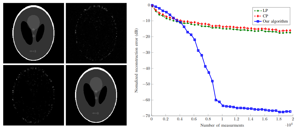
Figure 2: Left block: Reconstruction of Shepp-Logan phantom image of size $256\times 256$ where the picture is split into $64$ blocks of size $32\times 32$, each requires $m=10^{5}$ measurements. Top left image: Ground truth image ($\text{PSNR}=\infty~{}dB$). Top right image: Recovered image via LP ($\text{PSNR}=12.02~{}dB$). Bottom left image: Recovered image via CP ($\text{PSNR}=11.98~{}dB$). Bottom right image: Recovered image via our algorithm ($\text{PSNR}=118.25~{}dB$). Right block: Reconstruction of a dictionary-sparse signal $\bm{x}\in\mathbb{R}^{50}$ in dictionary $\bm{D}\in\mathbb{R}^{50\times 1000}$. The plot shows the reconstruction error averaged over $100$ Monte Carlo simulations for Algorithms LP, CP, and our proposed algorithm.

In the second experiment, we consider the Shepp-Logan phantom image as the ground-truth signal. Since the required number of measurements in one-bit CS is almost high (see e.g. [11] and [12, Section 4.2] ), we split the picture into multiple blocks of size $32\times 32$ and process each block separately. We use redundant wavelet dictionary and $10^{5}$ Gaussian measurements to recover each block. We evaluate the reconstruction quality of final result in terms of the peak signal to noise ratio (PSNR) given by $\text{PSNR}\left(\bm{X},\widehat{\bm{X}}\right)=20\log_{10}\left(\tfrac{\|\bm{X}\|_{\infty}256}{\|\bm{X}-\widehat{\bm{X}}\|_{F}}\right),$ where $\bm{X}$ and $\widehat{\bm{X}}$ are the true and estimated images. As shown by left block of Figure 2, LP and CP algorithms clearly fail with a poor performance but as it is evident in the bottom right image (left block of Figure 2), the output of our algorithm is almost similar to the desired picture.

Appendix A Proof

A-A Proof of Theorem 1

Proof.

By induction law, we show that

$$\|\bm{f}-\bm{f}_{i}\|_{2}\leq\epsilon r2^{1-i}$$ (6)

holds with high probability for any $i\in\{1,\dots,T\}$. Consider the first step i.e. $i=1$ in Algorithm 2. At this step, our initial estimate $\bm{f}_{0}$ is equal to $\bm{0}$. Thus, the output of Algorithm 1 only contains the random part of high dimensional thresholds (step 2 of Algorithm 2). Then, we obtain $\bm{f}_{1}$ by using steps 4-9 of Algorithm 2 (except that we assume $\sigma=r$ in Algorithm 2). As a result, to verify $\|\bm{f}-\bm{f}_{1}\|_{2}\leq\epsilon r$, we use [5, Theorem 8]. Now suppose that the result (6) holds in the $(i-1)$-th step, i.e,

$$\|\bm{f}-\bm{f}_{i-1}\|_{2}\leq\epsilon r2^{2-i}.$$ (7)

Consider $i$-th stage of Algorithm 2 where the high dimension thresholds and the measurements are obtained as

$$\bm{\varphi}^{\left(i\right)}\leftarrow\Phi(\bm{A}^{(i)},q,2^{1-i}r,\bm{f}_{i-1}),$$ (8)

$$\bm{y}^{\left(i\right)}=\text{sign}\left(\bm{A}^{(i)}\bm{f}-\bm{\varphi}^{\left(i\right)}\right).$$ (9)

By substituting (8) in (9), we reach: ‌

$$\bm{y}^{\left(i\right)}=\text{sign}\left(\bm{A}^{(i)}(\bm{f}-\bm{f}_{i-1})-\bm{\tau}^{(i)}\right).$$ (10)

Since $\bm{f}$ is effective $s$-analysis-sparse and the output of Algorithm 2 at the $(i-1)$-th stage, i.e. $\bm{f}_{i-1}$ is effectively $s$-analysis-sparse, the signal $\bm{f}-\bm{f}_{i-1}$ is effectively $4s$-analysis-sparse. Now, we can apply [5, Theorem 8] to this signal. In simple words, we set

$$\bm{f}\leftarrow\bm{f}-\bm{f}_{i-1},r\leftarrow 2^{-i}r,\sigma\leftarrow 2^{-i}r,s\leftarrow 4s$$ (11)

in [5, Theorem 8]. As a result, we shall have that ‌

$$\left\|\bm{f}-\bm{f}_{i-1}-\bm{\Delta}_{i}\right\|_{2}\leq\epsilon 2^{-i}r,$$ (12)

with probability at least $1-\gamma\exp(-c^{\prime}q)$. Now, suppose that (12) occurs. Consider

$$\bm{f}_{\rm tmp}=\bm{f}_{i-1}+\bm{\Delta}_{i}.$$ (13)

After applying step 6 of Algorithm 2, we obtain $\bm{f}_{i}$ that has the property

$$\|\bm{D}^{\rm H}\bm{f}_{i}\|_{1}\leq\sqrt{s}r.$$

Then, we have

$$\|\bm{f}-\bm{f}_{i}\|_{2}\leq\|\bm{f}-\bm{f}_{\rm tmp}\|_{2}+\|\bm{f}_{\rm tmp}-\bm{f}_{i}\|_{2}.$$ (14)

Finally, by using (12), (13), and the fact that $\|\bm{f}_{i}-\bm{f}_{\rm tmp}\|_{2}\leq\|\bm{f}-\bm{f}_{\rm tmp}\|_{2}$ (step 6), the latter equation becomes

$$\|\bm{f}-\bm{f}_{i}\|_{2}\leq\epsilon 2^{1-i}r$$ (15)

Since we consider $T$ stage in Algorithm 2 and 3, we reach the error bound: ‌

$$\left\|\bm{f}-\bm{f}_{T}\right\|_{2}\leq\epsilon r2^{1-T}.$$ (16)

∎

References

- [1] D. L. Donoho, “Compressed sensing,” IEEE Transactions on information theory, vol. 52, no. 4, pp. 1289–1306, 2006.
- [2] E. J. Candès et al., “Compressive sampling,” in Proceedings of the international congress of mathematicians, vol. 3, pp. 1433–1452, Madrid, Spain, 2006.
- [3] P. T. Boufounos and R. G. Baraniuk, “1-bit compressive sensing,” in Information Sciences and Systems, 2008. CISS 2008. 42nd Annual Conference on, pp. 16–21, IEEE, 2008.
- [4] E. J. Candès, Y. C. Eldar, D. Needell, and P. Randall, “Compressed sensing with coherent and redundant dictionaries,” Applied and Computational Harmonic Analysis, vol. 31, pp. 59–73, jul 2011.
- [5] R. Baraniuk, S. Foucart, D. Needell, Y. Plan, and M. Wootters, “One-bit compressive sensing of dictionary-sparse signals,” Information and Inference: A Journal of the IMA, vol. 7, pp. 83–104, aug 2017.
- [6] A. Zymnis, S. Boyd, and E. Candes, “Compressed sensing with quantized measurements,” IEEE Signal Processing Letters, vol. 17, no. 2, pp. 149–152, 2010.
- [7] J. N. Laska and R. G. Baraniuk, “Regime change: Bit-depth versus measurement-rate in compressive sensing,” IEEE Transactions on Signal Processing, vol. 60, no. 7, pp. 3496–3505, 2012.
- [8] L. Jacques, J. N. Laska, P. T. Boufounos, and R. G. Baraniuk, “Robust 1-bit compressive sensing via binary stable embeddings of sparse vectors,” IEEE Transactions on Information Theory, vol. 59, no. 4, pp. 2082–2102, 2013.
- [9] Y. Plan and R. Vershynin, “One-bit compressed sensing by linear programming,” Communications on Pure and Applied Mathematics, vol. 66, no. 8, pp. 1275–1297, 2013.
- [10] U. S. Kamilov, A. Bourquard, A. Amini, and M. Unser, “One-bit measurements with adaptive thresholds,” IEEE Signal Processing Letters, vol. 19, no. 10, pp. 607–610, 2012.
- [11] R. G. Baraniuk, S. Foucart, D. Needell, Y. Plan, and M. Wootters, “Exponential decay of reconstruction error from binary measurements of sparse signals,” IEEE Transactions on Information Theory, vol. 63, no. 6, pp. 3368–3385, 2017.
- [12] D. Needell, R. Saab, and T. Woolf, “Weighted-minimization for sparse recovery under arbitrary prior information,” Information and Inference: A Journal of the IMA, vol. 6, no. 3, pp. 284–309, 2017.