Constraints on anharmonic corrections of Fuzzy Dark Matter

Abstract

The cold dark matter (CDM) scenario has proved successful in cosmology. However, we lack a fundamental understanding of its microscopic nature. Moreover, the apparent disagreement between CDM predictions and subgalactic-structure observations has prompted the debate about its behaviour at small scales. These problems could be alleviated if the dark matter is composed of ultralight fields $m\sim 10^{-22}\ \text{eV}$, usually known as fuzzy dark matter (FDM). Some specific models, with axion-like potentials, have been thoroughly studied and are collectively referred to as ultralight axions (ULAs) or axion-like particles (ALPs). In this work we consider anharmonic corrections to the mass term coming from a repulsive quartic self-interaction. Whenever this anharmonic term dominates, the field behaves as radiation instead of cold matter, modifying the time of matter-radiation equality. Additionally, even for high masses, i.e. masses that reproduce the cold matter behaviour, the presence of anharmonic terms introduce a cut-off in the matter power spectrum through its contribution to the sound speed. We analyze the model and derive constraints using a modified version of class and comparing with CMB and large-scale structure data.

I Introduction

The evidence collected over the last decades suggests that most of the matter in the universe exists in the form of dark matter (DM), whose effects have only been detected through its gravitational interaction. In particular, the assumption that dark matter is composed of non-relativistic particles, the so-called cold dark matter (CDM), has produced a remarkable concordance with the observational data over a wide range of scales and evolution epochs. It is one of the foundations of the succesful standard cosmological model $\Lambda$CDM.

Notwithstanding agreement with observations, several ingredients are lacking in our understanding of DM. In the first place, we have been unable to detect any non-gravitational interaction of DM. Most of the work in the field is currently devoted to direct, indirect detection and production searches. Owing to this effort it has been possible to tighten the parameter space of the most popular models. This lack of additional interactions makes it more difficult to discriminate between different models. There are many candidates that behave like CDM on cosmological scales, with masses ranging from the meV of the QCD axion Graham et al. (2015) to the TeV Goldberg (1983); Ellis et al. (1984) and going up to the 100 $M_{\odot}$ of the primordial black holes Carr et al. (2016). The other ingredient missing is a precise understanding of the DM behaviour on small, i.e. galactic, scales. Even though most DM models mimic CDM on cosmological scales, their predictions usually differ on smaller scales Ostriker and Steinhardt (2003) so they could be discriminated based only on their gravitational effects. In fact, there exist three long-standing debates, questioning the agreement between observations and the CDM theoretical predictions Weinberg et al. (2014); Pontzen and Governato (2014), the so-called ‘too big to fail’ Boylan-Kolchin et al. (2011), ‘missing satellites’ Moore et al. (1999) and especially the ‘core-cusp’ problem de Blok (2010). The ‘core-cusp’ problem refers to the discrepancy between the density profiles of CDM halos obtained in $N$-body simulations, that tend to be cuspy in the center, and the ones inferred from observations, that point to the existence of a central core. Although these problems are sometimes attributed to baryonic effects unaccounted for in the simulations Oñorbe et al. (2015), they remain one of the main challenges of the CDM model.

An interesting alternative that neatly solves the ‘core-cusp’ problem is fuzzy dark matter (FDM) Hu et al. (2000). In this picture, dark matter is composed of ultralight particles with $m\sim 10^{-22}\;\text{eV}$, so that its Compton wavelength ($m^{-1}$) reaches astrophysical scales. Then, the formation of cusps is prevented Schive et al. (2014). The wave nature of the particles on the smallest scales makes them impossible to localize. While solving this problem, FDM behaves as a rapidly oscillating coherent scalar field, thus recovering the CDM behaviour on cosmological scales. In his groundbreaking work Turner (1983), Turner analyzed a homogeneous oscillating scalar field in an expanding universe. He showed that a rapidly oscillating scalar field with a power-law potential $V(\phi)\propto\phi^{n}$ behaves as a perfect fluid with an effective equation of state $w=(n-2)/(n+2)$. More general expressions can be obtained from a version of the virial theorem Johnson and Kamionkowski (2008). The results of Turner show that a massive scalar field, i.e. harmonic potential, oscillating coherently with a frequency much higher than the expansion rate behaves as CDM, at least at the background level. Afterwards, ultralight scalar fields have been thoroughly studied at the perturbation level Johnson and Kamionkowski (2008); Hwang and Noh (2009); Park et al. (2012); Hlozek et al. (2015); Cembranos et al. (2016), proving that the same conclusion holds. Perturbations of coherent oscillating scalar fields admit an effective fluid description with an effective sound speed nearly zero, like CDM. The main cosmological signature of these models is the supression of growth at small scales. Below some Jeans scale $k_{J}^{-1}$ the modes do not grow appreciably, translating into a cut-off in the matter power spectrum Hlozek et al. (2015). Although the work on ultralight fields has been mainly concerned with scalar fields, there are recent results on higher spin fields. It has been shown that abelian vectors at the background Cembranos et al. (2012) and perturbation level Cembranos et al. (2017), non-abelian vectors Cembranos et al. (2013) and arbitrary-spin fields Cembranos et al. (2014) behave in a similar way. Interestingly, the results of Cembranos et al. (2014) show that it is possible to achieve an isotropic model of higher-spin dark matter as long as it is rapidly oscillating.

These ideas have been applied to the axion, a particularly well-motivated DM candidate. The standard QCD axion was initially proposed to solve the strong $CP$ problem Peccei and Quinn (1977); Wilczek (1978); Weinberg (1978) in particle physics. Likewise, the appereance of many light scalar fields seems to be a generic feature of different string-theory scenarios. Some of these fields have a similar origin as the QCD axion, arising from the breaking of an approximate shift symmetry, and are usually known as axion-like particles (ALPs) or ultralight axions (ULAs) Marsh (2016); Hui et al. (2017). ALPs present similar periodic potentials but with a mass much smaller than the QCD axion that could lie in the range of ultralight fields $m\sim 10^{-22}\;\text{eV}$. While behaving like FDM, ALPs have a rich phenomenology based on their assumed interaction with matter. Aside from the standard searches for axions, there is a wealth of dedicated searches and projected experiments on the lookout for ultralight axions. These include studies of the neutral hydrogen distribution in the universe Sarkar et al. (2016); Kobayashi et al. (2017), laboratory constraints based on nuclear interactions Abel et al. (2017), astrophysical bounds Banik et al. (2017); Hirano et al. (2018); Conlon et al. (2018), gravitational wave searches Brito et al. (2017a, b) and analysis of CMB spectral distortions Sarkar et al. (2017); Diacoumis and Wong (2017). A prominent feature of the model is the presence of anharmonic corrections over the mass term in FDM. These corrections arise, to first order, as quartic corrections in the potential with the opposite sign of the mass term, i.e. attractive self-interactions. These effects have been studied, as well as the effect of the full axion potential Ureña-López and Gonzalez-Morales (2016); Cedeño et al. (2017) and their effect on the linear matter power spectrum seems to be negligible. However, self-interactions could modify non-linear structures in a significant way Desjacques et al. (2018)

Another possibility involves introducing a positive quartic correction, i.e. repulsive self-interactions. It is more difficult to find particle-physics models in this case Fan (2016), but the model is nonetheless well motivated as the simplest modification leading to a stable potential. This modification has been previously analyzed in some works Goodman (2000); Li et al. (2014); Suárez and Chavanis (2017); Dev et al. (2017); Li et al. (2017). The additional source of pressure from the repulsive self-interactions helps to solve the ‘core-cusp’ problem with larger masses Fan (2016). Additionaly, unlike the axion case, it could explain the formation of vortices in galaxies Rindler-Daller and Shapiro (2012).

In this work we will consider a fuzzy dark matter model with an additional quartic self-interaction. Using a modified version of the cosmological Boltzmann code class Blas et al. (2011) and parameter-extraction code MontePython Audren et al. (2013) we will constrain the parameters of the model with CMB Ade et al. (2016) and large-scale structure (LSS) Parkinson et al. (2012) data. Section II presents the model and the relevant equations for background and perturbation evolution. In section III, we review the averaging procedure when the field is rapidly oscillating and the effective fluid equations in this case. Section IV discusses a simplified model and estimates analytic bounds on the parameters, highlighting the main physical effects and the origin of the constraints on the model. In section V we present the result of the full numerical analysis and the final constraints on the model, as well as a discussion of its physical origin. Section VI summarizes the conclusions and prospects for future work.

II Exact evolution

Let us assume a scalar field with Lagrangian

$$\mathcal{L}=\frac{1}{2}g^{\mu\nu}\partial_{\mu}\phi\partial_{\nu}\phi-V(\phi),$$ (1)

and potential

$$V(\phi)=\frac{1}{2}m^{2}\phi^{2}+\frac{1}{4}\lambda\phi^{4}\ ,$$ (2)

in a homogeneous and isotropic universe with a flat Robertson-Walker metric in conformal time $\eta$

$$\text{d}s^{2}=a^{2}(\eta)\left(\text{d}\eta^{2}-\text{d}\bm{x}^{2}\right)\ .$$ (3)

The equation of motion for a homogeneous scalar field in this background is

$$\ddot{\phi}+2\mathcal{H}\dot{\phi}+a^{2}V^{\prime}(\phi)=0\ ,$$ (4)

where $\mathcal{H}=\dot{a}/a$ and $\;\;\dot{}\equiv\partial/\partial\eta\;$. We choose initial conditions

$$\phi =\phi_{0}\ ,$$ (5)

$$\dot{\phi} =0\ ,$$ (6)

where $\phi_{0}$ is chosen to match the desired energy density $\Omega_{\phi}$ today. These are the usual initial conditions when the axion-like particles are produced through a misalignment mechanism Diez-Tejedor and Marsh (2017) and the field starts its evolution frozen. It is important to note that the choice of initial conditions has a deep impact in the subsequent evolution. In Li et al. (2014), the authors considered a case similar to ours, but with an initial velocity $\dot{\phi}\neq 0$. In this case, there is an initial phase of stiff-matter domination, absent in our case, constrained to be short enough not to spoil BBN.

We now introduce scalar perturbations over a flat Robertson-Walker metric. Following the notation of Mukhanov et al. (1992), the general form of the perturbations is

$$\text{d}s^{2}=a^{2}(\eta)\Bigg{[}(1+2\Phi)\text{d}\eta^{2}-2\partial_{i}B\text{d}x^{i}\text{d}\eta-\Big{(}(1-2\Psi)\delta_{ij}+2\partial_{i}\partial_{j}E\Big{)}\text{d}x^{i}\text{d}x^{j}\Bigg{]}\ .$$ (7)

The equation of motion for the scalar field perturbation is

$$\ddot{\delta\phi}+2\mathcal{H}\dot{\delta\phi}+(k^{2}+a^{2}V^{\prime\prime})\delta\phi=\Big{(}k^{2}(B-\dot{E})+\dot{\Phi}+3\dot{\Psi}\Big{)}\dot{\phi}-2a^{2}\Phi V^{\prime}\ ,$$ (8)

where the gauge has not yet been fixed. We can introduce a different parameterization, reminiscent of a perfect fluid. The components of the perturbed energy-momentum tensor are Mukhanov et al. (1992)

$$\delta T^{0}_{\phantom{a}0} \equiv\delta\rho_{\phi}=a^{-2}(\dot{\phi}\dot{\delta\phi}-\dot{\phi}^{2}\Phi)+V^{\prime}\delta\phi\ ,$$ (9)

$$\delta T^{i}_{\phantom{a}j} \equiv-\delta P_{\phi}\,\delta^{i}_{j}=-\Big{(}a^{-2}(\dot{\phi}\dot{\delta\phi}-\dot{\phi}^{2}\Phi)-V^{\prime}\delta\phi\Big{)}\,\delta^{i}_{j}\ ,$$ (10)

$$\delta T^{0}_{\phantom{a}i} \equiv(\rho_{\phi}+P_{\phi})(v^{i}_{\phi}-\partial_{i}B)=a^{-2}\dot{\phi}\,\partial_{i}\delta\phi\ .$$ (11)

We can rewrite (8) in terms of the fluid variables, introducing $\delta=\delta\rho/\rho$ and $u=(1+w)(v-B)$. In the synchronous gauge, the metric variables read

$$\Psi =-\frac{1}{6}\big{(}h-\nabla^{2}\mu\big{)}\ ,$$

$$E =\frac{1}{2}\mu\ ,$$

$$\Phi =B=0\ ,$$

and the equations of motion are

$$\dot{\delta} =-3\mathcal{H}(1-w)\delta-ku-9\mathcal{H}^{2}(1-c^{2}_{\text{ad}})\frac{u}{k}-\frac{1}{2}(1+w)\dot{h}\ ,$$ (12)

$$\dot{u} =2\mathcal{H}u+k\delta+3(w-c^{2}_{\text{ad}})\mathcal{H}u\ ,$$ (13)

where $w=P/\rho$ is the equation of state and the adiabatic sound speed $c^{2}_{\text{ad}}$ is

$$c^{2}_{\text{ad}}=\frac{\dot{P}}{\dot{\rho}}=1+\frac{2}{3}\frac{a^{2}V^{\prime}}{\mathcal{H}\dot{\phi}}\ .$$ (14)

Following the analysis of Hlozek et al. (2015) we provide the system with initial conditions

$$\delta =0\ ,$$ (15)

$$u =0\ ,$$ (16)

valid up to corrections of order $(k\eta)^{4}$. The scalar field starts its evolution frozen in a value $\phi_{0}$ with an equation of state $w\simeq-1$. As the universe expands the field starts rolling down the potential, when it reaches the minimum it undergoes rapid oscillations. These oscillations occur when the effective frequency $\omega_{\text{eff}}\sim\sqrt{V^{\prime\prime}(\phi)}$ is bigger than the friction term $\mathcal{H}$, so once the scalar field starts oscillating its frequency becomes much larger than the expansion rate, the inverse of the evolution time scale of the background.

On the numerical side, this means that it becomes prohibitely expensive to compute the exact evolution of the field, following every oscillation. However, the huge difference between time scales allows us to average the equations of motion and turn to an effective description.

III Averaged evolution

The study of the cosmological evolution of a fast oscillating scalar was first performed in Turner (1983). Basically, if the oscillation frequency of the scalar field is much higher than the expansion rate of the universe, the cosmological evolution becomes independent of the periodic phase of the field at leading order. Consequently, the Einstein equations can be approximately solved averaging in time the energy-momentum tensor

$$G^{\mu}_{\phantom{a}\nu}=8\pi G\left\langle T^{\mu}_{\phantom{a}\nu}\right\rangle\ ,$$ (17)

where

$$\left\langle T^{\mu}_{\phantom{a}\nu}\right\rangle(t)=\frac{1}{T}\int^{t+T/2}_{t-T/2}T^{\mu}_{\phantom{a}\nu}(t^{\prime})\text{d}t^{\prime}\ .$$ (18)

If the field is periodic, we can consider an integer number of periods as the integration interval. However, similar results can be reached for fast-evolving bounded solutions averaging over time spans much bigger than the inverse of its frequency but much smaller than the inverse of the expansion rate, $\omega^{-1}\ll T\ll\mathcal{H}^{-1}$. The averaging error in both cases results $\mathcal{O}(\mathcal{H}T)$.

To leading order we can drop the averages of total time derivatives, so it can be proved Cembranos et al. (2016) that

$$\left\langle\dot{\phi}^{2}/a^{2}\right\rangle=-\left\langle\phi\ddot{\phi}/a^{2}\right\rangle=\left\langle V^{\prime}(\phi)\phi\right\rangle+\mathcal{O}\Big{(}\frac{\mathcal{H}}{\omega_{\text{eff}}}\Big{)}\ ,$$ (19)

and with this result the effective equation of state can be written as

$$w=\frac{\left\langle p\right\rangle}{\left\langle\rho\right\rangle}=\frac{\left\langle V^{\prime}\phi-2V\right\rangle}{\left\langle V^{\prime}\phi+2V\right\rangle}=\frac{n-2}{n+2}+\mathcal{O}\Big{(}\frac{\mathcal{H}}{\omega_{\text{eff}}}\Big{)}\ ,$$ (20)

for power-law potentials $V(\phi)\propto\phi^{n}$. As it can be seen, a massive scalar field, $V=m^{2}\phi^{2}/2$, would behave as CDM. For this particular case we can solve the equation of motion through a WKB expansion. Thanks to this adiabatic expansion in the parameter $\mathcal{O}(\mathcal{H}/ma)$ we can perform the averages explicitly, isolating the fast evolving factor and integrating by parts, as explained in Cembranos et al. (2016). For our model, we must compute the first correction in $\lambda$. If the mass term is dominant, via a WKB expansion we can write

$$\left\langle\phi^{4}\right\rangle \simeq\frac{3}{2}\left\langle\phi^{2}\right\rangle\left\langle\phi^{2}\right\rangle\ ,$$ (21)

$$\left\langle\rho\right\rangle \simeq m^{2}\left\langle\phi^{2}\right\rangle\ ,$$ (22)

so the first anharmonic correction to the equation of state is

$$w\simeq\frac{3\lambda}{8m^{4}}\left\langle\rho\right\rangle\ .$$ (23)

In this effective description the background evolution of the field is described through its density and its effective equation of state, using the conservation equation

$$\dot{\rho}=-3\mathcal{H}(1+w)\rho\ .$$ (24)

where for the equation of state $w$ we will use the formula

$$w=\frac{\displaystyle\frac{3\lambda}{8m^{4}}\rho}{\displaystyle 1+\frac{9\lambda}{8m^{4}}\rho}\ ,$$ (25)

that smoothly interpolates between the radiation-like $w\simeq 1/3$ and matter-like $w\simeq 0$ behaviour. Now we can apply the same trick to the evolution of the perturbations. The equations of motion for the fluid variables are

$$\dot{\delta} =3\mathcal{H}(w-c_{s}^{2})\delta-ku-\frac{1}{2}(1+w)\dot{h}\ ,$$ (26)

$$\dot{u} =-\mathcal{H}(1-3w)u+kc_{s}^{2}\delta\ ,$$ (27)

where $\delta\equiv\left\langle\delta\rho\right\rangle/\left\langle\rho\right\rangle$, $u\equiv(1+w)\left\langle v\right\rangle$ stand for averaged quantities and $w$, $c_{s}^{2}$ are the effective equation of state and sound speed. To complete the system there only remains to compute the effective sound speed

$$c_{s}^{2}=\frac{\left\langle\delta P\right\rangle}{\left\langle\delta\rho\right\rangle}\ .$$ (28)

In contrast with the adiabatic sound speed, the sound speed is gauge-dependent. But, as we will show now, the gauge ambiguities remain of order $\mathcal{O}(\mathcal{H}/\omega_{\text{eff}})$ so our effective sound speed turns out to be gauge-independent. In fact, identical expressions have previously been obtained working in the comoving gauge Li et al. (2014) and in the Newtonian gauge (Cembranos et al., 2016). To leading order we have

$$\left\langle\partial_{\eta}(\dot{\phi}\delta\phi+\phi\delta\dot{\phi})\right\rangle =0+\mathcal{O}\Big{(}\frac{\mathcal{H}}{\omega_{\text{eff}}}\Big{)}\ .$$ (29)

Then, using (8) and (29) we can obtain the result

$$\left\langle\dot{\phi}\dot{\delta\phi}\right\rangle=\frac{1}{2}\left\langle a^{2}V^{\prime}\delta\phi+(k^{2}+a^{2}V^{\prime\prime})\phi\delta\phi\right\rangle+\Phi\left\langle a^{2}V^{\prime}\phi\right\rangle+\mathcal{O}\Big{(}\frac{\mathcal{H}}{\omega_{\text{eff}}}\Big{)}\ ,$$ (30)

and finally compute the effective sound speed for a generic gauge

$$c_{s}^{2} =\frac{\left\langle\delta P\right\rangle}{\left\langle\delta\rho\right\rangle}=\frac{\frac{1}{2}\left\langle V^{\prime}\delta\phi+((k/a)^{2}+V^{\prime\prime})\phi\delta\phi-2V^{\prime}\delta\phi\right\rangle-\Phi\left\langle\dot{\phi}^{2}/a^{2}-V^{\prime}\phi\right\rangle}{\frac{1}{2}\left\langle V^{\prime}\delta\phi+((k/a)^{2}+V^{\prime\prime})\phi\delta\phi+2V^{\prime}\delta\phi\right\rangle-\Phi\left\langle\dot{\phi}^{2}/a^{2}-V^{\prime}\phi\right\rangle}+\mathcal{O}\Big{(}\frac{\mathcal{H}}{\omega_{\text{eff}}}\Big{)}$$ (31)

$$=\frac{\left\langle((k/a)^{2}+V^{\prime\prime})\phi\delta\phi-V^{\prime}\delta\phi\right\rangle}{\left\langle((k/a)^{2}+V^{\prime\prime})\phi\delta\phi+3V^{\prime}\delta\phi\right\rangle}+\mathcal{O}\Big{(}\frac{\mathcal{H}}{\omega_{\text{eff}}}\Big{)}\ .$$ (32)

As we anticipated, the gauge ambiguities in the metric perturbations remain of order $\mathcal{O}(\mathcal{H}/\omega_{\text{eff}})$, so the final expression holds in any gauge. Moreover, it can be rewritten in a manifestly gauge-invariant form substituting $\delta\phi$ by its gauge-invariant perturbation Mukhanov et al. (1992)

$$\delta\phi^{\text{(gi)}}=\delta\phi+\dot{\phi}(B-\dot{E})\ ,$$ (33)

and using the relations

$$\left\langle V^{\prime}\dot{\phi}\right\rangle =\left\langle\partial_{\eta}(V)\right\rangle=0+\mathcal{O}\Big{(}\frac{\mathcal{H}}{\omega_{\text{eff}}}\Big{)}\ ,$$ (34)

$$\left\langle V^{\prime\prime}\phi\dot{\phi}\right\rangle =\left\langle\phi\,\partial_{\eta}(V^{\prime})\right\rangle=-\left\langle V^{\prime}\dot{\phi}\right\rangle+\mathcal{O}\Big{(}\frac{\mathcal{H}}{\omega_{\text{eff}}}\Big{)}=0+\mathcal{O}\Big{(}\frac{\mathcal{H}}{\omega_{\text{eff}}}\Big{)}\ ,$$ (35)

we obtain

$$c_{s}^{2}=\frac{\left\langle((k/a)^{2}+V^{\prime\prime})\phi\delta\phi^{\text{(gi)}}-V^{\prime}\delta\phi^{\text{(gi)}}\right\rangle}{\left\langle((k/a)^{2}+V^{\prime\prime})\phi\delta\phi^{\text{(gi)}}+3V^{\prime}\delta\phi^{\text{(gi)}}\right\rangle}+\mathcal{O}\Big{(}\frac{\mathcal{H}}{\omega_{\text{eff}}}\Big{)}\ .$$ (36)

This expression agrees with the result obtained in Cembranos et al. (2016) working in the Newtonian gauge, so the same conclusions apply. In particular, a generic feature of this kind of models is a suppression of growth $c^{2}_{s}\simeq 1$ for small scales $k\gg\omega_{\text{eff}}$. In the case of a power-law potential $V(\phi)=\frac{C}{n}\phi^{n}$, for large scales $k\ll\omega_{\text{eff}}$ we have

$$c^{2}_{s}=\frac{n-2}{n+2}+\mathcal{O}\Big{(}\frac{\mathcal{H}}{\omega_{\text{eff}}}\Big{)}\ .$$ (37)

For a harmonic potential $n=2$, the zero-order term drops out and we must calculate the first-order corrections in $k$. Our potential of interest is a polynomial $V(\phi)=\frac{1}{2}m^{2}\phi^{2}+\frac{\lambda}{4}\phi^{4}$, a mass term plus an anharmonic correction, in this case we have Cembranos et al. (2016)

$$c^{2}_{s}=\frac{k^{2}}{4m^{2}a^{2}}+\frac{3}{4}\frac{\lambda}{m^{4}}\rho\ ,$$ (38)

where $\rho$ is the energy density of the scalar field and the anharmonic correction is assumed to be small. In our numerical solution we will use an effective sound speed

$$c_{s}^{2}=\frac{\displaystyle\Big{(}\frac{k}{2ma}\Big{)}^{2}+\frac{3}{4}\frac{\lambda}{m^{4}}\rho}{1+\displaystyle\Big{(}\frac{k}{2ma}\Big{)}^{2}+\frac{9}{4}\frac{\lambda}{m^{4}}\rho}\ ,$$ (39)

suggested by the form of (32) and that smoothly interpolates between all the regimes of interest.

IV Heuristic constraints on the non-harmonic contribution

In this section we will discuss the simplest limits that constrain the model. With this objective let us assume a simple cosmology composed of radiation, cosmological constant and our scalar field

$$\mathcal{H}^{2}=a^{2}H_{0}^{2}\left(\Omega_{\phi}(a)+\frac{\Omega_{\text{rad}}}{a^{4}}+\Omega_{\Lambda}\right)\ ,$$ (40)

where $\Omega_{i}=8\pi G\rho_{i}/(3H_{0}^{2})$ are the abundances with $i\in\{\phi,\text{rad},\Lambda\}$ which correspond to scalar field, radiation and cosmological constant respectively.

• Limits on $\lambda$ from background evolution. The position of the peaks in the CMB temperature spectrum, especially the first one, is very sensitive to the amount of matter and the redshift of equality $z_{\text{eq}}$. We can assume that to have a viable model of dark matter this quantities remain essentially the same as in $\Lambda$CDM. In this case, to have a dark matter behaviour that resemble CDM the anharmonic corrections at this time should be small

  $$1\gg w\simeq\frac{3}{8}\frac{\lambda}{m^{4}}\rho_{\phi}(a_{\text{eq}})\ .$$ (41)

  This imposes an upper limit on $\lambda$, namely

  $$\lambda<\frac{8}{3}\frac{m^{4}}{\rho_{\phi}(a_{\text{eq}})}\ ,$$ (42)

  excluding the orange region in Figure 1.
  

• Limits on $m$ from perturbation evolution. If $\lambda$ is small enough, the background evolution of the effective fluid is identical to $\Lambda$CDM. In this case we can obtain limits from the behaviour of the perturbations. From (26) and (27) it can be seen that if we neglect the expansion rate, $c_{s}^{2}k^{2}\gg\mathcal{H}^{2}$, density perturbations evolve according to

  $$\ddot{\delta}\simeq-c_{s}^{2}k^{2}\delta\ .$$ (43)

  producing an oscillatory behaviour instead of the standard growth. To avoid a clear disagreement with observations, the effect of a non-negligible sound speed must be small

  $$c_{s}^{2}k^{2}<\mathcal{H}^{2}\ .$$ (44)

  Translating into a lower bound in the allowed masses

  $$m>\frac{k^{2}}{2a\mathcal{H}}\ ,$$ (45)

  as before, we assume that $z_{\text{eq}}$ corresponds to the standard value. To obtain a conservative limit we choose $k=0.2\ \text{Mpc}^{-1}$, the highest mode observed in LSS at the linear level, so that

  $$m\mbox{\raisebox{-3.87495pt}{~{}$\stackrel{{\scriptstyle\mbox{$>$}}}{{\sim}}$~{}}}10^{-26}\ \text{eV}\ ,$$ (46)

  excluding the blue region in Figure 1.
  

• Observable effects of anharmonic corrections. Finally, there is a region in the parameter space that we cannot yet exclude and where the effects of anharmonic corrections to the sound speed may be important

  $$c_{s}^{2}\simeq\frac{k^{2}}{4m^{2}a^{2}}+\frac{3}{4}\frac{\lambda}{m^{4}}\rho_{\phi}\ .$$ (47)

  Imposing that the second term dominates over the harmonic contribution yields an upper bound on $\lambda$

  $$\lambda>\frac{k^{2}m^{2}}{3\rho_{\phi}a^{2}}\ ,$$ (48)

  corresponding to a region that we cannot exclude right away, but where effects of the anharmonic corrections to the sound speed are to be expected.
  

An additional result that can be obtained from (44) is the Jeans wavenumber

$$c_{s}^{2}k_{J}^{2}=\mathcal{H}\ .$$ (49)

Sub-Hubble modes below this Jeans wavenumber, $k<k_{J}$, grow while modes with $k>k_{J}$ are suppressed. In the massive case with $\lambda=0$ we obtain

$$k_{J}^{2}=2a\mathcal{H}m\ .$$ (50)

Now, since we have seen that the quartic correction affects the sound speed, it will also affect the Jeans scale. It is natural to ask what combination of parameters ($m$, $\lambda$) can have a similar impact on structure formation as the case ($\tilde{m}$, $\tilde{\lambda}=0$). To this end, we look for the combination that gives the same Jeans scale at the matter-radiation equality. Since its scaling in time is not significantly modified, this simple estimate should capture the essential features of structure formation in both models. Equating both sound speeds and inserting the result (50) we have an estimate for $\lambda$

$$\lambda=4.96\times 10^{-100}\,\Big{(}\frac{\tilde{m}}{10^{-24}\ \text{eV}}\Big{)}^{3}\Big{(}\frac{1-r^{2}}{r^{4}}\Big{)}\ ,\qquad r\equiv\frac{\tilde{m}}{m}\ .$$ (51)

This simple result suggests for instance that, at the linear level, structure formation should be similar in the models ($\tilde{m}=10^{-26}\ \text{eV}$, $\tilde{\lambda}=0$) and ($m=10^{-24}\ \text{eV}$, $\lambda\simeq 4.96\times 10^{-98}$), a result that we will check with the full numerical solution. This estimate is represented in Figure 1 for two different masses $\tilde{m}$.

After discussing some approximate bounds on our model and its physical origin, we will devote the next section to the full numerical solution.

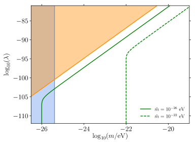
Figure 1: Different heuristic bounds. Orange region corresponds to the parameter-space excluded for the effects of $\lambda$ on the background evolution. In the blue region, the effect of a non-negligible sound speed results in a strong disagreement with observations, hence it is excluded. The green curves represent (51) for two different masses. According to the argument in the main text, points along each curve should give similar structure-formation results.

V Numerical evolution and constraints

We modify the publicly available Boltzmann code class (Blas et al., 2011) and include this ultralight scalar field as a new species, that will assume the role of dark matter. Now, we summarize the key changes in the code and the evolution scheme chosen for the scalar field.

• At the background level, we start solving the equation (4) with initial conditions $\dot{\phi}=0$ and $\phi=\phi_{0}$. The initial value $\phi_{0}$ is chosen internally with a built-in shooting algorithm such as to match the energy density $\Omega_{\phi}$(today) required. As a technical aside, it is critical to start with a sensible initial guess for $\phi_{0}$, so that the shooting algorithm converges quickly. In (Hlozek et al., 2015) the authors provide analytical formulae for the initial guess in the harmonic case, that works as well if the anharmonic corrections are small. If the quadratic and quartic terms are comparable it is more difficult to find analytical expressions that fit our purposes. In our case, we precompute an interpolation table for different values of $m$, $\lambda$ and $\phi_{0}$ yielding some value $\Omega_{\phi}(m,\lambda,\phi_{0})$. We only compute a coarse table, so that we still use the shooting algorithm to adjust $\phi_{0}$ and achieve the desired precision in $\Omega_{\phi}$.

  With the initial conditions provided, the field starts its evolution frozen, slowly rolling down the potential until its natural frequency term in (4) dominates and it undergoes rapid oscillations. In this case it is computationally expensive to follow every oscillation so we turn to the averaged equations when $\sqrt{V^{\prime\prime}(\phi)}>3H$.

  In the averaged regime, we solve (24), matching continuously with the solution in the exact regime, and compute the pressure using the effective equation of state (25).

• At the perturbation level, we first solve (12) and (13) with adiabatic initial conditions $\delta=u=0$. For each mode $k$ we start the integration early enough to ensure that we start well within the exact regime, $\sqrt{V^{\prime\prime}(\phi)}\ll 3H$. In the averaged regime, $\sqrt{V^{\prime\prime}(\phi)}>3H$, we solve the equations (26) and (27) with the sound speed given by (39).

Some results for temperature and matter power spectra are shown in Figures 2 and 3. They show the impact of different choices of $m$ and $\lambda$, while the other cosmological parameters are fixed to their Planck (Ade et al., 2016) best-fit values. As anticipated, the main cosmological signature is the appearance of a cut-off in the matter power spectrum. This cut-off has already been discussed in the harmonic case Hlozek et al. (2015). In our case, we see that the anharmonic terms produce a similar effect.

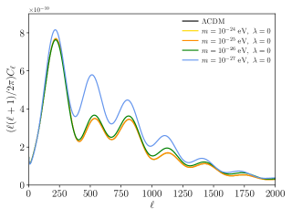
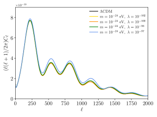
Figure 2: Temperature power spectrum. On the left, results for a massive scalar field without self-interaction. On the right, results for different self-interaction strengths for a mass that is indistinguishable from CDM with $\lambda=0$.

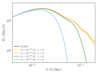
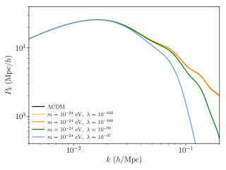
Figure 3: Matter power spectrum. On the left, results for a massive scalar field without self-interaction. On the right, results for different self-interaction strengths for a mass that is indistinguishable from CDM with $\lambda=0$.

V.1 Physical effects

The main physical effect responsible for the appearance of a cut-off in the matter power spectrum has already been discussed. In the averaged regime, the scalar field that supplies the dark matter component behaves like a fluid with a non-negligible sound speed. On small scales, above a certain Jeans scale $k_{J}$, the density perturbations oscillate and the growth is suppressed. This effect is illustrated in the Figure 4 for modes above and below $k_{J}$.

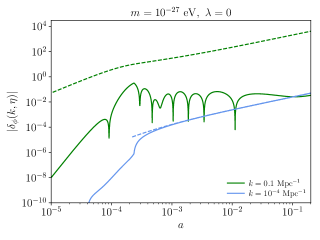
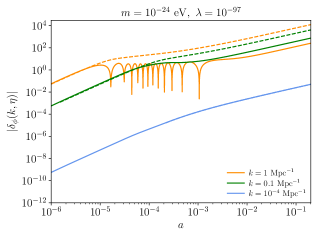
Figure 4: Evolution in time of the dark matter transfer functions compared to the standard $\Lambda$CDM evolution, represented by dotted lines.

In the case of the CMB temperature power spectrum, it is far more difficult to disentangle the physical effect responsible for each feature. We split the effects in two categories, those coming from the modified background evolution and those coming from the perturbations. Furthermore, we will refer to two extreme cases $(m=10^{-27},\ \lambda=0)$ and $(m=10^{-24},\ \lambda=10^{-97})$ as $m$-case and $\lambda$-case respectively. To gain some insight into the CMB spectrum structure, we will rely on simplified, analytical estimates Hu and Sugiyama (1996); Weinberg (2008); Lesgourgues (2013) and work in the Newtonian gauge.

Background evolution

The modified equation of state (25) changes the background evolution, modifying in particular the redshift of matter-radiation equality $z_{\text{eq}}$ and in general the expansion history $a(\tau)$. In the $m$-case, the field transitions directly from the frozen value $w\simeq-1$ to a matter-like phase, while in the $\lambda$-case there is an intermediate radiation-like phase. There are two key effects

• First peak position. The position $\ell_{\text{peak}}$ of the first peak can be estimated as

  $$\theta_{\text{peak}}=\frac{\pi}{\ell_{\text{peak}}}\simeq\frac{d_{s}\rvert_{\text{dec}}}{d_{a}\rvert_{\text{dec}}}\ ,$$ (52)

  where the angular diameter $d_{a}$ distance is defined as

  $$d_{a}\rvert_{\text{dec}}=a_{\text{dec}}\int^{\eta_{0}}_{\eta_{\text{dec}}}\text{d}\eta\ ,$$ (53)

  $d_{s}\rvert_{\text{dec}}$ is the sound horizon of the photon-baryon plasma evaluated at decoupling

  $$d_{s}\rvert_{\text{dec}}=a_{\text{dec}}\int^{\eta_{\text{dec}}}_{0}c_{s\,\gamma}\text{d}\eta\ ,$$ (54)

  and the sound speed for the baryon-photon plasma is

  $$c_{s\,\gamma}^{2}=\frac{1}{3(1+R)}\ ,\qquad R\equiv\frac{3\rho_{b}}{4\rho_{\gamma}}\ .$$ (55)

  The angular diameter distance is almost unaffected but the sound horizon is slightly modified. Compared to $\Lambda$CDM we obtain relative deviations on $\ell_{\text{peak}}$ of about $+2\%$, shift to the left, in the $m$-case and $-0.7\%$, shift to the right, in the $\lambda$-case. Both are compatible with the tiny deviations observed in Figure 2.

• Damping envelope. Another physical scale that is modified is the diffusion length

  $$\lambda_{D}\rvert_{\text{dec}}=a_{\text{dec}}\Big{(}\int^{\eta_{\text{dec}}}_{0}\Gamma^{-1}\text{d}\eta\ \Big{)}^{1/2}\ ,$$ (56)

  where

  $$\Gamma=an_{e}\sigma_{T}x_{e}=-\dot{\kappa}\,x_{e}\ ,$$ (57)

  is the Thomson scattering rate. The diffusion length governs the damping envelope, $\text{e}^{-(\ell/\ell_{D})^{2}}$, through the relation

  $$\theta_{D}=\frac{\pi}{\ell_{D}}\simeq\frac{\lambda_{D}\rvert_{\text{dec}}}{d_{a}\rvert_{\text{dec}}}\ .$$ (58)

  For a reference multipole $\ell=820$, corresponding to the third acoustic peak, in the $\lambda$-case we obtain a modified damping envelope that produces an enhancement of $6\%$ compared to $\Lambda$CDM, that can explain the overall increase of power in Figure 2. For the $m$-case, we obtain the puzzling result of a suppression of $0.7\%$, in clear disagreement with the observed effect. However, we will shortly see how a novel effect in the perturbation evolution can account for this overall amplification.

Perturbation evolution

In the tightly coupled regime, the photon temperature fluctuation evolves according to

$$\ddot{\Theta}_{0}+\frac{\dot{R}}{1+R}\dot{\Theta}_{0}+k^{2}c_{s\,\gamma}^{2}\Theta_{0}=-\frac{k^{2}}{3}\psi+\frac{\dot{R}}{1+R}\dot{\phi}+\ddot{\phi}\ ,$$ (59)

In the standard scenario, ignoring slow changes in $R$, $\phi$ and $\psi$ from the expansion, we have

$$\ddot{\Theta}_{0}+k^{2}c_{s\,\gamma}^{2}\Theta_{0}\simeq-\frac{k^{2}}{3}\psi\ .$$ (60)

This produces an oscillatory pattern with frequency $\omega=kc_{s\,\gamma}$ and zero-point displaced by an amount $-(1+R)\psi$. The main part of the temperature Sachs-Wolfe effect comes from the contribution $|\Theta_{0}+\psi|^{2}\rvert_{\text{dec}}$, so the displacement of the zero-point of the oscillations gives the characteristic asymmetry between odd and even peaks in the CMB temperature spectrum. Our modification of dark matter produces two interrelated effects, oscillation and suppression of growth at small scales.

• Effects of suppression of growth at small scales. The suppression of dark matter density perturbations at small scales also suppresses the gravitational wells $\psi$, shifting the zero-point of the oscillation back to zero. This effect, alone, reduces the asymmetry among the peaks, decreasing the odd and increasing the even peaks. This explains the characteristic enhancement of the second peak with respect to the third one in Figure 2.

• Effects of oscillatory behaviour. There only remains to explain one effect, the striking gain in peak amplitude in the $m$-case. According to the modification in the damping envelope, the peaks should be slightly suppressed and their enhancement is actually related to a resonance effect. In the standard scenario, the term $\psi$ behaves like a constant external force, shifting the equilibrium position of the photon oscillations. In our case, it is not constant anymore, but oscillates with a frequency $kc_{s}$ given by the sound speed of the dark matter perturbations (39). These two frequencies, $kc_{s}$ and $kc_{s\,\gamma}$, are comparable for a range of $k$ values, as shown in Figure 5, producing a resonant effect that increases the height of the peaks, as shown in Figure 6.

  

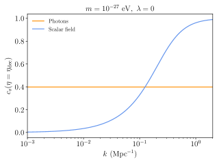
  Figure 5: Sound speed at decoupling for photons and dark matter. Around $k\simeq 0.1\ \text{Mpc}^{-1}$ the sound speed for both fluids, hence the oscillation frequency too, are close and we have a resonant driving.

  

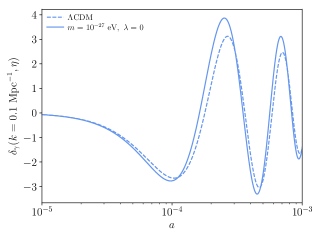
  Figure 6: Evolution in time of the mode $k=0.1\ \text{Mpc}^{-1}$, corresponding approximately to the fifth acoustic peak, until decoupling.

  Moreover, since according to (39) the scale of the crossover in Figure 5 evolves $\propto a$, as we go from decoupling back in time it moves to smaller $k$. That is to say, although the crossover at decoupling is located around $k\simeq 0.1\ \text{Mpc}^{-1}$, smaller $k$ have also fulfilled the resonance condition at previous times, so they have also got amplified.

V.2 Observational constraints

To compare this model with CMB and LSS observations and refine the heuristic constraints obtained in section IV, we use the public parameter-extraction code MontePython (Audren et al., 2013). We will compare our results with two different data sets: CMB measurements by Planck and large-scale structure information by WiggleZ Parkinson et al. (2012). We perform two analysis, Planck only and Planck+WiggleZ. In each case we vary the six $\Lambda$CDM base model parameters, in addition to the foreground parameters, plus $m$ and $\lambda$, the mass and anharmonic parameter. We choose logarithmic priors in our model parameters, as shown in Table 1.

Table 1: Prior ranges on the base $\Lambda$CDM parameters and the model parameters $m$ and $\lambda$. A symbol $-$ means that there is no prior. Additionally, the fixed parameters include the neutrino properties. In our case, two massless neutrinos plus a massive one with $m=0.06\;\text{eV}$, such that $N_{\text{eff}}=3.046$ and $m_{\nu}/\Omega_{\nu}=93.14\;\text{eV}$.

Parameter	minimum	maximum
$\Omega_{b}h^{2}$	$-$	$-$
$\Omega_{\phi}h^{2}$	$-$	$-$
$h$	$-$	$-$
$\log(10^{10}A_{s})$	$-$	$-$
$n_{s}$	$-$	$-$
$\tau_{\text{reio}}^{2}$	$0.04$	$-$
$\log_{10}(m/\text{eV})$	$-26$	$-23.3$
$\log_{10}(\lambda)$	$-111$	$-98$

It is important to note that to perform an accurate comparison with LSS data we must restrict our analysis to linear scales $k\mbox{\raisebox{-3.87495pt}{~{}$\stackrel{{\scriptstyle\mbox{$<$}}}{{\sim}}$~{}}}0.2\ h/\text{Mpc}$. The non-linear module in class includes HaloFit Bird et al. (2012), but since it has not been calibrated for our model we restrict our analysis to linear scales without non-linear corrections. It is to be expected that, in the future, as more $N$-body simulations with ultralight fields become available, non-linear information will allow us to tighten the constraints.

We do not observe any significant degeneracy between $m$, $\lambda$ and the rest of cosmological parameters. Best-fit results are shown in Table 2, while the marginalized countour for our model parameters is represented in Figure 7.

Table 2: Best fit results with 95$\%$ confidence level.

Base parameters	Planck	Planck+WiggleZ
$\Omega_{b}h^{2}$	$0.02223\pm 0.00047$	$0.02212^{+0.00042}_{-0.00041}$
$\Omega_{\phi}h^{2}$	$0.1189^{+0.0044}_{-0.0041}$	$0.1204^{+0.0032}_{-0.0034}$
$h$	$0.677\pm 0.019$	$0.670^{+0.016}_{-0.014}$
$\log(10^{10}A_{s})$	$3.070^{+0.056}_{-0.053}$	$3.057^{+0.046}_{-0.041}$
$n_{s}$	$0.965^{+0.016}_{-0.021}$	$0.963^{+0.011}_{-0.010}$
$\tau_{\text{reio}}^{2}$	$0.070^{+0.028}_{-0.029}$	$0.061^{+0.024}_{-0.021}$
$\log_{10}(m/\text{eV})$	$>-24.5$	$>-24.4$
$\log_{10}(\lambda)$	$-$	$<-99.0$
Derived parameters
$z_{\text{reio}}$	$9.2^{+2.6}_{-2.7}$	$8.4^{+2.2}_{-2.1}$
$\Omega_{\Lambda}$	$0.690^{+0.024}_{-0.027}$	$0.681\pm 0.021$
$Y_{\text{He}}$	$0.24778\pm 0.00020$	$0.24773\pm 0.00018$
$100\theta_{s}$	$1.04193^{+0.00098}_{-0.00099}$	$1.04182^{+0.00084}_{-0.00083}$

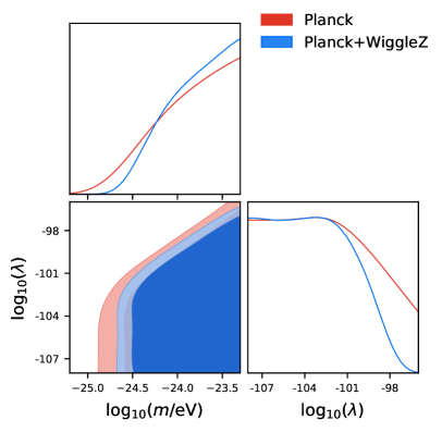
Figure 7: Contour plots with $95\%$ and $99\%$ confidence levels and 1d marginalized distributions.

VI Conclusions

The presence of self-interactions in the ultralight field potential can lead to the appearance of new background-evolution phases, like the radiation-like due to our quartic potential. This modified background evolution, and especially its critical effect on the sound speed of dark matter perturbations, can lead to significant differences from observations. The observational signatures of the anharmonic contribution are similar to the mass term, the most prominent being the appearance of a cut-off in the matter power spectrum. This produces constraints for masses that would be otherwise indistinguishable from CDM, i.e. $m\mbox{\raisebox{-3.87495pt}{~{}$\stackrel{{\scriptstyle\mbox{$>$}}}{{\sim}}$~{}}}10^{-24}\;\text{eV}$. Our constraints on $\lambda$ complement other bounds present in the literature, e.g. Dev et al. (2017). This bounds on $\lambda$ follow a scaling law with $m^{4}$ according to (42). We can extrapolate the results to higher masses using the $2\sigma$ region of Figure 7, obtaining an approximate constraint on $\lambda$

$$\log_{10}(\lambda)<-91.86+4\log_{10}\Big{(}\frac{m}{10^{-22}\ \text{eV}}\Big{)}\ ,$$ (61)

for masses $m>10^{-24}\ \text{eV}$.

So far, we have only analyzed linear observables, but in fact larger effects on non-linear scales are expected. The available parameter space could be further constrained in the future using cosmological information with non-linear observables, as more simulations with ultralight fields become available. Even without non-linear information, using the formula (51) one could put forward the proposal that similar results on structure formation could be obtained for higher masses with a positive $\lambda$. For instance, results for $\tilde{m}=10^{-22}\ \text{eV}$ might be reproduced with masses $m\simeq 10^{-5}\ \text{eV}$ adding a self-interaction of the order of $\lambda\simeq 10^{-24}$, very close to the limit that can be obtained from (61). Nevertheless, a definitive answer to this suggestive proposal require a fully non-linear analysis.

Acknowledgements: This work has been supported by the MINECO (Spain) projects FIS2014-52837-P, FIS2016-78859-P(AEI/FEDER, UE), and Consolider-Ingenio MULTIDARK CSD2009-00064.

References

- Graham et al. (2015) P. W. Graham, I. G. Irastorza, S. K. Lamoreaux, A. Lindner, and K. A. van Bibber, Ann. Rev. Nucl. Part. Sci. 65, 485 (2015), eprint 1602.00039.
- Goldberg (1983) H. Goldberg, Phys. Rev. Lett. 50, 1419 (1983), [,219(1983)].
- Ellis et al. (1984) J. R. Ellis, J. S. Hagelin, D. V. Nanopoulos, K. A. Olive, and M. Srednicki, Nucl. Phys. B238, 453 (1984), [,223(1983)].
- Carr et al. (2016) B. Carr, F. Kuhnel, and M. Sandstad, Phys. Rev. D94, 083504 (2016), eprint 1607.06077.
- Ostriker and Steinhardt (2003) J. P. Ostriker and P. J. Steinhardt, Science 300, 1909 (2003), eprint astro-ph/0306402.
- Weinberg et al. (2014) D. H. Weinberg, J. S. Bullock, F. Governato, R. Kuzio de Naray, and A. H. G. Peter, Proc. Nat. Acad. Sci. 112, 12249 (2014), [Proc. Nat. Acad. Sci.112,2249(2015)], eprint 1306.0913.
- Pontzen and Governato (2014) A. Pontzen and F. Governato, Nature 506, 171 (2014), eprint 1402.1764.
- Boylan-Kolchin et al. (2011) M. Boylan-Kolchin, J. S. Bullock, and M. Kaplinghat, Mon. Not. Roy. Astron. Soc. 415, L40 (2011), eprint 1103.0007.
- Moore et al. (1999) B. Moore, S. Ghigna, F. Governato, G. Lake, T. R. Quinn, J. Stadel, and P. Tozzi, Astrophys. J. 524, L19 (1999), eprint astro-ph/9907411.
- de Blok (2010) W. J. G. de Blok, Adv. Astron. 2010, 789293 (2010), eprint 0910.3538.
- Oñorbe et al. (2015) J. Oñorbe, M. Boylan-Kolchin, J. S. Bullock, P. F. Hopkins, D. Kerěs, C.-A. Faucher-Giguère, E. Quataert, and N. Murray, Mon. Not. Roy. Astron. Soc. 454, 2092 (2015), eprint 1502.02036.
- Hu et al. (2000) W. Hu, R. Barkana, and A. Gruzinov, Phys. Rev. Lett. 85, 1158 (2000), eprint astro-ph/0003365.
- Schive et al. (2014) H.-Y. Schive, T. Chiueh, and T. Broadhurst, Nature Phys. 10, 496 (2014), eprint 1406.6586.
- Turner (1983) M. S. Turner, Phys. Rev. D28, 1243 (1983).
- Johnson and Kamionkowski (2008) M. C. Johnson and M. Kamionkowski, Phys. Rev. D78, 063010 (2008), eprint 0805.1748.
- Hwang and Noh (2009) J.-c. Hwang and H. Noh, Phys. Lett. B680, 1 (2009), eprint 0902.4738.
- Park et al. (2012) C.-G. Park, J.-c. Hwang, and H. Noh, Phys. Rev. D86, 083535 (2012), eprint 1207.3124.
- Hlozek et al. (2015) R. Hlozek, D. Grin, D. J. E. Marsh, and P. G. Ferreira, Phys. Rev. D91, 103512 (2015), eprint 1410.2896.
- Cembranos et al. (2016) J. A. R. Cembranos, A. L. Maroto, and S. J. Núñez Jareño, JHEP 03, 013 (2016), eprint 1509.08819.
- Cembranos et al. (2012) J. A. R. Cembranos, C. Hallabrin, A. L. Maroto, and S. J. N. Jareño, Phys. Rev. D86, 021301 (2012), eprint 1203.6221.
- Cembranos et al. (2017) J. A. R. Cembranos, A. L. Maroto, and S. J. Núñez Jareño, JHEP 02, 064 (2017), eprint 1611.03793.
- Cembranos et al. (2013) J. A. R. Cembranos, A. L. Maroto, and S. J. Núñez Jareño, Phys. Rev. D87, 043523 (2013), eprint 1212.3201.
- Cembranos et al. (2014) J. A. R. Cembranos, A. L. Maroto, and S. J. Núñez Jareño, JCAP 1403, 042 (2014), eprint 1311.1402.
- Peccei and Quinn (1977) R. D. Peccei and H. R. Quinn, Phys. Rev. Lett. 38, 1440 (1977).
- Wilczek (1978) F. Wilczek, Phys. Rev. Lett. 40, 279 (1978).
- Weinberg (1978) S. Weinberg, Phys. Rev. Lett. 40, 223 (1978).
- Marsh (2016) D. J. E. Marsh, Phys. Rept. 643, 1 (2016), eprint 1510.07633.
- Hui et al. (2017) L. Hui, J. P. Ostriker, S. Tremaine, and E. Witten, Phys. Rev. D95, 043541 (2017), eprint 1610.08297.
- Sarkar et al. (2016) A. Sarkar, R. Mondal, S. Das, S. Sethi, S. Bharadwaj, and D. J. E. Marsh, JCAP 1604, 012 (2016), eprint 1512.03325.
- Kobayashi et al. (2017) T. Kobayashi, R. Murgia, A. De Simone, V. Iršič, and M. Viel, Phys. Rev. D96, 123514 (2017), eprint 1708.00015.
- Abel et al. (2017) C. Abel et al., Phys. Rev. X7, 041034 (2017), eprint 1708.06367.
- Banik et al. (2017) N. Banik, A. J. Christopherson, P. Sikivie, and E. M. Todarello, Phys. Rev. D95, 043542 (2017), eprint 1701.04573.
- Hirano et al. (2018) S. Hirano, J. M. Sullivan, and V. Bromm, Mon. Not. Roy. Astron. Soc. 473, L6 (2018), eprint 1706.00435.
- Conlon et al. (2018) J. P. Conlon, F. Day, N. Jennings, S. Krippendorf, and F. Muia, Mon. Not. Roy. Astron. Soc. 473, 4932 (2018), eprint 1707.00176.
- Brito et al. (2017a) R. Brito, S. Ghosh, E. Barausse, E. Berti, V. Cardoso, I. Dvorkin, A. Klein, and P. Pani, Phys. Rev. Lett. 119, 131101 (2017a), eprint 1706.05097.
- Brito et al. (2017b) R. Brito, S. Ghosh, E. Barausse, E. Berti, V. Cardoso, I. Dvorkin, A. Klein, and P. Pani, Phys. Rev. D96, 064050 (2017b), eprint 1706.06311.
- Sarkar et al. (2017) A. Sarkar, S. K. Sethi, and S. Das, JCAP 1707, 012 (2017), eprint 1701.07273.
- Diacoumis and Wong (2017) J. A. D. Diacoumis and Y. Y. Y. Wong, JCAP 1709, 011 (2017), eprint 1707.07050.
- Ureña-López and Gonzalez-Morales (2016) L. A. Ureña-López and A. X. Gonzalez-Morales, JCAP 1607, 048 (2016), eprint 1511.08195.
- Cedeño et al. (2017) F. X. L. Cedeño, A. X. González-Morales, and L. A. Ureña-López, Phys. Rev. D96, 061301 (2017), eprint 1703.10180.
- Desjacques et al. (2018) V. Desjacques, A. Kehagias, and A. Riotto, Phys. Rev. D97, 023529 (2018), eprint 1709.07946.
- Fan (2016) J. Fan, Phys. Dark Univ. 14, 84 (2016), eprint 1603.06580.
- Goodman (2000) J. Goodman, New Astron. 5, 103 (2000), eprint astro-ph/0003018.
- Li et al. (2014) B. Li, T. Rindler-Daller, and P. R. Shapiro, Phys. Rev. D89, 083536 (2014), eprint 1310.6061.
- Suárez and Chavanis (2017) A. Suárez and P.-H. Chavanis, Phys. Rev. D95, 063515 (2017), eprint 1608.08624.
- Dev et al. (2017) P. S. B. Dev, M. Lindner, and S. Ohmer, Phys. Lett. B773, 219 (2017), eprint 1609.03939.
- Li et al. (2017) B. Li, P. R. Shapiro, and T. Rindler-Daller, Phys. Rev. D96, 063505 (2017), eprint 1611.07961.
- Rindler-Daller and Shapiro (2012) T. Rindler-Daller and P. R. Shapiro, Mon. Not. Roy. Astron. Soc. 422, 135 (2012), eprint 1106.1256.
- Blas et al. (2011) D. Blas, J. Lesgourgues, and T. Tram, JCAP 1107, 034 (2011), eprint 1104.2933.
- Audren et al. (2013) B. Audren, J. Lesgourgues, K. Benabed, and S. Prunet, JCAP 1302, 001 (2013), eprint 1210.7183.
- Ade et al. (2016) P. A. R. Ade et al. (Planck), Astron. Astrophys. 594, A13 (2016), eprint 1502.01589.
- Parkinson et al. (2012) D. Parkinson et al., Phys. Rev. D86, 103518 (2012), eprint 1210.2130.
- Diez-Tejedor and Marsh (2017) A. Diez-Tejedor and D. J. E. Marsh (2017), eprint 1702.02116.
- Mukhanov et al. (1992) V. F. Mukhanov, H. A. Feldman, and R. H. Brandenberger, Phys. Rept. 215, 203 (1992).
- Hu and Sugiyama (1996) W. Hu and N. Sugiyama, Astrophys. J. 471, 542 (1996), eprint astro-ph/9510117.
- Weinberg (2008) S. Weinberg, Cosmology (2008), ISBN 9780198526827, URL http://www.oup.com/uk/catalogue/?ci=9780198526827.
- Lesgourgues (2013) J. Lesgourgues, in Proceedings, Theoretical Advanced Study Institute in Elementary Particle Physics: Searching for New Physics at Small and Large Scales (TASI 2012): Boulder, Colorado, June 4-29, 2012 (2013), pp. 29–97, eprint 1302.4640, URL arXiv:1302.4640.
- Bird et al. (2012) S. Bird, M. Viel, and M. G. Haehnelt, Mon. Not. Roy. Astron. Soc. 420, 2551 (2012), eprint 1109.4416.