Measurement of redshift dependent cross-correlation of HSC clusters and Fermi $\gamma$ rays

Abstract

The cross-correlation study of the unresolved $\gamma$-ray background (UGRB) with galaxy clusters has a potential to reveal the nature of the UGRB. In this paper, we perform a cross-correlation analysis between $\gamma$-ray data by the Fermi Large Area Telescope (Fermi-LAT) and a galaxy cluster catalogue from the Subaru Hyper Suprime-Cam (HSC) survey. The Subaru HSC cluster catalogue provides a wide and homogeneous large-scale structure distribution out to the high redshift at $z=1.1$, which has not been accessible in previous cross-correlation studies. We conduct the cross-correlation analysis not only for clusters in the all redshift range ($0.1<z<1.1$) of the survey, but also for subsamples of clusters divided into redshift bins, the low redshift bin ($0.1<z<0.6$) and the high redshift bin ($0.6<z<1.1$), to utilize the wide redshift coverage of the cluster catalogue. We find the evidence of the cross-correlation signals with the significance of 2.0-2.3$\sigma$ for all redshift and low-redshift cluster samples. On the other hand, for high-redshift clusters, we find the signal with weaker significance level (1.6-1.9$\sigma$). We also compare the observed cross-correlation functions with predictions of a theoretical model in which the UGRB originates from $\gamma$-ray emitters such as blazars, star-forming galaxies and radio galaxies. We find that the detected signal is consistent with the model prediction.

Key words: cosmology: large-scale structure of Universe - observations: galaxy clusters - gamma-rays: diffuse background.

1 Introduction

An extragalactic $\gamma$-ray background (EGB) is among the most important subjects in high-energy astrophysics. The EGB has been commonly estimated with subtraction of the diffuse Galactic $\gamma$ rays from the observed emission in various $\gamma$-ray observational programs (e.g. Thompson 2008; Atwood et al. 2009). The latest EGB measurement has been performed by Fermi Large Area Telescope (Fermi-LAT) in the whole sky except low galactic latitudes, at the energy range from 100 MeV to 800 GeV (Ackermann et al. 2015). At the same time, Fermi-LAT has discovered $\sim 3000$ point sources (Acero et al. 2015) and clarified the contribution of those sources to the EGB. Ackermann et al. (2015) estimated the resolved point source contributions to the EGB emission to be $\sim$35 per cent (also see Ajello et al. 2015). The remaining fraction in the EGB is referred to as an unresolved $\gamma$-ray background (UGRB), whose origin is still under debate.

The UGRB is expected to be the sum of $\gamma$ rays originating from various unresolved $\gamma$-ray sources and some diffuse processes (see Fornasa & Sánchez-Conde 2015, for review). Ajello et al. (2015) showed that the mean intensity of the UGRB can be explained by cumulative $\gamma$-ray emissions from blazars, star-forming galaxies and radio galaxies. To estimate the exact amount of $\gamma$-ray emissions from those unresolved astronomical sources, one needs a precise modeling of $\gamma$-ray luminosity function and energy spectrum for each population, which is still being developed (Lacki et al. 2014; Hooper et al. 2016; Di Mauro et al. 2018). In addition to unresolved known $\gamma$-ray sources, some purely diffuse processes can account for the EGB emission. These diffuse processes include annihilation or decay of cosmic dark matter (e.g. Jungman et al. 1996), evaporation of primordial black holes formed in the early Universe (e.g. Carr et al. 2010), and shock radiation from the medium in galaxy clusters (e.g. Loeb & Waxman 2000).

To study the origin of the UGRB, the measurement of mean intensity has been used so far, whereas there is other information beyond the sky average in observed UGRB intensity. The fluctuation in the UGRB is a powerful probe to study the statistical relation between the UGRB and large-scale structures in the Universe. Two-point correlation of the UGRB has been measured in actual data set (e.g. Xia et al. 2011; Fornasa et al. 2016), which can bring meaningful information about dark matter annihilation (e.g. Ando & Komatsu 2006, 2013; Fornasa et al. 2016) and the properties of faint astrophysical sources (e.g. Ando et al. 2017). Furthermore, cross correlation measurements with various tracers of large-scale structures in the Universe have been performed (e.g. Shirasaki et al. 2014; Xia et al. 2015; Shirasaki et al. 2015; Fornengo et al. 2015; Feng et al. 2017; Branchini et al. 2017). Such cross correlations are naturally expected from the theory of standard structure formation in modern cosmology since astronomical objects or particles inducing diffuse $\gamma$ rays are preferentially located in high density regions in the Universe. Detailed measurement of cross correlation with various tracers of large-scale structures helps separating the contributions from different $\gamma$-ray emitters in the UGRB (e.g. Ando 2014; Camera et al. 2015).

Among various tracers of large-scale structures, galaxy clusters are one of the most interesting probes because they are largest gravitationally-bound objects in the Universe and rich $\gamma$ rays may be confined in galaxy clusters (e.g. Totani & Kitayama 2000; Pinzke & Pfrommer 2010).　 Although $\gamma$-ray emission from galaxy clusters has not yet been detected on individual basis (e.g. Ackermann et al. 2016), there exists statistical evidence supporting the idea that the spatial distribution of galaxy clusters correlates with observed UGRB.

Branchini et al. (2017) have studied the cross-correlation signal with the UGRB and three different galaxy cluster catalogues  (WHL12, redMaPPer and PlanckSZ; Rykoff et al. 2014, Wen & Han 2015 and Planck Collaboration et al. 2016). They have detected the cross correlation signals with $\sim 6-7\sigma$ significance level for WHL12 and redMaPPer, and argued that compact sources like active galactic nuclei and star-forming galaxies have large contribution to the signal.

Moreover, larger galaxies or galaxy clusters catalogues that extend the redshift ranges to higher-redshifts have recently been constructed. Thanks to their large number densities, one can perform the cross correlation measurement of the UGRB with subsample of galaxies or galaxy clusters divided by their redshifts. The information of the redshift dependence of the UGRB is expected to provide a new clue to the origin and nature of the UGRB. For instance, Cuoco et al. (2017) measured cross-correlation signals tomographically using various galaxy catalogs with $0.05<z<3$. They presented the signals with high significance in a wide redshift range. These results demonstrate that tomographic approach indeed works with actual data set and is helpful to explore new physics such as dark matter annihilation or decays in the UGRB.

In this work, we use a cluster catalogue for a wide redshift range of $0.1<z<1.1$ from the Subaru Hyper Suprime-Cam (HSC) survey, constructed by the CAMIRA (Cluster-finding Algorithm based on Multi-band Identification of Red-sequence gAlaxies) algorithm (Oguri 2014; Oguri et al. 2018). Our work extends the previous study of Branchini et al. (2017) by adding high-redshift clusters and studying the redshift dependence of cross correlations between clusters and the UGRB. Our work using the CAMIRA cluster catalogue is also complementary to that of Cuoco et al. (2017) in which galaxy catalogues have been used. For instance, the CAMIRA cluster catalogue has almost homogeneous redshift distribution, whereas the galaxy catalogues that have been used in Cuoco et al. (2017) contain the relatively small number of galaxies at $0.6<z<1$. Furthermore, the difference in physical properties of these catalogues may result in different cross-correlation signals possibly originating from different contributions from star-forming galaxies and blazers. Put another way, the comparison of cross-correlation signals for galaxy and cluster catalogues may tell us which of galaxy or galaxy cluster are more likely to be associated with $\gamma$-ray emitters.

In our analysis, we divide the CAMIRA clusters into two redshift bins, $0.1<z<0.6$ and $0.6<z<1.1$, and perform a stacking analysis and cross-correlation analysis with the UGRB map of 1–100 GeV and the clusters with three redshift ranges of $0.1<z<1.1$, $0.1<z<0.6$, and $0.6<z<1.1$. We consider a simple model for astronomical $\gamma$-ray emitters  (blazars, star-forming galaxies and radio galaxies) to estimate the contributions to the UGRB, and compare the measured cross correlation and the model prediction.

This paper is organized as follows. We first describe the CAMIRA cluster catalogue, the Fermi-LAT data, and how to construct the UGRB map in our analysis in Section 2. In Section 3, we summarize the method of the stacking analysis and the brief result. The method of the cross-correlation analysis and the result are presented in Section 4. In Section 5, we introduce a simple model for $\gamma$-ray emitters (blazars, star-forming galaxies and radio galaxies) to compare with the measured cross correlation. We summarize our results and conclude this paper in Section 6.

2 Data

2.1 HSC photometric sample and CAMIRA cluster

The HSC survey is an imaging survey which has started observing in March 2014, and earns a large number of galaxies with wide field camera installed on the prime focus of the Subaru telescope (Miyazaki et al. 2018; Komiyama et al. 2018). The HSC survey equips five broad filter bands and three narrow filter bands in the visible optical wavelength (Kawanomoto et al. in prep.) and aims at measuring shapes and distances of galaxies down to the limiting depth of $i\sim 26$ (Aihara et al. 2018a, b). With the help of an on-site quality assurance system (Furusawa et al. 2018), the HSC can achieve an unprecedentedly accurate photometry and shape measurement which enables us to conduct a secure weak lensing analysis. Although the HSC survey has already made the first public data release in 2017 (Aihara et al. 2018b), we use an internal S16A data which reaches down to 26.4 in $i$-band PSF (Point Spread Function) magnitude and covers more than 200 square degrees of the sky spread over six fields in the northern hemisphere. The fields used in this paper are named GAMA09H (+09h, +1d30min), GAMA15H (+15h, +0d), HECTOMAP (+16h12min, +43d30min), VVDS (+22h24min, +01d), WIDE12H (+12h, +00d) and XMM (+02h15min, -04d), where the coordinates in the parenthesis are the central sky positions for the S16A data set in the equatorial coordinate. As the HSC survey proceeds, these areas will eventually be connected to each other and will be three distinct sky areas amounting to 1400 square degrees coverage.

Each observation pointing is divided into 4 exposures for $g$- and $r$-bands, and 6 for $i$-, $z$-, and $y$-bands with a large dithering step of $\sim$$0.6$ deg, to fill the gaps between CCDs and to obtain a continuous image with roughly uniform depth over the entire area. The expected 5$\sigma$ limiting magnitudes for the $2^{\prime\prime}$ diameter aperture are 26.5, 26.1, 25.9, 25.1, and 24.4 for $g$, $r$, $i$, $z$, and $y$-bands, respectively (Aihara et al. 2018a). The observed images are reduced by the processing pipeline called hscpipe (Bosch et al. 2018), which is developed as a part of the LSST (Large Synoptic Survey Telescope) pipeline (Ivezic et al. 2008; Axelrod et al. 2010; Jurić et al. 2015). The photometry and astrometry are calibrated in comparison with the Pan-STARRS1 3$\pi$ catalogue (Schlafly et al. 2012; Tonry et al. 2012; Magnier et al. 2013), which is totally overlapped with the HSC survey footprint with similar filter response functions to the HSC. The flux measurement of the current hscpipe particularly in the vicinity of cluster centers is not accurate. One of the most serious reason is that the objects are too close to each other and significant overlaps makes it difficult to resolve individual component on the images, deblending (Bosch et al. 2018). To get around this issue, hscpipe also provides the PSF-matched aperture phtometry on parent images before deblending, which was used in cluster finding described below.

CAMIRA is a cluster finding algorithm based on the red-sequence galaxies first applied to the Sloan Digital Sky Survey (SDSS) galaxies (Oguri 2014). Oguri et al. (2018) applied the slightly upgraded algorithm to the HSC S16A data to construct a catalogue of $\sim 1900$ clusters from $\sim 230$ deg² of the sky over the redshift $0.1<z<1.1$ with almost uniform completeness and purity. The cluster finding procedure is as follow.

1. As the first step, CAMIRA applies specific colour cuts to a spectroscopic redshift-matched catalogue in the redshift-colour diagram to remove the obvious blue galaxies, which makes latter procedure more efficient and secure. Although the colour cuts by eyeballing might induce some artificial effects, those galaxies are used only for calibrating the colour of the red-sequence galaxies and this colour-cut is not applied in cluster finding itself. The spectroscopic galaxies are used to calibrate and improve the accuracy of the stellar population synthesis (SPS) model as described below.

2. Then, CAMIRA derives the likelihood of a galaxy being on the red-sequence as a function of redshift, by fitting the colours of the HSC galaxy to those predicted by a stellar SPS model of Bruzual & Charlot (2003). The SPS model is calibrated and improved by comparing model predictions with observed galaxy colours of spectroscopic galaxies in the HSC footprint. Not only the photometric redshift but also the richness parameter is also computed with which a cluster candidate is identified as a peak of the richness map.

3. For each identified cluster, the Brightest Cluster Galaxy (BCG) is assigned as a bright galaxy near the richness peak. The photometric redshift and richness are iteratively updated until the result converges. As a result, the accuracy of the photometric redshift reaches 1 per cent out to $z\sim 1$.

In this paper, we use 4948 clusters from $\sim 230$ deg² HSC six wide fields with richness $\hat{N}_{\rm mem}>10$, which roughly corresponds to mass of $M_{\rm 200m}>10^{13.5}M_{\odot}h^{-1}$ with a long tail to lower masses (Murata et al. 2018). Although only clusters with $\hat{N}_{\rm mem}>15$ are published in Oguri et al. (2018), we push down the richness limit in order to have a larger number of clusters to be stacked. For less massive clusters, $10<\hat{N}_{\rm mem}<15$, the centre of cluster or the membership of galaxies include larger uncertainties compared to those for massive clusters. However, the signal we are searching for is projected along the line of sight, and the coarse angular resolution of Fermi data is much larger than the centric uncertainties of the CAMIRA cluster catalogue. Therefore we use these less massive clusters, together with the published CAMIRA clusters with $\hat{N}_{\rm mem}>15$, to increase the detection significance as much as possible. We remove the 232 clusters within the point source mask that is described in Section 2.2. In addition, 255 clusters near the edge of the fields are removed because, when we stack the $\gamma$-ray images, they bring a deficit on the image. We divide the cluster sample into two different redshift ranges according to the photometric redshift of clusters: 1942 clusters at $0.1<z_{\rm cl}<0.6$ and 2519 clusters at $0.6<z_{\rm cl}<1.1$. Sky distribution of clusters in each redshift range is shown in Figure 1, and redshift distribution is shown in Figure 2.

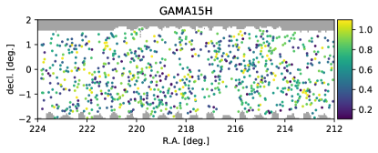
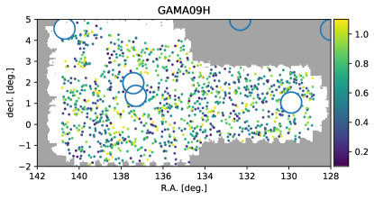
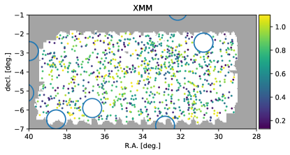
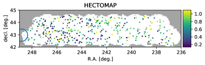
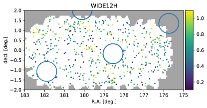
Figure 1: The sky distribution of the CAMIRA clusters for 6 patches used in this work. Points show centre positions of the clusters and colour level represents cluster’s redshift. Circles are masked regions with radii of $0.5^{\circ}$ from point-source centre (also see Section 2.3). In shaded regions, the clusters are not identified either because there is no observation or the data is shallow.

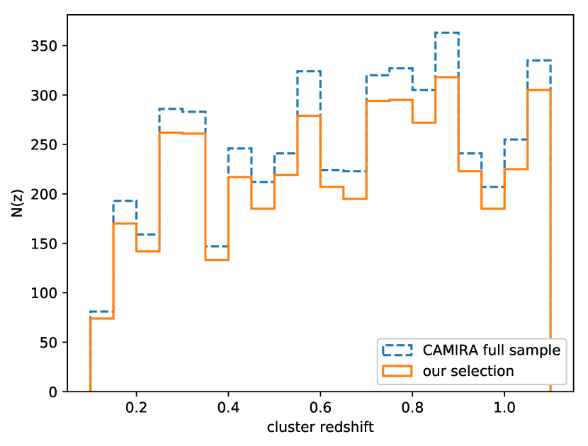
Figure 2: The redshift distribution of CAMIRA clusters in HSC S16A. The comparison with the full sample suggests that our sample selection due to the edge and point mask does not significantly bias the distribution.

2.2 Fermi-LAT data reduction

The $\gamma$-ray analysis pipeline proceeds similarly to what is described in Shirasaki et al. (2018a), and we refer the reader to that work for further details. In summary, we analyse $\sim 7$ years (from August 4, 2008 to September 4, 2015) of Pass 8 ULTRACLEANVETO photons and select $\gamma$-ray events in the energy range $E=[1,100]$ GeV. We impose standard selection cuts on the $\gamma$-ray data, removing events entering at zenith angles larger than 90^∘ to reduce cosmic-ray contamination. Moreover, the photon data was filtered by removing time periods when the instrument was not in sky-survey mode. To produce flux maps in our regions of interest (ROI) we use the Fermi Science Tools v10r0p5 software package and the instrument response functions (IRFs), P8R2_ULTRACLEANVETO_V6.

As described in Appendix A of Shirasaki et al. (2018a), we analyse $\gamma$-rays within square regions of size $20^{\circ}\times 20^{\circ}$ around each of the HSC fields of view. To reduce the computation time of our pipeline in the ROIs we further divided each $20^{\circ}\times 20^{\circ}$ region into four $12^{\circ}\times 12^{\circ}$ contiguous patches with overlapping boundaries. The measured $\gamma$-rays at each patch were modeled by a linear combination of diffuse $\gamma$-ray background and foreground models as well as lists of $\gamma$-ray point sources present in the ROIs.

In particular, we employ two different kinds of interstellar emission models (IEMs) in order to estimate the systematic uncertainties introduced by the choice of IEM. The first IEM, included in our baseline model, corresponds to the standard LAT diffuse emission model, gll_iem_v06.fits, this is the model routinely used in Pass 8 analyses. As alternative IEMs, we consider three different diffuse models produced with the GALPROP cosmic-ray propagation code. These alternative IEMs (called Models A, B and C) were introduced in Ackermann et al. (2015) and encompass a very wide range of the systematics associated with this kind of analysis. As such, they provide a test in rigor comparable to that performed by the Fermi team.

The fit started with a sky model that includes all point-like and extended LAT sources listed in the 3FGL (Acero et al. 2015) catalogue as well as a list of new point sources found in Shirasaki et al. (2018a) (see Table III in the appendix section). In our baseline model the Galactic diffuse emission was modeled by the standard LAT diffuse emission model, and as a proxy for the residual background and extragalactic $\gamma$-ray radiation we used the isotropic template given by model, iso_P8R2_ULTRACLEANVETO_V6_v06.txt. Best-fit spectral parameters were obtained for all free sources within our $12^{\circ}\times 12^{\circ}$ ROIs. To obtain convergence, all the fits were performed hierarchically; freeing first the normalization of the sources with the highest intensities followed by the lower ones within the ROIs. The fitting consecutively restarts from the updated best-fit models and repeats the same procedure this time for the spectral shape parameters.

The EGB in the ROIs were obtained by subtracting the best-fit Galactic diffuse emission model from the photon counts maps. We note that the EGB images obtained in this way could still contain some isotropic detector backgrounds. However, our analysis is able to reproduce well the EGB $\gamma$-rays derived by the Fermi-LAT team (see, e.g. Ref. Shirasaki et al. (2016) for an example of this method). This shows that most of the detector cosmic-ray induced backgrounds are safely removed by our conservative photon selection filters.

2.3 UGRB map

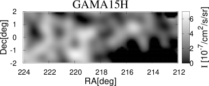
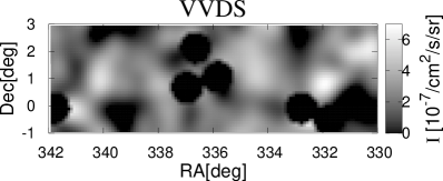
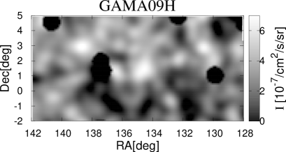
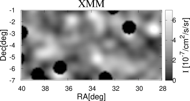
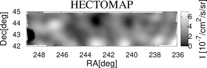
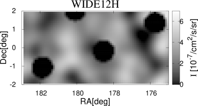
Figure 3: UGRB maps corresponding to CAMIRA-cluster regions (Figure 1) in our analysis. The colour bar is an amplitude of the number intensity for $\gamma$-ray photons. In this figure, the UGRB maps are constructed from Fermi $\gamma$-ray data of 1-100 GeV by masking point-source regions (circular black shaded areas), subtracting the Galactic $\gamma$-ray emission for the baseline model and applying a Gaussian smoothing of $0.5^{\circ}$. Note that only in this figure, we do not only apply a smoothing scale of $0.5^{\circ}$ below 10 GeV but also higher than 10 GeV.

In our analysis, we use the Fermi $\gamma$-ray data of 1-100 GeV. To subtract the diffuse Galactic $\gamma$-ray emission, four foreground models are applied: baseline model, Model A, B, and C (Ackermann et al. 2015). The mean number intensities of the $\gamma$-ray photons for the UGRB applied each foreground model are 2.57, 2.04, 2.24 and 2.45$~{}(10^{-7}{\rm cm^{-2}s^{-1}sr^{-1}})$ for baseline model, Model A, B and C, respectively. We also subtract emission from resolved point sources listed in the 3FGL catalogue (Acero et al. 2015) and new point-source candidates (Shirasaki et al. 2018b). To be more conservative, we mask circular regions of radius $0.5^{\circ}$ around the point sources to avoid a possible overcorrection for the $\gamma$-ray fluxes.

Since the mean number intensity of $\gamma$-ray per pixel is small, $\sim 0.1$, we apply a Gaussian smoothing filter on the UGRB map to relax the shot noise effect. The smoothing scales depend on the energy of $\gamma$-ray observed and we take 0.5^∘ for below $10{\rm GeV}$, and 0.2^∘ otherwise, which roughly correspond to the size of PSF, which again depends on the energy scale of $\gamma$-ray (Ackermann et al. 2012a). Figure 3 shows the processed $\gamma$-ray map in six different fields where all the $\gamma$-ray photon is integrated over 1-100 GeV.

3 STACKING ANALYSIS

In this section, we perform the stacking analysis between the UGRB map and CAMIRA clusters. The stacking analysis is useful to visually find a correlation signal and is basically equivalent to the cross-correlation analysis which we describe in section 4. This analysis can increase a signal-to-noise (SN) ratio by combining multiple images. In this section, we describe the method of stacking analysis and show the result.

First we select a $4^{\circ}\times 4^{\circ}$ square image of the UGRB, centred at each cluster position, which is defined as the location of the most probable BCG among the member galaxies(Oguri et al. 2018). After randomly rotating the images, we stack all images to obtain the average image of $\gamma$-ray around the cluster, we call it as stacked image at “cluster”,

$$I_{\rm stack}^{\rm clu}(\mbox{\boldmath$\theta$})=\frac{1}{N_{\rm clu}\overline{I_{\gamma}}}\sum_{i}^{\rm N_{clu}}{\mathcal{G}}(\mbox{\boldmath$\phi$}_{i})I_{\gamma}(\mbox{\boldmath$\Theta$}_{i}-\mbox{\boldmath$\Theta$}_{i,\rm clu}),$$ (1)

where $\theta$ is a separation angle from cluster centre, $N_{\rm clu}$ is the number of clusters to be stacked, $I_{\gamma,i}(\mbox{\boldmath$\Theta$}_{i}-\mbox{\boldmath$\Theta$}_{i,\rm clu})$ is the number intensity of $\gamma$-ray for around the $i$-th cluster centred at $\mbox{\boldmath$\Theta$}_{i,\rm clu}$ and $\overline{I_{\gamma}}$ is the averaged $I_{\gamma}$ over all ROIs. The rotation operator ${\mathcal{G}}$ is defined in the local coordinate and its argument $\mbox{\boldmath$\phi$}_{i}$ is randomly selected from $[0,2\pi]$. The random rotation of each map can reduce the effect of large scale anisotropies due to the imperfect subtraction of Galactic foreground component.

The stacked image at “cluster” might include not only the $\gamma$-ray light from clusters identified in the CAMIRA catalogue but also the background or foreground $\gamma$-ray not associated to the clusters. To subtract any components not related to clusters from the stacked image, we also make random stacked images through the similar procedure, in which we select random positions as the centre of the images for stacking, instead of the CAMIRA cluster position: i.e. by replacing the superscript of “clu” with “ran” in equation (1). Then, we obtain the final stacked $\gamma$-ray image by subtracting the “random” image from the “cluster” one.

$$\delta_{\rm stack}(\mbox{\boldmath$\theta$})=I_{\rm stack}^{\rm clu}(\mbox{\boldmath$\theta$})-I_{\rm stack}^{\rm ran}(\mbox{\boldmath$\theta$})$$ (2)

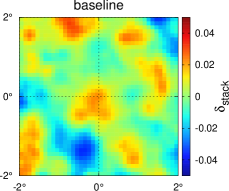
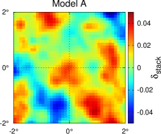
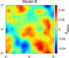
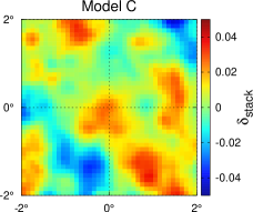
Figure 4: Stacked maps using the UGRB map for different Galactic foreground models. The colour bar is an amplitude of stacked fluctuation for the $\gamma$-ray number intensity. Cluster centre is located at $(0^{\circ},0^{\circ})$.

Figure 4 shows the final stacked image for different Galactic foreground models. One can clearly see the $\gamma$-ray excess at the centre region. This excess corresponds to a few per cent of the average intensity and extends to $\sim 1^{\circ}$ which corresponds to about a few 10 Mpc, for typical CAMIRA cluster’s redshift, $z\sim 0.6$. This is clearly larger than the typical size of cluster. We repeat the same analysis but limited $\gamma$-ray samples at lower energy bins, that is $<5$ GeV, the result is not changed dramatically. This means that the signal at the central region is dominated by the lower energy $\gamma$-ray photons. As we see in Section 2.3, the PSF size depends on the $\gamma$-ray energy and thus this widely spread diffusion signature can be due to the PSF of the Fermi-LAT, however; we do not exclude any possibilities that this diffusive signature originates from the cluster vicinity regions, like filaments or wall. We also see in figure 4 that the contrast of the intensity slightly depends on the foreground model, which infers the Galactic foreground models includes uncertainties at the level of the difference of the signal at central region among different models.

We repeat the above analysis for subsamples of clusters divided in two redshift ranges, $0.1<z<0.6$ and $0.6<z<1.1$, which is shown in Figure 5. For the low-redshift cluster, a strong correlation is found around the clusters position. Moreover, the signal is spatially distributed more widely around the centre than in the case of all clusters shown in Figure 4. On the other hand, for the higher-redshift cluster, we only see a slight excesses at the centre. We note however that signal to noise ratios for the stacked map are $\sim 1$. Therefore, the stacked map has a comparable level of noise to the signal and the strong pattern of the map is likely due to the noise. And also note that each $4^{\circ}\times 4^{\circ}$ image used for the stacking analysis is highly correlated with one another. The average separation of the CAMIRA clusters is $\sim 0.22~{}$degree and is much smaller than the image size of $\sim 4$ degrees). Therefore, some photons appear multiple times at different positions in the “stacked” image. For this reason, we do not conduct a quantitative discussion using the “stacked” image. Instead, we perform the the cross-correlation analysis in the next section.

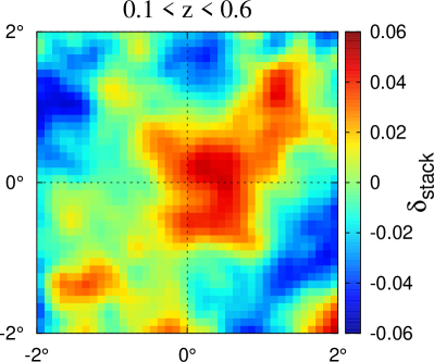
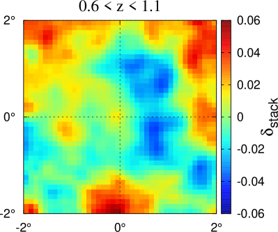
Figure 5: Same as upper left panel of Figure 4, but for clusters at $0.1<z<0.6$ (Left) and $0.6<z<1.1$ (Right).

4 CROSS-CORRELATION ANALYSIS

In this section, we perform the cross-correlation analysis between CAMIRA clusters and the UGRB map. We describe our method for the evaluation of the cross-correlation between them and then show the results.

4.1 correlation function

To evaluate the two-point cross-correlation function, we use the Landy-Szalay estimator (Landy & Szalay 1993). Kerscher et al. (2000) have shown that the Landy-Szalay estimator provides the most accurate result compared with other estimators. The Landy-Szalay estimator $\xi_{\rm obs}(\theta)$ is given as a function of a separation angular scale $\theta$ through

$$\xi_{\rm obs}(\theta)=\frac{n^{D}_{\rm clu}I^{D}_{\gamma}-n^{D}_{\rm clu}I^{R}_{\gamma}-n^{R}_{\rm clu}I^{D}_{\gamma}+n^{R}_{\rm clu}I^{R}_{\gamma}}{n^{R}_{\rm clu}I^{R}_{\gamma}},$$ (3)

where $n_{\rm clu}=n_{\rm clu}(\mbox{\boldmath$\theta$}_{1})$ is the number of clusters at a cluster position, $\mbox{\boldmath$\theta$}_{1}$. $I_{\gamma}=I_{\gamma}(\mbox{\boldmath$\theta$}_{2})$ is the number intensity of $\gamma$-ray at $\mbox{\boldmath$\theta$}_{2}$ where $|\mbox{\boldmath$\theta$}_{1}-\mbox{\boldmath$\theta$}_{2}|=\theta$. The superscripts $D$ and $R$ represent the actual data (i.e. the CAMIRA cluster number count and the UGRB intensity) and the random data. We use the random CAMIRA catalogue containing 185,459 clusters as random data of the CAMIRA cluster number count. The random CAMIRA catalogue is made by running the CAMIRA for randomly distributed mock samples of galaxies within the same fields as data. For the random map of the UGRB, we generate the random intensity map assuming photon obeys a Poisson distribution with total number of photons being one hundred times larger than what observed.

4.2 covariance

To evaluate the error on the cross-correlation estimator, we use the jackknife method (Scranton et al. 2002). Here we divide both CAMIRA catalogue and the UGRB map into 21 subregions. Individual subregion spans $3.5\times 3.5$[deg²] area on average, which is sufficiently larger than the scale of interest. The covariance matrix is then given by

$${\bf C}_{ij}=\frac{M-1}{M}\sum^{M}_{k=1}\left[\widehat{\xi_{k}(\theta_{i})}-\overline{\xi(\theta_{i})}\right]\times\left[\widehat{\xi_{k}(\theta_{j})}-\overline{\xi(\theta_{j})}\right],$$ (4)

where $M$ is the number of the jackknife subsamples, $M=21$ in our case, and $\widehat{\xi_{k}(\theta)}$ is the correlation function for the $k$-th jackknife re-sample where we remove the $k$-th subregion from the entire region. Mean correlation function is obtained by averaging over all different jackknife re-samples,

$$\overline{\xi(\theta)}=\frac{1}{M}\sum_{k}^{M}\widehat{\xi_{k}(\theta)}$$ (5)

In Figure 6, we show the profiles of the cross-correlations for clusters in all redshifts, low redshifts ($z<0.6$) and high redshifts ($z>0.6$). One can clearly see the cross-correlation signals within $\sim 1$ degree, for the all-redshift clusters and the low-redshift cases. The signals for low-redshift clusters extend wider than those for all clusters. The excess at the cluster position is independent on the Galactic foreground model. Contrarily, the cross-correlation signals for high-redshift clusters are rather weak. In particular, with the baseline model, it seems that the signal is consistent with zero. The difference among the different foreground models is within the one-sigma error bars. Therefore, with the current data sets of the high-redshift clusters, we cannot conclude the detection or non-detection of the cross-correlation signal and cannot make a further discussions on the dependence of the signal on the Galactic foreground models. Note that as we will describe in 4.3, there are strong correlations among different angular bins. Also note that the error estimation of the jackknife method sometimes brings misestimation but it is quite hard to perform full simulation of $\gamma$-ray diffuse sky as we do not understand the origin of the diffuse emission. Those treatments are beyond the scope of this paper and we emphasise that the results are all based on the error estimation from the jackknife method.

4.3 Detection

Here we estimate the statistical significance of the signal for all-redshift, low-redshift and high-redshift galaxy cluster sets. To evaluate the significance we adopt the standard $\chi^{2}$ statistics with the null hypothesis taking into account a possible correlation among different angular bins,

$$\chi^{2}_{\rm mod}=\sum_{i,j}\left[\overline{\xi(\theta_{i})}-\xi_{\rm mod}(\theta_{i})\right]\widetilde{\bf C}^{-1}_{ij}\left[\overline{\xi(\theta_{j})}-\xi_{\rm mod}(\theta_{j})\right],$$ (6)

where $\xi_{\rm mod}(\theta)$ is a hypothetical prediction for the cross-correlation function, which meanwhile we assume to be zero to find the detection significance and is later given in Section 5 to compare the signal with the theoretically predicted model. The matrix $\widetilde{\bf C}^{-1}$ is a pseudo-inverse of the covariance matrix. As can be seen in Figure 7, there are significant correlations between different angular scales. In general, if there is a strong correlation, the matrix inversion is noisy. To regularize the matrix, we apply a singular value decomposition (SVD) to obtain the pseudo-inverse of the covariance matrix, which is numerically stable. The covariance matrix can be decomposed as

$${\bf C}={\bf u}~{}\mbox{\boldmath$\Sigma$}~{}{\bf v}^{\rm T},$$ (7)

where $\Sigma$ is a diagonal matrix which consists of eigenvalues of the covariance matrix $\lambda_{i}$ arranged in a descending order. We then remove the eigenvalues small enough compared to the largest eigenvalue, which makes inversion noisy. By looking at the numerical convergence, we decide largest four eigenvalues are meaningful and others are not informative. Then the pseudo inverse matrix is given as

$$\widetilde{\bf C}^{-1}={\bf v}~{}\mbox{\boldmath$\Sigma$}^{\prime-1}~{}{\bf u}^{\rm T},$$ (8)

where

$$\mbox{\boldmath$\Sigma$}^{\prime-1}={\rm diag}\left(\frac{1}{\lambda}_{1},\cdots,\frac{1}{\lambda}_{k},0,\cdots,0\right),$$ (9)

and $\lambda_{i}$ are the eigenvalues of covariance matrix satisfying $\lambda_{i}>\lambda_{i+1}$ for all $i$. The smallest eigenvalue which is not negligible is $\lambda_{k}$.

The detection significance which is summarised in Table 1 can be obtained by setting $\xi_{\rm mod}(\theta_{i})=0$ in Eq (6), assuming the probability function obeys Gaussian distribution. We find that the cross-correlation signal is around $2\sigma$ or smaller, which means the marginal evidence for the $\gamma$-ray association to the cluster of galaxies. In addition, the significance fluctuates depending on the foreground model we assumed and thus the detection significance is rather weak.

We note that although it is empirically known that for $10\times 10$ covariance, it is required to have 100 jackknife subregions. However, in our dataset, due to the limited survey area of HSC and the scale of our interest which extends up to 2 degrees, it is difficult to patch the sky into 100 subregions. Therefore, we revisit the analysis to derive the significance with coarser binning of $4\times 4$ covariance, which can be well measured by 21 jackknife sampling. We find that the obtained significance is different only by less than 10 per cent from those for 10 binning, which implies that our measurement of $10\times 10$ covariance with 21 subsampling would be reasonable.

As we described in section 2.1, we have used the cluster catalogue aggressively, $\hat{N}_{\rm mem}>10$; however, it may contain some fake clusters due to the projection effect. In order to see the robustness of our analysis, we repeat our analysis for the sample $\hat{N}_{\rm mem}>15$. For the sample $\hat{N}_{\rm mem}>15$, we find smaller amplitude of cross correlation at low-z and larger at high-z; however, they are still consistent with each other within 1$\sigma$ error bars. The subtle mass and redshift dependencies of the signal imply that the CAMIRA clusters likely contaminated by the fake clusters at high-redshift especially at less massive end so that our signal for $\hat{N}_{\rm mem}>10$ are more contaminated by the fake clusters, while it is less affected by the fakes at low-redshift.

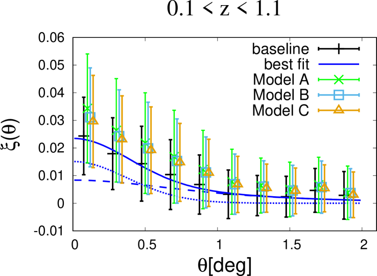
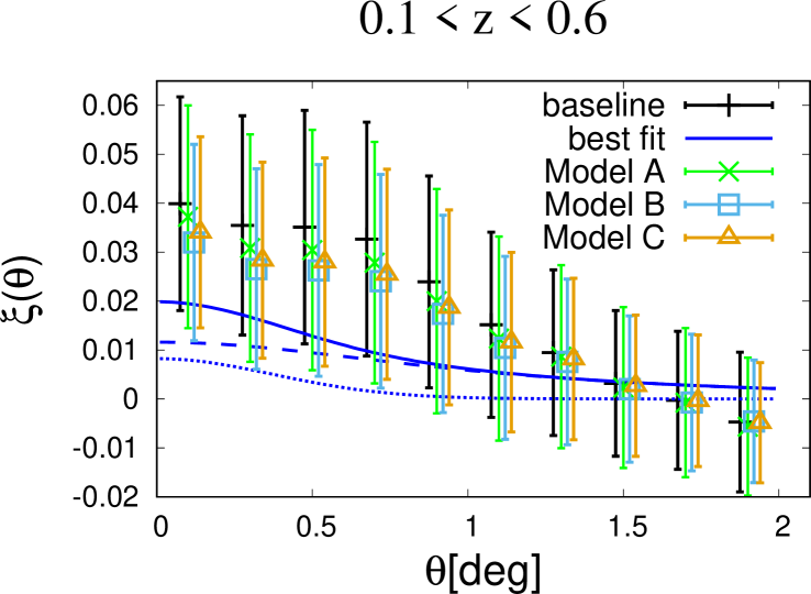
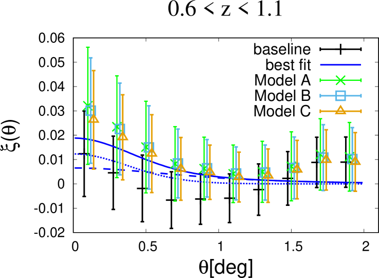
Figure 6: Cross correlation signal of $\gamma$-ray map and cluster distribution for all-(top) , low redshift-(middle) and high redshift-(bottom) clusters, respectively. Symbols with error bars are measured angular cross correlation with different symbols correspond to different foreground models. Solid lines are best-fitted theoretical predictions to the data corrected with the baseline foreground model. The theoretical model can be decomposed into to components: astronomical objects such as blazars, star-forming galaxies and radio galaxies (dashed) and shot noise term (dotted). For more details about the theoretical prediction, refer to the text in section 5.

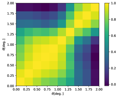
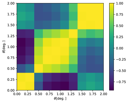
Figure 7: (Left) Covariance matrix of cross correlation for the base-line foreground model, normalised by diagonal terms, ${\rm C}_{ij}/\sqrt{{\rm C}_{ii}{\rm C}_{jj}}$. Off diagonal terms are not negligible which mean a significant correlation among different angular scales. (Right) Pseudo-inverse of the covariance matrix remaining largest four eigenvalues (see text for details), normalised again by diagonal terms.

redshift range	baseline	Model A	Model B	Model C
$0.1~{}<~{}z~{}<~{}1.1$	2.2	2.0	2.0	2.0
$0.1~{}<~{}z~{}<~{}0.6$	2.2	2.1	2.1	2.3
$0.6~{}<~{}z~{}<~{}1.1$	1.9	1.6	1.6	1.6

Table 1: Statistical significances for detecting the cross correlation with different Galactic foreground models and redshift ranges of clusters. Note that we use 1942 low-redshift clusters and 2519 high-redshift clusters.

5 Implication

The UGRB is expected to be cumulative $\gamma$-ray emissions from unresolved extragalactic sources as well as some diffuse processes. Blazars are one of the most abundant point sources in GeV $\gamma$-ray energy and known to be a main contributor to extragalactic $\gamma$-ray emissions. The latest model of $\gamma$-ray spectrum and luminosity function of blazars can naturally explain about 70 per cent of the extragalactic $\gamma$-ray intensity above 1 GeV (e.g. Ajello et al. 2015). Other possible candidates contributing to UGRB include star forming galaxies (e.g. Thompson et al. 2007) and radio galaxies (e.g. Inoue 2011). Here, we consider a simple model of cross correlation assuming that blazars, star-forming galaxies, and radio galaxies are biased tracers of large-scale structures in the Universe.

The UGRB intensity along a given direction $\theta$ can be written as

$$I_{\gamma}(\mbox{\boldmath$\theta$})=\sum_{X}\int{\rm d}\chi\,W_{\gamma,X}(\chi)\,g_{X}(r(\chi)\mbox{\boldmath$\theta$},\chi),$$ (10)

where $\chi(z)$ denotes the radial comoving distance (function of redshift $z$), $r(\chi)$ is the comoving angular diameter distance, $W_{\gamma,X}(\chi)$ is the window function for population $X$, and $g_{X}(\mbox{\boldmath$x$})$ is the relevant density field of the $\gamma$-ray source $X$. We here define $W_{\gamma,X}(\chi)$ so that the mean $\gamma$-ray intensity can be expressed as $\sum_{X}\,\int{\rm d}\chi\,W_{\gamma,X}(\chi)$. We compute the window function $W_{\gamma,X}$ as follows in Shirasaki et al. (2018a). The model includes $\gamma$-ray luminosity function and energy spectrum for different source populations and $\gamma$-ray attenuation during propagation owing to pair creation on diffuse extragalactic photons (Gilmore et al. 2012). For blazars, we consider a parametric description of $\gamma$-ray luminosity function and energy spectrum as developed in Ajello et al. (2015). For star-forming galaxies, we assume a correlation of luminosity between $\gamma$ ray and infrared to derive their $\gamma$-ray luminosity function (Ackermann et al. 2012b). The energy spectrum of star-forming galaxies is set to be $E^{-2.2}$ (Ackermann et al. 2012b). For radio galaxies, we follow the model in Di Mauro et al. (2014), which has established a correlation between the $\gamma$-ray luminosity and the radio-core luminosity at 5 GHz. We assume an average spectral index of 2.37 for radio galaxies. To define the “unresolved” components for population $X$, we set the $\gamma$-ray flux limit of $2\times 10^{-9}\,{\rm cm}^{-2}\,{\rm s}^{-1}$ above 100 MeV.

The angular number density field of CAMIRA clusters can be expressed as

$$n_{\rm clu}(\mbox{\boldmath$\theta$})=\int{\rm d}\chi\,\chi^{2}\int{\rm d}M\,S\left(M,z\left(\chi\right)\right)\,$$

$$\hskip 90.00014pt\times\bar{n}\left(M,z\left(\chi\right)\right)\left[1+\delta_{h}(\chi\mbox{\boldmath$\theta$},\chi)\right],$$ (11)

where $\bar{n}(M,z)$ represents the halo mass function, $S(M,z)$ is the selection function for CAMIRA clusters, and $\delta_{h}(\mbox{\boldmath$x$})$ is the overdensity field of three-dimensional halo number density. As in Section 2.1, we assume $S=1$ for $M\geq 10^{13.5}\,h^{-1}\,M_{\odot}$ and $S=0$ otherwise in this paper. We adopt the model of $\bar{n}$ as in Tinker et al. (2008) for the spherical overdensity parameter $\Delta=200$ with respect to mean cosmic matter density. Under a flat-sky approximation, we can express the cross correlation between $n_{\rm clu}$ and $I_{\gamma}$ in Fourier space as (also see Branchini et al. 2017),

$$P_{{\rm c}\gamma}(\ell)=\sum_{X}\int\frac{{\rm d}\chi}{r(\chi)^{2}}\,W_{\gamma,X}(\chi)\,W_{\rm clu}(\chi)\,P^{(\rm 3D)}_{{\rm h}X}\left(\frac{\ell}{r(\chi)},z(\chi)\right),$$ (12)

where $\ell$ is the multipole and $P^{(\rm 3D)}_{{\rm h}X}$ represents the three-dimensional cross power spectrum between $g_{\gamma,X}$ and $\delta_{h}$ (see Eqs. (10) and (11)). In Eq. (12), we define the effective window function for CAMIRA clusters as

$$W_{\rm clu}(\chi)\equiv\chi^{2}\int{\rm d}M\,S\left(M,z\left(\chi\right)\right)\,\bar{n}\left(M,z\left(\chi\right)\right).$$ (13)

On degree scales, linear approximation of the evolution in two fields $g_{\gamma,X}$ and $\delta_{h}$ will be valid. In contrast, we expect the shot noise term arising from the finite sampling of CAMIRA clusters and unresolved $\gamma$-ray sources for small scales. In this case, the three-dimensional power spectrum can be approximated as $P^{(\rm 3D)}_{{\rm h}X}(k,z)=\bar{b}_{\rm h}(z)\bar{b}_{{\rm eff},X}(z)P_{\rm L}(k,z)+{\cal A}$, where $P_{\rm L}(k,z)$ represents the linear matter power spectrum at redshift $z$, $\bar{b}_{\rm h}$ is the linear halo bias including the selection effect in halo mass, $\bar{b}_{{\rm eff},X}$ is the effective bias factor of $\gamma$-ray population $X$, and ${\cal A}$ is the shot noise term. In this paper, we compute $\bar{b}_{\rm h}$ as

$$\bar{b}_{\rm h}(z)=\frac{\int{\rm d}M\,S(M,z)\,\bar{n}(M,z)\,b(M,z)}{\int{\rm d}M\,S(M,z)\,\bar{n}(M,z)},$$ (14)

where $b$ is the linear bias and we adopt the model of $b$ in Tinker et al. (2010). Unfortunately $\bar{b}_{{\rm eff},X}$ is still uncertain and it should be constrained by clustering analyses of gamma rays with large-scale structures in practice. For simplicity, we adopt the fiducial model of $\bar{b}_{{\rm eff},X}$ in Shirasaki et al. (2018a). We leave possible constraints of $\bar{b}_{{\rm eff},X}$ by our measurements for our future work. It is also worth mentioning that there exist other possible sources to generate the cross correlation. They include the $\gamma$-ray emissions from intra-cluster medium (e.g. Colafrancesco & Blasi 1998) and dark matter annihilations (e.g. Jungman et al. 1996). Our measurement can be useful to constrain these possible $\gamma$-ray emissions and we plan to explore them in the future.

Our observable $\xi$ is related with $P_{{\rm c}\gamma}(\ell)$ through Fourier transform:

$$\xi(\theta)=\frac{1}{\langle n_{\rm clu}\rangle\langle I_{\gamma}\rangle}\int\frac{{\rm d}^{2}\ell}{(2\pi)^{2}}\,\exp\left[i\mbox{\boldmath$\ell$}\cdot\mbox{\boldmath$\theta$}\right]\,P_{{\rm c}\gamma}(\ell)\hat{W}(\ell,\theta_{G}),$$ (15)

where $\langle\cdots\rangle$ represents the average over a sky and $\hat{W}$ is the Fourier counterpart of two-dimensional Gaussian smoothing filter with the smoothing scale of $\theta_{G}$. Although Eq. (12) does not include the smearing effect by $\gamma$-ray point spread function (PSF), we include the effect by convolving the $W_{\gamma,X}$ with the $\gamma$-ray PSF when comparing our prediction with observation (see Shirasaki et al. 2014, for details). In summary, our model of $\xi$ has single free parameter $\cal A$, while we fix the cross correlation coming from large-scale clustering between CAMIRA clusters and $\gamma$-ray sources.

Blue solid lines in figure 6 show the best-fit model of cross correlation. We define the best-fit model to minimise the chi-squared value as in Eq. (6) by varying the parameter. We find our simple model with single free parameter can reasonably explain the observed correlation regardless of selections in cluster redshift. Systematic effects due to imperfect modeling of Galactic $\gamma$-ray foreground are found to be unimportant for the current analysis. The minimum chi-squared values and the number intensity of the shot noise term giving the minimum $\chi^{2}_{\rm mod}$ in our analysis are summarised in Table 2 and Table 3, respectively. In the case of low-redshift clusters, astronomical sources contribute largely for the correlation and the shot noise term has a weaker effect. In contrast, in the case of all clusters or high-redshift clusters, the shot noise term is dominant for model prediction on small scale ($<\sim 0.5^{\circ}$). We note that the best-fitting amplitudes of the shot noise term are larger than the ones in Branchini et al. (2017) by a factor of 10 ;however, due to the large uncertainties, it is still consistent within $1\sigma$ errors. We also note that the theoretical model includes uncertainties for $\gamma$-ray sources and a bias parameter $b_{\rm eff}$.

Due to the small number of samples for the $\gamma$-ray sources, it is yet difficult to discuss the effect of flux uncertainties on the model prediction but according to the current limited samples, the uncertainties on the $\gamma$-ray sources ranges from 0.2 to 2 (Ajello et al. 2015; Ackermann et al. 2012b; Inoue 2011). The model for the bias also includes large uncertainties; we have no reliable Halo Occupation Distribution model for blazars yet. Allevato et al. (2014) measured angular correlation of BL Lacs and flat-spectrum radio quasars and found that the linear biases for them are $1.84\pm 0.25$ and $3.30\pm 0.41$, respectively. From this study, we can infer the magnitude of the bias uncertainty is about 50 per cent.

Since the angular resolution in Fermi UGRB is of an order of degree, the effective number of degrees of freedom can be smaller than figure 6 actually shows. To investigate the nature of UGRB with our cross-correlation function in details, the cross correlation measurement in Fourier space will be essential and we will work on Fourier-space analysis in the future.

redshift range	Baseline	Model A	Model B	Model C
$0.1~{}<z<~{}1.1$	0.30	0.29	0.28	0.27
$0.1~{}<z<~{}0.6$	2.2	1.9	1.8	2.2
$0.6~{}<z<~{}1.1$	2.5	0.79	0.76	0.78

Table 2: The minimum chi-squared values in our comparison with model and observed correlation $\chi^{2}_{\rm mod}$. We summarise the results for three different cluster redshift ranges for different Galactic foreground models. Note that effective number of degree-of-freedom is 3 for all cases.

redshift range	Baseline	Model A	Model B	Model C
$0.1~{}<z<~{}1.1$	5.1	6.3	5.6	5.2
$0.1~{}<z<~{}0.6$	2.8	4.4	3.6	3.6
$0.6~{}<z<~{}1.1$	4.2	6.9	6.3	5.6

Table 3: The best fit value for the amplitude of the shot noise term ($10^{-9}{\rm cm^{-2}s^{-1}sr^{-1}}$).

6 Summary

In this paper, we have investigated the cross-correlation signal between the UGRB, the PASS8 Fermi-LAT data, and the HSC galaxy clusters, the CAMIRA cluster catalogue. To evaluate the cross-correlation signals, we have performed both the stacking analysis and the cross-correlation analysis. We have evaluated the cross-correlation signal quantitatively by the cross-correlation analysis, while the stacking analysis is used to confirm the validity of the cross-correlation analysis.

In both analyses, we have found evidence of the cross-correlation signal. The signal appears as a few per cent excess of the photon number intensity to the background. Although we have adopted four models of the Galactic diffuse emission to subtract the foreground contamination, the signal does not depend on the foreground model. The statistical significance of the signal detection reaches 2.0-2.3$\sigma$ significance independently of any of our Galactic foreground models.

The cross-correlation analysis has shown that the signal extends up to $\sim 1^{\circ}$ from cluster centres. This angular scale corresponds to $5{\rm Mpc}/h$ (at $z=0.1$) to $40{\rm Mpc}/h$ (at $z=1.1$) which is well beyond the typical scale of cluster. The size of PSF for the Fermi-LAT data varies from $0.1^{\circ}$ to $1^{\circ}$ for 100 GeV to 1 GeV and we find that our cross correlation signal is fully dominated by the lower energy photons (1-5 GeV). Therefore, we conclude that while the extension of signal is mainly dominated by the PSF of the $\gamma$-ray photons, we may not exclude the possibility that this signal extension is due to the over-densities around cluster regions (e.g. Branchini et al. 2017).

We have also studied the redshift dependence of the cross-correlation signal, by dividing the cluster catalogue into two redshift bins, low-redshift clusters $(0.1<z<0.6)$ and high-redshift clusters $(0.6<z<1.1)$. We have found that the cross-correlation signal with low-redshift sample is stronger than that with the high-redshift sample. The detection significances are $2.1-2.3\sigma$, $1.6-1.9\sigma$, and $2.0-2.2\sigma$ for low-redshift, high-redshift, and all-redshift samples, respectively. With our current dataset, we do not claim a significant detection of the cross correlation between $\gamma$-ray sources and cluster of galaxies, given that the statistical significance fluctuates depending on the foreground model we assumed.

We see that the signals for only $\hat{N}_{\rm mem}>15$ are still consistent with all samples of $\hat{N}_{\rm mem}>10$ and the obtained significance is not largely affected by this choice of the minimum mass of the clusters.

To study the source of the cross-correlation signal, we have compared the measured cross-correlation function with a theoretical model. The model includes the contributions from blazars, star-forming galaxies and radio galaxies as $\gamma$-ray emitters in a cluster. It seems that the detected signal is fairly consistent with the theoretically predicted model. We leave a more detailed modeling of the astronomical origins of the $\gamma$-ray emitters as well as the exploration to the light from dark matter for future work.

In this analysis, we used $\sim 4000$ clusters from the current HSC CAMIRA cluster catalogue and $\sim 200~{}{\rm deg}^{2}$ UGRB map (the number of $\gamma$-ray photons is $\sim 3000$). We repeat the same analysis for half of our survey region and find that the error scales by a factor of $\sqrt{2}$, which means the error is fully explained by the cosmic variance. As more data is accumulated, our detected signal can become more robust with smaller error bars in the future. For example, the number of CAMIRA clusters is expected to increase as the HSC observation area will increase by at least three times, the statistical error can be reduced by a factor of $1/\sqrt{3}$. If the same signal appears in future data, the significances of the such correlation signals will be improved to $3\sigma$ levels even for high-redshift clusters. The accumulation of the data in both galaxy clusters and $\gamma$-ray photons will allow us to perform further statistical analysis including the one with multiple redshifts or energy binnings. Such analyses may not only reveal more details of the cross-correlation of the UGRB with clusters but also constrain the nature of dark matter as a source of $\gamma$-rays through their annihilations, decays or radiation as primordial black-holes evaporation.

References

- Acero et al. (2015) Acero F. et al., 2015, ApJS, 218, 23
- Acero et al. (2015) Acero F., et al., 2015, Astrophys. J. Suppl., 218, 23
- Ackermann et al. (2012a) Ackermann M. et al., 2012a, ApJS, 203, 4
- Ackermann et al. (2016) Ackermann M. et al., 2016, ApJ, 819, 149
- Ackermann et al. (2015) Ackermann M. et al., 2015, ApJ, 799, 86
- Ackermann et al. (2012b) Ackermann M. et al., 2012b, ¥apj, 755, 164
- Aihara et al. (2018a) Aihara H. et al., 2018a, PASJ, 70, S4
- Aihara et al. (2018b) Aihara H. et al., 2018b, PASJ, 70, S8
- Ajello et al. (2015) Ajello M. et al., 2015, ApJ, 800, L27
- Allevato et al. (2014) Allevato V., Finoguenov A., Cappelluti N., 2014, ApJ, 797, 96
- Ando (2014) Ando S., 2014, JCAP, 10, 061
- Ando et al. (2017) Ando S., Fornasa M., Fornengo N., Regis M., Zechlin H.-S., 2017, Phys. Rev. D, 95, 123006
- Ando & Komatsu (2006) Ando S., Komatsu E., 2006, Phys. Rev. D, 73, 023521
- Ando & Komatsu (2013) Ando S., Komatsu E., 2013, Phys. Rev. D, 87, 123539
- Atwood et al. (2009) Atwood W. B. et al., 2009, ApJ, 697, 1071
- Axelrod et al. (2010) Axelrod T., Kantor J., Lupton R. H., Pierfederici F., 2010, in Proc. of SPIE, Vol. 7740, Software and Cyberinfrastructure for Astronomy, p. 774015
- Bosch et al. (2018) Bosch J. et al., 2018, PASJ, 70, S5
- Branchini et al. (2017) Branchini E., Camera S., Cuoco A., Fornengo N., Regis M., Viel M., Xia J.-Q., 2017, ApJS, 228, 8
- Bruzual & Charlot (2003) Bruzual G., Charlot S., 2003, MNRAS, 344, 1000
- Camera et al. (2015) Camera S., Fornasa M., Fornengo N., Regis M., 2015, JCAP, 6, 029
- Carr et al. (2010) Carr B. J., Kohri K., Sendouda Y., Yokoyama J., 2010, Phys. Rev. D, 81, 104019
- Colafrancesco & Blasi (1998) Colafrancesco S., Blasi P., 1998, Astroparticle Physics, 9, 227
- Cuoco et al. (2017) Cuoco A., Bilicki M., Xia J.-Q., Branchini E., 2017, ApJS, 232, 10
- Di Mauro et al. (2014) Di Mauro M., Calore F., Donato F., Ajello M., Latronico L., 2014, Astrophys.J., 780, 161
- Di Mauro et al. (2018) Di Mauro M., Manconi S., Zechlin H.-S., Ajello M., Charles E., Donato F., 2018, ApJ, 856, 106
- Feng et al. (2017) Feng C., Cooray A., Keating B., 2017, ApJ, 836, 127
- Fornasa et al. (2016) Fornasa M. et al., 2016, Phys. Rev. D, 94, 123005
- Fornasa & Sánchez-Conde (2015) Fornasa M., Sánchez-Conde M. A., 2015, Physics Report, 598, 1
- Fornengo et al. (2015) Fornengo N., Perotto L., Regis M., Camera S., 2015, ApJ, 802, L1
- Furusawa et al. (2018) Furusawa H. et al., 2018, PASJ, 70, S3
- Gilmore et al. (2012) Gilmore R. C., Somerville R. S., Primack J. R., Domínguez A., 2012, MNRAS, 422, 3189
- Hooper et al. (2016) Hooper D., Linden T., Lopez A., 2016, JCAP, 8, 019
- Inoue (2011) Inoue Y., 2011, ¥apj, 733, 66
- Ivezic et al. (2008) Ivezic Z. et al., 2008, arXiv e-prints:0805.2366
- Jungman et al. (1996) Jungman G., Kamionkowski M., Griest K., 1996, Physics Report, 267, 195
- Jurić et al. (2015) Jurić M. et al., 2015, arXiv e-prints:1512.07914
- Kerscher et al. (2000) Kerscher M., Szapudi I., Szalay A. S., 2000, ApJ, 535, L13
- Komiyama et al. (2018) Komiyama Y. et al., 2018, PASJ, 70, S2
- Lacki et al. (2014) Lacki B. C., Horiuchi S., Beacom J. F., 2014, ApJ, 786, 40
- Landy & Szalay (1993) Landy S. D., Szalay A. S., 1993, ApJ, 412, 64
- Loeb & Waxman (2000) Loeb A., Waxman E., 2000, Nature, 405, 156
- Magnier et al. (2013) Magnier E. A. et al., 2013, ApJS, 205, 20
- Miyazaki et al. (2018) Miyazaki S. et al., 2018, PASJ, 70, S1
- Murata et al. (2018) Murata R., Nishimichi T., Takada M., Miyatake H., Shirasaki M., More S., Takahashi R., Osato K., 2018, ApJ, 854, 120
- Oguri (2014) Oguri M., 2014, MNRAS, 444, 147
- Oguri et al. (2018) Oguri M. et al., 2018, PASJ, 70, S20
- Pinzke & Pfrommer (2010) Pinzke A., Pfrommer C., 2010, MNRAS, 409, 449
- Planck Collaboration et al. (2016) Planck Collaboration et al., 2016, A.&Ap., 594, A27
- Rykoff et al. (2014) Rykoff E. S. et al., 2014, ApJ, 785, 104
- Schlafly et al. (2012) Schlafly E. F. et al., 2012, ApJ, 756, 158
- Scranton et al. (2002) Scranton R. et al., 2002, ApJ, 579, 48
- Shirasaki et al. (2014) Shirasaki M., Horiuchi S., Yoshida N., 2014, Phys. Rev. D, 90, 063502
- Shirasaki et al. (2015) Shirasaki M., Horiuchi S., Yoshida N., 2015, Phys. Rev. D, 92, 123540
- Shirasaki et al. (2016) Shirasaki M., Macias O., Horiuchi S., Shirai S., Yoshida N., 2016, Phys. Rev., D94, 063522
- Shirasaki et al. (2018a) Shirasaki M., Macias O., Horiuchi S., Yoshida N., Lee C.-H., Nishizawa A. J., 2018a, ArXiv e-prints
- Shirasaki et al. (2018b) Shirasaki M., Macias O., Horiuchi S., Yoshida N., Lee C.-H., Nishizawa A. J., 2018b, ArXiv e-prints
- Thompson (2008) Thompson D. J., 2008, Reports on Progress in Physics, 71, 116901
- Thompson et al. (2007) Thompson T. A., Quataert E., Waxman E., 2007, ApJ, 654, 219
- Tinker et al. (2008) Tinker J., Kravtsov A. V., Klypin A., Abazajian K., Warren M., Yepes G., Gottlöber S., Holz D. E., 2008, ApJ, 688, 709
- Tinker et al. (2010) Tinker J. L., Robertson B. E., Kravtsov A. V., Klypin A., Warren M. S., Yepes G., Gottlöber S., 2010, ApJ, 724, 878
- Tonry et al. (2012) Tonry J. L. et al., 2012, ApJ, 750, 99
- Totani & Kitayama (2000) Totani T., Kitayama T., 2000, ApJ, 545, 572
- Wen & Han (2015) Wen Z. L., Han J. L., 2015, ApJ, 807, 178
- Xia et al. (2011) Xia J.-Q., Cuoco A., Branchini E., Fornasa M., Viel M., 2011, ¥mnras, 416, 2247
- Xia et al. (2015) Xia J.-Q., Cuoco A., Branchini E., Viel M., 2015, ApJS, 217, 15