Magnetization current and anomalous Hall effect for massive Dirac electrons

Abstract

Existing investigations of the anomalous Hall effect (i.e. a current flowing transverse to the electric field in the absence of an external magnetic field) are mostly concerned with the transport current. However, for many applications one needs to know the total current, including its pure magnetization part. In this paper, we employ the two-dimensional massive Dirac equation to find the exact current flowing along a potential step of arbitrary shape. The current is universal, i.e. it depends only on the asymptotic value of the potential drop. For a spatially slowly varying potential we find the current density $\mathbf{j}(\mathbf{r})$ and the energy distribution of the current density $\mathbf{j}^{\varepsilon}(\mathbf{r})$. The latter turns out to be unexpectedly nonuniform, behaving like a $\delta$-function at the border of the classically accessible area at energy $\varepsilon$. Consequently, even in a weak electric field the transverse current density can not be described semiclassically. To demonstrate explicitly the difference between the magnetization and transport currents we consider the transverse shift of an electron ray in an electric field.

I I. Introduction

Currents flowing in topological insulators (TIs) are usually associated with the electron gapless edge or surface modes KaneMele05 ; Bernevig06 . Other types of currents present in materials with the nontrivial band structure, which now are accessible experimentally GaimSci14 ; McEuenSci14 ; TaruchaNatPhys15 , stem from the anomalous Hall effect (AHE) MacDonaldRMP10 ; NiuRMP10 . The standard approach to describe the AHE is to employ the equation of motion for a wave packet in a crystal Chang1996PRB ; Sundaram1999PRB

$$\dot{\mathbf{r}}={\partial\varepsilon(\mathbf{p})}/{\partial\mathbf{p}}-\mathbf{v}_{B},$$ (1)

with the Berry velocity $\mathbf{v}_{B}=({e}/{\hbar})\,\mathbf{E}\times\mathbf{\Omega}(\mathbf{p})$ normal to the local electric field and the Berry curvature $\mathbf{\Omega}(\mathbf{p})=i\hbar^{2}\mathbf{\nabla}_{\mathbf{p}}\times\langle u_{\mathbf{p}}|\nabla_{\mathbf{p}}u_{\mathbf{p}}\rangle$ accounting for the change of the multicomponent wave function upon moving in the Brillouin zone. What is frequently not appreciated, even in the situations when Eq. (1) is applicable the total microscopic current has two components named transport and magnetization - associated solely with the wave packet rotation - currents CooperPRB97 ; XiaoPRL06 . The Berry velocity is responsible only for the transport current of electrons. Which current will be measured depends on the particular experiment. In the case of nonequilibrium electron ray injection, the transport current described by Eq. (1) is observed. In this paper, we consider the total equilibrium current density, whose distribution can not be described by Eq. (1), but which is responsible for the magnetic moment of the electron gas and the interaction of electrons with electro-magnetic fields. The microscopic current created in response to an electric field generates a magnetic field, leading to the Faraday effect VolkovJETPL85 ; FaradayExp and other topological magneto-electric effects Qi2008PRB .

Rather surprisingly, we find that not only the magnetization current for individual electrons may be large compared to the transport one, but furthermore the different contributions to the total current density of many electrons have a tendency to cancel out. The only contribution to the microscopic current originate from the electrons at the turning points (stopping points) where a semiclassical description in terms of the wave packet dynamics is not applicable (see Eq. (17) of our paper).

Specifically, we consider the two-dimensional massive Dirac Hamiltonian, a paradigmatic model exhibiting the AHE found in various material systems of current interest. In time-reversal-symmetric systems NiuPRL07 ; GaimSci14 ; XiaoPRL12 ; McEuenSci14 there are several Dirac cones and the anomalous bulk current is of the valley-Hall type LenskyPRL15 . A single massive Dirac cone is realized on the surface of a three-dimensional TI covered by a ferromagnetic insulator film Qi2008PRB . There, the AHE corresponds to the charge Hall current, giving rise to the fascinating physics of axion electrodynamics Qi2008PRB .

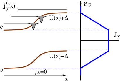
Figure 1: Total dissipationless equilibrium anomalous Hall current flowing in $y$-direction, $J_{y}$, along the potential step $U(x)$ as a function of Fermi energy $\varepsilon_{\rm F}$ for a two-dimensional massive Dirac Hamiltonian with gap $2\Delta$. The labels v,c denote valence- and conduction bands, respectively. The energy distribution of the current density $j^{\varepsilon}_{y}(x)$ is also shown schematically for several values of $\varepsilon$.

We start in Sec. II with the calculation of the total equilibrium current flowing in $y$-direction along a potential step $U(x)$, see Fig. 1. Provided that the potential is constant away from the step, this calculation is exact and valid for any shape of $U(x)$ and any value of the Fermi energy $\varepsilon_{\rm F}$.

Our main findings, summarized in Eq. (17) of section III, concern the total AHE current density in slowly varying electrostatic potentials. For a smooth electrostatic potential $U(\mathbf{r})$, we calculate the current density $\mathbf{j}(\mathbf{r})$ and the energy distribution of the current density $\mathbf{j}^{\varepsilon}(\mathbf{r})$. Electron trajectories with a given energy $\varepsilon$ in two-dimensions cover the areas bounded by the lines of the classical stopping points (having vanishing velocity, $\mathbf{v}=0$). We argue that the energy distribution of the current density $\mathbf{j}^{\varepsilon}(\mathbf{r})$ has the form of a $\delta$-function existing only along these lines of stopping points (cf. Eq. (17)). The ”quantum width” of this $\delta$-function scales like $\Delta r\sim(\hbar^{2}/|\nabla U|)^{1/3}$, being nonperturbative in both Planck’s constant and the electric field.

At the end of the paper, in Sec. IV, we present a semiclassical calculation of the side jump of an electron ray traversing the region with potential step $U(x)$ caused by the AHE, in agreement with Eq. (1). The approach adopted in this section allows us to distinguish and describe within the same calculation both the magnetization part of the current and the pure transport current. Although the content of section IV may appear somewhat methodological, we are not aware of other existing derivations of the anomalous velocity Eq. (1), relying only on the stationary solutions of the Schrödinger(Dirac) equation, without explicit consideration of the time-dependent wave-packet evolution. Interestingly, by considering the stationary ray dynamics (instead of deriving the wave packet equations of motion Eq. (1) MacDonaldRMP10 ; NiuRMP10 ) we were able to find the entire electron’s trajectory in a pedagogically appealing way including the transverse (AHE) shift and show that the magnitude of this shift has an upper bound.

II II. Microscopic calculation of the equilibrium current

We consider the Hamiltonian

$$H=v_{\rm F}(\sigma_{x}p_{x}+\sigma_{y}p_{y})+\Delta\sigma_{z}+U(x)\ .$$ (2)

Here, the Pauli matrices act on the sublattice, valley, or spin degree of freedom depending on the material under consideration. Instead of an uniform electric field, we consider a continuous step-like potential $U(x)$, with $U_{R}=U(x\rightarrow\infty)$ and $U_{L}=U(x\rightarrow-\infty)$. An arbitrarily large electric field $e\mathbf{E}=-\mathbf{\nabla}U$ exists only in a certain region around $x\approx 0$. At large $|x|$, the potential is constant and there is a gap in the spectrum $|\varepsilon-U_{R,L}|<\Delta$, shifted up on the right and down on the left side of the potential step, see Fig. 1. For definiteness, we choose $U_{R}-U_{L}<2\Delta$. We rely here neither on semiclassical nor on weak or constant electric field approximations.

Let $\Psi_{j}(x,y)=e^{ip_{y}y/\hbar}\psi_{j}(x)$ be a complete set of eigenfunctions of the Hamiltonian Eq. (2) with conserved momentum $p_{y_{j}}\equiv p_{y}$. Our goal is to find the transverse current density defined via the velocity operator $\dot{\mathbf{r}}=i[H,\mathbf{r}]/\hbar$ for the Dirac Hamiltonian with $e=-|e|$

$$j_{y}(x)=ev_{\rm F}\langle\sigma_{y}\rangle=ev_{\rm F}\sum_{i,\varepsilon_{i}<\varepsilon_{\rm F}}\psi_{i}^{\dagger}(x)\sigma_{y}\psi_{i}(x)\ .$$ (3)

Our approach to find $j_{y}(x)$ is motivated by the calculation of the out of plane current induced polarization in Rashba wires in Refs. SilvestrovPRL09 ; SilvestrovImryBook10 . Consider the spin-density for a particular stationary state $\psi^{\dagger}(x)\sigma_{x}\psi(x)$,

$$0\equiv\frac{d}{dt}\psi^{\dagger}\sigma_{x}\psi=\frac{i}{\hbar}\psi^{\dagger}[H,\sigma_{x}]\psi{-}v_{\rm F}\partial_{x}(\psi^{\dagger}\psi)\ .$$ (4)

The left and right sides of this equation follow from the calculation of the time derivative in case of the time evolution of the eigenfunction of Eq. (2) taken in two forms $\psi(x,t)=e^{-iHt/\hbar}\psi(x)=e^{-i\varepsilon t/\hbar}\psi(x)$. Then we readily find

$$\Delta\,\psi^{\dagger}\sigma_{y}\psi-v_{\rm F}p_{y}\psi^{\dagger}\sigma_{z}\psi={-}\frac{\hbar v_{\rm F}}{2}\partial_{x}(\psi^{\dagger}\psi)\ .$$ (5)

This relation is enough to find the AHE transverse current for electrons with $p_{y}=0$. The general case with $p_{y}\neq 0$ requires more effort.

Since the conserved momentum $p_{y}$ and $\Delta$ enter the Hamiltonian Eq. (2) in a similar fashion, it is natural to consider a two parameter family of Hamiltonians $H=H(\Delta,p_{y})$. The two eigenfunctions $\psi(\Delta,\pm p_{y})$ of two Hamiltonians $H(\Delta,\pm p_{y})$ (still depending on the coordinate $x$) are related to the eigenfunctions of the same Hamiltonian with $p_{y}=0$ and enlarged mass

$$\psi(\Delta,\pm p_{y})=e^{\pm\frac{i}{2}\theta\sigma_{x}}\psi(\sqrt{\Delta^{2}+v_{\rm F}^{2}p_{y}^{2}},0)\ ,$$ (6)

where $\tan\theta=v_{\rm F}p_{y}/\Delta$. Calculating the expectation values of Eq. (2), we find the following identity relating the expectation values for two solutions with opposite $p_{y}$

$$\Delta\psi^{\dagger}_{+}\sigma_{z}\psi_{+}+v_{\rm F}p_{y}\psi^{\dagger}_{+}\sigma_{y}\psi_{+}$$

$$=\,\, \Delta\psi^{\dagger}_{-}\sigma_{z}\psi_{-}-v_{\rm F}p_{y}\psi^{\dagger}_{-}\sigma_{y}\psi_{-}\ ,$$ (7)

where $\psi_{\pm}=\psi(\Delta,\pm p_{y})$. Here, we used that due to Eq. (6) the values of $\psi^{\dagger}\psi$ and $\psi^{\dagger}\sigma_{x}\partial_{x}\psi$ do not depend on the sign of $p_{y}$.

To find the the equilibrium current where all the states with different sign of $p_{y}$ are occupied equally we only need to know the sum $\psi^{\dagger}_{+}\sigma_{y}\psi_{+}+\psi^{\dagger}_{-}\sigma_{y}\psi_{-}$. Using Eq. (5) to eliminate the terms $\psi_{+}^{\dagger}\sigma_{z}\psi_{+}$ and $\psi_{-}^{\dagger}\sigma_{z}\psi_{-}$ from Eq. (II) we find

$$\psi^{\dagger}_{+}\sigma_{y}\psi_{+}+\psi^{\dagger}_{-}\sigma_{y}\psi_{-}=\frac{-\Delta\hbar v_{\rm F}\,\partial_{x}(\psi^{\dagger}_{+}\psi_{+}+\psi^{\dagger}_{-}\psi_{-})}{2(\Delta^{2}+v_{\rm F}^{2}p_{y}^{2})}.$$ (8)

The r.h.s. here is effectively a derivative of the electron density. Substituting Eq. (8) into Eq. (3) and integrating over $x$ across the potential step leads to the total AHE current

$$J_{y}=J_{R}-J_{L}\ ,\ J_{R(L)}=\frac{-e\Delta\hbar v_{\rm F}^{2}}{2}\sum_{i_{R(L)}}\frac{\psi^{\dagger}_{i_{R(L)}}\psi_{i_{R(L)}}}{\Delta^{2}+v_{\rm F}^{2}p_{y}^{2}}\ .$$ (9)

Since the current density Eq. (3) found with the help of Eq. (8) is an $x$-derivative, the total integrated current may be presented as a difference of two contributions $J_{R}$ and $J_{L}$ depending only on the end-points of integration $x_{R}$ and $x_{L}$. In order to find the universal total current we need to choose these points far to the right and to the left of the step, where the potential is constant.

If the potential $U(x)$ at the points $x_{R}$, $x_{L}$ is flat, one may choose $\psi_{i_{R(L)}}$ in Eq. (9) to be single plane wave solutions of the Dirac equation with either positive or negative $p_{x}$ and calculate the sum over $i$ explicitly. Strictly speaking, any eigenfunction of the Hamiltonian Eq. (2) at least on one side of the potential step $U(x)$ contains both left- ($p_{x}<0$) and right-moving ($p_{x}>0$) waves. Oscillating interference terms between these left- and right-movers which survive the summation in Eq. (9) are the only terms carrying the information about the specific shape of the potential step. These oscillations effectively average out for $x_{R}$, $x_{L}$ taken far away from the step, leading to an exact AHE current, independent of the shape of the potential (cf. Fig. 2 below).

In the case of a slowly varying potential $U(x)$ considered in the next section, Eq. (9) allows us to find the part of the current flowing in a strip $x_{L}<x<x_{R}$ even for points $x_{R(L)}$ inside the step region.

We introduce the valence and conduction band contributions $J_{R(L)}=J_{R(L)}^{c}+J_{R(L)}^{v}$ in Eq. (9). Then

$$J_{R(L)}^{c}=\frac{e}{2h}(U_{R(L)}+\Delta-\varepsilon_{\rm F})\ ,$$ (10)

for $\varepsilon_{\rm F}>\Delta+U_{R(L)}$ and $J_{R(L)}^{c}=0$ otherwise. Integration over the momentum direction in Eq. (9) is done as $\int_{0}^{2\pi}{d\phi}/{(a^{2}+\cos^{2}\phi)}={2\pi}/{a\sqrt{a^{2}+1}}$. The current Eq. (10) is proportional to the difference between the Fermi energy and the conduction band bottom. To find the contribution to the current from the valence band electrons, we perform the summation in Eq. (9) over all occupied states in that band with energies higher than some large negative energy $\varepsilon_{\rm min}$. This gives

$$J_{R(L)}^{v}=\left\{\begin{array}[]{cc}\frac{e}{2h}(\varepsilon_{\rm min}+\Delta-U_{R(L)})\ ,\ \varepsilon_{\rm F}>U_{R(L)}-\Delta\\ \frac{e}{2h}(\varepsilon_{\rm min}-\varepsilon_{\rm F})\ ,\ \varepsilon_{\rm F}<U_{R(L)}-\Delta\end{array}\right..$$ (13)

The dependance on $\varepsilon_{\rm min}$ disappears in the current $J_{y}$ defined in Eq. (9). For electrons with energies smaller than $\varepsilon_{\rm min}$, the density $\psi^{\dagger}\psi$ is constant and the current density, being a derivative of the particle density, Eq. (8) vanishes. With the help of Eqs. (10, 13) we find the total current as a piecewise linear function of $\varepsilon_{\rm F}$ (see Fig. 1)

$$J_{y}=\left\{\begin{array}[]{cc}0\ ,\ \varepsilon_{\rm F}>U_{R}+\Delta\\ \frac{e}{2h}(\varepsilon_{\rm F}-U_{R}-\Delta)\ ,\ U_{R}>\varepsilon_{\rm F}-\Delta>U_{L}\\ \frac{e}{2h}(U_{L}-U_{R})\ ,\ U_{L}+\Delta>\varepsilon_{\rm F}>U_{R}-\Delta\\ \frac{e}{2h}(U_{L}-\Delta-\varepsilon_{\rm F})\ ,\ U_{R}>\varepsilon_{\rm F}+\Delta>U_{L}\\ 0\ ,\ U_{L}-\Delta>\varepsilon_{\rm F}\end{array}\right.,$$ (14)

valid for any shape of the potential step $U(x)$ (we don’t even require monotonous $U(x)$). Generalization of Eq. (14) for $U_{R}-U_{L}>2\Delta$ is presented in the Appendix A. It is not surprising that in the central region in Eq. (14), where $\varepsilon_{\rm F}$ lies in the gap on both sides of the potential step and the system is formally an insulator, there exists a finite constant current. In this paper we consider only the dissipationless equilibrium AHE current, which for $U_{L}+\Delta>\varepsilon_{\rm F}>U_{R}-\Delta$ is carried by the electrons from the fully occupied valence band and does not depend on $\varepsilon_{\rm F}$.

It is interesting to compare the AHE current described by Eq. (14) to the current which would appear in a similar setup with the potential $U(x)$ with an additional quantizing (normal to the $xy$-plane) magnetic field. Due to the drift of electrons‘ Larmor orbits transverse to the electric field each fully occupied Landau level will produce a current in $y$-direction HalperinPRB82 which is twice larger than the AHE current predicted in Eq. (14) in the central region $U_{L}+\Delta>\varepsilon_{\rm F}>U_{R}-\Delta$ (the Fermi energy staying inside the gap at every coordinate $x$). In other words, we may say that electrons from the fully occupied valence band produce an AHE current that is exactly one half of the quantum Hall current due to a single occupied Landau level. For the Fermi energy below the top of the valence band both to the left and to the right of the potential step, $U_{L}-\Delta>\varepsilon_{\rm F}$, the current $J_{y}$ in Eq. (14) disappears which means that only the electrons near the top of this band contribute to the AHE. On the other hand, for the Fermi energy being very high in the conduction band, $\varepsilon_{\rm F}>U_{R}+\Delta$, the AHE disappears again. This means that electrons from the bottom of the conduction band generate an AHE current which is exactly half of the single Landau level current and has the opposite sign compared to the valence band current.

The abrupt disappearance of the total AHE current $J_{y}\equiv 0$, Eq. (14), for energy regions $\varepsilon_{\rm F}>U_{R}+\Delta$ and $\varepsilon_{\rm F}<U_{L}-\Delta$ is rather surprising. A source of the AHE current is attributed to be the Berry anomalous velocity Eq. (1) with $\Omega_{z}(\mathbf{p})=\frac{1}{2}\hbar^{2}\Delta v_{\rm F}^{2}/(\Delta^{2}+p^{2}v_{\rm F}^{2})^{3/2}$ NiuPRL07 . In the case of a monotonous $U(x)$, the last term in Eq. (1) has always the same sign, meaning there is no current cancellation upon summation over electronic states. A vanishing $J_{y}$ in Eq. (14) may become possible only because of contributions to the exact current which are not captured by Eq. (1). Such contributions to the current density, which may be treated semiclassically in the same manner as Eq. (1) are known CooperPRB97 ; XiaoPRL06 . They are named magnetization currents and appear because of an inhomogeneity of electron wave-packet rotation. Even more, we will see in the next section, that the largest contribution to the microscopic current density comes from the reflection regions, where the semiclassical approach is not applicable.

To understand better the spatial distribution of the current Eq. (9) together with the role of interference oscillations between the incoming and outgoing waves, neglected in Eqs. (10-14), we describe below a numerically exact current density in a constant electric field.

III III. Current density in a smooth potential

We choose the potential in Eq. (2) to be $U(x)=Fx-\Delta$. In this paper we consider Dirac Hamiltonians with a gap large enough to neglect tunneling between the bands. The large insulating gap means that in order to investigate the AHE current along the border of an electron Fermi liquid it is enough to take only the conduction band electrons with energies slightly above the gap into account, i.e. the non-relativistic limit $|p_{y}v_{\rm F}|,|Fx|\ll\Delta$ with the spinor wave-function (See Appendix B.)

$$\psi^{T}=e^{ip_{y}y}(\phi(x),0)\ ,\ \phi(x)={\rm Ai}((x-x_{c})/x_{0})\ .$$ (15)

Here, $\rm Ai(x)$ is the Airy function, $x_{0}=(\hbar^{2}v_{\rm F}^{2}/(\Delta F))^{1/3}$ and $x_{c}=\varepsilon/F-p_{y}^{2}v_{\rm F}^{2}/(2\Delta F)$ and the energy of an electron in the conduction band is $|\varepsilon|\ll\Delta$.

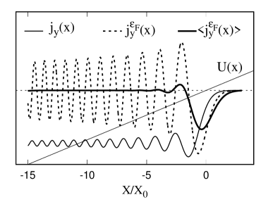
Figure 2: Anomalous Hall current density (conduction band, $e=-|e|$) for $U(x)=Fx-\Delta$ and $\varepsilon_{\rm F}=0$. Distances are measured in units of $x_{0}=(\hbar^{2}v_{\rm F}^{2}/(\Delta F))^{1/3}$. The vertical axis has arbitrary units. The thin solid line is the current density $j_{y}(x)$. The step-like current density is formed at distances $\sim x_{0}$ from the edge. The dashed line shows the energy distribution of the current density $j_{y}^{\varepsilon_{\rm F}}(x)$ and the thick solid line is $\langle j_{y}^{\varepsilon_{\rm F}}(x)\rangle$ smoothed with the function $\exp(-(x-x^{\prime})^{2}/x_{0}^{2})$. The clear $\delta$-function character of $\langle j_{y}^{\varepsilon_{\rm F}}(x)\rangle$ shows that $j_{y}^{\varepsilon_{\rm F}}(x)$ will also behave effectively like a $\delta$-function when folded with an arbitrary function varying slowly on the scale $\sim x_{0}$.

As we already mentioned, we will from now on consider only the case of potentials with a relatively small slope, $Fx_{0}\ll\Delta$. For steeper potentials, with $Fx_{0}\sim\Delta$, Eq. (15) will be no longer valid and one needs to consider the tunneling of relativistic electrons between the conduction and valence bands. However, the electrons from the conduction band and from the valence band generate AHE currents of opposite signs. So the total AHE is likely to be diminished in the case of tunneling. This may be seen also from Appendix A, where we consider the extension of Eq. (14) (which is valid for arbitrary strong electric fields $dU/dx$, but where the tunneling is forbidden energetically) for the case of a large potential step, $U_{R}-U_{L}>2\Delta$, where tunneling is possible.

The current due to a single state Eq. (15) is considered in Appendix B. In Fig. 2, we show the total density of the conduction band current, $j_{y}(x)$, for $\varepsilon_{\rm F}=0$ obtained after summation over the energy and $p_{y}$-momentum. The details of the calculation are given also in Appendix B. Besides the interference oscillations, the figure agrees well with the step function form

$$j_{y}(x)=\frac{e}{2h}F\,\theta(-x)\ .$$ (16)

We stress that this result for small $F$ may be derived directly from Eq. (9). The current flowing in $y$-direction to the left of point $x$ is given by Eqs. (9, 10) with $U_{R}$ replaced by $U(x)$. Differentiating with respect to $x$ gives Eq. (16). This derivation shows that Eq. (16) is also valid at large distances, $|Fx|\gtrsim\Delta$.

The authors of Ref. LenskyPRL15 considered the AHE for Dirac electrons in an electric field, but taking into account only the transport current caused by the Berry velocity Eq. (1). For $|Fx|\ll\Delta$ their result, $j_{y}(x)=(e/2h)(xF^{2}/\Delta)\,\theta(-x)$, is parametrically smaller than Eq. (16). It is, however, unclear, how one can exclusively observe the equilibrium transport current. Further discussions of the comparison with Ref. LenskyPRL15 are given in Appendix B.

Features of the semiclassical intrinsic AHE for massive Dirac Hamiltonians are best revealed by the energy distribution of the current density $\mathbf{j}^{\varepsilon}(\mathbf{r})$, also considered in Ref. CooperPRB97 and defined as $\mathbf{j}(\mathbf{r})=\int^{\varepsilon_{\rm F}}\mathbf{j}^{\varepsilon}(\mathbf{r})d\varepsilon$. Numerical plots in Fig. 2 show that $\mathbf{j}^{\varepsilon}(\mathbf{r})$ in a uniform electric field is mathematically equivalent to the $\delta$-function in the $\hbar\rightarrow 0$ limit. This means that we may expect that $\mathbf{j}^{\varepsilon}(\mathbf{r})$ will be concentrated along the lines $U(\mathbf{r})=\varepsilon-\Delta$ in the case of an arbitrary slowly varying two-dimensional potential also. Thus, we can write

$$\mathbf{j}^{\varepsilon}(\mathbf{r})=\frac{e}{2h}\,\,\delta(\varepsilon-U(\mathbf{r})-\Delta)\,\,\mathbf{n}_{z}\times\mathbf{\nabla}U(\mathbf{r})\ .$$ (17)

This formula is the central result of our paper. The exact shape of the $\delta$-function may be deduced from Eqs. (45, 46) of Appendix B

$$\delta(\varepsilon-U(\mathbf{r})-\Delta)|\mathbf{\nabla}U|\rightarrow\frac{d}{dr_{\perp}}\int_{0}^{\infty}{\rm Ai}^{2}(\xi^{2}+\frac{r_{\perp}}{r_{0}})d\xi\ ,$$ (18)

where $r_{\perp}=(\varepsilon-U(\mathbf{r})-\Delta)/|\mathbf{\nabla}U|$ is the distance between $\mathbf{r}$ and the equipotential line $U(\mathbf{r})=\varepsilon-\Delta$ and ${\rm Ai}$ is again the Airy function. The width of the $\delta$-function, nonperturbative both in $\hbar$ and in the electric field, is $r_{0}=(\hbar^{2}v_{\rm F}^{2}/(\Delta|\mathbf{\nabla}U(\mathbf{r})|))^{1/3}$.

The shape of the $\delta$-function Eq. (18) is illustrated in Fig. 2. At first glance, the curve shown in the figure does not seem a good approximation for the $\delta$-function due to its large oscillations. Nevertheless, the period of these oscillations decreases fast with increasing $r_{\perp}$  (or $x$ in the figure) and in the limit $r_{0}\rightarrow 0$ ($x_{0}\rightarrow 0$) it satisfies the property of the functional $\int\delta(x)f(x)dx=f(0)$ for any smooth $f(x)$.

Equation (17) is valid if $|\partial^{2}U/\partial{r_{i}}^{2}|\,r_{0}\ll|\mathbf{\nabla}U|$. Absence of inter-band tunneling requires $r_{0}|\mathbf{\nabla}U|\ll\Delta$. A simple direct proof of Eq. (17) in the nonrelativistic limit is given in Appendix C.

The $\delta$-function Eq. (17) is peaked at the border of the area accessible classically at the energy $\varepsilon$. This defines the line of stopping points, where both components of the momentum of an electron reaching such a point vanish. Inside this area $\mathbf{j}^{\varepsilon}(\mathbf{r})=0$. (see also Fig. 5 and the discussion in Appendix B.)

For the valence band Eq. (17) changes sign. The total current density $j^{c}_{y}(x)+j^{v}_{y}(x)$ vanishes everywhere where the Fermi energy stays locally inside the conduction or the valence band. For example, in the case of a sufficiently strong and smooth disorder potential the Fermi energy may cross several times both the bottom of the conduction and the top of the valence bands. The sample in this case, even being insulating on average, will consist of large electron and hole puddles separated by the big insulating regions. Our theory in this case predicts the vanishing AHE current inside the puddles and existence of the AHE in the insulating parts between the puddles.

IV IV. Ray dynamics and magnetization currents

The eigenfunction of the Hamiltonian Eq. (2) in the semiclassical limit may be written in the form (we use $\hbar=v_{\rm F}=1$ in this section)

$$\psi(x)=\sqrt{1/v_{x}}\,e^{i\int^{x}p(x^{\prime})dx^{\prime}}[1+\beta(x)\sigma_{y}]\phi\ .$$ (19)

Here, $\phi^{T}(x)=\frac{1}{\sqrt{2}}\left(\sqrt{1+\xi},\sqrt{1-\xi}\right)$, $\xi=\Delta/\sqrt{\Delta^{2}+p^{2}}$ and $p(x)=\sqrt{(\varepsilon-U(x))^{2}-\Delta^{2}}$. For illustrative purposes we only consider the case of an incident ray parallel to the potential gradient. The classical longitudinal velocity of electrons in the ray is $v_{x}=p/\sqrt{\Delta^{2}+p^{2}}=p/(\varepsilon-U)$. (Arbitrary incident angles may be considered with the help of Eq. (6))

The coefficient $\beta$ in Eq. (19), responsible for the expectation value of the anomalous velocity, may be found by acting with $\psi(x)$ on the Hamiltonian Eq. (2), as is shown in Appendix D. Alternatively, the value of $\beta$ may be extracted in the linear approximation in $U^{\prime}=dU/dx$ from the exact Eq. (8) in which we substitute the wave function Eq. (19). Doing so, we find

$$\langle v_{y}\rangle=\frac{\psi^{\dagger}\sigma_{y}\psi}{\psi^{\dagger}\psi}=2\beta=\frac{-U^{\prime}\Delta}{2p^{2}\sqrt{\Delta^{2}+p(x)^{2}}}\ .$$ (20)

This velocity is bigger, and even much bigger if $p(x)\ll\Delta$, than the AHE velocity deduced from Eq. (1). However, Eq. (20) does not provide the true information about the transverse transport, since the solution $\psi(x)$ extends indefinitely along the $y$-axis. Even more, as we show below, the term $\sim\beta$ in the wave function Eq. (19) simply does not contribute to the electrons’ trajectory.

To find the actual bending of the trajectory, we need to consider a ray of electrons

$$\Psi(x,y)=\int f(p_{y})\psi_{p_{y}}(x,y)dp_{y}\ ,$$ (21)

where $\psi_{p_{y}}(x,y)$ are the solutions of the Dirac equation Eq. (2) with finite momentum $p_{y}$ along the potential step, having all the same energy $\varepsilon$ and the narrow function $f(p_{y})$ is peaked at $p_{y}=0$.

For small $p_{y}$, Eq. (6) gives $\psi_{p_{y}}(x,y)=e^{ip_{y}y}(1+i\sigma_{x}{p_{y}}/{(2\Delta)})\psi(x)$ and Eq. (21) becomes

$$\Psi=\left(1+\frac{\sigma_{x}}{2\Delta}\frac{\partial}{\partial y}\right)g(y)\psi(x)\ ,$$ (22)

where $g(y)=\int dke^{iky}f(k)$ is a smooth envelope function in $y$ direction of a ray propagating mostly along the $x$-axis. It is convenient to choose $g(y)$ almost flat within some region $\delta y\gg 1/p(x)$ which smoothly goes to zero outside the region, see Fig. 3.

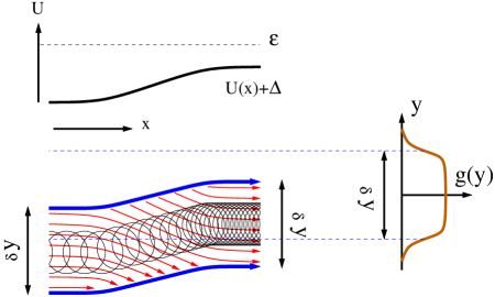
Figure 3: The electron ray with width $\delta y$ traversing the region of a smooth potential step $U(x)$ with energy $\varepsilon>\Delta+U$. Blue lines are the borders of the ray with approximately constant electron density inside (envelope function $g(y)$). Red lines show the velocity field $\langle\mathbf{v}\rangle=\langle\mathbf{\sigma}\rangle$. There is a side jump of the ray during crossing the electric field area, $dU/dx\neq 0$, consistent with the anomalous velocity $\mathbf{v}_{B}=\mathbf{\Omega}\times\mathbf{\nabla}U/\hbar$, Eq. (1). According to Eqs. (23, 24) the ray is always shifted downwards. The magnitude of the shift is bigger for larger velocity $v_{x}$, or, equivalently, for larger $\varepsilon-U(x)$. Circles inside the ray show how the nonuniform electron’s magnetization results in a current. The density of the circles (magnetization), rotating counter-clockwise, increases to the right on the figure.

To find explicitly the transverse displacement of the ray we rewrite Eq. (22) as

$$\Psi=g\left(y+\frac{1}{2\Delta}\right)\psi_{+}(x)+g\left(y-\frac{1}{2\Delta}\right)\psi_{-}(x)\ ,$$ (23)

where we use the decomposition of $\psi(x)$ into the $\sigma_{x}$ eigenvectors, $\psi=\psi_{+}+\psi_{-}$ and $\sigma_{x}\psi=\psi_{+}-\psi_{-}$. The trajectory $y(x)$ is now found as (see Fig. 3)

$$y(x)=\frac{1}{2\Delta}\frac{-\psi^{\dagger}(x)\sigma_{x}\psi(x)}{\psi^{\dagger}(x)\psi(x)}=\frac{-p(x)}{2\Delta\sqrt{\Delta^{2}+p(x)^{2}}}\ .$$ (24)

The shift of the trajectory $y(x)$ exists already for the wave function Eq. (19) in zeroth order in $U^{\prime}$ when the term $\sim\beta$ is omitted. The transverse transport velocity is now

$$v_{y{\rm tr}}=v_{x}\frac{dy}{dx}=\frac{U^{\prime}\Delta}{2(\Delta^{2}+p(x)^{2})^{3/2}}\ ,$$ (25)

in accordance with Eq. (1).

Both the distribution of the local velocity $\langle\mathbf{v}\rangle$ (with the $y$-component $\langle\mathbf{v}_{y}\rangle$ given by Eq. (20)) and the shift of the ray $y(x)$ Eq. (24) are shown in Fig. 3. It is hard to show in the figure what happens in the narrow region at the borders of the ray, where the red lines of the velocity field cross the ray border shown in blue. An accurate description of the charge balance at such borders is presented in Appendix E, where it gives yet another way to find the anomalous velocity Eq. (20) and the coefficient $\beta$, see Eq. (79).

The total current is the sum of the transport part ($\mathbf{j}_{tr}$) and a magnetization contribution ($\mathbf{\nabla}\times\mathbf{M}(\mathbf{r})$ with $\mathbf{M}(\mathbf{r})$ being the magnetic moment density) CooperPRB97 ,

$$\mathbf{j}=\mathbf{j}_{tr}+\mathbf{\nabla}\times\mathbf{M}(\mathbf{r})\ .$$ (26)

In Appendix E we use $M(\mathbf{r})$ available in the literature NiuPRL07 to show that our results Eqs. (20, 25) indeed agree with Eq. (26). For an electron in the valence band $\mathbf{M}(\mathbf{r})$ is larger in the regions with higher potential $U(x)$. Consequently, in Fig. 3, we illustrate the magnetization current $\mathbf{\nabla}\times\mathbf{M}(\mathbf{r})$, Eq. (26), by drawing circles with a coordinate dependent density.

The transport (Eq. (25)) and the total (Eq. (20)) anomalous Hall currents in Fig. 3 flow in opposite directions. However, the figure shows the semiclassical current Eq. (20) due to a single injected electron ray. In the case of the equilibrium AHE there will be many such rays, including the ones reflected by the potential. The total equilibrium transverse current – flowing in the direction suggested by Eq. (1) – originates from the narrow reflection regions, Eq. (17), not captured by Eqs. (19, 20). This shows again the importance of our results that go beyond the semiclassical treatment.

Considering an electron ray instead of a wave packet MacDonaldRMP10 ; NiuRMP10 allows us at once to find the entire trajectory Eq. (24). Interestingly, the anomalous shift of the trajectory Eqs. (23, 24) turned out to have an exact upper bound, $|y|<1/(2\Delta)$.

V V. Conclusions

In this paper, we calculated the total local AHE current for electrons described by the massive Dirac Hamiltonian. The exact results turned out to be strongly universal in the case where the potential $U(x)$ depends only on one coordinate. What is even more surprising, the current which we found for an arbitrarily smooth potential $U(\mathbf{r})$ turns out to be much stronger (and its energy/coordinate dependance much sharper) than the usually considered Berry curvature-induced currents. For example, the equilibrium anomalous Hall currents exist if the Fermi energy lies inside the insulating gap, but disappear abruptly if $\varepsilon_{\rm F}$ is shifted into the conduction or valence band. The width of the transition is governed by the weakness of the electric field or the size of the sample. It will be interesting to see this sharp Fermi energy dependance in measurements of the quantum Kerr and Faraday effects for the surface states in three-dimensional topological insulators FaradayExp .

Another promising direction for further research lies in the understanding of the relations between the non-dissipative equilibrium bulk AHE currents considered here and the protected edge currents found in the topological insulators inpreparation

Acknowledgements.– Discussions with Sunghun Park, P. W. Brouwer, C. W. J. Beenakker, I. V. Gornyi and C. De Beule are greatly acknowledged. This work was supported by the DFG grant RE 2978/8-1.

VI Appendix A: Anomalous Hall current for the case $U_{R}-U_{L}>2\Delta$

Here, we consider the generalization of the formula Eq. (14) to the case of a large potential step $U(x)$ with a magnitude that exceeds the value of the gap in the electron spectrum, $U_{R}-U_{L}>2\Delta$.

As in the main text, we assume that far away from the step the potential $U(x)$ became flat with the asymptotic values $U_{R},U_{L}$. That means we may still perform explicitly a summation over all occupied states in Eq. (9) to obtain the same Eqs. (10, 13). Integration over the momentum direction in Eq. (9) is done as $\int_{0}^{2\pi}{d\phi}/{(a^{2}+\cos^{2}\phi)}={2\pi}/{a\sqrt{a^{2}+1}}$. Rewritten in a more detailed form, Eqs. (10, 13) become (note that the electron’s charge is negative, $e=-|e|$)

$$J_{R}^{c}=\left\{\begin{array}[]{cc}\frac{e}{2h}(U_{R}+\Delta-\varepsilon_{\rm F})\ ,\ \varepsilon_{\rm F}>U_{R}+\Delta\\ 0\ ,\ \varepsilon_{\rm F}<U_{R}+\Delta\end{array}\right.,$$ (29)

$$J_{L}^{c}=\left\{\begin{array}[]{cc}\frac{e}{2h}(U_{L}+\Delta-\varepsilon_{\rm F})\ ,\ \varepsilon_{\rm F}>U_{L}+\Delta\\ 0\ ,\ \varepsilon_{\rm F}<U_{L}+\Delta\end{array}\right.,$$ (32)

and

$$J_{R}^{v}=\left\{\begin{array}[]{cc}\frac{e}{2h}(\varepsilon_{\rm min}+\Delta-U_{R})\ ,\ \varepsilon_{\rm F}>U_{R}-\Delta\\ \frac{e}{2h}(\varepsilon_{\rm min}-\varepsilon_{\rm F})\ ,\ \varepsilon_{\rm F}<U_{R}-\Delta\end{array}\right.,$$ (35)

$$J_{L}^{v}=\left\{\begin{array}[]{cc}\frac{e}{2h}(\varepsilon_{\rm min}+\Delta-U_{L})\ ,\ \varepsilon_{\rm F}>U_{L}-\Delta\\ \frac{e}{2h}(\varepsilon_{\rm min}-\varepsilon_{\rm F})\ ,\ \varepsilon_{\rm F}<U_{L}-\Delta\end{array}\right..$$ (38)

As we explained in the main text, $\varepsilon_{\rm min}$ is the lower bound of the integral(sum) over energies in Eq. (9) which cancels out from the current $J_{y}$. Electrons with energies below $\varepsilon_{\rm min}$ do not contribute to the current since for them the derivative of the density $\partial_{x}\psi^{\dagger}\psi$ vanishes in Eq. (8). We assume that there is no contribution to AHE from the bottom (ultraviolet cutoff) of the valence band. The formal proof of the latter will be given elsewhere inpreparation .

The band structure in the presence of a large potential step is shown in Fig. 4 and needs to be compared to Fig. 1. The five regimes of different current behaviors $J_{y}(\varepsilon_{\rm F})$ in Fig. 1 represent (from lower to higher energies $\varepsilon_{\rm F}$) metallic, half-metallic, insulating, half-metallic and metallic phases. Here, metallic refers to $\varepsilon_{\rm F}$ lying inside the conduction or valence band, insulating means that $\varepsilon_{\rm F}$ always lies inside the gap and half-metallic means that $\varepsilon_{\rm F}$ is inside the gap only on one side (half plane) of the potential step. The sequence of regimes in Fig. 4 is metallic, half-metallic, metal-metal, half-metallic and metallic where the metal-metal regime corresponds to two half-plane metals separated by a tunnel barrier. The total anomalous Hall current for the setup in Fig. 4 found from Eqs. (9, 29, 35) is

$$J_{y}=\left\{\begin{array}[]{cc}0\ ,\ \varepsilon_{\rm F}>U_{R}+\Delta\\ \frac{e}{2h}(\varepsilon_{\rm F}-U_{R}-\Delta)\ ,\ U_{R}+\Delta>\varepsilon_{\rm F}>U_{R}-\Delta\\ -\frac{e}{h}\Delta\ ,\ U_{R}-\Delta>\varepsilon_{\rm F}>U_{L}+\Delta\\ \frac{e}{2h}(U_{L}-\Delta-\varepsilon_{\rm F})\ ,\ U_{L}+\Delta>\varepsilon_{\rm F}>U_{L}-\Delta\\ 0\ ,\ U_{L}-\Delta>\varepsilon_{\rm F}\end{array}\right.,$$ (39)

valid again for any shape of the potential step $U(x)$. The main difference to Eq. (14) is the smaller current in the central metal-metal regime, i.e. $J_{y}=-\frac{e}{h}\Delta$ instead of $J_{y}=\frac{e}{h}(U_{L}-U_{R})$.

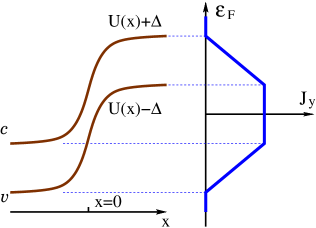
Figure 4: Similar to Fig. 1, but for $U_{R}-U_{L}>2\Delta$: total anomalous Hall current $J_{y}$ flowing along the potential step $U(x)$ as a function of the Fermi energy $\varepsilon_{\rm F}$ for the two-dimensional massive Dirac Hamiltonian with a spectral gap $2\Delta$.

VII Appendix B: current density in an uniform electric field

Like in the main text, we consider here a linear potential $U(x)=Fx-\Delta$ and assume the nonrelativistic limit of the conduction band electrons, i.e. $|Fx|\ll\Delta$, $|p_{y}v_{\rm F}|\ll\Delta$. The Dirac equation Eq. (2) for the spinor wave function $\psi^{T}=(\phi,\chi)$ reduces in this case to an non-relativistic Schrödinger equation for the upper component, $\phi$, with the lower component being negligibly small, $|\chi|\ll|\phi|$,

$$\left(\frac{p^{2}}{2m}+Fx\right)\phi=\varepsilon\phi\ ,\ \chi=\frac{p_{x}+ip_{y}}{2mv_{\rm F}}\phi\ .$$ (40)

Here, the mass $m$ is related to the gap parameter via $\Delta=mv_{\rm F}^{2}$. The Schrödinger equation for $\phi$ is solved by the Airy function as used in Eq. (15) of the main text. In this limit, the anomalous Hall current density Eqs. (9, 10) becomes proportional to the derivative of the electron charge density

$$j_{y}(x)=-e\frac{\hbar}{2m}\partial_{x}\rho(x)\ .$$ (41)

Also without the loss of generality we may put Fermi energy equal to zero, $\varepsilon_{\rm F}=0$.

VII.1 Current for a single electron

We start by considering the current density Eq. (41) contributed by a single electronic state described by the wave function Eq. (15). The result of such a calculation, shown in Fig. 5 for $p_{y}=\varepsilon=0$, demonstrates strong interference oscillations between incoming and reflected electron waves. As follows from the asymptotic form of the Airy function for large negative $x$, the oscillation amplitude stays constant but its period decreases like $\sim 1/|x|^{3/2}$.

In order to visualize the semiclassical part of the current density we smooth out the interference oscillations by averaging the density at each point $x$ with the weight functions $e^{-((x-x^{\prime})/x_{0})^{2}}$ and $e^{-((x-x^{\prime})/x_{0})^{2}/2}$ in Fig. 5. Assuming an oscillation amplitude of unity, the semiclassical current density at large negative $x$ is small like $1/(4|x|^{3/2})$. Therefore, we have to enlarge the smoothed current density in the figure in order to make the semiclassical current density visible.

The smoothed current density shown in Fig. 5 (thick solid line) has two distinct features. The first was already mentioned. It is the positive power law tail of $j_{y}(x)$ for large negative values of $x$. (Only at this tail the current density may be explained by Eq. (20) for the special case of a weak linear potential.) The second is the large negative ($e=-|e|$) bump of the current density at the reflection point $x=0$. The current density, Eq. (41), is proportional to the derivative of the electron density, which in the semiclassical limit is $\rho(x)\sim 1/\sqrt{-x}$ at large negative $x$ and $\rho(x)\approx 0$ at positive $x$. That is why both the power law tail of $j_{y}(x)$ and the negative bump are inevitable and survive the smoothing procedure. The total single-electron current integrated over $x$ vanishes in the non-relativistic approximation Eq. (15). The negative bump of the current density at the reflection point is responsible for the vanishing of the current density energy distribution $\mathbf{j}^{\varepsilon}(\mathbf{r})$ inside the classically accessible area, see Eq. (17). (Note that $\mathbf{j}^{\varepsilon}(\mathbf{r})$ is a sum of currents due to many electrons with the same energy $\varepsilon$, while Fig. 5 shows only the single electron current.)

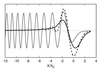
Figure 5: Anomalous Hall current density $j_{y}(x)$ for a single electron (conduction band) with energy $\varepsilon=0$ and $p_{y}=0$ for the linear potential $U(x)=Fx-\Delta$. Distances are measured in units of $x_{0}=(\hbar^{2}v_{\rm F}^{2}/(\Delta F))^{1/3}$. The thin solid line shows the current density Eq. (41) with strong oscillations having constant amplitude at negative $x$. To reveal the smooth semiclassical contribution to the current density we show the plot of the same current smoothed with weights $\exp(-((x-x^{\prime})/x_{0})^{2})$ (dashed line) and $\exp(-((x-x^{\prime})/x_{0})^{2}/2)$ (thick solid line). We do not specify the units at the vertical axis, but the relative amplitude for the smoothed curves is multiplied by a factor of $4$.

VII.2 Summing up the current contributions due to many electrons

The semiclassical electron density in the conduction band is given by the integral

$$\rho=\int_{\varepsilon<\varepsilon_{\rm F}}\frac{d^{2}p}{(2\pi\hbar)^{2}}=\frac{2}{(2\pi\hbar)^{2}}\int\frac{d\varepsilon_{x}dp_{y}}{d\varepsilon_{x}/dp_{x}}\ ,$$ (42)

where $\varepsilon_{x}=p_{x}^{2}/(2m)$ and the coordinate-dependance emerges through the limits of integration, $\varepsilon=\mathbf{p}^{2}/2m+Fx<\varepsilon_{\rm F}$. To make a connection between this formula and the wave function Eq. (15) we notice that the smooth part of the squared Airy function, representing the semiclassical density, using the negative $x$ asymptotics may be written as (here $p_{y}=0$, generalization for finite $p_{y}$ is obvious, see Eq. (44) below)

$$\langle{\rm Ai}^{2}\left(\frac{x}{x_{0}}\right)\rangle=\frac{\sqrt{x_{0}}}{2\pi\sqrt{-x}}=\frac{\sqrt{2mFx_{0}}}{2\pi p_{x}(x)}=\frac{\sqrt{2Fx_{0}/m}}{2\pi d\varepsilon_{x}/dp_{x}}\ ,$$ (43)

where we have used $p_{x}(x)=\sqrt{-2mFx}$ and $\langle...\rangle$ denotes the average procedure. Consequently, we may replace the semiclassical density of the conduction band electrons Eq. (42) by the exact formula

$$\rho(x)=\frac{1}{\pi\hbar^{2}\sqrt{2Fx_{0}/m}}$$ (44)

$$\times \int_{\varepsilon_{x}>0}{\rm Ai}^{2}\left(\frac{\varepsilon_{x}+p_{y}^{2}/2m+Fx}{Fx_{0}}\right)d\varepsilon_{x}dp_{y}\ .$$

The absence of electrons with energies above the Fermi energy, $\varepsilon_{\rm F}=0$, is taken care of automatically due to the exponential suppression of the Airy function for positive arguments, so there is no need to introduce an upper limit of integration over either $\varepsilon_{x}$ or $|p_{y}|$.

With the help of Eq. (41) we may find the current density

$$j_{y}(x)=\frac{eF}{2\pi m\hbar\sqrt{2Fx_{0}/m}}$$ (45)

$$\times \int_{\varepsilon_{y}>0}{\rm Ai}^{2}\left(\frac{\varepsilon_{y}+Fx}{Fx_{0}}\right)dp_{y}\ .$$

This formula is used for calculating the current density in Fig. 2. The easiest way to find the energy distribution of the current density $j^{\varepsilon}_{y}(x)$ is by differentiating Eq. (45) to obtain

$$j_{y}^{\varepsilon=0}(x)=\frac{1}{F}\frac{\partial}{\partial x}j_{y}(x)\ .$$ (46)

This result is shown in Fig. 2.

Replacing the squared Airy function by its asymptotic behavior we find the semiclassical density of the anomalous Hall current (valid only for negative $x$)

$$j_{y}(x)=\frac{eF}{4\pi^{2}\hbar}\int_{0}^{-Fx}\frac{d\varepsilon_{y}}{\sqrt{\varepsilon_{y}(|Fx|-\varepsilon_{y})}}\ .$$ (47)

Upon energy integration we arrive at Eq. (16), $j_{y}(x)\propto\theta(-x)$.

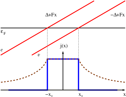
Figure 6: Top - Energy bands structure. Bottom - Comparison of the density of the anomalous Hall current found in this paper (solid-blue) with the current density due to side jumps only LenskyPRL15 (dashed-brown) around the band crossing by the Fermi energy in a strong electric field.

VII.3 Comparison to existing results

Our results for the anomalous Hall current density for the massive Dirac Hamiltonian (e.g. Eq. (16) of the main text) differ substantially from the calculation of dissipationless bulk currents in a recent paper Ref. LenskyPRL15 where only the transport contribution to the anomalous Hall current caused by the Berry velocity in Eq. (1) was taken into account. For the potential $U=Fx$ (shifted by $\Delta$ from what we used before) and the Fermi energy $\varepsilon_{\rm F}=0$ the authors of Ref. LenskyPRL15 have found the total (conduction plus valence band) density of anomalous current in the form

$$j_{y}(x)=\left\{\begin{array}[]{cc}j_{0}&,\ |x|<x_{0}\\ j_{0}x_{0}/|x|&,\ |x|>x_{0}\end{array}\right.\ \ ,\ \ j_{0}=\frac{|e|F}{2h}\ .$$ (48)

Here $x_{0}=\Delta/F$ and $x=\pm x_{0}$ are the classical turning points for the conduction and valence band electrons at the Fermi energy. (Note that the total current $\int j_{y}(x)dx$ diverges logarithmically.)

Our approach for a sufficiently small $F$ would give instead of Eq. (48) the current density

$$j_{y}(x)=\left\{\begin{array}[]{cc}j_{0}&,\ |x|<x_{0}\\ 0&,\ |x|>x_{0}\end{array}\right.\ \ ,\ \ j_{0}=\frac{|e|F}{2h}\ .$$ (49)

The current density is constant and proportional to the electric field only when the Fermi energy lies in the gap between two bands.

The results Eq. (48) and Eq. (49) are compared in Fig. 6. As we mentioned already, the reason for the difference between Eqs. (48) and (49) is that the authors of Ref. LenskyPRL15 calculate only the transport current caused by the Berry velocity contribution Eq. (1) to the motion of the center of the wave packet. Our derivation, starting from the calculation of the expectation value of the velocity operator automatically includes both the motion of its center and the inhomogeneous rotation of the wave-packet, creating the magnetization current. Although it was argued CooperPRB97 ; XiaoPRL06 that the magnetization current is irrelevant for transport phenomena, it is necessary for finding e.g. the magnetic moment of the electron gas.

Taking into account only the conduction band contribution to the current near the Fermi energy crossing with the bottom of the conduction band in Eq. (49) gives

$$j_{y}(x)=\frac{e}{2h}F\,\theta(-x_{0}-x)\ ,$$ (50)

which is the same as Eq. (16) with shifted coordinate due to a different definition of the constant electric field potential. Analogously, extracting the conduction band current from Eq. (48) at $x\approx-x_{0}$ gives (for the Fermi energy above the top of the valence band and only slightly above the bottom of the conduction band, valence band electrons give a large constant contribution to the current, while the linear in $x$ (at $|x-x_{0}|\ll x_{0}$) part of $j_{y}(x)$ comes from the conduction band electrons)

$$j_{y}(x)=\frac{-e}{2h}\frac{(x_{0}+x)F^{2}}{\Delta}\theta(-x_{0}-x)\ ,$$ (51)

which is parametrically smaller than our result. The linear increase of the current in Eq. (51) reflects the fact that the electron density in a two-dimensional non-relativistic electron gas in a constant electric field increases linearly with the coordinate. All these electrons have the same anomalous velocity Eq. (1). The current density of Eq. (50) is much more singular than Eq. (51) and leads to the $\delta$-function energy distribution of the current density $\mathbf{j}^{\varepsilon}(\mathbf{r})$, Eq. (17).

VII.4 Vanishing of $\mathbf{j}^{\varepsilon}(\mathbf{r})$

Integration over energy in Eq. (47) gives a step-shaped current density Eq. (16). Differentiating this result like in Eq. (46) gives a $\delta$-function energy distribution of the current density $j_{y}^{\varepsilon}(x)$. Vanishing of $j_{y}^{\varepsilon}(x)$ almost everywhere except the close vicinity of the line $\Delta+U(x)-\varepsilon=0$ allows us to suggest a general $\delta$-function formula for the current in arbitrary smooth potential $U(\mathbf{r})$, Eq. (17).

The $\delta$-function Eq. (17) peaks at the border of the area accessible classically at the energy $\varepsilon$. This is the line of stopping points where both components of momentum of an electron reaching the point vanish. Inside this area $\mathbf{j}^{\varepsilon}(\mathbf{r})=0$, which is somewhat surprising since the semiclassical current density (given by the $\sim 1/|x|^{3/2}$ tail of the smoothed density in Fig. 5) for each electron is always of the same sign. The only current of the ”wrong” sign, ensuring the vanishing of the current density distribution, is the negative bump in the smoothed current density in Fig. 5 at the classical turning point. Through every point $\mathbf{r}$ there exist two trajectories with energy $\varepsilon$ and momentum $\mathbf{p}$ normal to the local electric field. These are trajectories having a turning point in the sense of Fig. 5 and the ”negative bump” in the current density at $\mathbf{r}$.

VIII Appendix C: Explicit proof of the formula for $\mathbf{j}^{\varepsilon}(\mathbf{r})$.

In this Appendix we first give a proof of Eq. (17) in the nonrelativistic limit by calculating the current carried by the conduction band electrons for a smooth two-dimensional potential and a Fermi energy only slightly above the insulating gap.

Consider the Dirac Hamiltonian

$$H=v_{\rm F}(\sigma_{x}p_{x}+\sigma_{y}p_{y})+\Delta\sigma_{z}+U(\mathbf{r})-\Delta\ .$$ (52)

Calculation of the anomalous Hall current (carried e.g. by the conduction band electrons) becomes especially easy when $|U(\mathbf{r})|\ll\Delta$.

Let the eigenfunction of $H$ in Eq. (52) have the form

$$\psi=\left(\begin{array}[]{cc}\phi\\ \chi\end{array}\right)\ .$$ (53)

Substituting this into Eq. (52) in the limit $|\varepsilon|\ll\Delta$, $|U|\ll\Delta$, one readily recovers the nonrelativistic Schrödinger equation

$$\left(\frac{p^{2}}{2m}+U(\mathbf{r})\right)\phi=\varepsilon\phi\ ,\ \chi=\frac{-i\hbar\partial_{x}+\hbar\partial_{y}}{2mv_{\rm F}}\phi\ .$$ (54)

Here, $\Delta=mv_{\rm F}^{2}$. We refer to the electron state described by the Dirac Hamiltonian Eq. (52) with at least one component of momentum effectively comparable to $\Delta/v_{\rm F}$ as relativistic and the electron described by the Eq. (54) as nonrelativistic. The two components of the current $\mathbf{j}=ev_{\rm F}\langle\mathbf{\sigma}\rangle$ are now found as (compare to Eq. (8))

$$\psi^{\dagger}\sigma_{y}\psi=-\frac{\hbar v_{\rm F}}{2\Delta}\partial_{x}\phi^{*}\phi -\frac{i\hbar v_{\rm F}}{2\Delta}[\phi^{*}\partial_{y}\phi-(\partial_{y}\phi^{*})\phi]\ ,$$

$$\psi^{\dagger}\sigma_{x}\psi=\frac{\hbar v_{\rm F}}{2\Delta}\partial_{y}\phi^{*}\phi -\frac{i\hbar v_{\rm F}}{2\Delta}[\phi^{*}\partial_{x}\phi-(\partial_{x}\phi^{*})\phi]\ .$$ (55)

Here, the second terms on the r.h.s. of both equations have the form of the usual currents in non-relativistic quantum mechanics, whereas anomalous Hall current is given by the first terms. The electron density in the semiclassical and non-relativistic approximation is

$$\sum_{\varepsilon_{i}<\varepsilon_{\rm F}}\psi_{i}^{\dagger}\psi_{i}=\int_{\frac{p^{2}}{2m}+U<\varepsilon_{\rm F}}\frac{d^{2}p}{(2\pi\hbar)^{2}}=\theta(\varepsilon_{\rm F}-U)\frac{m(\varepsilon_{\rm F}-U)}{4\pi\hbar^{2}}\ .$$ (56)

Combining Eqs. (VIII) and (56) we obtain

$$\mathbf{j}(\mathbf{r})=\frac{e}{2h}\,\,\theta(\varepsilon_{\rm F}-U(\mathbf{r}))\,\,\mathbf{n}_{z}\times\mathbf{\nabla}U(\mathbf{r})\ ,$$ (57)

where $\mathbf{n}_{z}$ is the unit vector normal to the $(x,y)$ plane. Differentiating this with respect to $\varepsilon_{\rm F}$ gives $\mathbf{j}^{\varepsilon_{\rm F}}(\mathbf{r})$ of Eq. (17).

Our derivation of Eq. (57) for a smooth two-dimensional potential $U(\mathbf{r})$ relies on the nonrelativistic approximation Eq. (54). The energy distribution of the current density $\mathbf{j}^{\varepsilon}(\mathbf{r})$ found from Eq. (57) vanishes everywhere except in the narrow region around the line of stopping points $\varepsilon-U(\mathbf{r})=0$. But the electron in a smooth potential near a stopping point is always nonrelativistic. This suggests that the range of validity of the result Eq. (57) may be larger than just the nonrelativistic limit $|U(\mathbf{r})|\ll\Delta$, but it may be valid for an arbitrarily large (and still smooth) two-dimensional potential $U(\mathbf{r})$.

Indeed, Eqs. (14, 16) of the main text (second of those is the exact analog of Eq. (57)) were found for an arbitrarily large smooth potential but only depending on one coordinate $U(\mathbf{r})\equiv U(x)$. That means, all what is left to do in order to prove Eqs. (57,17) for an arbitrarily large Fermi energy is to show that the contribution to the anomalous current from the electrons with high energy has the form of a local expansion in powers of the gradients of the potential. In other words, the anomalous current at a point $\mathbf{r}$ caused by the electrons with $\varepsilon-U(\mathbf{r})\gtrsim\Delta$ must be a function of the gradient, $\mathbf{\nabla}U(\mathbf{r})$, found at the same point.

To find the current density for an arbitrarily strong two-dimensional potential one may take the wave function Eq. (19) and sum up the currents due to all occupied states. However, we may simply notice that the anomalous velocity Eq. (20) due to the solution Eq. (19) depends only on the local derivative of the potential $U^{\prime}$. This means that if Eqs. (17, 57) are valid for arbitrary $\varepsilon_{\rm F}$ in an arbitrarily strong uniform electric field, they should be also valid for an arbitrarily smooth potential $U(\mathbf{r})$ for a large Fermi energy $\varepsilon_{\rm F}\sim\Delta$.

IX Appendix D: Calculation of $\beta(x)$.

In this Appendix, we calculate explicitly starting from the semiclassical solution of Eq. (2) the coefficient $\beta(x)$ entering the wave function Eq. (19) of the main text. This coefficient is responsible for the emergence of a finite expectation value of the anomalous velocity $\langle v_{y}\rangle$ in Eq. (20). In the main text we avoid the direct calculation of $\beta(x)$ and use instead Eq. (8) to calculate $\langle v_{y}\rangle$. Similar to the corresponding part of the main text, we use here $\hbar=v_{\rm F}=1$.

Let the conduction band electron described by the massive Dirac Hamiltonian Eq. (2) have an energy $\varepsilon$ well above the smooth potential $U(x)$ and a vanishing (conserved) $y$-momentum, $p_{y}=0$. We may then introduce a coordinate-dependent classical momentum in $x$-direction

$$p_{x}=p(x)=\sqrt{(\varepsilon-U(x))^{2}-\Delta^{2}}\ .$$ (58)

The single plane wave solution may now be presented in the form (in the case of reflection, which we do not consider here, there will be a superposition of two such counter-propagating solutions)

$$\psi=e^{i\int^{x}p(x^{\prime})dx^{\prime}}[a(x)\phi_{+}+b(x)\phi_{-}]\ ,$$ (59)

where

$$\phi_{+}=\frac{1}{\sqrt{2\sqrt{p^{2}+\Delta^{2}}}}\left(\begin{array}[]{cc}\sqrt{\sqrt{p^{2}+\Delta^{2}}+\Delta}\\ \sqrt{\sqrt{p^{2}+\Delta^{2}}-\Delta}\end{array}\right)\ ,$$ (62)

$$\phi_{-}=\frac{1}{\sqrt{2\sqrt{p^{2}+\Delta^{2}}}}\left(\begin{array}[]{cc}\sqrt{\sqrt{p^{2}+\Delta^{2}}-\Delta}\\ -\sqrt{\sqrt{p^{2}+\Delta^{2}}+\Delta}\end{array}\right),$$ (65)

are the positive and negative energy eigenvectors in the limit of a flat $U(x)$.

The wave function Eq. (59) is in principle exact, provided one can find the coefficients $a(x)$ and $b(x)$ to all orders in the small $U^{\prime},U^{\prime\prime},\cdots$. Substituting Eq. (59) into the Dirac equation leads to an (exact) system of linear equations

$$-ia^{\prime}+i\frac{U^{\prime}\Delta}{2p\sqrt{\Delta^{2}+p^{2}}}b+2\Delta b=0\ ,$$ (66)

$$-ib^{\prime}-i\frac{U^{\prime}\Delta}{2p\sqrt{\Delta^{2}+p^{2}}}a+2p\,b=0\ .$$

Approximate solutions of the system of equations (66) (which we are interested in) may be found iteratively. First, in the second equation, we may neglect a small derivative $b^{\prime}$ compared to $2pb$, leading to

$$b\approx i\frac{U^{\prime}\Delta}{4p^{2}\sqrt{\Delta^{2}+p^{2}}}\,a\ .$$ (67)

Substituting this into the first equation of Eq. (66) and neglecting the small second order term $\sim U^{\prime}b$ we find

$$a\approx\sqrt{\frac{\sqrt{\Delta^{2}+p^{2}}}{p}}\ .$$ (68)

The fact that this solution reproduces correctly the classical electron density

$$\rho\approx|a|^{2}\sim 1/v_{x}\ ,$$ (69)

is an additional crosscheck.

Eq. (19) of the main text is reproduced after we notice that

$$\beta=ib/a\ .$$ (70)

X Appendix E: Magnetization current vs. transport AHE current.

In this Appendix, we consider in more details the division of the total anomalous Hall current into the transport and magnetization currents discussed in the last part of the main paper. Like in the main text, we put $\hbar=v_{\rm F}=1$. Also like in the main text we are going to consider the transverse shift and transverse current distribution in a wide electron ray injected parallel to the $x$-axis and parallel to the electric field ($U(\mathbf{r})\equiv U(x)$) described by the wave function Eq. (21). Ray injection with an arbitrary incident angle may be considered with the help of Eq. (6) of the main text. It is constructive to consider the envelope function $g(y)$ (Eq. (22)) to be flat, $g(y)\approx 1$, over the large region $\delta y$ (i.e. $p_{x}\,\delta y\gg 1$) with also very smooth steps towards $g=0$ outside this region, cf. Fig. 3.

By calculating the longitudinal current $j_{x}=e\Psi^{\dagger}\sigma_{x}\Psi$ and the density $\rho=e\Psi^{\dagger}\Psi$ from Eq. (23) we find

$$j_{x}=eg^{2}\left(y+\frac{1}{2\Delta}\right)\psi_{+}^{\dagger}\psi_{+}-eg^{2}\left(y-\frac{1}{2\Delta}\right)\psi_{-}^{\dagger}\psi_{-}\ ,$$

$$\rho=eg^{2}\left(y+\frac{1}{2\Delta}\right)\psi_{+}^{\dagger}\psi_{+}+eg^{2}\left(y-\frac{1}{2\Delta}\right)\psi_{-}^{\dagger}\psi_{-}\ .$$ (71)

We remind that $\Psi=\Psi(x,y)$ is the wave function of a ray propagating mostly in $x$-direction, Eq. (21), and $\psi=\psi(x)$ is the plane-wave solution Eq. (19) with momentum parallel to the electric field ($p_{y}\equiv 0$). The components of $\psi(x)$ in the $\sigma_{x}$ eigenvalue basis are $\psi_{+}=\frac{1}{2}(1+\sigma_{x})\psi$ and $\psi_{-}=\frac{1}{2}(1-\sigma_{x})\psi$. The second equation (X) was used in the main text to calculate the side-jump of the trajectory Eq. (24).

Now we may use the fact that for our choice of the normalization of the wave function Eq. (19) $\psi_{+}^{\dagger}\psi_{+}-\psi^{\dagger}_{-}\psi_{-}=1$ and $\psi_{+}^{\dagger}\psi_{+}+\psi^{\dagger}_{-}\psi_{-}=1/v_{x}$ and write instead of Eq. (X)

$$j_{x} =eg^{2}\left(y\right)+eg^{\prime}g/(\Delta v_{x})\ ,$$

$$\rho =eg^{2}\left(y\right)/v_{x}+eg^{\prime}g/\Delta\ ,$$ (72)

where $v_{x}=v_{x}(x)$ acquires a dependance on $x$ in the case of a smooth potential $U(x)$,

$$v_{x}=\frac{p(x)}{\sqrt{\Delta^{2}+p(x)^{2}}}\ ,\ p(x)=\sqrt{(\varepsilon-U(x))^{2}-\Delta^{2}}\ .$$ (73)

The second equality in Eq. (X) may be rewritten as

$$\rho=eg^{2}(y+v_{x}/(2\Delta))/v_{x}\ ,$$ (74)

which immediately gives the trajectory (equivalent to Eq. (24) of the main text)

$$y(x)=-\frac{v_{x}(x)}{2\Delta}\ .$$ (75)

Differentiating this $y(x)$ allowed us in the main text to find the transverse velocity $v_{y{\rm tr}}$ Eq. (25). Since this velocity originates from the displacement of the ray and not from the wave-packet’s internal dynamics, it leads to the transport anomalous current $j_{y{\rm tr}}=v_{y{\rm tr}}\rho$.

The possible time evolution of the quantum ray Eq. (21) should proceed in agreement with the continuity equation. Since the ray is built from waves of the same energy, the charge distribution is stationary and the continuity equation reduces to the vanishing of the divergence of the current, ${\rm div}\,\mathbf{j}=0$. Thus we write

$$\frac{\partial j_{x}}{\partial x}=-e\frac{g^{\prime}gv_{x}^{\prime}}{\Delta v_{x}^{2}}=-\frac{\partial j_{y}}{\partial y}\ ,$$ (76)

where $g^{\prime}=dg/dy$ and $v_{x}^{\prime}=dv_{x}/dx$. The current $j_{y}$ here can not be derived directly from the wave function Eq. (22). It appears due to the correction $\sim\beta\sigma_{y}$ to the semiclassical wave-function in Eq. (19), which was omitted in Eq. (22) (and consequently in Eqs. (X)). Still the continuity equation Eq. (76) allows us to find this current. The total anomalous current density $j_{y}$ is expected to be independent of the transverse coordinate $y$ only inside the ray, where $g(y)\approx 1$. At the borders of the ray $j_{y}$ increases from zero (outside) to this constant value. This increase is described by Eq. (76). Integration over $y$ of the second equality in Eq. (76) gives the value of the anomalous current inside the ray

$$j_{y}=e\frac{g^{2}v_{x}^{\prime}}{2\Delta v_{x}^{2}}\ .$$ (77)

The calculation of the derivative of the longitudinal velocity $v_{x}^{\prime}$ here gives

$$v_{x}^{\prime}=\frac{dv_{x}}{dp}\frac{dp}{dx} =\frac{\Delta^{2}}{(\Delta^{2}+p^{2})^{3/2}}\times\frac{-U^{\prime}}{p}\sqrt{\Delta^{2}+p^{2}}$$

$$=\frac{-U^{\prime}\Delta^{2}}{p(\Delta^{2}+p^{2})}\ ,$$ (78)

leading to

$$j_{y} =-eg^{2}U^{\prime}\frac{\Delta}{2p^{3}}\ ,$$ (79)

$$\langle v_{y}\rangle =\frac{j_{y}}{\rho}=\frac{-U^{\prime}\Delta}{2p^{2}\sqrt{\Delta^{2}+p^{2}}}\ ,$$

in agreement with Eq. (20) of the main text. Thus we see that the anomalous transverse current inside the ray (and the velocity Eq. (20)), which is not captured by Eqs. (21, 22, 23) follows from them through the continuity equation. Eq. (79) shows the total microscopic AHE current for which the corresponding velocity $\langle v_{y}\rangle$ can not be deduced from Eq. (1).

As was written in the main text, the difference between the total microscopic and transport current densities is naturally attributed to the magnetization current CooperPRB97

$$\mathbf{j}=\mathbf{j}_{tr}+\mathbf{j}_{mag}\ ,\ \mathbf{j}_{mag}=\mathbf{\nabla}\times\mathbf{M}(\mathbf{r})\ ,$$ (80)

with $\mathbf{M}(\mathbf{r})$ being the density of the magnetic moment. According to Ref. NiuPRL07 the magnetic moment of an electron subject to the massive two-dimensional Dirac Hamiltonian is

$$\mu(p)=\frac{e}{2\hbar}\frac{mv_{\rm F}^{2}}{m^{2}v_{\rm F}^{2}+p^{2}}=\frac{e\Delta}{2(\Delta^{2}+p^{2})}\ .$$ (81)

That gives the magnetization density

$$M=\mu\Psi^{\dagger}\Psi=\mu/v_{x}=\frac{e\Delta}{2p\sqrt{\Delta^{2}+p^{2}}}\ .$$ (82)

Consequently, we find, in agreement with the general expectation CooperPRB97 ; XiaoPRL06 ,

$$-\frac{\partial M}{\partial x}=-\frac{eU^{\prime}\Delta}{2}\left(\frac{1}{p^{3}}+\frac{1}{p(\Delta^{2}+p^{2})}\right)=j_{y}-j_{y_{tr}}\ .$$ (83)

With that we have explicitly demonstrated that the spatially inhomogeneous magnetization is responsible for the difference between the total current and the transport current.

References

- (1) C.L. Kane and E.J. Mele, Phys. Rev. Lett. 95, 226801 (2005). Quantum Spin Hall Effect in Graphene.
- (2) B.A. Bernevig, T.L. Hughes, and S.C. Zhang, Science 314, 1757 (2006). Quantum Spin Hall Effect and Topological Phase Transition in HgTe Quantum Wells.
- (3) R. V. Gorbachev, J. C. W. Song, G. L. Yu, A. V. Kretinin, F. Withers, Y. Cao, A. Mishchenko, I. V. Grigorieva, K. S. Novoselov, L. S. Levitov, A. K. Geim, Science 346, 448 (2014). Detecting topological currents in graphene superlattices.
- (4) K. F. Mak, K. L. McGill, J. Park, and P. L. McEuen, Science 344, 1489 (2014). The valley Hall effect in transistors.
- (5) Y. Shimazaki, M. Yamamoto, I. V. Borzenets, K. Watanabe, T. Taniguchi and S. Tarucha, Nat. Phys. 11, 1032,(2015). Generation and detection of pure valley current by electrically induced Berry curvature in bilayer graphene.
- (6) N. Nagaosa, J. Sinova, S. Onoda, A. H. MacDonald, and N. P. Ong, Rev. Mod. Phys. 82, 1539 (2010). Anomalous Hall effect.
- (7) D. Xiao, M.-C. Meng, and Q. Niu, Rev. Mod. Phys. bf 82, 1959 (2010). Berry phase effects on electronic properties.
- (8) M.-C. Chang and Q. Niu, Phys. Rev. B 53, 7010 (1996). Berry phase, hyperorbits, and the Hofstadter spectrum: Semiclassical dynamics in magnetic Bloch bands.
- (9) G. Sundaram and Q. Niu, Phys. Rev. B 59, 14915 (1999). Wave-packet dynamics in slowly perturbed crystals: Gradient corrections and Berry-phase effects.
- (10) N. R. Cooper, B. I. Halperin, and I. M. Ruzin, Phys. Rev. B 55, 2344 (1997). Thermoelectric response of an interacting two-dimensional electron gas in a quantizing magnetic field.
- (11) D. Xiao, Y. Yao, Z. Fang, and Q. Niu, Phys. Rev. Lett. 97, 026603 (2006). Berry-Phase Effect in Anomalous Thermoelectric Transport.
- (12) V. A. Volkov and S. A. Mikhailov, JETP Lett. 41, 476 (1985). Quantization of the Faraday effect in systems with a quantum Hall effect.
- (13) K.N. Okada, Y. Takahashi, M. Mogi, R. Yoshimi, A. Tsukazaki, K.S. Takahashi, N. Ogawa, M. Kawasaki, and Y. Tokura, Nat. Commun. 7, 12245 (2017). Terahertz spectroscopy on Faraday and Kerr rotations in a quantum anomalous Hall state. L.Wu, M. Salehi, N. Koirala, J. Moon, S. Oh, and N.P. Armitage, Science 354, 1124 (2016). Quantized Faraday and Kerr rotation and axion electrodynamics of a 3D topological insulator. V. Dziom, A. Shuvaev, A. Pimenov, G. V. Astakhov, C. Ames, K. Bendias, J. Böttcher, G. Tkachov, E. M. Hankiewicz, C. Brüne, H Buhmann, L. W. Molenkamp, Nat. Commun. 8, 15197 (2017). Observation of the universal magnetoelectric effect in a 3D topological insulator.
- (14) X.-L. Qi, T.L. Hughes, and S.-C. Zhang, Phys. Rev. B 78, 195424 (2008). Topological field theory of time-reversal invariant insulators.
- (15) D. Xiao, W. Yao, and Q. Niu, Valley-Contrasting Physics in Graphene: Magnetic Moment and Topological Transport, Phys. Rev. Lett. 99, 236809 (2007).
- (16) D. Xiao, G.-B. Liu, W. Feng, X. Xu, and W. Yao , Coupled Spin and Valley Physics in Monolayers of and Other Group-VI Dichalcogenides, Phys. Rev. Lett. 108, 196802 (2012)
- (17) Y. D. Lensky, J. C. W. Song, P. Samutpraphoot, L. S. Levitov, Phys. Rev. Lett. 114, 256601 (2015). Topological Valley Currents in Gapped Dirac Materials.
- (18) P. G. Silvestrov, V. A. Zyuzin, and E. G. Mishchenko, Phys. Rev. Lett. 102, 196802 (2009). Mesoscopic Spin-Hall Effect in 2D electron systems with smooth boundaries.
- (19) P. G. Silvestrov and E. G. Mishchenko, Spin-Hall Effect in Chiral Electron Systems: from Semiconductor Heterostructures to Topological Insulators, ”Perspectives of Mesoscopic Physics” - Dedicated to Yoseph Imry’s 70th Birthday, World Scientific, 2010.
- (20) B. I. Halperin, Phys. Rev. B 25, 2185 (1982). Quantized Hall conductance, current-carrying edge states, and the existence of extended states in a two-dimensional disordered potential.
- (21) P.G. Silvestrov and P. Recher, in preparation.