Stochastic modified equations for the asynchronous stochastic gradient descent

Abstract

We propose stochastic modified equations (SMEs) for modeling the asynchronous stochastic gradient descent (ASGD) algorithms. The resulting SME of Langevin type extracts more information about the ASGD dynamics and elucidates the relationship between different types of stochastic gradient algorithms. We show the convergence of ASGD to the SME in the continuous time limit, as well as the SME’s precise prediction to the trajectories of ASGD with various forcing terms. As an application, we propose an optimal mini-batching strategy for ASGD via solving the optimal control problem of the associated SME.

1 Introduction

In this paper, we consider the following empirical risk minimization problem commonly encountered in machine learning:

$$\min_{x\in\mathbb{R}^{d}}f(x):=\frac{1}{n}\sum_{i=1}^{n}f_{i}(x),$$ (1.1)

where $x$ represents the model parameters, $f_{i}(x)\equiv f(x;z_{i})$ denotes the loss function of the training sample $z_{i}$, and $n$ is the size of the training sample set. Since the training set for most applications is of large size, stochastic gradient descent (SGD) is the most popular algorithm used in practice. In the simplest scenario, SGD samples one random instance $f_{i}(\cdot)$ uniformly at each iteration and updates the parameter by evaluating only the gradient of the selected $f_{i}(\cdot)$. The stability and convergence rate of SGD have been studied in depth, for example, see [9, 17]. However, the scalability of SGD is unfortunately restricted by its inherent sequential nature. To overcome this issue and hence accelerate the convergence, there has been a line of research devoted to asynchronous parallel SGDs. In the distributed computation scenario, an asynchronous stochastic gradient descent (ASGD) method parallelizes the computation on multiple processing units by (1) calculating multiple gradients simultaneously at different processors and (2) sending the results asynchronously back to the master for updating the model parameters [1, 21].

1.1 Related Work

There has been a vast literature on the analysis of SGD, see for example Bottou et al. [3] for a comprehensive review of this subject. Some widely-used methods include AdaGrad [5], which extends SGD by adapting step sizes for different features, RMSProp [24], which resolves AdaGrad’s rapidly diminishing learning rates issue, and Adam [11], which combines the advantages of both AdaGrad and RMSProp with a parameter learning rates adaption based on the average of the second moments of the gradients. On the other hand, relatively few studies are devoted to ASGDs. Most of these studies for ASGD take an optimization perspective. Hogwild! [21] assumed data sparsity in order to run parallel SGD without locking successfully. Under various smoothness conditions on $f$ such as $f$ being strongly convex and $f_{i}$’s all Lipschitz, it showed that the convergence rate can be similar to the synchronous case. Duchi et al. [6] extended this result by developing an asynchronous dual averaging algorithm that allows problems to be non-smooth and non strongly-convex as well. Mitliagkas et al. [16] observed that a standard queuing model of asynchrony correlates to the momentum, that is, asynchrony produces momentum in SGD updates. There are also several methods using asynchrony either in parallel or in a distributed way, such as asynchronous stochastic coordinate descent algorithms [14, 15, 18, 22].

Recently, Li et al. [13] introduced the concept of the stochastic modified equation for SGDs (referred as SME-SGD in this report), where in the continuous-time limit an SGD is approximated by an appropriate (overdamped) Langevin equation. Compared to most convergence analyses that give upper bounds for (strongly) convex objects, this new framework not only provides more precise analyses for the leading order dynamics of SGD but also suggests adaptive hyper-parameter strategies using optimal control theory.

1.2 Our Contributions

We give a novel derivation of SMEs for the ASGD algorithms by introducing auxiliary variables to treat an effective memory term. With the derived SME models, we are able to characterize the dynamics of ASGD algorithms.

In Section 2, we first derive a stochastic modified equation for the asynchronous stochastic gradient descent, denoted shortly as SME-ASGD, for the case where each loss function $f_{i}$ is quadratic. The derivation results in a Langevin equation, which by assuming its ergodicity has a unique invariant distribution solution with a convergence rate dominated by the temperature factor. Meanwhile, for the momentum SGD (MSGD), a similar Langevin equation denoted as SME-MSGD is derived and we show that the temperature factors for both derived SME agree. This comparison gives a Langevin dynamics explanation of why an asynchronous method gives rise to similar behavior as compared to the momentum-based methods [16]. Then by introducing a new accumulative quantity, we derive a more general SME-ASGD for the general case in which the gradient of the loss function can be nonlinear. We show that the two SME-ASGDs are equivalent when the objective functions are quadratic. We remark that the presented results make use of a few simplifying approximations which are made in a non-rigorous and non-quantified manner, e.g, assuming the noise coefficients to be constant $\sigma$ and the accumulation of i.i.d noise.

Section 3 provides some numerical analysis for SME-ASGD by providing a strong approximation estimation to the ASGD algorithm. Different from the usual convergence studies, we do not assume convexity on $f$ or $f_{i}$ but only require their gradients to be (uniformly) Lipschitz. Numerical results including non-linear forcing terms and non-convex objectives demonstrate that SME-ASGD provides much more accurate predictions for the behavior of ASGD compared to SME-SGD derived in [13]. In Section 4, we apply the optimal control theory to identify the optimal mini-batch for ASGD and the numerical simulations there verify that the suggested strategy gives a significantly better performance.

2 Stochastic Modified Equations

The asynchronous stochastic gradient descent (ASGD) carries out the following update at each step:

$$x_{k+1}=x_{k}-\eta\nabla f_{\gamma_{k}}(x_{k-\tau_{k}}),$$ (2.1)

where $\eta$ is the step size, $\{\gamma_{k}\}$ are i.i.d. uniform random variables taking values in $\{1,2,\cdots,n\}$, and $x_{k-\tau_{k}}$ is the delayed read of the parameter $x$ used to update $x_{k+1}$ with a random staleness $\tau_{k}$.

Assumption 1.

We assume that the staleness $\tau_{k}$ are independent and that the sample selection process $\gamma_{k}$ is mutually independent from the staleness process $\tau_{k}$. $\nabla f_{i}$’s are all (uniformly) Lipschitz, that is, for each $1\leq i\leq n$, there exists $L_{i}>0$ such that for any $x,y\in\mathbb{R}^{d}$, we have $|\nabla f_{i}(x)-\nabla f_{i}(y)|\leq L_{i}|x-y|$. As a consequence, by taking $L=\frac{1}{n}\sum_{i=1}^{n}L_{i}$, $\nabla f$ is also (uniformly) Lipschitz: $|\nabla f(x)-\nabla f(y)|\leq L|x-y|$. In addition, the staleness process $\tau_{k}$ follows the geometric distribution: $\tau_{k}=l$ (i.e., $x_{k-\tau_{k}}=x_{k-l}$), $l\in\{0,1,2,\cdots\}$, with probability $(1-\mu)\mu^{l}$ for $\mu\in(0,1)$.

Assumption 2.

We assume that the equations SME-ASGD (2.5) and SME-MSGD (2.1) are ergodic.

The geometric distribution assumption here is not only made to simplify the computation, but also can be justified by considering the canonical queuing model [25]. For example, the computation at each processor may involve a randomized algorithm that requires each processor to do multiple independent trials until the result is accepted, thus resulting in a geometrically distributed computation time. The geometric staleness assumption has been used in the previous asynchrony analysis, for example, see [16]. Our derivation of SME models can be also easily generalized to other random staleness models if the memory kernel, i.e., the distribution of staleness in time, decays sufficiently fast for integrability and is completely monotone when we approximate the memory kernel by a $C^{\infty}(0,\infty)$ function $\kappa(r)$. $\kappa(r)$ is completely monotone if for all for $n\geq 0,~{}r>0,~{}(-1)^{n}\frac{d^{n}}{dr^{n}}\kappa(r)\geq 0.$ Under that circumstance, we can approximate the kernel accurately by $\sum_{k=1}^{n_{k}}c_{k}e^{-\lambda_{k}r}$ using the Bernstein’s theorem of monotone functions [2], and each term can be embedded into one auxiliary value to derive the SME formulation.

2.1 Linear gradients

We first show the derivation of Langevin dynamics with the linear forcing term. Suppose that, for each $1\leq i\leq n,\nabla f_{i}$ is linear, or equivalently each $f_{i}$ is quadratic. While this is a fairly restrictive assumption, the derivation in this simplified scenario offers a more transparent view towards the stochastic modified equation for the asynchronous algorithm.

A key quantity for our derivation is the expected read $m_{k}$ defined as the expectation of $x_{k}$ following Assumption 1:

$$m_{k}=\mathbb{E}_{\tau}(x_{k-\tau_{k}})=\sum\nolimits_{l=0}^{\infty}x_{k-l}(1-\mu)\mu^{l}.$$

Here $m_{k}$ is a conditional expectation conditioned on the history of $x$, and $m_{k}$ is random since $x_{k-l}$’s are. Note that $m_{k+1}=\sum_{l=0}^{\infty}x_{k+1-l}(1-\mu)\mu^{l}=x_{k+1}(1-\mu)+\mu m_{k}$ and $x_{k+1}=(m_{k+1}-\mu m_{k})/(1-\mu)$. Plugging this into (2.1), we can rewrite ASGD as

$$\frac{m_{k+1}-2m_{k}+m_{k-1}}{\eta(1-\mu)}=-\frac{m_{k}-m_{k-1}}{\eta}-\nabla f(m_{k})+(\nabla f(m_{k})-\nabla f_{\gamma_{k}}(x_{k-\tau_{k}})).$$ (2.2)

The left hand side and the first term on the right hand side of (2.2) can be viewed as divided difference approximations to various time derivatives of $m$. The second term on the right hand side is the usual gradient. The last term $\nabla f(m_{k})-\nabla f_{\gamma_{k}}(x_{k-\tau_{k}})$ can be understood as the noise due to stochastic gradient and the read delays; it has mean $0$, since the expectation, conditioned on the history of updates, can be decomposed as

$$\mathbb{E}_{\gamma,\tau}\bigl{(}\nabla f(m_{k})-\nabla f_{\gamma_{k}}(m_{k})+\nabla f_{\gamma_{k}}(m_{k})-\nabla f_{\gamma_{k}}(x_{k-\tau_{k}})\bigr{)}=\frac{1}{n}\sum_{i=1}^{n}(\nabla f(m_{k})-\nabla f_{i}(m_{k}))\\ +\frac{1}{n}\sum_{i=1}^{n}\big{(}\nabla f_{i}(\sum_{l=0}^{\infty}x_{k-l}(1-\mu)\mu^{l})-\sum_{m=0}^{\infty}(1-\mu)\mu^{m}\nabla f_{i}(x_{k-m})\big{)}=0.$$

The covariance matrix of the noise will be denoted as

$$\Sigma_{k}=\mathbb{E}_{\gamma,\tau}\bigl{(}(\nabla f(m_{k})-\nabla f_{\gamma_{k}}(x_{k-\tau_{k}}))(\nabla f(m_{k})-\nabla f_{\gamma_{k}}(x_{k-\tau_{k}}))^{T}\bigr{)},$$

conditioned on $\{x_{k-l}\}_{l\geq 0}$ and we also denote the square root of $\Sigma_{k}$ by $\sigma_{k}$, i.e., $\Sigma_{k}=\sigma_{k}\sigma_{k}^{T}$. $\Sigma_{k}$ (and thus $\sigma_{k}$) in general depends on the previous history of the trajectory, although such dependence is omitted in our notation.

In order to arrive at a continuous time stochastic modified equation from (2.2), we view $m_{k}$ as the evaluation of a function $m$ at time points $t_{k}=k\Delta t$ where $\Delta t$ is the effective time step size for the corresponding stochastic modified equation, and it is chosen as $\Delta t=\sqrt{\eta(1-\mu)}$. By introducing the auxiliary variable $p_{k}=\frac{1}{\Delta t}(m_{k}-m_{k-1})$, we can reformulate (2.2) as a system of $(m_{k},p_{k})$:

$$p_{k+1} =p_{k}-\Delta t\sqrt{(1-\mu)/\eta}p_{k}-\Delta t\nabla f(m_{k})+\Delta t\,\bigl{(}\nabla f(m_{k})-\nabla f_{\gamma_{k}}(x_{k-\tau_{k}})\bigr{)},$$ (2.3)

$$m_{k+1} =m_{k}+\Delta t\,p_{k+1}.$$ (2.4)

To obtain an SME, we first model the random term by a Gaussian random noise, that is, $\Delta t\bigl{(}\nabla f(m_{k})-\nabla f_{\gamma_{k}}(x_{k-\tau_{k}})\bigr{)}\sim\sigma_{k}(\eta(1-\mu))^{1/4}\Delta B_{t}$, where $\Delta B_{t}=B_{t+\Delta t}-B_{t}$ is the increment of a Brownian motion (thus $\mathbb{E}(\Delta B_{t})=0$ and $\mathbb{E}(\Delta B_{t}\Delta B_{t}^{T})=\Delta t$) and the coefficient is chosen to match the variance. Such modelling is valid because the random variables $\gamma_{k}$ and $\tau_{k}$ are independent to each other, and the choices are independent at each iteration, we can approximate the i.i.d random random term by Gaussian noise in the weak sense. Assuming that $\Delta t$ is small, we arrive at a Langevin type equation:

$$dP_{t} =-\nabla f(M_{t})dt-\sqrt{(1-\mu)/\eta}P_{t}dt+\sigma(t)(\eta(1-\mu))^{1/4}dB_{t},$$ (2.5)

$$dM_{t} =P_{t}dt,$$

where $\Sigma(t)=\Sigma(\{M_{s}\}_{0\leq s<t},\{P_{s}\}_{0\leq s<t})$ has the evolution equation (the derivation is deferred to Appendix A)

$$d\Sigma_{t}= -\sqrt{\frac{1-\mu}{\eta}}\Sigma_{t}dt-\mu(\nabla f(M_{t})\nabla f(P_{t})^{T}+\nabla f(P_{t})\nabla f(M_{t})^{T})dt-\sqrt{\frac{1-\mu}{\eta}}\nabla f(M_{t})\nabla f(M_{t})^{T}dt$$

$$+\mu\sqrt{\eta(1-\mu)}\nabla f(P_{t})\nabla f(P_{t})^{T}dt+\frac{1}{n}\sqrt{\frac{1-\mu}{\eta}}\sum_{i=1}^{n}\nabla f_{i}(M_{t}+\mu\sqrt{\frac{\eta}{1-\mu}}P_{t})\nabla f_{i}(M_{t}+\mu\sqrt{\frac{\eta}{1-\mu}}P_{t})^{T}dt.$$

When $f$ is a smooth confining potential, that is, $f$ satisfies $\lim_{|x|\to+\infty}f(x)=+\infty$ and $e^{-\beta f(x)}\in L^{1}(\mathbb{R}^{d})$ for all $\beta\in\mathbb{R}^{+}$ (an example for $f$ is being a quadratic potential), the process approaches to the minimum of the potential function, and $\sigma(t)$ (as the damping term $-\sqrt{(1-\mu)/\eta}\Sigma_{t}dt$ dominates in the evolution equation) can be approximated by a constant matrix $\sigma$ up to a first order approximation for large time $t$. When this constant matrix $\sigma$ is a multiple of the identity matrix, say $\sigma=\varsigma I$, $(P_{t},M_{t})$ in the standardized model is an ergodic Markov process with stationary distribution [19]:

$$\rho_{\infty}(p,m)=Z^{-1}e^{-\beta(\frac{1}{2}|p|^{2}+f(m))},$$

where $Z$ is a normalization constant. In this case, the resulting friction is $\sqrt{(1-\mu)/\eta}$ and the temperature $\beta^{-1}$ is $\frac{1}{2}\varsigma^{2}\eta$. When the constant matrix $\sigma$ is not a multiple of identity (but still being constant), the stationary distribution takes a similar form in a transformed coordinate system. We remark that though in theory proving time-inhomogeneous process (2.5) has a unique stationary distribution is beyond the scope of this paper, the numerical observations suggest that such a constant approximation of the noise coefficient does not change the process’ property fundamentally; in the numerical experiments, we observe that the trajectory of SME-ASGD does not change much when we replace the coefficient of noise by a constant matrix.

The reason why we care about the temperature parameter here is that it quantifies the variance of the noise and therefore gives us more information about the asymptotic behavior of the optimization process. With such a tool, we can better analyze the connection between different stochastic gradient algorithms. Let us illustrate it by showing one example here: Mitliagkas et al. [16] argues that there is some equivalence between adding asynchrony or momentum to the SGD algorithms, and they showed it by taking expectation to a simple queuing model and finding matched coefficients. Here, we investigate such relation by looking at the corresponding Langevin dynamics, specifically the temperature for both SMEs, thus offering a more detailed dynamical comparison.

Stochastic gradient descent with momentum (MSGD) introduced by [20] utilizes the velocity vector from the past updates to accelerate the gradient descent [23]:

$$v_{k+1}=\mu^{\prime}\,v_{k}-\eta^{\prime}\nabla f_{\gamma_{k}}(x_{k}),$$ (2.6)

$$x_{k+1}=x_{k}+v_{k+1},$$

with a momentum parameter $\mu^{\prime}\in(0,1)$. (2.6) can be also viewed as a discretization of a second-order stochastic differential equation. Our derivation here is slightly different from [13] since we use a more natural time scale $\Delta t=\sqrt{\eta^{\prime}}$ in order to obtain an SDE with bounded coefficients. By taking $p$ to be $v/\sqrt{\eta^{\prime}}$ (see Appendix A), we end up with the following stochastic modified equation for MSGD (denoted in short as SME-MSGD)

$$dP_{t}=-\nabla f(X_{t})dt-\frac{1-\mu^{\prime}}{\sqrt{\eta^{\prime}}}P_{t}dt+\sigma(X_{t})(\eta^{\prime})^{\frac{1}{4}}dB_{t},$$

$$dX_{t}=P_{t}dt,$$ (2.7)

where the friction is $\frac{1-\mu^{\prime}}{\sqrt{\eta^{\prime}}}$. Note that (2.1) is time-homogeneous with an multiplicative noise, such that the invariant measure usually does not have an explicit expression in general. We further postulate that when the noise is small, the coefficient $\sigma(X_{t})$ can be approximated by a constant multiple of the identity matrix. In this case, the temperature ${\beta^{\prime}}^{-1}=\frac{\varsigma^{2}\eta^{\prime}}{2(1-\mu^{\prime})}$ dictates the convergence rate to the stationary solution. If we further assume that the noise coefficients $\sigma$ in SME-ASGD (2.5) and in SME-MSGD (2.1) are the same constant, comparing (2.5) with (2.1) results in the following interesting observation.

Proposition 1.

If we assume that the noise coefficients $\sigma$ in SME-ASGD (2.5) and in SME-MSGD (2.1) are the same constant, if $\mu^{\prime}=\mu$ and $\eta^{\prime}=\eta(1-\mu)$, then (2.5) and (2.1) have the same stationary distribution.

In Theorems 3 and 5 in Mitliagkas et al.’s paper [16], the staleness’ geometric distribution parameter $\mu$ is taken to be $\mu^{\prime}=1-\frac{1}{M}$, where $M$ is the number of mutually independent workers and $\mu^{\prime}$ is the momentum parameter. With these assumptions, when looking at (2.5) and (2.1) under the same time scale with $\eta^{\prime}=\eta(1-\mu)$, we can see that ${\beta^{\prime}}^{-1}=\frac{\varsigma^{2}\eta^{\prime}}{2(1-\mu^{\prime})}=\frac{\varsigma^{2}\eta}{2}=\beta^{-1}$. Since the corresponding temperature for the asynchronous method and momentum method are equal, we conclude that the perspective of stochastic modified equation given above explains the observation in [16] that the momentum method has certain equivalent performance as the asynchronous method.

2.2 Nonlinear gradients

We now consider the general case in which the gradient $\nabla f_{i}$ can be non-linear. One can still write the ASGD into a stochastic modified equation. For this, let us define a new auxiliary variable $y_{k}$ which is proportional to the expected gradient:

$$y_{k}=-\alpha\mathbb{E}_{\tau}(\nabla f(x_{k-\tau_{k}}))=-\alpha\sum\nolimits_{l=0}^{\infty}\nabla f(x_{k-l})(1-\mu)\mu^{l},$$ (2.8)

where $\alpha>0$ is to be determined. Again $y_{k}$ is random and a conditional expectation conditioned on the history of $x$. Directly following the definition, $y_{k}$ satisfies the difference equation

$$\frac{y_{k+1}-y_{k}}{\alpha(1-\mu)}=-\frac{y_{k}}{\alpha}-\nabla f(x_{k+1}).$$ (2.9)

Moreover, we can rewrite the ASGD (2.1) as

$$\frac{x_{k+1}-x_{k}}{\eta/\alpha}=y_{k}+\alpha\Bigl{(}-\frac{y_{k}}{\alpha}-\nabla f_{\gamma_{k}}(x_{k-\tau_{k}})\Bigr{)}.$$ (2.10)

The reason for us arranging terms in this way is to formulate a Langevin-type equation, but with the noise term moved from the momentum side ($Y$) to the position side ($X$). Notice that on the right hand side of (2.10), $-\frac{y_{k}}{\alpha}-\nabla f_{\gamma_{k}}(x_{k-\tau_{k}})$ can be viewed as a noise with mean $0$

$$\mathbb{E}_{\gamma,\tau}\Bigl{(}-\frac{y_{k}}{\alpha}-\nabla f_{\gamma_{k}}(x_{k-\tau_{k}})\Bigr{)} =\frac{1}{n}\sum_{i=1}^{n}\mathbb{E}_{\tau}\bigg{(}\sum_{l=0}^{\infty}\nabla f(x_{k-l})(1-\mu)\mu^{l}-\nabla f_{i}(x_{k-\tau_{k}})\bigg{)}$$

$$=\mathbb{E}_{\tau}\bigg{(}\sum_{l=0}^{\infty}\nabla f(x_{k-l})(1-\mu)\mu^{l}-\nabla f(x_{k-\tau_{k}})\bigg{)}$$

$$=\sum_{m=0}^{\infty}(1-\mu)\mu^{m}\big{(}\sum_{l=0}^{\infty}\nabla f(x_{k-l})(1-\mu)\mu^{l}-\nabla f(x_{k-m})\big{)}$$

$$=\sum_{l=0}^{\infty}\nabla f(x_{k-l})(1-\mu)\mu^{l}-\sum_{m=0}^{\infty}\nabla f(x_{k-m})(1-\mu)\mu^{m}=0.$$

And the covariance matrix conditioned on $x_{k-l},l=0,1,2,\cdots$ is given by

$$\Sigma_{k} =\frac{1}{n}\sum_{i=1}^{n}\mathbb{E}\left(\left(-\frac{y_{k}}{\alpha}-\nabla f_{i}(x_{k-\tau_{k}})\right)\left(-\frac{y_{k}}{\alpha}-\nabla f_{i}(x_{k-\tau_{k}})\right)^{T}\right)$$

$$=\frac{1}{n}\sum_{i=1}^{n}\mathbb{E}\left(\left(\sum_{l=0}^{\infty}\nabla f(x_{k-l})(1-\mu)\mu^{l}-\nabla f_{i}(x_{k-\tau_{k}})\right)\left(\sum_{l=0}^{\infty}\nabla f(x_{k-l})(1-\mu)\mu^{l}-\nabla f_{i}(x_{k-\tau_{k}})\right)^{T}\right).$$

In order to view (2.9) and (2.10) as a time-discretization of a coupled system with the same time step size, we match $\alpha(1-\mu)$ with $\eta/\alpha$ by choosing $\alpha=\sqrt{\nicefrac{{\eta}}{{(1-\mu)}}}$. Setting the step size $\Delta t=\alpha(1-\mu)=\eta/\alpha=\sqrt{\eta(1-\mu)}$ and taking a Gaussian approximation to the noise $\eta\big{(}-\frac{y_{k}}{\alpha}-\nabla f_{\gamma_{k}}(x_{k-\tau_{k}})\big{)}\sim\sqrt{\Sigma_{k}}\frac{\eta^{3/4}}{(1-\mu)^{1/4}}\Delta B_{t}$, we arrive at the stochastic modified equation for the nonlinear case

$$dY_{t} =-\nabla f(X_{t})dt-\sqrt{\frac{1-\mu}{\eta}}Y_{t}dt$$ (2.11)

$$dX_{t} =Y_{t}dt+\sqrt{\Sigma(t)}\frac{\eta^{3/4}}{(1-\mu)^{1/4}}dB_{t}$$

Here $\Sigma(t)=\Sigma(\{X_{s}\}_{0\leq s<t},\{Y_{s}\}_{0\leq s<t})$. In order to close the system of equations, we derive an explicit evolution equation for $\Sigma$

$$d\Sigma_{t}=-\sqrt{\frac{1-\mu}{\eta}}\Sigma_{t}dt+\sqrt{\frac{1-\mu}{\eta}}\Bigl{(}\frac{1}{n}\sum_{i=1}^{n}\nabla f_{i}(X_{t})\nabla f_{i}(X_{t})^{T}+\frac{1-\mu}{\mu}\nabla f(X_{t})\nabla f(X_{t})^{T}\Bigr{)}dt\\ +\frac{1-\mu}{\eta\mu}\bigl{(}\sqrt{\frac{1-\mu}{\eta}}Y_{t}Y_{t}^{T}+\nabla f(X_{t})Y_{t}^{T}+Y_{t}\nabla f(X_{t})^{T}\Bigr{)}dt.$$ (2.12)

The derivation of (2.12) is shown in Appendix A. The combined system (2.11)–(2.12) will be referred as SME-ASGD (the stochastic modified equations for asynchronous SGD) for the general nonlinear-gradient case. We should point it out that unlike the linear-gradient case (2.5) , (2.11) has no known explicit formula for invariant measure even when $\Sigma(t)$ converging to a constant matrix. Nevertheless, the ergodicity of (2.11) and (2.12) will be an interesting future direction to explore.

We would like to point out that when the gradient $\nabla f$ is linear (2.9) and (2.10) can be easily transformed back to (2.3) and (2.4). As a consequence, (2.5) and (2.11) are equivalent. To see this,

$$y_{k}=-\alpha\nabla f(\sum_{l=0}^{\infty}x_{k-l}(1-\mu)\mu^{l})=-\alpha\nabla f(m_{k}).$$

Replacing $y_{k+1}$ and $y_{k}$ with the above formula and also $x_{k+1}$ with $\frac{m_{k+1}-\mu m_{k}}{1-\mu}$, we can rewrite (2.9) as

$$-\frac{\nabla f(m_{k+1})-\nabla f(m_{k})}{1-\mu}=\nabla f(m_{k})-\nabla f(\frac{m_{k+1}-\mu m_{k}}{1-\mu})=-\frac{1}{1-\mu}\nabla f(m_{k+1}-m_{k}).$$

Since $p_{k+1}=(m_{k+1}-m_{k})/\sqrt{\eta(1-\mu)}$, we have

$$\nabla f(m_{k+1}-m_{k})=\nabla f(p_{k+1}\sqrt{\eta(1-\mu)}),$$

which implies (2.4). To show (2.3), we first notice that

$$\frac{x_{k+1}-x_{k}}{\eta/\alpha} =\frac{m_{k+1}-(\mu+1)m_{k}+\mu m_{k-1}}{(1-\mu)\eta/\alpha}=\frac{m_{k+1}-2m_{k}+m_{k-1}}{(1-\mu)\eta/\alpha}+\frac{m_{k}-m_{k-1}}{\eta/\alpha}$$

$$=\frac{p_{k+1}-p_{k}}{1-\mu}+p_{k}=-\alpha\nabla f(m_{k})+\alpha(\nabla f(m_{k})-\nabla f_{\gamma_{k}}(v_{k}))$$

$$=-\sqrt{\frac{\eta}{1-\mu}}\nabla f(m_{k})+\sqrt{\frac{\eta}{1-\mu}}(\nabla f(m_{k})-\nabla f_{\gamma_{k}}(v_{k}))$$

by plugging in $\alpha$ in terms of $\mu,\eta$. It is clear now that this gives (2.3).

3 Approximation error of the stochastic modified equation

The difference between the time-discrete ASGD and the time-continuous SME-ASGD can be rigorously quantified as follows.

Theorem 3.

Assume that Assumption 1 holds and that the variance from the asynchronous gradients is uniformly bounded (i.e., there exists $c>0$ such that $||\sigma(t)||\leq c$). Suppose also that all the iterates updated from the ASGD stay bounded and that the solutions for SME-ASGD and ASGD before time $0$ agree (i.e., $X_{l\Delta t}=x_{l},l\leq 0$, with $\Delta t=\sqrt{\eta(1-\mu)}$ as given previously). Then the SME-ASGD approximates the ASGD in the sense that there exists constant $K_{T}>0$ depending only on $T$ such that

$$\sup_{n\Delta t\leq T}\mathbb{E}\big{\{}|X_{n\Delta t}-x_{n}|\big{\}}\leq K_{T}\frac{\Delta t}{1-\mu}$$ (3.1)

for $\Delta t$ sufficiently small. Here $X_{n\Delta t}\equiv X(n\Delta t)$ is the solution of (2.11) at time $n\Delta t$ and $x_{n}$ is from ASGD (2.1).

The assumption $\sigma=\sqrt{\Sigma}=O(1)$ can be justified from (2.12) as $\Sigma$ is approximated by a constant matrix for $t$ large. This is because when the iterate approaches to the minimizer, the gradients are close to $0$, and $Y_{t}$ converges to be a constant vector. Since we investigate the error approximation in finite time $T$ and finite step size $\Delta t$, there are only a finite number of iterations. In each iteration, the iterate updated from the ASGD stays bounded by a sufficient large constant with high probability. Therefore, the assumption that all iterates stay bounded by a sufficient large constant holds with high probability.

The proof of the Theorem (3) follows from viewing the ASGD as a discretization of SME-ASGD and using the analysis of strong convergence for numerical schemes for stochastic differential equations (SDEs).

Proof of the Theorem (3).

We look at the one step approximation in the first step, and the global approximation can be done by induction. Using the variation of constant formula, we know that the solution of

$$dY_{t}=-\nabla f(X_{t})dt-\sqrt{\frac{1-\mu}{\eta}}Y_{t}dt$$

is given by

$$Y_{t}=e^{-\sqrt{\frac{1-\mu}{\eta}}t}Y_{0}-\int_{0}^{t}e^{-\sqrt{\frac{1-\mu}{\eta}}(t-s)}\nabla f(X_{s})ds,$$

where $Y_{0}=-\sqrt{\frac{\eta}{1-\mu}}\sum_{l=0}^{\infty}\nabla f(x_{-l})(1-\mu)\mu^{l}$ as defined in (2.8). Plugging $Y_{t}$ into the integral form of $X_{\Delta t}$ gives rise to

$$X_{\Delta t}=x_{0}+\int_{0}^{\Delta t}\bigg{(}e^{-\sqrt{\frac{1-\mu}{\eta}}s}Y_{0}-\int_{0}^{s}e^{-\sqrt{\frac{1-\mu}{\eta}}(s-u)}\nabla f(X_{u})du\bigg{)}ds+\frac{\eta^{3/4}}{(1-\mu)^{1/4}}\int_{0}^{\Delta t}\sigma(s)dB_{s}.$$ (3.2)

Denote $v_{k}:=x_{k-\tau_{k}}$ for notation convenience. By splitting $\eta\nabla f_{\gamma_{0}}(v_{0})$ into $\eta\nabla f_{\gamma_{0}}(v_{0})-\eta\sum_{l=0}^{\infty}\nabla f(x_{-l})(1-\mu)\mu^{l}$ and $\eta\sum_{l=0}^{\infty}\nabla f(x_{-l})(1-\mu)\mu^{l}$, we can make the following estimate

$$\mathbb{E}\big{\{}|X_{\Delta t} -x_{1}|\big{\}}\leq\bigg{|}\int_{0}^{\Delta t}e^{-\sqrt{\frac{1-\mu}{\eta}}s}Y_{0}ds+\eta\sum_{l=0}^{\infty}\nabla f(x_{-l})(1-\mu)\mu^{l}\bigg{|}$$

$$+\mathbb{E}\bigg{\{}\int_{0}^{\Delta t}\bigg{(}\int_{0}^{s}e^{-\sqrt{\frac{1-\mu}{\eta}}(s-u)}\big{|}\nabla f(X_{u})-\nabla f(x_{1})\big{|}du\bigg{)}ds\bigg{\}}+|\nabla f(x_{1})|\int_{0}^{\Delta t}\int_{0}^{s}e^{-\sqrt{\frac{1-\mu}{\eta}}(s-u)}duds$$

$$+\frac{\eta^{3/4}}{(1-\mu)^{1/4}}\bigg{(}\mathbb{E}\big{\{}\big{(}\int_{0}^{\Delta t}\sigma(s)dB_{s}\big{)}^{2}\big{\}}\bigg{)}^{1/2}+\mathbb{E}\big{\{}\big{|}\eta\nabla f_{\gamma_{0}}(v_{0})-\eta\sum_{l=0}^{\infty}\nabla f(x_{-l})(1-\mu)\mu^{l}\big{|}\big{\}}$$

$$\leq I+II+III+\frac{\eta^{3/4}}{(1-\mu)^{1/4}}\bigg{(}\mathbb{E}\big{\{}\int_{0}^{\Delta t}\sigma(s)^{2}ds\big{\}}\bigg{)}^{1/2}+c\eta\leq I+II+III+2c\frac{\Delta t^{2}}{1-\mu},$$

where $I$, $II$, and $III$ are the first three terms appeared in the right hand side of the first inequality. In the above derivation, we have applied the Ito isometry to the fourth term and used

$$\frac{\eta^{3/4}}{(1-\mu)^{1/4}}\bigg{(}\mathbb{E}\big{\{}\int_{0}^{\Delta t}\sigma(s)^{2}ds\big{\}}\bigg{)}^{1/2}\leq c\frac{\Delta t^{2}}{1-\mu},$$

since $\Delta t=\sqrt{\eta(1-\mu)}$. The fifth term, after an application of the Cauchy-Schwarz inequality, is shown to be a discrete version of the covariance matrix

$$\mathbb{E}\big{\{}\big{|}\eta\nabla f_{\gamma_{0}}(v_{0})-\eta\sum_{l=0}^{\infty}\nabla f(x_{-l})(1-\mu)\mu^{l}\big{|}\big{\}}\leq\eta\sqrt{\Sigma_{0}}\leq c\eta.$$

Let us now treat the first three terms

$$I =\bigg{|}\int_{0}^{\Delta t}e^{-\sqrt{\frac{1-\mu}{\eta}}s}Y_{0}ds+\eta\sum_{l=0}^{\infty}\nabla f(x_{-l})(1-\mu)\mu^{l}\bigg{|}$$

$$=\bigg{|}\sqrt{\frac{\eta}{1-\mu}}(e^{-\sqrt{\frac{1-\mu}{\eta}}\Delta t}-1)\sqrt{\frac{\eta}{1-\mu}}\sum_{l=0}^{\infty}\nabla f(x_{-l})(1-\mu)\mu^{l}+\eta\sum_{l=0}^{\infty}\nabla f(x_{-l})(1-\mu)\mu^{l}\bigg{|}$$

$$=\bigg{|}-\sqrt{\frac{\eta}{1-\mu}}\sum_{l=0}^{\infty}\nabla f(x_{-l})(1-\mu)\mu^{l}\Delta t+\eta\sum_{l=0}^{\infty}\nabla f(x_{-l})(1-\mu)\mu^{l}+O(\Delta t^{2})\bigg{|}=O(\Delta t^{2}),$$

since the first two terms cancel. Because $\nabla f$ is Lipschitz and $e^{-\sqrt{\frac{1-\mu}{\eta}}(s-u)}\leq 1$ for $u\leq s$, the second term can be estimated with

$$II\leq L\Delta t\int_{0}^{\Delta t}\mathbb{E}\left\{|X_{u}-x_{1}|\right\}du.$$

Since $x_{1}$ stays in a bounded domain, the third term can be bounded by

$$III\leq|\nabla f(x_{1})|\int_{0}^{\Delta t}sds=|\nabla f(x_{1})|\Delta t^{2}/2=O(\Delta t^{2}).$$

With these estimates available, we can choose a sufficiently large constant $C$ (depending on $c$ and the size of the domain containing the iterates from ASGD) such that

$$\mathbb{E}\big{\{}|X_{\Delta t}-x_{1}|\big{\}} \leq C\frac{\Delta t^{2}}{1-\mu}+L\Delta t\int_{0}^{\Delta t}\mathbb{E}\big{\{}|X_{u}-x_{1}|\big{\}}du.$$

An application of Gronwall’s inequality shows that

$$\mathbb{E}\big{\{}|X_{\Delta t}-x_{1}|\big{\}} \leq C\frac{\Delta t^{2}}{1-\mu}e^{L\Delta t^{2}}=C\frac{\Delta t^{2}}{1-\mu}+O(\Delta t^{4})\leq C\frac{\Delta t^{2}}{1-\mu}.$$

This concludes the estimate for the first step at time 0.

The induction step is similar. We have

$$X_{(k+1)\Delta t}=X_{k\Delta t}+\int_{k\Delta t}^{(k+1)\Delta t}\bigg{(}e^{-\sqrt{\frac{1-\mu}{\eta}}(s-k\Delta t)}Y_{k\Delta t} -\int_{k\Delta t}^{s}e^{-\sqrt{\frac{1-\mu}{\eta}}(s-u)}\nabla f(X_{u})du\bigg{)}ds$$

$$+ \frac{\eta^{3/4}}{(1-\mu)^{1/4}}\int_{k\Delta t}^{(k+1)\Delta t}\sigma(s)dB_{s}.$$

For the discrete update step $x_{k+1}=x_{k}-\eta\nabla f_{\gamma_{k}}(v_{k})$, we split $\eta\nabla f_{\gamma_{k}}(v_{k})$ as before. With the assumption $\mathbb{E}\big{\{}|X_{k\Delta t}-x_{k}|\big{\}}\leq Ck\frac{\Delta t^{2}}{1-\mu}$, we have the following estimate

$$\mathbb{E}\big{\{}|X_{(k+1)\Delta t} -x_{k+1}|\big{\}}\leq\mathbb{E}\big{\{}|X_{k\Delta t}-x_{k}|\big{\}}+\int_{k\Delta t}^{(k+1)\Delta t}e^{-\sqrt{\frac{1-\mu}{\eta}}(s-k\Delta t)}\big{|}Y_{k\Delta t}-y_{k}\big{|}ds$$

$$+\bigg{|}\int_{k\Delta t}^{(k+1)\Delta t}e^{-\sqrt{\frac{1-\mu}{\eta}}(s-k\Delta t)}y_{k}ds+\eta\sum_{l=0}^{\infty}\nabla f(x_{k-l})(1-\mu)\mu^{l}\bigg{|}$$

$$+\mathbb{E}\bigg{\{}\int_{k\Delta t}^{(k+1)\Delta t}\bigg{(}\int_{k\Delta t}^{s}e^{-\sqrt{\frac{1-\mu}{\eta}}(s-u)}\big{|}\nabla f(X_{u})-\nabla f(x_{k+1})\big{|}du\bigg{)}ds\bigg{\}}$$

$$+|\nabla f(x_{k+1})|\int_{k\Delta t}^{(k+1)\Delta t}\int_{k\Delta t}^{s}e^{-\sqrt{\frac{1-\mu}{\eta}}(s-u)}duds+\frac{\eta^{3/4}}{(1-\mu)^{1/4}}\bigg{(}\mathbb{E}\big{\{}\big{(}\int_{k\Delta t}^{(k+1)\Delta t}\sigma(s)dB_{s}\big{)}^{2}\big{\}}\bigg{)}^{1/2}$$

$$+\mathbb{E}\big{\{}\big{|}\eta\nabla f_{\gamma_{k}}(v_{k})-\eta\sum_{l=0}^{\infty}\nabla f(x_{k-l})(1-\mu)\mu^{l}\big{|}\big{\}}.$$

Here the only difference compared to the first step is the term $Y_{k\Delta t}$, which is not given but generated from SME. Note that

$$y_{k}=-\sqrt{\frac{\eta}{1-\mu}}\sum_{l=0}^{\infty}\nabla f(x_{k-l})(1-\mu)\mu^{l}.$$

From (2.9), we observe that $y_{k}$ is indeed an approximation of $Y_{t}$ by applying the Euler discretization to the ordinary differential equation part of the SME. Because the global truncation error for the Euler method in ODE is $O(\Delta t)$, we have

$$\int_{k\Delta t}^{(k+1)\Delta t}e^{-\sqrt{\frac{1-\mu}{\eta}}(s-k\Delta t)}\big{|}Y_{k\Delta t}-y_{k}\big{|}ds=O(\Delta t^{2}).$$

The third term has the estimate

$$\bigg{|}\int_{k\Delta t}^{(k+1)\Delta t} e^{-\sqrt{\frac{1-\mu}{\eta}}(s-k\Delta t)}y_{k}ds+\eta\sum_{l=0}^{\infty}\nabla f(x_{k-l})(1-\mu)\mu^{l}\bigg{|}$$

$$=\bigg{|}-\sqrt{\frac{\eta}{1-\mu}}\big{(}e^{-\sqrt{\frac{\eta}{1-\mu}}\Delta t}-1\big{)}y_{k}+\eta\sum_{l=0}^{\infty}\nabla f(x_{k-l})(1-\mu)\mu^{l}\bigg{|}$$

$$=\bigg{|}-\sqrt{\frac{\eta}{1-\mu}}\sum_{l=0}^{\infty}\nabla f(x_{k-l})(1-\mu)\mu^{l}\Delta t+\eta\sum_{l=0}^{\infty}\nabla f(x_{k-l})(1-\mu)\mu^{l}+O(\Delta t^{2})\bigg{|}=O(\Delta t^{2})$$

as before. All other terms have the same estimates as in the base case. Applying the Gronwall’s inequality again and letting $\Delta t$ be sufficiently small gives the estimate

$$\mathbb{E} \big{\{}\big{|}X_{(k+1)\Delta t}-x_{k+1}\big{|}\big{\}}\leq Ck\frac{\Delta t^{2}}{1-\mu}.$$

As $n\Delta t\leq T$ for all $n$, one can conclude that there exists $K_{T}>0$ such that

$$\mathbb{E}\big{\{}\big{|}X_{n\Delta t}-x_{n}\big{|}\big{\}}\leq K_{T}\frac{\Delta t}{1-\mu}.$$

∎

One interesting observation is that, contrary to the standard Euler-Maruyama method for SDEs having strong order of convergence $1/2$ [12], the above result indicates that ASGD, viewed as a discretization of SME-ASGD, has strong order $1$. This is because the coefficient of the noise term in the SME-ASGD has $\nicefrac{{\eta^{3/4}}}{{(1-\mu)^{1/4}}}$, which is of order $o(1)$. The SME model proposed in [13] has the same feature: the coefficient of the noise term there is of order $\sqrt{\eta}$. When $\eta\approx 1-\mu$, the two orders are the same.

Here, we provide some numerical evidences for Theorem 3 with various loss functions $f$. The results are shown in Figures 4 (for linear forcing) and 5 (for general forcing). For each example, through averaging over $5000$ samples, we compare the results of ASGD with the predictions from both SME-ASGD (2.11) and the 2nd-order weak convergent SME-SGD proposed in Li et al.’s paper [13]

$$dX_{t}=-\nabla(f(X_{t})+\frac{\eta}{4}|\nabla f(X_{t})|^{2})dt+(\eta\Sigma(X_{t}))^{1/2}dB_{t}.$$ (3.3)

When $\mu$ is close to $0$ (i.e., the expected delay is short), SME-SGD (3.3) serves as a good approximation to ASGD as expected. However, when $\mu$ is large, Figures 4 and 5 demonstrate that it is no longer the case: As $\mu$ gets closer to $1$, the trajectories obtained from SME-SGD are way off, whereas our proposed SME-ASGD model demonstrate accurate path approximations for both the first and the second moments.

A few remarks regarding the numerical results are in order here. (i) In Figure 4, the path oscillations happen to both ASGD and SME-ASGD due to a longer expected delay, but not to SME-SGD, even though we include staleness when computing $\Sigma(X_{t})$ by the convariance matrix formula for both models. That is because our SME-ASGD model contains $\mu$ in the forcing term, while the forcing term in SME-SGD is $\mu$-independent. (ii) The convex function $f(x)=x^{4}+6x^{2}$ (with gradient $\nabla f(x)=4x^{3}+12x$) in Figure 5 does not satisfy the general Ito conditions; however, by having good initial data and choosing smaller time step sizes, we can still obtain the minimizer without blowing up. (iii) For the non-convex example (the double-well function in Figure 5), the SME-ASGD model gives a better prediction about which minimizer that a trajectory with given initial data will fall into: The percentage of path samples that converge to a local minimum in SME-ASGD is very close to that of the ASGD case. (iv) For all cases, SME-SGD underestimates the variance because the variance from the delayed reads is not taken into account by SME-SGD. (v) In higher dimensions, unlike the Monte Carlo sampling driven by Langevin dynamics that has the curse of dimensionality issue, our numerical simulations for both linear and nonlinear gradidents have good approximation regardless of the dimensionality as the Figures 7 and 7 show. Here, we assign the coefficients $c_{i}$ uniformly randomly in $[0,5]$. We make plots by arbitrarily choosing any two dimension as projected subspace. Although after $1000$ time steps, some projected subspace have convergence and and some (with significant coefficient differences) do not yet, we can see that the trajectories from the algorithm and modified equation are close.

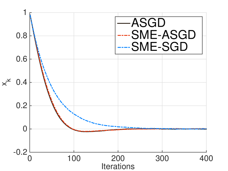
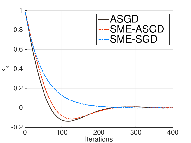
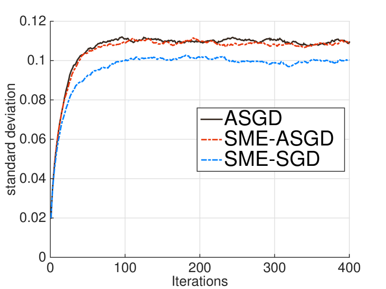
Figure 1: *

$\mu=0.9$

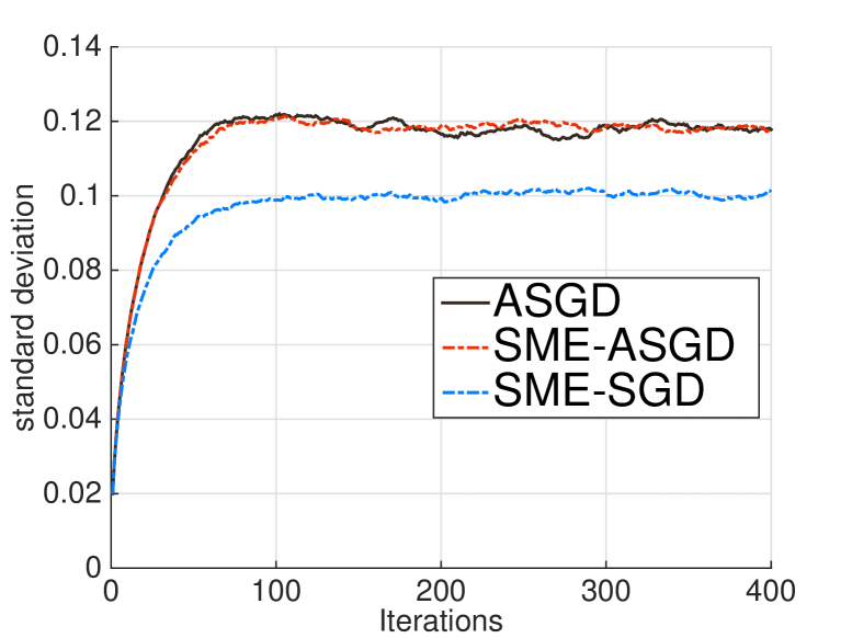
Figure 2: *

$\mu=0.95$

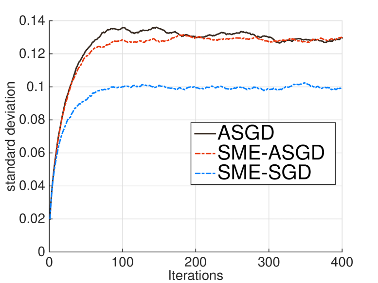
Figure 3: *

$\mu=0.97$

Figure 4: Apply the SME-ASGD to minimize the quadratic function $f(x)=x^{2}$ in different $\mu$’s, with two components $f_{1}(x)=(x-1)^{2}-1$, and $f_{2}(x)=(x+1)^{2}-1$. $x_{0}=1$ and $\eta=1e-2$. SME-ASGD achieves more accurate approximations compared to SME-SGD (3.3), especially when $\mu$ becomes large. However, one can also observe that when $\mu$ increases the error of the SME-ASGD approximation increases as well.

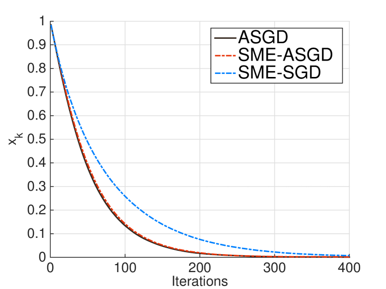
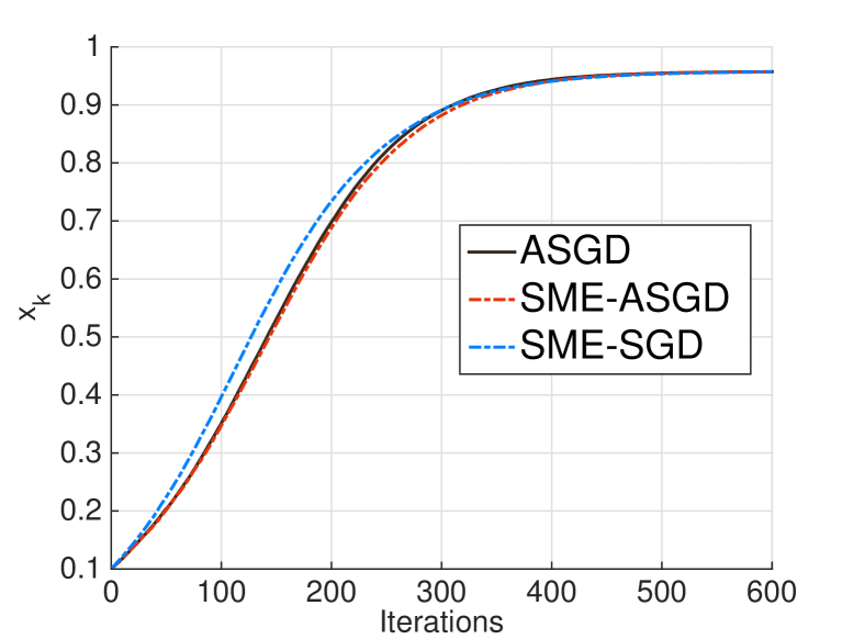
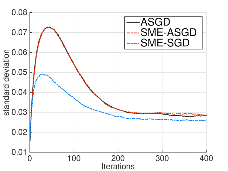
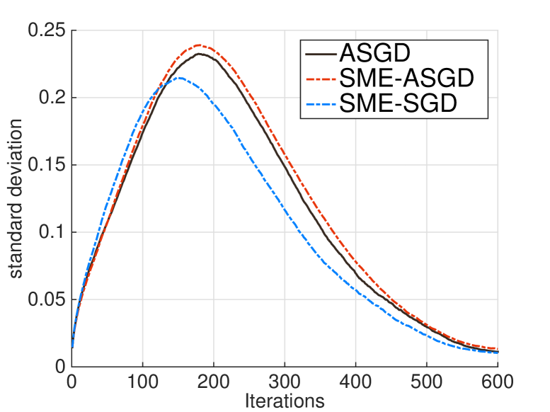
Figure 5: (Left) Apply the SME-ASGD to minimize the convex function $f(x)=x^{4}+6x^{2}$ with two components $f_{1}(x)=(x-1)^{4}-1$, and $f_{2}(x)=(x+1)^{4}-1$. Notice that the gradients are Lipschitz locally. Here we choose $x_{0}=1$, and a smaller step size $\eta=1e-3$. (Right) Apply the SME-ASGD to minimize the double well potential $f(x)=1-e^{-(x-1)^{2}}-e^{-(x+1)^{2}}$. Here $f_{1}=1-2e^{-(x-1)^{2}},f_{2}=1-2e^{-(x+1)^{2}}$ and both have Lipschitz gradients. We choose $\eta=1e-2,x_{0}=0.1$. Note that $\operatorname*{arg\,min}f(x)\approx\pm 0.9575$. In our case, due to the initial data $x_{0}$, $90.34\%$ of ASGD path samples converge to $0.9575$, while $90.50\%$ of SME-ASGD and $88.54\%$ of SME-SGD converge to the same minimizer. For both columns of numerical tests, we choose $\mu=0.95$.

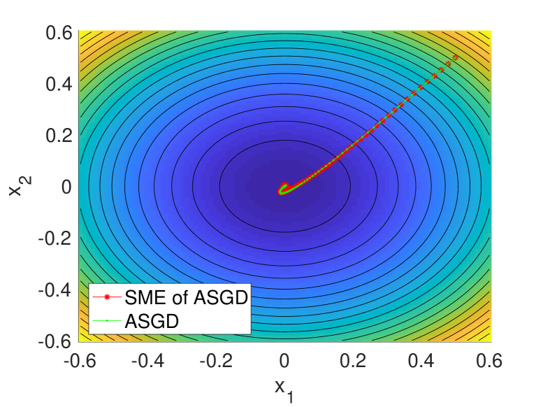
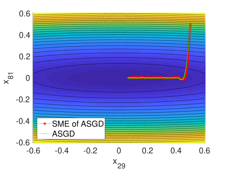
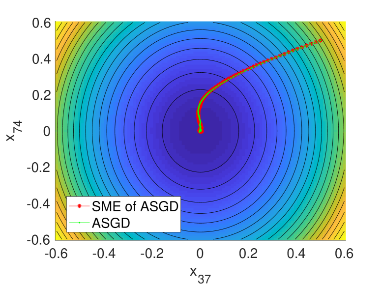
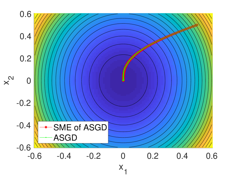
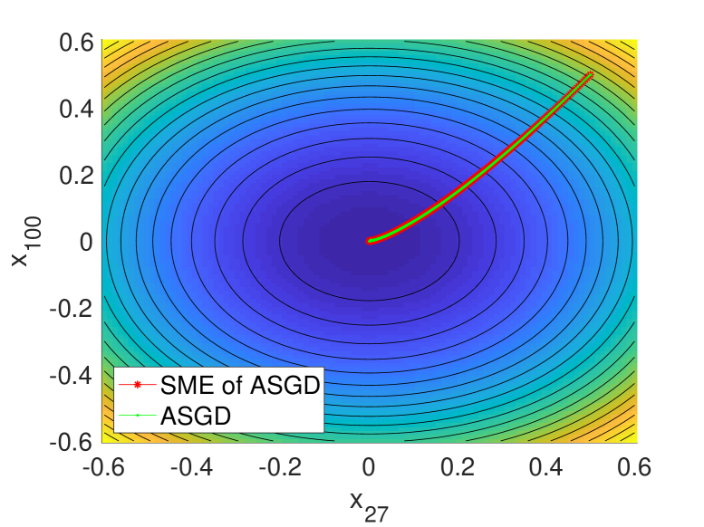
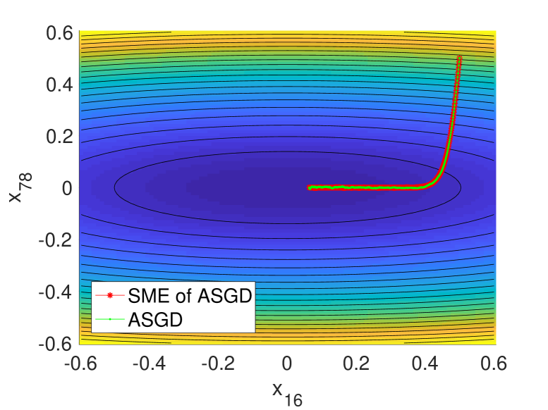
Figure 6: Apply the SME-ASGD to minimize the quadratic function $f(x)=\sum_{i=1}^{100}c_{i}x_{i}^{2}/2,~{}x\in\mathbb{R}^{100}$ with $\mu=0.90$ and two components $f_{1}(x)=\sum_{i=1}^{100}c_{i}x_{i}^{2}/2-x$, and $f_{2}(x)=\sum_{i=1}^{100}c_{i}x_{i}^{2}/2+x$. The initial condition $x_{0}=(0.5,0.5,\cdots,0.5)\in\mathbb{R}^{100}$ and the step size is $\eta=1e-2$. The plots are done after $1000$ iterations. The corresponding coefficients in the plots are $c_{1}=4.2593,c_{2}=4.9013,c_{29}=0.1980,c_{81}=4.3968,c_{37}=3.9978,c_{74}=1.9527$.

Figure 7: Apply the SME-ASGD to minimize the convex function $f(x)=\sum_{i=1}^{100}c_{i}(x_{i}^{4}+6x_{i}^{2})/2,~{}x\in\mathbb{R}^{100}$ with $\mu=0.90$ and two components $f_{1}(x)=\sum_{i=1}^{100}c_{i}(x_{i}-1)^{4}/2-1$, and $f_{2}(x)=\sum_{i=1}^{100}c_{i}(x_{i}+1)^{4}/2+1$. The initial condition $x_{0}=(0.5,0.5,\cdots,0.5)\in\mathbb{R}^{100}$ and the step size is $\eta=1e-3$. The plots are done after $1000$ iterations. The corresponding coefficients in the plots are $c_{1}=3.9212,c_{2}=1.9370,c_{27}=1.2093,c_{100}=1.5661,c_{16}=0.3353,c_{78}=4.5502$.

4 Optimal mini-batch size of ASGD

With much better understanding of dynamics of the ASGD algorithm using SME-ASGD, we are able to tune multiple hyper-parameters of ASGD using the predictions obtained from applying the stochastic optimal control theory to SME-ASGD. Here we demonstrate one such application: the optimal time-dependent mini-batch size for ASGD. By denoting the time-dependent batch size as $1+u_{k}$ with $u_{k}\geq 0$, one can write the iteration as

$$x_{k+1}=x_{k}-\eta\frac{1}{1+u_{k}}\sum_{j=1}^{1+u_{k}}\nabla f_{\gamma_{j}}(x_{k-\tau_{k}}).$$ (4.1)

We argue that it is reasonable to assume that the choice of mini-batch size is independent from $\gamma_{j}$ and the staleness $\tau_{k}$. This is because, even though changing the batch size will simultaneously change the "clocks" of all the processors, the staleness would not be changed as all the processors are impacted equally. Following the argument given in Section 2, we can derive a corresponding SME

$$dY_{t}=-\nabla f(X_{t})dt-\sqrt{\frac{1-\mu}{\eta}}Y_{t}dt$$

$$dX_{t}=Y_{t}dt+\frac{\sigma(t)\eta^{3/4}}{(1+u(t))^{1/2}(1-\mu)^{1/4}}dB_{t}.$$ (4.2)

The derivation here is not much different from the one of SME-ASGD (2.11), except for identifying the right coefficient in front of the the noise term $dB_{t}$. The correct coefficient (denoted by $c$ in the discussion below) is constrained by the following constraints on the variance

$$\mathbb{E} \left\{\frac{\eta^{2}}{(1+u_{k})^{2}}\left(\sum_{j=1}^{1+u_{k}}(-\frac{y_{k}}{\alpha}-\nabla f_{\gamma_{j}}(x_{k-\tau_{k}})\right)\left(\sum_{j=1}^{1+u_{k}}(-\frac{y_{k}}{\alpha}-\nabla f_{\gamma_{j}}(x_{k-\tau_{k}})\right)^{T}\right\}$$

$$=\frac{\eta^{2}}{(1+u_{k})^{2}}\sum_{j=1}^{1+u_{k}}\mathbb{E}\left\{\left(-\frac{y_{k}}{\alpha}-\nabla f_{\gamma_{j}}(x_{k-\tau_{k}})\right)\left(-\frac{y_{k}}{\alpha}-\nabla f_{\gamma_{j}}(x_{k-\tau_{k}})\right)^{T}\right\}=\frac{\eta^{2}}{1+u_{k}}\Sigma_{k}\sim c^{2}\Delta t,$$

where the cross terms vanish under the expectation. Plugging in $\Delta t=\sqrt{\eta(1-\mu)}$ shows that the coefficient for the noise is

$$c=\frac{\sigma(t)\eta^{3/4}}{(1+u(t))^{1/2}(1-\mu)^{1/4}}$$

as shown in (4).

We would like to explore the dynamics of SME to find the dominating eigenvalue for later use. To simplify the discussion, let us consider for example the quadratic loss objective $f(x)=x^{2}$. By applying the Ito’s formula to this SME, one obtains the following evoluation system for the second moments

$$\frac{d}{dt}\begin{bmatrix}\mathbb{E}(X_{t}^{2})\\ \mathbb{E}(Y_{t}^{2})\\ \mathbb{E}(X_{t}Y_{t})\end{bmatrix} =-\begin{bmatrix}0&0&-2\\ 0&2\sqrt{(1-\mu)/\eta}&4\\ 2&-1&\sqrt{(1-\mu)/\eta}\end{bmatrix}\begin{bmatrix}\mathbb{E}(X_{t}^{2})\\ \mathbb{E}(Y_{t}^{2})\\ \mathbb{E}(X_{t}Y_{t})\end{bmatrix}+\begin{bmatrix}\frac{\Sigma(t)\eta^{3/2}}{(1+u(t))(1-\mu)^{1/2}}\\ 0\\ 0\end{bmatrix}.$$ (4.3)

A similar derivation is shown in Appendix B, and we just replace all $\Sigma$ by $\Sigma/(1+u(t))$ in the mini-batching case. Here, we make a simplifying but practical assumption that $u(t)$ varies slowly. Now by freezing $u(t)$ to a constant $u$, (4.3) is a linear system with constant coefficients, its asymptotic behavior is determined by the eigenvalue of the coefficient matrix. An easy calculation shows that the eigenvalue with largest real part is given by $\lambda=-\sqrt{\nicefrac{{(1-\mu)}}{{\eta}}}+\sqrt{\nicefrac{{(1-\mu-8\eta)}}{{\eta}}}$ with a negative real part and therefore the second moment of $X_{t}$ decays exponentially. Moreover, (4.3) provides us with the stationary solution for $X^{2}$

$$z_{\infty}:=\mathbb{E}(X_{\infty}^{2})=\frac{\Sigma\eta}{2(1+u(t))}\Bigl{(}\frac{\eta}{1-\mu}+\frac{1}{2}\Bigr{)}.$$ (4.4)

For a slowly varying $u(t)$, $z_{\infty}=z_{\infty}(u(t))$ is a function of $u(t)$. Based on this simplication, rather than applying the optimal control subject to the full second moment equation, we shall work with a simpler evolution equation that asymptotically approximates the dynamics (imposed as a constraint). More specifically, we pose the following optimal control problem for the time-dependent mini-batch size

$$\min_{u\in\mathcal{A}}\bigg{\{}z(T)+\frac{\gamma}{\eta}\int_{0}^{T}u(s)ds\bigg{\}}\,\,\,\,\,\text{ subject to }$$ (4.5)

$$\frac{d}{dt}z(t)=\mathrm{Re}(\lambda)(z(t)-z_{\infty}(u(t)))\qquad\text{ with }z(0)=x_{0}^{2},$$

where $z(t)$ models $\mathbb{E}(X_{t}^{2})$ – the quantity to minimize, $\mathcal{A}=\{u(t)\geq 0\}$ is an admissible control set as the mini-batch size is greater than $1$, and $\gamma>0$ is a constant measuring the unit cost for introducing extra gradient samples throughout the time. Below we show how to solve the optimal control problem (4.5). The value function can be defined as

$$V(z,t)=\min_{u\in\mathcal{A}}\bigg{\{}z(T)+\frac{\gamma}{\eta}\int_{t}^{T}u(s)ds\;\bigg{|}\;\frac{d}{dt}z(t)=F(u(t),z(t)),z(t)=z\bigg{\}},$$ (4.6)

where $F(u(t),z(t))=\text{Re}(\lambda)(z(t)-z_{\infty}(u(t)))=\text{Re}(\lambda)\bigl{(}z(t)-\frac{\Sigma\eta}{2(1+u(t))}(\frac{\eta}{1-\mu}+\frac{1}{2})\bigr{)}$. The corresponding Hamilton-Jacobi-Bellman equation is

$$V_{t}+\min_{u\in\mathcal{A}}\bigg{\{}F(u,z)V_{z}+\frac{\gamma}{\eta}u\bigg{\}}=0$$ (4.7)

$$\text{with }V(0,t)=0,V(z,T)=z.$$

Since $\min_{u\in\mathcal{A}}\bigg{\{}F(u,z)V_{z}+\frac{\gamma}{\eta}u\bigg{\}}=\min_{u\in\mathcal{A}}\bigg{\{}\frac{-V_{z}\text{Re}(\lambda)\Sigma\eta}{2(1+u)}\big{(}\frac{\eta}{1-\mu}+\frac{1}{2}\big{)}+\frac{\gamma}{\eta}u\bigg{\}}$, $V_{z}\geq 0$, and $\text{Re}(\lambda)<0$, the minimum could be obtained by solving the following equation

$$\frac{V_{z}\text{Re}(\lambda)\Sigma\eta}{2(1+u)^{2}}\big{(}\frac{\eta}{1-\mu}+\frac{1}{2}\big{)}+\frac{\gamma}{\eta}=0$$

with the derivative of the value function $V_{z}$ to be determined later. Therefore the optimal batch size $u^{*}$ as a function of $V_{z}$ is

$$u^{*}(V_{z})=\begin{cases}\sqrt{\frac{-V_{z}\text{Re}(\lambda)\Sigma\eta^{2}}{2\gamma}\big{(}\frac{\eta}{1-\mu}+\frac{1}{2}\big{)}}-1&\text{if }\frac{-V_{z}\text{Re}(\lambda)\Sigma\eta^{2}}{2\gamma}\big{(}\frac{\eta}{1-\mu}+\frac{1}{2}\big{)}>1,\\ 0&\text{otherwise}.\end{cases}$$ (4.8)

The next step is to solve $V$ to get an explicit formula for $u^{*}$. Placing $u^{*}(V_{z})$ back into the minimization bracket, we obtain

$$\min_{u\in\mathcal{A}}\bigg{\{}F(u,z)V_{z}+\frac{\gamma}{\eta}u\bigg{\}}=\begin{cases}\text{Re}(\lambda)zV_{z}-\frac{\gamma}{\eta}&\text{if }\frac{-V_{z}\text{Re}(\lambda)\Sigma\eta^{2}}{2\gamma}\big{(}\frac{\eta}{1-\mu}+\frac{1}{2}\big{)}>1,\\ \text{Re}(\lambda)\big{(}z-\frac{\Sigma\eta}{2}\big{(}\frac{\eta}{1-\mu}+\frac{1}{2}\big{)}\big{)}V_{z}&\text{otherwise}.\end{cases}$$ (4.9)

This gives the Hamilton-Jacobi equation and we can solve it by using the method of characteristics. Letting $\gamma^{*}=-\frac{\text{Re}(\lambda)\Sigma\eta^{2}}{2}\big{(}\frac{\eta}{1-\mu}+\frac{1}{2}\big{)}$ for notation convenience, we obtain the solution for $V$

$$V(z,t)=\begin{cases}\frac{\Sigma\eta}{2}\big{(}\frac{\eta}{1-\mu}+\frac{1}{2}\big{)}+\big{(}z-\frac{\Sigma\eta}{2}\big{(}\frac{\eta}{1-\mu}+\frac{1}{2}\big{)}\big{)}e^{\text{Re}(\lambda)(T-t)}&\text{if }\gamma>\gamma^{*}\\ \big{(}z-\frac{\Sigma\eta}{2}\big{(}\frac{\eta}{1-\mu}+\frac{1}{2}\big{)}\big{)}e^{\text{Re}(\lambda)(T-t)}-\frac{\gamma}{\eta}(t^{*}+\frac{1}{\text{Re}(\lambda)})&\text{if }\gamma\leq\gamma^{*},0\leq t\leq T-t^{*}\\ ze^{\text{Re}(\lambda)(T-t)}-\frac{\gamma}{\eta}(T-t)&\text{if }\gamma\leq\gamma^{*},T-t^{*}<t\leq T,\end{cases}$$ (4.10)

where $t^{*}=\frac{1}{\text{Re}(\lambda)}\log(\frac{\gamma}{\gamma^{*}})$. For all cases, $V_{z}=e^{\text{Re}(\lambda)(T-t)}$. With this inserted back into (4.8), we conclude that

$$u^{*}(t)=\begin{cases}0&\text{if }\gamma>\gamma^{*}\text{ or }0\leq t\leq T-t^{*}\\ \sqrt{\frac{\gamma^{*}}{\gamma}}e^{\text{Re}(\lambda)(T-t)/2}-1&\text{if }\gamma\leq\gamma^{*},T-t^{*}<t\leq T.\end{cases}$$ (4.11)

In particular, (4.11) tells that we should use a small mini-batch size (even size $1$) during the early time (for $k\leq k^{*}=(T-t^{*})/\eta$), since during this period the gradient flow dominates the dynamics. After the transition time $k^{*}$ at which the noise starts to dominate, one shall apply mini-batch with size exponentially increasing in $k$ to reduce the variance. Figure 8 demonstrates that our proposed mini-batching strategy outperforms the ASGD with a constant batch size (for example, applied in [4, 7]). Note that such strategy of increasing the batch size in later stage of training has been also suggested and used in recent works in training large neural networks, e.g., [8, 10].

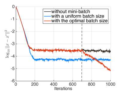
Figure 8: A comparison of performance in terms of $l^{2}$ error. We apply mini-batching over $n=100$ components $f_{i}(x)=\frac{1}{2}(x-c_{i})^{2},c_{i}=-1/2+i/(2n)$. Here we choose the step size $\eta=0.02$ and the initial data $x_{0}=1$. The batch size for the uniform mini-batching case is $5$. For the optimal mini-batching strategy, the transition happens at $k=(T-t^{*})/\eta\approx 699$, and the optimized batch size at time $T$ is $42$. In practice, we can apply a more aggressive mini-batching strategy by starting to increase the batch size earlier in the flat region, and it will result in a larger batch size at $T$.

5 Conclusion

In this paper, we have developed stochastic modified equations (SMEs) to model the asynchronous stochastic gradient descent (ASGD) algorithms in the continuous-time limit. For quadratic loss functions, the resulting SME can be put into a Langevin equation with a solution known to converge to the unique invariant measure with a convergence rate dictated by the corresponding temperature. We utilize such information to compare with the momentum SGD and prove the “asynchrony begets momentum” phenomenon. For the general case, though the resulting SME does not have an explicitly known invariant measure, it still provides rather precise trajectory predictions for the discrete ASGD dynamics. Moreover, with SME available, we are able to find optimal hyper-parameters for ASGD algorithms by performing a moment analysis and leveraging the optimal control theory.

Funding

J.A. is partially supported by the Gene Golub Research Fellowship. J.L. is supported by the National Science Foundation under award DMS-1454939, and L.Y. is partially supported by the U.S. Department of Energy, Office of Science, Office of Advanced Scientific Computing Research, Scientific Discovery through Advanced Computing (SciDAC) program and the National Science Foundation under award DMS-1818449.

Appendix A: miscellaneous computations in SMEs

In this section, we provide the missing computations in Section 2.

5.1 Evolution equation of $\Sigma$ for nonlinear gradients

First, we have

$$\Sigma_{k} =\mathbb{E}\bigg{(}(-\frac{y_{k}}{\alpha}-\nabla f_{\gamma_{k}}(x_{k-\tau_{k}}))(-\frac{y_{k}}{\alpha}-\nabla f_{\gamma_{k}}(x_{k-\tau_{k}}))^{T}\bigg{)}.$$

By expanding the terms in the expectation and treating them individually, we arrive at the following

$$\Sigma_{k} =\frac{1}{\alpha^{2}}y_{k}y_{k}^{T}+\frac{y_{k}}{\alpha}\mathbb{E}\{\nabla f_{\gamma_{k}}(x_{k-\tau_{k}})^{T}\}+\mathbb{E}\{\nabla f_{\gamma_{k}}(x_{k-\tau_{k}})\}\frac{y_{k}^{T}}{\alpha}+\mathbb{E}\{\nabla f_{\gamma_{k}}(v_{k})\nabla f_{\gamma_{k}}(x_{k-\tau_{k}})^{T}\}$$ (5.1)

$$=\mathbb{E}\{\nabla f_{\gamma_{k}}(x_{k-\tau_{k}})\nabla f_{\gamma_{k}}(x_{k-\tau_{k}})^{T}\}-\frac{1}{\alpha^{2}}y_{k}y_{k}^{T}$$

$$=\mu\sum_{m=0}^{\infty}\mathbb{E}\{\nabla f_{\gamma_{k-1}}(x_{k-1-m})\nabla f_{\gamma_{k-1}}(x_{k-1-m})^{T}\}(1-\mu)\mu^{m}$$

$$\,\,\,\,+(1-\mu)\mathbb{E}\{\nabla f_{\gamma_{k}}(x_{k})\nabla f_{\gamma_{k}}(x_{k})^{T}\}-\frac{1}{\alpha^{2}}y_{k}y_{k}^{T}$$

$$=\mu\big{(}\Sigma_{k-1}+\frac{1}{\alpha^{2}}y_{k-1}y_{k-1}^{T}\big{)}+(1-\mu)\mathbb{E}\{\nabla f_{\gamma_{k}}(x_{k})\nabla f_{\gamma_{k}}(x_{k})^{T}\}-\frac{1}{\alpha^{2}}y_{k}y_{k}^{T}$$

$$=\mu\big{(}\Sigma_{k-1}+\frac{1}{\alpha^{2}}y_{k-1}y_{k-1}^{T}\big{)}+\frac{1-\mu}{n}\sum_{i=1}^{n}\nabla f_{i}(x_{k})\nabla f_{i}(x_{k})^{T}-\frac{1}{\alpha^{2}}y_{k}y_{k}^{T}.$$

Notice that $y_{k}=\mu y_{k-1}-\alpha(1-\mu)\nabla f(x_{k})$, and thus we have

$$y_{k-1}y_{k-1}^{T} =\frac{1}{\mu^{2}}\big{(}y_{k}+\alpha(1-\mu)\nabla f(x_{k})\big{)}\big{(}y_{k}+\alpha(1-\mu)\nabla f(x_{k})\big{)}^{T}$$

$$=\frac{1}{\mu^{2}}\bigg{(}y_{k}y_{k}^{T}+\alpha(1-\mu)y_{k}\nabla f(x_{k})^{T}+\alpha(1-\mu)\nabla f(x_{k})y_{k}^{T}+\alpha^{2}(1-\mu)^{2}\nabla f(x_{k})\nabla f(x_{k})^{T}\bigg{)}.$$

Substituting it in (5.1), we obtain

$$\frac{\Sigma_{k}-\Sigma_{k-1}}{\alpha(1-\mu)}= -\frac{1}{\alpha}\Sigma_{k-1}+\frac{1}{\alpha^{3}\mu}y_{k}y_{k}^{T}+\frac{1}{\alpha^{2}\mu}y_{k}\nabla f(x_{k})^{T}+\frac{1}{\alpha^{2}\mu}\nabla f(x_{k})y_{k}^{T}$$

$$+\frac{1-\mu}{\alpha\mu}\nabla f(x_{k})\nabla f(x_{k})^{T}+\frac{1}{\alpha n}\sum_{i=1}^{n}\nabla f_{i}(x_{k})\nabla f_{i}(x_{k})^{T}.$$

Using this and $\Delta t=\alpha(1-\mu),\alpha=\sqrt{\frac{\eta}{1-\mu}}$, we obtain the evolution equation (2.12).

5.2 Evolution equation of $\Sigma$ for linear gradients

Similar to section 5.1, we have

$$\Sigma_{k} =\mathbb{E}\bigl{(}(\nabla f(m_{k})-\nabla f_{\gamma_{k}}(x_{k-\tau_{k}}))(\nabla f(m_{k})-\nabla f_{\gamma_{k}}(x_{k-\tau_{k}}))^{T}\bigr{)}$$

$$=\mu(\Sigma_{k-1}+\nabla f(m_{k-1})\nabla f(m_{k-1})^{T})+(1-\mu)\mathbb{E}(\nabla f_{\gamma_{k}}(x_{k})\nabla f_{\gamma_{k}}(x_{k})^{T})-\nabla f(m_{k})\nabla f(m_{k})^{T}.$$ (5.2)

We then subtract both sides by $\Sigma_{k-1}$ and divide by $\Delta t=\sqrt{\eta(1-\mu)}$. Moreover, we use the relation

$$x_{k}=\frac{m_{k}-\mu m_{k-1}}{1-\mu}=\frac{m_{k}-\mu(m_{k}-p_{k}\Delta t)}{1-\mu}=m_{k}+\mu\sqrt{\frac{\eta}{1-\mu}}p_{k}$$

to replace $x_{k}$ in (5.2), and replace $m_{k-1}$ by $m_{k}-p_{k}\Delta t$. Then, since the gradient of $f$ is linear, rearrange the terms we get

$$\frac{\Sigma_{k}-\Sigma_{k-1}}{\sqrt{\eta(1-\mu)}}= -\sqrt{\frac{1-\mu}{\eta}}\Sigma_{k-1}-\sqrt{\frac{1-\mu}{\eta}}\nabla f(m_{k})\nabla f(m_{k})^{T}+\mu\sqrt{\eta(1-\mu)}\nabla f(p_{k})\nabla f(p_{k})^{T}$$

$$-\mu(\nabla f(m_{k})\nabla f(p_{k})^{T} +\nabla f(p_{k})\nabla f(m_{k})^{T})+\frac{1}{n}\sqrt{\frac{1-\mu}{\eta}}\sum_{i=1}^{n}\nabla f_{i}(m_{k}+\mu\sqrt{\frac{\eta}{1-\mu}}p_{k})\nabla f_{i}(m_{k}+\mu\sqrt{\frac{\eta}{1-\mu}}p_{k})^{T}.$$

5.3 SME for SGD with momentum

Recall the iteration for the SGD with a constant momentum parameter is

$$v_{k+1}=\mu^{\prime}v_{k}-\eta^{\prime}\nabla f_{\gamma_{k}}(x_{k})$$

$$x_{k+1}=x_{k}+v_{k+1},$$

which can be viewed as a second-order difference equation. To ensure the final equation with all terms of order $O(1)$, one needs $\eta^{\prime}=(\Delta t)^{2}$. We can rewrite (2.6) as

$$\frac{v_{k+1}}{\sqrt{\eta^{\prime}}}=\frac{v_{k}}{\sqrt{\eta^{\prime}}}+\sqrt{\eta^{\prime}}\bigg{(}-\frac{1-\mu^{\prime}}{\eta^{\prime}}v_{k}-\nabla f(x_{k})\bigg{)}+\sqrt{\eta^{\prime}}(\nabla f(x_{k})-\nabla f_{\gamma_{k}}(x_{k}))$$

$$x_{k+1}=x_{k}+\frac{v_{k+1}}{\sqrt{\eta^{\prime}}}\sqrt{\eta^{\prime}}.$$ (5.3)

Let us introduce $p=v/\sqrt{\eta^{\prime}}$. In order to have $\sqrt{\eta^{\prime}}(\nabla f(x_{k})-\nabla_{\gamma_{k}}f(x_{k}))\sim c\Delta B_{t}$, we choose $c\sim\sigma(\eta^{\prime})^{1/4}$. Therefore, we obtain the first order weak approximation, which can also be viewed as the Euler-Maruyama discretization of the following SDE

$$dP_{t}=-\nabla f(X_{t})dt-\frac{1-\mu^{\prime}}{\sqrt{\eta^{\prime}}}P_{t}dt+\sigma(X_{t})(\eta^{\prime})^{\frac{1}{4}}dB_{t}$$

$$dX_{t}=P_{t}dt.$$

Appendix B: dynamics of SME-ASGD (2.11)

We consider the one dimensional case with $f(x)=\frac{1}{2}ax^{2}$. The goal here is to give an analysis of the dynamics of first and second moment of $X$ and $Y$ under (2.11). Taking expectation, we obtain

$$d\begin{bmatrix}\mathbb{E}(Y_{t})\\ \mathbb{E}(X_{t})\end{bmatrix}=\begin{bmatrix}-\sqrt{\frac{1-\mu}{\eta}}&-a\\ 1&0\end{bmatrix}\begin{bmatrix}\mathbb{E}(Y_{t})\\ \mathbb{E}(X_{t})\end{bmatrix}dt=A(\mu,\eta)\begin{bmatrix}\mathbb{E}(Y_{t})\\ \mathbb{E}(X_{t})\end{bmatrix}dt.$$

One observes that the eigenvalues of $A(\mu,\eta)$ are $\lambda_{1,2}(A)=\frac{1}{2}\bigg{(}-\sqrt{\frac{1-\mu}{\eta}}\pm\sqrt{\frac{1-\mu}{\eta}-4a}\bigg{)}$, the real parts of both are negative as long as $a>0$. From this, we conclude that, when $a>0$, the expectation of $X_{t}$ decays exponentially. The corresponding stationary solutions are given by

$$\mathbb{E}(X_{\infty})=\mathbb{E}(Y_{\infty})=0.$$

For the second moment, we end up with the following equations by using the Ito’s formula

$$d\mathbb{E}(X_{t}^{2})=2\mathbb{E}(X_{t}Y_{t})dt+\Sigma(t)\frac{\eta^{3/2}}{(1-\mu)^{1/2}}dt$$

$$d\mathbb{E}(Y_{t}^{2})=-2a\mathbb{E}(X_{t}Y_{t})dt-2\sqrt{\frac{1-\mu}{\eta}}\mathbb{E}(Y_{t}^{2})dt$$

$$d\mathbb{E}(X_{t}Y_{t})=-a\mathbb{E}(X_{t}^{2})dt+\mathbb{E}(Y_{t}^{2})dt-\sqrt{\frac{1-\mu}{\eta}}\mathbb{E}(X_{t}Y_{t})dt.$$ (5.4)

In order to study the behavior of the second moments, we can rewrite (Appendix B: dynamics of SME-ASGD (2.11)) as

$$d\begin{bmatrix}\mathbb{E}(X_{t}^{2})\\ \mathbb{E}(Y_{t}^{2})\\ \mathbb{E}(X_{t}Y_{t})\end{bmatrix} =\begin{bmatrix}0&0&2\\ 0&-2\sqrt{\frac{1-\mu}{\eta}}&-2a\\ -a&1&-\sqrt{\frac{1-\mu}{\eta}}\end{bmatrix}\begin{bmatrix}\mathbb{E}(X_{t}^{2})\\ \mathbb{E}(Y_{t}^{2})\\ \mathbb{E}(X_{t}Y_{t})\end{bmatrix}dt+\begin{bmatrix}\Sigma(t)\frac{\eta^{3/2}}{(1-\mu)^{1/2}}\\ 0\\ 0\end{bmatrix}dt.$$ (5.5)

The corresponding stationary solutions are

$$\mathbb{E}(X_{\infty}Y_{\infty})=\frac{-\Sigma\eta^{3/2}}{2(1-\mu)^{1/2}},\,\,\mathbb{E}(Y_{\infty}^{2})=\frac{a\Sigma\eta^{2}}{2(1-\mu)},\,\text{ and }\mathbb{E}(X_{\infty}^{2})=\frac{\Sigma\eta^{2}}{2(1-\mu)}+\frac{\Sigma\eta}{2a}.$$

Let us introduce

$$B(\mu,\eta)=\begin{bmatrix}0&0&2\\ 0&-2\sqrt{\frac{1-\mu}{\eta}}&-2a\\ -a&1&-\sqrt{\frac{1-\mu}{\eta}}\end{bmatrix}.$$

The eigenvalues of $B(\mu,\eta)$ are

$$\lambda_{1}=-\sqrt{\frac{1-\mu}{\eta}},\lambda_{2,3}=\lambda_{\pm}=-\sqrt{\frac{1-\mu}{\eta}}\pm\sqrt{\frac{1-\mu}{\eta}-4a}.$$

We can see that the real parts of all roots are negative as long as $a>0$. Moreover, the second moment of $X_{t}$ decays exponentially, with the rate given by $\mathrm{Re}(\lambda_{+})$ since $\lambda_{+}$ is the eigenvalue with the largest (negative) real part. We obtain the largest descent rate $\mathrm{Re}(\lambda_{+})$ when the second part $\sqrt{\frac{1-\mu}{\eta}-4a}$ in $\lambda_{+}$ is purely imaginary, i.e., when $\mu$ takes

$$\mu_{\text{opt}}=\max\{1-4a\eta,0\}.$$ (5.6)

We note that (5.6) also gives a suggestion to choose optimal step size $\eta$: when $\mu$ is given, the maximal step size we can choose is $\eta_{\text{opt}}=\frac{1-\mu}{4a}$. Any step size beyond that will cause oscillations in the SME and the corresponding ASGD.

References

- [1] A. Agarwal and J.C. Duchi. Distributed delayed stochastic optimization. In Advances in Neural Information Processing Systems, pages 873–881, 2011.
- [2] Serge Bernstein. Sur les fonctions absolument monotones. Acta Math., 52:1–66, 1929.
- [3] L. Bottou, F.E. Curtis, and J. Nocedal. Optimization methods for large-scale machine learning, 2016. preprint, arXiv:1606.04838.
- [4] O. Dekel, R. Gilad-Bachrach, O. Shamir, and L. Xiao. Optimal distributed online prediction using mini-batches. Journal of Machine Learning Research, 13(Jan):165–202, 2012.
- [5] J.C. Duchi, E. Hazan, and Y. Singer. Adaptive subgradient methods for online learning and stochastic optimization. Journal of Machine Learning Research, 12(Jul):2121–2159, 2011.
- [6] J.C. Duchi, M.I. Jordan, and B. McMahan. Estimation, optimization, and parallelism when data is sparse. In Advances in Neural Information Processing Systems, pages 2832–2840, 2013.
- [7] K. Gimpel, D. Das, and N.A. Smith. Distributed asynchronous online learning for natural language processing. In Proceedings of the Fourteenth Conference on Computational Natural Language Learning, pages 213–222. Association for Computational Linguistics, 2010.
- [8] P. Goyal, P. Dollár, R. Girshick, P. Noordhuis, L. Wesolowski, A. Kyrola, A. Tulloch, Y. Jia, and K. He. Accurate, large minibatch SGD: Training ImageNet in 1 hour, 2017. arXiv preprint, arXiv:1706.02677.
- [9] M. Hardt, B. Recht, and Y. Singer. Train faster, generalize better: Stability of stochastic gradient descent. In International Conference on Machine Learning, pages 1225–1234, 2016.
- [10] N.S. Keskar, D. Mudigere, J. Nocedal, M. Smelyanskiy, and P. T. P. Tang. On large-batch training for deep learning: Generalization gap and sharp minima. In International Conference on Learning Representations, 2017.
- [11] D.P. Kingma and J. Ba. Adam: A method for stochastic optimization. International Conference on Learning Representations, 2015.
- [12] P.E. Kloeden and E. Platen. Stochastic differential equations. In Numerical Solution of Stochastic Differential Equations, pages 103–160. Springer, 1992.
- [13] Q. Li, C. Tai, and W. E. Stochastic modified equations and adaptive stochastic gradient algorithms. In International Conference on Machine Learning, pages 2101–2110, 2017.
- [14] J. Liu and S.J. Wright. Asynchronous stochastic coordinate descent: Parallelism and convergence properties. SIAM Journal on Optimization, 25(1):351–376, 2015.
- [15] J. Liu, S.J. Wright, C. Ré, V. Bittorf, and S. Sridhar. An asynchronous parallel stochastic coordinate descent algorithm. The Journal of Machine Learning Research, 16(1):285–322, 2015.
- [16] I. Mitliagkas, C. Zhang, S. Hadjis, and C. Ré. Asynchrony begets momentum, with an application to deep learning. In Communication, Control, and Computing (Allerton), 2016 54th Annual Allerton Conference on, pages 997–1004. IEEE, 2016.
- [17] D. Needell, R. Ward, and N. Srebro. Stochastic gradient descent, weighted sampling, and the randomized kaczmarz algorithm. In Advances in Neural Information Processing Systems, pages 1017–1025, 2014.
- [18] Y. Nesterov. Efficiency of coordinate descent methods on huge-scale optimization problems. SIAM Journal on Optimization, 22(2):341–362, 2012.
- [19] G.A. Pavliotis. Stochastic processes and applications: Diffusion processes, the Fokker-Planck and Langevin equations, volume 60. Springer, 2014.
- [20] B.T. Polyak. Some methods of speeding up the convergence of iteration methods. USSR Computational Mathematics and Mathematical Physics, 4(5):1–17, 1964.
- [21] B. Recht, C. Ré, S. Wright, and F. Niu. Hogwild: A lock-free approach to parallelizing stochastic gradient descent. In Advances in neural information processing systems, pages 693–701, 2011.
- [22] P. Richtárik and M. Takáč. Iteration complexity of randomized block-coordinate descent methods for minimizing a composite function. Mathematical Programming, 144(1-2):1–38, 2014.
- [23] I. Sutskever, J. Martens, G. Dahl, and G. Hinton. On the importance of initialization and momentum in deep learning. In International conference on machine learning, pages 1139–1147, 2013.
- [24] T. Tieleman and G. Hinton. Lecture 6.5-rmsprop: Divide the gradient by a running average of its recent magnitude. COURSERA: Neural networks for machine learning, 4(2):26–31, 2012.
- [25] HL Younes. Verification and Planning for Stochastic Processes with Asynchronous Events. PhD thesis, Academy of Engineering Sciences, 2005.