Fast and Accurate Binary Response Mixed Model

Analysis via Expectation Propagation

By P. Hall¹, I.M. Johnstone², J.T. Ormerod³, M.P. Wand⁴ and J.C.F. Yu⁴

¹University of Melbourne, ²Stanford University, ³University of Sydney

and ⁴University of Technology Sydney

22nd May, 2018

Abstract

Expectation propagation is a general prescription for approximation of integrals in statistical inference problems. Its literature is mainly concerned with Bayesian inference scenarios. However, expectation propagation can also be used to approximate integrals arising in frequentist statistical inference. We focus on likelihood-based inference for binary response mixed models and show that fast and accurate quadrature-free inference can be realized for the probit link case with multivariate random effects and higher levels of nesting. The approach is supported by asymptotic theory in which expectation propagation is seen to provide consistent estimation of the exact likelihood surface. Numerical studies reveal the availability of fast, highly accurate and scalable methodology for binary mixed model analysis.

Keywords: Best prediction; Generalized linear mixed models; Maximum likelihood; Kullback-Leibler projection; Message passing; Quasi-Newton methods; Scalable statistical methodology.

1 Introduction

Binary response mixed model-based data analysis is ubiquitous in many areas of application, with examples such as analysis of biomedical longitudinal data (e.g. Diggle et al., 2002), social science multilevel data (e.g. Goldstein, 2010), small area survey data (e.g. Rao & Molina, 2015) and economic panel data (e.g. Baltagi, 2013). The standard approach for likelihood-based inference in the presence of multivariate random effects is Laplace approximation, which is well-known to be inconsistent and prone to inferential inaccuracy. Our main contribution is to overcome this problem using expectation propagation. The new approach possesses speed and scalability on par with that of Laplace approximation, but is provably consistent and demonstrably very accurate. Bayesian approaches and Monte Carlo methods offer another route to accurate inference for binary response mixed models (e.g. Gelman & Hill, 2007). However, speed and scalability issues aside, frequentist inference is the dominant approach in many areas in which mixed models are used. Henceforth, we focus on frequentist binary mixed model analysis.

The main obstacle for likelihood-based inference for binary mixed models is the presence of irreducible integrals. For grouped data with one level of nesting, the dimension of the integrals matches the number of random effects. The two most common approaches to dealing with these integrals are (1) quadrature and (2) Laplace approximation. For example, in the R computing environment (R Core Team, 2018) the function glmer() in the package lme4 (Bates et al., 2015) supports both adaptive Gauss-Hermite quadrature and Laplace approximation for univariate random effects. For multivariate random effects only Laplace approximation is supported by glmer(), presumably because of the inherent difficulties of higher dimensional quadrature. Laplace approximation eschews multivariate integration via quadratic approximation of the log-integrand. However, the resultant approximate inference is well-known to be inaccurate, often to an unacceptable degree, in binary mixed models (e.g. McCulloch et al., Section 14.4). An embellishment of Laplace approximation, known as integrated nested Laplace approximation (Rue, Martino & Chopin, 2009), has been successful in various Bayesian inference contexts.

Expectation propagation (e.g. Minka, 2001) is general prescription for approximation of integrals that arise in statistical inference problems. Most of its literature is within the realm of Computer Science and, in particular, geared towards approximate inference for Bayesian graphical models (e.g. Chapter 10, Bishop, 2006). A major contribution of this article is transferral of expectation propagation methodology to frequentist statistical inference. In principle, our approach applies to any generalized linear mixed model situation. However, expectation propagation for binary response mixed model analysis has some especially attractive features and therefore we focus on this class of models. In the special case of probit mixed models, the expectation propagation approximation to the log-likelihood is exact regardless of the dimension of the random effects. This leads to a new practical alternative to multivariate quadrature. Moreover, asymptotic theory reveals that expectation propagation provides consistent approximation of the exact likelihood surface. This implies very good inferential accuracy of expectation propagation, and is supported by our simulation results. We are not aware of any other quadrature-free approaches to generalized mixed model analysis that has such a strong theoretical underpinning.

To facilitate widespread use of the new approach, a new package in the R language (R Core Team, 2018) has been launched. The package, glmmEP (Wand & Yu, 2018), uses a low-level language implementation of expectation propagation for speedy approximate likelihood-based inference and scales well to large sample sizes.

Binary response mixed models, and their inherent computational challenges, are summarized in Section 2 The expectation propagation approach to fitting and approximate inference, with special attention given to the quadrature-free probit link situation, is given in Section 3. Section 4 presents the results of numerical studies for both simulated and real data, and shows expectation propagation to be of great practical value as a fast, high quality approximation that scales well to big data and big model situations. Theoretical considerations are summarised in Section 5. Higher level and random effects extensions are touched upon in Section 6. Lastly, we briefly discuss transferral of new approach to other generalized linear mixed model settings in Section 7.

2 Binary Response Mixed Models

Binary mixed models for grouped data with one level of nesting and Gaussian random effects has the general form

$$y_{ij}|\boldsymbol{u}_{i}\stackrel{{\scriptstyle{\tiny\mbox{ind.}}}}{{\sim}}\mbox{Bernoulli}\big{(}F\big{(}\boldsymbol{\beta}^{T}\boldsymbol{x}^{\mbox{\tiny F}}_{ij}+\boldsymbol{u}_{i}^{T}\boldsymbol{x}^{\mbox{\tiny R}}_{ij}\big{)}\big{)},\quad\boldsymbol{u}_{i}\stackrel{{\scriptstyle{\tiny\mbox{ind.}}}}{{\sim}}N(\boldsymbol{0},\boldsymbol{\Sigma}),\quad 1\leq i\leq m,\quad 1\leq j\leq n_{i}$$ (1)

where $F$, the inverse link, is a pre-specified cumulative distribution function and $y_{ij}$ is the $j$th response for the $i$th group, where number of groups is $m$ and the number of responses measurements within the $i$th group is $n_{i}$. Also, $\boldsymbol{x}^{\mbox{\tiny F}}_{ij}$ is a $d^{\mbox{\tiny F}}\times 1$ vector of predictors corresponding to $y_{ij}$, modeled as having fixed effects with coefficient vector $\boldsymbol{\beta}$. Similarly, $\boldsymbol{x}^{\mbox{\tiny R}}_{ij}$ is a $d^{\mbox{\tiny R}}\times 1$ vector of predictors modeled as having random effects with coefficient vectors $\boldsymbol{u}_{i}$, $1\leq i\leq m$. Typically, $\boldsymbol{x}^{\mbox{\tiny R}}_{ij}$ is a sub-vector of $\boldsymbol{x}^{\mbox{\tiny F}}_{ij}$. It is also very common for each of $\boldsymbol{x}^{\mbox{\tiny R}}_{ij}$ and $\boldsymbol{x}^{\mbox{\tiny F}}_{ij}$ to have first entry equal to $1$, corresponding to fixed and random intercepts. The random effects covariance matrix $\boldsymbol{\Sigma}$ has dimension $d^{\mbox{\tiny R}}\times d^{\mbox{\tiny R}}$.

By far, the most common choices for $F$ are

$$F=\left\{\begin{array}[]{ll}\mbox{expit}&\mbox{for logistic mixed models}\\[4.30554pt] \Phi&\mbox{for probit mixed models}\\ \end{array}\right.$$

where $\mbox{expit}(x)\equiv 1/(1+e^{-x})$ and $\Phi$ is the cumulative distribution function of the $N(0,1)$ distribution.

Despite the simple form of (1), likelihood-based inference for the parameters $\boldsymbol{\beta}$ and $\boldsymbol{\Sigma}$ and best prediction of the random effects $\boldsymbol{u}_{i}$ is very numerically challenging. Assuming that $F(x)+F(-x)=1$, as is the case for the logistic and probit cases, the log-likelihood is

$$\ell(\boldsymbol{\beta},\boldsymbol{\Sigma})=\sum_{i=1}^{m}\log\int_{{\mathbb{R}}^{d^{\mbox{\tiny R}}}}\left\{\prod_{j=1}^{n_{i}}F\big{(}(2y_{ij}-1)(\boldsymbol{\beta}^{T}\boldsymbol{x}^{\mbox{\tiny F}}_{ij}+\boldsymbol{u}^{T}\boldsymbol{x}^{\mbox{\tiny R}}_{ij})\big{)}\right\}|2\pi\boldsymbol{\Sigma}|^{-1/2}\exp(-{\textstyle{\frac{1}{2}}}\boldsymbol{u}^{T}\boldsymbol{\Sigma}^{-1}\boldsymbol{u})\,d\boldsymbol{u}$$ (2)

and the best predictor of $\boldsymbol{u}_{i}$ is

$$\mbox{BP}(\boldsymbol{u}_{i})=\frac{\int_{{\mathbb{R}}^{d^{\mbox{\tiny R}}}}\boldsymbol{u}\left\{\prod_{j=1}^{n_{i}}F\big{(}(2y_{ij}-1)(\boldsymbol{\beta}^{T}\boldsymbol{x}^{\mbox{\tiny F}}_{ij}+\boldsymbol{u}^{T}\boldsymbol{x}^{\mbox{\tiny R}}_{ij})\big{)}\right\}\exp(-{\textstyle{\frac{1}{2}}}\boldsymbol{u}^{T}\boldsymbol{\Sigma}^{-1}\boldsymbol{u})\,d\boldsymbol{u}}{\int_{{\mathbb{R}}^{d^{\mbox{\tiny R}}}}\left\{\prod_{j=1}^{n_{i}}F\big{(}(2y_{ij}-1)(\boldsymbol{\beta}^{T}\boldsymbol{x}^{\mbox{\tiny F}}_{ij}+\boldsymbol{u}^{T}\boldsymbol{x}^{\mbox{\tiny R}}_{ij})\big{)}\right\}\exp(-{\textstyle{\frac{1}{2}}}\boldsymbol{u}^{T}\boldsymbol{\Sigma}^{-1}\boldsymbol{u})\,d\boldsymbol{u}},\quad 1\leq i\leq m.$$

The $d^{\mbox{\tiny R}}$-dimensional integrals in the $\ell(\boldsymbol{\beta},\boldsymbol{\Sigma})$ and $\mbox{BP}(\boldsymbol{u}_{i})$ expressions cannot be reduced further and multivariate numerical integration must be called upon for their evaluation. In addition, $\ell(\boldsymbol{\beta},\boldsymbol{\Sigma})$ has to be maximized over $\{d^{\mbox{\tiny F}}+{\textstyle{\frac{1}{2}}}\,d^{\mbox{\tiny R}}(d^{\mbox{\tiny R}}+1)\}$-dimensional space to obtain maximum likelihood estimates. Lastly, there is the problem of obtaining approximate confidence intervals for the entries of $\boldsymbol{\beta}$ and $\boldsymbol{\Sigma}$ and approximate prediction intervals for the entries of $\boldsymbol{u}_{i}$.

3 Expectation Propagation Likelihood Approximation

We will first explain expectation propagation for approximation of the log-likelihood $\ell(\boldsymbol{\beta},\boldsymbol{\Sigma})$. Approximation of $\mbox{BP}(\boldsymbol{u}_{i})$ follows relatively quickly. First note that $\ell(\boldsymbol{\beta},\boldsymbol{\Sigma})=\sum_{i=1}^{m}\ell_{i}(\boldsymbol{\beta},\boldsymbol{\Sigma})$ where

$$\ell_{i}(\boldsymbol{\beta},\boldsymbol{\Sigma})\equiv\log\int_{{\mathbb{R}}^{d^{\mbox{\tiny R}}}}\left\{\prod_{j=1}^{n_{i}}F\big{(}(2y_{ij}-1)(\boldsymbol{\beta}^{T}\boldsymbol{x}^{\mbox{\tiny F}}_{ij}+\boldsymbol{u}^{T}\boldsymbol{x}^{\mbox{\tiny R}}_{ij})\big{)}\right\}|2\pi\boldsymbol{\Sigma}|^{-1/2}\exp(-{\textstyle{\frac{1}{2}}}\boldsymbol{u}^{T}\boldsymbol{\Sigma}^{-1}\boldsymbol{u})\,d\boldsymbol{u}.$$

Each of the $\ell_{i}(\boldsymbol{\beta},\boldsymbol{\Sigma})$ are approximated individually and then summed to approximate $\ell(\boldsymbol{\beta},\boldsymbol{\Sigma})$ The essence is of the approximation of $\ell_{i}(\boldsymbol{\beta},\boldsymbol{\Sigma})$ is replacement of each

$$F\big{(}(2y_{ij}-1)(\boldsymbol{\beta}^{T}\boldsymbol{x}^{\mbox{\tiny F}}_{ij}+\boldsymbol{u}^{T}\boldsymbol{x}^{\mbox{\tiny R}}_{ij})\big{)},\quad 1\leq j\leq n_{i},$$

by an unnormalized Multivariate Normal density function, chosen according to an appropriate minimum Kullback-Leibler divergence criterion. The resultant integrand is then proportional to a product of Multivariate Normal density functions and admits an explicit form. The number approximating density functions of the same order of magnitude and, together with the properties of minimum Kullback-Leibler divergence, leads to accurate and statistically consistent approximation of $\ell(\boldsymbol{\beta},\boldsymbol{\Sigma})$. In probit case, where $F=\Phi$, the minimum Kullback-Leibler divergence steps are explicit. This leads to accurate approximation of $\ell(\boldsymbol{\beta},\boldsymbol{\Sigma})$ without the need for any numerical integration – just some fixed-point iteration. The expectation propagation-approximate log-likelihood, which we denote by $\underaccent{\sim}{\ell}(\boldsymbol{\beta},\boldsymbol{\Sigma})$, can be evaluated quite rapidly and maximized using established derivative-free methods such as the Nelder-Mead algorithm (Nelder & Mead, 1965) or quasi-Newton optimization methods such as the Broyden-Fletcher-Goldfarb-Shanno approach with numerical derivatives. The latter also facilitates Hessian matrix approximation at the maximum, which can be used to construct approximate confidence intervals.

We now provide the details, with subsections on each of Kullback-Leibler projection onto unnormalized Multivariate Normal density functions, message passing formulation for organizing the required versions of these projections and quasi-Newton-based approximate inference. The upcoming subsections require some specialized matrix notation. If $\boldsymbol{A}$ is $d\times d$ matrix then $\mbox{vec}(\boldsymbol{A})$ is the $d^{2}\times 1$ vector obtained by stacking the columns of $\boldsymbol{A}$ underneath each other in order from left to right. Also, $\mbox{vech}(\boldsymbol{A})$ is ${\textstyle{\frac{1}{2}}}\,d(d+1)+1$ vector defined similarly to $\mbox{vec}(\boldsymbol{A})$ but only involving entries on and below the diagonal. The duplication matrix of order $d$, denoted by $\boldsymbol{D}_{d}$, is the unique $d^{2}\times{\textstyle{\frac{1}{2}}}d(d+1)$ matrix of zeros and ones such that

$$\boldsymbol{D}_{d}\,\mbox{vech}(\boldsymbol{A})=\mbox{vec}(\boldsymbol{A})\quad\mbox{for}\quad\boldsymbol{A}=\boldsymbol{A}^{T}.$$

The Moore-Penrose inverse of $\boldsymbol{D}_{d}$ is

$$\boldsymbol{D}_{d}^{+}\equiv(\boldsymbol{D}_{d}^{T}\boldsymbol{D}_{d})^{-1}\boldsymbol{D}_{d}^{T}.$$

3.1 Projection onto Unnormalized Multivariate Normal Density Functions

Let $L_{1}({\mathbb{R}}^{d})$ denote the set of absolutely integrable functions on ${\mathbb{R}}^{d}$. For $f_{1},f_{2}\in L_{1}({\mathbb{R}}^{d})$ such that $f_{1},f_{2}\geq 0$, the Kullback-Leibler divergence of $f_{2}$ from $f_{1}$ is

$$\mbox{KL}(f_{1}\|f_{2})=\int_{{\mathbb{R}}^{d}}\big{[}f_{1}(\boldsymbol{x})\log\{f_{1}(\boldsymbol{x})/f_{2}(\boldsymbol{x})\}+f_{2}(\boldsymbol{x})-f_{1}(\boldsymbol{x})\big{]}\,d\boldsymbol{x}$$ (3)

(e.g. Minka, 2005). In the special case where $f_{1}$ and $f_{2}$ are density functions the right-hand side of (3) reduces to the more common Kullback-Leibler divergence expression. However, we require this more general form that caters for unnormalized density functions.

Now consider the family of functions on ${\mathbb{R}}^{d}$ of the form

$$f_{\mbox{\tiny UN}}(\boldsymbol{x})\equiv\exp\left\{\left[\begin{array}[]{c}1\\ \boldsymbol{x}\\ \mbox{vech}(\boldsymbol{x}\boldsymbol{x}^{T})\end{array}\right]^{T}\left[\begin{array}[]{c}\eta_{0}\\ \boldsymbol{\eta}_{1}\\ \boldsymbol{\eta}_{2}\end{array}\right]\right\}$$ (4)

where $\eta_{0}\in{\mathbb{R}}$, $\boldsymbol{\eta}_{1}$ is a $d\times 1$ vector and $\boldsymbol{\eta}_{2}$ is a ${\textstyle{\frac{1}{2}}}\,d(d+1)\times 1$ vector restricted in such a way that $f_{\mbox{\tiny UN}}\in L_{1}({\mathbb{R}}^{d})$. Then (4) is the family of unnormalized Multivariate Normal density functions written in exponential family form with natural parameters $\eta_{0}$, $\boldsymbol{\eta}_{1}$ and $\boldsymbol{\eta}_{2}$.

Expectation propagation for generalized linear mixed models with Gaussian random effects has the following notion at its core:

given $$f_{\mbox{\tiny input}}\in L_{1}({\mathbb{R}}^{d}) \eta_{0} \boldsymbol{\eta}_{1} \boldsymbol{\eta}_{2} \mbox{KL}(f_{\mbox{\tiny input}}\|\,f_{\mbox{\tiny UN}})$$, determine the , and that minimizes . (5)

The solution is termed the (Kullback-Leibler) projection onto the family of Multivariate Normal density functions and we write

$$\mbox{proj}[f_{\mbox{\tiny input}}](\boldsymbol{x})\equiv\exp\left\{\left[\begin{array}[]{c}1\\ \boldsymbol{x}\\ \mbox{vech}(\boldsymbol{x}\boldsymbol{x}^{T})\end{array}\right]^{T}\left[\begin{array}[]{c}\eta_{0}^{*}\\ \boldsymbol{\eta}_{1}^{*}\\ \boldsymbol{\eta}_{2}^{*}\end{array}\right]\right\}$$

where

$$(\eta_{0}^{*},\boldsymbol{\eta}_{1}^{*},\boldsymbol{\eta}_{2}^{*})=\mathop{\mbox{argmin}}_{(\eta_{0},\boldsymbol{\eta}_{1},\boldsymbol{\eta}_{2})\in H}\mbox{KL}\big{(}f_{\mbox{\tiny input}}\|\,f_{\mbox{\tiny UN}}\big{)},$$

with $H$ denoting the set of all allowable natural parameters. Note that the special case of Kullback-Leibler projection onto the unnormalized Multivariate Normal family has a simple moment-matching representation, with $(\eta_{0}^{*},\boldsymbol{\eta}_{1}^{*},\boldsymbol{\eta}_{2}^{*})$ being the unique vector such that zeroth-, first- and second-order moments of $f_{\mbox{\tiny UN}}$ match those of $f_{\mbox{\tiny input}}$.

For the binary mixed model (1), expectation propagation requires repeated projection of the form

$$f_{\mbox{\tiny input}}(\boldsymbol{x})=F(c_{0}+\boldsymbol{c}_{1}^{T}\boldsymbol{x})\exp\left\{\left[\begin{array}[]{c}\boldsymbol{x}\\[4.30554pt] \mbox{vech}(\boldsymbol{x}\boldsymbol{x}^{T})\end{array}\right]^{T}\left[\begin{array}[]{c}\boldsymbol{\eta}_{1}^{\mbox{\tiny{input}}}\\[4.30554pt] \boldsymbol{\eta}_{2}^{\mbox{\tiny{input}}}\end{array}\right]\right\}$$

onto the unnormalized Multivariate Normal family. An important observation is that case of probit mixed models, $\mbox{proj}[f_{\mbox{\tiny input}}](\boldsymbol{x})$ has an exact solution.

Let $\zeta(x)\equiv\log\{2\Phi(x)\}$. It follows that

$$\zeta^{\prime}(x)=\phi(x)/\Phi(x)\quad\mbox{and}\quad\zeta^{\prime\prime}(x)=-\zeta^{\prime}(x)\{x+\zeta^{\prime}(x)\}$$

where $\phi(x)\equiv(2\pi)^{-1/2}\exp(-{\textstyle{\frac{1}{2}}}\,x^{2})$ is the $N(0,1)$ density function. We are now in a position to define two algebraic functions which are fundamental for approximate likelihood-based inference in probit mixed models based on expectation propagation:

Definition 1. For primary arguments $\boldsymbol{a}_{1}$ ($d\times 1$) and $\boldsymbol{a}_{2}$ (${\textstyle{\frac{1}{2}}}\,d(d+1)\times 1$) such that $\mbox{vec}^{-1}(-\boldsymbol{D}_{d}^{+T}\boldsymbol{a}_{2})$ is symmetric and positive definite, and auxiliary arguments $c_{0}\in{\mathbb{R}}$ and $\boldsymbol{c}_{1}$ ($d\times 1$) the function $K_{\mbox{\tiny probit}}$ is given by

$$K_{\mbox{\tiny probit}}\left(\left[\begin{array}[]{c}\boldsymbol{a}_{1}\\ \boldsymbol{a}_{2}\end{array}\right];c_{0},\boldsymbol{c}_{1}\right)\equiv\left[{\begin{array}[]{c}\boldsymbol{R}_{5}^{T}(\boldsymbol{a}_{1}+r_{3}\boldsymbol{c}_{1})\\[12.91663pt] \boldsymbol{D}_{d}^{T}\mbox{vec}(\boldsymbol{R}_{5}^{T}\boldsymbol{A}_{2})\end{array}}\right]$$

with

$$\boldsymbol{A}_{2}\equiv\mbox{vec}^{-1}(\boldsymbol{D}_{d}^{+T}\boldsymbol{a}_{2}),\quad r_{1}\equiv\sqrt{2(2-\boldsymbol{c}_{1}^{T}\boldsymbol{A}_{2}^{-1}\boldsymbol{c}_{1})},\quad r_{2}\equiv(2c_{0}-\boldsymbol{c}_{1}^{T}\boldsymbol{A}_{2}^{-1}\boldsymbol{a}_{1}\big{)}/r_{1},$$

$$r_{3}\equiv 2\zeta^{\prime}(r_{2})/r_{1},\quad r_{4}\equiv-2\zeta^{\prime\prime}(r_{2})/r_{1}^{2}\quad\mbox{{and}}\quad\boldsymbol{R}_{5}\equiv\big{(}\boldsymbol{A}_{2}+r_{4}\boldsymbol{c}_{1}\boldsymbol{c}_{1}^{T}\big{)}^{-1}\boldsymbol{A}_{2}$$

and the function $A_{N}$ is given by

$$A_{N}\left(\left[\begin{array}[]{c}\boldsymbol{a}_{1}\\ \boldsymbol{a}_{2}\end{array}\right]\right)\equiv-{\textstyle{1\over 4}}\boldsymbol{a}_{1}^{T}\boldsymbol{A}_{2}^{-1}\boldsymbol{a}_{1}-{\textstyle{\frac{1}{2}}}\log\Big{|}-2\boldsymbol{A}_{2}\Big{|}.$$

In addition, for primary arguments $\boldsymbol{a}_{1}$,$\boldsymbol{b}_{1}$ ($d\times 1$) and $\boldsymbol{a}_{2},\boldsymbol{b}_{2}$ (${\textstyle{\frac{1}{2}}}\,d(d+1)\times 1$) such that both $\mbox{vec}^{-1}(-\boldsymbol{D}_{d}^{+T}\boldsymbol{a}_{2})$ and $\mbox{vec}^{-1}(-\boldsymbol{D}_{d}^{+T}\boldsymbol{b}_{2})$ are symmetric and positive definite, and auxiliary arguments $c_{0}\in{\mathbb{R}}$ and $\boldsymbol{c}_{1}$ ($d\times 1$), the function $C_{\mbox{\tiny probit}}$ is given by

$$C_{\mbox{\tiny probit}}\left(\left[\begin{array}[]{c}\boldsymbol{a}_{1}\\ \boldsymbol{a}_{2}\end{array}\right],\left[\begin{array}[]{c}\boldsymbol{b}_{1}\\ \boldsymbol{b}_{2}\end{array}\right];c_{0},\boldsymbol{c}_{1}\right)\equiv\log\Phi(r_{2})+{\textstyle{1\over 4}}\,\boldsymbol{b}_{1}^{T}\boldsymbol{B}_{2}^{-1}\boldsymbol{b}_{1}-{\textstyle{1\over 4}}\,\boldsymbol{a}_{1}^{T}\boldsymbol{A}_{2}^{-1}\boldsymbol{a}_{1}\\ +{\textstyle{\frac{1}{2}}}\log\{|\boldsymbol{B}_{2}|/|\boldsymbol{A}_{2}|\}$$

with $\boldsymbol{B}_{2}\equiv\mbox{vec}^{-1}(\boldsymbol{D}_{d}^{+T}\boldsymbol{b}_{2})$.

Inspection of Definition 1 reveals that the $K_{\mbox{\tiny probit}}$ and $C_{\mbox{\tiny probit}}$ functions are simple functions up to evaluations of $\log(\Phi)$ and $\zeta^{\prime}=\phi/\Phi$. Even though software for $\Phi$ is widely available, direct computation of $\log(\Phi)$ and $\zeta^{\prime}$ can be unstable and software such as the function zeta() in the R package sn (Azzalini, 2017) is recommended. Another option is use of continued fraction representation and Lentz’s Algorithm (e.g. Wand & Ormerod, 2012).

Expectation propagation for probit mixed models relies heavily upon: Theorem 1. If

$$f_{\mbox{\tiny input}}(\boldsymbol{x})=\Phi(c_{0}+\boldsymbol{c}_{1}^{T}\boldsymbol{x})\exp\left\{\left[\begin{array}[]{c}\boldsymbol{x}\\ \mbox{vech}(\boldsymbol{x}\boldsymbol{x}^{T})\end{array}\right]^{T}\left[\begin{array}[]{c}\boldsymbol{\eta}_{1}^{\mbox{\tiny{input}}}\\[4.30554pt] \boldsymbol{\eta}_{2}^{\mbox{\tiny{input}}}\end{array}\right]\right\}$$

then

$$\mbox{proj}[f_{\mbox{\tiny input}}](\boldsymbol{x})=\exp\left\{\left[\begin{array}[]{c}1\\ \boldsymbol{x}\\ \mbox{vech}(\boldsymbol{x}\boldsymbol{x}^{T})\end{array}\right]^{T}\left[\begin{array}[]{c}\eta_{0}^{*}\\ \boldsymbol{\eta}_{1}^{*}\\ \boldsymbol{\eta}_{2}^{*}\end{array}\right]\right\}$$

where

$$\left[\begin{array}[]{c}\boldsymbol{\eta}_{1}^{*}\\ \boldsymbol{\eta}_{2}^{*}\end{array}\right]=K_{\mbox{\tiny probit}}\left(\left[\begin{array}[]{c}\boldsymbol{\eta}_{1}^{\mbox{\tiny{input}}}\\ \boldsymbol{\eta}_{2}^{\mbox{\tiny{input}}}\end{array}\right];c_{0},\boldsymbol{c}_{1}\right)\quad\mbox{{and}}\quad\eta_{0}^{*}=C_{\mbox{\tiny probit}}\left(\left[\begin{array}[]{c}\boldsymbol{\eta}_{1}^{\mbox{\tiny{input}}}\\ \boldsymbol{\eta}_{2}^{\mbox{\tiny{input}}}\end{array}\right],\left[\begin{array}[]{c}\boldsymbol{\eta}_{1}^{*}\\ \boldsymbol{\eta}_{2}^{*}\end{array}\right];c_{0},\boldsymbol{c}_{1}\right).$$

A proof of Theorem 1 is given in Section S.1 of the online supplement.

3.2 Message Passing Formulation

The $i$th summand of $\ell(\boldsymbol{\beta},\boldsymbol{\Sigma})$ can be written as

$$\ell_{i}(\boldsymbol{\beta},\boldsymbol{\Sigma})=\log\int_{{\mathbb{R}}^{d^{\mbox{\tiny R}}}}\left\{\prod_{j=1}^{n_{i}}p(y_{ij}|\boldsymbol{u}_{i};\boldsymbol{\beta})\right\}p(\boldsymbol{u}_{i};\boldsymbol{\Sigma})\,d\boldsymbol{u}_{i}$$ (6)

where, for $1\leq j\leq n_{i}$,

$$p(y_{ij}|\boldsymbol{u}_{i};\boldsymbol{\beta})\equiv F\big{(}(2y_{ij}-1)(\boldsymbol{\beta}^{T}\boldsymbol{x}^{\mbox{\tiny F}}_{ij}+\boldsymbol{u}_{i}^{T}\boldsymbol{x}^{\mbox{\tiny R}}_{ij})\big{)}\quad\mbox{and}\quad p(\boldsymbol{u}_{i};\boldsymbol{\Sigma})\equiv|2\pi\boldsymbol{\Sigma}|^{-1/2}\exp\big{(}-{\textstyle{\frac{1}{2}}}\boldsymbol{u}_{i}^{T}\boldsymbol{\Sigma}^{-1}\boldsymbol{u}_{i}\big{)}$$

are, respectively, the conditional density functions of each response given its random effect and the density function of that random effect. Note that product structure of the integrand in (6) can be represented using factor graph shown in Figure 1. The circle in Figure 1 corresponds to the random vector $\boldsymbol{u}_{i}$ and factor graph parlance is a stochastic variable node. The solid rectangles correspond to each of the $n_{i}+1$ factors in the (6) integrand. Each of these factors depend on $\boldsymbol{u}_{i}$, which is signified by an edges connecting each factor node to the lone stochastic variable node.

Figure 1: Factor graph representation of the product structure of the integrand in (6). The open circle corresponds to the random effect vector $\boldsymbol{u}_{i}$ and the solid rectangles indicate factors. Edges indicate dependence of each factor on $\boldsymbol{u}_{i}$.

Expectation propagation approximation of $\ell_{i}(\boldsymbol{\beta},\boldsymbol{\Sigma})$ involves projection onto the unnormalized Multivariate Normal family. Suppose that

$$\underaccent{\sim}{p}(y_{ij}|\boldsymbol{u}_{i};\boldsymbol{\beta})=\exp\left\{\left[\begin{array}[]{c}1\\ \boldsymbol{u}_{i}\\ \mbox{vech}(\boldsymbol{u}_{i}\boldsymbol{u}_{i}^{T})\end{array}\right]^{T}\boldsymbol{\eta}_{ij}\right\},\quad 1\leq j\leq n_{i}$$ (7)

are initialized to be unnormalized Multivariate Normal density functions in $\boldsymbol{u}_{i}$. Then, for each $j=1,\ldots,n_{i}$, the $\boldsymbol{\eta}_{ij}$ update involves minimization of

$$\mbox{KL}\Bigg{(}p(y_{ij}|\boldsymbol{u}_{i};\boldsymbol{\beta})\left\{\prod_{j^{\prime}\neq j}^{n_{i}}\underaccent{\sim}{p}(y_{ij^{\prime}}|\boldsymbol{u}_{i};\boldsymbol{\beta})\right\}p(\boldsymbol{u}_{i};\boldsymbol{\Sigma})\,\Bigg{\|}\,\left\{\prod_{j^{\prime}=1}^{n_{i}}\underaccent{\sim}{p}(y_{ij^{\prime}}|\boldsymbol{u}_{i};\boldsymbol{\beta})\right\}p(\boldsymbol{u}_{i};\boldsymbol{\Sigma})\Bigg{)}$$ (8)

as functions of $\boldsymbol{u}_{i}$. Noting that this problem has the form (5), Theorem 1 can be used to perform the update explicitly in the case of a probit link. This procedure is then iterated until the $\boldsymbol{\eta}_{ij}$s converge.

A convenient way to keep track of the updates and compartmentalize the algebra and coding is to call upon the notion of message passing. Minka (2005) shows how to express expectation propagation as a message passing algorithm in the Bayesian graphical models context, culminating in his equation (54) and (83) update formulae. Exactly the same formulae arise here, as is made clear in Section S.2 of the online supplement. In particular, in keeping with (83) of Minka (2005), (8) can be expressed as

$$\mbox{\large$m$}_{\mbox{\footnotesize$p(y_{ij}|\boldsymbol{u}_{i};\boldsymbol{\beta})\to\boldsymbol{u}_{i}$}}(\boldsymbol{u}_{i})\longleftarrow\frac{\mbox{proj}\big{[}\mbox{\large$m$}_{\mbox{\footnotesize$\boldsymbol{u}_{i}\to p(y_{ij}|\boldsymbol{u}_{i};\boldsymbol{\beta})$}}(\boldsymbol{u}_{i})\,p(y_{ij}|u_{i};\boldsymbol{\beta})\big{]}(\boldsymbol{u}_{i})}{\mbox{\large$m$}_{\mbox{\footnotesize$\boldsymbol{u}_{i}\to p(y_{ij}|\boldsymbol{u}_{i};\boldsymbol{\beta})$}}(\boldsymbol{u}_{i})},\quad 1\leq j\leq n_{i},$$ (9)

where $\mbox{\large$m$}_{\mbox{\footnotesize$p(y_{ij}|\boldsymbol{u}_{i};\boldsymbol{\beta})\to\boldsymbol{u}_{i}$}}(\boldsymbol{u}_{i})$ is the message passed from the factor $p(y_{ij}|\boldsymbol{u}_{i};\boldsymbol{\beta})$ to the stochastic node $\boldsymbol{u}_{i}$ and $\mbox{\large$m$}_{\mbox{\footnotesize$\boldsymbol{u}_{i}\to p(y_{ij}|\boldsymbol{u}_{i};\boldsymbol{\beta})$}}(\boldsymbol{u}_{i})$ is the message passed from $\boldsymbol{u}_{i}$ back to $p(y_{ij}|\boldsymbol{u}_{i};\boldsymbol{\beta})$. The message passed from $p(\boldsymbol{u}_{i};\boldsymbol{\Sigma})$ to $\boldsymbol{u}_{i}$ is

$$\mbox{\large$m$}_{\mbox{\footnotesize$p(\boldsymbol{u}_{i};\boldsymbol{\Sigma})\to\boldsymbol{u}_{i}$}}(\boldsymbol{u}_{i})\longleftarrow\frac{\mbox{proj}\big{[}\mbox{\large$m$}_{\mbox{\footnotesize$\boldsymbol{u}_{i}\to p(\boldsymbol{u}_{i};\boldsymbol{\Sigma})$}}(\boldsymbol{u}_{i})\,p(u_{i};\boldsymbol{\Sigma})\big{]}(\boldsymbol{u}_{i})}{\mbox{\large$m$}_{\mbox{\footnotesize$\boldsymbol{u}_{i}\to p(\boldsymbol{u}_{i};\boldsymbol{\Sigma})$}}(\boldsymbol{u}_{i})}.$$ (10)

In keeping with equation (54) of Minka (2005), the stochastic node to factor messages are updated according to

$$\mbox{\large$m$}_{\mbox{\footnotesize$\boldsymbol{u}_{i}\to p(y_{ij}|\boldsymbol{u}_{i};\boldsymbol{\beta})$}}(\boldsymbol{u}_{i})=\mbox{\large$m$}_{\mbox{\footnotesize$p(\boldsymbol{u}_{i};\boldsymbol{\Sigma})\to\boldsymbol{u}_{i}$}}(\boldsymbol{u}_{i})\left\{\prod_{j^{\prime}\neq j}^{n_{i}}\mbox{\large$m$}_{\mbox{\footnotesize$p(y_{ij^{\prime}}|\boldsymbol{u}_{i};\boldsymbol{\beta})\to\boldsymbol{u}_{i}$}}(\boldsymbol{u}_{i})\right\},\ 1\leq j\leq n_{i},$$ (11)

and

$$\mbox{\large$m$}_{\mbox{\footnotesize$\boldsymbol{u}_{i}\to p(\boldsymbol{u}_{i};\boldsymbol{\Sigma})$}}(\boldsymbol{u}_{i})=\prod_{j=1}^{n_{i}}\mbox{\large$m$}_{\mbox{\footnotesize$p(y_{ij}|\boldsymbol{u}_{i};\boldsymbol{\beta})\to\boldsymbol{u}_{i}$}}(\boldsymbol{u}_{i}).$$ (12)

As laid out at the end of Section 6 of Minka (2005), the expectation message passing protocol is:

 

• Initialize all factor to stochastic node messages.

• Cycle until all factor to stochastic node messages converge:

  • For each factor:

    • Compute the messages passed to the factor using (11) or (12).

    • Compute the messages passed from the factor using (9) or (10).

 

Upon convergence, the expectation propagation propagation approximation to $\ell_{i}(\boldsymbol{\beta},\boldsymbol{\Sigma})$ is

$$\underaccent{\sim}{\ell}_{i}(\boldsymbol{\beta},\boldsymbol{\Sigma})=\log\int_{{\mathbb{R}}^{d^{\mbox{\tiny R}}}}\left\{\prod_{j=1}^{n_{i}}\mbox{\large$m$}_{\mbox{\footnotesize$p(y_{ij}|\boldsymbol{u}_{i};\boldsymbol{\beta})\to\boldsymbol{u}_{i}$}}(\boldsymbol{u}_{i})\right\}\mbox{\large$m$}_{\mbox{\footnotesize$p(\boldsymbol{u}_{i};\boldsymbol{\Sigma})\to\boldsymbol{u}_{i}$}}(\boldsymbol{u}_{i})\,d\boldsymbol{u}_{i}.$$ (13)

where the integrand is in keeping with the general form given by (44) of Minka & Winn (2008). The success of expectation propagation hinges on the fact that each of the messages in (13) is an unnormalized Multivariate Normal density function and the integral over ${\mathbb{R}}^{d^{\mbox{\tiny R}}}$ can be obtained exactly as follows:

$$\int_{{\mathbb{R}}^{d^{\mbox{\tiny R}}}}\left\{\prod_{j=1}^{n_{i}}\mbox{\large$m$}_{\mbox{\footnotesize$p(y_{ij}|\boldsymbol{u}_{i};\boldsymbol{\beta})\to\boldsymbol{u}_{i}$}}(\boldsymbol{u}_{i})\right\}\mbox{\large$m$}_{\mbox{\footnotesize$p(\boldsymbol{u}_{i};\boldsymbol{\Sigma})\to\boldsymbol{u}_{i}$}}(\boldsymbol{u}_{i})\,d\boldsymbol{u}_{i}$$

$$\qquad\qquad=\int_{{\mathbb{R}}^{d^{\mbox{\tiny R}}}}\left[\prod_{j=1}^{n_{i}}\exp\left\{\left[\begin{array}[]{c}1\\ \boldsymbol{u}_{i}\\ \mbox{vech}(\boldsymbol{u}_{i}\boldsymbol{u}_{i}^{T})\end{array}\right]^{T}\mbox{\large$\mathbb{\eta}$}_{\mbox{\footnotesize$p(y_{ij}|\boldsymbol{u}_{i};\boldsymbol{\beta})\to\boldsymbol{u}_{i}$}}\right\}\right]$$

$$\qquad\qquad\qquad\times\exp\left\{\left[\begin{array}[]{c}1\\ \boldsymbol{u}_{i}\\ \mbox{vech}(\boldsymbol{u}_{i}\boldsymbol{u}_{i}^{T})\end{array}\right]^{T}\mbox{\large$\mathbb{\eta}$}_{\mbox{\footnotesize$p(\boldsymbol{u}_{i};\boldsymbol{\Sigma})\to\boldsymbol{u}_{i}$}}\right\}\,d\boldsymbol{u}_{i}$$

$$\qquad\qquad=(2\pi)^{-1/2}\exp\left\{\left(\mbox{\large$\mathbb{\eta}$}_{\boldsymbol{\Sigma}}+\mbox{SUM}\{\mbox{\large$\mathbb{\eta}$}_{\mbox{\footnotesize$p(\boldsymbol{y}_{i}|\boldsymbol{u}_{i};\boldsymbol{\beta})\to\boldsymbol{u}_{i}$}}\}\right)_{0}\right.$$

$$\qquad\qquad\qquad\qquad+\left.A_{N}\left(\left(\mbox{\large$\mathbb{\eta}$}_{\boldsymbol{\Sigma}}+\mbox{SUM}\{\mbox{\large$\mathbb{\eta}$}_{\mbox{\footnotesize$p(\boldsymbol{y}_{i}|\boldsymbol{u}_{i};\boldsymbol{\beta})\to\boldsymbol{u}_{i}$}}\}\right)_{-0}\right)\right\}$$

where

$$\mbox{\large$\mathbb{\eta}$}_{\boldsymbol{\Sigma}}\equiv\left[\begin{array}[]{c}-{\textstyle{\frac{1}{2}}}\log|2\pi\boldsymbol{\Sigma}|\\[4.30554pt] \boldsymbol{0}_{d^{\mbox{\tiny R}}}\\[4.30554pt] -{\textstyle{\frac{1}{2}}}\boldsymbol{D}_{d^{\mbox{\tiny R}}}^{T}\mbox{vec}(\boldsymbol{\Sigma}^{-1})\end{array}\right],\quad\mbox{SUM}\{\mbox{\large$\mathbb{\eta}$}_{\mbox{\footnotesize$p(\boldsymbol{y}_{i}|\boldsymbol{u}_{i};\boldsymbol{\beta})\to\boldsymbol{u}_{i}$}}\}\equiv\displaystyle{\sum_{j=1}^{n_{i}}}\mbox{\large$\mathbb{\eta}$}_{\mbox{\footnotesize$p(y_{ij}|\boldsymbol{u}_{i};\boldsymbol{\beta})\to\boldsymbol{u}_{i}$}},$$

$A_{N}$ is as defined in Definition 1 and, for an unnormalized Multivariate Normal natural parameter vector $\boldsymbol{\eta}$, $\boldsymbol{\eta}_{0}$ denotes the first entry (the zero subscript is indicative of the first entry being the coefficient of $1$) and $\boldsymbol{\eta}_{-0}$ denotes the remaining entries.

The full algorithm for expectation propagation approximation of $\ell(\boldsymbol{\beta},\boldsymbol{\Sigma})$ is summarized as Algorithm 1. The derivational details are given in Section S.2.

 

• Inputs: $y_{ij},\boldsymbol{x}^{\mbox{\tiny F}}_{ij},\boldsymbol{x}^{\mbox{\tiny R}}_{ij}$, $1\leq i\leq m$, $1\leq j\leq n_{i}$;
                             $\boldsymbol{\beta}$ $(d^{\mbox{\tiny F}}\times 1)$, $\boldsymbol{\Sigma}$ $(d^{\mbox{\tiny R}}\times d^{\mbox{\tiny R}},\mbox{symmetric and positive definite}).$

• Set constants: $\ c_{0,ij}\longleftarrow(2y_{ij}-1)(\boldsymbol{\beta}^{T}\boldsymbol{x}^{\mbox{\tiny F}}_{ij});\ \boldsymbol{c}_{1,ij}\longleftarrow(2y_{ij}-1)\boldsymbol{x}^{\mbox{\tiny R}}_{ij},\qquad 1\leq i\leq m,\ 1\leq j\leq n_{i};$

• $\qquad\qquad\qquad\quad\mbox{\large$\mathbb{\eta}$}_{\mbox{\footnotesize$p(\boldsymbol{u}_{i};\boldsymbol{\Sigma})\to\boldsymbol{u}_{i}$}}\longleftarrow\mbox{\large$\mathbb{\eta}$}_{\boldsymbol{\Sigma}}\equiv\left[\begin{array}[]{c}-{\textstyle{\frac{1}{2}}}\log|2\pi\boldsymbol{\Sigma}|\\[3.87498pt] \boldsymbol{0}_{d^{\mbox{\tiny R}}}\\[3.87498pt] -{\textstyle{\frac{1}{2}}}\boldsymbol{D}_{d^{\mbox{\tiny R}}}^{T}\mbox{vec}(\boldsymbol{\Sigma}^{-1})\end{array}\right],\quad 1\leq i\leq m.$

• For $i=1,\ldots,m$:

  • Initialize: $\qquad\mbox{\large$\mathbb{\eta}$}_{\mbox{\footnotesize$p(y_{ij}|\boldsymbol{u}_{i};\boldsymbol{\beta})\to\boldsymbol{u}_{i}$}},\quad 1\leq j\leq n_{i}$  (see Section 3.3 for a recommendation)

  • Cycle:

    • $\mbox{SUM}\{\mbox{\large$\mathbb{\eta}$}_{\mbox{\footnotesize$p(\boldsymbol{y}_{i}|\boldsymbol{u}_{i};\boldsymbol{\beta})\to\boldsymbol{u}_{i}$}}\}\longleftarrow\displaystyle{\sum_{j=1}^{n_{i}}}\mbox{\large$\mathbb{\eta}$}_{\mbox{\footnotesize$p(y_{ij}|\boldsymbol{u}_{i};\boldsymbol{\beta})\to\boldsymbol{u}_{i}$}}$
      

    • For $j=1,\ldots,n_{i}$:
      

      • $\mbox{\large$\mathbb{\eta}$}_{\mbox{\footnotesize$\boldsymbol{u}_{i}\to p(y_{ij}|\boldsymbol{u}_{i};\boldsymbol{\beta})$}}\longleftarrow\mbox{\large$\mathbb{\eta}$}_{\mbox{\footnotesize$p(\boldsymbol{u}_{i};\boldsymbol{\Sigma})\to\boldsymbol{u}_{i}$}}+\mbox{SUM}\{\mbox{\large$\mathbb{\eta}$}_{\mbox{\footnotesize$p(\boldsymbol{y}_{i}|\boldsymbol{u}_{i};\boldsymbol{\beta})\to\boldsymbol{u}_{i}$}}\}-\mbox{\large$\mathbb{\eta}$}_{\mbox{\footnotesize$p(y_{ij}|\boldsymbol{u}_{i};\boldsymbol{\beta})\to\boldsymbol{u}_{i}$}}$
        

      • $\Big{(}\mbox{\large$\mathbb{\eta}$}_{\mbox{\footnotesize$p(y_{ij}|\boldsymbol{u}_{i};\boldsymbol{\beta})\to\boldsymbol{u}_{i}$}}\Big{)}_{-0}\longleftarrow K_{\mbox{\tiny probit}}\Big{(}\big{(}\mbox{\large$\mathbb{\eta}$}_{\mbox{\footnotesize$\boldsymbol{u}_{i}\to p(y_{ij}|\boldsymbol{u}_{i};\boldsymbol{\beta})$}}\big{)}_{-0};c_{0,ij},\boldsymbol{c}_{1,ij}\Big{)}$

      • $\qquad\qquad\qquad\qquad\qquad\qquad\qquad\qquad\qquad-\big{(}\mbox{\large$\mathbb{\eta}$}_{\mbox{\footnotesize$\boldsymbol{u}_{i}\to p(y_{ij}|\boldsymbol{u}_{i};\boldsymbol{\beta})$}}\big{)}_{-0}$
        

  • until all natural parameter vectors converge.

  • For $j=1,\ldots,n_{i}$:
    

    • $\Big{(}\mbox{\large$\mathbb{\eta}$}_{\mbox{\footnotesize$p(y_{ij}|\boldsymbol{u}_{i};\boldsymbol{\beta})\to\boldsymbol{u}_{i}$}}\Big{)}_{0}\longleftarrow C_{\mbox{\tiny probit}}\Big{(}\big{(}\mbox{\large$\mathbb{\eta}$}_{\mbox{\footnotesize$\boldsymbol{u}_{i}\to p(y_{ij}|\boldsymbol{u}_{i};\boldsymbol{\beta})$}}\big{)}_{-0},\big{(}\mbox{\large$\mathbb{\eta}$}_{\mbox{\footnotesize$p(y_{ij}|\boldsymbol{u}_{i};\boldsymbol{\beta})\to\boldsymbol{u}_{i}$}}\big{)}_{-0}$

    • $\qquad\qquad\qquad\qquad\qquad\qquad\qquad\quad\qquad+\big{(}\mbox{\large$\mathbb{\eta}$}_{\mbox{\footnotesize$\boldsymbol{u}_{i}\to p(y_{ij}|\boldsymbol{u}_{i};\boldsymbol{\beta})$}}\big{)}_{-0};c_{0,ij},\boldsymbol{c}_{1,ij}\Big{)}$

  • $\mbox{SUM}\{\mbox{\large$\mathbb{\eta}$}_{\mbox{\footnotesize$p(\boldsymbol{y}_{i}|\boldsymbol{u}_{i};\boldsymbol{\beta})\to\boldsymbol{u}_{i}$}}\}\longleftarrow\displaystyle{\sum_{j=1}^{n_{i}}}\mbox{\large$\mathbb{\eta}$}_{\mbox{\footnotesize$p(y_{ij}|\boldsymbol{u}_{i};\boldsymbol{\beta})\to\boldsymbol{u}_{i}$}}$
    

• Output: The expectation propagation approximate log-likelihood given by

  $$\underaccent{\sim}{\ell}(\boldsymbol{\beta},\boldsymbol{\Sigma}) = {\textstyle{\frac{1}{2}}}\,m\log(2\pi)+\sum_{i=1}^{m}\Big{\{}\left(\mbox{\large$\mathbb{\eta}$}_{\boldsymbol{\Sigma}}+\mbox{SUM}\{\mbox{\large$\mathbb{\eta}$}_{\mbox{\footnotesize$p(\boldsymbol{y}_{i}|\boldsymbol{u}_{i};\boldsymbol{\beta})\to\boldsymbol{u}_{i}$}}\}\right)_{0}$$

  $$\qquad\qquad\qquad+A_{N}\Big{(}\left(\mbox{\large$\mathbb{\eta}$}_{\boldsymbol{\Sigma}}+\mbox{SUM}\{\mbox{\large$\mathbb{\eta}$}_{\mbox{\footnotesize$p(\boldsymbol{y}_{i}|\boldsymbol{u}_{i};\boldsymbol{\beta})\to\boldsymbol{u}_{i}$}}\}\right)_{-0}\Big{)}\Big{\}}$$

 

Algorithm 1 Expectation expectation approximation of the log-likelihood for the probit mixed model (1) with $F=\Phi$ via message passing on the Figure 1 factor graph.

We have carried out extensive simulated data tests on Algorithm 1 using the starting values described in Section 3.3 and found convergence to be rapid. Moreover, each of updates in Algorithm 1 involve explicit calculations and low-level language implementation, used in our R package glmmEP, affords very fast evaluation of the approximate log-likelihood surface. As explained in (3.4), quasi-Newton methods can be used for maximization of $\underaccent{\sim}{\ell}(\boldsymbol{\beta},\boldsymbol{\Sigma})$ and approximate likelihood-based inference.

3.3 Recommended Starting Values for Algorithm 1

In Section S.3 we use a Taylor series argument to justify the following starting values for $\mbox{\large$\mathbb{\eta}$}_{\mbox{\footnotesize$p(y_{ij}|\boldsymbol{u}_{i};\boldsymbol{\beta})\to\boldsymbol{u}_{i}$}}$ in Algorithm 1:

$$\mbox{\large$\mathbb{\eta}$}_{\mbox{\footnotesize$p(y_{ij}|\boldsymbol{u}_{i};\boldsymbol{\beta})\to\boldsymbol{u}_{i}$}}^{\mbox{\tiny start}}\equiv\left[\begin{array}[]{c}0\\[2.15277pt] (2y_{ij}-1)\zeta^{\prime}({\widehat{a}}_{ij})\boldsymbol{x}^{\mbox{\tiny R}}_{ij}-\zeta^{\prime\prime}({\widehat{a}}_{ij})\boldsymbol{x}^{\mbox{\tiny R}}_{ij}(\boldsymbol{x}^{\mbox{\tiny R}}_{ij})^{T}{\widehat{\boldsymbol{u}}}_{i}\\[8.61108pt] {\textstyle{\frac{1}{2}}}\zeta^{\prime\prime}({\widehat{a}}_{ij})\boldsymbol{D}_{d^{\mbox{\tiny R}}}^{T}\mbox{vec}\big{(}\boldsymbol{x}^{\mbox{\tiny R}}_{ij}(\boldsymbol{x}^{\mbox{\tiny R}}_{ij})^{T}\big{)}\end{array}\right],\quad 1\leq j\leq n_{i},$$ (16)

where

$${\widehat{a}}_{ij}\equiv(2y_{ij}-1)(\boldsymbol{\beta}^{T}\boldsymbol{x}^{\mbox{\tiny F}}_{ij}+{\widehat{\boldsymbol{u}}}_{i}^{T}\boldsymbol{x}^{\mbox{\tiny R}}_{ij})$$

and ${\widehat{\boldsymbol{u}}}_{i}$ is a prediction of $\boldsymbol{u}_{i}$. A convenient choice for ${\widehat{\boldsymbol{u}}}_{i}$ is that based on Laplace approximation. In the R computing environment the function glmer() in the package lme4 (Bates et al., 2015) provides fast Laplace approximation-based predictions for the $\boldsymbol{u}_{i}$. In our numerical experiments, we found convergence of the cycle loop of Algorithm 1 to be quite rapid, with convergents of

$$\Big{(}\mbox{\large$\mathbb{\eta}$}_{\mbox{\footnotesize$p(y_{ij}|\boldsymbol{u}_{i};\boldsymbol{\beta})\to\boldsymbol{u}_{i}$}}\Big{)}_{-0}\quad\mbox{relatively close to}\quad\Big{(}\mbox{\large$\mathbb{\eta}$}_{\mbox{\footnotesize$p(y_{ij}|\boldsymbol{u}_{i};\boldsymbol{\beta})\to\boldsymbol{u}_{i}$}}^{\mbox{\tiny start}}\Big{)}_{-0}.$$

Therefore, we strongly recommend the starting values (16).

3.4 Quasi-Newton Optimization and Approximate Inference

Even though Algorithm 1 provides fast approximate evaluation of the probit mixed model likelihood surface, we still need to maximize over $(\boldsymbol{\beta},\boldsymbol{\Sigma})$ to obtain the expectation propagation-approximate maximum likelihood estimators $({\widehat{\underaccent{\sim}{\boldsymbol{\beta}}}},{\widehat{\underaccent{\sim}{\boldsymbol{\Sigma}}}})$. This is also the issue of approximate inference based on Fisher information theory.

Since $\underaccent{\sim}{\ell}(\boldsymbol{\beta},\boldsymbol{\Sigma})$ is defined implicitly via an iterative scheme, differentiation for use in derivative-based optimization techniques is not straightforward. A practical workaround involves the employment of optimization methods such as those of the quasi-Newton variety for which derivatives are approximated numerically. In the R computing environment the function optim() supports several derivative-free optimization implementations. The Matlab computing environment (The Mathworks Incorporated, 2018) has similar capabilities via functions such as fminunc(). In the glmmEP package and the examples in Section 4 we use the Broyden-Fletcher-Goldfarb-Shanno quasi-Newton method (Broyden, 1970; Fletcher 1970; Goldfarb, 1970; Shanno, 1970) with Nelder-Mead starting values. Section 2.2.2.3 of Givens & Hoetig (2005) provides a concise summary of the Broyden-Fletcher-Goldfarb-Shanno method.

Since $\boldsymbol{\Sigma}$ is constrained to be symmetric and positive definite, we instead perform quasi-Newton optimization over the unconstrained parameter vector $(\boldsymbol{\beta},\boldsymbol{\theta})$ where

$$\boldsymbol{\theta}\equiv\mbox{vech}\big{(}{\textstyle{\frac{1}{2}}}\log(\boldsymbol{\Sigma})\big{)}$$

and $\log(\boldsymbol{\Sigma})$ is the matrix logarithm of $\boldsymbol{\Sigma}$ (e.g. Section 2.2 of Pinheiro & Bates, 2000). Note that $\log(\boldsymbol{\Sigma})$ can be obtained using

$$\log(\boldsymbol{\Sigma})=\boldsymbol{U}_{\mbox{\tiny$\boldsymbol{\Sigma}$}}\mbox{diag}\{\log(\boldsymbol{\lambda}_{\mbox{\tiny$\boldsymbol{\Sigma}$}})\}\boldsymbol{U}_{\mbox{\tiny$\boldsymbol{\Sigma}$}}^{T}\quad\mbox{where}\quad\boldsymbol{\Sigma}=\boldsymbol{U}_{\mbox{\tiny$\boldsymbol{\Sigma}$}}\mbox{diag}(\boldsymbol{\lambda}_{\mbox{\tiny$\boldsymbol{\Sigma}$}})\boldsymbol{U}_{\mbox{\tiny$\boldsymbol{\Sigma}$}}^{T}$$

is the spectral decomposition of $\boldsymbol{\Sigma}$ and $\log(\boldsymbol{\lambda}_{\mbox{\tiny$\boldsymbol{\Sigma}$}})$ denotes element-wise evaluation of the logarithm to the entries of $\boldsymbol{\lambda}_{\mbox{\tiny$\boldsymbol{\Sigma}$}}$. If $({\widehat{\underaccent{\sim}{\boldsymbol{\beta}}}},{\widehat{\underaccent{\sim}{\boldsymbol{\theta}}}})$ is the maximizer of $\underaccent{\sim}{\ell}$ then the expectation propagation-approximate maximum likelihood estimate of $\boldsymbol{\Sigma}$ is

$${\widehat{\underaccent{\sim}{\boldsymbol{\Sigma}}}}=\boldsymbol{U}_{\mbox{\tiny${\widehat{\underaccent{\sim}{\boldsymbol{\theta}}}}$}}\mbox{diag}\{\exp(2\boldsymbol{\lambda}_{\mbox{\tiny${\widehat{\underaccent{\sim}{\boldsymbol{\theta}}}}$}})\}\boldsymbol{U}_{\mbox{\tiny${\widehat{\underaccent{\sim}{\boldsymbol{\theta}}}}$}}^{T}\quad\mbox{where}\quad\mbox{vech}^{-1}({\widehat{\underaccent{\sim}{\boldsymbol{\theta}}}})=\boldsymbol{U}_{\mbox{\tiny${\widehat{\underaccent{\sim}{\boldsymbol{\theta}}}}$}}\mbox{diag}(\boldsymbol{\lambda}_{\mbox{\tiny${\widehat{\underaccent{\sim}{\boldsymbol{\theta}}}}$}})\boldsymbol{U}_{\mbox{\tiny${\widehat{\underaccent{\sim}{\boldsymbol{\theta}}}}$}}^{T}$$

is the spectral decomposition of the $\mbox{vech}^{-1}({\widehat{\underaccent{\sim}{\boldsymbol{\theta}}}})$. Note that $\mbox{vech}^{-1}(\boldsymbol{a})$ is the symmetric matrix $\boldsymbol{A}$ of appropriate dimension such that $\mbox{vech}(\boldsymbol{A})=\boldsymbol{a}$.

The optim() function in R and the fminunc() function in Matlab each have the option of computing an approximation to the Hessian matrix at the optimum, which can be used for approximate likelihood-based inference. In particular, we can use the approximate Hessian matrix to construct confidence intervals for the entries of $\boldsymbol{\beta}$ and the standard deviation and correlation parameters of $\boldsymbol{\Sigma}$. The full details are given in Section S.4 of the online supplement. Here we sketch the idea for the special case of $d^{\mbox{\tiny R}}=2$, for which

$$\boldsymbol{\Sigma}=\left[\begin{array}[]{cc}\sigma_{1}^{2}&\rho\sigma_{1}\sigma_{2}\\ \rho\sigma_{1}\sigma_{2}&\sigma_{2}^{2}\end{array}\right].$$

For confidence interval construction it is appropriate (e.g. Section 2.4 of Pinheiro & Bates) to work with the parameter vector

$$\boldsymbol{\omega}\equiv\left[\begin{array}[]{c}\log(\sigma_{1})\\ \log(\sigma_{2})\\ \tanh^{-1}(\rho)\end{array}\right].$$

Approximate $100(1-\alpha)\%$ confidence intervals for the entries of $(\boldsymbol{\beta},\boldsymbol{\omega})^{T}$ are

$$\left[\begin{array}[]{c}{\widehat{\underaccent{\sim}{\boldsymbol{\beta}}}}\\[8.61108pt] {\widehat{\underaccent{\sim}{\boldsymbol{\omega}}}}\end{array}\right]\pm\Phi^{-1}(1-{\textstyle{\frac{1}{2}}}\,\alpha)\sqrt{-\mbox{diagonal}\big{(}\{{\sf H}\,\underaccent{\sim}{\ell}(\widehat{\underaccent{\sim}{\boldsymbol{\beta}}},\widehat{\underaccent{\sim}{\boldsymbol{\omega}}})\}^{-1}\big{)}}$$ (17)

where ${\sf H}\,\underaccent{\sim}{\ell}(\boldsymbol{\beta},\boldsymbol{\omega})$ is the Hessian matrix of $\underaccent{\sim}{\ell}$ with respect to the $(\boldsymbol{\beta},\boldsymbol{\omega})$ parameter vector. Confidence intervals for the entries of $\boldsymbol{\beta}$, $\sigma_{1}$, $\sigma_{2}$ and $\rho$ follow from standard inversion manipulations.

Note that $(\boldsymbol{\beta},\theta)$ is an unconstrained parametrization whilst $(\boldsymbol{\beta},\boldsymbol{\omega})$ is a constrained parametrization. Hence, the optimization should be performed with respect to the former parametrization whereas the Hessian matrix in (17) is respect to the latter parametrization. In the examples of Section 4 and the R package glmmEP we use the following strategy:

• Obtain $({\widehat{\underaccent{\sim}{\boldsymbol{\beta}}}},{\widehat{\underaccent{\sim}{\boldsymbol{\theta}}}})$ using optim() with the $(\boldsymbol{\beta},\boldsymbol{\theta})$ parametrization in the function being maximized and the hessian argument set to FALSE.

• Compute $({\widehat{\underaccent{\sim}{\boldsymbol{\beta}}}},{\widehat{\underaccent{\sim}{\boldsymbol{\omega}}}})$ and use this as a initial value with a call to optim() with the $(\boldsymbol{\beta},\boldsymbol{\omega})$ parametrization in the function being maximized and the hessian argument set to TRUE.

Full details of confidence interval calculations for the general multivariate random effects situation are given in Section S.4 of the online supplement.

In our numerical experiments, we have found Nelder-Mead followed by Broyden-Fletcher-Goldfarb-Shanno optimization of expectation propagation approximate log-likelihood, with confidence intervals based on the approximate Hessian matrix, to be very effective. In Section 4 we present simulation results that show this strategy producing fast and accurate inference for binary mixed models.

3.5 Expectation Propagation Approximate Best Prediction

The best predictors of $\boldsymbol{u}_{i}$ are

$$\mbox{BP}(\boldsymbol{u}_{i})\equiv E(\boldsymbol{u}_{i}|\boldsymbol{y}),\quad 1\leq i\leq m.$$

We now show that Algorithm 1 provides, as by-products, straightforward empirical best predictions of the $\boldsymbol{u}_{i}$.

Let

$${\widehat{\underaccent{\sim}{\boldsymbol{\eta}}}}_{i}\equiv\mbox{\large$\mathbb{\eta}$}_{\boldsymbol{\Sigma}}+\mbox{SUM}\{\mbox{\large$\mathbb{\eta}$}_{\mbox{\footnotesize$p(\boldsymbol{y}_{i}|\boldsymbol{u}_{i};\boldsymbol{\beta})\to\boldsymbol{u}_{i}$}}\}=\left[\begin{array}[]{c}{\widehat{\underaccent{\sim}{\boldsymbol{\eta}}}}_{i1}\\[4.30554pt] {\widehat{\underaccent{\sim}{\boldsymbol{\eta}}}}_{i2}\\[4.30554pt] \end{array}\right]$$ (18)

where $\mbox{\large$\mathbb{\eta}$}_{\boldsymbol{\Sigma}}$ and $\mbox{SUM}\{\mbox{\large$\mathbb{\eta}$}_{\mbox{\footnotesize$p(\boldsymbol{y}_{i}|\boldsymbol{u}_{i};\boldsymbol{\beta})\to\boldsymbol{u}_{i}$}}\}$ are as in Algorithm 1 with $(\boldsymbol{\beta},\boldsymbol{\Sigma})=(\widehat{\underaccent{\sim}{\boldsymbol{\beta}}},\widehat{\underaccent{\sim}{\boldsymbol{\Sigma}}})$, ${\widehat{\underaccent{\sim}{\boldsymbol{\eta}}}}_{i1}$ is the sub-vector of ${\widehat{\underaccent{\sim}{\boldsymbol{\eta}}}}_{i}$ corresponding to the first $d^{\mbox{\tiny R}}$ entries and ${\widehat{\underaccent{\sim}{\boldsymbol{\eta}}}}_{i2}$ contains the remaining entries. Then in Section S.5 of the online supplement we show that a suitable empirical approximation to $\mbox{BP}(\boldsymbol{u}_{i})$, based on the expectation propagation estimate, is

$$\underaccent{\sim}{\mbox{BP}}(\boldsymbol{u}_{i})=-{\textstyle{\frac{1}{2}}}\Big{\{}\mbox{vec}^{-1}\Big{(}\boldsymbol{D}_{d}^{+T}{\widehat{\underaccent{\sim}{\boldsymbol{\eta}}}}_{i2}\Big{)}\Big{\}}^{-1}{\widehat{\underaccent{\sim}{\boldsymbol{\eta}}}}_{i1}.$$ (19)

The corresponding covariance matrix empirical approximation is

$$\underaccent{\sim}{\mbox{Cov}}(\boldsymbol{u}_{i}|\boldsymbol{y})=-{\textstyle{\frac{1}{2}}}\Big{\{}\mbox{vec}^{-1}\Big{(}\boldsymbol{D}_{d}^{+T}{\widehat{\underaccent{\sim}{\boldsymbol{\eta}}}}_{i2}\Big{)}\Big{\}}^{-1}.$$ (20)

In view of equation (13.7) of McCulloch, Searle & Neuhaus (2008), $\mbox{Cov}\{\underaccent{\sim}{\mbox{BP}}(\boldsymbol{u}_{i})-\boldsymbol{u}_{i}\}$ is approximated by $E_{\boldsymbol{y}_{i}}\{\underaccent{\sim}{\mbox{Cov}}(\boldsymbol{u}_{i}|\boldsymbol{y}_{i})\}$. Approximate prediction interval construction is hindered by this expectation over the sampling distribution of the responses. See, for example, Carlin & Gelfand (1991), for discussion and access to some of the relevant literature concerning valid prediction interval construction in the more general empirical Bayes context.

4 Numerical Evaluation and Illustration

We now demonstrate the impressive accuracy and speed of Algorithm 1 combined with quasi-Newton methods for approximate likelihood-based inference for probit mixed models. Firstly, we report the results of some studies involving simulated data. Analysis of actual data is discussed later in this section.

4.1 Simulations

Our simulations involved (1) comparison with exact maximum likelihood for the $d^{\mbox{\tiny R}}=1$ situation for which quadrature is univariate, and (2) evaluation of inferential accuracy and speed for a larger model involving bivariate random effects.

4.1.1 Comparison with Exact Maximum Likelihood for Univariate Random Effects

Our first simulation study involved simulation of 1,000 datasets according to the $d^{\mbox{\tiny R}}=1$ version of (1) with true parameter values:

$$\boldsymbol{\beta}_{\mbox{\tiny true}}=[0,1]^{T}\quad\mbox{and}\quad\boldsymbol{\Sigma}_{\mbox{\tiny true}}=\sigma^{2}_{\mbox{\tiny true}}=1.$$ (21)

The sample sizes were set to $m=100$ and $n_{i}=2$. The $\boldsymbol{x}^{\mbox{\tiny F}}_{ij}$ and $\boldsymbol{x}^{\mbox{\tiny R}}_{ij}$ vectors were of the form

$$\boldsymbol{x}^{\mbox{\tiny F}}_{ij}=[1,x_{ij}]^{T}\quad\mbox{and}\quad\boldsymbol{x}^{\mbox{\tiny R}}_{ij}=1$$ (22)

where $x_{ij}$ was generated independently from a Uniform distribution on the unit interval.

For each simulated dataset, the probit mixed model defined by (22) was fit using each of the following approaches:

• Exact maximum likelihood with adaptive Gauss-Hermite quadrature used for the univariate intractable integrals. This was achieved using the function glmer() in the R package lme4 (Bates et al., 2015). The number of points for evaluation of the adaptive Gauss-Hermite approximation was fixed at $100$.

• The Laplace approximation used by glmer().

• Expectation propagation as described in Section 3.

Of interest is comparison of quadrature-free approximations (2) and (3) against the exact maximum likelihood benchmark. Figure 2 contrasts the point estimates and confidence intervals produced by Laplace approximation and expectation propagation against those produced by exact maximum likelihood. The first row of Figure 2 shows that Laplace approximation results in shoddy statistical inference, with the empirical coverage values falling well below the advertized 95% level. The gray line segments for exact likelihood confidence intervals and black line segments for their Laplace approximations have very noticeable discrepancies. In the second row of Figure 2 we repeat the empirical coverage percentages and gray line segments for exact likelihood inference and, instead, compare these results with those produced by expectation propagation. For the fixed effects, $\beta_{0}$ and $\beta_{1}$, the empirical coverage of expectation propagation is seen to be very close to 95%. For the standard deviation parameter, $\sigma$, expectation propagation delivers slightly more coverage than advertized (97.5% versus 95%). However, the relatively low sample sizes in this study should be kept in mind. The simulation study in the next subsection uses higher sample sizes and expectation propagation is seen to be particularly accurate in terms of confidence interval coverage.

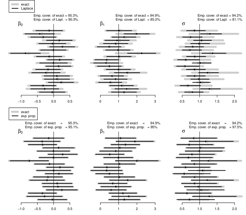
Figure 2: Comparison of point estimation and 95% confidence interval coverage for the first simulation study with true parameter values given by (21). The upper row of panels compares exact maximum likelihood with Laplace approximation. The low row of panels compares exact maximum likelihood with expectation propagation approximation. The horizontal lines indicate expectation propagation-based confidence intervals for 20 randomly chosen replications of the simulation study described in the text. The points indicate the corresponding approximate maximum likelihood estimates. The vertical lines indicate true parameter values. The percentages displayed at the top of each panel are empirical coverages over all $1,000$ replications for each method involved in the comparison.

4.1.2 Accuracy and Speed Assessment for Bivariate Random Effects

In this study we simulated $1,000$ datasets according to a $d^{\mbox{\tiny R}}=2$ version of (1) with true parameter values:

$$\boldsymbol{\beta}_{\mbox{\tiny true}}=[0.37,0.93,-0.46,0.08,-1.34,1.09]^{T}\quad\mbox{and}\quad\boldsymbol{\Sigma}_{\mbox{\tiny true}}=\left[\begin{array}[]{rr}0.53&-0.36\\ -0.36&0.92\end{array}\right].$$ (23)

The number of groups was fixed at $m=250$ and each $n_{i}$ value selected randomly from a discrete Uniform distribution on $\{20,21,\ldots,30\}$. The $\boldsymbol{x}^{\mbox{\tiny F}}_{ij}$ and $\boldsymbol{x}^{\mbox{\tiny R}}_{ij}$ vectors were of the form

$$\boldsymbol{x}^{\mbox{\tiny F}}_{ij}=[1,x_{1,ij},x_{2,ij},x_{3,ij},x_{4,ij},x_{5,ij}]^{T}\quad\mbox{and}\quad\boldsymbol{x}^{\mbox{\tiny R}}_{ij}=[1,x_{1,ij}]^{T}$$

where each $x_{k,ij}$ was generated independently from a Uniform distribution on the unit interval. All relative tolerance values were set to $10^{-5}$ and the maximum number of iteration values were set to $100$, which is relevant for the upcoming speed assessment.

The points and horizontal line segments in Figure 3 are displays of estimates and corresponding 95% confidence intervals for each of the interpretable model parameters, for $50$ randomly chosen replications. The numbers in the top right-hand corner of each panel are the empirical coverage values based on all $1,000$ replications. For all nine parameters, the empirical coverage values are in keeping with the advertized coverage of 95%, and is an indication of excellent accuracy for this setting.

Figure 3: Summary of confidence interval coverage for the second simulation study with true parameter values given by (23). The horizontal lines indicate expectation propagation-based confidence intervals for 50 randomly chosen replications of the simulation study described in the text. The solid circular points indicate the corresponding point estimates. The vertical lines indicate true parameter values. The percentage in the top right-hand corner of each panel is the empirical coverage over all $1,000$ replications.

Despite the higher samples and complexity of the model, we have gotten the fitting times down to tens of seconds in the glmmEP package within the R computing environment. This has been achieved by implementation of Algorithm 1 in a low level language so that approximate likelihood evaluations are very rapid. The computing speed depends upon various relative tolerance values and upper bounds on numbers of iterations for the various iterative schemes as well as attributes of the computer. This simulation study was run on a MacBook Air laptop with 8 gigabytes of random access memory and a 2.2 gigahertz processor. The convergence stopping criteria values are given earlier in this section. Over the 1,000 replications the median computing time was 18 seconds, the upper quartile was 20 seconds and the maximum was 34 seconds. Such speed is impressive given that each data set contained tens of thousands of observations and bivariate random effects are accurately handled.

4.2 Application to Data from a Fertility Study

Data from a 1988 Bangladesh fertility study are stored in the data frame Contraception within the R package mlmRev (Bates, Maechler and Bolker, 2014). Steele, Diamond and Amin (1996) contains details of the study and some multilevel analyses. Variables in the Contraception data frame include:

use

a two-level factor variable indicating whether a woman is a user of contraception at the time of the survey, with levels Y for use and N for non-use,

age

age of the woman in years at the time of the survey, centred about the average age of all women in the study,

district

a multi-level factor variable that codes the district, out of 60 districts in total, in which the woman lives,

urban

a two-level factor variable indicating whether or not the district in which the woman lives is urban, with levels Y for urban dwelling and N for rural dwelling, and

livch

a four-level factor variable that indicates the number of living children of the woman, with levels 0 for no children, 1 for one child, 2 for two children and 3+ for three or more children.

A random intercepts and slopes probit mixed model for these data is

$${\begin{array}[]{rcl}&&I(\texttt{use}_{ij}=\texttt{Y})|u_{0i},u_{1i}\stackrel{{\scriptstyle{\tiny\mbox{ind.}}}}{{\sim}}\mbox{Bernoulli}\Big{(}\Phi\big{(}\beta_{0}+u_{0i}+(\beta_{1}+u_{1i})I(\texttt{urban}_{ij}=\texttt{Y})\\ &&\qquad+\beta_{2}\texttt{age}_{ij}+\beta_{3}\,I(\texttt{livch}_{ij}=\texttt{1})+\beta_{4}\,I(\texttt{livch}_{ij}=\texttt{2})+\beta_{5}\,I(\texttt{livch}_{ij}=\texttt{3+})\big{)}\Big{)}\end{array}}$$ (24)

where $I({\mathcal{P}})=1$ if ${\mathcal{P}}$ is true and $0$ otherwise. Also, $\texttt{use}_{ij}$ denotes the value of use for the $j$th woman within the $i$th district, $1\leq i\leq 60$, with the other variables defined analogously. The bivariate random effects vectors are assumed to satisfy

$$\left[\begin{array}[]{c}u_{0i}\\ u_{1i}\end{array}\right]\stackrel{{\scriptstyle{\tiny\mbox{ind.}}}}{{\sim}}N\left(\left[\begin{array}[]{c}0\\ 0\end{array}\right],\left[\begin{array}[]{cc}\sigma_{1}^{2}&\rho\sigma_{1}\sigma_{2}\\ \rho\sigma_{1}\sigma_{2}&\sigma_{2}^{2}\end{array}\right]\right).$$ (25)

We fitted this model using our expectation propagation approximate likelihood inference scheme. It took about 35 seconds on the fourth author’s MacBook Air laptop (2.2 gigahertz processor and 8 gigabytes of random access memory) to produce the inferential summary given in Table 1.

parameter	95% C.I. low.	estimate	95% C.I. upp.
$\beta_{0}$	$-1.2185$	$-1.0418$	$-0.8651$
$\beta_{1}$	$0.2956$	$0.5003$	$0.7049$
$\beta_{2}$	$-0.0259$	$-0.0164$	$-0.0068$
$\beta_{3}$	$0.4934$	$0.6815$	$0.8698$
$\beta_{4}$	$0.6223$	$0.8306$	$1.0389$
$\beta_{5}$	$0.6102$	$0.8244$	$1.0387$
$\sigma_{1}$	$0.2748$	$0.3785$	$0.5214$
$\sigma_{2}$	$0.3096$	$0.4965$	$0.7962$
$\rho$	$-0.9367$	$-0.7984$	$-0.4446$

Table 1: Expectation propagation approximate maximum likelihood estimates and corresponding 95% confidence interval (C.I.) lower and upper limits for the parameters in model (24) and (25).

Each of the parameters is seen to be statistically significantly different from zero. As examples, the 95% confidence interval for $\beta_{2}$ of $(0.296,0.705)$ indicates a higher use of contraception in urban districts ad the 95% confidence interval for $\sigma_{2}$ of $(0.310,0.796)$ shows that their is signficant heterogeneity in the urban versus rural effect across the 60 districts.

We also used expectation propagation approximate best prediction to obtain predictions of the $u_{0i}$ and $u_{1i}$ values. The results are plotted in Figure 4 and provide a visualization of between-district heterogeneity.

Figure 4: Scatterplot of the expectation propagation-approximate best predictions of the random slopes and corresponding random intercepts for the fit of model given by (24) and (25) to data from a 1998 Bangladesh fertility study.

5 Theoretical Considerations

We now discuss the question regarding whether the excellent inferential accuracy of the Section 3 methodology is supported by theory. A fuller theoretical analysis is the subject of ongoing work involving the first four authors and, upon completion, will be reported elsewhere. In this section we provide a heuristic explanation for the accuracy of expectation propagation in the binary response mixed model context.

First note that the $i$th log-likelihood summand is

$$\ell_{i}(\boldsymbol{\beta},\boldsymbol{\Sigma})=\log\int_{{\mathbb{R}}^{d^{R}}}\left\{\prod_{j=1}^{n_{i}}\frac{p(\boldsymbol{y}_{i}|\boldsymbol{u}_{i};\boldsymbol{\beta})}{{\widetilde{p}}(\boldsymbol{y}_{i}|\boldsymbol{u}_{i};\boldsymbol{\beta})}\right\}\exp\left\{\left[\begin{array}[]{c}1\\ \boldsymbol{u}_{i}\\ \mbox{vech}(\boldsymbol{u}_{i}\boldsymbol{u}_{i}^{T})\end{array}\right]^{T}{\widehat{\underaccent{\sim}{\boldsymbol{\eta}}}}_{i}\right\}\,d\boldsymbol{u}_{i}$$

where ${\widetilde{p}}(\boldsymbol{y}_{i}|\boldsymbol{u}_{i};\boldsymbol{\beta})$ is given by expression (7) with the $\boldsymbol{\eta}_{ij}$ set to the converged $\mbox{\large$\mathbb{\eta}$}_{\mbox{\footnotesize$p(y_{ij}|\boldsymbol{u}_{i};\boldsymbol{\beta})\to\boldsymbol{u}_{i}$}}$ values. We also have

$$\underaccent{\sim}{\ell}_{i}(\boldsymbol{\beta},\boldsymbol{\Sigma})=\log\int_{{\mathbb{R}}^{d^{R}}}\exp\left\{\left[\begin{array}[]{c}1\\ \boldsymbol{u}_{i}\\ \mbox{vech}(\boldsymbol{u}_{i}\boldsymbol{u}_{i}^{T})\end{array}\right]^{T}{\widehat{\underaccent{\sim}{\boldsymbol{\eta}}}}_{i}\right\}\,d\boldsymbol{u}_{i}.$$

Now make the change of variables

$$\boldsymbol{v}=\boldsymbol{\Delta}_{i}^{-1}\{\boldsymbol{u}_{i}-\underaccent{\sim}{\mbox{BP}}(\boldsymbol{u}_{i})\}\quad\mbox{where}\quad\boldsymbol{\Delta}_{i}\equiv\underaccent{\sim}{\mbox{Cov}}(\boldsymbol{u}_{i}|\boldsymbol{y})^{1/2}$$

involving the expectation propagation-approximate best predictor quantities given by (19) and (20). Straightforward manipulations then lead to the discrepancy between $\ell(\boldsymbol{\beta},\boldsymbol{\Sigma})$ and $\underaccent{\sim}{\ell}_{i}(\boldsymbol{\beta},\boldsymbol{\Sigma})$ equalling

$$\ell(\boldsymbol{\beta},\boldsymbol{\Sigma})-\underaccent{\sim}{\ell}_{i}(\boldsymbol{\beta},\boldsymbol{\Sigma})=\log\int_{{\mathbb{R}}^{d^{R}}}\left\{\prod_{j=1}^{n_{i}}A_{ij}(\boldsymbol{\Delta}_{i}\boldsymbol{v})\right\}\phi_{\boldsymbol{I}}(\boldsymbol{v})\,d\boldsymbol{v}$$ (26)

where, for any $\boldsymbol{x}\in{\mathbb{R}}^{d^{\mbox{\tiny R}}}$, $\phi_{I}(\boldsymbol{x})\equiv(2\pi)^{-d^{\mbox{\tiny R}}/2}\exp(-{\textstyle{\frac{1}{2}}}\boldsymbol{x}^{T}\boldsymbol{x})$ and

$$A_{ij}(\boldsymbol{x})\equiv F\Big{(}(2y_{ij}-1)\big{(}\boldsymbol{\beta}^{T}\boldsymbol{x}^{\mbox{\tiny F}}_{ij}+(\underaccent{\sim}{\mbox{BP}}(\boldsymbol{u}_{i})+\boldsymbol{x})^{T}\boldsymbol{x}^{\mbox{\tiny R}}_{ij}\big{)}\Big{)}$$

$$\qquad\qquad\qquad\times\exp\left\{-\left[\begin{array}[]{c}1\\ \underaccent{\sim}{\mbox{BP}}(\boldsymbol{u}_{i})+\boldsymbol{x}\\ \mbox{vech}\Big{(}\big{(}\underaccent{\sim}{\mbox{BP}}(\boldsymbol{u}_{i})+\boldsymbol{x}\big{)}\big{(}\underaccent{\sim}{\mbox{BP}}(\boldsymbol{u}_{i})+\boldsymbol{x}\big{)}^{T}\Big{)}\end{array}\right]^{T}\mbox{\large$\mathbb{\eta}$}_{\mbox{\footnotesize$p(y_{ij}|\boldsymbol{u}_{i};\boldsymbol{\beta})\to\boldsymbol{u}_{i}$}}\right\}.$$

Using the same change of variables, the moment-matching conditions corresponding to the Kullback-Leibler projection (8) are

$$\int_{{\mathbb{R}}^{d^{\mbox{\tiny R}}}}\boldsymbol{v}^{\otimes\,k}A_{ij}(\boldsymbol{\Delta}_{i}\boldsymbol{v})\phi_{I}(\boldsymbol{v})\,d\boldsymbol{v}=\int_{{\mathbb{R}}^{d^{\mbox{\tiny R}}}}\boldsymbol{v}^{\otimes\,k}\phi_{I}(\boldsymbol{v})\,d\boldsymbol{v},\quad k=0,1,2,$$ (28)

where $\boldsymbol{v}^{\otimes\,0}\equiv 1$, $\boldsymbol{v}^{\otimes\,1}\equiv\boldsymbol{v}$ and $\boldsymbol{v}^{\otimes\,2}=\boldsymbol{v}\boldsymbol{v}^{T}$.

To aid intuition, for the remainder of this section we restrict attention to $d^{\mbox{\tiny R}}=1$ and write $\delta_{i}$ instead of $\boldsymbol{\Delta}_{i}$ to signify the fact that this quantity is scalar in this special case. Next, we make the

$$\mbox{working assumption:}\quad\delta_{i}=O_{p}(n_{i}^{-1/2}).$$ (29)

This assumption is in keeping with the fact that $\delta_{i}$ is the expectation propagation approximation to the sample standard deviation of $\underaccent{\sim}{\mbox{BP}}(\boldsymbol{u}_{i})-\boldsymbol{u}_{i}$. Then Taylor series expansion of $A_{ij}$ about zero and substitution into the $d^{\mbox{\tiny R}}=1$ version of (28) leads to

$$A_{ij}(0)=1+O(\delta_{i}^{4}),\quad A^{\prime}_{ij}(0)=O(\delta_{i}^{2})\quad\mbox{and}\quad A^{\prime\prime}_{ij}(0)=O(\delta_{i}^{2}).$$

Plugging these into (26) and using $\log(1+\varepsilon)\approx\varepsilon$ for small $\varepsilon$ we obtain

$$\ell_{i}(\boldsymbol{\beta},\boldsymbol{\Sigma})-\underaccent{\sim}{\ell}_{i}(\boldsymbol{\beta},\boldsymbol{\Sigma})=O_{p}(n_{i}^{-1/2})\quad\mbox{under}\ (\ref{eq:workAss}).$$

These heuristics suggest that expectation propagation provides consistent estimation of the log-likelihood summands as the number of measurements in the $i$th group increases. The deeper question concerning the asymptotic statistical properties of the expectation propagation-based estimators (${\widehat{\underaccent{\sim}{\boldsymbol{\beta}}}},{\widehat{\underaccent{\sim}{\boldsymbol{\Sigma}}}})$ requires more delicate theoretical analysis. As mentioned earlier in this section, this question is being pursued by authors of this article.

Before closing this section, we mention that there is a small but emerging body of research concerning the large sample behavior of expectation propagation for approximation Bayesian inference. A recent contribution of this type is Dehaene & Barthelmé (2018) which provides Bernstein-von Mises theory for Bayesian expectation propagation.

6 Higher Level and Crossed Random Effects Extensions

The binary mixed model given by (1) is adequate for the common situation of there being only one grouping mechanism. However, more elaborate models are required for situations such as hierarchical and cross-tabulated grouping mechanisms. Goldstein (2010), for example, provides an extensive treatment of mixed models with higher levels of nesting. A major reference for crossed random effects mixed models is Baayen, Davidson & Bates (2008). Here we provide advice regarding extension our expectation propagation approach to these settings.

The two levels of nesting extension of (1) is

$$\begin{array}[]{c}y_{ijk}|\boldsymbol{u}^{\mbox{\tiny L1}}_{i},\boldsymbol{u}^{\mbox{\tiny L2}}_{ij}\stackrel{{\scriptstyle{\tiny\mbox{ind.}}}}{{\sim}}\mbox{Bernoulli}\Big{(}F\big{(}\boldsymbol{\beta}^{T}\boldsymbol{x}^{\mbox{\tiny F}}_{ijk}+(\boldsymbol{u}^{\mbox{\tiny L1}}_{i})^{T}\boldsymbol{x}^{\mbox{\tiny R1}}_{ijk}+(\boldsymbol{u}^{\mbox{\tiny L2}}_{ij})^{T}\boldsymbol{x}^{\mbox{\tiny R2}}_{ijk}\big{)}\Big{)},\\[8.61108pt] \boldsymbol{u}^{\mbox{\tiny L1}}_{i}\stackrel{{\scriptstyle{\tiny\mbox{ind.}}}}{{\sim}}N(\boldsymbol{0},\boldsymbol{\Sigma}^{\mbox{\tiny L1}})\ \mbox{independently of}\ \boldsymbol{u}^{\mbox{\tiny L2}}_{ij}\stackrel{{\scriptstyle{\tiny\mbox{ind.}}}}{{\sim}}N(\boldsymbol{0},\boldsymbol{\Sigma}^{\mbox{\tiny L2}}),\\[8.61108pt] 1\leq i\leq m,\quad 1\leq j\leq n_{i},\quad 1\leq k\leq o_{ij}.\end{array}$$ (30)

The response $y_{ijk}$ and predictor vectors $\boldsymbol{x}^{\mbox{\tiny F}}_{ijk}$, $\boldsymbol{x}^{\mbox{\tiny R1}}_{ijk}$ and $\boldsymbol{x}^{\mbox{\tiny R2}}_{ijk}$ correspond to the $k$th set of measurements within the $j$th inner group within the $i$th outer group. The number of outer groups is $m$ and the number of inner groups in the $i$th outer group is $n_{i}$. The sample size of the $j$th group in the $i$th outer group is $o_{ij}$. Also, $\boldsymbol{x}^{\mbox{\tiny R1}}_{ijk}$ is $d^{\mbox{\tiny R1}}\times 1$ and $\boldsymbol{x}^{\mbox{\tiny R2}}_{ijk}$ is $d^{\mbox{\tiny R2}}\times 1$. The log-likelihood of $(\boldsymbol{\beta},\boldsymbol{\Sigma}^{\mbox{\tiny L1}},\boldsymbol{\Sigma}^{\mbox{\tiny L2}})$ may be written as

$$\ell(\boldsymbol{\beta},\boldsymbol{\Sigma}^{\mbox{\tiny L1}},\boldsymbol{\Sigma}^{\mbox{\tiny L2}})=\sum_{i=1}^{m}\log\int_{{\mathbb{R}}^{d^{\mbox{\tiny R}}}}\prod_{j=1}^{n_{i}}\prod_{k=1}^{o_{ij}}p\left(y_{ijk}\Bigg{|}\left[\begin{array}[]{c}\boldsymbol{u}^{\mbox{\tiny L1}}_{i}\\ \boldsymbol{u}^{\mbox{\tiny L2}}_{ij}\end{array}\right];\boldsymbol{\beta}\right)p\left(\left[\begin{array}[]{c}\boldsymbol{u}^{\mbox{\tiny L1}}_{i}\\ \boldsymbol{u}^{\mbox{\tiny L2}}_{ij}\end{array}\right];\boldsymbol{\Sigma}^{\mbox{\tiny L1}},\boldsymbol{\Sigma}^{\mbox{\tiny L2}}\right)\,d\left[\begin{array}[]{c}\boldsymbol{u}^{\mbox{\tiny L1}}_{i}\\ \boldsymbol{u}^{\mbox{\tiny L2}}_{ij}\end{array}\right]$$ (31)

where $d^{\mbox{\tiny R}}=d^{\mbox{\tiny R1}}+d^{\mbox{\tiny R2}}$,

$$p\left(y_{ijk}\Bigg{|}\left[\begin{array}[]{c}\boldsymbol{u}^{\mbox{\tiny L1}}_{i}\\ \boldsymbol{u}^{\mbox{\tiny L2}}_{ij}\end{array}\right];\boldsymbol{\beta}\right)\equiv F\Big{(}(2y_{ijk}-1)\big{(}\boldsymbol{\beta}^{T}\boldsymbol{x}^{\mbox{\tiny F}}_{ijk}+(\boldsymbol{u}^{\mbox{\tiny L1}}_{i})^{T}\boldsymbol{x}^{\mbox{\tiny R1}}_{ijk}+(\boldsymbol{u}^{\mbox{\tiny L2}}_{ij})^{T}\boldsymbol{x}^{\mbox{\tiny R2}}_{ijk}\big{)}\Big{)},\ y_{ijk}=0,1,$$

and

$$p\left(\left[\begin{array}[]{c}\boldsymbol{u}^{\mbox{\tiny L1}}_{i}\\ \boldsymbol{u}^{\mbox{\tiny L2}}_{ij}\end{array}\right];\boldsymbol{\Sigma}^{\mbox{\tiny L1}},\boldsymbol{\Sigma}^{\mbox{\tiny L2}}\right)\equiv|2\pi\boldsymbol{\Sigma}^{\mbox{\tiny L1}}|^{-1/2}|2\pi\boldsymbol{\Sigma}^{\mbox{\tiny L2}}|^{-1/2}\exp\left\{-{\textstyle{\frac{1}{2}}}\left[\begin{array}[]{c}\boldsymbol{u}^{\mbox{\tiny L1}}_{i}\\ \boldsymbol{u}^{\mbox{\tiny L2}}_{ij}\end{array}\right]^{T}\left[\begin{array}[]{cc}\boldsymbol{\Sigma}^{\mbox{\tiny L1}}&\boldsymbol{0}\\ \boldsymbol{0}&\boldsymbol{\Sigma}^{\mbox{\tiny L2}}\end{array}\right]^{-1}\left[\begin{array}[]{c}\boldsymbol{u}^{\mbox{\tiny L1}}_{i}\\ \boldsymbol{u}^{\mbox{\tiny L2}}_{ij}\end{array}\right]\right\}.$$

Expectation propagation approximation of $\ell(\boldsymbol{\beta},\boldsymbol{\Sigma}^{\mbox{\tiny L1}},\boldsymbol{\Sigma}^{\mbox{\tiny L2}})$ then proceeds by message passing on the factor graph displayed in Figure 5. In the probit case Theorem 1 can be called upon to obtain closed form updates for the message natural parameter vectors leading to an algorithm analogous to Algorithm 1.

Figure 5: Factor graph representation of the product structure of the integrand in (6). The open circle corresponds to the random effect vector $[\boldsymbol{u}^{\mbox{\tiny L1}}_{i}\ \boldsymbol{u}^{\mbox{\tiny L2}}_{ij}]^{T}$ and the solid rectangles indicate factors in the integrand of (31). Edges indicate dependence of each factor on $[\boldsymbol{u}^{\mbox{\tiny L1}}_{i}\ \boldsymbol{u}^{\mbox{\tiny L2}}_{ij}]^{T}$.

A crossed random effects extension of (1) is

$$\begin{array}[]{c}y_{ii^{\prime}j}|\boldsymbol{u}_{i},\boldsymbol{u}^{\prime}_{i^{\prime}}\stackrel{{\scriptstyle{\tiny\mbox{ind.}}}}{{\sim}}\mbox{Bernoulli}\Big{(}F\big{(}\boldsymbol{\beta}^{T}\boldsymbol{x}^{\mbox{\tiny F}}_{ii^{\prime}j}+(\boldsymbol{u}_{i})^{T}\boldsymbol{x}^{\mbox{\tiny R}}_{ii^{\prime}j}+(\boldsymbol{u}^{\prime}_{i^{\prime}})^{T}\boldsymbol{x}^{\mbox{\tiny R$\prime$}}_{ii^{\prime}j}\big{)}\Big{)},\\[8.61108pt] \boldsymbol{u}_{i}\stackrel{{\scriptstyle{\tiny\mbox{ind.}}}}{{\sim}}N(\boldsymbol{0},\boldsymbol{\Sigma})\ \mbox{independently of}\ \boldsymbol{u}^{\prime}_{i^{\prime}}\stackrel{{\scriptstyle{\tiny\mbox{ind.}}}}{{\sim}}N(\boldsymbol{0},\boldsymbol{\Sigma}^{\prime}),\\[8.61108pt] 1\leq i\leq m,\quad 1\leq i^{\prime}\leq m^{\prime},\quad 1\leq j\leq n_{ii^{\prime}}\end{array}$$

where the data are cross-tabulated according to membership of two groups of sizes $m$ and $m^{\prime}$ indexed according to the pair $(i,i^{\prime})\in\{1,\ldots,m\}\times\{1,\ldots,m^{\prime}\}$, with $n_{ii^{\prime}}$ denoting the sample size within group $(i,i^{\prime})$. Note that $n_{ii^{\prime}}=0$ is a possibility for some $(i,i^{\prime})$. The response $y_{ii^{\prime}j}$ and the predictor vectors $\boldsymbol{x}^{\mbox{\tiny F}}_{ii^{\prime}j}$, $\boldsymbol{x}^{\mbox{\tiny R}}_{ii^{\prime}j}$ and $\boldsymbol{x}^{\mbox{\tiny R$\prime$}}_{ii^{\prime}j}$ correspond to the $j$th set of measurements within group $(i,i^{\prime})$. The $\boldsymbol{u}_{i}$, $1\leq i\leq m$, are $d^{\mbox{\tiny R}}\times 1$ random effects for group-specific departures from the fixed effects for the first group. The $\boldsymbol{u}^{\prime}_{i}$, $1\leq i\leq m^{\prime}$, are $d^{\mbox{\tiny R$\prime$}}\times 1$ random effects for group-specific departures from the fixed effects for the second group. The log-likelihood of $(\boldsymbol{\beta},\boldsymbol{\Sigma},\boldsymbol{\Sigma}^{\prime})$ is

$$\ell(\boldsymbol{\beta},\boldsymbol{\Sigma},\boldsymbol{\Sigma}^{\prime})=\sum_{i=1}^{m}\sum_{i^{\prime}=1}^{m^{\prime}}I(n_{ii^{\prime}}>0)\log\int_{{\mathbb{R}}^{d^{\mbox{\tiny R}}+d^{\mbox{\tiny R$\prime$}}}}\prod_{j=1}^{n_{ii^{\prime}}}p\left(y_{ii^{\prime}j}\Bigg{|}\left[\begin{array}[]{c}\boldsymbol{u}_{i}\\ \boldsymbol{u}^{\prime}_{i^{\prime}}\end{array}\right];\boldsymbol{\beta}\right)p\left(\left[\begin{array}[]{c}\boldsymbol{u}_{i}\\ \boldsymbol{u}^{\prime}_{i^{\prime}}\end{array}\right];\boldsymbol{\Sigma},\boldsymbol{\Sigma}^{\prime}\right)\,d\left[\begin{array}[]{c}\boldsymbol{u}_{i}\\ \boldsymbol{u}^{\prime}_{i^{\prime}}\end{array}\right]$$

where

$$p\left(y_{ii^{\prime}j}\Bigg{|}\left[\begin{array}[]{c}\boldsymbol{u}_{i}\\ \boldsymbol{u}^{\prime}_{i^{\prime}}\end{array}\right];\boldsymbol{\beta}\right)\equiv F\Big{(}(2y_{ijk}-1)\big{(}\boldsymbol{\beta}^{T}\boldsymbol{x}^{\mbox{\tiny F}}_{ii^{\prime}j}+(\boldsymbol{u}_{i})^{T}\boldsymbol{x}^{\mbox{\tiny R}}_{ii^{\prime}j}+(\boldsymbol{u}^{\prime}_{i^{\prime}})^{T}\boldsymbol{x}^{\mbox{\tiny R$\prime$}}_{ii^{\prime}j}\big{)}\Big{)},\ y_{ijk}=0,1,$$

and

$$p\left(\left[\begin{array}[]{c}\boldsymbol{u}_{i}\\ \boldsymbol{u}^{\prime}_{i^{\prime}}\end{array}\right];\boldsymbol{\Sigma},\boldsymbol{\Sigma}^{\prime}\right)\equiv|2\pi\boldsymbol{\Sigma}|^{-1/2}|2\pi\boldsymbol{\Sigma}^{\prime}|^{-1/2}\exp\left\{-{\textstyle{\frac{1}{2}}}\left[\begin{array}[]{c}\boldsymbol{u}_{i}\\ \boldsymbol{u}^{\prime}_{i^{\prime}}\end{array}\right]^{T}\left[\begin{array}[]{cc}\boldsymbol{\Sigma}&\boldsymbol{0}\\ \boldsymbol{0}&\boldsymbol{\Sigma}^{\prime}\end{array}\right]^{-1}\left[\begin{array}[]{c}\boldsymbol{u}_{i}\\ \boldsymbol{u}^{\prime}_{i^{\prime}}\end{array}\right]\right\}.$$

Expectation propagation approximation of $\ell(\boldsymbol{\beta},\boldsymbol{\Sigma},\boldsymbol{\Sigma}^{\prime})$ can be achieved via message passing on a factor graph similar to that shown in Figure 5.

7 Transferral to Other Mixed Models

Until now we have mainly focused on the special case of probit mixed models with Gaussian random effects since the requisite Kullback-Leibler projections have closed form solutions. However, our approach is quite general and, at least in theory, applies to other mixed models. We now briefly describe transferral to other mixed models.

7.1 Logistic Mixed Models

As we mention in Section 2, the probit and logistic cases are distinguished according to whether $F=\Phi$ or $F=\mbox{expit}$. Therefore, transferral from probit to logistic mixed models involves replacement of $f_{\mbox{\tiny input}}$ in Theorem 1 by

$$f_{\mbox{\tiny input}}(\boldsymbol{x})=\mbox{expit}(c_{0}+\boldsymbol{c}_{1}^{T}\boldsymbol{x})\exp\left\{\left[\begin{array}[]{c}\boldsymbol{x}\\ \mbox{vech}(\boldsymbol{x}\boldsymbol{x}^{T})\end{array}\right]^{T}\left[\begin{array}[]{c}\boldsymbol{\eta}_{1}^{\mbox{\tiny{input}}}\\[4.30554pt] \boldsymbol{\eta}_{2}^{\mbox{\tiny{input}}}\end{array}\right]\right\},\quad\boldsymbol{x}\in{\mathbb{R}}^{d}.$$ (32)

In view of Lemma 1 of the online supplement, Kullback-Leibler projection of $f_{\mbox{\tiny input}}$ onto the unnormalized Normal family involves univariate integrals of the form

$$\int_{-\infty}^{\infty}\,x^{p}\exp\{qx-rx^{2}-\log(1+e^{x})\}\,dx,\quad p=0,1,2,\ q\in{\mathbb{R}},\ r>0.$$ (33)

In the Bayesian context, Gelman et al. (2014; Section 13.8) and Kim & Wand (2017) describe quadrature-based approaches to evaluation of (33), each of which transfers to the frequentist context dealt with here. However, there is a significant speed cost compared with the probit case.

An alternative approach involves use of the family of approximations to expit of the form

$$\mbox{expit}_{k}(x)\equiv\sum_{i=1}^{k}\,p_{k,i}\Phi(s_{k,i}x)$$

for constants $p_{k,i}$ and $s_{k,i}$, as advocated by Monahan & Stefanski (1989). Since the approximation is a linear combination of scalings of $\Phi$, the function $f_{\mbox{\tiny input}}$ in (32) with expit replaced by $\mbox{expit}_{k}$ admits closed form Kullback-Leibler projections onto the unnormalized Multivariate Normal, leading to fast and accurate inference for logistic mixed models.

Details on the mechanics and performance of expectation propagation for logistic mixed models is to be reported in Yu (2019).

7.2 Other Generalized Linear Mixed Models

Whilst we have focused on the binary response situation in this article, we quickly point out that the principles apply to other generalized linear mixed models such as those based on the Gamma and Poisson families. Note that (2) with $F=\mbox{expit}$ generalizes to

$$\ell(\boldsymbol{\beta},\boldsymbol{\Sigma})=\sum_{i=1}^{m}\log\int_{d^{\mbox{\tiny R}}}\left[\prod_{j=1}^{n_{i}}\exp\Big{\{}y_{ij}(\boldsymbol{\beta}^{T}\boldsymbol{x}^{\mbox{\tiny F}}_{ij}+\boldsymbol{u}^{T}\boldsymbol{x}^{\mbox{\tiny R}}_{ij})-b\big{(}\boldsymbol{\beta}^{T}\boldsymbol{x}^{\mbox{\tiny F}}_{ij}+\boldsymbol{u}^{T}\boldsymbol{x}^{\mbox{\tiny R}}_{ij}\big{)}+c(y_{ij})\Big{\}}\right]$$

$$\qquad\qquad\times|2\pi\boldsymbol{\Sigma}|^{-1/2}\exp(-{\textstyle{\frac{1}{2}}}\boldsymbol{u}^{T}\boldsymbol{\Sigma}^{-1}\boldsymbol{u})\,d\boldsymbol{u}$$

where the functions $b$ and $c$ are as given in Table 2.1 of McCullagh & Nelder (1989). Setting $b(x)=\log(1+e^{x})$ and $c(x)=0$ gives the $F=\mbox{expit}$ logistic mixed model while putting $b(x)=e^{x}$ and $c(x)=-\log(x!)$ gives the corresponding Poisson mixed model. The family of integrals

$$\int_{-\infty}^{\infty}\,x^{p}\exp\{qx-rx^{2}-b(x)\}\,dx,\quad p=0,1,2,\ q\in{\mathbb{R}},\ r>0,$$

is required to facilitate the required Kullback-Leibler projections for the $d^{\mbox{\tiny R}}=1$ case. With the exception of logistic mixed models, multivariate numerical integration appears to be required when $d^{\mbox{\tiny R}}>1$. Yu (2019) will contain a detailed account of the practicalities and performance of expectation propagation for this class of models.

References

Azzalini, A. (2017). The R package sn: The skew-normal and skew-t distributions (version 1.5). http://azzalini.stat.unipd.it/SN

Baayen, R.H., Davidson, D.J. and Bates, D.M. (2008). Mixed-effects modeling with crossed random effects for subjects and items. Journal of Memory and Language, 59, 390–412.

Bates, D., Maechler, M. and Bolker, B. (2014). mlmRev: Examples from multilevel modelling software review. R package version 1.0.
http://cran.r-project.org.

Baltagi, B.H. (2013). Econometric Analysis of Panel Data, Fifth Edition. Chichester, U.K.: John Wiley & Sons.

Bates, D., Maechler, M., Bolker, B. and Walker, S. (2015). Fitting linear mixed-effects models using lme4. Journal of Statistical Software, 67(1), 1–48.

Bishop, C.M. (2006). Pattern Recognition and Machine Learning. New York: Springer.

Broyden, C.G. (1970). The convergence of a class of double-rank minimization algorithms. Journal of the Institute of Mathematics and Its Applications, 6, 76–90.

Carlin, B.P. and Gelfand, A.E. (1991). A sample reuse method for accurate parametric empirical Bayes confidence intervals. Journal of the Royal Statistical Society, Series B, 53, 189–200.

Dehaene, G. and Barthelmé, S. (2018). Expectation propagation in the large-data limit. Journal of the Royal Statistical Society, Series B, 80, 199–217.

Diggle, P., Heagerty, P., Liang, K.-L. and Zeger, S. (2002). Analysis of Longitudinal Data, Second Edition. Oxford, U.K.: Oxford University Press.

Fletcher, R. (1970). A new approach to variable metric algorithms. Computer Journal, 13, 317–322.

Gelman, A., Carlin, J.B., Stern, H.S., Dunson, D.B.,Vehtari, A. and Rubin, D.B. (2014). Bayesian Data Analysis, Third Edition, Boca Raton, Florida: CRC Press.

Gelman, A. and Hill, J. (2007). Data Analysis using Regression and Multilevel/Hierarchical Models. New York: Cambridge University Press.

Givens, G.H. and Hoetig, J.A. (2005). Computational Statistics, Hoboken, New Jersey: John Wiley & Sons.

Goldfarb, D. (1970). A family of variable metric updates derived by variational means. Mathematics of Computation, 24, 23–26.

Goldstein, H. (2010). Multilevel Statistical Models, Fourth Edition. Chichester, U.K.: John Wiley & Sons.

Harville, D.A. (2008). Matrix Algebra from a Statistician’s Perspective. New York: Springer.

Kim, A.S.I. and Wand, M.P. (2017). On expectation propagation for generalised, linear and mixed models. Australian and New Zealand Journal of Statistics, 59, in press.

Magnus, J.R. and Neudecker, H. (1999). Matrix Differential Calculus with Applications in Statistics and Econometrics, Revised Edition. Chichester U.K.: Wiley.

Mardia, K.V., Kent, J.T. and Bibby, J.M. (1979). Multivariate Analysis. London: Academic Press.

The Mathworks Incorporated (2018). Natick, Massachusetts, U.S.A.

McCullagh, P. and Nelder, J.A. (1989). Generalized Linear Models, Second Edition. London: Chapman and Hall.

McCulloch, C.E., Searle, S.R. and Neuhaus, J.M. (2008). Generalized, Linear, and Mixed Models, Second Edition. New York: John Wiley & Sons.

Minka, T.P. (2001). Expectation propagation for approximate Bayesian inference. In J.S. Breese & D. Koller (eds), Proceedings of the Seventeenth Conference on Uncertainty in Artificial Intelligence, pp. 362–369. Burlington, Massachusetts: Morgan Kaufmann.

Minka, T. (2005). Divergence measures and message passing. Microsoft Research Technical Report Series, MSR-TR-2005-173, 1–17.

Minka, T. & Winn, J. (2008), Gates: A graphical notation for mixture models. Microsoft Research Technical Report Series, MSR-TR-2008-185, 1–16.

Monahan, J.F. & Stefanski, L.A. (1989). Normal scale mixture approximations to $F^{*}(z)$ and computation of the logistic-normal integral. In Balakrishnan, N. (editor), Handbook of the Logistic Distribution. New York: Marcel Dekker, 529–540.

Nelder, J.A. and Mead, R. (1965). A simplex method for function minimization. Computer Journal, 7, 308–313.

Pinheiro, J.C. and Bates, D.M. (2000). Mixed-Effects Models in S and S-PLUS. New York: Springer.

R Core Team (2018). R: A language and environment for statistical computing. R Foundation for Statistical Computing, Vienna, Austria. https://www.R-project.org/.

Rao, J.N.K. and Molina, I. (2015). Small Area Estimation, Second Edition. Hoboken, New Jersey: John Wiley & Sons.

Rue, H., Martino, S. and Chopin, N. (2009). Approximate Bayesian inference for latent Gaussian models by using integrated nested Laplace approximations (with discussion). Journal of the Royal Statistical Society, Series B, 71, 319–392.

Shanno, D.F. (1970). Conditioning of quasi-Newton methods for function minimization. Mathematics of Computation, 24, 647–656.

Steele, F., Diamond, I. and Amin, S. (1996). Immunization uptake in rural Bangladesh: a multilevel analysis. Journal of the Royal Statistical Society, Series A, 159, 289–299.

The Mathworks Incorporated (2018). Natick, Massachusetts, U.S.A.

Wainwright, M.J. and Jordan, M.I. (2008). Graphical models, exponential families, and variational inference. Foundations and Trends in Machine Learning, 1, 1–305.

Wand, M.P. and Ormerod, J.T. (2012). Continued fraction enhancement of Bayesian computing. Stat, 1, 31–41.

Wand, M.P. and Yu, J.C.F. (2018). glmmEP: Fast and accurate likelihood-based inference in generalized linear mixed models via expectation propagation. R package version 0.999. http://cran.r-project.org.

Yu, J.C.F. (2019). Fast and Accurate Frequentist Generalized Linear Mixed Model Analysis via Expectation Propagation. Doctor of Philosophy thesis, University of Technology Sydney.

Supplement for:

Fast and Accurate Binary Response Mixed Model

Analysis via Expectation Propagation

By P. Hall¹, I.M. Johnstone², J.T. Ormerod³, M.P. Wand⁴ and J.C.F. Yu⁴

¹University of Melbourne, ²Stanford University, ³University of Sydney

and ⁴University of Technology Sydney

S.1 Proof of Theorem 1

For $\boldsymbol{x}\in{\mathbb{R}}^{d}$, define

$$\phi_{\boldsymbol{\Sigma}}(\boldsymbol{x})\equiv(2\pi)^{-d/2}|\boldsymbol{\Sigma}|^{-1/2}\exp\big{(}-{\textstyle{\frac{1}{2}}}\boldsymbol{x}^{T}\boldsymbol{\Sigma}^{-1}\boldsymbol{x}\big{)}$$

so that

$$\phi_{\boldsymbol{I}}(\boldsymbol{x})=(2\pi)^{-d/2}\exp\big{(}-{\textstyle{\frac{1}{2}}}\boldsymbol{x}^{T}\boldsymbol{x}\big{)}.$$

We continue to use an unadorned $\phi$ to denote the Univariate Normal density function:

$$\phi(x)=(2\pi)^{-1/2}\exp(-{\textstyle{\frac{1}{2}}}\,x^{2}).$$

The notation $\|\boldsymbol{v}\|=\sqrt{\boldsymbol{v}^{T}\boldsymbol{v}}$ for a column vector $\boldsymbol{v}$ is also used.

Lemma 1. For any function $g:{\mathbb{R}}\to{\mathbb{R}}$ and $d\times 1$ vectors $\boldsymbol{\alpha}_{1}$, $\boldsymbol{\alpha}_{2}$ and $\boldsymbol{\alpha}_{3}$ such that the integrals exist:

$$\int_{{\mathbb{R}}^{d}}g(\boldsymbol{\alpha}_{1}^{T}\boldsymbol{x})\phi_{\boldsymbol{I}}(\boldsymbol{x})\,d\boldsymbol{x} = \int_{-\infty}^{\infty}g(\|\boldsymbol{\alpha}_{1}\|\,z)\phi(z)\,dz,$$ (S.1)

$$\int_{{\mathbb{R}}^{d}}g(\boldsymbol{\alpha}_{1}^{T}\boldsymbol{x})(\boldsymbol{\alpha}_{2}^{T}\boldsymbol{x})\phi_{\boldsymbol{I}}(\boldsymbol{x})\,d\boldsymbol{x} = \{(\boldsymbol{\alpha}_{1}^{T}\boldsymbol{\alpha}_{2})/\|\boldsymbol{\alpha}_{1}\|\}\int_{-\infty}^{\infty}z\,g(\|\boldsymbol{\alpha}_{1}\|\,z)\phi(z)\,dz$$ (S.2)

$$\textit{and}\ \int_{{\mathbb{R}}^{d}}g(\boldsymbol{\alpha}_{1}^{T}\boldsymbol{x})(\boldsymbol{\alpha}_{2}^{T}\boldsymbol{x})(\boldsymbol{\alpha}_{3}^{T}\boldsymbol{x})\phi_{\boldsymbol{I}}(\boldsymbol{x})\,d\boldsymbol{x} = (\boldsymbol{\alpha}_{2}^{T}\boldsymbol{\alpha}_{3})\int_{-\infty}^{\infty}g(\|\boldsymbol{\alpha}_{1}\|\,z)\phi(z)\,dz$$

$$\hskip-85.35826pt+\{(\boldsymbol{\alpha}_{1}^{T}\boldsymbol{\alpha}_{2})(\boldsymbol{\alpha}_{1}^{T}\boldsymbol{\alpha}_{3})/\|\boldsymbol{\alpha}_{1}\|^{2}\}\int_{-\infty}^{\infty}(z^{2}-1)g(\|\boldsymbol{\alpha}_{1}\|\,z)\phi(z)\,dz.$$

Proof of Lemma 1. Lemma 1 is a consequence of the fact that the integrals on the left-hand side are, respectively,

$$E\{g(\boldsymbol{\alpha}_{1}^{T}\boldsymbol{x})\},\ E\{g(\boldsymbol{\alpha}_{1}^{T}\boldsymbol{x})(\boldsymbol{\alpha}_{2}^{T}\boldsymbol{x})\}\quad\mbox{and}\quad E\{g(\boldsymbol{\alpha}_{1}^{T}\boldsymbol{x})(\boldsymbol{\alpha}_{2}^{T}\boldsymbol{x})(\boldsymbol{\alpha}_{3}^{T}\boldsymbol{x})\}$$

where

$$\boldsymbol{x}\sim\mbox{N}(\boldsymbol{0}_{d},\boldsymbol{I}_{d}).$$

We now focus on simplification of the third integral (S.1). Simplication of the first and second integrals is similar and simpler. Make the change of variables

$$\boldsymbol{s}\equiv\left[\begin{array}[]{c}s_{1}\\ s_{2}\\ s_{3}\end{array}\right]=\boldsymbol{A}\boldsymbol{x}\quad\mbox{where}\quad\boldsymbol{A}\equiv\left[\begin{array}[]{c}\boldsymbol{\alpha}_{1}^{T}\\ \boldsymbol{\alpha}_{2}^{T}\\ \boldsymbol{\alpha}_{3}^{T}\end{array}\right]$$

so that

$$E\{g(\boldsymbol{\alpha}_{1}^{T}\boldsymbol{x})(\boldsymbol{\alpha}_{2}^{T}\boldsymbol{x})(\boldsymbol{\alpha}_{3}^{T}\boldsymbol{x})\}=E\{g(s_{1})s_{2}s_{3}\}\quad\mbox{where}\quad\boldsymbol{s}\sim N(\boldsymbol{0}_{3},\boldsymbol{A}\boldsymbol{A}^{T}).$$

We then note that,

$$E\{g(s_{1})s_{2}s_{3}\} = \int_{-\infty}^{\infty}g(s_{1})\left\{\int_{-\infty}^{\infty}\int_{-\infty}^{\infty}s_{2}s_{3}p(s_{2}s_{3}|s_{1})ds_{2}ds_{3}\right\}p(s_{1})ds_{1}$$

$$= \int_{-\infty}^{\infty}g(s_{1})\left\{\int_{-\infty}^{\infty}\int_{-\infty}^{\infty}\{\mbox{Cov}(s_{2},s_{3}|s_{1})+E(s_{2}|s_{1})E(s_{3}|s_{1})\}ds_{2}ds_{3}\right\}p(s_{1})ds_{1}$$

and make use of the result (see e.g. Theorem 3.2.4 of Mardia, Kent & Bibby, 1979)

$$\left[\begin{array}[]{c}s_{2}\\[4.30554pt] s_{3}\end{array}\right]\Bigg{|}s_{1}\sim N\Bigg{(}(s_{1}/\|\boldsymbol{\alpha}_{1}\|^{2})\left[\begin{array}[]{c}\boldsymbol{\alpha}_{1}^{T}\boldsymbol{\alpha}_{2}\\[4.30554pt] \boldsymbol{\alpha}_{1}^{T}\boldsymbol{\alpha}_{3}\end{array}\right],$$

$$\quad\qquad\qquad\qquad\left[\begin{array}[]{ccc}\|\boldsymbol{\alpha}_{2}\|^{2}&&\boldsymbol{\alpha}_{2}^{T}\boldsymbol{\alpha}_{3}\\[4.30554pt] \boldsymbol{\alpha}_{2}^{T}\boldsymbol{\alpha}_{3}&&\|\boldsymbol{\alpha}_{3}\|^{2}\end{array}\right]-(1/\|\boldsymbol{\alpha}_{1}\|^{2})\left[\begin{array}[]{ccc}(\boldsymbol{\alpha}_{1}^{T}\boldsymbol{\alpha}_{2})^{2}&&(\boldsymbol{\alpha}_{1}^{T}\boldsymbol{\alpha}_{2})(\boldsymbol{\alpha}_{1}^{T}\boldsymbol{\alpha}_{3})\\[4.30554pt] (\boldsymbol{\alpha}_{1}^{T}\boldsymbol{\alpha}_{2})(\boldsymbol{\alpha}_{1}^{T}\boldsymbol{\alpha}_{3})&&(\boldsymbol{\alpha}_{1}^{T}\boldsymbol{\alpha}_{3})^{2}\end{array}\right]\Bigg{)}.$$

Result (S.1) then follows via simple algebraic manipulations.

Lemma 2. For all $a\in{\mathbb{R}}$ and $d\times 1$ vectors $\boldsymbol{b}$

$$\int_{{\mathbb{R}}^{d}}\Phi(a+\boldsymbol{b}^{T}\boldsymbol{x})\phi_{\boldsymbol{I}}(\boldsymbol{x})\,dx = \Phi\left(\frac{a}{\sqrt{\boldsymbol{b}^{T}\boldsymbol{b}+1}}\right),$$ (S.6)

$$\int_{{\mathbb{R}}^{d}}\,\boldsymbol{x}\,\Phi(a+\boldsymbol{b}^{T}\boldsymbol{x})\phi_{\boldsymbol{I}}(\boldsymbol{x})\,dx = \frac{\boldsymbol{b}}{\sqrt{\boldsymbol{b}^{T}\boldsymbol{b}+1}}\,\phi\left(\frac{a}{\sqrt{\boldsymbol{b}^{T}\boldsymbol{b}+1}}\right)\quad\mbox{{and}}$$ (S.7)

$$\int_{{\mathbb{R}}^{d}}\,\boldsymbol{x}\boldsymbol{x}^{T}\,\Phi(a+\boldsymbol{b}^{T}\boldsymbol{x})\phi_{I}(\boldsymbol{x})\,dx = \Phi\left(\frac{a}{\sqrt{\boldsymbol{b}^{T}\boldsymbol{b}+1}}\right)\!\boldsymbol{I}-\!\frac{a\boldsymbol{b}\boldsymbol{b}^{T}}{\sqrt{(\boldsymbol{b}^{T}\boldsymbol{b}+1)^{3}}}\phi\left(\frac{a}{\sqrt{\boldsymbol{b}^{T}\boldsymbol{b}+1}}\right).$$ (S.8)

Proof of Lemma 2.

Suppose that $Z_{1}$ and $Z_{2}$ are independent $N(0,1)$ random variables. As defined in Section 4.2, for a logical proposition ${\mathcal{P}}$, let $I({\mathcal{P}})=1$ if ${\mathcal{P}}$ is true and $I({\mathcal{P}})=0$ if ${\mathcal{P}}$ is false. Then

$$P(Z_{1}\leq a+\|\boldsymbol{b}\|Z_{2})=E\{I(Z_{1}\leq a+\|\boldsymbol{b}\|Z_{2})\}=E[E\{I(Z_{1}\leq a+\|\boldsymbol{b}\|Z_{2})|\boldsymbol{Z}_{2}\}]=E\{h(\boldsymbol{Z}_{2})\}$$

where $h(z_{2})\equiv E\{I(Z_{1}\leq a+\|\boldsymbol{b}\|Z_{2})|Z_{2}=z_{2}\}$. But note that

$$h(z_{2})=P(Z_{1}\leq a+\|\boldsymbol{b}\|z_{2})=\Phi(a+\|\boldsymbol{b}\|z_{2})$$

which implies that

$$P(Z_{1}\leq a+\|\boldsymbol{b}\|Z_{2})=E\{\Phi(a+\|\boldsymbol{b}\|Z_{2})\}=\int_{-\infty}^{\infty}\Phi(a+\|\boldsymbol{b}\|z)\phi(z)\,dz.$$

Then

$$P(Z_{1}\leq a+\|\boldsymbol{b}\|Z_{2})=P(Z_{1}-\|\boldsymbol{b}\|Z_{2}\leq a)=P(X_{3}\leq a)$$

where $X_{3}\equiv Z_{1}-\|\boldsymbol{b}\|Z_{2}\sim N(0,1+\boldsymbol{b}^{T}\boldsymbol{b})$ by independence of $Z_{1}$ and $Z_{2}$. Then (S.6) follows immediately.

Next, let $\boldsymbol{e}_{i}$ denote the $d\times 1$ vector with $i$th entry equal to $1$ and with zeroes elsewhere. Then, using Lemma 1,the $i$th entry of the right-hand side of (S.7) is

$$\int_{{\mathbb{R}}^{d}}\,(\boldsymbol{e}_{i}^{T}\boldsymbol{x})\,\Phi(a+\boldsymbol{b}^{T}\boldsymbol{x})\phi_{\boldsymbol{I}}(\boldsymbol{x})\,d\boldsymbol{x} = \{(\boldsymbol{e}_{i}^{T}\boldsymbol{b})/\|\boldsymbol{b}\|\}\int_{-\infty}^{\infty}z\Phi(a+\|\boldsymbol{b}\|z)\phi(z)\,dz$$

$$= \,-\{(\boldsymbol{e}_{i}^{T}\boldsymbol{b})/\|\boldsymbol{b}\|\}\int_{-\infty}^{\infty}\Phi(a+\|\boldsymbol{b}\|z)\phi^{\prime}(z)\,dz$$

$$= \,(\boldsymbol{e}_{i}^{T}\boldsymbol{b})\int_{-\infty}^{\infty}\phi(a+\|\boldsymbol{b}\|z)\phi(z)\,dz$$

where the last result follows via integration by parts. The last integrand is

$$(2\pi)^{-1}\exp\{-{\textstyle{\frac{1}{2}}}(a+\|\boldsymbol{b}\|z)^{2}-{\textstyle{\frac{1}{2}}}z^{2}\}=\phi\left(\frac{a}{\sqrt{\boldsymbol{b}^{T}\boldsymbol{b}+1}}\right)\phi\left(\frac{z+a\|\boldsymbol{b}\|/(1+\boldsymbol{b}^{T}\boldsymbol{b})}{1\big{/}\sqrt{\boldsymbol{b}^{T}\boldsymbol{b}+1}}\right)$$

and (S.7) is an immediate consequence.

Lastly, because of (S.1), the $(i,j)$ entry of the right-hand side of (S.8) is

$$\int_{{\mathbb{R}}^{d}}\,(\boldsymbol{e}_{i}^{T}\boldsymbol{x})(\boldsymbol{e}_{j}^{T}\boldsymbol{x})\,\Phi(a+\boldsymbol{b}^{T}\boldsymbol{x})\phi_{\boldsymbol{I}}(\boldsymbol{x})\,d\boldsymbol{x}$$

$$\qquad=(\boldsymbol{e}_{i}^{T}\boldsymbol{e}_{j})\int_{-\infty}^{\infty}\Phi(a+\|\boldsymbol{b}\|\,z)\phi(z)\,dz+\frac{(\boldsymbol{e}_{i}^{T}\boldsymbol{b})(\boldsymbol{e}_{j}^{T}\boldsymbol{b})}{\|\boldsymbol{b}\|^{2}}\int_{-\infty}^{\infty}\Phi(a+\|\boldsymbol{b}\|\,z)\phi^{\prime\prime}(z)\,dz$$

$$\qquad=(\boldsymbol{e}_{i}^{T}\boldsymbol{e}_{j})\Phi\left(\frac{a}{\sqrt{\boldsymbol{b}^{T}\boldsymbol{b}+1}}\right)-\frac{(\boldsymbol{e}_{i}^{T}\boldsymbol{b})(\boldsymbol{e}_{j}^{T}\boldsymbol{b})}{\|\boldsymbol{b}\|}\int_{-\infty}^{\infty}\phi(a+\|\boldsymbol{b}\|\,z)\phi^{\prime}(z)\,dz$$

where the last result follows via integration by parts. The last integrand is

$$-(2\pi)^{-1}z\exp\{-{\textstyle{\frac{1}{2}}}(a+\|\boldsymbol{b}\|z)^{2}-{\textstyle{\frac{1}{2}}}z^{2}\}=-z\phi\left(\frac{a}{\sqrt{\boldsymbol{b}^{T}\boldsymbol{b}+1}}\right)\phi\left(\frac{z+a\|\boldsymbol{b}\|/(1+\boldsymbol{b}^{T}\boldsymbol{b})}{1\big{/}\sqrt{\boldsymbol{b}^{T}\boldsymbol{b}+1}}\right)$$

and (S.8) follows.

 

Next, we note a key connection between Kullback-Leibler projection onto the unnormalized and normalized Multivariate Normal families. For the latter, we introduce the notation

$$\mbox{proj}_{\mbox{\tiny N}}[p](\boldsymbol{x})=q(\boldsymbol{x})$$

where $q$ is the Multivariate Normal density function minimizes $\mbox{KL}(p\|q)$.

Lemma 3. Let $f\in L_{1}({\mathbb{R}}^{d})$ be such that $f\geq 0$ and define $C_{f}\equiv\int_{{\mathbb{R}}^{d}}f(\boldsymbol{x})\,d\boldsymbol{x}$. Then

$$\mbox{proj}[f](\boldsymbol{x})=C_{f}\,\mbox{proj}_{\mbox{\tiny N}}[f/C_{f}](\boldsymbol{x}).$$

Proof Lemma 3.

Let $g(\cdot;\boldsymbol{\eta})$ be a generic unnormalized Multivariate Normal density function with natural parameter vector $\boldsymbol{\eta}$:

$$g(\boldsymbol{x};\boldsymbol{\eta})=\exp\left\{\left[\begin{array}[]{c}1\\ \boldsymbol{x}\\ \mbox{vech}(\boldsymbol{x}\boldsymbol{x}^{T})\end{array}\right]^{T}\boldsymbol{\eta}\right\}.$$

Then the Kullback-Leibler divergence of $g(\cdot;\boldsymbol{\eta})$ from $f$ is

$$\mbox{KL}\big{(}f\|g(\cdot;\boldsymbol{\eta})\big{)}=\int_{{\mathbb{R}}^{d}}\big{[}f(\boldsymbol{x})\log\{f(\boldsymbol{x})/g(\boldsymbol{x};\boldsymbol{\eta})\}+g(\boldsymbol{x};\boldsymbol{\eta})-f(\boldsymbol{x})\big{]}\,d\boldsymbol{x}={\mathcal{K}}(\boldsymbol{\eta})+\mbox{const}$$

where ‘const’ denotes terms not depending on $\boldsymbol{\eta}$ and

$${\mathcal{K}}(\boldsymbol{\eta})\equiv(2\pi)^{d/2}\exp\{\boldsymbol{\eta}_{0}+A_{N}(\boldsymbol{\eta}_{-0})\}-\left[\begin{array}[]{c}\int_{{\mathbb{R}}^{d}}f(\boldsymbol{x})\,d\boldsymbol{x}\\[4.30554pt] \int_{{\mathbb{R}}^{d}}\boldsymbol{x}\,f(\boldsymbol{x})\,d\boldsymbol{x}\\[4.30554pt] \int_{{\mathbb{R}}^{d}}\mbox{vech}(\boldsymbol{x}\boldsymbol{x}^{T})\,f(\boldsymbol{x})\,d\boldsymbol{x}\end{array}\right]^{T}\boldsymbol{\eta}.$$

The derivative vector of ${\mathcal{K}}(\boldsymbol{\eta})$ is

$${\sf D}{\mathcal{K}}(\boldsymbol{\eta})=(2\pi)^{d/2}\exp\{\boldsymbol{\eta}_{0}+A_{N}(\boldsymbol{\eta}_{-0})\}\left[\begin{array}[]{c}1\\[4.30554pt] {\sf D}\,A(\boldsymbol{\eta}_{-0})^{T}\end{array}\right]^{T}-\left[\begin{array}[]{c}\int_{{\mathbb{R}}^{d}}f(\boldsymbol{x})\,d\boldsymbol{x}\\[4.30554pt] \int_{{\mathbb{R}}^{d}}\boldsymbol{x}\,f(\boldsymbol{x})\,d\boldsymbol{x}\\[4.30554pt] \int_{{\mathbb{R}}^{d}}\mbox{vech}(\boldsymbol{x}\boldsymbol{x}^{T})\,f(\boldsymbol{x})\,d\boldsymbol{x}\end{array}\right]^{T}$$

so the stationary condition, ${\sf D}{\mathcal{K}}(\boldsymbol{\eta})^{T}=\boldsymbol{0}$, for the minimization of $\mbox{KL}\big{(}f\|g(\cdot;\boldsymbol{\eta})\big{)}$ is

$$(2\pi)^{d/2}\exp\{\boldsymbol{\eta}_{0}+A_{N}(\boldsymbol{\eta}_{-0})\}\left[\begin{array}[]{c}1\\[4.30554pt] \nabla A_{N}(\boldsymbol{\eta}_{-0})\end{array}\right]=\left[\begin{array}[]{c}\int_{{\mathbb{R}}^{d}}f(\boldsymbol{x})\,d\boldsymbol{x}\\[4.30554pt] \int_{{\mathbb{R}}^{d}}\boldsymbol{x}\,f(\boldsymbol{x})\,d\boldsymbol{x}\\[4.30554pt] \int_{{\mathbb{R}}^{d}}\mbox{vech}(\boldsymbol{x}\boldsymbol{x}^{T})\,f(\boldsymbol{x})\,d\boldsymbol{x}\end{array}\right].$$ (S.9)

with $\nabla A_{N}(\boldsymbol{\eta}_{-0})\equiv{\sf D}\,A(\boldsymbol{\eta}_{-0})^{T}$ denoting the gradient vector of $A(\boldsymbol{\eta}_{-0})$. It is easily checked that (S.9) is satisfied by

$${\begin{array}[]{rcl}(\boldsymbol{\eta}^{*})_{0}&=&\log(C_{f})-A_{N}(\boldsymbol{\eta}^{*}_{-0})-{\textstyle{\frac{1}{2}}}\,d\log(2\pi)\\[8.61108pt] \mbox{where}\quad\boldsymbol{\eta}^{*}_{-0}&=&(\nabla A_{N})^{-1}\left(\left[\begin{array}[]{c}\int_{{\mathbb{R}}^{d}}\boldsymbol{x}\,\{f(\boldsymbol{x})/C_{f}\}\,d\boldsymbol{x}\\[8.61108pt] \int_{{\mathbb{R}}^{d}}\mbox{vech}(\boldsymbol{x}\boldsymbol{x}^{T})\,\{f(\boldsymbol{x})/C_{f}\}\,d\boldsymbol{x}\end{array}\right]\right)\end{array}}$$ (S.10)

with existence and uniqueness of $(\nabla A_{N})^{-1}$ being guaranteed by Proposition 3.2 of Wainwright & Jordan (2008). The Hessian matrix of ${\mathcal{K}}(\boldsymbol{\eta})$ is

$${\sf H}\,{\mathcal{K}}(\boldsymbol{\eta})=(2\pi)^{d/2}e^{\boldsymbol{\eta}_{0}+A_{N}(\boldsymbol{\eta}_{-0})}\left\{\left[\begin{array}[]{c}1\\[4.30554pt] \nabla A_{N}(\boldsymbol{\eta}_{-0})\end{array}\right]\left[\begin{array}[]{c}1\\[4.30554pt] \nabla A_{N}(\boldsymbol{\eta}_{-0})\end{array}\right]^{T}+\left[\begin{array}[]{cc}0&\boldsymbol{0}^{T}\\ \boldsymbol{0}&{\sf H}A_{N}(\boldsymbol{\eta}_{-0})\end{array}\right]\right\}$$

From Proposition 3.1 of Wainwright & Jordan (2008), $A_{N}$ is strictly convex on its domain and therefore ${\sf H}A_{N}(\boldsymbol{\eta}_{-0})$ is positive definite. Hence ${\sf H}\,{\mathcal{K}}(\boldsymbol{\eta})$ is positive definite for all $\boldsymbol{\eta}$ and so (S.10) is the unique minimizer of $\mbox{KL}\big{(}f\|g(\cdot;\boldsymbol{\eta})\big{)}$. Therefore,

$$\mbox{proj}[f](\boldsymbol{x})=\exp\left\{\left[\begin{array}[]{c}1\\ \boldsymbol{x}\\ \mbox{vech}(\boldsymbol{x}\boldsymbol{x}^{T})\end{array}\right]^{T}\boldsymbol{\eta}^{*}\right\}$$

where $\boldsymbol{\eta}^{*}$ is as given by (S.10). However, $\boldsymbol{\eta}_{-0}^{*}$ is the same natural parameter vector that arises via projection of $f/C_{f}$ onto the family of Multivariate Normal density functions and so

$$\mbox{proj}_{N}[f/C_{f}](\boldsymbol{x})=\exp\left\{\left[\begin{array}[]{c}\boldsymbol{x}\\ \mbox{vech}(\boldsymbol{x}\boldsymbol{x}^{T})\end{array}\right]^{T}\boldsymbol{\eta}_{-0}^{*}-A_{N}(\boldsymbol{\eta}_{-0}^{*})\right\}(2\pi)^{-d/2}$$

which immediately leads to Lemma 3.

 

The proof of Theorem 1 involves transferral between the common $N(\boldsymbol{\mu},\boldsymbol{\Sigma})$ parameters of the $d$-variate Normal distribution and the natural parameters corresponding to the sufficient statistics $\boldsymbol{x}$ and $\mbox{vech}(\boldsymbol{x}\boldsymbol{x}^{T})$. The transformations in each direction are

$$\left\{{\begin{array}[]{rcl}\boldsymbol{\eta}_{1}&=&\boldsymbol{\Sigma}^{-1}\boldsymbol{\mu}\\[8.61108pt] \boldsymbol{\eta}_{2}&=&-{\textstyle{\frac{1}{2}}}\boldsymbol{D}_{d}^{T}\mbox{vec}(\boldsymbol{\Sigma}^{-1})\end{array}}\right.\qquad\mbox{and}\qquad\left\{{\begin{array}[]{rcl}\boldsymbol{\mu}&=&-{\textstyle{\frac{1}{2}}}\big{\{}\mbox{vec}^{-1}\Big{(}\boldsymbol{D}_{d}^{+T}\boldsymbol{\eta}_{2}\big{)}\Big{\}}^{-1}\boldsymbol{\eta}_{1}\\[8.61108pt] \boldsymbol{\Sigma}&=&-{\textstyle{\frac{1}{2}}}\big{\{}\mbox{vec}^{-1}\Big{(}\boldsymbol{D}_{d}^{+T}\boldsymbol{\eta}_{2}\big{)}\Big{\}}^{-1}\end{array}}\right.$$ (S.11)

Recall the notation

$$\boldsymbol{v}^{\otimes\,k}\equiv\left\{\begin{array}[]{lcl}1&\mbox{for}&k=0\\ \boldsymbol{v}&\mbox{for}&k=1\\ \boldsymbol{v}\boldsymbol{v}^{T}&\mbox{for}&k=2\\ \end{array}\right.$$

and consider Kullback-Leibler projection of $f_{\mbox{\tiny input}}/C_{f_{\mbox{\tiny input}}}$ onto the family of $d$-variate Normal density functions where

$$f_{\mbox{\tiny input}}(\boldsymbol{x})\equiv\Phi(c_{0}+\boldsymbol{c}_{1}^{T}\boldsymbol{x})\exp\left\{\left[\begin{array}[]{c}\boldsymbol{x}\\[4.30554pt] \mbox{vech}(\boldsymbol{x}\boldsymbol{x}^{T})\end{array}\right]^{T}\left[\begin{array}[]{c}\boldsymbol{\eta}_{1}^{\mbox{\tiny{input}}}\\[4.30554pt] \boldsymbol{\eta}_{2}^{\mbox{\tiny{input}}}\end{array}\right]\right\},$$

and $C_{f_{\mbox{\tiny input}}}\equiv\int_{{\mathbb{R}}^{d}}f_{\mbox{\tiny input}}(\boldsymbol{x})\,d\boldsymbol{x}$. Then the projection has mean and covariance matrix

$$\boldsymbol{\mu}^{*}={\mathcal{M}}_{1}/{\mathcal{M}}_{0}\quad\mbox{and}\quad\boldsymbol{\Sigma}^{*}={\mathcal{M}}_{2}/{\mathcal{M}}_{0}-({\mathcal{M}}_{1}/{\mathcal{M}}_{0})({\mathcal{M}}_{1}/{\mathcal{M}}_{0})^{T}$$ (S.12)

where

$${\mathcal{M}}_{k}\equiv\int_{{\mathbb{R}}^{d}}\boldsymbol{x}^{\otimes\,k}\Phi(c_{0}+\boldsymbol{c}_{1}^{T}\,\boldsymbol{x})\exp\left\{\left[\begin{array}[]{c}\boldsymbol{x}\\[4.30554pt] \mbox{vech}(\boldsymbol{x}\boldsymbol{x}^{T})\end{array}\right]^{T}\left[\begin{array}[]{c}\boldsymbol{\eta}_{1}^{\mbox{\tiny{input}}}\\[4.30554pt] \boldsymbol{\eta}_{2}^{\mbox{\tiny{input}}}\end{array}\right]\right\}\,d\boldsymbol{x}.$$

Letting

$$\boldsymbol{\Sigma}^{\mbox{\tiny input}}\equiv\,-{\textstyle{\frac{1}{2}}}\left\{\mbox{vec}^{-1}(\boldsymbol{D}_{d^{\mbox{\tiny R}}}^{+T}\boldsymbol{\eta}_{2}^{\mbox{\tiny{input}}})\right\}^{-1}\quad\mbox{and}\quad\boldsymbol{\mu}^{\mbox{\tiny input}}\equiv\boldsymbol{\Sigma}^{\mbox{\tiny input}}\boldsymbol{\eta}_{1}^{\mbox{\tiny{input}}}$$

be the common parameters corresponding to $\boldsymbol{\eta}^{\mbox{\tiny{input}}}$ and making the change of variable $\boldsymbol{z}=(\boldsymbol{\Sigma}^{\mbox{\tiny input}})^{-1/2}(\boldsymbol{x}-\boldsymbol{\mu}^{\mbox{\tiny input}})$ we obtain

$${\mathcal{M}}_{k}=(2\pi)^{d/2}e^{A_{N}(\boldsymbol{\eta}^{\mbox{\tiny{input}}})}\,\int_{{\mathbb{R}}^{d}}\big{(}\boldsymbol{\mu}^{\mbox{\tiny input}}+(\boldsymbol{\Sigma}^{\mbox{\tiny input}})^{1/2}\boldsymbol{z}\big{)}^{\otimes\,k}\Phi\Big{(}(c_{0}+\boldsymbol{c}_{1}^{T}\boldsymbol{\mu}^{\mbox{\tiny input}})+\{(\boldsymbol{\Sigma}^{\mbox{\tiny input}})^{1/2}\boldsymbol{c}_{1}\}^{T}\boldsymbol{z}\Big{)}\phi_{\boldsymbol{I}}(\boldsymbol{z})\,d\boldsymbol{z}.$$

Lemma 2 and simple algebraic manipulations then give

$${\mathcal{M}}_{1}/{\mathcal{M}}_{0}=\boldsymbol{\mu}^{\mbox{\tiny input}}+\frac{\boldsymbol{\Sigma}^{\mbox{\tiny input}}\boldsymbol{c}_{1}\zeta^{\prime}(r_{2})}{\sqrt{\boldsymbol{c}_{1}^{T}\boldsymbol{\Sigma}^{\mbox{\tiny input}}\boldsymbol{c}_{1}+1}}.$$

and

$${\mathcal{M}}_{2}/{\mathcal{M}}_{0} = \boldsymbol{\mu}^{\mbox{\tiny input}}(\boldsymbol{\mu}^{\mbox{\tiny input}})^{T}+\frac{\{\boldsymbol{\Sigma}^{\mbox{\tiny input}}\boldsymbol{c}_{1}(\boldsymbol{\mu}^{\mbox{\tiny input}})^{T}+\boldsymbol{\mu}^{\mbox{\tiny input}}\boldsymbol{c}_{1}^{T}\boldsymbol{\Sigma}^{\mbox{\tiny input}}\}\zeta^{\prime}(r_{2})}{\sqrt{\boldsymbol{c}_{1}^{T}\boldsymbol{\Sigma}^{\mbox{\tiny input}}\boldsymbol{c}_{1}+1}}$$

$$\quad\qquad\qquad\qquad+\boldsymbol{\Sigma}^{\mbox{\tiny input}}-\frac{r\zeta^{\prime}(r_{2})\boldsymbol{\Sigma}^{\mbox{\tiny input}}\boldsymbol{c}_{1}\boldsymbol{c}_{1}^{T}\boldsymbol{\Sigma}^{\mbox{\tiny input}}}{\boldsymbol{c}_{1}^{T}\boldsymbol{\Sigma}^{\mbox{\tiny input}}\boldsymbol{c}_{1}+1}.$$

where

$$r_{2}\equiv\frac{2c_{0}-\boldsymbol{c}_{1}^{T}\big{\{}\mbox{vec}^{-1}\big{(}\boldsymbol{D}_{d^{\mbox{\tiny R}}}^{+T}\boldsymbol{\eta}_{2}^{\mbox{\tiny{input}}}\big{)}\big{\}}^{-1}\boldsymbol{\eta}_{1}^{\mbox{\tiny{input}}}}{\sqrt{2\left[2-\boldsymbol{c}_{1}^{T}\big{\{}\mbox{vec}^{-1}\big{(}\boldsymbol{D}_{d^{\mbox{\tiny R}}}^{+T}\boldsymbol{\eta}_{2}^{\mbox{\tiny{input}}}\big{)}\big{\}}^{-1}\boldsymbol{c}_{1}\right]}}.$$

Combining these last two results and noting (S.12) we obtain the common parameter solutions

$$\boldsymbol{\mu}^{*} = \boldsymbol{\mu}^{\mbox{\tiny input}}+\frac{\boldsymbol{\Sigma}^{\mbox{\tiny input}}\boldsymbol{c}_{1}\zeta^{\prime}(r_{2})}{\sqrt{\boldsymbol{c}_{1}^{T}\boldsymbol{\Sigma}^{\mbox{\tiny input}}\boldsymbol{c}_{1}+1}}$$

$$\boldsymbol{\Sigma}^{*} = \boldsymbol{\Sigma}^{\mbox{\tiny input}}+\left\{\frac{\zeta^{\prime\prime}(r_{2})}{\boldsymbol{c}_{1}^{T}\boldsymbol{\Sigma}^{\mbox{\tiny input}}\boldsymbol{c}_{1}+1}\right\}\boldsymbol{\Sigma}^{\mbox{\tiny input}}\boldsymbol{c}_{1}\boldsymbol{c}_{1}^{T}\boldsymbol{\Sigma}^{\mbox{\tiny input}}.$$

Transferral to natural parameters via (S.11) and some simple manipulations then lead to

$$\left[\begin{array}[]{c}\boldsymbol{\eta}_{1}^{*}\\ \boldsymbol{\eta}_{2}^{*}\end{array}\right]=K_{\mbox{\tiny probit}}\left(\left[\begin{array}[]{c}\boldsymbol{\eta}_{1}^{\mbox{\tiny{input}}}\\ \boldsymbol{\eta}_{2}^{\mbox{\tiny{input}}}\end{array}\right];c_{0},\boldsymbol{c}_{1}\right).$$

Finally,

$$\eta_{0}^{*} = \log(C_{f_{\mbox{\tiny input}}})-\log\int_{{\mathbb{R}}^{d^{\mbox{\tiny R}}}}\exp\left\{\left[\begin{array}[]{c}\boldsymbol{x}\\[4.30554pt] \mbox{vech}(\boldsymbol{x}\boldsymbol{x}^{T})\end{array}\right]^{T}\left[\begin{array}[]{c}\boldsymbol{\eta}_{1}^{*}\\[4.30554pt] \boldsymbol{\eta}_{2}^{*}\end{array}\right]\right\}\,d\boldsymbol{x}$$

$$= \log({\mathcal{M}}_{0})-{\textstyle{\frac{1}{2}}}\,d^{\mbox{\tiny R}}\log(2\pi)-A_{N}(\boldsymbol{\eta}^{*})=\log\Phi(r_{2})+A_{N}(\boldsymbol{\eta}^{\mbox{\tiny{input}}})-A_{N}(\boldsymbol{\eta}^{*})$$

$$= C_{\mbox{\tiny probit}}\left(\left[\begin{array}[]{c}\boldsymbol{\eta}_{1}^{\mbox{\tiny{input}}}\\ \boldsymbol{\eta}_{2}^{\mbox{\tiny{input}}}\end{array}\right],\left[\begin{array}[]{c}\boldsymbol{\eta}_{1}^{*}\\ \boldsymbol{\eta}_{2}^{*}\end{array}\right];c_{0},\boldsymbol{c}_{1}\right)$$

S.2 Derivation of Algorithm 1

We now provide full justification of Algorithm 1, starting with a derivation of the message passing representation used in Algorithm 1.

S.2.1 Message Passing Representation Derivation

The derivation of the message passing representation is based on the infrastructure and results laid out in Minka (2005). The treatment given there is for a generalization of Kullback-Leibler divergence, known as $\alpha$-divergence, and for approximation of (normalized) density functions rather than general non-negative $L_{1}$ functions. The Kullback-Leibler divergence minimization problem given by (8) corresponds to $\alpha=1$ in the notation of Minka (2005). Following Section 4.1 of Minka (2005) we then define the messages passed from the factors neighboring $\boldsymbol{u}_{i}$ in Figure 1 to be

$$\mbox{\large$m$}_{\mbox{\footnotesize$p(y_{ij}|\boldsymbol{u}_{i};\boldsymbol{\beta})\to\boldsymbol{u}_{i}$}}(\boldsymbol{u}_{i})\equiv\underaccent{\sim}{p}(y_{ij}|\boldsymbol{u}_{i};\boldsymbol{\beta})\quad\mbox{and}\quad\mbox{\large$m$}_{\mbox{\footnotesize$p(\boldsymbol{u}_{i};\boldsymbol{\Sigma})\to\boldsymbol{u}_{i}$}}(\boldsymbol{u}_{i})\equiv p(\boldsymbol{u}_{i};\boldsymbol{\Sigma}).$$ (S.15)

Then, (54) of Minka (2005) invokes the definition

$$\mbox{\large$m$}_{\mbox{\footnotesize$\boldsymbol{u}_{i}\to p(y_{ij}|\boldsymbol{u}_{i};\boldsymbol{\beta})$}}(\boldsymbol{u}_{i})\equiv\mbox{\large$m$}_{\mbox{\footnotesize$p(\boldsymbol{u}_{i};\boldsymbol{\Sigma})\to\boldsymbol{u}_{i}$}}(\boldsymbol{u}_{i})\prod_{j^{\prime}\neq j}\mbox{\large$m$}_{\mbox{\footnotesize$p(y_{ij^{\prime}}|\boldsymbol{u}_{i};\boldsymbol{\beta})\to\boldsymbol{u}_{i}$}}(\boldsymbol{u}_{i}).$$ (S.16)

Result (60) of Minka (2005) with $\alpha=1$, $s^{\prime}=1$ (since we are working with unnormalized rather than normalized Kullback-Leibler divergence) and the simplification that there is only one stochastic node, namely $\boldsymbol{u}_{i}$, provides the main factor to stochastic node message passing updates:

$$\mbox{\large$m$}_{\mbox{\footnotesize$p(y_{ij}|\boldsymbol{u}_{i};\boldsymbol{\beta})\to\boldsymbol{u}_{i}$}}(\boldsymbol{u}_{i})\longleftarrow\frac{\mbox{proj}\big{[}\mbox{\large$m$}_{\mbox{\footnotesize$\boldsymbol{u}_{i}\to p(y_{ij}|\boldsymbol{u}_{i};\boldsymbol{\beta})$}}(\boldsymbol{u}_{i})\,p(y_{ij}|\boldsymbol{u}_{i};\boldsymbol{\beta})\big{]}(\boldsymbol{u}_{i})}{\mbox{\large$m$}_{\mbox{\footnotesize$\boldsymbol{u}_{i}\to p(y_{ij}|\boldsymbol{u}_{i};\boldsymbol{\beta})$}}(\boldsymbol{u}_{i})},\ 1\leq j\leq n_{i}.$$ (S.17)

The other factor to stochastic node message passing update is, trivially from (S.15),

$$\mbox{\large$m$}_{\mbox{\footnotesize$p(\boldsymbol{u}_{i};\boldsymbol{\Sigma})\to\boldsymbol{u}_{i}$}}(\boldsymbol{u}_{i})\longleftarrow p(\boldsymbol{u}_{i};\boldsymbol{\Sigma}).$$

The stochastic node to factor updates are, from (S.16),

$$\mbox{\large$m$}_{\mbox{\footnotesize$\boldsymbol{u}_{i}\to p(y_{ij}|\boldsymbol{u}_{i};\boldsymbol{\beta})$}}(\boldsymbol{u}_{i})\longleftarrow\mbox{\large$m$}_{\mbox{\footnotesize$p(\boldsymbol{u}_{i};\boldsymbol{\Sigma})\to\boldsymbol{u}_{i}$}}(\boldsymbol{u}_{i})\prod_{j^{\prime}\neq j}\mbox{\large$m$}_{\mbox{\footnotesize$p(y_{ij^{\prime}}|\boldsymbol{u}_{i};\boldsymbol{\beta})\to\boldsymbol{u}_{i}$}}(\boldsymbol{u}_{i}),\quad 1\leq j\leq n_{i}.$$

Next, we simplify these message updates to a programmable form.

S.2.2 Simplification of the $\mbox{\large$m$}_{\mbox{\footnotesize$p(y_{ij}|\boldsymbol{u}_{i};\boldsymbol{\beta})\to\boldsymbol{u}_{i}$}}(\boldsymbol{u}_{i})$ Updates

From (S.16) it is apparent that $\mbox{\large$m$}_{\mbox{\footnotesize$p(y_{ij}|\boldsymbol{u}_{i};\boldsymbol{\beta})\to\boldsymbol{u}_{i}$}}(\boldsymbol{u}_{i})$ is an unnormalized Multivariate Normal density function and therefore

$$\mbox{\large$m$}_{\mbox{\footnotesize$\boldsymbol{u}_{i}\to p(y_{ij}|\boldsymbol{u}_{i};\boldsymbol{\beta})$}}(\boldsymbol{u}_{i})=\exp\left\{\left[\begin{array}[]{c}1\\ \boldsymbol{u}_{i}\\ \mbox{vech}(\boldsymbol{u}_{i}\boldsymbol{u}_{i}^{T})\end{array}\right]^{T}\mbox{\large$\mathbb{\eta}$}_{\mbox{\footnotesize$\boldsymbol{u}_{i}\to p(y_{ij}|\boldsymbol{u}_{i};\boldsymbol{\beta})$}}\right\}$$

with natural parameter vector $\mbox{\large$\mathbb{\eta}$}_{\mbox{\footnotesize$\boldsymbol{u}_{i}\to p(y_{ij}|\boldsymbol{u}_{i};\boldsymbol{\beta})$}}$. Introducing the abbreviation:

$$\boldsymbol{\eta}^{\otimes}\equiv\mbox{\large$\mathbb{\eta}$}_{\mbox{\footnotesize$\boldsymbol{u}_{i}\to p(y_{ij}|\boldsymbol{u}_{i};\boldsymbol{\beta})$}}$$

we have

$$\mbox{\large$m$}_{\mbox{\footnotesize$\boldsymbol{u}_{i}\to p(y_{ij}|\boldsymbol{u}_{i};\boldsymbol{\beta})$}}(\boldsymbol{u}_{i})=\exp\big{(}\eta_{0}^{\otimes}\big{)}\exp\left\{\left[\begin{array}[]{c}\boldsymbol{u}_{i}\\ \mbox{vech}(\boldsymbol{u}_{i}\boldsymbol{u}_{i}^{T})\end{array}\right]^{T}\boldsymbol{\eta}^{\otimes}_{-0}\right\}$$

where $\eta_{0}^{\otimes}$ denotes the first entry of $\boldsymbol{\eta}^{\otimes}$ and $\boldsymbol{\eta}^{\otimes}_{-0}$ contains the remaining entries. Substitution info (S.17) leads to

$$\mbox{\large$m$}_{\mbox{\footnotesize$p(y_{ij}|\boldsymbol{u}_{i};\boldsymbol{\beta})\to\boldsymbol{u}_{i}$}}(\boldsymbol{u}_{i}) \longleftarrow \frac{\mbox{proj}\left[\exp\big{(}\eta_{0}^{\otimes}\big{)}\exp\left\{\left[\begin{array}[]{c}\boldsymbol{u}_{i}\\ \mbox{vech}(\boldsymbol{u}_{i}\boldsymbol{u}_{i}^{T})\end{array}\right]^{T}\boldsymbol{\eta}^{\otimes}_{-0}\right\}\,\Phi\big{(}(2y_{ij}-1)(\boldsymbol{\beta}^{T}\boldsymbol{x}^{\mbox{\tiny F}}_{ij}+\boldsymbol{u}_{i}^{T}\boldsymbol{x}^{\mbox{\tiny R}}_{ij})\big{)}\right](\boldsymbol{u}_{i})}{\exp\big{(}\eta_{0}^{\otimes}\big{)}\exp\left\{\left[\begin{array}[]{c}\boldsymbol{u}_{i}\\ \mbox{vech}(\boldsymbol{u}_{i}\boldsymbol{u}_{i}^{T})\end{array}\right]^{T}\boldsymbol{\eta}^{\otimes}_{-0}\right\}}$$

$$= \frac{\mbox{proj}\left[\,\Phi\big{(}c_{0,ij}+\boldsymbol{c}_{1,ij}^{T}\,\boldsymbol{u}_{i}\big{)}\exp\left\{\left[\begin{array}[]{c}\boldsymbol{u}_{i}\\ \mbox{vech}(\boldsymbol{u}_{i}\boldsymbol{u}_{i}^{T})\end{array}\right]^{T}\boldsymbol{\eta}^{\otimes}_{-0}\right\}\right](\boldsymbol{u}_{i})}{\exp\left\{\left[\begin{array}[]{c}\boldsymbol{u}_{i}\\ \mbox{vech}(\boldsymbol{u}_{i}\boldsymbol{u}_{i}^{T})\end{array}\right]^{T}\boldsymbol{\eta}^{\otimes}_{-0}\right\}}$$

where

$$c_{0,ij}\equiv(2y_{ij}-1)(\boldsymbol{\beta}^{T}\boldsymbol{x}^{\mbox{\tiny F}}_{ij})\quad\mbox{and}\quad\boldsymbol{c}_{1,ij}\equiv(2y_{ij}-1)\boldsymbol{x}^{\mbox{\tiny R}}_{ij}.$$

Using Theorem 1:

$$\mbox{\large$m$}_{\mbox{\footnotesize$p(y_{ij}|\boldsymbol{u}_{i};\boldsymbol{\beta})\to\boldsymbol{u}_{i}$}}(\boldsymbol{u}_{i})\leftarrow\exp\left\{\left[\begin{array}[]{c}1\\ \boldsymbol{u}_{i}\\ \mbox{vech}(\boldsymbol{u}_{i}\boldsymbol{u}_{i}^{T})\end{array}\right]^{T}\mbox{\large$\mathbb{\eta}$}_{\mbox{\footnotesize$p(y_{ij}|\boldsymbol{u}_{i};\boldsymbol{\beta})\to\boldsymbol{u}_{i}$}}\right\}$$

where the linear and quadratic coefficient updates are

$$\big{(}\mbox{\large$\mathbb{\eta}$}_{\mbox{\footnotesize$p(y_{ij}|\boldsymbol{u}_{i};\boldsymbol{\beta})\to\boldsymbol{u}_{i}$}}\big{)}_{-0} \longleftarrow K_{\mbox{\tiny probit}}\Big{(}\big{(}\mbox{\large$\mathbb{\eta}$}_{\mbox{\footnotesize$\boldsymbol{u}_{i}\to p(y_{ij}|\boldsymbol{u}_{i};\boldsymbol{\beta})$}}\big{)}_{-0};(2y_{ij}-1)(\boldsymbol{\beta}^{T}\boldsymbol{x}^{\mbox{\tiny F}}_{ij}),(2y_{ij}-1)\boldsymbol{x}^{\mbox{\tiny R}}_{ij}\Big{)}$$

$$\qquad\qquad-\big{(}\mbox{\large$\mathbb{\eta}$}_{\mbox{\footnotesize$\boldsymbol{u}_{i}\to p(y_{ij}|\boldsymbol{u}_{i};\boldsymbol{\beta})$}}\big{)}_{-0}$$

and the constant coefficient update is

$$\big{(}\mbox{\large$\mathbb{\eta}$}_{\mbox{\footnotesize$p(y_{ij}|\boldsymbol{u}_{i};\boldsymbol{\beta})\to\boldsymbol{u}_{i}$}}\big{)}_{0} \longleftarrow C_{\mbox{\tiny probit}}\Big{(}\big{(}\mbox{\large$\mathbb{\eta}$}_{\mbox{\footnotesize$\boldsymbol{u}_{i}\to p(y_{ij}|\boldsymbol{u}_{i};\boldsymbol{\beta})$}}\big{)}_{-0},\big{(}\mbox{\large$\mathbb{\eta}$}_{\mbox{\footnotesize$p(y_{ij}|\boldsymbol{u}_{i};\boldsymbol{\beta})\to\boldsymbol{u}_{i}$}}\big{)}_{-0}$$

$$\qquad\qquad+\big{(}\mbox{\large$\mathbb{\eta}$}_{\mbox{\footnotesize$\boldsymbol{u}_{i}\to p(y_{ij}|\boldsymbol{u}_{i};\boldsymbol{\beta})$}}\big{)}_{-0};(2y_{ij}-1)(\boldsymbol{\beta}^{T}\boldsymbol{x}^{\mbox{\tiny F}}_{ij}),(2y_{ij}-1)\boldsymbol{x}^{\mbox{\tiny R}}_{ij}\Big{)}.$$

S.2.3 Simplification of the $\mbox{\large$m$}_{\mbox{\footnotesize$p(\boldsymbol{u}_{i};\boldsymbol{\Sigma})\to\boldsymbol{u}_{i}$}}(\boldsymbol{u}_{i})$ Update

The second definition in (S.15) gives

$$\mbox{\large$m$}_{\mbox{\footnotesize$p(\boldsymbol{u}_{i};\boldsymbol{\Sigma})\to\boldsymbol{u}_{i}$}}(\boldsymbol{u}_{i})\longleftarrow p(\boldsymbol{u}_{i};\boldsymbol{\Sigma})=\exp\left\{\left[\begin{array}[]{c}1\\ \boldsymbol{u}_{i}\\ \mbox{vech}(\boldsymbol{u}_{i}\boldsymbol{u}_{i}^{T})\end{array}\right]^{T}\mbox{\large$\mathbb{\eta}$}_{\mbox{\scriptsize$\boldsymbol{\Sigma}$}}\right\}.$$

Therefore, if $\mbox{\large$\mathbb{\eta}$}_{\mbox{\footnotesize$p(\boldsymbol{u}_{i};\boldsymbol{\Sigma})\to\boldsymbol{u}_{i}$}}$ denotes the natural parameter vector of $\mbox{\large$m$}_{\mbox{\footnotesize$p(\boldsymbol{u}_{i};\boldsymbol{\Sigma})\to\boldsymbol{u}_{i}$}}(\boldsymbol{u}_{i})$ then it has the trivial update

$$\mbox{\large$\mathbb{\eta}$}_{\mbox{\footnotesize$p(\boldsymbol{u}_{i};\boldsymbol{\Sigma})\to\boldsymbol{u}_{i}$}}\longleftarrow\mbox{\large$\mathbb{\eta}$}_{\mbox{\scriptsize$\boldsymbol{\Sigma}$}}.$$

S.2.4 Simplification of the $\mbox{\large$m$}_{\mbox{\footnotesize$\boldsymbol{u}_{i}\to p(y_{ij}|\boldsymbol{u}_{i};\boldsymbol{\beta})$}}(\boldsymbol{u}_{i})$ Updates

Given the simplified forms of the messages in the two previous subsections we have from (S.16):

$$\mbox{\large$m$}_{\mbox{\footnotesize$\boldsymbol{u}_{i}\to p(y_{ij}|\boldsymbol{u}_{i};\boldsymbol{\beta})$}}(\boldsymbol{u}_{i}) \longleftarrow \exp\left\{\left[\begin{array}[]{c}1\\ \boldsymbol{u}_{i}\\ \mbox{vech}(\boldsymbol{u}_{i}\boldsymbol{u}_{i}^{T})\end{array}\right]^{T}\mbox{\large$\mathbb{\eta}$}_{\mbox{\footnotesize$p(\boldsymbol{u}_{i};\boldsymbol{\Sigma})\to\boldsymbol{u}_{i}$}}\right\}$$

$$\qquad\times\prod_{j^{\prime}\neq j}\exp\left\{\left[\begin{array}[]{c}1\\ \boldsymbol{u}_{i}\\ \mbox{vech}(\boldsymbol{u}_{i}\boldsymbol{u}_{i}^{T})\end{array}\right]^{T}\mbox{\large$\mathbb{\eta}$}_{\mbox{\footnotesize$p(y_{ij^{\prime}}|\boldsymbol{u}_{i};\boldsymbol{\beta})\to\boldsymbol{u}_{i}$}}\right\}$$

which leads to

$$\mbox{\large$\mathbb{\eta}$}_{\mbox{\footnotesize$\boldsymbol{u}_{i}\to p(y_{ij}|\boldsymbol{u}_{i};\boldsymbol{\beta})$}} \longleftarrow \mbox{\large$\mathbb{\eta}$}_{\mbox{\footnotesize$p(\boldsymbol{u}_{i};\boldsymbol{\Sigma})\to\boldsymbol{u}_{i}$}}+\sum_{j^{\prime}\neq j}\mbox{\large$\mathbb{\eta}$}_{\mbox{\footnotesize$p(y_{ij^{\prime}}|\boldsymbol{u}_{i};\boldsymbol{\beta})\to\boldsymbol{u}_{i}$}}$$

$$= \mbox{\large$\mathbb{\eta}$}_{\mbox{\footnotesize$p(\boldsymbol{u}_{i};\boldsymbol{\Sigma})\to\boldsymbol{u}_{i}$}}+\mbox{SUM}\{\mbox{\large$\mathbb{\eta}$}_{\mbox{\footnotesize$p(\boldsymbol{y}_{i}|\boldsymbol{u}_{i};\boldsymbol{\beta})\to\boldsymbol{u}_{i}$}}\}-\mbox{\large$\mathbb{\eta}$}_{\mbox{\footnotesize$p(y_{ij}|\boldsymbol{u}_{i};\boldsymbol{\beta})\to\boldsymbol{u}_{i}$}}.$$

S.2.5 Assembly of All Natural Parameter Updates

We now return to the message passing protocol given in Section 3.2:

 

• Initialize all factor to stochastic node messages.

• Cycle until all factor to stochastic node messages converge:

  • For each factor:

    • Compute the messages passed to the factor using (11) or (12).

    • Compute the messages passed from the factor using (9) or (10).

 

For the factors $p(y_{ij}|\boldsymbol{u}_{i};\boldsymbol{\beta})$:

• computing the messages passed to each of these factors reduces to

• $\mbox{\large$\mathbb{\eta}$}_{\mbox{\footnotesize$\boldsymbol{u}_{i}\to p(y_{ij}|\boldsymbol{u}_{i};\boldsymbol{\beta})$}}\longleftarrow\mbox{\large$\mathbb{\eta}$}_{\mbox{\footnotesize$p(\boldsymbol{u}_{i};\boldsymbol{\Sigma})\to\boldsymbol{u}_{i}$}}+\mbox{SUM}\{\mbox{\large$\mathbb{\eta}$}_{\mbox{\footnotesize$p(\boldsymbol{y}_{i}|\boldsymbol{u}_{i};\boldsymbol{\beta})\to\boldsymbol{u}_{i}$}}\}-\mbox{\large$\mathbb{\eta}$}_{\mbox{\footnotesize$p(y_{ij}|\boldsymbol{u}_{i};\boldsymbol{\beta})\to\boldsymbol{u}_{i}$}}$

• and computing the messages passed from these factors reduces to

• $\Big{(}\mbox{\large$\mathbb{\eta}$}_{\mbox{\footnotesize$p(y_{ij}|\boldsymbol{u}_{i};\boldsymbol{\beta})\to\boldsymbol{u}_{i}$}}\Big{)}_{-0}\longleftarrow K_{\mbox{\tiny probit}}\Big{(}\big{(}\mbox{\large$\mathbb{\eta}$}_{\mbox{\footnotesize$\boldsymbol{u}_{i}\to p(y_{ij}|\boldsymbol{u}_{i};\boldsymbol{\beta})$}}\big{)}_{-0};c_{0,ij},\boldsymbol{c}_{1,ij}\Big{)}$

• $\qquad\qquad\qquad\qquad\qquad\qquad\qquad\qquad\qquad-\big{(}\mbox{\large$\mathbb{\eta}$}_{\mbox{\footnotesize$\boldsymbol{u}_{i}\to p(y_{ij}|\boldsymbol{u}_{i};\boldsymbol{\beta})$}}\big{)}_{-0}$
  

• and

• $\Big{(}\mbox{\large$\mathbb{\eta}$}_{\mbox{\footnotesize$p(y_{ij}|\boldsymbol{u}_{i};\boldsymbol{\beta})\to\boldsymbol{u}_{i}$}}\Big{)}_{0}\longleftarrow C_{\mbox{\tiny probit}}\Big{(}\big{(}\mbox{\large$\mathbb{\eta}$}_{\mbox{\footnotesize$\boldsymbol{u}_{i}\to p(y_{ij}|\boldsymbol{u}_{i};\boldsymbol{\beta})$}}\big{)}_{-0},\big{(}\mbox{\large$\mathbb{\eta}$}_{\mbox{\footnotesize$p(y_{ij}|\boldsymbol{u}_{i};\boldsymbol{\beta})\to\boldsymbol{u}_{i}$}}\big{)}_{-0}$

• $\qquad\qquad\qquad\qquad\qquad\qquad\qquad\quad\qquad+\big{(}\mbox{\large$\mathbb{\eta}$}_{\mbox{\footnotesize$\boldsymbol{u}_{i}\to p(y_{ij}|\boldsymbol{u}_{i};\boldsymbol{\beta})$}}\big{)}_{-0};c_{0,ij},\boldsymbol{c}_{1,ij}\Big{)}$.

For the factors $p(\boldsymbol{u}_{i};\boldsymbol{\Sigma})$:

• computing the messages passed from these factors reduces to

• $\mbox{\large$\mathbb{\eta}$}_{\mbox{\footnotesize$\boldsymbol{u}_{i}\to p(\boldsymbol{u}_{i};\boldsymbol{\Sigma})$}}\longleftarrow\displaystyle{\sum_{j=1}^{{n_{i}}}}\,\mbox{\large$\mathbb{\eta}$}_{\mbox{\footnotesize$p(y_{ij}|\boldsymbol{u}_{i};\boldsymbol{\beta})\to\boldsymbol{u}_{i}$}}$

• and computing the messages passed to these factors reduces to

• $\mbox{\large$\mathbb{\eta}$}_{\mbox{\footnotesize$p(\boldsymbol{u}_{i};\boldsymbol{\Sigma})\to\boldsymbol{u}_{i}$}}\to\mbox{\large$\mathbb{\eta}$}_{\boldsymbol{\Sigma}}$.

Algorithm 1 is essentially these natural parameter updates being cycled until convergence. The update for $\Big{(}\mbox{\large$\mathbb{\eta}$}_{\mbox{\footnotesize$p(y_{ij}|\boldsymbol{u}_{i};\boldsymbol{\beta})\to\boldsymbol{u}_{i}$}}\Big{)}_{0}$ can be moved outside of the cycle loop without affecting convergence. Also, the $\mbox{\large$\mathbb{\eta}$}_{\mbox{\footnotesize$\boldsymbol{u}_{i}\to p(\boldsymbol{u}_{i};\boldsymbol{\Sigma})$}}$ updates are redundant and are omitted from Algorithm 1.

S.3 Derivation of Starting Values Recommendation

We now derive useful starting values for the $\mbox{\large$\mathbb{\eta}$}_{\mbox{\footnotesize$p(y_{ij}|\boldsymbol{u}_{i};\boldsymbol{\beta})\to\boldsymbol{u}_{i}$}}$ that have to be initialized in Algorithm 1. Note that

$$\log\,p(y_{ij}|\boldsymbol{u}_{i};\boldsymbol{\beta})=\sum_{j=1}^{n_{i}}\{\zeta(a_{ij})-\log(2)\}\quad\mbox{where}\quad a_{ij}\equiv(2y_{ij}-1)(\boldsymbol{\beta}^{T}\boldsymbol{x}^{\mbox{\tiny F}}_{ij}+\boldsymbol{u}_{i}^{T}\boldsymbol{x}^{\mbox{\tiny R}}_{ij})$$

and $\zeta$ is as defined in Section 3.1. Let ${\widehat{\boldsymbol{u}}}_{i}$ be a prediction of $\boldsymbol{u}_{i}$ and consider the following expansion of the data-dependent component of $\ell(\boldsymbol{\beta},\boldsymbol{\Sigma})$:

$$\zeta(a_{ij}) = \zeta\big{(}{\widehat{a}}_{ij}+(\boldsymbol{u}_{i}-{\widehat{\boldsymbol{u}}}_{i})^{T}\boldsymbol{x}^{\mbox{\tiny R}}_{ij}(2y_{ij}-1)\big{)}$$

$$= \zeta({\widehat{a}}_{ij})+(\boldsymbol{u}_{i}-{\widehat{\boldsymbol{u}}}_{i})^{T}\boldsymbol{x}^{\mbox{\tiny R}}_{ij}y_{ij}^{\dagger}\zeta^{\prime}\big{(}{\widehat{a}}_{ij}\big{)}+{\textstyle{\frac{1}{2}}}\{(\boldsymbol{u}_{i}-{\widehat{\boldsymbol{u}}}_{i})^{T}\boldsymbol{x}^{\mbox{\tiny R}}_{ij}(2y_{ij}-1)\}^{2}\zeta^{\prime\prime}({\widehat{a}}_{ij})+\ldots$$

$$= \left[\begin{array}[]{c}1\\ \boldsymbol{u}_{i}-{\widehat{\boldsymbol{u}}}_{i}\\ \mbox{vech}\big{(}(\boldsymbol{u}_{i}-{\widehat{\boldsymbol{u}}}_{i})(\boldsymbol{u}_{i}-{\widehat{\boldsymbol{u}}}_{i})^{T}\big{)}\end{array}\right]^{T}{\check{\boldsymbol{\eta}}}_{ij}+\ldots$$

where, as in Section 3.3, ${\widehat{a}}_{ij}\equiv(2y_{ij}-1)(\boldsymbol{\beta}^{T}\boldsymbol{x}^{\mbox{\tiny F}}_{ij}+\boldsymbol{u}_{i}^{T}\boldsymbol{x}^{\mbox{\tiny R}}_{ij})$, and

$${\check{\boldsymbol{\eta}}}_{ij}\equiv\left[\begin{array}[]{c}\zeta({\widehat{a}}_{ij})\\[6.45831pt] \boldsymbol{x}^{\mbox{\tiny R}}_{ij}(2y_{ij}-1)\zeta^{\prime}({\widehat{a}}_{ij})\\[6.45831pt] {\textstyle{\frac{1}{2}}}\zeta^{\prime\prime}({\widehat{a}}_{ij})\boldsymbol{D}_{d^{\mbox{\tiny R}}}^{T}\mbox{vec}\big{(}\boldsymbol{x}^{\mbox{\tiny R}}_{ij}(\boldsymbol{x}^{\mbox{\tiny R}}_{ij})^{T}\big{)}\end{array}\right].$$

It follows that the quadratic approximation to $\log\,p(y_{ij}|\boldsymbol{u}_{i};\boldsymbol{\beta})$ based on Taylor expansion about ${\widehat{\boldsymbol{u}}}_{i}$ is $\log\,\check{p}(y_{ij}|\boldsymbol{u}_{i};\boldsymbol{\beta})$ where

$$\check{p}(y_{ij}|\boldsymbol{u}_{i};\boldsymbol{\beta})\equiv\exp\left\{\left[\begin{array}[]{c}1\\ \boldsymbol{u}_{i}-{\widehat{\boldsymbol{u}}}_{i}\\ \mbox{vech}\big{(}(\boldsymbol{u}_{i}-{\widehat{\boldsymbol{u}}}_{i})(\boldsymbol{u}_{i}-{\widehat{\boldsymbol{u}}}_{i})^{T}\big{)}\end{array}\right]^{T}{\check{\boldsymbol{\eta}}}_{ij}\right\}.$$

The starting value recommendation for $\mbox{\large$\mathbb{\eta}$}_{\mbox{\footnotesize$p(y_{ij}|\boldsymbol{u}_{i};\boldsymbol{\beta})\to\boldsymbol{u}_{i}$}}$ is based on replacement of $\check{p}(y_{ij}|\boldsymbol{u}_{i};\boldsymbol{\beta})$ by $p(y_{ij}|\boldsymbol{u}_{i};\boldsymbol{\beta})$ in (S.17):

$$\mbox{\large$m$}_{\mbox{\footnotesize$\check{p}(y_{ij}|\boldsymbol{u}_{i};\boldsymbol{\beta})\to\boldsymbol{u}_{i}$}}(\boldsymbol{u}_{i})\longleftarrow\frac{\mbox{proj}[\mbox{\large$m$}_{\mbox{\footnotesize$\boldsymbol{u}_{i}\to\check{p}(y_{ij}|\boldsymbol{u}_{i};\boldsymbol{\beta})$}}(\boldsymbol{u}_{i})\,\check{p}(y_{ij}|u_{i};\boldsymbol{\beta})](\boldsymbol{u}_{i})}{\mbox{\large$m$}_{\mbox{\footnotesize$\boldsymbol{u}_{i}\to\check{p}(y_{ij}|\boldsymbol{u}_{i};\boldsymbol{\beta})$}}(\boldsymbol{u}_{i})}\\ =\check{p}(y_{ij}|\boldsymbol{u}_{i};\boldsymbol{\beta})$$

with the $\mbox{proj}[\cdot]$ being superfluous in this case due to $\check{p}(y_{ij}|u_{i};\boldsymbol{\beta})$ being already in the Multivariate Normal family. The starting value for $\mbox{\large$\mathbb{\eta}$}_{\mbox{\footnotesize$p(y_{ij}|\boldsymbol{u}_{i};\boldsymbol{\beta})\to\boldsymbol{u}_{i}$}}$ that arises from this substitution is then given by

$$\exp\left\{\left[\begin{array}[]{c}1\\ \boldsymbol{u}_{i}\\ \mbox{vech}\big{(}\boldsymbol{u}_{i}\boldsymbol{u}_{i}^{T}\big{)}\end{array}\right]^{T}\mbox{\large$\mathbb{\eta}$}_{\mbox{\footnotesize$p(y_{ij}|\boldsymbol{u}_{i};\boldsymbol{\beta})\to\boldsymbol{u}_{i}$}}^{\mbox{\tiny start}}\right\}=\exp\left\{\left[\begin{array}[]{c}1\\ \boldsymbol{u}_{i}-{\widehat{\boldsymbol{u}}}_{i}\\ \mbox{vech}\big{(}(\boldsymbol{u}_{i}-{\widehat{\boldsymbol{u}}}_{i})(\boldsymbol{u}_{i}-{\widehat{\boldsymbol{u}}}_{i})^{T}\big{)}\end{array}\right]^{T}{\check{\boldsymbol{\eta}}}_{ij}\right\}.$$

By matching coefficients of like terms we arrive at

$$\mbox{\large$\mathbb{\eta}$}_{\mbox{\footnotesize$p(y_{ij}|\boldsymbol{u}_{i};\boldsymbol{\beta})\to\boldsymbol{u}_{i}$}}^{\mbox{\tiny start}}=\left[\begin{array}[]{c}\eta_{0}^{\mbox{\tiny start}}\\[2.15277pt] (2y_{ij}-1)\zeta^{\prime}({\widehat{a}}_{ij})\boldsymbol{x}^{\mbox{\tiny R}}_{ij}-\zeta^{\prime\prime}({\widehat{a}}_{ij})\boldsymbol{x}^{\mbox{\tiny R}}_{ij}(\boldsymbol{x}^{\mbox{\tiny R}}_{ij})^{T}{\widehat{\boldsymbol{u}}}_{i}\\[8.61108pt] {\textstyle{\frac{1}{2}}}\zeta^{\prime\prime}({\widehat{a}}_{ij})\boldsymbol{D}_{d^{\mbox{\tiny R}}}^{T}\mbox{vec}\big{(}\boldsymbol{x}^{\mbox{\tiny R}}_{ij}(\boldsymbol{x}^{\mbox{\tiny R}}_{ij})^{T}\big{)}\end{array}\right]$$

where

$$\eta_{0}^{\mbox{\tiny start}}=\zeta({\widehat{a}}_{ij})-(2y_{ij}-1)\zeta^{\prime}({\widehat{a}}_{ij})(\boldsymbol{x}^{\mbox{\tiny R}}_{ij})^{T}{\widehat{\boldsymbol{u}}}_{i}+{\textstyle{\frac{1}{2}}}\zeta^{\prime\prime}({\widehat{a}}_{ij})\{(\boldsymbol{x}^{\mbox{\tiny R}}_{ij})^{T}{\widehat{\boldsymbol{u}}}_{i}\}^{2}.$$

In Algorithm 1 the cycle loop corresponds to determination of the natural parameter vector

$$\Big{(}\mbox{\large$\mathbb{\eta}$}_{\mbox{\footnotesize$p(y_{ij}|\boldsymbol{u}_{i};\boldsymbol{\beta})\to\boldsymbol{u}_{i}$}}\Big{)}_{-0}$$

implying that the first entry of $\mbox{\large$\mathbb{\eta}$}_{\mbox{\footnotesize$p(y_{ij}|\boldsymbol{u}_{i};\boldsymbol{\beta})\to\boldsymbol{u}_{i}$}}^{\mbox{\tiny start}}$ is not needed for these iterations. Hence, we can instead set $\eta_{0}^{\mbox{\tiny start}}=0$ without affecting Algorithm 1. We now have (16).

S.4 Details of Confidence Interval Calculations

Here we provide full details of approximate confidence intervals calculations based on quasi-Newton maximization of $\underaccent{\sim}{\ell}(\boldsymbol{\beta},\boldsymbol{\Sigma})$. The calculations depend on the following ingredients:

• some additional convenient matrix notation.

• formulae for transformation from the parameter vector $\boldsymbol{\theta}\equiv\mbox{vech}\big{(}{\textstyle{\frac{1}{2}}}\log(\boldsymbol{\Sigma})\big{)}$ to a parameter vector $\boldsymbol{\omega}$ that is more appropriate for confidence interval construction.

• formulae for the reverse transformation: from $\boldsymbol{\omega}$ to $\boldsymbol{\theta}$.

• a quasi-Newton optimization-based strategy for calculating confidence intervals for the entries of $\boldsymbol{\omega}$, which are then easily transformed to confidence intervals for interpretable covariance matrix parameters, as illustrated in Figures 2 and 3.

S.4.1 Additional Matrix Notation

For a $d\times d$ matrix $\boldsymbol{A}$ define $\mbox{diagonal}(\boldsymbol{A})$ to be the $d\times 1$ vector consisting of the diagonal entries of $\boldsymbol{A}$ and, provided $d\geq 2$, define $\mbox{vecbd}(\boldsymbol{A})$ to be the ${\textstyle{\frac{1}{2}}}\,d(d-1)$ vector containing the entries of $\boldsymbol{A}$ that are below the diagonal of $\boldsymbol{A}$ in order from left to right and top to bottom. For example,

$$\mbox{diagonal}\left(\left[\begin{array}[]{rrrr}1&\ \ 5&\ \ \ \ 9&\ \ 13\\ 2&6&10&14\\ 3&7&11&15\\ 4&8&12&16\end{array}\right]\right)=\left[\begin{array}[]{c}1\\ 6\\ 11\\ 16\end{array}\right]\quad\mbox{and}\quad\mbox{vecbd}\left(\left[\begin{array}[]{rrrr}1&\ \ 5&\ \ \ \ 9&\ \ 13\\ 2&6&10&14\\ 3&7&11&15\\ 4&8&12&16\end{array}\right]\right)=\left[\begin{array}[]{r}2\\ 3\\ 4\\ 7\\ 8\\ 12\end{array}\right].$$

In addition, if each of $\boldsymbol{a}$ and $\boldsymbol{b}$ are $d\times 1$ vectors then $\boldsymbol{a}\odot\boldsymbol{b}$ is $d\times 1$ vector of element-wise products and $\boldsymbol{a}/\boldsymbol{b}$ is $d\times 1$ vector of element-wise quotients. Similarly, $\log(\boldsymbol{a})$ and $\tanh(\boldsymbol{a})$ are obtained in an element-wise fashion.

S.4.2 Transformation from $\boldsymbol{\theta}$ to $\boldsymbol{\omega}$

Given a ${\textstyle{\frac{1}{2}}}d(d+1)\times 1$ vector $\boldsymbol{\theta}$, its corresponding $\boldsymbol{\omega}$ vector of the same length is found via the steps:

1. Obtain the spectral decomposition $\mbox{vech}^{-1}(\boldsymbol{\theta})=\boldsymbol{U}_{\boldsymbol{\theta}}\,\mbox{diag}(\boldsymbol{\lambda}_{\boldsymbol{\theta}})\boldsymbol{U}_{\boldsymbol{\theta}}^{T}$.

2. Set $\boldsymbol{\Sigma}=\boldsymbol{U}_{\boldsymbol{\theta}}\mbox{diag}\{\exp(2\boldsymbol{\lambda}_{\boldsymbol{\theta}})\}\boldsymbol{U}_{\boldsymbol{\theta}}^{T}$.

3. 1. If $d=1$ then $\boldsymbol{\omega}=\log(\sqrt{\boldsymbol{\Sigma}})$.

   2. If $d>1$ then

      $$\boldsymbol{\omega}=\left[\begin{array}[]{c}\log\Big{(}\sqrt{\mbox{diagonal}(\boldsymbol{\Sigma})}\Big{)}\\[8.61108pt] \tanh^{-1}\Bigg{(}\mbox{vecbd}(\boldsymbol{\Sigma})\Big{/}\sqrt{\mbox{vecbd}\Big{(}\mbox{diagonal}(\boldsymbol{\Sigma})\mbox{diagonal}(\boldsymbol{\Sigma})^{T}\Big{)}}\Bigg{)}\end{array}\right].$$

S.4.3 Transformation from $\boldsymbol{\omega}$ to $\boldsymbol{\theta}$

Given a ${\textstyle{\frac{1}{2}}}d(d+1)\times 1$ vector $\boldsymbol{\omega}$, its corresponding $\boldsymbol{\theta}$ vector of the same length is found via the steps:

1. Form the $d\times d$ symmetric matrix $\boldsymbol{\Sigma}$ as follows:

   1. If $d=1$ then $\boldsymbol{\Sigma}=\exp(2\boldsymbol{\omega})$.

   2. If $d>1$ then let $\boldsymbol{\omega}_{1}$ denote the first $d$ entries of $\boldsymbol{\omega}$ and $\boldsymbol{\omega}_{2}$ denote the remaining ${\textstyle{\frac{1}{2}}}d(d-1)$ entries of $\boldsymbol{\omega}$.

      1. Set $\mbox{diagonal}(\boldsymbol{\Sigma})=\exp(2\boldsymbol{\omega}_{1})$

      2. Obtain the below-diagonal entries of $\boldsymbol{\Sigma}$ so that

         $$\mbox{vecbd}(\boldsymbol{\Sigma})=\tanh(\boldsymbol{\omega}_{2})\odot\mbox{vecbd}\big{(}\exp(\boldsymbol{\omega}_{1})\exp(\boldsymbol{\omega}_{1})^{T}\big{)}$$

         holds. Obtain the above-diagonal entries of $\boldsymbol{\Sigma}$ such that symmetry of $\boldsymbol{\Sigma}$ is enforced.

2. Obtain the spectral decomposition: $\boldsymbol{\Sigma}=\boldsymbol{U}_{\mbox{\scriptsize${\boldsymbol{\Sigma}}$}}\mbox{diag}(\boldsymbol{\lambda}_{\mbox{\scriptsize${\boldsymbol{\Sigma}}$}})\boldsymbol{U}_{\mbox{\scriptsize${\boldsymbol{\Sigma}}$}}^{T}$.

3. Obtain $\boldsymbol{\theta}=\mbox{vech}\Big{(}{\textstyle{\frac{1}{2}}}\boldsymbol{U}_{\mbox{\scriptsize${\boldsymbol{\Sigma}}$}}\mbox{diag}\{\log(\boldsymbol{\lambda}_{\mbox{\scriptsize${\boldsymbol{\Sigma}}$}})\}\boldsymbol{U}_{\mbox{\scriptsize${\boldsymbol{\Sigma}}$}}^{T}\Big{)}$.

S.4.4 Quasi-Newton Optimization-Based Confidence Interval Calculations

The steps for obtaining confidence intervals for each of the interpretable parameters are:

1. Obtain $({\widehat{\underaccent{\sim}{\boldsymbol{\beta}}}},{\widehat{\underaccent{\sim}{\boldsymbol{\theta}}}})$ using a quasi-Newton optimization routine applied the expectation propagation-approximate log-likelihood $\underaccent{\sim}{\ell}$ with unconstrained input parameters $(\boldsymbol{\beta},\boldsymbol{\theta})$.

2. Obtain ${\widehat{\underaccent{\sim}{\boldsymbol{\omega}}}}$ corresponding to ${\widehat{\underaccent{\sim}{\boldsymbol{\theta}}}}$ using the steps given in Section S.4.2.

3. Call the quasi-Newton optimization routine with input parameters $(\boldsymbol{\beta},\boldsymbol{\omega})$ instead of $(\boldsymbol{\beta},\boldsymbol{\theta})$, and initial value $({\widehat{\underaccent{\sim}{\boldsymbol{\beta}}}},{\widehat{\underaccent{\sim}{\boldsymbol{\omega}}}})$. In this call, request that the Hessian matrix ${\sf H}\underaccent{\sim}{\ell}(\boldsymbol{\beta},\boldsymbol{\omega})$ at the maximum $({\widehat{\underaccent{\sim}{\boldsymbol{\beta}}}},{\widehat{\underaccent{\sim}{\boldsymbol{\omega}}}})$ be computed. The steps given in Section S.4.3 are used to obtain the corresponding $(\boldsymbol{\beta},\boldsymbol{\theta})$ vector for evaluation of $\underaccent{\sim}{\ell}$ via the version of $\underaccent{\sim}{\ell}$ used in 1. for the optimization.

4. Form $100(1-\alpha)$% confidence intervals for the entries of $(\boldsymbol{\beta},\boldsymbol{\omega})$ using

   $$\left[\begin{array}[]{c}{\widehat{\underaccent{\sim}{\boldsymbol{\beta}}}}\\[8.61108pt] {\widehat{\underaccent{\sim}{\boldsymbol{\omega}}}}\end{array}\right]\pm\Phi^{-1}(1-{\textstyle{\frac{1}{2}}}\,\alpha)\sqrt{-\mbox{diagonal}\big{(}\{{\sf H}\,\underaccent{\sim}{\ell}(\widehat{\underaccent{\sim}{\boldsymbol{\beta}}},\widehat{\underaccent{\sim}{\boldsymbol{\omega}}})\}^{-1}\big{)}}.$$

5. Transform the confidence intervals limits for the $\boldsymbol{\omega}$ component, using the functions $\exp$ and $\tanh$, to instead correspond to the standard deviation and correlation parameters:

   $$\left[\begin{array}[]{c}\sqrt{\mbox{diagonal}(\boldsymbol{\Sigma})}\\[8.61108pt] \mbox{vecbd}(\boldsymbol{\Sigma})\Big{/}\sqrt{\mbox{vecbd}\Big{(}\mbox{diagonal}(\boldsymbol{\Sigma})\mbox{diagonal}(\boldsymbol{\Sigma})^{T}\Big{)}}\end{array}\right].$$

S.5 Details of Approximate Best Prediction

For the binary mixed model (1), the best prediction of $\boldsymbol{u}_{i}$ is

$$\mbox{BP}(\boldsymbol{u}_{i}) = E(\boldsymbol{u}_{i}|\boldsymbol{y})=E(\boldsymbol{u}_{i}|\boldsymbol{y}_{i})=\int_{{\mathbb{R}}^{d^{\mbox{\tiny R}}}}\boldsymbol{u}_{i}\,p(\boldsymbol{u}_{i}|\boldsymbol{y}_{i};\boldsymbol{\beta},\boldsymbol{\Sigma})\,d\boldsymbol{u}_{i}$$

$$= \int_{{\mathbb{R}}^{d^{\mbox{\tiny R}}}}\boldsymbol{u}_{i}\left\{\frac{p(\boldsymbol{y}_{i}|\boldsymbol{u}_{i};\boldsymbol{\beta})p(\boldsymbol{u}_{i};\boldsymbol{\Sigma})}{\int_{{\mathbb{R}}^{d^{\mbox{\tiny R}}}}p(\boldsymbol{y}_{i}|\boldsymbol{u}_{i};\boldsymbol{\beta})p(\boldsymbol{u}_{i};\boldsymbol{\Sigma})}\right\}\,d\boldsymbol{u}_{i}$$

where $\boldsymbol{y}_{i}\equiv(y_{i1},\ldots,y_{in_{i}})$. Now note that Algorithm 1 involves replacement of

$$p(\boldsymbol{y}_{i}|\boldsymbol{u}_{i};\boldsymbol{\beta})p(\boldsymbol{u}_{i};\boldsymbol{\Sigma})\quad\mbox{by}\quad\exp\left\{\left[\begin{array}[]{c}1\\[0.0pt] \boldsymbol{u}_{i}\\[0.0pt] \mbox{vech}(\boldsymbol{u}_{i}\boldsymbol{u}_{i}^{T})\end{array}\right]^{T}{\widehat{\underaccent{\sim}{\boldsymbol{\eta}}}}_{i}\right\}$$

where ${\widehat{\underaccent{\sim}{\boldsymbol{\eta}}}}_{i}$ is defined by (18). This leads to the approximation

$$\underaccent{\sim}{\mbox{BP}}(\boldsymbol{u}_{i}) = E({\widehat{\underaccent{\sim}{\boldsymbol{u}}}}_{i})\ \mbox{where}\ {\widehat{\underaccent{\sim}{\boldsymbol{u}}}}_{i}\ \mbox{is Multivariate Normal with natural parameter ${\widehat{\underaccent{\sim}{\boldsymbol{\eta}}}}_{i}$}$$

$$= -{\textstyle{\frac{1}{2}}}\Big{\{}\mbox{vec}^{-1}\Big{(}\boldsymbol{D}_{d}^{+T}{\widehat{\underaccent{\sim}{\boldsymbol{\eta}}}}_{i2}\Big{)}\Big{\}}^{-1}{\widehat{\underaccent{\sim}{\boldsymbol{\eta}}}}_{i1}.$$

Using (13.7) of McCulloch, Searle & Neuhaus (2008), the covariance matrix of $\mbox{BP}(\boldsymbol{u}_{i})-\boldsymbol{u}_{i}$ is

$$\mbox{Cov}\{\mbox{BP}(\boldsymbol{u}_{i})-\boldsymbol{u}_{i}\}=E_{\boldsymbol{y}_{i}}\{\mbox{Cov}(\boldsymbol{u}_{i}|\boldsymbol{y}_{i})\}.$$

The expectation propagation approximation of $\mbox{Cov}(\boldsymbol{u}_{i}|\boldsymbol{y}_{i})$ is

$$\underaccent{\sim}{\mbox{Cov}}(\boldsymbol{u}_{i}|\boldsymbol{y})=-{\textstyle{\frac{1}{2}}}\Big{\{}\mbox{vec}^{-1}\Big{(}\boldsymbol{D}_{d}^{+T}{\widehat{\underaccent{\sim}{\boldsymbol{\eta}}}}_{i2}\Big{)}\Big{\}}^{-1}.$$

However, approximation of $\mbox{Cov}\{\mbox{BP}(\boldsymbol{u}_{i})-\boldsymbol{u}_{i}\}$ is hindered by the expectation over the $\boldsymbol{y}_{i}$ vector.