Scott-Blair models with time-varying viscosity

Abstract.

In a recent paper, Zhou et al. [12] studied the time-dependent properties of Glass Fiber Reinforced Polymers composites by employing a new rheological model with a time-dependent viscosity coefficient. This rheological model is essentially based on a generalized Scott-Blair body with a time-dependent viscosity coefficient. Motivated by this study, in this note we suggest a different generalization of the Scott-Blair model based on the application of Caputo-type fractional derivatives of a function with respect to another function. This new mathematical approach can be useful in viscoelasticity and diffusion processes in order to model systems with time-dependent features. In this paper we also provide the general solution of the creep experiment for our improved Scott-Blair model together with some explicit examples and illuminating plots.

1. Introduction

In the 50’s, the British chemist George William Scott-Blair introduced the first linear viscoelasticty model with physical properties intermediate between the elastic Hooke model and the fluid Newton model. The mathematical implementation of Scott-Blair’s ideal system was performed by means of the notion of derivative of non-integer order, see e.g. [1] for an historical perspective.

Unfortunately, as reported by Stiassnie in [2], after several experimental contributions in the emerging new field of viscoelasticity, ultimately Scott-Blair gave up on studying the implications of non-integer order calculus in rheology as he could not find a satisfactory mathematical definition of “fractional differential”.

Since the time of Scott-Blair, the theory of fractional calculus [3, 4, 5, 6, 7], that is the mathematical discipline dealing with integrals and derivatives of non integer order, has been refined and represents one of the most important languages for the modern formulation of linear viscoelasticity [5, 6]. Besides, it is worth noting that fractional calculus plays a central role also in many other fields of science, see e.g. [8, 9, 10, 11] and references therein.

In a recent paper, Zhou et al. [12] investigated the time-dependent properties of Glass Fiber Reinforced Polymers (GFRP) composites by means of a generalized Scott-Blair model with time-varying viscosity. Furthermore, it is worth remarking that viscoelastic models featuring a time-varying viscosity have also been analyzed in [13] by Pandey and Holm.

Motivated by these studies, in this paper we perform a generalization of the Scott-Blair model by employing the so called Caputo fractional derivatives of a function with respect to a given function. In our view, this approach can be particularly useful to especially introduce the time dependency of diffusion or viscosity coefficients right at the fractional level. For example, a new fractional Dodson diffusion model based on this approach was studied in [14].

The general interest for the potential applications of this new approach is supported by some recent studies, see e.g. [15, 16, 17, 18]. Hence, the aim of this explorative study is to suggest potential applications of the Caputo fractional derivative of a function with respect to a given function in rheology and material science.

2. Mathematical preliminaries

Fractional derivatives of a function with respect to another function have been known, though soon forgotten, objects since the classical monograph by Kilbas et al. [19] (Section 2.5). Nonetheless, thanks to a recent paper Almeida [15], the Caputo-type regularization of these fractional operators has undergone a rebirth in recent years.

Definition 1.

Let $\nu>0$, $I=(a,b)$ be an interval such that $-\infty\leq a<b\leq+\infty$, $g(t)\in L_{1}(I)$ and $f(t)\in C^{1}(I)$ strictly increasing function for all $t\in I$. Then, the fractional integral of a function $g(t)$ with respect to another function $f(t)$ is given by

(2.1) $$I^{\nu,f}_{a+}g(t):=\frac{1}{\Gamma(\nu)}\int_{a}^{t}f^{\prime}(\tau)[f(t)-f(\tau)]^{\nu-1}g(\tau)d\tau.$$

Remark.

For $f(t)=t^{\alpha/\beta}$ we recover the definition of Erdélyi-Kober fractional integral that has recently found many applications in various branches of physics and mathematics, see e.g. [20, 21]. Moreover, if we set $f(t)=\ln t$ we get the Hadamard fractional integral, whereas for $f(t)=t$, the Riemann-Liouville fractional integral (see [19]).

The corresponding Caputo-type evolution operator is then given by

Definition 2.

Let $\nu>0$, $n\equiv\lceil\nu\rceil$, $I=(a,b)$ be an interval such that $-\infty\leq a<b\leq+\infty$, $g(t)\in C^{n}(I)$ and $f(t)\in C^{1}(I)$ strictly increasing function for all $t\in I$. Then, the Caputo derivative of the function $g(t)$ with respect to a function $f(t)$ is given by

(2.2) $${}^{C}\left(\frac{1}{f^{\prime}(t)}\frac{d}{dt}\right)^{\nu}g(t):=I_{a+}^{n-\nu,f}\left(\frac{1}{f^{\prime}(t)}\frac{d}{dt}\right)^{n}g(t)\,.$$

Notice that, we used a quite different notation with respect to the one adopted by Almeida in [15]. This choice was made in order to explicitly stress that one can, somehow, understand these operators as the fractional power counterpart of a sort of stretched derivative, i.e. $\frac{1}{f^{\prime}(t)}\left(\frac{\partial}{\partial t}\right)$.

A key feature of the operator (2.2) is that if $g(t)=[f(t)-f(a+)]^{\beta-1}$ with $\beta>1$, then (see Lemma 1 of [15])

(2.3) $${}^{C}\left(\frac{1}{f^{\prime}(t)}\frac{d}{dt}\right)^{\nu}g(t)=\frac{\Gamma(\beta)}{\Gamma(\beta-\nu)}[f(t)-f(a+)]^{\beta-\nu-1}.$$

As a consequence, the composition of the Mittag-Leffler function with the function $f(t)$, namely $g(t)=E_{\nu}[\lambda(f(t)-f(a+))^{\nu}]$, is an eigenfunction of the operator (2.2) with eigenvalue $\lambda$ (see [14]).

For further details on these operators, we invite the interested reader to refer to [15, 14, 19].

3. A class of Scott-Blair models with time-varying viscosity

In a recent paper Zhou et al. [12] studied the time-dependent property of GFRP composites, considering a time-dependent deformation at various stress level. This model is based on a classical Scott-Blair dashpot with a time dependent viscosity coefficient. Specifically, the constitutive equation for the model in [12] reads

(3.1) $$\sigma(t)=\eta(t)\,\tau^{\gamma-1}D_{0+}^{\gamma}\epsilon(t),\quad\gamma\in[0,1],\,\quad t>0\,,$$

where $\sigma(t)$ and $\epsilon(t)$ denote the stress and strain functions, $\tau$ is the (constant) relaxation time of the system, $\eta(t)$ the time dependent viscosity coefficient and $D_{0+}^{\gamma}$ the Riemann-Liouville derivative of order $\gamma$.

According to [12], if we now plug into (3.1) the condition

(3.2) $$\eta(t)=e^{-\alpha\,t}\,\eta_{0}\ ,$$

where $\alpha$ is an empirical parameter associated to the damage evolution, then one can easily find the solution of the creep experiment, i.e. the solution of the constitutive equation (3.1) with the condition (3.2) and assuming a constant stress $\sigma(t)=\sigma_{0}$, is given by (see [12])

(3.3) $$\epsilon(t)=\frac{\sigma_{0}\,\tau}{\eta_{0}}\left(\frac{t}{\tau}\right)^{\gamma}\,E_{1,1+\gamma}(\alpha t),$$

see Figure 1, where $E_{1,1+\gamma}(t)=\sum_{k=0}^{\infty}\left[t^{k}/\Gamma(k+1+\gamma)\right]$, is a two-parameter Mittag-Leffler function.

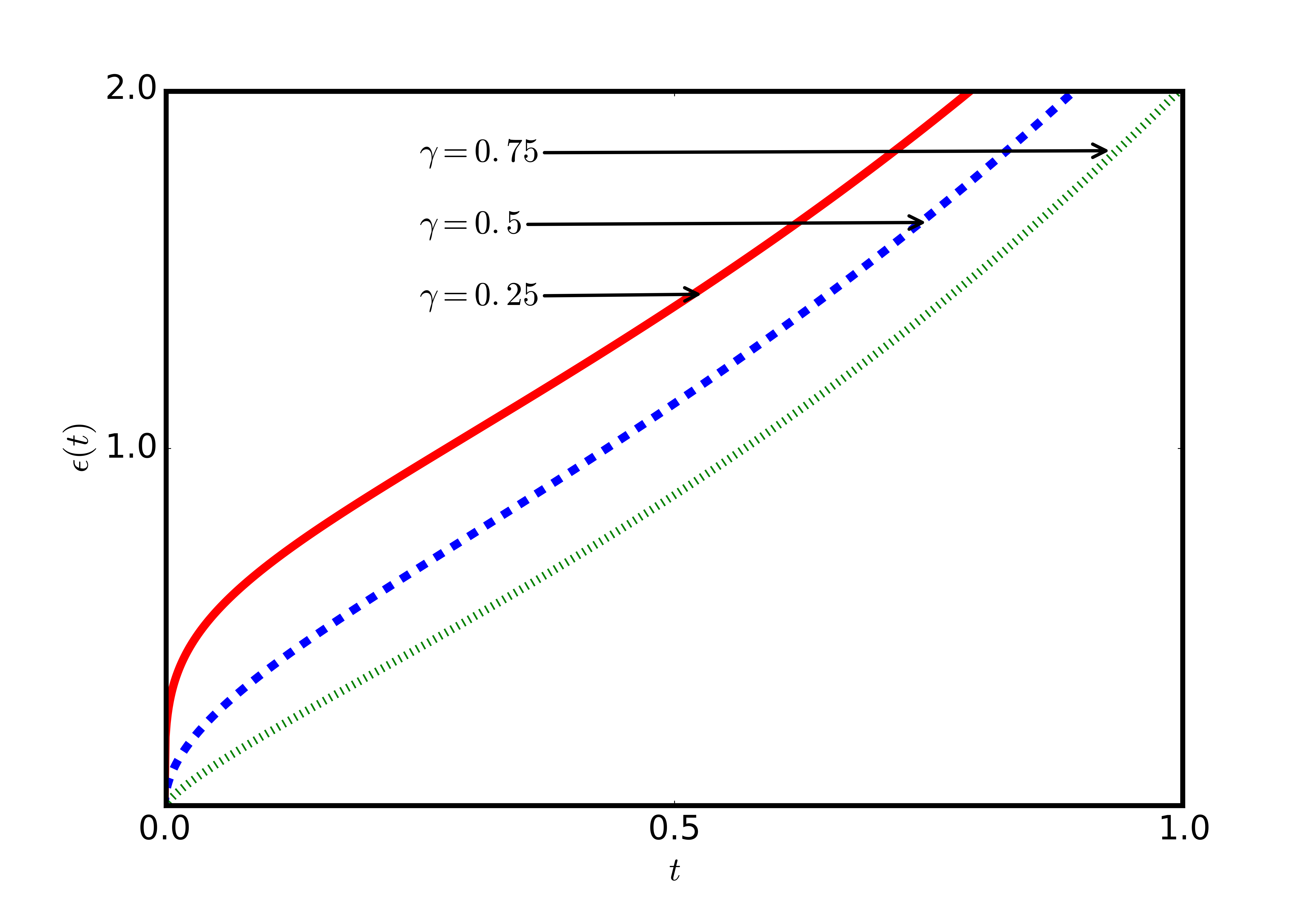
Figure 1. Plot of the strain response to the creep experiment in (3.3), setting $\sigma_{0}$, $\tau$, $\eta_{0}$ and $\alpha$ to one.

We recall that this classical rheological model interpolates the pure solid behaviour for $\gamma=0$ and the Newtonian fluid for $\gamma=1$.

From an experimental perspective, it is worth noting that this specific implementation of the Scott-Blair model with time-varying viscosity has been used, by the same authors, to characterize the damage growth during creep tests for salt rock samples, see [22].

Now, our proposal is to use a different mathematical approach based on the technique discussed in Section 2. Indeed, let us consider a constitutive equation given by

(3.4) $$\sigma(t)=\eta_{0}\,\tau^{\gamma-1}\,\mathcal{D}^{\gamma}\epsilon(t)\,,\quad\mathcal{D}^{\gamma}\equiv{}^{C}\left(\frac{1}{f^{\prime}(t)}\frac{d}{dt}\right)^{\gamma}\,,$$

with $\gamma\in[0,1]$ and for some $f(t)\in C^{1}(\mathbb{R}^{+})$ strictly increasing function for all $t>0$, i.e. $\mathcal{D}^{\gamma}$ is defined according to (2.2) with $a=0$ and $b=+\infty$.

Thus, here the idea is to include the effect of the time dependence of the viscosity coefficient in the definition of the fractional operator.

Now, using the results of Section 2, one can infer the general solution of the creep experiment for a material described by the constitutive equation (3.4). Indeed, once set $\sigma(t)=\sigma_{0}$, the general solution of (3.4) reads

(3.5) $$\epsilon(t)=\frac{1}{\Gamma(\gamma+1)}\frac{\sigma_{0}}{\eta_{0}\,\tau^{\gamma-1}}[f(t)-f(0+)]^{\gamma+1}\,.$$

Indeed, considering the equation

$$\sigma_{0}=\eta_{0}\,\tau^{\gamma-1}\,\mathcal{D}^{\gamma}\epsilon(t)\,,$$

with the ansatz $\epsilon(t)=\mathcal{N}\,\big{[}f(t)-f(0+)\big{]}^{\beta-1}$, with $\mathcal{N}$ being a normalization constant, using (2.3) one finds

$$\sigma_{0}=\eta_{0}\,\tau^{\gamma-1}\,\frac{\Gamma(\beta)}{\Gamma(\beta-\gamma)}[f(t)-f(0+)]^{\beta-\gamma-1}\,.$$

Since the left-hand side of the latter is time independent, we are forced to set $\beta=\gamma+1$. Thus, solving for $\mathcal{N}$ in the remaining equation one finds $\mathcal{N}=\sigma_{0}/\eta_{0}\,\tau^{\gamma-1}\,\Gamma(\gamma+1)$, that confirms the result in (3.5).

Example 1 (Exponential function).

Let us consider the case with $f^{\prime}(t)=e^{\alpha\,t}$. Then, (3.4) reads

(3.6) $$\sigma(t)=\eta_{0}\,\tau^{\gamma-1}\,\left(e^{-\alpha\,t}\,\frac{d}{dt}\right)^{\gamma}\epsilon(t)\,,$$

where we omitted the ^C for the sake of clarity.

Then, it is easy to see that $f(t)=e^{\alpha\,t}/\alpha+C$ with $C$ being an integration constant. Now, from (3.5) one immediately infers that the general solution for the latter equation is given by (see Figure 2)

(3.7) $$\epsilon(t)=\frac{1}{\Gamma(\gamma+1)}\frac{\sigma_{0}}{\eta_{0}\tau^{\gamma-1}}\left(\frac{e^{\alpha t}-1}{\alpha}\right)^{\gamma+1}.$$

It is worth noting that, again, for $\gamma=1$ we recover the classical solution related to a Newtonian fluid with time-dependent viscosity and for $\gamma=0$ the solid behaviour $\epsilon\sim\sigma_{0}/\eta_{0}$.

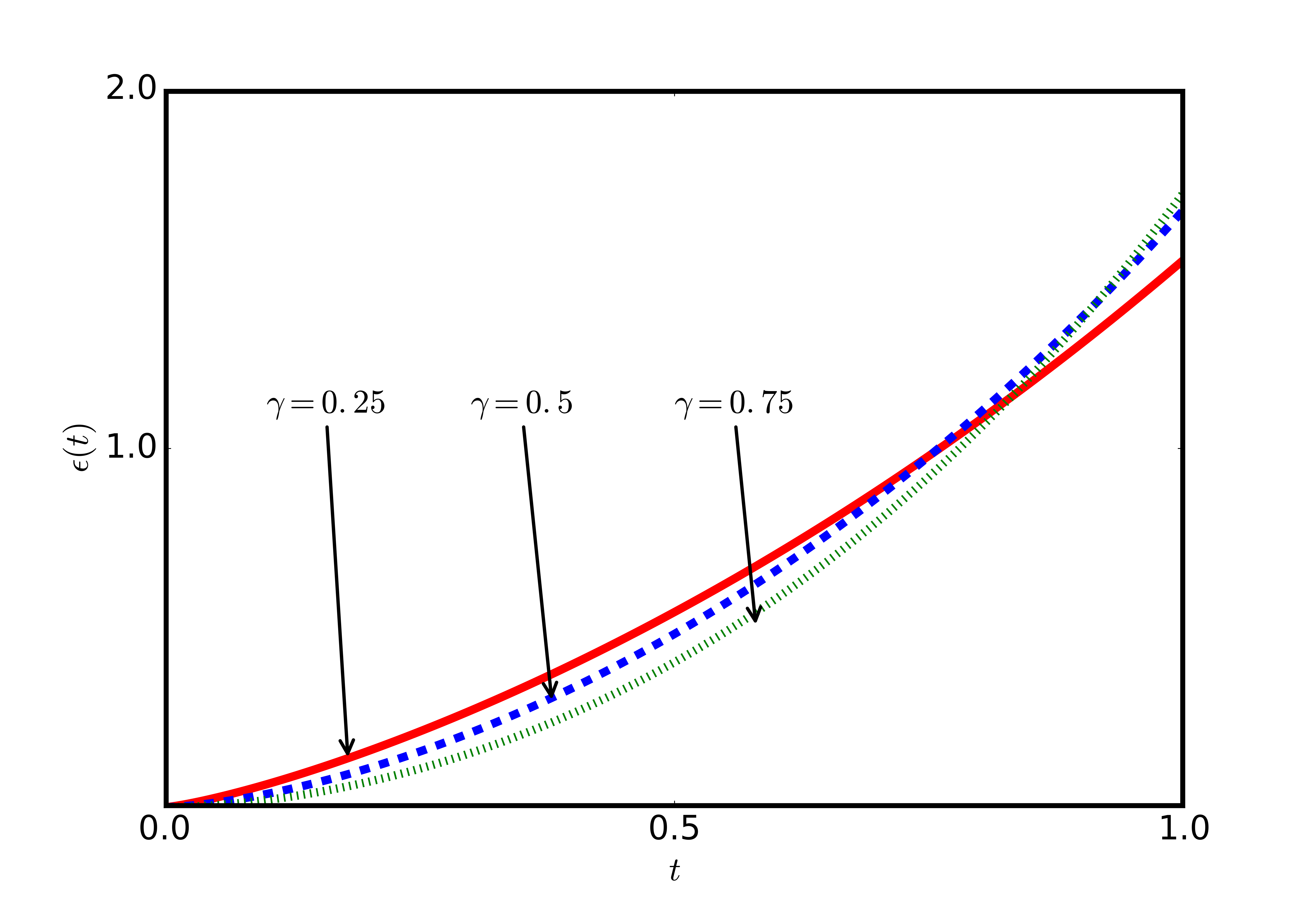
Figure 2. Plot of the strain response to the creep experiment in (3.7), setting $\sigma_{0}$, $\tau$, $\eta_{0}$ and $\alpha$ to one.

Example 2 (Mittag-Leffler function).

Let us now consider the case where

(3.8) $$f(t)=\frac{1}{\alpha}\,E_{\nu}(\alpha\,t):=\frac{1}{\alpha}\,\sum_{k=0}^{\infty}\frac{(\alpha\,t)^{k}}{\Gamma(\nu\,k+1)}\,,\quad\nu\in(0,1]\,,$$

where $\alpha>0$ is a constant such that $[\alpha]=\mbox{time}^{-1}$.

Clearly, the series representation of the Mittag-Leffler function appearing in (3.8) is uniformly convergent for $t>0$ and $\nu\in(0,1]$. Besides, if one preforms the derivative term by term of $f(t)$ it is also easy to see that the resulting series is still uniformly convergent for $t>0$ and $\nu\in(0,1]$, thus one can conclude that

(3.9) $$f^{\prime}(t)=\frac{1}{\alpha}\,\frac{d}{dt}E_{\nu}(\alpha\,t)=\sum_{k=0}^{\infty}\frac{(k+1)(\alpha\,t)^{k}}{\Gamma(\nu\,k+\nu+1)}\,,\quad\nu\in(0,1]\,.$$

The latter, being a series with positive terms, implies $f^{\prime}(t)>0$ for all $t>0$. Besides, it is also easy to see that $f^{\prime}(0+)=1/\Gamma(\nu+1)$.

Then, using the result in (3.5) one finds (see Figure 3)

(3.10) $$\epsilon(t)=\frac{1}{\Gamma(\gamma+1)}\frac{\sigma_{0}}{\eta_{0}\,\tau^{\gamma-1}}\,\left[\frac{E_{\nu}(\alpha\,t)-1}{\alpha}\right]^{\gamma+1}\,,$$

with $\nu\in(0,1]$, $\alpha>0$ and $t>0$.

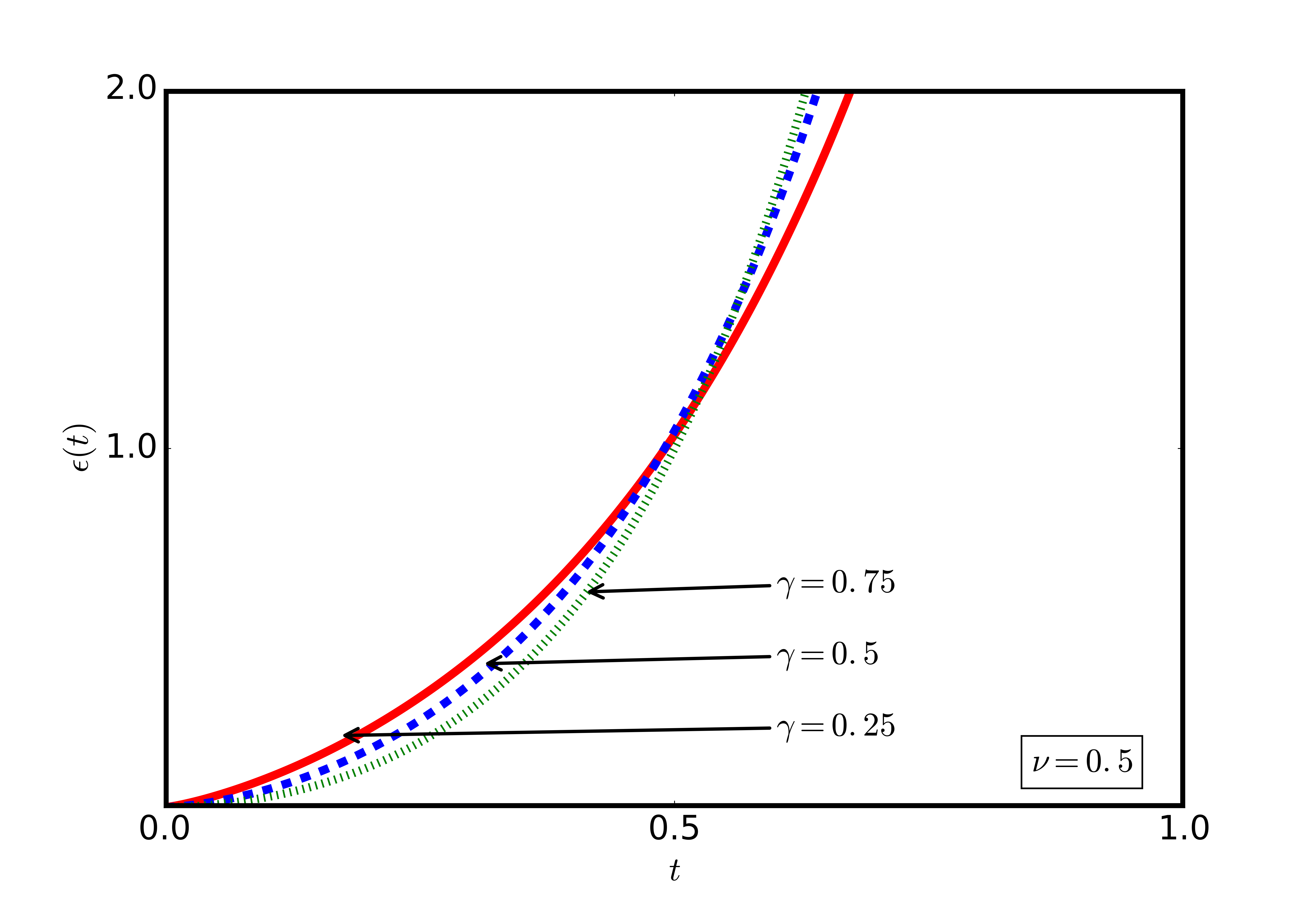
Figure 3. Plot of the strain response to the creep experiment in (3.10), setting $\sigma_{0}$, $\tau$, $\eta_{0}$ and $\alpha$ to one.

Remark.

The plots in Figure 1 and 3 have been obtained by means of a simplified numerical algorithm based on [23, 24].

4. Conclusions

Nowadays, fluids with time-dependent viscosity play a central role in modern material science and engineering. Indeed, this class of shear-thickening non-Newtonian fluids keep being subjected to a shear stress throughout their whole stress history.

In this paper we have suggested an interesting framework whose aim is to provide a simple mathematical scheme to physically model the emergent global structure of these kind of peculiar material.

In particular, after reviewing the general feature of the fractional derivative of a function with respect to another function, we have provided three different example of constitutive equations with time-dependent viscosity by inducing a minimal modification of the renowned Scott-Blair model of linear viscoelasticity.

Thus considering that both the Newton and the Scott-Blair dashpots represent the fundamental building blocks of any standard model of linear viscoelasticity, we strongly believe that the approach presented here deserves some further studies and experimental investigations, as it might have some relevant consequences for the non-linear theory of viscoelasticity.

References

- [1] S. Rogosin, F. Mainardi, George William Scott Blair - the pioneer of fractional calculus in rheology, Communications in Applied and Industrial Mathematics 6 No 1 (2014), e-481, 20 pages.
- [2] M. Stiassnie, On the application of fractional calculus on the formulation of viscoelastic models, Appl. Math. Modelling, 3 (1979), 300–302.
- [3] M. Caputo, F. Mainardi, Linear models of dissipation in anelastic solids, Rivista del Nuovo Cimento (Ser.II) 1 (1971), 161–198.
- [4] F. Mainardi, M. Tomirotti, Seismic pulse propagation with constant and stable probability distributions, Annali di Geofisica 40 (1997), 1311–1328.
- [5] F. Mainardi, Fractional Calculus and Waves in Linear Viscoelasticity, Imperial College Press, London (2010), pp. 340.
- [6] F. Mainardi, G. Spada, Creep, relaxation and viscosity properties for basic fractional models in rheology, The European Physical Journal, Special Topics 193 (2011), 133–160.
- [7] A. Giusti, A comment on some new definitions of fractional derivative, Nonlinear Dynamics, (2018), 7 pages; DOI:10.1007/s11071-018-4289-8
- [8] E. Orsingher, C. Ricciuti, B. Toaldo, Time-inhomogeneous jump processes and variable order operators, Potential Analysis 45 No 3 (2016), 435–461.
- [9] R. Garrappa, Grünwald-Letnikov operators for fractional relaxation in Havriliak-Negami models, Commun Nonlinear Sci Numer Simul 38 (2016), 178–191.
- [10] Sandev T. Generalized Langevin equation and the Prabhakar derivative, Mathematics 5 No 4 (2017), 66.
- [11] A. Giusti, Dispersion relations for the time-fractional Cattaneo-Maxwell heat equation, J Math Phys 59 (2018), 013506.
- [12] H. W. Zhou, et al, Deformation analysis of polymers composites: rheological model involving time-based fractional derivative, Mechanics of Time-Dependent Materials, 21 No 2 (2017), 151-161.
- [13] V. Pandey, S. Holm, Linking the fractional derivative and the Lomnitz creep law to non-Newtonian time-varying viscosity, Phys. Rev E 94 (2016), 032606.
- [14] R. Garra, A. Giusti, F. Mainardi, The fractional Dodson diffusion equation: a new approach, Ricerche di Matematiche, (2018), 11 pages; DOI:10.1007/s11587-018-0354-3
- [15] R. Almeida, A Caputo fractional derivative of a function with respect to another function, Commun. Nonlinear Sci. Numer. Simulat. 44 (2017), 460–481.
- [16] R. Almeida, What is the best fractional derivative to fit data?, Applicable Analysis and Discrete Mathematics 11 No 2 (2017), 358–368.
- [17] R. Almeida, A. B. Malinowska, M. T. Monteiro, Fractional differential equations with a Caputo derivative with respect to a kernel function and their applications, Math. Meth. Appl. Sci. 41 (2018), 336–352.
- [18] M.Jleli, D. O’Regan, B. Samet, Some fractional integral inequalities involving -convex functions, Aequat. Math. 91 (2017), 479–490/
- [19] A. A. Kilbas, H. M. Srivastava, J. J. Trujillo, Theory and Applications of Fractional Differential Equations, Elsevier, Boston (2006).
- [20] G. Pagnini, Erdélyi-Kober fractional diffusion, Fractional Calculus and Applied Analysis 15 No 1 (2012), 117–127.
- [21] R. Garra, A. Giusti, F. Mainardi, G. Pagnini, Fractional relaxation with time-varying coefficient, Fractional Calculus and Applied Analysis 17 No 2 (2014), 424–439.
- [22] H. W. Zhou, et al, A fractional derivative approach to full creep regions in salt rock Mechanics of Time-Dependent Materials 17 No 3 (2013), 413–425.
- [23] R. Garrappa, M. Popolizio, Evaluation of generalized Mittag-Leffler functions on the real line, Advances in Computational Mathematics 39 No 1 (2013), 205–225.
- [24] R. Garrappa, Numerical Evaluation of two and three parameter Mittag-Leffler functions, SIAM Journal of Numerical Analysis 53 No 3 (2015), 1350–1369.