Understanding Flash Crash Contagion and Systemic Risk:
A Micro-Macro Agent-Based Approach

Abstract

The purpose of this paper is to advance the understanding of the conditions that give rise to flash crash contagion, particularly with respect to overlapping asset portfolio crowding. To this end, we designed, implemented, and assessed a hybrid micro-macro agent-based model, where price impact arises endogenously through the limit order placement activity of algorithmic traders. Our novel hybrid microscopic and macroscopic model allows us to quantify systemic risk not just in terms of system stability, but also in terms of the speed of financial distress propagation over intraday timescales. We find that systemic risk is strongly dependent on the behaviour of algorithmic traders, on leverage management practices, and on network topology. Our results demonstrate that, for high-crowding regimes, contagion speed is a non-monotone function of portfolio diversification. We also find the surprising result that, in certain circumstances, increased portfolio crowding is beneficial to systemic stability. We are not aware of previous studies that have exhibited this phenomenon, and our results establish the importance of considering non-uniform asset allocations in future studies. Finally, we characterise the time window available for regulatory interventions during the propagation of flash crash distress, with results suggesting ex ante precautions may have higher efficacy than ex post reactions.

1 Introduction

During the Flash Crash of 6th May 2010, over a trillion dollars were wiped off the value of US companies in an event that has been largely attributed to the rise of algorithmic trading (Kirilenko et al., 2017). Although the circumstances giving rise to the Flash Crash have been intensely studied since 2010, the role played by algorithmic traders in propagating systemic risk through financial networks remains poorly understood. In the context of networks representing the overlap of asset portfolios held by investment funds (hereafter funds), systemic risk arises as a result of price impact (Brunnermeier and Pedersen, 2009). Despite this, over-simplified systemic risk models typically assume non-crisis linear price impact functions (Benoit et al., 2017). Systemic events such as the Flash Crash of 6th May 2010 demonstrate that during crises (conditions of abnormal perturbation when system dynamics are far from equilibrium), price impact can deviate strongly from linearity (Kirilenko et al., 2017). Analyses of flash crashes have found that the market’s ability to facilitate price discovery is strongly dependent on the micro-level behaviour of market participants, in particular those involved in algorithmic trading (CFTC and SEC, 2010; Menkveld, 2016).

In the present work, we simulate crisis price impact due to algorithmic trading with a limit order book (LOB) agent-based model (ABM), calibrated to exhibit extreme transient price impact phenomena such as flash crashes. The micro-model is derived from Paddrik et al. (2012). We combine this micro-level ABM with a macro-level network model of overlapping leveraged asset portfolios held by funds. Our paper presents a novel synthesis of models from both the microstructure and the macroeconomic literatures. We are aware of few related studies that attempt such a synthesis (Gerig, 2015; Torii et al., 2015). We investigate a key interface between the two classes of model by addressing the over-simplified price impact assumptions typical of macroscopic systemic risk models. In reality, asset prices are formed due to the action of individual traders placing limit orders on stock exchanges, and this is true whether the trader is a global bank seeking to reduce position sizes over several days, or a high-frequency trader (HFT, Menkveld, 2016) targeting fleeting profit opportunities lasting fractions of a second. However, assets do not exist in isolation. Rather, they are held within the portfolios of funds. Funds are thus connected to each other by virtue of the assets they hold in common. Similarly, assets are connected to each other by virtue of being held in the same portfolio at a fund (Allen and Babus, 2008). Following established methodology from the macroscopic systemic risk literature (Huang et al., 2013; Caccioli et al., 2014; Cont and Schaanning, 2017), we represent the fund-asset network as a bipartite graph. We extend previous works by controlling network topology with a preferential attachment method (Barabási and Albert, 1999) which allows us to tune the degree of portfolio overlap and hence the connectivity between funds.

When funds borrow from a bank or brokerage to finance an asset portfolio, they are required to maintain leverage (the ratio of portfolio value to collateral) below a pre-agreed limit as the value of the assets in their portfolio varies (Brunnermeier and Pedersen, 2009). If the portfolio value suffers a loss due to price fluctuation, the fund may be required to either deposit additional capital or rapidly liquidate assets (deleverage) in order to satisfy the leverage constraint. This scenario is known as a margin call and can be enacted by the lending bank on a daily or intraday (during trading hours) basis (Gai et al., 2011; Brunnermeier and Pedersen, 2009). Loss to the lender bank accrues when the liquidation value of a client fund’s portfolio is less than the value of the outstanding loans for which the portfolio acts as collateral. In this circumstance, it is impossible for the fund to repay its debt, and the fund defaults. As Brunnermeier and Pedersen (2009) describe, a problematic amplification mechanism known as a margin spiral can occur if a fund is forced to sell its assets due to losses: the action of selling further depresses prices, increasing losses and requires further rounds of distressed selling. Systemic risk arises when different funds have investments in the same assets. Here, distressed selling by a fund causing prices to fall via price impact will cause losses at all other funds with investments in the distressed assets. These other funds may then be required to reduce the size of their investments in order to manage their leverage and so the distress propagates in what is known as a fire sale (Shleifer and Vishny, 2011).

Our hybrid micro-macro ABM allows us to characterise the effect on systemic risk of leverage management policies and fund-asset network topology. In addition to considering systemic stability (characterised by the default of funds on their margin loans), the use of a limit order book ABM allows us to measure the speed at which financial distress propagates between assets over short intraday timescales characteristic of flash crashes. We investigate systemic risk due to (i) portfolio crowding, which is a measure of the similarity of the asset portfolios held by different funds, and due to (ii) portfolio diversification which relates to the number of assets in which funds invest. We further investigate the effects on systemic risk of the amount of leverage and capital deployed by funds, and of the tolerance with which funds manage their leverage under fluctuating asset price conditions. We show how these parameters control liquidity supply due to distressed selling in the limit order book. We also identify conditions under which leverage management practices constitute a sufficient contagion channel for flash crash propagation and default cascades.

Our results contribute to the growing literature on the use of ABMs to investigate the complex, emergent dynamics of financial systems (LeBaron, 2000; Tesfatsion, 2002; Farmer and Foley, 2009; Haldane and May, 2011; Fagiolo and Roventini, 2017; Haldane and Turrell, 2018). ABMs are able to reproduce empirically observed features (stylised facts, Cont, 2001) of financial systems that cannot easily be captured within mainstream Dynamic Stochastic General Equilibrium (DSGE) approaches (Fagiolo and Roventini, 2017). The complex interactions of heterogeneous, boundedly-rational, autonomous agents give rise to emergent phenomena that cannot be predicted from an understanding of agent behaviour alone. However, this expressiveness comes at a cost. ABMs typically feature a large number of parameters, making model calibration difficult and costly in terms of computational resources. It is, furthermore, necessary to perform repeated stochastic Monte Carlo simulations of ABMs in order to build statistical confidence in observed system dynamics (Franke and Westerhoff, 2012). However, the financial crisis of 2007-2009 demonstrated the inadequacy of mainstream DSGE models in analysing the systemic risk of the banking system (Fagiolo and Roventini, 2017). ABMs offer a compelling alternative, and advances in their methodology and in computer power and data availability will further enhance their effectiveness.

This paper proceeds as follows. Section 2 discusses related studies. Section 3 presents our joint microscopic/macroscopic simulation methodology. Section 4 presents an empirical validation of the model. Section 5 presents results demonstrating the effect of distressed selling on asset prices. Results concerning the impact of leverage, capitalisation and margin tolerance on systemic risk are provided in Section 6. The effect of fund–asset network topology on systemic risk is investigated in Section 7. Section 8 concludes the paper and presents further work directions.

2 Related Work

There has been growing recognition of the importance of considering network effects as contributing factors to systemic risk in the financial industry e.g., Gai and Kapadia (2010); Gai et al. (2011); Haldane and May (2011); Acemoglu et al. (2015); Haldane and Turrell (2018). Within this literature, distressed deleveraging (fire sales, Shleifer and Vishny, 2011; Greenwood et al., 2015), has been established as a major channel for financial distress contagion via shared asset holdings (Arinaminpathy et al., 2012; Caccioli et al., 2014, 2015; Battiston et al., 2016; Capponi and Larsson, 2015; Cont and Schaanning, 2017). When funds hold overlapping portfolios of shared assets this is known as crowding (Menkveld, 2015; Sias et al., 2016). Price impact (Tóth et al., 2011; Zarinelli et al., 2015) is critical to understanding the role of position crowding in fire-sale distress. Price impact under distressed market conditions has been shown to exhibit very different properties to price impact under equilibrium conditions (Cristelli et al., 2010). However, as Table 1 illustrates, this aspect of shared-asset models is often treated in a simplified manner. This point is also raised by Benoit et al. (2017). Table 1 presents a range of studies from the macroscopic systemic risk literature, each of which features overlapping asset portfolios as a contagion channel for financial distress. We present the method of price impact calculation deployed in the papers. Although the table features both linear and exponential forms for price impact, the two forms are closely related. As Caccioli et al. (2014, p.238) states, exponential price impact “corresponds to linear market impact for log-prices”. The papers surveyed contain a mix of single- and multi-asset models. Some of these multi-asset models combine assets into representative clusters which are referred to as asset classes. Models with a single asset are unable to investigate the propagation of distress between assets, such as that encountered during flash crashes. Models that use a representative asset class are unable to simulate the price dynamics of single assets and so the details of liquidity provision are precluded from investigation. Finally, we note in Table 1 that the majority of papers surveyed do not consider short selling (the action of borrowing assets to sell in the hope of repurchasing at a lower future price, equivalent to taking negative positions). Such long-only models are therefore precluded from investigating financial distress amplification mechanisms such as the short squeeze (Dechow et al., 2001).

Paper	Price impact	Securities	Investment
Nier et al. (2007)	exponential†	single	long
Gai and Kapadia (2010)	exponential†	single	long
Arinaminpathy et al. (2012)	exponential†	multiple‡	long
Cont and Wagalath (2013)	linear	multiple	long/short
Huang et al. (2013)	linear	multiple	long
Caccioli et al. (2014)	exponential†	multiple	long
Di Gangi et al. (2018)	linear	multiple‡	long
Greenwood et al. (2015)	linear	multiple	long
Caccioli et al. (2015)	linear	single	long
Battiston et al. (2016)	linear	multiple	long
Serri et al. (2016)	linear	multiple	long
Cont and Schaanning (2017)	linear	multiple	long

Table 1: A survey of price impact functions and portfolio investment constraints utilised in shared-asset models of financial contagion. †corresponds to “linear market impact for log-prices” (Caccioli et al., 2014, p.238). ‡represents the set of equities or bonds (for example) by a single representative asset class. Long and short refer respectively to positively and negatively signed investments.

Linear price impact functions fail to capture the emergent and time-dependent nature of market liquidity (the ability to freely buy and sell assets at current prices), the study of which falls within the market microstructure literature (Gould et al., 2013). Events such as the Flash Crash of 6th May 2010 (Kirilenko et al., 2017) demonstrate that price impact during crisis periods can be extreme. On that occasion, asset prices exhibited unprecedented volatility as the orderly provision of market liquidity broke down. The event was also characterised by the high speed at which prices fell and subsequently returned almost to pre-crash levels. Automated algorithmic trading systems were implicated in all phases of the Flash Crash, including triggering the event, sustaining price falls, and facilitating eventual reversals (CFTC and SEC, 2010).

Two key and related mechanisms mean that crisis price impact is different from equilibrium price impact. Cristelli et al. (2010) and Bookstaber and Paddrik (2015) argue that, during crises, market participants refrain from placing orders. Easley et al. (2012) relate this phenomenon to the inferred presence of toxic order flow, i.e. strongly directional price movements that are outside non-crisis bounds. This removal of liquidity leads to sparsely populated LOBs, and as discussed by Farmer et al. (2004), gaps on the LOB can lead to further large price movements.

Recent research has demonstrated the success of agent-based approaches in investigating intraday market stability, and in particular the role of HFT (Menkveld, 2016) in liquidity provision and flash crashes e.g. Hanson (2011); Johnson et al. (2012); Paddrik et al. (2012); Vuorenmaa and Wang (2014); Budish et al. (2015); Jacob Leal and Napoletano (2017). Although these models are successful at reproducing stylized facts of financial markets including during crises, attempts to extend these models to multi-asset or multi-venue settings have been extremely limited.

Kirilenko et al. (2017) and Golub et al. (2012) take purely empirical approaches to understanding the causes of the Flash Crash of 6th May 2010. Kirilenko et al. (2017) use regression analysis on a unique dataset labelled with the identities of market participants. This analysis demonstrated that HFT activity resulted in a “hot-potato” effect exacerbating price declines. Golub et al. (2012) looks at order placement activity in markets one minute either side of mini-flash crash events (Johnson et al., 2012) finding HFTs withdraw liquidity when it is needed most, at the same time as market makers and other liquidity providers.

Hanson (2011), Paddrik et al. (2012), Vuorenmaa and Wang (2014), and Jacob Leal and Napoletano (2017) use combinations of agents representing low and high frequency market participants and are successful at reproducing the characteristic price fall and recovery observed during flash crashes. Indeed, the price recovery observed during flash crashes is another way in which crisis price impact differs from the linear models used in the fire-sales literature. During the Flash Crash of 6th May 2010, financial distress was observed to spread throughout equity and futures markets, making it a systemic event. However, microstructure models typically consider a single asset in isolation and do not incorporate network effects. This is a significant limitation of current approaches, and further research is necessary if the systemic risk due to flash crashes is to be successfully modelled and analysed Hanson (2011); Paddrik et al. (2012); Vuorenmaa and Wang (2014); Jacob Leal and Napoletano (2017).

Microstructure models featuring multiple assets are rare in the literature. Gerig (2015) takes a model of informed (fundamentalist) and uninformed (zero-intelligence) traders across multiple assets and finds that stocks with higher simulated HFT activity are more highly correlated. The authors also find that close price coupling allows pricing errors to propagate more readily. However, the model does not specifically consider network topology, financial stability, systemic risk, or flash crashes. Torii et al. (2015) consider a three-asset agent-based model of arbitrage where an index future (a financial product constructed to track the combined price movement of a set of underlying assets) is traded simultaneously with the set of underlying assets. Torii et al. (2015) find that price shocks can propagate from asset to asset via movements in the index future. The model does not consider the topology of the asset-index network, or flash crashes. However, this is a notable result given the paucity of microstructure models considering the contagion of financial distress. Cespa and Foucault (2014) consider a two-asset model for distress propagation where an “illiquidity cycle” emerges as traders avoid changing their investments when price volatility leads to uncertainty and a reduced “risk appetite”. As with other closed-form approaches, this model does not feature a realistic model of order placement activity.

The purpose of the present paper is to provide a realistic microstructure model of price impact during crisis periods, embedded within a multiple fund, multiple asset environment characteristic of models from the macroscopic systemic risk literature. The model allows us to explore the propagation of financial distress associated with inherently intraday market phenomena such as flash crashes. Events taking place over timescales measured in minutes, seconds, or shorter are simply ignored in the overwhelming majority of macroscopic financial models. However, the impact of such events can, as illustrated by the 6th May 2010 Flash Crash, be measured in trillions of dollars and serve to undermine the orderly functioning of global financial markets.

3 A Micro-Macro Model

Our model features the novel synthesis of a macroscopic fund-asset network with a microscopic limit order book trading simulation. When funds adjust their asset holdings, they do so by placing limit orders in a realistically calibrated stock market model, where heterogeneous trading agents interact with the fund’s orders. Price impact arises endogenously from our simulation, and resulting asset price movements affect the profits and losses of the funds. In order to represent the composite micro-macro structure it is necessary to introduce a set of heterogeneous interacting entities:

1. Banks: to model the provision of leveraged financing to institutions

2. Funds: to model institutions holding leveraged positions in risky assets

3. Assets: to model liquidity provision via the limit order book

4. Traders: to model realistic asset market activity and response to market distress

A summary of the agents and other entities in the model is presented in Figure 1. Dashed arrows indicate secured margin loans extended by the single bank to the fund agents (for the sake of clarity only a small number of funds and assets are represented). Solid arrows represent fund holdings in assets, and this section of the system is what we refer to throughout this work as the “bipartite fund-asset network”. Finally, dotted arrows indicate the order placement activity of the non-leveraged trader agents described in the previous section.

Figure 1: [1.5 COLUMN] Relationships between entities in the model. Arrows represent balance-sheet relationships. Between banks and funds, these relationships refer to secured margin loans and leverage. Between funds and assets, the relationships refer to asset ownership within fund portfolios. Similarly, between traders and assets the relationship again refers to asset ownership in trader portfolios, though in the present model we assume that traders are non-leveraged and so not subject to margin calls. Note that we do not model banks directly investing in assets.

In the sections that follow we will discuss how we capture these entities in our model, but we first present the key assumptions underpinning the present work.

3.1 Assumptions

Before we describe in detail the components of our model, it is first necessary to establish the terms of what the model does and does not set out to simulate.

3.1.1 Asset-related assumptions

Asset microstructure is represented using limit order books. Transactions occur when orders to buy (sell) match against previously submitted orders to sell (buy) (Gould et al., 2013). Our asset model is supported by the following key assumptions.

We assume:

• a single currency for all financial transactions in the model.

• that trading is costless in the sense that there are no commissions, exchange fees or rebates involved in the model. Such costs are likely to be immaterial in comparison to the extreme price impact encountered during flash crash type phenomena.

• that assets have no corporate actions such as splits or dividends (a minor assumption given the timescale of corporate actions is weeks rather than intraday).

• that assets have the same liquidity and trading characteristics, as well as holding the same start price at the beginning of simulation runs. The liquidity assumption can be compared to restricting our asset universe to members of a major index such as the Eurostoxx 50 or S&P 500.

• that assets are not directly linked via derivative contracts such as options or via direct asset–asset ownership. Such links introduce new potential channels for distress propagation and so our model is conservative in this regard.

• that all trading takes place at a single trading venue. Market participant confusion over conflicting data from alternative trading venues was implicated in the Flash Crash of 6th May 2010, and so again our model represents a conservative configuration (CFTC and SEC, 2010).

3.1.2 Fund-related assumptions

Our research questions relate to how the fund-asset network impacts systemic risk (sections 6 and 7), in the present work we therefore do not concern ourselves with how funds build positions first. We characterise the funds in the model as large institutions that take a long time (many days at least) to accumulate positions, and so over the short intraday timescales we wish to consider, such as the duration of a flash crash (minutes), their pre-crisis behaviour is irrelevant to our research questions. However, if a fund enters distress via the enactment of a margin call, it becomes active and seeks to rapidly reduce leverage.

We assume:

• that funds already hold a set of asset positions before the simulation begins and do not adjust positions unless experiencing financial distress.

• that funds do not invest directly in other funds (so-called fund-of-funds). As with asset-asset direct linkage, our model takes a conservative stance in this regard.

• that funds deploy all of their capital as collateral for leverage loans and so have no cash reserves available in order to satisfy margin calls. This implies that funds must liquidate (reduce in absolute terms) asset positions in order to reduce leverage. Capital injection is equivalent to increased margin tolerance, which we investigate comprehensively in the present paper.

• that funds liquidate aggressively (quickly, by taking liquidity), similarly to the empirical observations by Adrian and Shin (2010) and the model by Greenwood et al. (2015).

• that when funds liquidate, they liquidate uniformly across their assets. This approach follows the methodology established by Caccioli et al. (2014).

• that all funds in the simulation have equal starting capital (also as in Caccioli et al., 2014).

• that, in line with established methodology (see Table 1), asset positions are long-only (positive). This strong assumption means that our present work fits into the fire sales literature (Shleifer and Vishny, 2011; Greenwood et al., 2015) and does not attempt to explain long-short phenomena such as the 2007 “Quant Meltdown” (Khandani and Lo, 2007).

3.1.3 Bank-related assumptions

In our model, financial distress propagates between funds connected via shared asset holdings. It is not, therefore, necessary to consider interbank contagion in order to address our research questions. Neither is it necessary for us to represent banks as directly owning assets; this behaviour is encapsulated entirely within funds and so provides a clear separation of responsibilities without loss of generality. Our model thus incorporates a single bank that provides leverage loans to all funds in the simulation.

We assume:

• that all funds in the simulation are offered equal leverage terms, following established methodology (Caccioli et al., 2014).

• that fund portfolio constitution is ignored when banks set leverage limits. In reality, different assets attract different levels of permissible leverage. Increased portfolio volatility reduces the cap and so represents an additional channel of distress propagation. Our model is conservative with respect to this effect, in line with the implicit methodology of related models.

• that banks monitor fund portfolios on an intraday basis and issue margin calls to funds whose current leverage breaches some threshold. This assumption is realistic (Brunnermeier and Pedersen, 2009; Cont and Schaanning, 2017).

• that if a fund defaults (trading losses exceed capital) the bank will take over and liquidate the fund’s portfolio. Margin terms typically provide for this repossession.

• that there are no other funding costs or interest charged by banks to funds. We justify this on the basis of timescale — such fees are, in reality, accounted on a daily or monthly basis and are not material to the short intraday timescales relevant to our research questions.

3.2 Agent-Based Model

In order to simulate the emergent properties of the interconnected, heterogeneous system of banks, funds, assets and traders we implement an agent-based model (ABM). The ABM consists of software agents representing banks, funds and traders. The model further incorporates assets and the markets for the trading of those assets but these are not considered agents in their own right. Our notion of which entities in the model constitute agents follows Wooldridge (2001, p.21):

“An agent is a computer system that is situated in some environment, and that is capable of autonomous action in this environment in order to meet its delegated objectives.”

In the sections that follow we describe the behaviour of, and interconnections between, agents in the model.

3.2.1 Banks

As discussed above, we model the activity of a single bank whose primary purpose is to provide leveraged financing to funds. The bank is modelled by considering its balance sheet of assets and liabilities, in line with existing approaches (Gai and Kapadia, 2010). The balance sheet for the bank in our model is presented in Table 2.

Assets	Liabilities
Margin lending	Loss on margin loans
Cash	Equity

Table 2: Bank balance sheet model. Equity is defined as the sum of assets minus the sum of liabilities.

As shown in Table 2 and discussed previously, we do not model interbank lending in the present work. The function of the bank in our model therefore is to issue debt to funds which is secured using the fund’s initial capital $C^{0}\in\mathbb{R}^{+}$ as collateral. Banks offer funds identical initial leverage $\lambda^{0}_{i}=\lambda^{0},\forall i\in\{1,...,n_{f}\}$, $\lambda^{0}\in\mathbb{R}^{+}$. The total value $L_{i}$ of a loan made by the bank to the $i$th fund is therefore given by $L_{i}=C^{0}_{i}\lambda^{0}_{i}$. This expression demonstrates an important convention regarding leverage: the total cash available to funds for the purposes of investment, $V$, is given by $V_{i}=L_{i}+C^{0}_{i}=C^{0}_{i}(\lambda^{0}_{i}+1)$, so leverage of zero ($\lambda^{0}=0$) corresponds to the case where $L_{i}=0$, that is, no cash is loaned.

As explained above, we assume that each of the $n_{f}$ funds utilise all of their available capital for the purposes of funding asset positions. If we represent the investment of fund $i$ in asset $j$ as elements of a matrix $A_{ij}$ then we may write $C^{0}_{i}(\lambda^{0}_{i}+1)=\sum_{j=1}^{n_{a}}A_{ij}$. If we further represent asset positions as the product of asset price at time $t$, $p_{j}^{t}\in\mathbb{R}^{+}$, and position size in shares, $S_{ij}^{t}\in\mathbb{R}$, then for time $t=0$ we can write $C^{0}_{i}(\lambda^{0}_{i}+1)=\sum_{j=1}^{n_{a}}S_{ij}^{0}p_{j}^{0}$, which makes explicit the relationship between leverage, capital, price and fund asset holdings. As prices fluctuate the total fund portfolio value will also of course vary. This price variation will result in mark-to-market profit and loss at various times accruing to the fund. This profit and loss is combined with the fund’s capital yielding an updated capital at time $t$, $C_{i}^{t}$. We can thus derive the leverage for fund $i$ at time $t$, $\lambda^{t}_{i}$, which is given by

$$\lambda^{t}_{i}=\frac{1}{C^{t}_{i}}\sum_{j=1}^{n_{a}}S_{ij}^{t}p_{j}^{t}-1.$$

As in Cont and Schaanning (2017), we assume that banks continuously measure the ratio $\tau=\nicefrac{{\lambda^{t}}}{{\lambda^{0}}}$ for all funds and issue margin calls when this ratio exceeds a critical hysteresis threshold $\tau_{c}\in[1,\infty)$ (where the infinite limit implies banks never issue margin calls, and the lower limit of 1 implies banks issue margin calls for infinitesimally small fund losses). The margin call state remains in force at a fund until either the fund reduces its leverage $\lambda_{i}^{t}$ such that $\lambda_{i}^{t}<\lambda_{i}^{0}$, or the fund defaults (which occurs when $C^{t}_{i}<0$). Note that in our model the effect of a bank issuing a margin call to a fund is exactly equivalent to a fund managing its leverage to a target – a common industry practice (Cont and Schaanning, 2017). If a fund defaults, we invoke the bank’s realistic prerogative to seize its assets and to continue to liquidate the positions.

Banks act autonomously in their decision as to whether and when to issue margin calls. Although we do not explore bank decision-making in the present work, the possibility justifies our consideration of banks as agents proper in the model.

3.2.2 Funds

The primary purpose of funds in the model is to accept leverage loans from banks and to use these loans to finance a portfolio of assets (see Section 3.2.1). The model incorporates many funds, each with its own randomly allocated portfolio (details of the allocation process are provided below). As asset prices vary as a result of the microstructure simulation described in the next section, so the leverage of funds also varies as profit and loss accrues to the fund’s account. If leverage increases beyond a critical threshold (see Section 3.2.1 for the mathematical details) the fund will enter a margin call state and will aggressively liquidate its portfolio (details of the liquidation mechanism and how this relates to the microstructure model are presented in Section 3.2.4 below). Funds can, in principle, decide autonomously which assets they elect to liquidate. Indeed, Capponi and Larsson (2015) find that the strategic selection of asset liquidation behaviour has a large impact on systemic risk in a macroscopic model. We do not consider this strategic behaviour in the present work. Further fund autonomy manifests in the selection of distressed liquidation parameters, and we explore systemic sensitivity to this in Section 5.

Funds are represented by their balance sheet, as shown in Table 3. As described previously, we do not simulate the acquisition of fund asset portfolios, rather we specify portfolios as part of the initial conditions of simulation runs. This approach allows us to explore portfolios with specific characteristics and their effect on systemic risk.

Assets	Liabilities
Capital	Margin loan
Portfolio of assets	Portfolio profit/loss
	Equity

Table 3: Fund balance sheet model

3.2.3 Fund-Asset Bipartite Network

Following the approaches of Caccioli et al. (2014) and Huang et al. (2013) we define the random bipartite graph (Newman, 2003) $\mathcal{G}=(X\cup Y,E)$ in which edges $E$ represent investments made by funds (bottom nodes, $X$) in assets (top nodes, $Y$) such that $|X|=n_{f}$ and $|Y|=n_{a}$. The structure of $\mathcal{G}$ can be represented by the matrix $A\in\mathbb{R}^{n_{f}\times n_{a}}$, defined in Section 3.2.1. A non-zero element $A_{ij}$ correspond to the presence of an edge $E\in\mathcal{G}$ between fund $i$ and asset $j$. $A$ is thus the adjacency matrix representation of $\mathcal{G}$ (Newman, 2003).

We introduce two parameters to control the topology of $\mathcal{G}$. The fraction of assets in which a fund invests (the diversification, or density, Caccioli et al., 2014) is controlled by parameter $\rho\in[0,1],\rho\in\mathbb{R}$. Funds are restricted such that they hold investments in at least one asset, that is, un-weighted fund degree $k_{\mathit{fund}}=\text{max}(\lfloor\rho n_{a}\rfloor,1)$. Since the same value of $\rho$ is used for all funds, as $\rho\to 1$, all funds converge to the same portfolio (such that every fund invests in every asset). Conversely, $\rho\to 0$ means each fund invests in a single asset.

In order to generate networks with a controllable level of overlap, we introduce the notion of preferential attachment (Barabási and Albert, 1999) governed by a parameter $\beta\in\mathbb{R}$ controlling the non-linear strength of preferential attachment (Krapivsky et al., 2000). Starting with the set of assets, network construction proceeds by adding funds sequentially. Each additional fund makes weighted connections to $k_{\mathit{fund}}$ different assets. The probability that the fund connects with a given asset is related to the total already invested in that asset, modulated by crowding parameter $\beta$. $\beta=0$ generates a fully stochastic Erdős-Rényi random graph (Newman, 2003). $\beta=1$ generates the linear Barabási-Albert model, and $\beta>1$ generates a network in which funds have a very high probability of selecting assets that are already held by other funds. This can leave some assets disconnected from the network in our model, and we account for this in the results that follow. Our model also supports $\beta<0$, which generates networks in which funds prefer to invest in assets with the smallest existing investment. We refer to such network configurations as dispersed. Where $n_{f}\leqslant n_{a}$ it is possible for each fund to invest in a different asset producing a maximally disjoint network with no possibility of contagion between assets. Chen et al. (2014) find that such a network is the most stable configuration in high-leverage scenarios and we seek to test this assertion in our micro-macro model.

Unlike Caccioli et al. (2014), we do not assume that funds make equal investments to each asset in their portfolio. Instead, for each fund we sample $k_{\mathit{fund}}$ random variates from a Gaussian distribution $\mathcal{N}(0,1)$, normalising such that the absolute values of the variates sum to unity. Edges are added between the fund and $k_{\mathit{fund}}$ assets with edge weights assigned in decreasing size order from the set of normalised variates. Algorithm 1 in B presents the network construction method detail.

Figure 2 demonstrates the range of topologies that can be created using our bipartite preferential attachment method (for clarity we present small networks in which $n_{f}=n_{a}=4$). Panels on the same row have equal diversification parameter $\rho$, and panels in the same column have equal crowding parameter $\beta$. Figure 2(a) shows a low density, dispersed configuration in which each fund holds a different asset. This network is disconnected, prohibiting default cascades. As crowding parameter $\beta$ increases in Figure 2(b), the network becomes somewhat more connected with two funds sharing a common asset. The effect of preferential attachment becomes apparent in Figure 2(c) where all funds invest in the same single asset, leaving most assets disconnected from the network. Figures 2(d–f) illustrate higher diversification networks with $\rho=0.5$. In each case the network consists of a single connected component (disconnected assets are not considered to be network components as they are effectively irrelevant to our simulation). It is possible in connected networks for distress at any fund to affect (directly, or indirectly) all other funds. Finally, Figures 2(g–i) demonstrate that as $\rho\to 1$ networks become complete (Newman, 2003). For complete networks it may appear that crowding parameter $\beta$ becomes degenerate, however, for weighted networks this is not necessarily the case. Figures 2(h) and 2(i) demonstrate cases where some nodes receive higher investment than others, even though all nodes have the same (unweighted) degree.

$\rho=0$
	(a)		(b)		(c)
$\rho=0.5$
	(d)		(e)		(f)
$\rho=1$
	(g)		(h)		(i)
	$\beta<0$		$\beta=0$		$\beta>0$

Figure 2: [DOUBLE COLUMN] [IN COLOUR] Illustrative examples of the range of bipartite topologies that can be generated with our network construction method. Top nodes (circles) represent assets, bottom nodes (squares) represent funds. An edge between two nodes represents asset ownership by a fund. Panels on the same row have equal diversification parameter $\rho$, and panels in the same column have equal crowding parameter $\beta$. Darker asset node shading indicates a higher proportional amount invested in the asset.

3.2.4 Traders

Trader agents in our model operate in a single market, single asset capacity in line with the large majority of the ABM micromarket literature. That is, a single trader agent is active in a single asset even though it may be controlled by an entity with interests in multiple assets. Such considerations are of peripheral importance in the present model since funds do not take an active trading role. Trader agents, furthermore, are not considered to be leveraged and so will not be subject to margin calls.

Following well-established principles in the agent-based computational finance literature, we minimise behavioural assumptions by endowing trader agents with minimal intelligence. This approach is known as zero-intelligence (ZI), and is characterised by the lack of forecast capability or adaptation in agents (Gode and Sunder, 1993; Farmer et al., 2005). Despite their apparent simplicity, such models are remarkably successful at reproducing stylised facts of financial markets (Fagiolo et al., 2007; Panayi et al., 2012). To be more specific, we reproduce the model presented in Paddrik et al. (2012) which features a heterogeneous set of trader agents, each of which is in turn based upon behavioural observations of real world trading behaviour on the day of the 6th May 2010 Flash Crash presented by Kirilenko et al. (2017).

Other models were also considered as a basis for the microscopic LOB simulation (Vuorenmaa and Wang, 2014; Hanson, 2011; Jacob Leal and Napoletano, 2017). All of these models feature a combination of low and high-frequency trading and so are broadly similar, but the model presented in Paddrik et al. (2012) had the advantage of removing any strategic choice on the part of agents and by doing so remaining closer to the zero-intelligence principle. Paddrik et al. (2012) has the further advantage of featuring a realistic order matching mechanism which is closer to real-world stock exchanges than any of the other models mentioned above.

As in Paddrik et al. (2012), we assume agents arrive at the market according to a Poisson process with a characteristic mean interaction interval specified per agent type (see Table 4). This approach is standard for micromarket models (Farmer et al., 2005).

Type	Timescale	Inventory (shares)	Population	Inputs
Small	7200s	$(-\infty,\infty)$	6500	–
Fundamental B/S	60s	$(-\infty,\infty)$	2500	toxic order flow
Opportunistic	120s	$[-120,120]$	1600	stochastic signal
Market Maker	20s	$[-120,120]$	320	toxic order flow
HFT	0.35s	$[-120,120]$	16	LOB imbalance
Distressed	10s	$(-\infty,\infty)$	$[1,n_{f}]$	market volume

Table 4: Trader agents in our model are based on Paddrik et al. (2012)’s model, which was calibrated to real market data presented by Kirilenko et al. (2017).

We summarise the main features of the trader agents in Table 4. Detailed descriptions of the trader agent types are provided in A and are closely related to the implementations described in (Paddrik et al., 2012). However, the present model enhances the role of distressed selling agents from Paddrik et al. (2012). The connection between the behaviour of the distressed selling agent and the liquidation behaviour of a controlling fund agent is discussed in the next section.

3.2.5 Distressed Sellers

A single aggressive seller executing a large set of trades was identified as a key causative factor in the 6th May 2010 Flash Crash (Kirilenko et al., 2017). Distressed seller agents place market orders (orders with quantity but no price limits) with an order size limited to a fixed percentage of the previous one-minute trading volume. This facilitates a positive feedback loop if the placement of such orders causes market volume to increase, leading to the placement of even larger orders as observed in the 6th May 2010 Flash Crash. The distressed sellers in our model come from two sources:

1. Exogenous distressed sellers, introduced to shock the system, and

2. Distressed sellers implementing the liquidation order placement of distressed funds.

First, as in (Paddrik et al., 2012), we introduce a distressed seller with a given position size at a specific time point in the simulation purely to generate an asset price shock. We allow a period of 20% of the simulation duration to elapse before shocking assets to allow initial transient effects to decay. This distressed seller will continue to attempt to liquidate until it has sold its entire position, after which point it becomes inactive. The second source of distressed sellers in our model are distressed funds. When a fund is in a margin call or default state it is compelled to reduce leverage by liquidating asset positions. We model this by introducing a distressed seller agent to the market for every asset that the fund chooses to liquidate (in the present work, this is all assets held by the fund). The distressed seller attempts to reduce its parent fund’s position in each asset to zero. Critically, however, if fund leverage falls back below the tolerance threshold, liquidation is suspended, and the distressed agents representing the fund are deactivated. It is possible that the fund may re-enter distress later and here the distressed selling agents would reactivate. Our justification for this deleverage mechanism is that margin call terms usually stipulate that leverage must be brought under control within a single trading day, thus necessitating immediate and robust action (Brunnermeier and Pedersen, 2009).

3.2.6 Assets

Assets are not treated as agents in the model. Rather, assets represent the environment in which the other agents are situated (Wooldridge, 2001). Assets can be bought and sold by trader agents utilising market and limit orders via a realistic continuous double auction matching engine. The market clears according to the industry-standard price-time priority (Gould et al., 2013), and agents are able to view the current state of the market as represented by the LOB. Matched orders results in a trade, and the current price of the asset is thus deemed to have been updated. The simulation is enhanced by the realistic inclusion of an opening auction period and intraday volatility auctions. In both of these situations, market clearing is suspended for a period of time to allow liquidity to accumulate on the LOB and hence aid price discovery. We assume an initial one-minute opening auction phase and trigger realistically calibrated five-second volatility auctions when prices fall by 1.3% in a single second, after Paddrik et al. (2012).

3.3 Systemic Risk Metrics

For a comprehensive survey of systemic risk metrics the reader is referred to Bisias et al. (2012) and Acharya et al. (2017). For the present work we adopt two notions of systemic risk. The first is tailored to distress at funds, and the second is tailored to distress in assets.

3.3.1 Financial Contagion

We have available several measures of fund distress: 1) fund profit and loss, 2) funds entering margin call state, and 3) funds defaulting (when losses exceed capital). In the analysis that follows we adopt funds entering default as our fund-level systemic risk metric. The advantage of this metric is that it represents an extreme situation, more-so than merely entering margin call state, and also represents a terminal state of the fund (funds do not participate further in the simulation once they are in default). Using profit and loss would require the specification of the value of loss necessary to describe a fund as distressed. By using the notion of default we automatically calibrate this threshold (the relationship between profit/loss and default is stated in Section 3.2.1).

Following Caccioli et al. (2014) we measure financial contagion by considering the fraction of funds that enter default in each simulation run. If at least $\gamma=5\%$ of funds are in default by the end of the simulation, we join Caccioli et al. (2014) in considering a default cascade to have occurred. We define the probability of contagion as the fraction of Monte-Carlo trials (see Section 3.4) in which a default cascade occurs. Again following Caccioli et al. (2014), we define the extent of contagion as the fraction of funds in default, conditional on a default cascade having occurred. Formally, the probability of contagion is given by

$$P_{\mathit{contagion}}=\frac{1}{M}\sum_{m=1}^{M}\mathbb{I}_{\mathit{cascade}}(m),$$ (1)

where $M$ is the number of Monte-Carlo trials for a single location in the parameter space. $\mathbb{I}_{\mathit{cascade}}(m)$ is an indicator variable representing the occurrence of a default cascade during trial $m\in[1,M]$, and is defined as

$$\mathbb{I}_{\mathit{cascade}}(m)=\begin{dcases}1&\mathrm{if}\enskip f_{\mathit{default}}(m)>\gamma,\\ 0&\mathrm{otherwise},\end{dcases}$$ (2)

where $\gamma$ is a scalar threshold controlling the fraction of funds that must default before we consider a default cascade to have occurred. $f_{\mathit{default}}(m)$, the fraction of funds entering default during Monte Carlo trial $m$, is given by

$$f_{\mathit{default}}(m)=\frac{1}{n_{f}}\sum_{i=1}^{n_{f}}\mathbb{I}_{\mathit{default}}(i,m),$$ (3)

where $\mathbb{I}_{\mathit{default}}(i,m)$ is an indicator variable representing the default of fund $i$ in trial $m$, and is defined as

$$\mathbb{I}_{\mathit{default}}(i,m)=\begin{dcases}1&\text{if fund}\enskip i\enskip\text{defaults in trial}\enskip m,\\ 0&\text{otherwise}.\end{dcases}$$ (4)

The extent of contagion, $\Omega_{\mathit{contagion}}$, is defined by Caccioli et al. (2014) as the expected fraction of funds entering default, given a default cascade occurs. Formally, let us define $\mathcal{D}$, the set of Monte Carlo trials in which a default cascade occurs, such that $\mathcal{D}=\{m\in[1,M]\mathrel{\mathop{\mathchar 58\relax}}\mathbb{I}_{\mathit{cascade}}(m)=1\}$, then we may write

$$\Omega_{\mathit{contagion}}=\frac{1}{|\mathcal{D}|}\sum_{m\in\mathcal{D}}f_{\mathit{default}}(m).$$ (5)

Note that $\Omega_{\mathit{contagion}}$ is undefined if no default cascades occur, i.e. if $\mathbb{I}_{\mathit{cascade}}(m)=0\enskip\forall\enskip m\in[1,M]$, giving $|\mathcal{D}|=0$.

3.3.2 Flash Crash Occurrence

The second systemic risk notion concerns distress at assets, and here again we have a choice of possible metrics. Paddrik et al. (2012) look at the lowest price attained by simulated assets, which has the benefit of simplicity but lacks consideration of the time dimension so characteristic of flash crash phenomena. Although price falls are indeed material to our investigation, our research questions are also concerned with the speed at which distress propagates, and the temporal characteristics of sudden price movements are better-described by metrics that are specifically designed to detect flash crashes. Johnson et al. (2012) consider both price movement magnitude and timescale, but also require an unbroken sequence of trade prices in a given direction (Johnson et al., 2012, p.3):

“For a large price drop to qualify as an extreme event (i.e. black swan crash) the stock price had to tick down at least ten times before ticking up and the price change had to exceed 0.8%. … In order to explore timescales which go beyond typical human reaction times, we focus on black swans with durations less than 1500 milliseconds”

We encountered difficulty calibrating Johnson et al. (2012)’s method. In particular the metric was not found to be robust to simulation scaling (Section 3.4).

Vuorenmaa and Wang (2014) define a flash crash as a price fall of 10% followed by recovery of at least 50% of the size of the fall over an unspecified short timescale. Jacob Leal et al. (2016) use a similar metric based on a price fall of 5% followed by an unspecified degree of reversion within a period of 30 minutes. The dependence on price reversion in each of these metrics was found to be problematic for our model where prices may not revert within the simulated timescale.

We define a flash crash as a price fall of 5% over a rolling 5-minute window. No further constraints are applied. This metric was found to be robust to simulation scale, and to provide a better false positive rate than using the occurrence of volatility auctions (triggered by falls of 1.3% in a single second, see Section 3.2.6). Formally, let us define a variable, $\mathbb{I}_{\mathit{FC}}$, indicating the presence of a flash crash in asset $j\in[1,n_{a}]$ at time $t\in[1,T]$, as

$$\mathbb{I}_{\mathit{FC}}(j,t)=\begin{dcases}1&\frac{(p_{j}^{t}-p_{j}^{t^{\prime}})}{p_{j}^{t^{\prime}}}<-0.05,\\ 0&\text{otherwise},\end{dcases}$$ (6)

where $p_{j}^{t^{\prime}}$ is the price of asset $j$ at $\text{max}(t-5\enskip\text{minutes},0)$.

3.3.3 Flash Crash Propagation Speed

In addition to considering the fraction of assets experiencing flash crashes according to the above definition, we also consider the speed of flash crash propagation through the system. Propagation speed is only well-defined where the number of assets experiencing flash crashes is at least two. We measure the time since the start of the simulation run at which assets experience their first flash crash (individual assets may go on to experience several flash crashes but we do not need to account for this in our propagation speed metric). We then sort these time intervals in ascending order and take the time difference between the first flash crash and the 80th percentile flash crash as a measure of the time taken for flash crash propagation in the system. We scale this time interval inversely according to the number of assets that experience flash crashes, giving a resulting metric with units of flash-crashes per minute.

Let us define the set $\mathcal{F}^{j}$ of flash crashes experienced by asset $j$ such that $\mathcal{F}^{j}=\{t\in[1,T]\enskip\mathrel{\mathop{\mathchar 58\relax}}\enskip\mathbb{I}_{\mathit{FC}}(j,t)=1\}$, where $T$ is the total number of simulated time steps, and $\mathbb{I}_{\mathit{FC}}(j,t)$ is the indicator variable defined above.

Let us further define a total order $\leq_{j}$ over $\mathcal{F}^{j}$, then we may label the elements $t^{j}_{i}\in\mathcal{F}^{j}$ with indices $i\in[1,|\mathcal{F}^{j}|]$ such that $t^{j}_{1}\leq_{j}t^{j}_{2}\leq_{j}...\leq_{j}t^{j}_{i}\leq_{j}...\leq_{j}t^{j}_{|\mathcal{F}^{j}|}$. We define the set $\mathcal{F}$ of first flash crashes experienced by each asset in a single Monte Carlo trial as

$$\mathcal{F}=\bigcup_{j=1}^{n_{a}}\{t^{j}_{1}\}.$$ (7)

We also define a total order $\leq$ over $\mathcal{F}$. We label the elements $t_{i}\in\mathcal{F}$ with indices $i\in[1,|\mathcal{F}|]$ such that $t_{1}\leq t_{2}\leq...\leq t_{i}\leq...\leq t_{p}\leq...\leq t_{|\mathcal{F}|}$, where $p$ is the index of the $\zeta$th fractile of the ordered set, i.e. $p=\lfloor\zeta|\mathcal{F}|\rfloor$. We fix $\zeta=0.8$ in the present work. Finally, we define the speed $s$ of flash crash propagation by

$$s=\frac{c\zeta(|\mathcal{F}|-1)}{(t_{p}-t_{1})},\quad|\mathcal{F}|>1,$$ (8)

where $c$ is a dimensionless constant that allows us to convert from units of $\text{(time steps)}^{-1}$ to $\text{(minutes)}^{-1}$. If $\delta t$ is the duration of one simulated time step in milliseconds, we have $c=60,000\delta t^{-1}$.

An important feature of this metric is that it smooths out propagation speed for a given MC trial. We observed that propagation speed exhibits non-uniform temporal structure including bursts of activity. However, we also observed that the speed results are noisy and depend strongly on network topology (we return to this matter in Section 7). The smoothing implicit in this metric therefore yields a more robust estimate of the propagation speed than naively using the maximum speed attained in a given trial.

3.4 Simulation Protocol Summary

Our simulation proceeds according to the following steps:

1. Setup (meta): Exogenous selection of parameter space region to explore and the number of stochastic Monte-Carlo (MC) trials to perform for each parameter setting. MC instances dispatched to high-performance computing cluster.

2. Setup (per-trial): Construction of agents with stochastic parameters determined via pseudorandom number generation, including fund–asset network construction.

3. Intraday model: Simulate $T=100,000$ periods of market activity, each step lasting $\delta t=50$ milliseconds.

4. Single period: Agents are selected for order placement according to a Poisson process. LOBs are updated in industry standard price-time priority.

5. Shock: After $T^{*}=\lfloor 0.2T\rfloor$ periods to allow for the decay of initial transient effects, a distressed selling agent is introduced for a single asset. Observation of subsequent system dynamics and measurement of systemic risk.

6. Distributional outputs: Repeated stochastic MC trials facilitate the collection of distributional results.

Due to the stochastic, path-dependent nature of the model (a common feature of agent-based models), it is necessary to perform repeated experimental trials in order to build statistical confidence in the observed systemic dynamics (Fagiolo et al., 2017; Franke and Westerhoff, 2012). This approach, widely known as Monte-Carlo (MC) sampling, induces a considerable computational burden. Our simulation protocol accommodates the computational cost in two ways — firstly by making highly-parallel use of a distributed high-performance computation cluster, and secondly by introducing judicious granularity into the agent simulation. Facing similar computational constraints, Paddrik et al. (2012) introduce granularity by scaling the number of trader agents in their simulation. Table 4 gives unscaled agent populations. Following Paddrik et al. (2012) we divide these populations by a factor of 32 (we found our systemic risk metrics were robust to simulation at $\nicefrac{{1}}{{32}}$ or $\nicefrac{{1}}{{4}}$ scale). Since this scaling results in reduced LOB volume, it is also necessary to scale agent inventory limits by the same factor. Agent activity timescales and order placement sizes are not scaled. We adopt the same time granularity used in the flash crash model of Vuorenmaa and Wang (2014) and set $\delta t=50\text{ms}$. It is possible that the Poisson arrival processes governing agent timing result in more than one agent being selected to place orders on a single LOB during a single time period. In such cases, agent activation order is randomised. Since agents are therefore unable to have perfect knowledge of the LOB at the exact time of their order placement, this randomisation places a lower-bound on agent trading latency. The most active agents (HFTs) arrive at the market according to a characteristic timescale of 350ms (see Table 4), about an order of magnitude slower than the minimal order placement latency supported in our simulation.

3.5 Mathematical Notation

Table 5 presents a summary of the parameters used in this paper. The sampled domain for each parameter is discussed at point of parameter usage in the results sections that follow. Table 6 summarises other non-parameter notation.

Symbol	Name	Theoretical Domain	Sampled Domain
$n_{f}$	Number of funds	$\mathbb{N}^{+}$	$[0,195]$
$n_{a}$	Number of assets	$\mathbb{N}^{+}$	$[1,195]$
$A_{ij}$	Asset portfolio values ($n_{f}\times n_{a}$)	$\mathbb{R}$	$[0,\sim\$100mn]$
$S_{ij}$	Asset portfolio positions ($n_{f}\times n_{a}$)	$\mathbb{N}^{+}$	$[0,\sim 100,000]$
$M$	Number of Monte Carlo replicates	$\mathbb{N}^{+}$	$[1,100]$
$T$	Number of simulated time steps	$\mathbb{N}^{+}$	100,000
$\delta t$	Time step duration / milliseconds	$\mathbb{N}^{+}$	50
$\rho$	Erdős-Rényi network density	$[0,1]$	$[0,1]$
$k$	Network degree of fund nodes	$\mathbb{N}$	$[1,195]$
$\sigma$	Standard deviation of Erdős-Rényi degrees	$[0,\infty)$	0.001
$\beta$	Preferential attachment coefficient	$\mathbb{R}$	$[-7.5,7.5]$
$\lambda^{0}$	Initial fund leverage	$\mathbb{R}^{+}$	$[1,20]$
$C^{0}$	Initial fund capital /$millions	$\mathbb{R}^{+}$	$[0.25,5]$
$\tau_{c}$	Margin hysteresis critical value	$[1,\infty)$	$[1.001,1.2]$
$\bm{\theta}$	Parameter triple $(\lambda^{0},\tau_{c},C^{0})$	-	-
$\alpha$	Fund portfolio uniformity coefficient	$[0,1]$	$[0,1]$
$\eta$	Distressed seller volume fraction	$\mathbb{R}^{+}$	$[0.05,0.18]$
$\delta$	Distressed seller timescale / s	$\mathbb{R}^{+}$	$[1,60]$
$\gamma$	Default cascade indicator threshold	$(0,1]$	0.05
$\zeta$	Flash crash speed measurement percentile	$[0,1]$	0.8

Table 5: Parameters in the model. The sampled domain for each parameter is discussed at point of parameter usage in the results sections.

Symbol	Name	Theoretical Range
$V_{i}$	Total investment value for fund $i$	$\mathbb{R}^{+}$
$L_{i}$	Total loan value made to fund $i$	$\mathbb{R}^{+}$
$p_{j}^{t}$	Price of $j$th asset at time $t$	$\mathbb{R}^{+}$
$Q_{j}^{\mathit{bid}}$	Total shares of $j$th asset at best bid price	$\mathbb{N}^{+}$
$Q_{j}^{\mathit{ask}}$	Total shares of $j$th asset at best ask price	$\mathbb{N}^{+}$
$P_{\mathit{contagion}}$	Probability of contagion	$[0,1]$
$\Omega_{\mathit{contagion}}$	Extent of contagion	$[0,1]$

Table 6: Other notation used in this paper.

4 Empirical Validation

Figure 3(a) demonstrates the output from a single evaluation of the ABM in which we simulate a single asset and a single fund. The simulation comprises $T=100,000$ time steps each representing $\delta t=50$ms for a total of approximately 1.5 hours of simulated trading. The simulation was performed at $\nicefrac{{1}}{{4}}$ scale following the method established by Paddrik et al. (2012).

The system is shocked after an initialisation period at $t=20,000$ by forcing the fund to liquidate all of its inventory. The initial asset holdings of the shocked fund and its liquidation behaviour are calibrated to generate equivalent sell order placement activity to that exhibited by the distressed trader in the 6th May 2010 Flash Crash (Kirilenko et al., 2017). Figure 3(a) shows the price evolution of the system (black, left hand axes) and the one-minute binned trade volume (red, right hand axes). We can see the characteristic crash and recovery signature of a flash crash occurring around $t=60,000$. Market volume and market volatility both increase while the distressed selling is taking place and return to pre-crash levels after the distressed selling has concluded. The zero-intelligence nature of the trader agents precludes any temporally-extended response to volatility and so, unlike in the real Flash Crash of 6th May 2010, the model does not capture the extended period of volatility that followed the real crash (Kirilenko et al., 2017).

Figure 3(b) shows the total volume on the LOB during the simulation disaggregated into bid (black) and ask (red) volumes. We can see that the available bid volume collapses following the introduction of the distressed selling agent at $t=20,000$. As discussed in Section 3.2.4, the distressed selling agent places sell market orders which aggressively remove liquidity from the bid side of the LOB. This figure clearly shows the cause of the eventual flash crash — just before $t=60,000$ there is a brief period where buy-side liquidity collapses to almost zero. In such a regime, the orderly provision of liquidity to the market has failed, and stub quotes (orders placed far from prevailing prices that are not intended to transact) may be executed. This is because market orders do not have price limits and so trades can occur at arbitrarily low prices (Cristelli et al., 2010). Once the distressed selling has completed after $t=60,000$, buy side volume returns to pre-distressed levels, and fundamental buyer agents are able to restore the price to pre-crash levels.

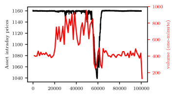
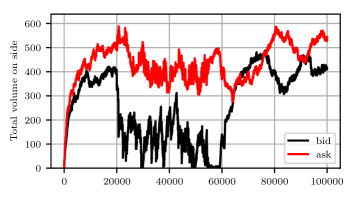
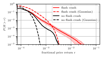
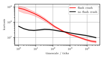
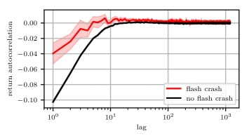
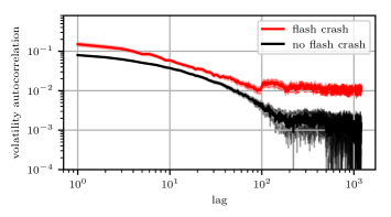
(a) (b) (c) (d) (e) (f)

Figure 3: [DOUBLE COLUMN] [IN COLOUR] Sample model output for a single asset. (a) price and volume series demonstrating the occurrence of a flash crash event. (b) Total volume on bid (black) and ask (red) sides of the LOB demonstrating the collapse of buy-side volume prior to the flash crash. The simulation lasts for $T=100,000$ $\times$ $\delta t=50$ms simulated time steps, therefore represents approximately 1.5 hours of market activity. (c) cumulative distribution function over price returns (log-log scale). (d) return kurtosis measured over increasing time horizons (log-log scale). (e) demonstrating lack of autocorrelation of price returns except at very short horizons (x-axis log scale). (f) demonstrating slowly-decaying autocorrelation of volatility (log-log scale). For panels (c)-(f) we plot the mean across 160 Monte-Carlo trials with 95% confidence interval.

Figures 3(c–f) demonstrate that the model reproduces several important stylised facts of the market (Cont, 2001; Kirman and Teyssiere, 2002; Chen et al., 2012). Figure 3(c) demonstrates that the model produces heavy-tailed returns with a power-law tail. We give the mean cumulative distribution function across 160 Monte-Carlo trials with 95% confidence intervals for trials with (red) and without (black) flash crashes. For comparison, we also show Gaussian return distributions with mean and variance matched to the observed results. Whether a flash crash occurs or not, the returns are heavy tailed. The heavy-tailed nature is much enhanced where flash crashes do indeed occur.

Figure 3(d) demonstrates aggregational Gaussianity (Kirman and Teyssiere, 2002), whereby returns taken over longer time horizons appear more Gaussian and less heavy-tailed. Again, we show 95% confidence intervals around the mean across 160 Monte-Carlo trials disaggregated into trials with and without flash crashes. We plot the kurtosis of the return distribution (a Gaussian distribution has $kurtosis=3$). Both series converge towards the Gaussian kurtosis level as we increase the measurement horizon over 10,000 simulated time-steps, and the decay is significantly more pronounced for trials with a flash crash.

Figure 3(e) demonstrates a lack of autocorrelation of price returns except at very short intraday timescales, and Figure 3(f) demonstrates a long tail in the decay of autocorrelation of volatility (absolute return). Both panels plot mean results across 160 Monte-Carlo trials with 95% confidence intervals. The slow decay of autocorrelation is markedly slower for trials exhibiting flash crash phenomena. These results are consistent with empirically-observed stylised facts (Cont, 2001).

Paddrik et al. (2012)’s model formulation requires all order placement by all agents to be within ten ticks (quantised minimum price increments on the LOB) of the current best price. Their model is therefore precluded from generating the long tailed relative price stylised fact reported by Zovko et al. (2002). A consequence of that modelling decision is that their model does not generate stub quotes. As a result, the Paddrik et al. (2012) flash crash price gradient appears shallow relative to an empirical flash crash or those generated by other models such as Vuorenmaa and Wang (2014). Our model relaxed the ten-tick assumption for the small trader agents only, permitting them to place orders at up to one-thousand ticks away from best. This resulted in an as-expected improvement in the model’s ability to reproduce the relative price stylised fact. Flash crashes generated under this relaxed assumption exhibit a steeper price gradient, in better agreement with empirical data (Figure 3(a)).

For all of these simulations we held-fixed the distressed selling agent properties. Flash crash occurrence is, however, strongly dependent on the price impact of the distressed selling agent’s orders, which we would expect in turn to strongly depend on order size and order placement rate (Paddrik et al., 2012). We explore this matter in the next section.

5 Trading Behaviour and Asset Price Shocks

The distressed selling agent in the Flash Crash of 6th May 2010 reportedly placed market orders sized to not exceed 9% of trailing one-minute market volume (Kirilenko et al., 2017). They furthermore executed a sequence of orders intended to achieve their total desired sell volume over a period of 20 minutes. Although Paddrik et al. (2012) and Paddrik et al. (2015) investigate sensitivity to the volume limit ($\eta$ in our notation), they do not investigate sensitivity to the placement rate ($\delta$ in our notation). We find that flash crash occurrence is critically sensitive to both parameters.

In this experimental scenario we retained the single-fund, single-asset structure adopted in the previous section. The method of shock delivery via the complete liquidation of the fund portfolio is also retained. We performed a combinatorial evaluation over the parameter space $\eta\in[0.005,0.15]$ and $\delta\in[1,60]$ sampling 77 parameter pairs. For each parameter pair we performed 100 Monte-Carlo trials. Each trial was classified according to whether a flash crash was observed in the simulated asset price time-series. We define flash crash occurrence as a price fall exceeding 5% in a period of 5 minutes (see Section 3.3.2 for details regarding this metric).

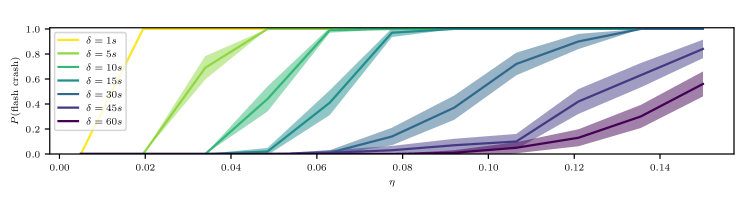
(a) Probability of flash crash occurrence.

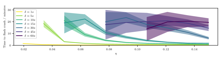
(b) Time interval prior to flash crash occurrence following the onset of distressed selling.

Figure 4: [DOUBLE COLUMN] [IN COLOUR] Single asset flash crash (a) occurrence and (b) time interval prior to occurrence as a function of distressed selling agent properties. $\eta$ refers to the order size limit as a fraction of rolling one-minute market volume. $\delta$ refers to the mean interval between sell order placements in seconds. We show the mean and 95% confidence intervals sampled over 100 Monte Carlo trials.

The mean and 95% confidence intervals for Monte Carlo results are plotted in Figure 4(a). What can be clearly seen in this figure is that flash crashes tend to occur with higher probability as the sizes of orders placed increase, and as the interval between order placements decreases. Both of these findings are consistent with the notion that a flash crash occurs when there is insufficient buy-side liquidity to meet elevated sell-side demand, possibly exacerbated by algorithmic traders withdrawing liquidity from the market. We find that, for any given order size limit in the regime studied, it is possible to reduce the probability of flash crash occurrence by increasing the interval between order placements. Figure 4(a) also demonstrates that for a given order placement interval, $\delta$, there exists a critical value of the order size limit, $\eta$, below which flash crashes occur with negligible probability. Two traders placing equally-sized orders at equal timescales $\delta$ is exactly equivalent to a single trader placing orders with a timescale $\delta^{\prime}=\nicefrac{{\delta}}{{2}}$.

The distressed seller implicated in the Flash Crash of 6th May 2010 reportedly used a value of $\eta=0.09$ (Kirilenko et al., 2017). We calibrate this parameter setting in our model using this reported value, and retain this setting for the remainder of this paper. Although we are not able to calibrate the order placement rate in a similar manner, we select $\delta=10$s as a reasonable setting based on the results in Figure 4(a). Figure 4(b) implies that this choice of $\eta$ and $\delta$ is sufficient to induce a flash crash within approximately two minutes of the onset of distressed selling.

6 Leverage, Capital, and Margin Tolerance

Previous sections have established the effectiveness of the model at reproducing stylised facts of real financial markets, as well as its ability to exhibit flash crashes. We now proceed to consider a full simulation of multiple connected funds and assets, as opposed to the single-fund single-asset simulations studied in previous sections.

In this section, we consider the response of the system to changes in fundamental parameters related to margin tolerance $(\tau_{c})$, leverage $(\lambda^{0})$ and fund capital $(C^{0})$. We find that the multi-asset system exhibits phase changes for critical values of each of these parameters, moving from a stable phase where it is unlikely for fund defaults and flash crashes to occur, to an unstable phase where catastrophic collapse becomes highly likely.

Formal definitions of our systemic risk metrics for fund default cascades and asset flash crash occurrence are given in Section 3.3. In brief, we consider a default cascade to have occurred if more than $\gamma=5\%$ of funds end the simulation in default. We further define the extent of a default cascade to be the fraction of funds in default, conditional on a default cascade having occurred. Both of these metrics follow the methodology of Caccioli et al. (2014). We also introduce our own metric for flash crash occurrence, which we define as an asset price fall of 5% within a rolling five minute window.

6.1 Experiment Parameters

For this experimental scenario we perform a combinatorial exploration over parameter triples $\bm{\theta}(\lambda^{0},\tau_{c},C^{0})$ for $\lambda^{0}\in[1,20]$, $\tau_{c}\in[1.002,1.1]$ and $C^{0}\in[0.1,5.0]$ $millions (210 total combinations). The analysis performed by Ang et al. (2011) suggested that real-world $\lambda^{0}$ typically lies within $[1,20]$ for hedge funds trading equities. Since we do not have access to an independent data source for our calibration, we adopt Ang et al. (2011)’s suggested domain. Analysis of the 6th May 2010 Flash Crash implied the size of sell orders sent by the distressed trader totalled 75,000 (Kirilenko et al., 2017). We sample $C^{0}\in[0.1,5.0]$ such that in combination with $\lambda^{0}$ (see Section 3.2.1 for details), the positions held by funds extend from the region whereby full liquidation of a single fund could not induce a flash crash even if all of its holdings were allocated to a single asset, to the region whereby liquidation of a single fund could indeed induce a flash crash. We do not have access to empirical data on margin hysteresis $\tau_{c}$ and so here we perform a logarithmic sampling across three orders of magnitude in order to determine sensitivity to this parameter. In combination, these parameter domains are sufficient to determine the boundary in $(\lambda^{0},\tau_{c},C^{0})$ space separating stable from unstable behaviour. Each parameter triple, $\bm{\theta}$, is evaluated over five Monte-Carlo trials resulting in a total of 1050 ABM evaluations. Only the pseudorandom number seed is varied between Monte-Carlo trials.

For each evaluation we generate a new set of fund-asset allocations according to the algorithm presented in 3.2.3. Allocations are stochastic with a fixed diversification coefficient $\rho=0.5$ and no preferential attachment ($\beta=0$). The topology may therefore be represented as an Erdős-Rényi random graph (Newman, 2003) in which, on average, edges exist between each fund node and 50% of the available asset nodes. We consider the effect of topology in the next section. Finally, we fix the number of assets and funds at $n_{a}=n_{f}=50$. These selections strike a balance between computational tractability and providing fine enough grained distinction for metrics such as flash crash propagation speed and extent. For the present study, all funds have the same level of capital $C^{0}$ and initial leverage $\lambda^{0}$.

The system is perturbed with an exogenous shock according to the same protocol as that presented in previous sections. We introduce a distressed seller to a single asset (selected from a uniform distribution across all assets that are held by at least one fund). The distressed agent places a sequence of sell orders with a total quantity of shares that is calibrated to trigger a flash crash in the shocked asset. No further exogenous interventions are performed, and further episodes of distressed selling by funds and asset flash crashes arise endogenously.

6.2 Parameter Space Exploration

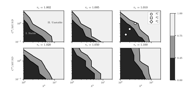
Figure 5: [DOUBLE COLUMN] [IN COLOUR] Probability of contagion as a function of leverage $(\lambda^{0})$, margin hysteresis $(\tau_{c})$ and fund capital $(C^{0})$. Plotted values are the mean across Monte-Carlo trials as a function of $\lambda^{0}$ and $C^{0}$. $\tau_{c}$ increases from panel to panel thus we present slices of the full three-dimensional parameter space at fixed values of $\tau_{c}$. Contour lines are drawn to denote fractional default at the 25% and 75% levels. In region I most funds avoid default, but in region II it is likely that all funds end up in default. In the upper-right panel we label three points in $(\lambda^{0},\tau_{c},C^{0})$ parameter space $\bm{\theta^{\star}_{1}},\bm{\theta^{\star}_{3}},\text{and}\bm{\theta^{\star}_{3}}$. We refer to these in detail in Section 7.

Figure 5 shows the fraction of funds entering default (mean across Monte-Carlo trials) as we perform the combinatorial search. $\tau_{c}$ is increased from panel to panel thus we present slices of the full three-dimensional parameter space at fixed values of $\tau_{c}$. It is clearly seen from this figure that a phase-change exists in leverage-capital space, whereby the likelihood of funds entering default increases from approximately zero (region I) to approximately 100% (region II). This result is consistent with expectations because a larger value of leverage $\lambda^{0}$ magnifies fund losses in response to a given asset price move, making margin calls more likely. This effect is directly mitigated by increasing margin tolerance $\tau_{c}$. Conditional on a margin call being in force, larger fund capital $C^{0}$ means that a greater quantity of shares will need to be sold by the fund, which therefore implies a greater price impact when that fund elects to sell, propagating greater losses to other funds that hold positions in the same assets. Systemic sensitivity to the topological properties of overlapping (crowded) asset portfolios are explored in detail in Section 7.

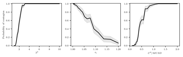
(a) Probability of contagion as we systematically adjust one variable, holding the other two fixed.

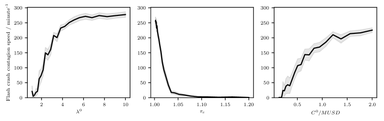
(b) Flash crash propagation speed as we systematically adjust one variable, holding the other two fixed.

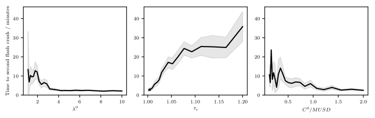
(c) Time taken for the second flash crash to occur following the introduction of the distressed selling agent, as we systematically adjust one variable, holding the other two fixed.

Figure 6: [DOUBLE COLUMN] [IN COLOUR] Exploring financial stability as we systematically adjust one agent parameter, holding the other two fixed. The exogenous variables are Left panels: leverage $\lambda^{0}$, Middle panels: margin hysteresis $\tau_{c}$, Right panels: capital $C^{0}$ (units millions of US dollars, MUSD). We plot the mean across 100 Monte-Carlo trials, along with 95% confidence intervals. The intersection in parameter space is at $\bm{\theta^{\star}_{1}}(\lambda^{0}=3,\tau_{c}=1.01,C^{0}=1)$. The results demonstrate phase changes for each of the three parameters from stable to unstable behaviour.

Although it is not easy to see in Figure 5, a phase change also occurs over the domain of $\tau_{c}$. In order to make this more apparent, we performed linear sensitivity analyses of the three variables in isolation, holding the other two variables fixed. The three sampled lines intersect at $\bm{\theta^{\star}_{1}}=\bm{\theta}(\lambda^{0}=3,\tau_{c}=1.01,C^{0}=1)$. Figure 6(a) plots the probability of contagion for these linear explorations, showing 95% confidence intervals around the mean. This figure clearly demonstrates the phase changes in all three variables under consideration. The change from stability to instability occurs as leverage and capital increase and as margin tolerance decreases. We further observed that the extent of contagion was always 100%, conditional on the occurrence of a default cascade. This result adds evidence in support of existing studies. Similarly to Huang et al. (2013), we find that increasing margin tolerance ($\tau_{c}$) reduces the likelihood of systemic failure, and also that increasing price impact correspondingly increases systemic risk. In our model, price impact is a function of the distressed liquidity entering the market which, by construction, is an increasing function of leverage ($\lambda^{0}$) and capital ($C^{0}$).

Figure 6(b) plots the speed of flash crash propagation for the linear explorations. As discussed in Section 3.3.3, the speed we report here is inversely related to the time taken for 80% of subsequent flash crashes to occur, following the observation of the first flash crash. These results demonstrate that flash crash propagation speed is an increasing concave function of leverage and capital, and a decreasing convex function of margin hysteresis, similarly to the probability of contagion result. Margin hysteresis has a dramatic damping effect on flash crash propagation speed, reducing propagation speeds close to zero for $\tau_{c}>1.03$. These results are straightforward to explain. Increasing leverage makes funds more sensitive to price changes at an asset, making funds more likely to commence distressed selling for a given asset price move, and hence more readily propagating price impact between assets. Increased capital means that, conditional on distressed selling taking place, a fund will sell a larger quantity of shares, resulting in steeper price impact in assets that are being sold. This in turn means that the conditions satisfying our flash crash metric (a fall of 5% within a rolling 5 minute window) will be satisfied sooner than under lower capital conditions. The effect of increasing margin hysteresis is predominantly in opposition to the effect of increasing leverage. However, conditional on flash crashes occurring under high margin tolerance, the total quantity of shares to be unwound will be higher than when tolerance is small. This leads to a mixed effect of the margin tolerance parameter.

Finally, Figure 6(c) illustrates the time taken for the second flash crash to occur following the introduction of an exogenous shock to the system. The first flash crash typically occurs in the asset receiving the exogenous shock, so by measuring the time of the second flash crash we probe the systemic nature of flash crash propagation across the fund–asset network. These results are again consistent with expectations and demonstrate that higher values of $\lambda^{0}$ and $C^{0}$ destabilise the system, causing flash crashes to occur more rapidly following commencement of distressed agent selling. Increasing the margin tolerance $\tau_{c}$ stabilises the system, leading to larger intervals between shock delivery and flash crash onset.

Our model continues to support the conclusions of models with a similarly-structured macroscopic network component. Our work goes further by allowing detailed consideration of distress propagation speeds and of the intraday mechanism by which contagion occurs. Price impact in real markets does not occur instantaneously, rather it manifests across longer time periods while trading strategies are in operation. The realistic calibration of the microstructure component of our model allowed us to show that the market quickly reacts to initial distress, leading to contagious spreading of flash crashes across the network in a matter of minutes. This short time interval places an upper bound on the window for the deployment of ex post regulatory interventions. Our results demonstrate that increasing margin tolerance provides the most effective route to increasing the size of the ex post intervention window. However, the short timescale associated with this window across large regions of the parameter space suggests that ex ante precautions may have higher efficacy than ex post alternatives.

7 Bipartite Network Topology

Previous works such as Acemoglu et al. (2015) and Gai and Kapadia (2010) have established the importance of network topology when considering the systemic risk associated with financial distress propagation. Gai and Kapadia (2010) introduce the notion of robust-yet-fragile networks in which higher network connectivity is advantageous for stability in the presence of small shocks as banks are able to share losses and avoid default. On the other hand, high interconnectedness becomes problematic during high shock conditions by providing a large number of channels for distress propagation. Acemoglu et al. (2015) similarly argue that in low-shock regimes, more highly-connected networks are more stable. In this section we explore the extent to which these findings apply to a joint micro-macro model of systemic risk due to overlapping portfolios.

In Section 6 we represented the fund-asset allocation network as an Erdős-Rényi random graph (Newman, 2003). We held fixed both the topology and the graph density which was characterised by the fund’s average asset diversification $\rho=0.5$. We now discuss systemic risk when network density and topology are varied.

7.1 Experiment Parameters

Using the bipartite network generation algorithm, we construct networks in which funds exhibit varying degrees of asset diversification (controlled by parameter $\rho$) and also varying degrees of preferential asset attachment (controlled by parameter $\beta$).

As in Section 6 where we looked at leverage dependence, we continue with a 50-asset, 50-fund model. We perform a combinatorial set of evaluations for $\rho\in[0,1]$ and $\beta\in[-7.5,-2,0,2,7.5]$ yielding a total of 35 parameter pairs. Each pair was evaluated over 100 Monte-Carlo trials in which only the pseudorandom number generator seed varied between simulation instances.

Based on the results from Section 6 we chose three fixed points in $(\lambda^{0},\tau_{c},C^{0})$ space. These locations are depicted in the upper-right panel of Figure 5 and are presented in Table 7. We performed a total of 10,500 ABM evaluations, each consisting of $T=100,000$ time steps, each step with a simulated resolution of $\delta t=50$ms.

As in previous sections, we introduce an exogenous shock to a single asset in the form of a distressed selling agent, calibrated to place a sequence of orders sufficient to trigger a flash crash in the selected asset. We select the asset to shock uniformly from the set of assets that are held by at least one fund. In this way we avoid shocking assets that are disconnected from the network. Formally, let us define the set of connected assets $\mathcal{A}=\{j\enskip\mathrel{\mathop{\mathchar 58\relax}}\enskip\sum_{i=1}^{n_{f}}A_{ij}>0,\enskip j\in[1,n_{a}],j\in\mathbb{N}^{+}\}$, then the probability of selecting an asset $j^{\prime}\in\mathcal{A}$ as the single asset to receive the exogenous shock is equal to $\nicefrac{{1}}{{|\mathcal{A}|}}.$

	$\lambda^{0}$	$\tau_{c}$	$C^{0}$	leverage regime	stability†
$\bm{\theta^{*}_{1}}$	3	1.01	1	high	typically unstable
$\bm{\theta^{*}_{2}}$	2	1.01	0.5	medium	moderately stable
$\bm{\theta^{*}_{3}}$	1.5	1.01	0.25	low	typically stable

Table 7: Locations in $(\lambda^{0},\tau_{c},C^{0})$ space which are fixed during topology experiments. These points are depicted in Figure 5. †We report the stability at $\rho=0.5,\beta=0,n_{f}=n_{a}=50$, which is consistent with parameter selection in Section 6.

7.2 Probability and Extent of Contagion

Figure 7 presents the probability (left column) and extent (right column) of contagion as we vary network diversification ($\rho$) and crowding parameter ($\beta$). We present results for three leverage scenarios: high leverage ($\bm{\theta^{*}_{1}}$, top row), medium leverage ($\bm{\theta^{*}_{2}}$, middle row) and low leverage ($\bm{\theta^{*}_{3}}$, bottom row). We find that systemic risk is strongly dependent on each of these system parameters.

Figure 7(a) shows that default cascades occur with high probability for all but the smallest values of diversification parameter $\rho$. When $\rho$ is less than 3%, funds invest in a single asset. At low diversification, we find that the system is most stable for dispersed configurations ($\beta<0$). This corresponds to topologies in which each fund invests in a different asset, and so distressed selling by one fund cannot affect the portfolios of other funds (see Table 8). Chen et al. (2014) find a similar result for their purely analytic model. When diversification is low, we also observe that crowded systems ($\beta>1$) are the least stable. This corresponds to a topology in which all funds invest in the same single asset. This has two implications — first that a falling price of this asset will simultaneously affect all funds, and second that distressed selling by any fund will necessarily affect the single jointly-held asset. Both factors contribute to increased price impact at the jointly-held asset and hence flash crash propagation in the system. As diversification increases beyond $\rho=0.03$, the system becomes less stable for all crowding regimes. In high leverage scenarios, we therefore find that increasing diversification does not improve systemic stability. Rather, increased diversification allows contagion to spread freely to more of the assets and funds in the network. Acemoglu et al. (2015) find a somewhat analogous effect when comparing the size of shocks delivered to their system. However, a surprising result emerges as crowding ($\beta$) increases. It is not obvious what mechanism acts to increase system stability as a function of higher portfolio overlap for moderate and high levels of diversification in this high leverage regime. This finding is not consistent with existing literature, and we return to consider it in detail in Section 7.4.

Figure 7(c) presents the probability of contagion in a moderate leverage regime. At very low diversification we again observe that the system is most stable for dispersed configurations ($\beta<0$). We may attribute this finding to the network topology which consists of disjoint sub-graphs in which each fund invests in a single asset, and each asset is held by exactly one fund. We find that cascades cannot propagate as the network is too sparsely connected, similar to the findings by Caccioli et al. (2014). As diversification increases to 5–10% we observe a marked reduction in system stability for all crowding regimes. At this level of diversification the network is sufficiently connected for distress to propagate. However, as diversification increases further we find that systemic risk is reduced which is again consistent with Caccioli et al. (2014), who found that increased diversification means that distress at a fund will be spread between a larger number of assets and so have a smaller effect on any one asset. In the moderate leverage regime, we find that distress at a fund is less likely to cause a flash crash at a given asset. This stands in contrast to the high leverage scenario discussed previously where even fully diversified funds can still have sufficient price impact to trigger flash crash cascades. Highly-crowded regimes ($\beta>0$) also benefit from increased diversification, however such regimes are always less stable than non-crowded regimes. This result is to be expected: when portfolios are strongly-overlapping, distress at a single asset is felt by a large fraction of funds. Distress at a single fund is therefore more readily felt by other funds in crowded regimes.

Figure 7(e) presents results when leverage is further decreased. We find that crowded regimes remain the least stable, regardless of the level of portfolio diversification. However, the figure shows that the benefits of portfolio diversification manifest at lower levels of diversification parameter $\rho$. In particular, no default cascades are observed for $\rho\geqslant 0.75$. When funds utilise low leverage, they are relatively insensitive to price movements of the assets in their portfolios and so even modest levels of diversification are sufficient to avoid the need for funds to engage in distressed selling. In the low leverage regime our results are consistent with those of Chen et al. (2014) who find that systemic risk is minimised when all funds hold the “market portfolio”, which in our notation corresponds to maximum diversification ($\rho=1$).

$\beta$	$\langle n_{f}^{C}\rangle$	95% interval
-7.5	1.52	1.42 – 1.62
-2.0	2.56	2.45 – 2.67
0.0	3.80	3.64 – 3.96
2.0	11.2	10.6 – 11.7
7.5	45.9	45.1 – 46.7

Table 8: Presenting the mean and 95% confidence interval of $n_{f}^{C}$, the number of funds in the largest connected component of the $n_{f}=n_{a}=50$ fund–asset network when $\rho\to 0$, i.e. $k_{\mathit{fund}}=1$, for different choices of crowding parameter $\beta$. Statistics are generated from an ensemble of 100 random networks.

Figures 7(b), 7(d) and 7(f) demonstrate that when default cascades are observed, they typically affect the entire network. That is, the extent of contagion is 100% for anything other than very low levels of portfolio diversification. In the moderate and low leverage regimes the system is “robust-yet-fragile” (Gai and Kapadia, 2010) for higher levels of diversification. Although default cascades are unlikely in such regimes, when they do occur the distress propagation is extensive. In each leverage regime, at low diversification the extent of contagion is highest for more highly-crowded systems. This effect is most pronounced in the moderate leverage regime. In the low leverage regime we did not observe cascades for many parameter combinations and so the (conditional) extent of contagion is undefined (this results in partial series, particularly noticeable in figure 7(f)). When diversification is low, dispersed network topologies can become disconnected. Contagion is limited to the connected component (sub-graph) containing the exogenously-shocked asset, resulting in an extent of contagion of less than 100%.

The presence of “robust-yet-fragile” behaviour creates a problem for policy-makers (Gai and Kapadia, 2010). Although systemic failure can be made less likely by encouraging higher portfolio diversification at funds, if a cycle of deleveraging takes hold, enhanced diversification means that financial distress spreads more extensively through the network of funds and assets, resulting in increased financial damage to the fund sector overall. In the next section we consider the dynamic nature of the spread of distress and investigate the speed of flash crash propagation as a function of network topology.

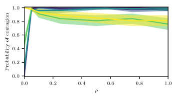
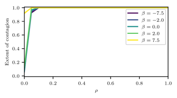
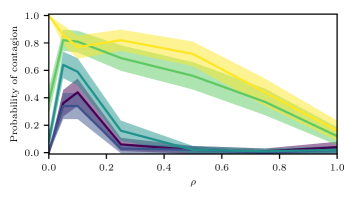
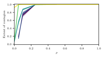
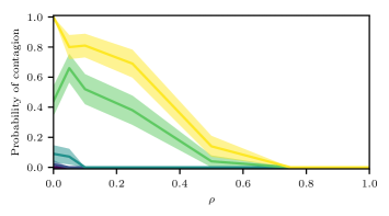
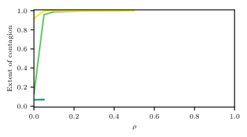
(a) $\bm{\theta^{*}_{1}}$ (high leverage) (b) $\bm{\theta^{*}_{1}}$ (high leverage) (c) $\bm{\theta^{*}_{2}}$ (medium leverage) (d) $\bm{\theta^{*}_{2}}$ (medium leverage) (e) $\bm{\theta^{*}_{3}}$ (low leverage) (f) $\bm{\theta^{*}_{3}}$ (low leverage)

Figure 7: [DOUBLE COLUMN] [IN COLOUR] Probability (a,c,e) and extent (b,d,f) of a default cascade as a function of portfolio diversification ($\rho$) and crowding ($\beta$) parameters. The analysis is repeated for three leverage regimes denoted $\{\bm{\theta^{*}_{1}},\bm{\theta^{*}_{2}}$ and $\bm{\theta^{*}_{3}}\}$ in decreasing order of magnitude.

7.3 Flash Crash Propagation Speed

Figure 8 presents the speed of flash crash propagation as a function of fund and asset diversification in the same three leverage regimes described in the previous section. As mentioned previously, and discussed in detail in Section 3.3.3, the speed we report here is inversely related to the time taken for 80% of subsequent flash crashes to occur, following the observation of the first flash crash.

Figure 8(a) demonstrates that at high leverage, portfolio crowding makes little difference to the speed at which flash crashes propagate between assets. Instead, the speed strongly depends on network diversification ($\beta$, in our notation). The previous section established that under high leverage, enhanced diversification is not beneficial to systemic stability. Figure 8(a) shows that enhanced diversification leads to faster flash crash propagation between assets. The apparent stimulating effect of diversification on propagation speed may indicate that if a set of deleveraging funds wields enough market impact to cause a flash crash in one asset, it likely also wields enough market impact to cause a flash crash in many assets (it is unlikely to have exactly the right level of impact needed to distress one and only one asset) and so enhanced diversification can simply become an enhanced channel for distress propagation. Enhanced diversification also implies that, conditional on entering distress, a fund will send sell orders to a larger fraction of assets in the network. Under high leverage, the resulting price impact causes these assets to undergo flash crashes at similar times during the simulated trading session, resulting in a higher speed measurement. The observed maximum speed of approximately 200 flash crashes per minute corresponds to a time difference of just 5 minutes between the first flash crash and the 80th percentile flash crash. Such a short window places strict constraints on any ex post regulatory interventions, and instead indicates that ex ante measures may be more useful as policy tools.

Figure 8(b) presents flash crash propagation speed results in a moderate leverage regime. Here we find that speed remains low regardless of diversification for non-crowded portfolios. In the previous section we observed that default cascades were unlikely for moderate to high diversification for moderate leverage and low crowding (Figure 7(c)). However, cascades were observed to occur for low diversification in this regime. The low speed at which flash crashes propagate from asset to asset in this case may be due to the fact that the fund-asset network is only sparsely connected, meaning that the effective network diameter (in a graph-theoretic sense) is higher. A higher diameter implies that some assets are more weakly-connected to the network and hence distress takes longer to propagate to such nodes. The results for high-crowding regimes are similar to those for high-crowding regimes at higher leverage, though this observation only holds for low to moderate diversification $\rho$. When $\rho$ increases beyond approximately 50% Figure 8(b) shows that increased diversification reduces flash crash contagion speed. We note that when portfolios are maximally diversified, there can be little difference between crowded and non-crowded configurations (we revisit this notion in the next section), and so it is not surprising that the flash crash propagation speed is similar for crowded and non-crowded topologies when $\rho\to 1.0$. However, it is not obvious why speed should peak near $\rho=0.5$. As density increases from $\rho=0$ to $\rho=0.5$ in crowded regimes ($\beta>0$), the number of assets that have non-negligible levels of investment increases. Crucially, however, at low density the effect of this increase is detrimental to systemic stability (as we saw in the previous section). It is not until density increases further that diversification acts to stabilise lower-leverage systems. It is interesting that the peak of flash crash contagion speed occurs at a higher value of the diversification, $\rho$, than the peak probability of contagion. This could be due to the conditional nature of the speed measurement. Speed is only defined when more than one asset experiences a flash crash, and this is likely highly correlated with cases where default cascades occur. If we only consider cases where default cascades occur, it does not necessarily follow that the speed, under this condition, will be maximised at the same level of diversification as the unconditional systemic stability.

Figure 8(c) presents similar results for a low leverage scenario. Again we see that more crowded systems exhibit higher flash crash propagation speed regardless of portfolio diversification, and that the speed reaches a maximum at an intermediate level of diversification. The figure clearly shows that the maximal propagation speed, for crowded scenarios, occurs at a lower level of diversification coefficient $\rho$ for the low leverage scenario, compared to the moderate leverage scenario. This finding is broadly consistent with Figures 7(c) and 7(e) which find that probability of contagion reaches a maximum for lower values of $\rho$ for low leverage scenarios compared to moderate leverage scenarios. Since flash crash contagion speed is only defined for Monte Carlo trials where at least two assets experience flash crashes, Figure 8(c) features incomplete series.

Taken together, Figures 8(a)-(c) demonstrate that flash crash propagation speed increases as leverage increases. The results also demonstrate that for high-crowding regimes, speed is a non-monotone function of portfolio diversification. The non-monotonicity is related to similar non-monotonicity observed for the probability of contagion in Section 7.2, though the maxima occur at different levels of diversification when considering speed as opposed to stability. We have also found that, similar to the systemic stability results, dispersed configurations and configurations with no crowding have the lowest flash crash propagation speed. This means that they are not only more robust to default cascades, but also that in such scenarios regulators have a larger time window in which to deploy ex post interventions should a deleveraging event occur.

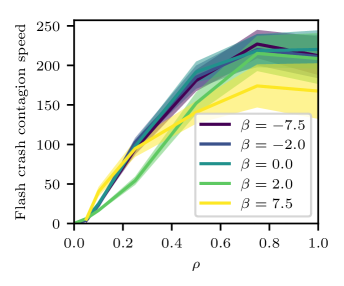
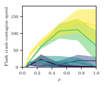
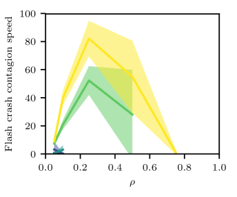
(a) $\bm{\theta^{*}_{1}}$ (high leverage) (b) $\bm{\theta^{*}_{2}}$ (medium leverage) (c) $\bm{\theta^{*}_{3}}$ (low leverage)

Figure 8: [DOUBLE COLUMN] [IN COLOUR] Flash crash propagation speed (minutes^-1)through the fund–asset network as a function of portfolio diversification ($\rho$) and crowding ($\beta$) parameters. The analysis is repeated for three leverage regimes denoted $\{\bm{\theta^{*}_{1}},\bm{\theta^{*}_{2}},\bm{\theta^{*}_{3}}\}$ in decreasing order of magnitude.

7.4 Effect of asset allocation distribution

In Section 7.2 we found the surprising result that in certain circumstances, increased portfolio crowding is beneficial to systemic stability. We are not aware of previous studies that have encountered this phenomenon. It is not apparent in Caccioli et al. (2014) or Chen et al. (2014). In this section we present evidence in support of the hypothesis that the effect is due to the non-uniformity of fund investments between the assets in their portfolio. We thus establish the importance of considering non-uniform asset allocations in future studies.

With reference to Figure 7(a), we consider the probability of contagion in the high leverage scenario $\bm{\theta^{*}_{1}}$. We observe that a higher crowding parameter $\beta$ results in a reduced probability of contagion for most values of portfolio diversification $\rho$, and that this effect becomes more pronounced as $\rho$ increases. This is surprising because $\rho\to 1$ implies that all funds make investments in all assets. The notion of preferentially attaching to a subset of assets therefore has no meaning when funds are simply forced to invest in every asset. This leads us to hypothesise that the non-uniformity of the size of allocations funds make to each asset must have an effect on stability. This would be a potentially important result because a common assumption in the literature is that funds make equal investments in each of the assets in their portfolio, e.g. (Acemoglu et al., 2015; Caccioli et al., 2014).

In order to test this hypothesis, we introduce a parameter $\alpha$ that we use to interpolate between funds holding uniformly-allocated portfolios ($\alpha\to 1$) or Gaussian-allocated portfolios ($\alpha\to 0$). All previous results in the present paper set $\alpha=0$. Figure 9 presents the probability of contagion in the high leverage scenario, at maximum diversification ($\rho=1$ such that all funds invest in all assets), as we vary crowding parameter $\beta\in\{-7.5,0,7.5\}$ and interpolate $\alpha\in\{0,0.25,0.5,0.75,1\}$. For each $(\alpha,\beta)$ parameter pair we performed 100 Monte-Carlo trials, and report the mean and 95% confidence interval from the resulting distribution of default cascade occurrence. As hypothesised, we see that the probability of contagion for different levels of crowding converges as we interpolate from Gaussian to uniform portfolios. This confirms that the surprisingly beneficial impact of increased portfolio crowding in high-leverage scenarios is indeed a result of the non-uniformity of asset allocations in our model.

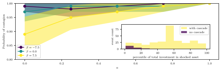
Figure 9: [DOUBLE COLUMN] [IN COLOUR] Probability of contagion with 95% confidence interval as we interpolate between Gaussian-distributed and uniformly-distributed asset allocations for each fund. $\alpha\to 1$ implies funds allocate their capital equally to each asset in which they invest. We fix $\rho=1$ here, such that each fund invests in every asset. This study was carried out in the high-leverage scenario, $\bm{\theta^{*}_{1}}$. Inset: The number of Monte Carlo trials exhibiting a default cascade as a function of the total level of investment in the asset that receives the price shock, for the highly-crowded $\beta=7.5$ case.

Although we have established a connection between portfolio allocation uniformity and systemic risk, we now consider the reason that this connection exists. We hypothesise that the reduced probability of contagion for non-uniform asset allocations in high-crowding compared to low-crowding scenarios is due to the presence of weakly-connected assets in the fund–asset network.

As described in Section 3.2.3, when funds allocate their investments to assets during network construction, they do so in decreasing investment size order. Since the preferential attachment process selects investment targets without replacement, this means that in crowded scenarios ($\beta>0$) funds will tend to allocate their largest investment to the same asset as have other funds. This leads to dispersion in the overall amount invested in each asset. As a consequence, some assets receive significantly higher levels of total investment than others. We might expect that assets with lower levels of total investment are, ceteris paribus, less systemically important than assets with higher levels of investment. This conjecture must hold in the limit $\sum_{j=1}^{n_{f}}A_{ij}\to 0$ for some asset $i\in[1,n_{a}]$ since by definition such an asset is disconnected from the network.

The inset graph of Figure 9 presents the number of Monte Carlo trials exhibiting a default cascade as a function of the total level of investment in the asset that receives the price shock, for the highly-crowded $\beta=7.5$ case, for all values of $\alpha$. We rank assets according to their total level of investment and report the normalised rank (percentile) of the asset that receives the initial shock. The figure clearly shows that when no default cascade occurs (dark shaded bars), the shocked asset did indeed have a low level of total investment compared to other assets. This strongly supports our hypothesis that the surprising benefit of portfolio crowding on systemic stability in high leverage, high diversification scenarios is due to the presence of weakly-connected assets. This, in turn, establishes the importance of considering non-uniform asset allocations in future studies of such phenomena. Figure 9 (inset) also demonstrates that the converse does not hold — default cascades frequently occur even when the shocked asset is weakly-connected. This indicates that the emergent system dynamics are not simply reducible to a statement about the level of investment in a given asset. This finding also has important regulatory consequences. We find that regulators cannot simply ignore the effect of weakly-connected assets when considering systemic stability, as shocks to such assets can readily trigger catastrophic systemic failure.

8 Conclusion

Our results contribute to the rapidly growing literature on systemic risk. We provide a significant early bridge between the macroscopic domain of networks of shared asset holdings and the microscopic domain of algorithmic trading and flash crashes. This study has shown that the detailed (microscopic) behaviour of automated trading strategies has deep implications for (macroscopic) systemic risk. Our results will be of interest to systemic risk researchers in academia, as well as to regulators who desire enhanced tools to assess the stability of global financial systems.

The present study has been one of the first attempts to augment models of shared asset financial contagion with limit order book driven price impact. Our results lend support to key conclusions from previous macroscopic models, including the destabilising effects of leverage, capital and portfolio crowding. Our model also reproduces expected robust-yet-fragile behaviour where systemic collapse is unlikely, but extensive when it occurs.

Our key findings are:

1. Leverage management practice by investment funds engenders a contagion channel for flash crashes to propagate between algorithmically traded assets.

2. The speed of flash crash propagation strongly depends on the amount of leverage and capital deployed by funds and on network topology, but the dependence is not monotonic in high-crowding scenarios.

3. Crowding can, under some circumstances, be beneficial to systemic stability.

The calibration of the model to realistic behavioural timescales allowed us to move beyond previous macroscopic studies, and to measure the speed at which distress propagates through the financial network during the trading day. We used this approach to characterise the time window available for regulatory interventions, with results suggesting ex ante precautions may have higher efficacy than ex post reactions.

We found that financial network structure and leverage management policies each have critical impact on both systemic stability and distress propagation speed. Surprisingly, we found that in high-leverage scenarios, under certain conditions, increased portfolio crowding enhances systemic stability. We connected this result to the presence of weakly-connected asset nodes in the financial network. Such circumstances do not occur in previous models that conventionally assume uniform portfolio allocations.

Finally, our results provide new insights into the role played by algorithmic trading strategies in the propagation of systemic risk. We find that leverage management policies by funds with overlapping portfolios provide a sufficient contagion channel for the propagation of flash crashes between algorithmically-traded assets. This contagion channel has received little attention in the flash crash simulation literature. Our findings highlight the need for future systemic risk models to move beyond long-established non-crisis price impact assumptions. The path-dependent nature of liquidity provision and flash crashes in asset markets strongly suggests that agent-based methodology is more appropriate than closed-form analysis for future studies.

Future Work

Bringing real-world data into the macroscopic model component constitutes an important future work direction, particularly in order for recommendations to be useful to regulators and policy-makers. The fund-asset network is in principle available from public 13-f filings (in the USA) though the size of this dataset would demand careful handling in order to keep simulations tractable. Bank-fund margin arrangements are highly proprietary and so it may be necessary to utilise the work of others such as Ang et al. (2011) who have accessed such datasets.

Further extensions involve the relaxation of the assumptions of the model. It would be straightforward to model non-uniform asset liquidity and non-uniform leverage and capital across funds. It would be interesting to see what impact the introduction of such heterogeneity would have on systemic risk. A particular priority would be to allow funds to enter both long and short positions. This would then enable us to explore events such as the 2007 Quant Meltdown (Khandani and Lo, 2007; Cont and Wagalath, 2013) where it was risk factors, rather than simply asset holdings, that became crowded. As Capponi and Larsson (2015) find that the strategic selection of which assets to sell during distressed deleveraging has a critical impact on systemic risk, we could extend our work to explore whether Capponi and Larsson (2015)’s findings hold when price impact is modelled realistically.

Exploring strategic decision making by banks in terms of their margin call issuance could be an interesting future direction, leading naturally into a multi-bank model in which banks seek to protect their interests. This could include not issuing margin calls in order to avoid fire sales in assets the bank itself holds. Banks are also an obvious regulatory target for new policy and interventions.

Finally, liquidity provision by trading agents and, in-particular, market makers plays a critical role during flash crashes by directly affecting the price impact of distressed sell orders. Our model could be readily extended to explore the systemic impact of strategic decision making by those agents. In particular, it would be interesting to compare the leverage-induced contagion channel of the present paper with other channels explored in the literature such as arbitrage of exchange traded funds (ETFs) against futures contracts. These contagion channels were each proposed as important by both the CFTC and SEC (2010) in response to the Flash Crash of 6th May 2010 and Jackson et al. (2017) in response to the Sterling Flash Event of 7th October 2016. Our model provides a solid foundation for further investigation into the role played by algorithmic trading in causing systemic risk.

Appendix A Trader Agent Details

The behavioural details of the trader agent classes are as follows:

Small Traders

Small traders place minimally-sized limit orders according to a uniform distribution around prevailing bid and ask prices on the LOB and thus are truly zero-intelligence (Gode and Sunder, 1993). These orders may be aggressive and remove liquidity from the book or passive and add liquidity which may match against subsequent aggressive orders of opposing sign. Small traders have no dependence on price or volume changes, and we do not model inventory limits for this agent type. Their slow interaction speed means that any individual small trader is highly unlikely to build a significant position during a simulation run. We deviate from Paddrik et al. (2012)’s implementation by increasing the spread within which orders can be placed from 10 ticks to 1000 ticks. This change allows our model to better capture the relative price stylised fact, as discussed in Section 4, and is our method of modelling stub quote order placement. Stub quotes are orders placed far from prevailing prices that are not intended for execution, but that were identified as playing a role in the Flash Crash of 6th May 2010 (CFTC and SEC, 2010).

Fundamental buyers / sellers

Fundamental buyers / sellers are in possession of a private valuation for the asset and will execute when prevailing prices yield a trading surplus (Wellman, 2011). Fundamental buyers / sellers seek to balance trading impact with immediacy (Paddrik et al., 2012) and so are represented as gradually building positions throughout the simulation run. Inventory limits are not modelled for such agents, however the agents do possess slightly above zero intelligence (known as $\epsilon$-intelligence). As in Paddrik et al. (2012), fundamental buyers / sellers are sensitive to toxic order flow (Easley et al., 2012). If prices trend either higher or lower by more than 70 ticks over a one-minute horizon, fundamental buyers / sellers will avoid placing any orders until the market stabilises. This behaviour was identified during the real 6th May 2010 Flash Crash by Kirilenko et al. (2017). Fundamental buyers / sellers have an extremely important function in flash crash generation — without the action of fundamental buyers reacting to far from fundamental prices, prices would not rebound following the initial crash.

Opportunistic Herding

These agents represent a class of traders that react to external information such as corporate news dissemination. The order placement direction probability of opportunists follows a stochastic process. These agents operate over an intermediate timescale and are modelled with small inventory limits. It is not entirely clear from Paddrik et al. (2012) or later related works (Hayes et al., 2014; Paddrik et al., 2015; Bookstaber and Paddrik, 2015) what the impact of opportunists is on the model dynamics, but since Kirilenko et al. (2017) identify this group of real-world market participants we include them for completeness.

Market Makers

Market makers are algorithmic traders that maintain simultaneous limit orders on both sides of the LOB and exclusively provide (rather than remove) liquidity. As such, they have been identified as systemically important for the efficient operation of asset markets (Wah and Wellman, 2015; Bookstaber and Paddrik, 2015). Paddrik et al. (2012) model market makers with small inventory capacity and, furthermore, model the documented tendency for market makers to retreat from trading by widening spreads or indeed suspending order placement entirely when they detect toxic order flow (Easley et al., 2012). Similarly to fundamental buyers / sellers, when the one-minute price trend exceeds 24 ticks market makers cease trading (calibration based on Kirilenko et al. (2017)). When the market maker inventory is saturated, the agents attempt to liquidate positions passively. They do this by providing liquidity only on the offsetting side of the LOB. We model market makers exiting the liquidation state once their absolute inventory reaches half of its maximum limit.

High Frequency Traders

High frequency traders (HFTs) in the model act as very fast market makers first and foremost, though they also possess a simple shared trading signal (Paddrik et al., 2012) which skews their order placement side probability in the direction of LOB imbalances. An imbalance in this context refers to a difference in the quantity of available shares resting on either side of the LOB. The probability that an HFT will place a buy order in the $j$th asset is given by $P(buy)_{j}=\nicefrac{{Q_{j}^{\mathit{bid}}}}{{(Q_{j}^{\mathit{bid}}+Q_{j}^{\mathit{ask}})}}$, where $Q_{j}^{\mathit{bid}}$ ($Q_{j}^{\mathit{ask}}$) refers to the total quantity of shares available at the best bid (ask) price (Paddrik et al., 2012). This signal can be considered a crude prediction algorithm. The intuition behind it is that, when $Q_{j}^{\mathit{bid}}\gg Q_{j}^{\mathit{ask}}$ it is likely that the price will rise in the near future, and so it is rational for the HFT agent to buy, in order to profit from the expected price move. The public nature of the signal results in a well-documented herding effect (Menkveld, 2016). When their small inventory is saturated, HFTs aggressively reduce positions by taking liquidity. This effect has been implicated in deepening the 6th May 2010 Flash Crash as HFTs passed positions back and forth between themselves in a “hot potato” fashion (Abrol et al., 2016; Aldrich et al., 2016).

Appendix B Bipartite Network Generation

Algorithm 1 presents our method for constructing random bipartite networks with controllable diversification and crowding.

Algorithm 1 Random Bipartite Networks with Preferential Attachment

0:  $n_{f},n_{a},\rho,\beta,C^{0},\lambda^{0},\sigma$

1:  $A_{ij}\leftarrow 0,\forall i\in\{1,...,n_{f}\},\forall j\in\{1,...,n_{a}\}$

2:  for all $i\in\{1,...,n_{f}\}$ do

3:      # Calculate total value already invested in each asset

4:     for all $j\in\{1,...,n_{a}\}$ do

5:        $total_{j}\leftarrow\sum_{i}^{n_{f}}A_{ij}$

6:     end for

7:      # Calculate preferential probability of selecting each asset

8:     for all $j\in\{1,...,n_{a}\}$ do

9:        $r_{j}\leftarrow rank(j,total)$

10:        if $\beta<0$ then

11:           $r_{j}\leftarrow n_{a}-r_{j}+1$

12:        end if

13:        $p_{j}\leftarrow r_{j}^{\beta}/\sum_{j}^{n_{a}}r_{j}^{\beta}$

14:     end for

15:      # Calculate fund fractional investment to assets

16:     $k_{\mathit{fund}}\leftarrow max(\mathcal{N}(\rho,\sigma)\times n_{a},1)$

17:     for all $k\in\{1,...,k_{\mathit{fund}}\}$ do

18:        $j^{\prime}\leftarrow weightedChoice(n_{a},p,\textbf{false}{})$

19:        $A_{ij^{\prime}}\leftarrow nextInvestmentSize(i)$

20:     end for

21:      # Convert normalised fractional investments to currency values

22:     $A_{ij}\leftarrow C^{0}(1+\lambda^{0})A_{ij}/\sum_{j}^{n_{a}}A_{ij}$

23:  end for

24:  return  $A$

Algorithm 1 makes the following function calls:

$\bm{\mathit{rank}(j,L)}$

returns the index that the $j$th element of list $L$ would receive, if the elements of $L$ were sorted in ascending numerical order.

$\bm{\mathit{weightedChoice}(n_{a},\mathit{weights},\mathit{replacement})}$

returns $j^{\prime}\in[1,n_{a}]$ with probability given by the $j^{\prime}$th element of the vector $weights$, with or without replacement.

$\bm{\mathit{nextInvestmentSize}(i)}$

returns values in units of currency representing the sizes of investment fund $i$ makes in each of the $k_{\mathit{fund}}$ assets in its portfolio. Investments are returned in decreasing size order based on repeated samples from a Gaussian distribution $\mathcal{N}(0,1)$ constrained such that the fractional investments to the $k_{\mathit{fund}}$ assets sum to unity.

References

- Abrol et al. (2016) Abrol, S., Chesir, B., Mehta, N., 2016. High frequency trading and us stock market microstructure: A study of interactions between complexities, risks and strategies residing in us equity market microstructure. Financial Markets, Institutions & Instruments 25 (2), 107–165.
- Acemoglu et al. (2015) Acemoglu, D., Ozdaglar, A., Tahbaz-Salehi, A., 2015. Systemic risk and stability in financial networks. The American Economic Review 105 (2), 564–608.
- Acharya et al. (2017) Acharya, V. V., Pedersen, L. H., Philippon, T., Richardson, M., 2017. Measuring systemic risk. The Review of Financial Studies 30 (1), 2–47.
- Adrian and Shin (2010) Adrian, T., Shin, H. S., 2010. Liquidity and leverage. Journal of financial intermediation 19 (3), 418–437.
-
Aldrich et al. (2016)
Aldrich, E. M., Grundfest, J., Laughlin, G., 2016. The flash crash: a new
deconstruction. Available at SSRN 2721922.
URL http://dx.doi.org/10.2139/ssrn.2721922 -
Allen and Babus (2008)
Allen, F., Babus, A., 2008. Networks in finance. Wharton Financial Institutions
Center Working Paper (07-08).
URL http://dx.doi.org/10.2139/ssrn.1094883 - Ang et al. (2011) Ang, A., Gorovyy, S., Van Inwegen, G. B., 2011. Hedge fund leverage. Journal of Financial Economics 102 (1), 102–126.