Unified formulation of fundamental and optical gap problems in density-functional theory for ensembles

Abstract

Solving the fundamental and optical gap problems, which yield information about charged and neutral excitations in electronic systems, is one of the biggest challenge in density-functional theory (DFT). Despite their intrinsic difference, we show that the two problems can be made formally identical by introducing a universal and canonical ensemble weight dependent exchange-correlation (xc) density functional. The weight dependence of the xc energy turns out to be the key ingredient for describing the infamous derivative discontinuity and represents a new path for its approximation.

I Introduction

Kohn–Sham (KS) density-functional theory (DFT) Hohenberg and Kohn (1964); Kohn and Sham (1965) has become over the last two decades the method of choice for electronic structure calculations in molecules and solids. This great success relies on the mapping of the physical interacting problem onto a non-interacting one, thus leading to a dramatic reduction of the computational cost in contrast to more involved many-body approaches. In DFT, the exchange and correlation (xc) contributions to the two-electron repulsion energy are universal functionals of the electron density. Among the numerous properties of interest are the fundamental and optical gaps which describe charged and neutral electronic excitations, respectively. The accurate description of these quantities is crucial in the design of new nanodevices such as molecular junctions, for example.

A nice feature of DFT is that these gaps and, more generally, any excitation energy, can be related to the KS orbital energies. Nevertheless, making this relation as explicit as possible remains a true challenge. Indeed, in the standard formulation of DFT, it is crucial to describe correctly not only the KS orbital energies but also the discontinuous behavior of the xc potential (i.e. the derivative of the xc energy with respect to the density) induced by the excitation process, whether it is neutral Levy (1995); Yang et al. (2014) or not Perdew and Levy (1983); Sham and Schlüter (1983); Parr and Bartolotti (1983); Godby et al. (1987, 1988); Nesbet (1997); Harbola (1998); Chan (1999); Teale et al. (2008); Yang et al. (2012); Gould and Toulouse (2014); Dimitrov et al. (2016); Benitez and Proetto (2016); Hodgson et al. (2017). Unfortunately, standard xc functionals do not exhibit such a derivative discontinuity (DD) which explains why, in practice, both chemistry and physics communities have turned to generally more expensive “post-DFT” methods like time-dependent (TD) DFT Runge and Gross (1984) for the computation of neutral excitations and, for the charged ones, to DFT+$U$ Pickett et al. (1998); Kulik et al. (2006); Kulik and Marzari (2010); Anisimov et al. (1991); Liechtenstein et al. (1995); Cococcioni and de Gironcoli (2005), hybrid functionals Imamura et al. (2011); Atalla et al. (2016); Stein et al. (2010, 2012) or the even more involved Green’s function-based methods like GW Bruneval (2012); Bruneval and Marques (2012); Jiang (2015); Pacchioni (2015); Ou and Subotnik (2016); Reining (2018).

The Gross–Oliveira–Kohn (GOK) DFT for canonical ensembles Gross et al. (1988a, b); Oliveira et al. (1988) has gained increasing interest in recent years as it provides a rigorous way to extract neutral excitation energies in a completely time-independent framework Yang et al. (2014, 2017); Gould and Pittalis (2017); Gould et al. (2018); Deur et al. (2017, 2018). In this context, the DD is automatically described through the ensemble weight dependence of the xc functional Gross et al. (1988b); Levy (1995); Yang et al. (2014), which is extremely appealing. The method is in principle much cheaper computationally than standard approximate TD-DFT and, in contrast to the latter, it allows for the description of multiple electron excitations Yang et al. (2017); Gould and Pittalis (2017).

Turning to charged excitations, we know from the seminal work of Perdew and Levy Perdew and Levy (1983) that it is in principle sufficient to extend the domain of definition of the conventional xc functional to fractional electron numbers in order to account for the DD. In practice, the task is far from trivial and, despite significant progress Cohen et al. (2008a, b); Mori-Sánchez et al. (2008); Sai et al. (2011); Kronik et al. (2012); Refaely-Abramson et al. (2012); Miranda-Quintana and Ayers (2016); Li et al. (2017); Perdew et al. (2017); Zhou and Ozolins (2017); Zheng et al. (2011, 2013); Li et al. (2015); Andrade and Aspuru-Guzik (2011); Görling (2015); Thierbach et al. (2017), no clear strategy has emerged over the past decades. Quite recently, Kraisler and Kronik made the formal connection between non-neutral excitations and GOK-DFT more explicit by introducing a grand canonical ensemble weight, thus paving the way to the construction of more reliable xc functionals for ionization and affinity processes Kraisler and Kronik (2013, 2014). Unfortunately, as the total (fractional) number of electrons varies with the weight, the analogy with GOK-DFT can only be partial.

The purpose of this work is to prove that, with an appropriate choice of grand canonical ensemble, informations about non-neutral excitations can be extracted, in principle exactly, from a canonical (time-independent) formalism. As a remarkable result, the optical and fundamental gap problems become formally identical, even though the physics they describe is completely different. Although it had not been realized yet, advances in GOK-DFT should therefore be beneficial to the description of fundamental gaps too. The paper is organized as follows. An in-principle-exact single-weight ensemble DFT is derived for the fundamental gap in Sec. II.1, in analogy with GOK-DFT. A two-weight generalization is then introduced in Sec. II.2, in order to extract both ionization potential and electron affinity separately. The theory, which is referred to as $N$-centered ensemble DFT, is then applied in Sec. III to the simple but nontrivial asymmetric Hubbard dimer, as a proof of concept. Conclusions and perspectives regarding, in particular, the construction of ab initio weight-dependent density-functional approximations are given in Sec. IV.

II Theory

II.1 Single-weight $N$-centered ensemble DFT

In the conventional DFT formulation of the fundamental gap problem, a grand canonical ensemble consisting of $(N-1)$- and $N$-electron ground states is considered, thus leading to a total number of electrons that can be fractional. By analogy with the time-ordered one-particle Green’s function, which contains information about the $(N-1)$-, $N$-, and $(N+1)$-electron systems, we propose instead to consider what we will refer to as an $N$-centered grand canonical ensemble. The latter will be characterized by a central number $N$ of electrons and an ensemble weight $\xi$, in the range $0\leq\xi\leq 1/2$, that is assigned to both $(N-1)$- and $(N+1)$-electron states. In the following, the ensemble will be denoted as $\{N,\xi\}$. It is formally described by the following ensemble density matrix operator,

$$\hat{\Gamma}^{\{N,\xi\}}=\xi\hat{\Gamma}^{N_{-}}+\xi\hat{\Gamma}^{N_{+}}+(1-2\xi)\hat{\Gamma}^{N},$$ (1)

which is a convex combination of $\mathcal{N}$-electron density matrix operators $\hat{\Gamma}^{\mathcal{N}}$ with $\mathcal{N}\in\left\{N_{-},N,N_{+}\right\}$. Note that, for sake of compactness, we used the shorthand notations $N_{-}=N-1$ and $N_{+}=N+1$ (not to be confused with left- and right-hand limits). If pure states are used (which is not compulsory) then $\hat{\Gamma}^{\mathcal{N}}=\left|\Psi^{\mathcal{N}}\rangle\langle\Psi^{\mathcal{N}}\right|$ where $\Psi^{\mathcal{N}}$ is an $\mathcal{N}$-electron many-body wavefunction. Although the $N$-centered ensemble describes the addition (and removal) of an electron to (from) an $N$-electron system, the corresponding $N$-centered ensemble density,

$$n_{\hat{\Gamma}^{\{N,\xi\}}}(\mathbf{r}) = \xi n_{\Psi^{N_{-}}}(\mathbf{r})+\xi n_{\Psi^{N_{+}}}(\mathbf{r})+(1-2\xi)n_{\Psi^{N}}(\mathbf{r}),$$ (2)

integrates to the central integral number of electrons $N$. Thus we generate a canonical density from a grand canonical ensemble. This is the fundamental difference between conventional DFT for open systems and the $N$-centered ensemble DFT derived in the following. Note that, in a more chemical language, the deviation of the $N$-centered ensemble density from the $N$-electron one $n_{\Psi^{N}}(\mathbf{r})$ is nothing but the difference between right and left Fukui functions Parr and Yang (1984) scaled by the ensemble weight $\xi$.

For a given external potential $v_{\rm ext}(\mathbf{r})$, we can construct, in analogy with Eq. (1), the following $N$-centered ground-state ensemble energy,

$$E_{0}^{\{N,\xi\}} = \xi E_{0}^{N_{-}}+\xi E_{0}^{N_{+}}+(1-2\xi)E^{N}_{0},$$ (3)

where $E_{0}^{\mathcal{N}}$ is the $\mathcal{N}$-electron ground-state energy of $\hat{H}=\hat{T}+\hat{W}_{\rm ee}+\int{d}\mathbf{r}\;v_{\rm ext}(\mathbf{r})\hat{n}(\mathbf{r})$, and $\hat{n}(\mathbf{r})$ is the density operator. The operators $\hat{T}$ and $\hat{W}_{\rm ee}$ describe the electronic kinetic and repulsion energies, respectively. Note that the $N$-centered ground-state ensemble energy is linear in $\xi$ and its slope is nothing but the fundamental gap. From the following extension of the Rayleigh–Ritz variational principle,

$$E_{0}^{{\{N,\xi\}}}=\min_{\hat{\Gamma}^{\{N,\xi\}}}{\rm Tr}\left[\hat{\Gamma}^{\{N,\xi\}}\hat{H}\right]={\rm Tr}\left[\hat{\Gamma}_{0}^{\{N,\xi\}}\hat{H}\right],$$ (4)

where Tr denotes the trace, we conclude that the Hohenberg–Kohn theorem Hohenberg and Kohn (1964) applies to $N$-centered ground-state ensembles for any fixed value of $\xi$. Let us stress that, unlike in DFT for fractional electron numbers, the one-to-one correspondence between the $N$-centered ensemble density and the external potential holds up to a constant, simply because the former density integrates to a fixed central number $N$ of electrons. We can therefore extend DFT to $N$-centered ground-state ensembles and obtain the energy variationally as follows,

$$E_{0}^{{\{N,\xi\}}}=\min_{n\rightarrow N}\left\{F^{{\{N,\xi\}}}[n]+\int{d}{\mathbf{r}}\,v_{\rm ext}(\mathbf{r})n(\mathbf{r})\right\},$$ (5)

where the minimization is restricted to densities that integrate to $N$. As readily seen from Eq. (3), conventional ($N$-electron) ground-state DFT is recovered when $\xi=0$. The analog of the Levy–Lieb functional for $N$-centered ground-state ensembles reads

$$F^{{\{N,\xi\}}}[n]=\min_{\hat{\Gamma}^{\{N,\xi\}}\rightarrow n}{\rm Tr}\left[\hat{\Gamma}^{\{N,\xi\}}\left(\hat{T}+\hat{W}_{\rm ee}\right)\right],$$ (6)

where the minimization is restricted to $N$-centered ensembles with density $n$. Let us consider the KS decomposition,

$$F^{{\{N,\xi\}}}[n]=T_{\rm s}^{{\{N,\xi\}}}[n]+E^{{\{N,\xi\}}}_{\rm Hxc}[n],$$ (7)

where

$$T_{\rm s}^{{\{N,\xi\}}}[n]=\min_{\hat{\Gamma}^{\{N,\xi\}}\rightarrow n}{\rm Tr}\left[\hat{\Gamma}^{\{N,\xi\}}\hat{T}\right]$$ (8)

is the non-interacting kinetic energy contribution and

$$E^{{\{N,\xi\}}}_{\rm Hxc}[n]=\frac{1}{2}\iint{d}{\bf r}{d}{\bf r^{\prime}}~{}\dfrac{n({\bf r})n({\bf r^{\prime}})}{\mid{{\bf r}-{\bf r^{\prime}}}\mid}+E^{{\{N,\xi\}}}_{\rm xc}[n]$$ (9)

is the $\xi$-dependent analog of the Hartree-xc (Hxc) functional for $N$-centered ground-state ensembles. Note that, even though the electronic excitations described in $N$-centered ensemble DFT and GOK-DFT Gross et al. (1988b) are completely different, the two theories are formally identical. Interestingly, as proved in Appendix A, the non-interacting kinetic energy functionals used in both theories are actually equal. This is simply due to the fact that, in a non-interacting system, the fundamental and optical gaps boil down to the same quantity. This is of course not the case for interacting electrons, which means that each theory requires the construction of a specific weight-dependent xc functional.

For that purpose, we propose to extend to $N$-centered ground-state ensembles the generalized adiabatic connection formalism for ensembles (GACE) which was originally introduced in the context of GOK-DFT Franck and Fromager (2014); Deur et al. (2017). In contrast to standard DFT for grand canonical ensembles Kraisler and Kronik (2013), the ensemble weight $\xi$ can in principle vary in $N$-centered ensemble DFT while holding the density constant. Consequently, we can derive the following GACE formula,

$$E^{{\{N,\xi\}}}_{\rm xc}[n]=E_{\rm xc}[n]+\int^{\xi}_{0}{d}\alpha\;\Delta^{\{N,\alpha\}}_{\rm xc}[n],$$ (10)

where, unlike in conventional adiabatic connections Nagy (1995), we integrate over the ensemble weight rather than the two-electron interaction strength. The GACE integrand $\Delta^{\{N,\alpha\}}_{\rm xc}[n]=\partial E^{{\{N,\alpha\}}}_{\rm xc}[n]/\partial\alpha$ quantifies the deviation of the $N$-centered ground-state ensemble xc functional from the conventional (weight-independent) ground-state one $E_{\rm xc}[n]=E^{\{N,\xi=0\}}_{\rm xc}[n]$. As shown in Appendix B, the GACE integrand is simply equal to the difference in fundamental gap between the interacting and non-interacting systems with $N$-centered ground-state ensemble density $n$ (and weight $\alpha$):

$$\Delta^{\{N,\alpha\}}_{\rm xc}[n]=E^{\{N,\alpha\}}_{\rm g}[n]-\left(\varepsilon^{\{N,\alpha\}}_{\rm L}[n]-\varepsilon^{\{N,\alpha\}}_{\rm H}[n]\right).$$ (11)

Let us now return to the variational ensemble energy expression in Eq. (5). Combining the latter with Eqs. (7) and (8) leads to

$$E_{0}^{{\{N,\xi\}}}=\min_{\hat{\Gamma}^{\{N,\xi\}}}\Big{\{}{\rm Tr}\left[\hat{\Gamma}^{\{N,\xi\}}\left(\hat{T}+\hat{V}_{\rm ext}\right)\right]+E^{{\{N,\xi\}}}_{\rm Hxc}[n_{\hat{\Gamma}^{\{N,\xi\}}}]\Big{\}},$$

where $\hat{V}_{\rm ext}=\int{d}\mathbf{r}\;v_{\rm ext}(\mathbf{r})\hat{n}(\mathbf{r})$. Note that the minimizing density matrix operator $\hat{\Gamma}_{\rm KS}^{\{N,\xi\}}$ in Eq. (II.1) is the non-interacting $N$-centered ground-state ensemble one whose density equals the physical interacting one $n_{\hat{\Gamma}_{0}^{\{N,\xi\}}}(\mathbf{r})$. It can be constructed from a single set of orbitals which fulfill the following self-consistent KS equations [the latter are simply obtained from the stationarity condition associed to Eq. (II.1)],

$$\left[-\dfrac{\nabla^{2}}{2}+v^{{\{N,\xi\}}}_{\rm KS}(\mathbf{r})\right]\varphi_{i}^{\{N,\xi\}}(\mathbf{r})=\varepsilon_{i}^{\{N,\xi\}}\varphi^{\{N,\xi\}}_{i}(\mathbf{r}),$$ (13)

where $v^{{\{N,\xi\}}}_{\rm KS}(\mathbf{r})=v_{\rm ext}(\mathbf{r})+v^{{\{N,\xi\}}}_{\rm Hxc}[n_{\hat{\Gamma}_{0}^{\{N,\xi\}}}](\mathbf{r})$ and $v^{{\{N,\xi\}}}_{\rm Hxc}[n](\mathbf{r})={\delta E^{{\{N,\xi\}}}_{\rm Hxc}[n]}/{\delta n(\mathbf{r})}$. In the particular case of pure non-interacting $\mathcal{N}$-electron states,

$$n_{\hat{\Gamma}_{0}^{\{N,\xi\}}}(\mathbf{r}) = \sum^{N_{-}}_{i=1}\left|\varphi^{\{N,\xi\}}_{i}(\mathbf{r})\right|^{2}+(1-\xi)\left|\varphi^{\{N,\xi\}}_{\rm H}(\mathbf{r})\right|^{2}$$ (14)

$$+\xi\left|\varphi^{\{N,\xi\}}_{\rm L}(\mathbf{r})\right|^{2},$$

where L ($i=N_{+}$) and H ($i=N$) refer to the LUMO and HOMO of the $N$-electron KS system, respectively. By inserting the latter density into Eq. (11) and taking $\alpha=\xi$, we finally deduce from Eq. (13) the analog of the GOK-DFT optical gap expression for the fundamental gap,

$$E^{N}_{\rm g}=\varepsilon^{\{N,\xi\}}_{\rm L}-\varepsilon^{\{N,\xi\}}_{\rm H}+\left.\dfrac{\partial E^{{\{N,\xi\}}}_{\rm xc}[n]}{\partial\xi}\right|_{n=n_{\hat{\Gamma}_{0}^{\{N,\xi\}}}}.$$ (15)

This is the central result of this work. Note that, when $\xi=0$, the famous formula of Perdew and Levy Perdew and Levy (1983) is recovered with a much more explicit density-functional expression for the DD.

II.2 Two-weight generalization of the theory

II.2.1 Extending the Levy–Zahariev shift-in-potential procedure to ensembles

In order to establish a connection between $N$-centered ensemble DFT and the standard formulation of the fundamental gap problem in DFT (which relies on fractional electron numbers), we propose in the following to extend the theory to $N$-centered ensembles where the removal and the addition of an electron can be controlled independently. For that purpose, we introduce the generalized two-weight $N$-centered ensemble density matrix operator,

$$\hat{\Gamma}^{\{N,\bm{\xi}\}} = \sum_{\nu=\pm}\xi_{\nu}\hat{\Gamma}^{N_{\nu}}+\left[1-\sum_{\nu=\pm}\xi_{\nu}\dfrac{N_{\nu}}{N}\right]\hat{\Gamma}^{N},$$ (16)

where ${\bm{\xi}}\equiv\left(\xi_{-},\xi_{+}\right)$ and the convexity conditions $\xi_{-}\geq 0$, $\xi_{+}\geq 0$, and $\xi_{-}N_{-}+\xi_{+}N_{+}\leq N$ are fulfilled. Note that, by construction, the $N$-centered ensemble density associated to $\hat{\Gamma}^{\{N,\bm{\xi}\}}$ still integrates to $N$, and the single-weight formulation of $N$-centered ensemble DFT discussed previously is simply recovered when $\xi_{-}=\xi_{+}=\xi$. The ensemble energy now reads

$$E_{0}^{\{N,{\bm{\xi}}\}} = \sum_{\nu=\pm}\xi_{\nu}E_{0}^{N_{\nu}}+\left[1-\sum_{\nu=\pm}\xi_{\nu}\dfrac{N_{\nu}}{N}\right]E_{0}^{N}.$$ (17)

Interestingly, if we extend the Levy–Zahariev shift-in-potential procedure Levy and Zahariev (2014) to $N$-centered ground-state ensembles as follows [note that the superscripts $\xi$ in Eq. (13) should now be replaced by ${\bm{\xi}}$ in the generalized two-weight theory],

$$\varepsilon_{i}^{\{N,{\bm{\xi}}\}}\rightarrow\tilde{\varepsilon}_{i}^{\{N,{\bm{\xi}}\}}=\varepsilon_{i}^{\{N,{\bm{\xi}}\}}+C^{\{N,{\bm{\xi}}\}}\left[n_{\hat{\Gamma}_{0}^{\{N,{\bm{\xi}}\}}}\right],$$ (18)

where the density-functional shift reads

$$C^{\{N,\bm{\xi}\}}[n]=\dfrac{E^{\{N,\bm{\xi}\}}_{\rm Hxc}[n]-\int{d}{\bf r}\;v^{{\{N,{\bm{\xi}}\}}}_{\rm Hxc}[n](\mathbf{r})n({\bf r})}{\int{d}{\bf r}\;n({\bf r})},$$ (19)

the $N$-centered ground-state ensemble energy can be written as a simple weighted sum of shifted KS orbital energies. Indeed, according to Eq. (II.1) [where $\xi$ is replaced by $\bm{\xi}$], the $N$-centered ground-state ensemble energy can be written as follows,

$$E_{0}^{{\{N,{\bm{\xi}}\}}} = {\rm Tr}\left[\hat{\Gamma}_{\rm KS}^{\{N,{\bm{\xi}}\}}\left(\hat{T}+\hat{V}_{\rm ext}\right)\right]+E^{\{N,\bm{\xi}\}}_{\rm Hxc}\left[n_{\hat{\Gamma}_{\rm KS}^{\{N,{\bm{\xi}}\}}}\right]$$ (20)

$$= {\rm Tr}\left[\hat{\Gamma}_{\rm KS}^{\{N,{\bm{\xi}}\}}\left(\hat{T}+\hat{V}^{\{N,{\bm{\xi}}\}}_{\rm KS}\right)\right]+E^{\{N,\bm{\xi}\}}_{\rm Hxc}\left[n_{\hat{\Gamma}_{\rm KS}^{\{N,{\bm{\xi}}\}}}\right]$$

$$-\int d{\bf r}\;v^{{\{N,{\bm{\xi}}\}}}_{\rm Hxc}\left[n_{\hat{\Gamma}_{0}^{\{N,{\bm{\xi}}\}}}\right](\mathbf{r})\;n_{\hat{\Gamma}_{\rm KS}^{\{N,{\bm{\xi}}\}}}(\mathbf{r}),$$

where

$$\hat{V}_{\rm KS}^{\{N,{\bm{\xi}}\}}=\int d{\bf r}\;v^{{\{N,{\bm{\xi}}\}}}_{\rm KS}(\mathbf{r})\,\hat{n}(\mathbf{r})$$ (21)

and $n_{\hat{\Gamma}_{\rm KS}^{\{N,{\bm{\xi}}\}}}({\bf r})={\rm Tr}\left[\hat{\Gamma}_{\rm KS}^{\{N,{\bm{\xi}}\}}\hat{n}({\bf r})\right]$. Since the two densities $n_{\hat{\Gamma}_{\rm KS}^{\{N,{\bm{\xi}}\}}}$ and $n_{\hat{\Gamma}_{0}^{\{N,{\bm{\xi}}\}}}$ are equal and integrate to $N$, we obtain from Eqs. (13) and (19),

$$E_{0}^{{\{N,{\bm{\xi}}\}}} = \sum_{\nu=\pm}\xi_{\nu}\sum^{N_{\nu}}_{i=1}\varepsilon_{i}^{\{N,{\bm{\xi}}\}}+\left[1-\sum_{\nu=\pm}\frac{\xi_{\nu}N_{\nu}}{N}\right]\sum^{N}_{i=1}\varepsilon_{i}^{\{N,{\bm{\xi}}\}}$$ (22)

$$+NC^{\{N,{\bm{\xi}}\}}\left[n_{\hat{\Gamma}_{0}^{\{N,{\bm{\xi}}\}}}\right].$$

Finally, by rewriting the last term in the right-hand side of Eq. (22) as follows,

$$NC^{\{N,{\bm{\xi}}\}}\left[n_{\hat{\Gamma}_{0}^{\{N,{\bm{\xi}}\}}}\right]=\sum_{\nu=\pm}\xi_{\nu}\sum^{N_{\nu}}_{i=1}C^{\{N,{\bm{\xi}}\}}\left[n_{\hat{\Gamma}_{0}^{\{N,{\bm{\xi}}\}}}\right]$$

$$+\left(1-\sum_{\nu=\pm}\frac{\xi_{\nu}N_{\nu}}{N}\right)\sum^{N}_{i=1}C^{\{N,{\bm{\xi}}\}}\left[n_{\hat{\Gamma}_{0}^{\{N,{\bm{\xi}}\}}}\right],$$ (23)

and by using the definition of the shifted KS orbital energies in Eq. (18), we obtain the desired expression,

$$E_{0}^{\{N,{\bm{\xi}}\}} = \left[1+\frac{\xi_{-}-\xi_{+}}{N}\right]\sum^{N}_{i=1}\tilde{\varepsilon}_{i}^{\{N,{\bm{\xi}\}}}-\xi_{-}\tilde{\varepsilon}_{\rm H}^{\{N,{\bm{\xi}}\}}+\xi_{+}\tilde{\varepsilon}_{L}^{\{N,{\bm{\xi}}\}}.$$ (24)

In the non-interacting limit, it is readily seen from Eq. (24) that, unless $\xi_{-}=\xi_{+}=\xi$, the $N$-centered ensemble does not describe a single-electron excitation from the HOMO to the LUMO. In other words, the generalized two-parameter $N$-centered ensemble non-interacting kinetic energy is not equal anymore to its GOK-DFT analog. Interestingly, in the (very) particular case $N=2$, the latter is actually recovered if the weight assigned to the first excited state is set to $\xi_{+}$ (see Appendix A).

II.2.2 Exact extraction of individual energies

We will now show that, by using the shift-in-potential procedure introduced previously and exploiting the linearity in ${\bm{\xi}}$ of the ensemble energy, it becomes possible to extract individual $\mathcal{N}$-electron ground-state energies. Starting from Eq. (17) and noticing that $E_{0}^{N}=E_{0}^{\{N,{\bm{\xi}}=0\}}$, we can express the exact $N$-electron energy in terms of $E_{0}^{\{N,{\bm{\xi}}\}}$ and its derivatives as follows,

$$E_{0}^{N}=E_{0}^{\{N,{\bm{\xi}}\}}-\sum_{\nu=\pm}\xi_{\nu}\dfrac{\partial E_{0}^{\{N,{\bm{\xi}}\}}}{\partial\xi_{\nu}}.$$ (25)

Moreover, as readily seen from Eq. (17), the $N_{+}$- and $N_{-}$-electron energies can be extracted separately from the ensemble energy as follows,

$$E^{N_{\pm}}_{0}=\dfrac{N_{\pm}}{N}E_{0}^{N}+\dfrac{\partial E_{0}^{\{N,{\bm{\xi}}\}}}{\partial\xi_{\pm}}.$$ (26)

Note that, for convenience, Eqs. (25) and (26) will be compacted into a single equation,

$$E_{0}^{\mathcal{N}}=\dfrac{\mathcal{N}}{N}E_{0}^{\{N,{\bm{\xi}}\}}$$

$$+\sum_{\nu=\pm}\left[\frac{(\mathcal{N}-N)(\mathcal{N}-N_{-\nu})}{2}-\dfrac{\mathcal{N}\xi_{\nu}}{N}\right]\dfrac{\partial E_{0}^{\{N,{\bm{\xi}}\}}}{\partial\xi_{\nu}},$$ (27)

where $\mathcal{N}\in\{N_{-},N,N_{+}\}$.

Applying the Hellmann–Feynman theorem to the variational ensemble energy expression in Eq. (II.1) [with the substitution $\xi\rightarrow{\bm{\xi}}$] gives

$$\dfrac{\partial E_{0}^{\{N,{\bm{\xi}}\}}}{\partial\xi_{\pm}} = {\rm Tr}\left[\left[\partial_{\xi_{\pm}}\hat{\Gamma}_{\rm KS}^{\{N,{\bm{\xi}}\}}\right]\left(\hat{T}+\hat{V}^{\{N,{\bm{\xi}}\}}_{\rm KS}\right)\right]$$ (28)

$$+\left.\dfrac{\partial E^{{\{N,\bm{\xi}\}}}_{\rm xc}[n]}{\partial\xi_{\pm}}\right|_{n=n_{\hat{\Gamma}_{0}^{\{N,{\bm{\xi}}\}}}},$$

where

$$\partial_{\xi_{\pm}}\hat{\Gamma}_{\rm KS}^{\{N,{\bm{\xi}}\}}=\left|\Phi_{N_{\pm}}^{\{N,{\bm{\xi}}\}}\right\rangle\left\langle\Phi_{N_{\pm}}^{\{N,{\bm{\xi}}\}}\right|-\dfrac{N_{\pm}}{N}\left|\Phi_{N}^{\{N,{\bm{\xi}}\}}\right\rangle\left\langle\Phi_{N}^{\{N,{\bm{\xi}}\}}\right|,$$

and the KS potential operator is defined in Eq. (21). Note that the $\mathcal{N}$-electron Slater determinants $\Phi_{\mathcal{N}}^{\{N,{\bm{\xi}}\}}$ in Eq. (II.2.2) are constructed from the KS orbitals $\varphi_{i}^{\{N,{\bm{\xi}}\}}(\mathbf{r})$ in Eq. (13). Consequently, Eq. (28) can be simplified as follows,

$$\dfrac{\partial E_{0}^{\{N,{\bm{\xi}}\}}}{\partial\xi_{\pm}} = \pm\dfrac{1}{N}\sum^{N}_{i=1}\left(\varepsilon_{N+\frac{1}{2}\pm\frac{1}{2}}^{\{N,{\bm{\xi}}\}}-\varepsilon_{i}^{\{N,{\bm{\xi}}\}}\right)$$ (30)

$$+\left.\dfrac{\partial E^{{\{N,\bm{\xi}\}}}_{\rm xc}[n]}{\partial\xi_{\pm}}\right|_{n=n_{\hat{\Gamma}_{0}^{\{N,{\bm{\xi}}\}}}}.$$

Since the shift introduced in Eq. (18) does not affect KS orbital energy differences,

$$\varepsilon_{j}^{\{N,{\bm{\xi}}\}}-\varepsilon_{i}^{\{N,{\bm{\xi}}\}}=\tilde{\varepsilon}_{j}^{\{N,{\bm{\xi}}\}}-\tilde{\varepsilon}_{i}^{\{N,{\bm{\xi}}\}},$$ (31)

we finally deduce from Eqs. (24), (II.2.2), and (30) the following exact expressions,

$$E_{0}^{\mathcal{N}}=\sum^{\mathcal{N}}_{i=1}\tilde{\varepsilon}_{i}^{\{N,{\bm{\xi}}\}}+\sum_{\nu=\pm} \left[\frac{(\mathcal{N}-N)(\mathcal{N}-N_{-\nu})}{2}-\dfrac{\mathcal{N}\xi_{\nu}}{N}\right]$$ (32)

$$\times\left.\dfrac{\partial E^{{\{N,\bm{\xi}\}}}_{\rm xc}[n]}{\partial\xi_{\nu}}\right|_{n=n_{\hat{\Gamma}_{0}^{\{N,{\bm{\xi}}\}}}}.$$

Eq. (32) is the second key result of this work. As a direct consequence, the ionization potential (IP), denoted $I^{N}$, and the electron affinity (EA), denoted $A^{N}=I^{N_{+}}$, can now be extracted, in principle exactly, as follows,

$$I^{N+\frac{1}{2}\pm\frac{1}{2}}=\pm\left(E^{N}-E^{N_{\pm}}\right)=-\tilde{\varepsilon}_{N+\frac{1}{2}\pm\frac{1}{2}}^{\{N,{\bm{\xi}}\}}$$

$$+\sum_{\nu=\pm}\left(\dfrac{\xi_{\nu}}{N}+\frac{N_{-\nu}-N_{\pm}}{2}\right)\left.\dfrac{\partial E^{{\{N,\bm{\xi}\}}}_{\rm xc}[n]}{\partial\xi_{\nu}}\right|_{n=n_{\hat{\Gamma}_{0}^{\{N,{\bm{\xi}}\}}}}.$$ (33)

As readily seen from Eq. (32), individual state properties can be extracted exactly from the ensemble density. There is in principle no need to use individual state densities for that purpose. Nevertheless, in practice, it might be convenient to construct $N$-centered ground-state ensemble xc density-functional approximations using individual densities, in the spirit of the ensemble-based approach of Kraisler and Kronik Kraisler and Kronik (2013). Since the individual densities are implicit functionals of the ensemble density, an optimized effective potential would be needed. A similar strategy would apply if we want to remove ghost-interaction-type errors Gidopoulos et al. (2002) by using an $N$-centered ensemble exact exchange (EEXX) energy.

Finally, if we consider the conventional $N$-electron ground-state KS-DFT limit of Eq. (32), i.e. ${\bm{\xi}}=0$, we recover the Levy–Zahariev expression $E_{0}^{N}=\sum^{N}_{i=1}\tilde{\varepsilon}_{i}^{\{N,{\bm{\xi}}=0\}}$ Levy and Zahariev (2014) for the $N$-electron energy and, in addition, we obtain the following compact expressions for the anionic and cationic energies,

$$E^{N_{\pm}}_{0}=\sum^{N_{\pm}}_{i=1}\left(\tilde{\varepsilon}_{i}^{\{N,{\bm{\xi}}=0\}}+\frac{1}{N_{\pm}}\left.\dfrac{\partial E^{{\{N,\bm{\xi}\}}}_{\rm xc}[n_{\Psi^{N}_{0}}]}{\partial\xi_{\pm}}\right|_{\begin{subarray}{c}{\bm{\xi}}=0\end{subarray}}\right),$$ (34)

where $n_{\Psi^{N}_{0}}$ denotes the exact $N$-electron ground-state density. As well known and now readily seen from Eq. (34), it is impossible to describe all $\mathcal{N}$-electron ground-state energies with the same potential. When an electron is added ($+$)/removed ($-$) to/from an $N$-electron system, an additional shift (second term in the right-hand side of Eq. (34)) is applied to the already shifted KS orbital energies. Interestingly, we also recover from Eq. (II.2.2) a more explicit form of the Levy–Zahariev IP expression Levy and Zahariev (2014),

$$I^{N} = -\tilde{\varepsilon}^{\{N,{\bm{\xi}}=0\}}_{\rm H}+\left.\dfrac{\partial E^{{\{N,\bm{\xi}\}}}_{\rm xc}[n_{\Psi^{N}_{0}}]}{\partial\xi_{-}}\right|_{\begin{subarray}{c}{\bm{\xi}}=0\end{subarray}},$$ (35)

where the second term in the right-hand side can be interpreted as the shifted Hxc potential at position ${\bf r}\rightarrow\infty$ Levy and Zahariev (2014).

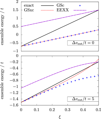
Figure 1: (Color online) Exact and approximate $N$-centered ground-state ensemble energies plotted as a function of $\xi$ for $N=2$ and $U/t=5$ in the symmetric (top panel) and asymmetric (bottom panel) Hubbard dimers. Approximate density-functional energies are computed with the exact ensemble density. The approximations in the $N$-centered ensemble xc functional are $\mbox{EEXX:}~{}E^{\{N,\xi\}}_{\rm xc}(n)\approx E^{\{N,\xi\}}_{\rm x}(n)$, $\mbox{GSxc:}~{}E^{\{N,\xi\}}_{\rm xc}(n)\approx E^{\{N,\xi=0\}}_{\rm x}(n)+E^{\{N,\xi=0\}}_{\rm c}(n)$, and $\mbox{GSc:}~{}E^{\{N,\xi\}}_{\rm xc}(n)\approx E^{\{N,\xi\}}_{\rm x}(n)+E^{\{N,\xi=0\}}_{\rm c}(n)$.

III Application to the asymmetric Hubbard dimer

As a proof of concept, we apply in the following $N$-centered ensemble DFT to the asymmetric Hubbard dimer Carrascal et al. (2015, 2016); Deur et al. (2017). Despite its simplicity, the model is nontrivial and has become in recent years a lab for analyzing and understanding failures of DFT or TD-DFT but also for exploring new ideas Li et al. (2018); Carrascal et al. (2018); Deur et al. (2018); Sagredo and Burke (2018). By using such a model we also illustrate the fact that the theory applies not only to exact ab initio Hamiltonians but also to lattice ones, which might be of interest for modeling extended systems. In the Hubbard dimer, the Hamiltonian is simplified as follows [we write operators in second quantization],

$$\hat{T} \rightarrow -t\sum_{\sigma=\uparrow\downarrow}(\hat{c}^{\dagger}_{0\sigma}\hat{c}_{1\sigma}+\hat{c}^{\dagger}_{1\sigma}\hat{c}_{0\sigma}),\hskip 5.69046pt\hat{W}_{\rm ee}\rightarrow U\sum^{1}_{i=0}\hat{n}_{i\uparrow}\hat{n}_{i\downarrow},$$

$$\hat{V}_{\rm ext} \rightarrow \Delta v_{\rm ext}(\hat{n}_{1}-\hat{n}_{0})/2,\hskip 8.5359pt\hat{n}_{i\sigma}=\hat{c}^{\dagger}_{i\sigma}\hat{c}_{i\sigma},$$ (36)

where $\hat{n}_{i}=\sum_{\sigma=\uparrow\downarrow}\hat{n}_{i\sigma}$ is the density operator on site $i$ ($i=0,1$). Note that the external potential reduces to a single number $\Delta v_{\rm ext}$ which controls the asymmetry of the model. The density also reduces to a single number $n=n_{0}$ which is the occupation of site 0 given that $n_{1}=N-n$. In the following, the central number of electrons will be set to $N=2$ so that the convexity condition reads $\xi_{+}\leq(2-\xi_{-})/3$. As shown in Appendix C, the $N$-centered non-interacting kinetic and EEXX energies can be expressed analytically as follows,

$$T_{\rm s}^{\{N,{\bm{\xi}}\}}(n) = -2t\sqrt{(\xi_{+}-1)^{2}-(n-1)^{2}},$$

$$E_{\rm x}^{\{N,\bm{\xi}\}}(n) = \dfrac{U}{2}\left[1+\dfrac{\xi_{+}-\xi_{-}}{2}+\left(1-\dfrac{3\xi_{+}+\xi_{-}}{2}\right)\left(\dfrac{n-1}{\xi_{+}-1}\right)^{2}\right]$$ (37)

$$-E_{\rm H}(n),$$

where the Hartree energy reads $E_{\rm H}(n)=U\left(1+(n-1)^{2}\right)$. On the other hand, the correlation energy can be computed exactly by Lieb maximization (see Ref. Deur et al. (2017) as well as Appendix C). As readily seen from Eq. (III), an $N$-centered ensemble density $n$ is non-interacting $v$-representable if $|n-1|\leq 1-\xi_{+}$. All the calculations have been performed with $t=1$.

In Fig. 1, the total $N$-centered ground-state ensemble energy is plotted as a function of $\xi_{-}=\xi_{+}=\xi$. The exact ensemble energy is linear in $\xi$, as it should. Results obtained with various density-functional approximations are also shown. In the simplest one, referred to as ground-state xc (GSxc), the weight dependence is taken into account in neither the exchange nor the correlation energies. In other words, the “bare” $\xi$-independent $N$-electron ground-state xc functional is employed. On the other hand, both EEXX-only (simply called EEXX) and the approximation referred to as GSc take the weight dependence into account exactly in the exchange energy. They differ only by the density-functional correlation energy taken at $\xi=0$. The accurate parameterization of Carrascal et al. Carrascal et al. (2015, 2016) has been used for computing the latter correlation energy. Note that, as shown in Appendix C, the exact $N$-centered ensemble correlation functional equals zero when $\xi=1/2$, thus making EEXX truly exact for this particular weight. Returning to Fig. 1, we see that, in the symmetric case [top panel], the approximate ensemble energies exhibit the expected linear behavior in $\xi$. This is simply due to the fact that, in this case, the ensemble density equals 1 and therefore, as readily seen from Eq. (III), all energy contributions vary (individually) linearly with the ensemble weight. Moreover, for $n=1$, the exact ensemble exchange energy is $\xi$-independent, since we consider the particular case $\xi_{+}=\xi_{-}$, which explains why GSxc and GSc ensemble energies are on top of each other. We clearly see, when comparing GSc with the exact result, that the correct ensemble energy slope, and therefore the proper description of the fundamental gap, is recovered only when the weight dependence is taken into account in the correlation energy. This becomes even more critical in the asymmetric case [bottom panel of Fig. 1] where approximations in the xc energy induce curvature, thus leading to a weight-dependent fundamental gap, which is of course unphysical.

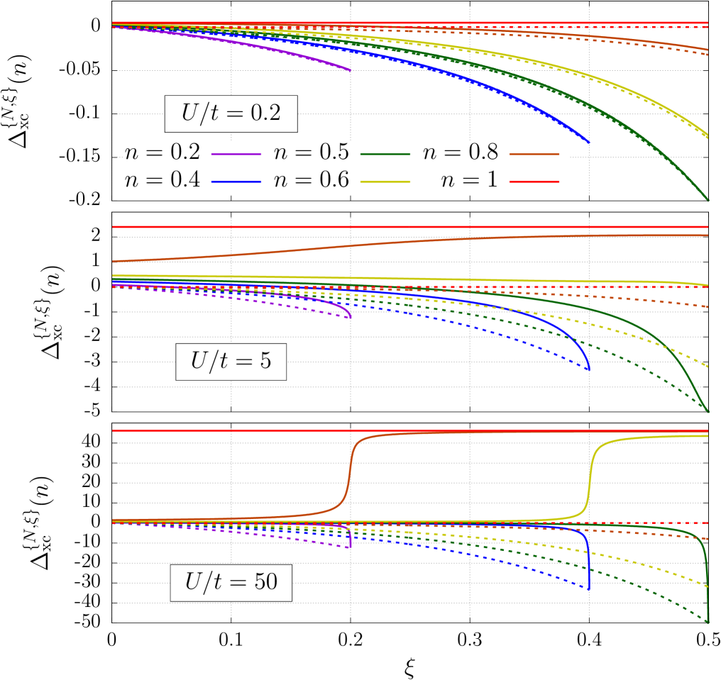
Figure 2: (Color online) Exact GACE integrand plotted as a function of $\xi$ for non-interacting $v$-representable densities [i.e. $|n-1|\leq 1-\xi$, thus leading to $0\leq\xi\leq{\rm inf}\{n,2-n,1/2\}$] and $U/t=0.2$ (top panel), $U/t=5$ (middle panel), and $U/t=50$ (bottom panel). Full lines: xc integrand, dashed lines: exchange-only integrand [see Eq. (92)]. In each panel and for each integrand (xc or x-only), the curves are ordered by decreasing density (the uppermost curve corresponds to $n=1$). See text for further details.

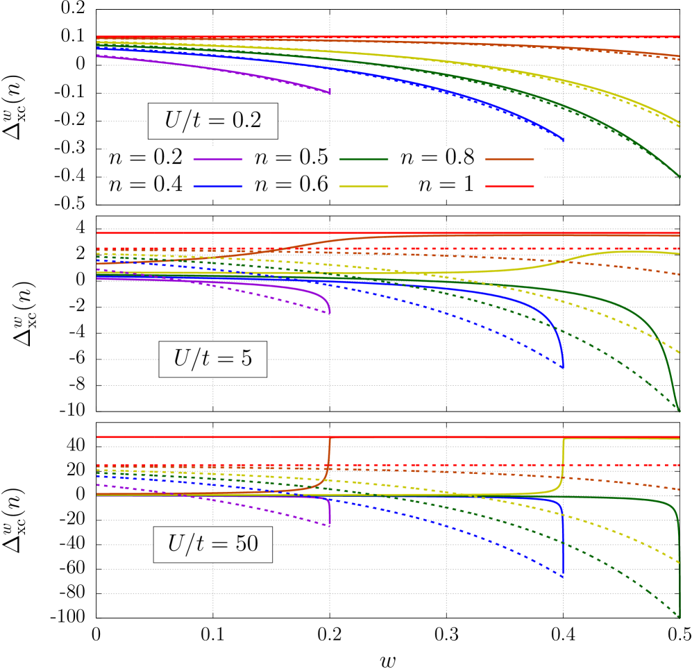
Figure 3: (Color online) Same as Fig. 2 but for the GACE integrand in GOK-DFT where $w$ is the weight assigned to the first (singlet) two-electron excited state. See Ref. Deur et al. (2017) for further details.

More insight into the weight dependence of the ensemble xc energy is given by the GACE integrand in Eq. (11) [see also Appendix C]. As clearly seen when comparing Figs. 2 and 3, even though the integrand differs from its GOK-DFT analog, they both vary similarly with the ensemble weight, in particular in the strongly correlated regime. This can be rationalized by showing, in complete analogy with GOK-DFT (see Sec. 3.3 in Ref. Deur et al. (2018)), that

$$E^{\{N,\xi\}}_{\rm xc}(n)\underset{U/t\rightarrow+\infty}{\longrightarrow}U\times{\rm sup}\big{\{}|1-n|,\xi\big{\}}-E_{\rm H}(n),$$ (38)

which gives (in the $U/t\rightarrow+\infty$ limit) $\partial E^{\{N,\xi\}}_{\rm xc}(n)/\partial\xi=0$ in the non-interacting $v$-representable range $0\leq\xi\leq n$ if $0\leq n\leq 0.5$. For densities in the range $0.5<n\leq 1$, $\partial E^{\{N,\xi\}}_{\rm xc}(n)/\partial\xi=U$ when $0.5\geq\xi>(1-n)$ and $\partial E^{\{N,\xi\}}_{\rm xc}(n)/\partial\xi=0$ when $0\leq\xi<(1-n)$. The same analysis actually holds for the GOK-DFT integrand Deur et al. (2018) (see also Ref. Deur et al. (2017) for further details). Let us finally mention that, in the Lieb maximizations used to produce Figs. 2 and 3, both interacting and non-interacting potentials have been determined numerically. In other words, we computed the expression in Eq. (C.5) rather than the one in Eq. (91) where the analytical expression for the KS potential is used. With such a balanced description of both interacting and non-interacting gaps we do not observe discontinuities in the GACE integrand at $n=\xi$ for densities in the range $0\leq n\leq 0.5$ and large $U/t$ values, unlike in Fig. 6 of Ref. Deur et al. (2017).

Turning to the calculation of the IP, Eq. (35) was verified by calculating each (density-functional) contribution separately (see Appendix C for further details). Results obtained for the asymmetric dimer are shown in Fig. 4.

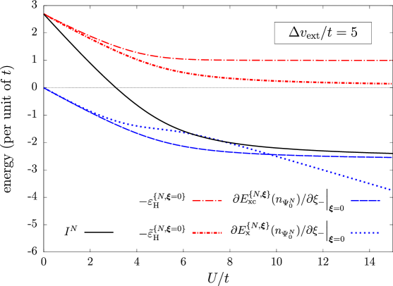
Figure 4: (Color online) Contributions to the exact IP expression in Eq. (35) plotted as a function of $U/t$ for $\Delta v_{\rm ext}/t=5$. The unshifted KS HOMO energy $\varepsilon^{\{N,{\bm{\xi}}=0\}}_{\rm H}$ as well as the exchange-only contribution to the DD are shown for analysis purposes. See text for further details.

As soon as the on-site repulsion is switched on (and up to $U/t\approx 4$), both the shifted KS HOMO energy and the DD (second term in the right-hand side of Eq. (35)) contribute substantially to the IP. Interestingly, in this regime of correlation and density, the shift-in-potential procedure is not crucial. The unshifted KS HOMO energy, which is the analog for the Hubbard dimer of the HOMO energy in a conventional KS-DFT calculation, varies with $U$ through the density. Note that the situation would be completely different in the symmetric case [not shown] where $I^{N}(\Delta v_{\rm ext}=0)=-t-E_{0}^{N}(\Delta v_{\rm ext}=0)$ and the unshifted KS HOMO energy equals $-t$. By construction, the latter energy becomes $\frac{1}{2}E_{0}^{N}(\Delta v_{\rm ext}=0)$ [which is $U$-dependent] after shifting. As a result, in the symmetric case, the shift and the DD equally contribute [by $-(\frac{1}{2}E_{0}^{N}(\Delta v_{\rm ext}=0)+t)$] to the IP. Let us stress that, unlike the shifted KS orbital energies, the unshifted ones are not uniquely defined. They are defined up to a constant, like the KS potential, simply because the density always integrates to a fixed integral number of electrons in $N$-centered ensemble DFT, exactly like in a conventional $N$-electron KS-DFT calculation. The shift will fix the KS orbital energy levels according to Eq. (24), which is equivalent to the Levy–Zahariev shift-in-potential procedure Levy and Zahariev (2014) when ${\bm{\xi}}=0$. In the Hubbard dimer, our value of the unshifted KS HOMO energy has been fixed by choosing a potential whose values on site 0 and 1 sum up to zero [see the potential operator expression in Eq. (III)]. To conclude, as mentioned previously, shifting the KS orbital energies might be, in some cases, as important as taking into account the DD in the calculation of the IP. Returning to Fig. 4, the IP reduces to the xc DD in the strongly correlated regime ($U/t\geq 10$) or, equivalently, the shifted KS HOMO energy becomes negligible. Note that, as expected, taking into account the exchange contribution to the DD only leads to a poor description of the IP when $U/t$ becomes large, thus illustrating the importance of weight dependence in both exchange and correlation energies.

IV Conclusions and perspectives

We have shown that the fundamental gap problem, which is traditionally formulated in grand canonical ensemble DFT, can be recast into a canonical problem where the xc functional becomes ensemble weight dependent. As a remarkable result, modeling the infamous DD becomes equivalent to modeling the weight dependence, exactly like in the optical gap problem. This key result, which is depicted in Eq. (15), opens up a new paradigm in the development of density functional approximations for gaps which are computationally much cheaper than conventional time-dependent post-DFT treatments. A natural step forward would be to apply the approach, for example, to a finite uniform electron gas Loos and Gill (2009), thus providing an ab initio local density-functional approximation that incorporates DDs through its weight dependence. Work is currently in progress in this direction.

Appendix A Connection between the non-interacting kinetic energy functional in GOK-DFT and its analog in $N$-centered ensemble DFT.

For the sake of generality, we will first consider the generalized (interacting) two-weight formulation of the theory [which is introduced in Sec. II.2] and denote $E_{0}^{{\{N,{\bm{\xi}}\}}}[v]$ the $N$-centered ground-state ensemble energy of $\hat{T}+\hat{W}_{\rm ee}+\int{d}\mathbf{r}\;v(\mathbf{r})\hat{n}(\mathbf{r})$. According to the variational principle in Eq. (5), the following inequality holds for any $N$-electron density $n$ and potential $v$,

$$E_{0}^{{\{N,{\bm{\xi}}\}}}[v]\leq F^{{\{N,{\bm{\xi}}\}}}[n]+\int{d}{\mathbf{r}}\,v(\mathbf{r})n(\mathbf{r}),$$ (39)

or, equivalently,

$$F^{{\{N,{\bm{\xi}}\}}}[n]\geq E_{0}^{{\{N,{\bm{\xi}}\}}}[v]-\int{d}{\mathbf{r}}\,v(\mathbf{r})n(\mathbf{r}),$$ (40)

thus leading to the Legendre-Fenchel transform-based expression,

$$F^{{\{N,{\bm{\xi}}\}}}[n]=\sup_{v}\Big{\{}E_{0}^{{\{N,{\bm{\xi}}\}}}[v]-\int{d}{\mathbf{r}}\,v(\mathbf{r})n(\mathbf{r})\Big{\}}.$$ (41)

In the non-interacting case, Eq. (41) becomes

$$T_{\rm s}^{\{N,{\bm{\xi}}\}}[n]=\sup_{v}\Big{\{}\mathcal{E}_{\rm KS}^{\{N,{\bm{\xi}}\}}[v]-\int{d}\mathbf{r}\,v(\mathbf{r})n(\mathbf{r})\Big{\}},$$ (42)

where $\mathcal{E}_{\rm KS}^{\{N,{\bm{\xi}}\}}[v]$ is the $N$-centered ground-state ensemble energy of $\hat{T}+\int{d}\mathbf{r}\;v(\mathbf{r})\hat{n}(\mathbf{r})$. According to Eq. (17), the latter energy can be expressed as follows in terms of the $v$-dependent orbital energies [i.e. the eigenvalues of $-\frac{1}{2}\nabla_{\bf r}^{2}+v(\mathbf{r})$],

$$\mathcal{E}_{\rm KS}^{\{N,\bm{\xi}\}}[v] = \xi_{-}\sum_{i=1}^{N_{-}}\varepsilon_{i}[v]+\xi_{+}\sum_{i=1}^{N_{+}}\varepsilon_{i}[v]$$ (43)

$$+\left[1-\dfrac{N_{-}\xi_{-}}{N}-\dfrac{N_{+}\xi_{+}}{N}\right]\sum_{i=1}^{N}\varepsilon_{i}[v],$$

or, equivalently,

$$\mathcal{E}_{\rm KS}^{\{N,\bm{\xi}\}}[v] = \left[1+\frac{\xi_{-}-\xi_{+}}{N}\right]\sum^{N-2}_{i=1}\varepsilon_{i}[v]$$ (44)

$$+\left[1+\frac{\xi_{-}-\xi_{+}}{N}\right]\varepsilon_{N_{-}}[v]$$

$$+\left[1-\dfrac{N_{-}\xi_{-}+\xi_{+}}{N}\right]\varepsilon_{\rm H}[v]$$

$$+\xi_{+}\varepsilon_{\rm L}[v],$$

where H and L refer to the HOMO and the LUMO of the $N$-electron KS system.

In GOK-DFT, the non-interacting ensemble kinetic energy functional reads Deur et al. (2017, 2018)

$$T_{\rm s}^{N,w}[n]=\sup_{v}\Big{\{}\mathcal{E}_{\rm KS}^{N,w}[v]-\int{d}\mathbf{r}v(\mathbf{r})n(\mathbf{r})\Big{\}},$$ (45)

where the ensemble energy is obtained by averaging the $N$-electron ground- and first-excited-state energies of $\hat{T}+\int{d}\mathbf{r}\;v(\mathbf{r})\hat{n}(\mathbf{r})$ [$w$ is the weight assigned to the excited state],

$$\mathcal{E}_{\rm KS}^{N,w}[v] = (1-w)\sum_{i=1}^{N}\varepsilon_{i}[v]+w\left(\sum_{i=1}^{N_{-}}\varepsilon_{i}[v]+\varepsilon_{\rm L}[v]\right)$$ (46)

$$= \sum_{i=1}^{N_{-}}\varepsilon_{i}[v]+(1-w)\varepsilon_{\rm H}[v]+w\varepsilon_{\rm L}[v].$$

As readily seen from Eqs. (44) and  (46), in the particular case ${\bm{\xi}}=\underline{\xi}\equiv(\xi,\xi)$ [i.e. $\xi_{-}=\xi_{+}=\xi$], we have

$$\mathcal{E}_{\rm KS}^{\{N,\underline{\xi}\}}[v]=\mathcal{E}_{\rm KS}^{N,w=\xi}[v],$$ (47)

thus leading, according to Eqs. (42) and (45), to the equality

$$T_{\rm s}^{\{N,\xi\}}[n]:=T_{\rm s}^{\{N,\underline{\xi}\}}[n]=T_{\rm s}^{N,w=\xi}[n].$$ (48)

Returning to the general (two-weight) expression in Eq. (44), we note that, in the particular case $N=2$, the first term in the right-hand side vanishes. Moreover, since $\varepsilon_{1}[v]=\varepsilon_{2}[v]=\varepsilon_{\rm H}[v]$ within the conventional spin-restricted formalism, it comes

$$\mathcal{E}_{\rm KS}^{\{N=2,\bm{\xi}\}}[v] = (2-\xi_{+})\varepsilon_{\rm H}[v]+\xi_{+}\varepsilon_{\rm L}[v]$$ (49)

$$= \mathcal{E}_{\rm KS}^{N=2,w=\xi_{+}}[v],$$

thus leading to the equality

$$T_{\rm s}^{\{N=2,{\bm{\xi}}\}}[n]=T_{\rm s}^{N=2,w=\xi_{+}}[n].$$ (50)

Appendix B Exact expression for the one-weight GACE integrand in $N$-centered ensemble DFT

According to Eq. (10), the GACE integrand reads

$$\Delta_{\rm xc}^{\{N,\alpha\}}[n]=\dfrac{\partial E_{\rm xc}^{\{N,\alpha\}}[n]}{\partial\alpha},$$ (51)

or, equivalently [see Eqs. (7) and (9)],

$$\Delta_{\rm xc}^{\{N,\alpha\}}[n]=\dfrac{\partial F^{\{N,\alpha\}}[n]}{\partial\alpha}-\dfrac{\partial T_{\rm s}^{\{N,\alpha\}}[n]}{\partial\alpha},$$ (52)

where, with the notations used in Appendix A, $F^{\{N,\alpha\}}[n]:=F^{\{N,\underline{\alpha}\}}[n]$, $T_{\rm s}^{\{N,\alpha\}}[n]:=T_{\rm s}^{\{N,\underline{\alpha}\}}[n]$, and $\underline{\alpha}=(\alpha,\alpha)$. If we denote $v^{\{N,\underline{\alpha}\}}[n]$ and $v_{\rm KS}^{\{N,\underline{\alpha}\}}[n]$ the (stationary) maximizing potentials in Eqs. (41) and (42) [where ${\bm{\xi}}=\underline{\alpha}$], respectively, it comes

$$\dfrac{\partial F^{\{N,\alpha\}}[n]}{\partial\alpha} = \left.\dfrac{\partial E_{0}^{{\{N,\underline{\alpha}\}}}[v]}{\partial\alpha}\right|_{v=v^{\{N,\underline{\alpha}\}}[n]}$$ (53)

and

$$\dfrac{\partial T_{\rm s}^{\{N,\alpha\}}[n]}{\partial\alpha}=\left.\dfrac{\partial\mathcal{E}_{\rm KS}^{\{N,\underline{\alpha}\}}[v]}{\partial\alpha}\right|_{v=v_{\rm KS}^{\{N,\underline{\alpha}\}}[n]},$$ (54)

where, according to Eq. (17) with ${\bm{\xi}}=\underline{\alpha}$ [or, equivalently, Eq. (3)],

$$\dfrac{\partial E_{0}^{{\{N,\underline{\alpha}\}}}[v]}{\partial\alpha}=E^{N}_{\rm g}[v]$$ (55)

is the fundamental gap for the interacting $N$-electron system with Hamiltonian $\hat{T}+\hat{W}_{\rm ee}+\int{d}\mathbf{r}\;v(\mathbf{r})\hat{n}(\mathbf{r})$, and

$$\dfrac{\partial\mathcal{E}_{\rm KS}^{\{N,\underline{\alpha}\}}[v]}{\partial\alpha}=\varepsilon_{\rm L}[v]-\varepsilon_{\rm H}[v]$$ (56)

is the HOMO-LUMO gap for the $N$-electron non-interacting system with Hamiltonian $\hat{T}+\int{d}\mathbf{r}\;v(\mathbf{r})\hat{n}(\mathbf{r})$. Let us stress that, when the interacting and non-interacting potentials are equal to $v^{\{N,\underline{\alpha}\}}[n]$ and $v_{\rm KS}^{\{N,\underline{\alpha}\}}[n]$, respectively, both systems have the same $N$-centered ground-state ensemble density with weight $\underline{\alpha}$, namely $n$. We finally recover Eq. (11) by using the following notations,

$$E^{\{N,\alpha\}}_{\rm g}[n] = E^{N}_{\rm g}\left[v^{\{N,\underline{\alpha}\}}[n]\right]$$

$$\varepsilon^{\{N,\alpha\}}_{i}[n] = \varepsilon_{i}\left[v_{\rm KS}^{\{N,\underline{\alpha}\}}[n]\right],\hskip 5.69046pti={\rm H,L}.$$ (57)

Appendix C Technical details about $N$-centered ensemble DFT for the asymmetric Hubbard dimer

In the following the central number of electrons is set to $N=2$.

C.1 Hole-particle symmetry

In this section we explain how the 3-electron ground-state energy of the Hubbard dimer can be trivially obtained from the one-electron one by using hole-particle symmetry. If we apply the following hole-particle transformation to the annihilation operators in Eq. (III),

$$\hat{c}_{0\sigma} \rightarrow \hat{b}_{0\sigma}=\hat{c}^{\dagger}_{0\sigma},$$

$$\hat{c}_{1\sigma} \rightarrow \hat{b}_{1\sigma}=-\hat{c}^{\dagger}_{1\sigma},$$ (58)

then the Hubbard dimer Hamiltonian,

$$\hat{H}(\Delta v)=-t\sum_{\sigma=\uparrow\downarrow}(\hat{c}^{\dagger}_{0\sigma}\hat{c}_{1\sigma}+\hat{c}^{\dagger}_{1\sigma}\hat{c}_{0\sigma})$$

$$+U\sum^{1}_{i=0}\hat{c}_{i\uparrow}^{\dagger}\hat{c}_{i\uparrow}\hat{c}_{i\downarrow}^{\dagger}\hat{c}_{i\downarrow}+\dfrac{\Delta v}{2}\sum_{\sigma=\uparrow\downarrow}\left(\hat{c}_{1\sigma}^{\dagger}\hat{c}_{1\sigma}-\hat{c}_{0\sigma}^{\dagger}\hat{c}_{0\sigma}\right),$$

can be rewritten as follows, according to the anti-commutation rules,

$$\hat{H}(\Delta v)=-t\sum_{\sigma=\uparrow\downarrow}(\hat{b}^{\dagger}_{0\sigma}\hat{b}_{1\sigma}+\hat{b}^{\dagger}_{1\sigma}\hat{b}_{0\sigma})$$

$$+U\sum^{1}_{i=0}\hat{b}_{i\uparrow}\hat{b}^{\dagger}_{i\uparrow}\hat{b}_{i\downarrow}\hat{b}_{i\downarrow}^{\dagger}+\dfrac{\Delta v}{2}\sum_{\sigma=\uparrow\downarrow}\left(\hat{b}_{1\sigma}\hat{b}^{\dagger}_{1\sigma}-\hat{b}_{0\sigma}\hat{b}^{\dagger}_{0\sigma}\right),$$

or, equivalently,

$$\hat{H}(\Delta v)=-t\sum_{\sigma=\uparrow\downarrow}(\hat{b}^{\dagger}_{0\sigma}\hat{b}_{1\sigma}+\hat{b}^{\dagger}_{1\sigma}\hat{b}_{0\sigma})$$

$$+U\sum^{1}_{i=0}\hat{b}^{\dagger}_{i\uparrow}\hat{b}_{i\uparrow}\hat{b}_{i\downarrow}^{\dagger}\hat{b}_{i\downarrow}-\dfrac{\Delta v}{2}\sum_{\sigma=\uparrow\downarrow}\left(\hat{b}^{\dagger}_{1\sigma}\hat{b}_{1\sigma}-\hat{b}^{\dagger}_{0\sigma}\hat{b}_{0\sigma}\right)$$

$$-U\sum^{1}_{i=0}\sum_{\sigma=\uparrow\downarrow}\hat{b}_{i\sigma}^{\dagger}\hat{b}_{i\sigma}+2U.$$ (61)

As readily seen from Eqs. (C.1) and (C.1), the $\mathcal{N}$-electron ground-state energy $E^{\mathcal{N}}_{0}(\Delta v)$ of $\hat{H}(\Delta v)$ is connected to the $(4-\mathcal{N})$-electron ground-state energy of $\hat{H}(-\Delta v)$ as follows,

$$E^{\mathcal{N}}_{0}(\Delta v)=E^{4-\mathcal{N}}_{0}(-\Delta v)+U(\mathcal{N}-2).$$ (62)

In the particular case $\mathcal{N}=3$, we obtain the useful result [let us recall that $N=2$]

$$E^{N_{+}}_{0}(\Delta v)=E^{N_{-}}_{0}(-\Delta v)+U.$$ (63)

C.2 Exact functionals

In the two-site Hubbard model, the Legendre–Fenchel transform in Eq. (41) can be rewritten as follows,

$$F^{\{N,{\bm{\xi}}\}}(n)=\sup_{\Delta v}\Big{\{}E^{\{N,{\bm{\xi}}\}}(\Delta v)-{\Delta v}(1-n)\Big{\}},$$ (64)

by analogy with GOK-DFT Deur et al. (2017). The interacting ensemble energy reads [with $N=2$],

$$E^{\{N,\bm{\xi}\}}(\Delta v) = \xi_{-}E_{0}^{N_{-}}(\Delta v)+\xi_{+}E_{0}^{N_{+}}(\Delta v)$$ (65)

$$+\left[1-\dfrac{\xi_{-}}{2}-\dfrac{3\xi_{+}}{2}\right]E_{0}^{N}(\Delta v),$$

where the one-electron energy is simply the energy of the HOMO for the non-interacting two-electron system Deur et al. (2017),

$$E_{0}^{N_{-}}(\Delta v)=\varepsilon_{\rm H}(\Delta v)=-\sqrt{t^{2}+(\Delta v^{2}/4)},$$ (66)

and, according to Eq. (63), the 3-electron energy equals

$$E_{0}^{N_{+}}(\Delta v)=\varepsilon_{\rm H}(\Delta v)+U.$$ (67)

Therefore, Eq. (64) can be rewritten as follows,

$$F^{\{N,{\bm{\xi}}\}}(n)=\sup_{\Delta v}\Bigg{\{}(\xi_{-}+\xi_{+})\varepsilon_{\rm H}(\Delta v)+\xi_{+}U$$

$$+\left[1-\dfrac{\xi_{-}}{2}-\dfrac{3\xi_{+}}{2}\right]E_{0}^{N}(\Delta v)-{\Delta v}(1-n)\Bigg{\}},$$ (68)

where the two-electron ground-state energy has the following analytical expression Carrascal et al. (2015, 2016),

$$E_{0}^{N}(\Delta v) = \dfrac{4t}{3}\left(u-w\,{\rm sin}\left(\theta+\dfrac{\pi}{6}\right)\right)$$ (69)

with

$$u = U/2t,$$ (70)

$$w = \sqrt{3(1+\nu^{2})+u^{2}},$$ (71)

$$\nu = \Delta v/2t,$$ (72)

and

$${\rm cos}(3\theta)=\left(9(\nu^{2}-1/2)-u^{2}\right)u/w^{3}.$$ (73)

Note that the maximizing potential $\Delta v^{\{N,{\bm{\xi}}\}}(n)$ in Eq. (C.2), which fulfills the following stationarity condition,

$$\dfrac{\partial F^{\{N,{\bm{\xi}}\}}(n)}{\partial n}=\Delta v^{\{N,{\bm{\xi}}\}}(n),$$ (74)

has no simple analytical expression. However, since the potential-functional quantity to be maximized can be expressed analytically, it is straightforward to compute the exact value of $\Delta v^{\{N,{\bm{\xi}}\}}(n)$ for any density $n$, like in GOK-DFT Deur et al. (2017).
The non-interacting $N$-centered ground-state ensemble kinetic energy functional, i.e. the functional obtained from Eq. (C.2) when $U=0$, has a simple analytical expression given in Eq. (III). This is a direct consequence of Eq. (50) and Eq. (57) in Ref. Deur et al. (2017). Note that, by considering Eq. (74) in the particular case $U=0$, we can express the KS potential analytically as follows,

$$\Delta v_{\rm KS}^{\{N,{\bm{\xi}}\}}(n)=\dfrac{2t(n-1)}{\sqrt{(\xi_{+}-1)^{2}-(1-n)^{2}}}.$$ (75)

Turning to the $N$-centered EEXX energy, let us start with the formal expression

$$E_{\rm x}^{\{N,\bm{\xi}\}}(n)=U\left[\left.\dfrac{\partial F^{\{N,\bm{\xi}\}}(n)}{\partial U}\right|_{U=0}\right]-E_{\rm H}(n),$$ (76)

where, according to Eq. (C.2),

$$\left.\dfrac{\partial F^{\{N,\bm{\xi}\}}(n)}{\partial U}\right|_{U=0}=\xi_{+}$$

$$+\left[1-\dfrac{\xi_{-}}{2}-\dfrac{3\xi_{+}}{2}\right]\left.\dfrac{\partial E_{0}^{N}(\Delta v)}{\partial U}\right|_{U=0,\Delta v=\Delta v_{\rm KS}^{\{N,{\bm{\xi}}\}}(n)},$$ (77)

and, according to Eq. (A7) in Ref. Deur et al. (2017),

$$\left.\dfrac{\partial E_{0}^{N}(\Delta v)}{\partial U}\right|_{U=0}=\dfrac{4t^{2}-8\varepsilon^{2}_{\rm H}(\Delta v)}{4t^{2}+(\Delta v)^{2}-12\varepsilon^{2}_{\rm H}(\Delta v)},$$ (78)

or, equivalently [see Eq. (66)],

$$\left.\dfrac{\partial E_{0}^{N}(\Delta v)}{\partial U}\right|_{U=0}=\dfrac{2t^{2}+(\Delta v)^{2}}{4t^{2}+(\Delta v)^{2}}.$$ (79)

Combining Eqs. (75), and (C.2) with Eq. (79) gives

$$\left.\dfrac{\partial F^{\{N,\bm{\xi}\}}(n)}{\partial U}\right|_{U=0}=\xi_{+}$$

$$+\left[1-\dfrac{\xi_{-}}{2}-\dfrac{3\xi_{+}}{2}\right]\times\dfrac{(1-\xi_{+})^{2}+(1-n)^{2}}{2(1-\xi_{+})^{2}},$$ (80)

thus leading to the expression in Eq. (III) for the EEXX functional.

C.3 Correlation energy at the border of the representability domain

Let us consider the one-weight formulation of $N$-centered ensemble DFT (i.e. $\xi_{-}=\xi_{+}=\xi$). We will show in the following that, at the border of the non-interacting $v$-representability domain [i.e. when $n=1\pm(1-\xi)$], the $N$-centered ground-state ensemble correlation energy equals zero. The proof follows closely its analog in GOK-DFT (see Appendix C in Ref. Deur et al. (2018)).

According to Eq. (C.2), the (unique) maximizing potential $\Delta v^{\{N,\xi\}}(n):=\Delta v^{\{N,\underline{\xi}\}}(n)$ with $\underline{\xi}=(\xi,\xi)$ fulfills the following stationarity condition,

$$\left[-\dfrac{\xi\Delta v}{2\sqrt{t^{2}+(\Delta v^{2}/4)}}+(1-2\xi).\dfrac{\partial E_{0}^{N}(\Delta v)}{\partial\Delta v}\right]_{\Delta v=\Delta v^{\{N,\xi\}}(n)}$$

$$=1-n.$$ (81)

Since $E^{N}_{0}(\Delta v)=U-|\Delta v|$ and ${\partial E^{N}_{0}(\Delta v)}/{\partial\Delta v}=-{\Delta v}/{|\Delta v|}$ when $|\Delta v|/t\rightarrow+\infty$ and $|\Delta v|>U$ [see Ref. Deur et al. (2018)], we conclude that the stationarity condition in Eq. (C.3) is fulfilled for $n=1\pm(1-\xi)$ when $|\Delta v|/t\rightarrow+\infty$ and $\Delta v/(n-1)$ is positive. As a result, in this particular case, the Legendre–Fenchel transform in Eq (C.2) can be simplified as follows,

$$-\xi|\Delta v|+\xi U+(1-2\xi).\Big{(}U-|\Delta v|\Big{)}+|\Delta v|.(1-\xi)$$

$$\underset{|\Delta v|\rightarrow+\infty}{\longrightarrow}F^{\{N,\xi\}}\Big{(}1\pm(1-\xi)\Big{)}=(1-\xi)U.$$ (82)

Since, according to Eq. (III), $T^{\{N,\xi\}}_{\rm s}(1\pm(1-\xi))=0,$ and $E_{\rm x}^{\{N,\xi\}}(1\pm(1-\xi))=(1-\xi)U-E_{\rm H}(n)$, we conclude that

$$E_{\rm c}^{\{N,\xi\}}\Big{(}1\pm(1-\xi)\Big{)}=0.$$ (83)

C.4 Correlation energy and potential for the $N$-centered ensemble with $\xi=1/2$

In the particular case $\xi_{-}=\xi_{+}=\xi=1/2$, the Legendre–Fenchel transform in Eq. (C.2) becomes

$$F^{\{N,\xi=1/2\}}(n) = \sup_{\Delta v}\Bigg{\{}\varepsilon_{\rm H}(\Delta v)+\dfrac{U}{2}-\Delta v(1-n)\Bigg{\}}$$ (84)

$$= T_{\rm s}^{\{N,\xi=1/2\}}(n)+\dfrac{U}{2},$$

where we used the fact that $T_{\rm s}^{\{N,\xi=1/2\}}(n)=F^{\{N,\xi=1/2\}}(U=0,n)$. Interestingly, we first notice that the interacting and non-interacting functionals will have the same maximizing potential, thus leading to

$$\Delta v_{\rm Hxc}^{\{N,\xi=1/2\}}(n) = \Delta v_{\rm KS}^{\{N,\xi=1/2\}}(n)-\Delta v^{\{N,\xi=1/2\}}(n)$$ (85)

$$= 0.$$

Since, according to Eqs. (74), (75) and (III),

$$\Delta v_{\rm Hx}^{\{N,\xi\}}(n) = -\dfrac{\partial}{\partial n}\left[E_{\rm H}(n)+E_{\rm x}^{\{N,\xi\}}(n)\right]$$ (86)

$$= \dfrac{U(1-2\xi)(1-n)}{(1-\xi)^{2}},$$

we conclude that

$$\Delta v_{\rm c}^{\{N,\xi=1/2\}}(n)=0.$$ (87)

Moreover, since $E_{\rm x}^{\{N,\xi=1/2\}}(n)={U}/{2}-E_{\rm H}(n)$, we finally deduce from Eq. (84) that

$$E_{\rm c}^{\{N,\xi=1/2\}}(n)=0.$$ (88)

C.5 GACE integrand

According to Eqs. (11), (66), and (67), the GACE integrand can be calculated as follows,

$$\Delta_{\rm xc}^{\{N,\xi\}}(n)=U-2E_{0}^{N}\left(\Delta v^{\{N,\xi\}}(n)\right)$$

$$+2\varepsilon_{\rm H}\left(\Delta v^{\{N,\xi\}}(n)\right)+2\varepsilon_{\rm H}\left(\Delta v_{\rm KS}^{\{N,\xi\}}(n)\right),$$ (89)

where $\Delta v^{\{N,\xi\}}(n):=\Delta v^{\{N,\underline{\xi}\}}(n)$ [we denote $\underline{\xi}=(\xi,\xi)$] is obtained numerically by Lieb maximization (see Eq. (C.2)) and, according to Eq. (75),

$$\Delta v_{\rm KS}^{\{N,\xi\}}(n)=\dfrac{2t(n-1)}{\sqrt{(\xi-1)^{2}-(1-n)^{2}}}.$$ (90)

We finally obtain from Eq. (66) the simplified expression

$$\Delta_{\rm xc}^{\{N,\xi\}}(n) = U-2E_{0}^{N}\left(\Delta v^{\{N,\xi\}}(n)\right)$$ (91)

$$-\sqrt{4t^{2}+\left[\Delta v^{\{N,{\xi}\}}(n)\right]^{2}}$$

$$-2t\dfrac{(1-\xi)}{\sqrt{(\xi-1)^{2}-(1-n)^{2}}}.$$

The EEXX-only contribution is obtained by differentiating the second line of Eq. (III) [where $\xi_{+}=\xi_{-}=\xi$] with respect to $\xi$, thus leading to

$$\Delta_{\rm x}^{\{N,\xi\}}(n) := \dfrac{\partial E_{\rm x}^{\{N,\underline{\xi}\}}(n)}{\partial\xi}=U\dfrac{\xi(n-1)^{2}}{(\xi-1)^{3}}.$$ (92)

As expected, the latter expression gives a good approximation to the xc GACE integrand in the weakly-correlated regime (see the top panel of Fig. 2). Note also that, for a given density $n$ and any value of $U/t$, the correlation GACE integrand becomes zero when approaching the border of the non-interacting $v$-representability domain, i.e. when $n\rightarrow 1\pm(1-\xi)$ or, equivalently, $\xi\rightarrow 1\pm(1-n)$. This can be related to Eq. (83) which, after differentiation with respect to $\xi$ [note that the infinitesimal variation $\xi\rightarrow\xi-\eta$ where $\eta\rightarrow 0^{+}$ should be considered in order to differentiate the functional within the representability domain], gives

$$\Delta_{\rm c}^{\{N,\xi\}}\Big{(}1\pm(1-\xi)\Big{)}=\left.\dfrac{\partial E_{\rm c}^{\{N,\xi\}}(n)}{\partial\xi}\right|_{n=1\pm(1-\xi)}$$

$$=\pm\left.\dfrac{\partial E_{\rm c}^{\{N,\xi\}}(n)}{\partial n}\right|_{n=1\pm(1-\xi)}$$

$$=\mp\Delta v_{\rm c}^{\{N,\xi\}}\Big{(}1\pm(1-\xi)\Big{)}.$$ (93)

According to Eq. (87), the latter quantity is indeed equal to zero when $\xi=1/2$. Numerical values of the correlation potential obtained by Lieb maximization confirm that this statement holds for $\xi<1/2$, which is in complete agreement with all panels in Fig. 2.

C.6 IP from the shifted HOMO energy and the DD

In order to compute each contribution to the IP expression in Eq. (35) separately, the $N$-centered analog of the Levy–Zahariev shift should be calculated first. From Eq. (19) and the second-quantized expression for local potentials in the two-site model (see Eq. (III)), we obtain

$$C^{\{N,{\bm{\xi}}\}}(n)=\dfrac{1}{2}\left[E_{\rm Hxc}^{\{N,{\bm{\xi}}\}}(n)-(1-n)\Delta v_{\rm Hxc}^{\{N,{\bm{\xi}}\}}(n)\right].$$

Turning to the DD, it comes from Eq. (C.2),

$$\dfrac{\partial F^{\{N,{\bm{\xi}}\}}(n)}{\partial\xi_{-}}=\left[\varepsilon_{\rm H}(\Delta v)-\dfrac{1}{2}E_{0}^{N}(\Delta v)\right]_{\Delta v=\Delta v^{\{N,{\bm{\xi}}\}}(n)}.$$ (95)

Since $\partial T_{\rm s}^{\{N,{\bm{\xi}}\}}(n)/\partial\xi_{-}=0$, we conclude that

$$\dfrac{\partial E^{\{N,{\bm{\xi}}\}}_{\rm xc}(n)}{\partial\xi_{-}}=\left[\varepsilon_{\rm H}(\Delta v)-\dfrac{1}{2}E_{0}^{N}(\Delta v)\right]_{\Delta v=\Delta v^{\{N,{\bm{\xi}}\}}(n)}.$$ (96)

Note that, when ${\bm{\xi}}=0$ and $n=n_{\Psi_{0}^{N}}$ [or, equivalently, $\Delta v^{\{N,{\bm{\xi}}=0\}}(n)=\Delta v_{\rm ext}$],

$$\tilde{\varepsilon}_{\rm H}^{\{N,{\bm{\xi}}=0\}}=E_{0}^{N}(\Delta v_{\rm ext})/2,$$ (97)

and

$$E_{0}^{N_{-}}(\Delta v_{\rm ext})=\varepsilon_{\rm H}(\Delta v_{\rm ext}),$$ (98)

so that Eq. (35) is recovered, as expected.

References

- Hohenberg and Kohn (1964) P. Hohenberg and W. Kohn, Phys. Rev. 136, B864 (1964).
- Kohn and Sham (1965) W. Kohn and L. J. Sham, Phys. Rev. 140, A1133 (1965).
- Levy (1995) M. Levy, Phys. Rev. A 52, R4313 (1995).
- Yang et al. (2014) Z.-h. Yang, J. R. Trail, A. Pribram-Jones, K. Burke, R. J. Needs, and C. A. Ullrich, Phys. Rev. A 90, 042501 (2014).
- Perdew and Levy (1983) J. P. Perdew and M. Levy, Phys. Rev. Lett. 51, 1884 (1983).
- Sham and Schlüter (1983) L. J. Sham and M. Schlüter, Phys. Rev. Lett. 51, 1888 (1983).
- Parr and Bartolotti (1983) R. G. Parr and L. J. Bartolotti, J. Phys. Chem. 87, 2810 (1983).
- Godby et al. (1987) R. W. Godby, M. Schlüter, and L. J. Sham, Phys. Rev. B 36, 6497 (1987).
- Godby et al. (1988) R. W. Godby, M. Schlüter, and L. J. Sham, Phys. Rev. B 37, 10159 (1988).
- Nesbet (1997) R. K. Nesbet, Phys. Rev. A 56, 2665 (1997).
- Harbola (1998) M. K. Harbola, Phys. Rev. A 57, 4253 (1998).
- Chan (1999) G. K.-L. Chan, J. Chem. Phys. 110, 4710 (1999).
- Teale et al. (2008) A. M. Teale, F. De Proft, and D. J. Tozer, J. Chem. Phys. 129, 044110 (2008).
- Yang et al. (2012) W. Yang, A. J. Cohen, and P. Mori-Sánchez, J. Chem. Phys. 136, 204111 (2012).
- Gould and Toulouse (2014) T. Gould and J. Toulouse, Phys. Rev. A 90, 050502 (2014).
- Dimitrov et al. (2016) T. Dimitrov, H. Appel, J. I. Fuks, and A. Rubio, New J. Phys. 18, 083004 (2016).
- Benitez and Proetto (2016) A. Benitez and C. R. Proetto, Phys. Rev. A 94, 052506 (2016).
- Hodgson et al. (2017) M. J. P. Hodgson, E. Kraisler, and E. K. U. Gross, arXiv preprint arXiv:1706.00586 (2017).
- Runge and Gross (1984) E. Runge and E. K. U. Gross, Phys. Rev. Lett. 52, 997 (1984).
- Pickett et al. (1998) W. E. Pickett, S. C. Erwin, and E. C. Ethridge, Phys. Rev. B 58, 1201 (1998).
- Kulik et al. (2006) H. J. Kulik, M. Cococcioni, D. A. Scherlis, and N. Marzari, Phys. Rev. Lett. 97, 103001 (2006).
- Kulik and Marzari (2010) H. J. Kulik and N. Marzari, J. Chem. Phys. 133, 114103 (2010).
- Anisimov et al. (1991) V. I. Anisimov, J. Zaanen, and O. K. Andersen, Phys. Rev. B 44, 943 (1991).
- Liechtenstein et al. (1995) A. I. Liechtenstein, V. I. Anisimov, and J. Zaanen, Phys. Rev. B 52, R5467 (1995).
- Cococcioni and de Gironcoli (2005) M. Cococcioni and S. de Gironcoli, Phys. Rev. B 71, 035105 (2005).
- Imamura et al. (2011) Y. Imamura, R. Kobayashi, and H. Nakai, J. Chem. Phys. 134, 124113 (2011).
- Atalla et al. (2016) V. Atalla, I. Y. Zhang, O. T. Hofmann, X. Ren, P. Rinke, and M. Scheffler, Phys. Rev. B 94, 035140 (2016).
- Stein et al. (2010) T. Stein, H. Eisenberg, L. Kronik, and R. Baer, Phys. Rev. Lett. 105, 266802 (2010).
- Stein et al. (2012) T. Stein, J. Autschbach, N. Govind, L. Kronik, and R. Baer, J. Chem. Phys. Lett. 3, 3740 (2012).
- Bruneval (2012) F. Bruneval, J. Chem. Phys. 136, 194107 (2012).
- Bruneval and Marques (2012) F. Bruneval and M. A. Marques, J. Chem. Theory Comput. 9, 324 (2012).
- Jiang (2015) H. Jiang, Int. J. Quantum Chem. 115, 722 (2015).
- Pacchioni (2015) G. Pacchioni, Catal. Lett. 145, 80 (2015).
- Ou and Subotnik (2016) Q. Ou and J. E. Subotnik, J. Phys. Chem. A 120, 4514 (2016).
- Reining (2018) L. Reining, Wiley Interdisciplinary Reviews: Computational Molecular Science 8, e1344 (2018).
- Gross et al. (1988a) E. K. U. Gross, L. N. Oliveira, and W. Kohn, Phys. Rev. A 37, 2805 (1988a).
- Gross et al. (1988b) E. K. U. Gross, L. N. Oliveira, and W. Kohn, Phys. Rev. A 37, 2809 (1988b).
- Oliveira et al. (1988) L. N. Oliveira, E. K. U. Gross, and W. Kohn, Physical Review A 37, 2821 (1988).
- Yang et al. (2017) Z.-h. Yang, A. Pribram-Jones, K. Burke, and C. A. Ullrich, Phys. Rev. Lett. 119, 033003 (2017).
- Gould and Pittalis (2017) T. Gould and S. Pittalis, Phys. Rev. Lett. 119, 243001 (2017).
- Gould et al. (2018) T. Gould, L. Kronik, and S. Pittalis, J. Chem. Phys. 148, 174101 (2018).
- Deur et al. (2017) K. Deur, L. Mazouin, and E. Fromager, Phys. Rev. B 95, 035120 (2017).
- Deur et al. (2018) K. Deur, L. Mazouin, B. Senjean, and E. Fromager, Eur. Phys. J. B 91, 162 (2018).
- Cohen et al. (2008a) A. J. Cohen, P. Mori-Sánchez, and W. Yang, Science 321, 792 (2008a).
- Cohen et al. (2008b) A. J. Cohen, P. Mori-Sánchez, and W. Yang, Phys. Rev. B 77, 115123 (2008b).
- Mori-Sánchez et al. (2008) P. Mori-Sánchez, A. J. Cohen, and W. Yang, Phys. Rev. Lett. 100, 146401 (2008).
- Sai et al. (2011) N. Sai, P. F. Barbara, and K. Leung, Phys. Rev. Lett. 106, 226403 (2011).
- Kronik et al. (2012) L. Kronik, T. Stein, S. Refaely-Abramson, and R. Baer, J. Chem. Theory Comput. 8, 1515 (2012).
- Refaely-Abramson et al. (2012) S. Refaely-Abramson, S. Sharifzadeh, N. Govind, J. Autschbach, J. B. Neaton, R. Baer, and L. Kronik, Phys. Rev. Lett. 109, 226405 (2012).
- Miranda-Quintana and Ayers (2016) R. A. Miranda-Quintana and P. W. Ayers, Phys. Chem. Chem. Phys. 18, 15070 (2016).
- Li et al. (2017) C. Li, J. Lu, and W. Yang, J. Chem. Phys. 146, 214109 (2017).
- Perdew et al. (2017) J. P. Perdew, W. Yang, K. Burke, Z. Yang, E. K. U. Gross, M. Scheffler, G. E. Scuseria, T. M. Henderson, I. Y. Zhang, A. Ruzsinszky, et al., Proc. Natl. Acad. Sci. 114, 2801 (2017).
- Zhou and Ozolins (2017) F. Zhou and V. Ozolins, arXiv preprint arXiv:1710.08973 (2017).
- Zheng et al. (2011) X. Zheng, A. J. Cohen, P. Mori-Sánchez, X. Hu, and W. Yang, Phys. Rev. Lett. 107, 026403 (2011).
- Zheng et al. (2013) X. Zheng, T. Zhou, and W. Yang, J. Chem. Phys. 138, 174105 (2013).
- Li et al. (2015) C. Li, X. Zheng, A. J. Cohen, P. Mori-Sánchez, and W. Yang, Phys. Rev. Lett. 114, 053001 (2015).
- Andrade and Aspuru-Guzik (2011) X. Andrade and A. Aspuru-Guzik, Phys. Rev. Lett. 107, 183002 (2011).
- Görling (2015) A. Görling, Phys. Rev. B 91, 245120 (2015).
- Thierbach et al. (2017) A. Thierbach, C. Neiss, L. Gallandi, N. Marom, T. Körzdörfer, and A. Görling, J. Chem. Theory Comput. 13, 4726 (2017).
- Kraisler and Kronik (2013) E. Kraisler and L. Kronik, Phys. Rev. Lett. 110, 126403 (2013).
- Kraisler and Kronik (2014) E. Kraisler and L. Kronik, J. Chem. Phys. 140, 18A540 (2014).
- Parr and Yang (1984) R. G. Parr and W. Yang, J. Am. Chem. Soc. 106, 4049 (1984).
- Franck and Fromager (2014) O. Franck and E. Fromager, Mol. Phys. 112, 1684 (2014).
- Nagy (1995) A. Nagy, Int. J. Quantum Chem. 56, 225 (1995).
- Levy and Zahariev (2014) M. Levy and F. Zahariev, Phys. Rev. Lett. 113, 113002 (2014).
- Gidopoulos et al. (2002) N. I. Gidopoulos, P. G. Papaconstantinou, and E. K. U. Gross, Phys. Rev. Lett. 88, 033003 (2002).
- Carrascal et al. (2015) D. J. Carrascal, J. Ferrer, J. C. Smith, and K. Burke, J. Phys. Condens. Matter 27, 393001 (2015).
- Carrascal et al. (2016) D. J. Carrascal, J. Ferrer, J. C. Smith, and K. Burke, J. Phys. Condens. Matter. 29, 019501 (2016).
- Li et al. (2018) C. Li, R. Requist, and E. K. U. Gross, J. Chem. Phys. 148, 084110 (2018).
- Carrascal et al. (2018) D. J. Carrascal, J. Ferrer, N. Maitra, and K. Burke, arXiv preprint arXiv:1802.09988 (2018).
- Sagredo and Burke (2018) F. Sagredo and K. Burke, arXiv preprint arXiv:1806.03392 (2018).
- Loos and Gill (2009) P.-F. Loos and P. M. W. Gill, Phys. Rev. Lett. 103, 123008 (2009).