Analysis of Sequential Quadratic Programming
through the Lens of Riemannian Optimization

Abstract

We prove that a “first-order” Sequential Quadratic Programming (SQP) algorithm for equality constrained optimization has local linear convergence with rate $(1-1/\kappa_{R})^{k}$, where $\kappa_{R}$ is the condition number of the Riemannian Hessian, and global convergence with rate $k^{-1/4}$. Our analysis builds on insights from Riemannian optimization – we show that the SQP and Riemannian gradient methods have nearly identical behavior near the constraint manifold, which could be of broader interest for understanding constrained optimization.

1 Introduction

In this paper, we consider the equality-constrained optimization problem

$$\mathop{\rm minimize}_{x\in\mathbb{R}^{n}} ~{}~{}f(x),$$ (1)

$$\mathop{\rm subject~{}to} ~{}~{}x\in{\mathcal{M}}=\{x:F(x)=0\},$$

where we assume $f:\mathbb{R}^{n}\rightarrow\mathbb{R}$ and $F:\mathbb{R}^{n}\rightarrow\mathbb{R}^{m}$ are $C^{2}$ smooth functions with $m\leq n$.

The focus of this paper is on the local and global convergence rate of “first-order” methods for (1): methods that only query $\nabla f(x)$ at each iteration (but can do whatever they want with the constraint), e.g. projected gradient descent. The iteration complexity of first-order unconstrained optimization has been a foundational result in theoretical machine learning [13, 3], and it would be of interest to improve our understanding in the constrained case too.

While numerous “first-order” methods can solve problem (1) [4, 12], we will restrict attention to two types of methods: Riemannian first-order methods and Sequential Quadratic Programming, which we now briefly review. When $\mathcal{M}$ has a manifold structure near $x_{\star}$, one could use Riemannian optimization algorithms [1], whose iterates are maintained on the constraint set $\mathcal{M}$. Classical Riemannian algorithms proceed by computing the Riemannian gradient and then taking a descent step along the geodesics based on this gradient [8, 6]. Later, Riemannian algorithms are simplified by making use of retraction, a mapping from the tangent space to the manifold that can replace the necessity of computing the exact geodesics while still maintaining the same convergence rate. Intuitively, first-order Riemannian methods can be viewed as variants of projected gradient descent that utilize the manifold structure more carefully. Analyses of many such Riemannian algorithms are given in [1, Section 4].

An alternative approach for solving problem (1) is Sequential Quadratic Programming (SQP) [12, Section 18]. Each iteration of SQP solves a quadratic programming problem which minimizes a quadratic approximation of $f$ on the linearized constraint set ${\left\{x:F(x_{k})+\nabla F(x_{k})(x-x_{k})=0\right\}}$. When the quadratic approximation uses the Hessian of the objective function, the SQP is equivalent to Newton method solving nonlinear equations. When the full Hessian is intractable, one can either approximate the Hessian with BFGS-type updates, or just use some raw estimate such as a big PSD matrix [5]. The iterates need not be (and are often not) feasible, which makes SQP particularly appealing when it is intractable to obtain a feasible start or projection onto the constraint set.

1.1 Contribution and related work

In this paper, we consider the following “first-order” SQP algorithm, which sequentially solves the quadratic program

$$x_{k+1}=\operatorname*{arg\,min} ~{}~{}f(x_{k})+\langle\nabla f(x_{k}),x-x_{k}\rangle+\frac{1}{2\eta}\|x-x_{k}\|_{2}^{2}$$ (2)

$$\mathop{\rm subject~{}to} ~{}~{}F(x_{k})+\nabla F(x_{k})(x-x_{k})=0,$$

where $\eta>0$ is the stepsize. Each iterate only requires ${\left\{\nabla f,\nabla F\right\}}$ (hence first-order). This algorithm can be seen as a cheap prototype SQP (compared with BFGS-type) and is more suitable than Riemannian methods when the retraction onto the constrain set is intractable.

We prove that the SQP (2) has local linear convergence with rate $(1-1/\kappa_{R})^{k}$ where $\kappa_{R}$ is the condition number of the Riemannian Hessian at $x_{\star}$ (Theorem 1), and global convergence with rate $k^{-1/4}$ (Theorem 2). Our work differs from the existing literature in the following ways.

1. We provide explicit convergence rates which is lacking in prior work on SQP. Existing local convergence analysis has focused more on the local quadratic convergence of more expensive BFGS-type SQPs [5, 12], whereas global convergence results are mostly asymptotic [5, 14].

2. We observe and make explicit the fact that the SQP iterates stay “quadratically close” to the manifold when initialized near it (though potentially far from $x_{\star}$) – see Figure 1 for an illustration. Such an observation connects first-order SQP to Riemannian gradient methods and allows us to borrow insights from Riemannian optimization to analyze the SQP.

3. We provide new analysis plans for SQP, based on the fact that SQP iterates quickly becomes nearly identical to Riemannian gradient steps once it gets near the constraint set. Our local analysis builds on a new potential function

   $$\|{\mathsf{P}}_{x_{\star}}(x_{k}-x_{\star})\|_{2}^{2}+\sigma\|{\mathsf{P}}_{x_{\star}}^{\perp}(x_{k}-x_{\star})\|_{2}$$

   for some $\sigma>0$ (see Section 2.2 for definition of the projections), as opposed to the traditionally used exact penalty functions. Our global analysis constructs descent lemmas similar to those in Riemannian gradient methods with additional second-order error terms. These results can be of broader interest for understanding constrained optimization.

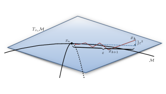
Figure 1: Illustration for SQP iterates

Related work

The convergence rate of many first-order algorithms on problem (1) are shown to achieve local linear convergence with rate $(1-1/\kappa_{R})$, which is termed as the canonical rate in [9]. Riemannian algorithms that achieve the canonical rate include geodesic gradient projection [8, Theorem 2], geodesic steepest descent [6, Theorem 4.4], Riemannian gradient descent [1, Theorem 4.5.6]. The canonical rate is also achieved by the modified Newton method on the quadratic penalty function [9, Section 15.7], which resembles an SQP method in spirit.

Though analyses are well-established for both the Riemannian and the SQP approach (even by the same author in [6] for the Riemannian approach and [7] for the SQP approach), the connection between them did not receive much attention until the past 10 years. Such connection is re-emphasized in [2]: the authors pointed out that the feasibly-projected sequential quadratic programming (FP-SQP) method in [16] gives the same update as the Riemannian Newton update. MS [10] used this connection to provide a framework for selecting a preconditioning metric for Riemannian optimization, in particular when the Riemannian structure is sought on a quotient manifold. However, these connections are established for second-order methods between the Riemannian and the SQP approaches, and such connection for first-order methods are not—we believe—explicitly pointed out yet.

Paper organization

The rest of this paper is organized as the following. In Section 2, we state our assumptions and give preliminaries on the Riemannian geometry on and off the manifold $\mathcal{M}$. We present our local and global convergence result in Section 3.1 and 3.2, and prove them in Section 4 and 5. We give an example in Section 6 and perform numerical experiments in Section 7.

1.2 Notation

For a matrix $A\in\mathbb{R}^{m\times n}$, we denote $A^{\dagger}\in\mathbb{R}^{n\times m}$ as its Moore-Penrose inverse, $A^{\mathsf{T}}\in\mathbb{R}^{n\times m}$ as its transpose, and $A^{\dagger{\mathsf{T}}}$ as the transpose of its Moore-Penrose inverse. As $n\geq m$ and ${\rm rank}(A)=m$, we have $A^{\dagger}=A^{\mathsf{T}}(AA^{\mathsf{T}})^{-1}$. We denote $\sigma_{\min}(A)$ to be the least singular value of matrix $A$. For a $k$’th order tensor $T\in\mathbb{R}^{n_{1}\times n_{2}\times\cdots\times n_{k}}$, and $k$ vectors $u_{1}\in\mathbb{R}^{n_{1}},\ldots,u_{k}\in\mathbb{R}^{n_{k}}$, we denote $T[u_{1},\ldots,u_{k}]=\sum_{i_{1},\ldots,i_{k}}T_{i_{1}\cdots i_{k}}u_{1,i_{1}}\cdots u_{k,i_{k}}$ as tensor-vectors multiplication. The operator norm of tensor $T$ is defined as $\|T\|_{{\rm op}}=\sup_{\|u_{1}\|_{2}=1,\ldots,\|u_{k}\|_{2}=1}T[u_{1},\ldots,u_{k}]$.

For a scaler-valued function $f:\mathbb{R}^{n}\rightarrow\mathbb{R}$, we write its gradient at $x\in\mathbb{R}^{n}$ as a column vector $\nabla f(x)\in\mathbb{R}^{n}$. We write its Hessian at $x\in\mathbb{R}^{n}$ as a matrix $\nabla^{2}f(x)\in\mathbb{R}^{n\times n}$, and its third order derivative at $x$ as a third order tensor $\nabla^{3}f(x)\in\mathbb{R}^{n\times n\times n}$. For a vector-valued function $F:\mathbb{R}^{n}\rightarrow\mathbb{R}^{m}$, its Jacobian matrix at $x\in\mathbb{R}^{n}$ is an $m\times n$ matrix $\nabla F(x)\in\mathbb{R}^{m\times n}$, and its Hessian matrix at $x$ as a third order tensor $\nabla^{2}F(x)\in\mathbb{R}^{m\times n\times n}$.

2 Preliminaries

2.1 Assumptions

Let $x_{\star}$ be a local minimizer of problem (1). Throughout the rest of this paper, we make the following assumptions on problem (1). In particular, all these assumptions are local, meaning that they only depend on the properties of $f$ and $F$ in $\mathsf{B}(x_{\star},\delta)$ for some $\delta>0$.

Assumption 1 (Smoothness).

Within $\mathsf{B}(x_{\star},\delta)$, the functions $f$ and $F$ are $C^{2}$ with local Lipschitz constants ${L_{f}},{L_{F}}$, Lipschitz gradients with constants ${\beta_{f}}$, ${\beta_{F}}$, and Lipschitz Hessians with constants ${\rho_{f}}$, ${\rho_{F}}$.

Assumption 2 (Manifold structure and constraint qualification).

The set $\mathcal{M}$ is a $m$-dimensional smooth submanifold of $\mathbb{R}^{n}$. Further, $\inf_{x\in\mathsf{B}(x_{\star},\delta)}\sigma_{\min}(\nabla F(x))\geq\gamma_{F}$ for some constant $\gamma_{F}>0$.

Smoothness and constraint qualification together implies that the constraints $F(x)$ are well-conditioned and problem (1) is $C^{2}$ near $x_{\star}$. In particular, we can define a matrix ${\rm Hess}f(x_{\star})$ via the formula

$$\quad{\rm Hess}f(x_{\star})={\mathsf{P}}_{x_{\star}}\nabla^{2}f(x_{\star}){\mathsf{P}}_{x_{\star}}-\sum_{i=1}^{m}[\nabla F(x_{\star})^{\dagger{\mathsf{T}}}\nabla f(x_{\star})]_{i}\cdot{\mathsf{P}}_{x_{\star}}\nabla^{2}F_{i}(x_{\star}){\mathsf{P}}_{x_{\star}},$$ (3)

where

$${\mathsf{P}}_{x_{\star}}={\mathsf{I}}_{n}-\nabla F(x_{\star})^{\dagger}\nabla F(x_{\star}).$$ (4)

We can see later that ${\rm Hess}f(x_{\star})$ is the matrix representation of the Riemannian Hessian of function $f$ on ${\mathcal{M}}$ at $x_{\star}$.

Assumption 3 (Eigenvalues of the Riemannian Hessian).

Define

$$\lambda_{\max}=\sup\{\langle u,{\rm Hess}f(x_{\star})u\rangle:\|u\|_{2}=1,\nabla F(x_{\star})u=0\},$$

$$\lambda_{\min}=\inf\{\langle u,{\rm Hess}f(x_{\star})u\rangle:\|u\|_{2}=1,\nabla F(x_{\star})u=0\}.$$

We assume $0<{\lambda_{\min}}\leq{\lambda_{\max}}<\infty$. We call $\kappa_{R}={\lambda_{\max}}/{\lambda_{\min}}$ the condition number of ${\rm Hess}f(x_{\star})$.

2.2 Geometry on the manifold ${\mathcal{M}}$

Since we assumed that the set ${\mathcal{M}}$ is a smooth submanifold of $\mathbb{R}^{n}$, we endow ${\mathcal{M}}$ with the Riemannian geometry induced by the Euclidean space $\mathbb{R}^{n}$. At any point $x\in{\mathcal{M}}$, the tangent space (viewed as a subspace of $\mathbb{R}^{n}$) is obtained by taking the differential of the equality constraints

$$T_{x}{\mathcal{M}}=\{u\in\mathbb{R}^{n}:\nabla F(x)u=0\}.$$ (5)

Let ${\mathsf{P}}_{x}$ be the orthogonal projection operator from $\mathbb{R}^{n}$ onto $T_{x}{\mathcal{M}}$. For any $u\in\mathbb{R}^{n}$, we have

$${\mathsf{P}}_{x}(u) =[{\mathsf{I}}_{n}-\nabla F(x)^{\mathsf{T}}(\nabla F(x)\nabla F(x)^{\mathsf{T}})^{-1}\nabla F(x)]u.$$ (6)

Let ${\mathsf{P}}_{x}^{\perp}$ be the orthogonal projection operator from $\mathbb{R}^{n}$ onto the complement subspace of $T_{x}{\mathcal{M}}$. For any $u\in\mathbb{R}^{n}$, we have

$${\mathsf{P}}_{x}^{\perp}(u) =\nabla F(x)^{\mathsf{T}}(\nabla F(x)\nabla F(x)^{\mathsf{T}})^{-1}\nabla F(x)u.$$ (7)

With a little abuse of notations, we will not distinguish ${\mathsf{P}}_{x}$ and ${\mathsf{P}}_{x}^{\perp}$ with their matrix representations. That is, we also think of ${\mathsf{P}}_{x},{\mathsf{P}}_{x}^{\perp}\in\mathbb{R}^{n\times n}$ as two matrices.

We denote $\nabla f(x)$ and ${\rm grad}f(x)$ respectively the Euclidean gradient and the Riemannian gradient of $f$ at $x\in{\mathcal{M}}$. The Riemannian gradient of $f$ is the projection of the Euclidean gradient onto the tangent space

$${\rm grad}f(x)={\mathsf{P}}_{x}(\nabla f(x))=[{\mathsf{I}}_{n}-\nabla F(x)^{\mathsf{T}}(\nabla F(x)\nabla F(x)^{\mathsf{T}})^{-1}\nabla F(x)]\nabla f(x).$$ (8)

Since $x_{\star}$ is a local minimizer of $f$ on the manifold ${\mathcal{M}}$, we have ${\rm grad}f(x_{\star})=0$.

At $x\in{\mathcal{M}}$, let $\nabla^{2}f(x)$ and ${\rm Hess}f(x)$ be respectively the Euclidean and the Riemannian Hessian of $f$. The Riemannian Hessian is a symmetric operator on the tangent space and is given by projecting the directional derivative of the gradient vector field. That is, for any $u,v\in T_{x}{\mathcal{M}}$, we have (we use ${\mathsf{D}}$ to denote the directional derivative)

$${\rm Hess}f(x)[u,v]=\langle v,{\mathsf{P}}_{x}({\mathsf{D}}{\rm grad}f(x)[u])\rangle$$ (9)

$$= \langle v,{\mathsf{P}}_{x}\cdot\nabla^{2}f(x)u-{\mathsf{P}}_{x}\cdot({\mathsf{D}}{\mathsf{P}}_{x}^{\perp}[u])\cdot\nabla f\rangle$$

$$= v^{\mathsf{T}}{\mathsf{P}}_{x}\nabla^{2}f(x){\mathsf{P}}_{x}u-\nabla^{2}F(x)[\nabla F(x)^{\dagger{\mathsf{T}}}\nabla f(x),u,v].$$

With a little abuse of notation, we will not distinguish the Hessian operator with its matrix representation. That is

$${\rm Hess}f(x)={\mathsf{P}}_{x}\nabla^{2}f(x){\mathsf{P}}_{x}-\sum_{i=1}^{m}[\nabla F(x)^{\dagger{\mathsf{T}}}\nabla f(x)]_{i}\cdot{\mathsf{P}}_{x}\nabla^{2}F_{i}(x){\mathsf{P}}_{x}.$$ (10)

2.3 Geometry off the manifold ${\mathcal{M}}$

We can extend the definition of the matrix representations of the above Riemannian quantities outside the manifold ${\mathcal{M}}$. For any $x\in\mathbb{R}^{n}$, we denote

$$\quad{\mathsf{P}}_{x}={\mathsf{I}}_{n}-\nabla F(x)^{\mathsf{T}}(\nabla F(x)\nabla F(x)^{\mathsf{T}})^{-1}\nabla F(x),$$ (11)

$$\quad{\mathsf{P}}_{x}^{\perp}=\nabla F(x)^{\mathsf{T}}(\nabla F(x)\nabla F(x)^{\mathsf{T}})^{-1}\nabla F(x),$$

$$\quad{\rm grad}f(x)={\mathsf{P}}_{x}\nabla f(x).$$

By the constraint qualification assumption (Assumption 2), $\nabla F(x)\nabla F(x)^{\mathsf{T}}$ is invertible and the quantities above are well defined in $\mathsf{B}(x_{\star},\delta)$. We call ${\rm grad}f(x)$ the extended Riemannian gradient of $f$ at $x$, which extends the Riemannian gradient outside the manifold ${\mathcal{M}}$ as $(f,F)$ are still well-defined there.

2.4 Closed-form expression of the SQP iterate

The above definitions makes it possible to have a concise closed-form expression for the SQP iterate (2). Indeed, as each iterate solves a standard QP, the expression can be obtained explicitly by writing out the optimality condition. Letting $x_{k}=x$, the next iteration $x_{k+1}=x_{+}$ is given by

$$x_{+}=x-\eta[{\mathsf{I}}_{n}-\nabla F(x)^{\mathsf{T}}(\nabla F(x)\nabla F(x)^{\mathsf{T}})^{-1}\nabla F(x)]\nabla f(x)$$ (12)

$$\quad\quad\quad-\nabla F(x)^{\mathsf{T}}(\nabla F(x)\nabla F(x)^{\mathsf{T}})^{-1}F(x)$$

$$=x-\eta{\mathsf{P}}_{x}\nabla f(x)-\nabla F(x)^{\mathsf{T}}(\nabla F(x)\nabla F(x)^{\mathsf{T}})^{-1}F(x)$$

$$=x-\eta{\rm grad}f(x)-\nabla F(x)^{\dagger}F(x).$$

We will frequently refer to this expression in our proof.

3 Main results

3.1 Local convergence theorem

Under Assumptions 1, 2 and 3, we show that the SQP algorithm (2) converges locally linearly with rate $1-1/\kappa_{R}$. The proof can be found in Section 4.

Theorem 1 (Local linear convergence of SQP with canonical rate).

There exists $\varepsilon>0$ and a constant $\sigma>0$ such that the following holds. Let $x_{0}\in\mathsf{B}(x_{\star},\varepsilon)$ and $x_{k}$ be the iterates of Equation (2) with stepsize $\eta=1/\lambda_{\max}({\rm Hess}f(x_{\star}))$. Letting

$$a_{k}= \|{\mathsf{P}}_{x_{\star}}(x_{k}-x_{\star})\|_{2},$$

$$b_{k}= \|{\mathsf{P}}_{x_{\star}}^{\perp}(x_{k}-x_{\star})\|_{2},$$

we have

$$a_{k+1}^{2}+\sigma b_{k+1}\leq\Big{(}1-\frac{1}{2\kappa_{R}}\Big{)}^{2}(a_{k}^{2}+\sigma b_{k}),$$

where $\kappa_{R}=\lambda_{\max}({\rm Hess}f(x_{\star}))/\lambda_{\min}({\rm Hess}f(x_{\star}))$ is the condition number of the Riemannian Hessian of function $f$ on the manifold ${\mathcal{M}}$ at $x_{\star}$. Consequently, the distance $\|x_{k}-x_{\star}\|_{2}^{2}=a_{k}^{2}+b_{k}^{2}$ also converges linearly:

$$\left\|{x_{k}-x_{\star}}\right\|_{2}^{2}\leq O\left((1-1/(2\kappa_{R}))^{k}\right).$$

Remark Theorem 1 requires choosing the stepsize $\eta$ according to the maximum eigenvalue of ${\rm Hess}f(x_{\star})$, which might not be known in advance. In practice, one could implement a line-search (for example as in  [1, Section 4.2] for Riemannian gradient methods) which would hopefully achieve the same optimal rate.

3.2 Global convergence

Let ${\mathcal{M}}_{\varepsilon}=\{x:\|F(x)\|_{2}\leq\varepsilon\}$ denote an $\varepsilon$-neighborhood of the manifold ${\mathcal{M}}$. To show global properties of SQP algorithm, we make the following additional assumptions:

Assumption 4 (Global assumptions).

1. There exists $\varepsilon_{0}\geq 0$, such that $\sup_{x\in{\mathcal{M}}_{\varepsilon_{0}}}\|\nabla f(x)\|_{2}\leq{G_{f}}$, and $\inf_{x\in{\mathcal{M}}_{\varepsilon_{0}}}f(x)\geq{\underline{f}}$.

2. The condition in Assumption 2 holds in this neighborhood ${\mathcal{M}}_{\varepsilon_{0}}$: $\inf_{x\in{\mathcal{M}}_{\varepsilon_{0}}}\sigma_{\min}(\nabla F(x))\geq\gamma_{F}$.

3. Some conditions in Assumption 1 holds globally in $\mathbb{R}^{n}$: the functions $f$ and $F$ are $C^{2}$, $f$ has Lipschitz constant ${L_{f}}$, and $f$ and $F$ have Lipschitz gradients with constants ${\beta_{f}}$, ${\beta_{F}}$.

The following theorem establishes the global convergence of SQP algorithm with a small constant stepsize. Our convergence guarantee is provided in terms of the norm of the extended Riemannian gradient. The proof can be found in Section 5.

Theorem 2.

There exists constants $K_{1},K_{2}>0,\varepsilon_{\star}>0$, such that for any $\varepsilon\leq\varepsilon_{\star}$, we initialize $x_{0}\in{\mathcal{M}}_{\varepsilon}$, and letting step size to be $\eta=\sqrt{\varepsilon/K_{1}}$, then each iterates will be close to the manifold, i.e., $\{x_{i}\}_{i\in\mathbb{N}}\subseteq{\mathcal{M}}_{\varepsilon}$. Moreover, for any $k\in\mathbb{N}$, we have

$$\min_{i\in[k]}\|{\rm grad}f(x_{i})\|_{2}^{2}\leq K_{2}\{[f(x_{0})-{\underline{f}}]/(k\sqrt{\varepsilon})+\sqrt{\varepsilon}\}.$$

To minimize the bound in the right hand side, one can choose $\varepsilon=O(1/k)$, and we get the following corollary.

Corollary 3.1.

There exists constants $\{K_{i}\}_{i=1}^{4}$, such that for any $k\geq K_{1}$, if we take $\varepsilon=K_{2}/k$, and initialize on the manifold ${\mathcal{M}}$ with step size $\eta=K_{3}/k^{1/2}$, we have

$$\min_{i\in[k]}\|{\rm grad}f(x_{i})\|_{2}\leq K_{4}/k^{1/4}.$$

Remark on the stationarity measure While our global convergence is measured the extended Riemannian gradient $\left\|{{\rm grad}f(x_{i})}\right\|_{2}$ on the infeasible iterate $x_{i}$’s, one could construct nearby feasible points with small Riemannian gradient via a straightforward perturbation argument.

4 Proof of Theorem 1

4.1 Riemannian Taylor expansion

The proof of Theorem 1 relies on a particular expansion of the Riemannian gradient off the manifold, which we state as follows.

Lemma 4.1 (First-order expansion of Riemannian gradient).

There exist constants $\varepsilon_{0}>0$ and $C_{r,1},C_{r,2}>0$ such that for all $x\in\mathsf{B}(x_{\star},\varepsilon_{0})$,

$${\rm grad}f(x)={\rm Hess}f(x_{\star})(x-x_{\star})+r(x),$$ (13)

where the remainder term $r(x)$ satisfies the error bound

$$\|r(x)\|_{2}\leq C_{r,1}\|x-x_{\star}\|_{2}^{2}+C_{r,2}\|{\mathsf{P}}_{x_{\star}}^{\perp}(x-x_{\star})\|_{2}.$$ (14)

Lemma 4.1 extends classical Riemannian Taylor expansion [1, Section 7.1] to points off the manifold, where the remainder term contains an additional first-order error. While the error term is linear in $\|{\mathsf{P}}_{x_{\star}}^{\perp}(x-x_{\star})\|_{2}$, this expansion is particularly suitable when $\|{\mathsf{P}}_{x_{\star}}^{\perp}(x-x_{\star})\|_{2}$ is on the order of $\|{\mathsf{P}}_{x_{\star}}(x-x_{\star})\|_{2}^{2}$, which results in a quadratic bound on $\left\|{r(x)}\right\|_{2}$.

In the proof of Theorem 1, ${\rm grad}f(x)$ mostly appears through its squared norm and inner product with $x-x_{\star}$. We summarize the expansion of these terms in the following corollary.

Corollary 4.2.

There exist constants $\varepsilon_{0}>0$ and $C_{r,1},C_{r,2}>0$ such that the following hold. For any $\varepsilon\leq\varepsilon_{0}$, $x\in\mathsf{B}(x,\varepsilon)$,

$$\langle{\rm grad}f(x),x-x_{\star}\rangle=\langle x-x_{\star},{\rm Hess}f(x_{\star})(x-x_{\star})\rangle+R_{1},$$

$$\|{\rm grad}f(x)\|_{2}^{2}=\langle x-x_{\star},[{\rm Hess}f(x_{\star})]^{2}(x-x_{\star})\rangle+R_{2},$$

where

$$\max{\left\{|R_{1}|,|R_{2}|\right\}}\leq\varepsilon(C_{r,1}\|{\mathsf{P}}_{x_{\star}}(x-x_{\star})\|_{2}^{2}+C_{r,2}\|{\mathsf{P}}_{x_{\star}}^{\perp}(x-x_{\star})\|_{2}).$$

4.2 Proof of Theorem 1

The following perturbation bound (see, e.g. [15]) for projections is useful in the proof.

Lemma 4.3.

For $x_{1},x_{2}\in\mathsf{B}(x_{\star},\delta)$, we have

$$\left\|{{\mathsf{P}}_{x_{1}}-{\mathsf{P}}_{x_{2}}}\right\|_{\rm op}\leq{\beta_{P}}\|x_{1}-x_{2}\|_{2}$$

$$\|{\mathsf{P}}_{x_{1}}{\mathsf{P}}_{x_{2}}^{\perp}\|_{{\rm op}}\leq{\beta_{P}}\|x_{1}-x_{2}\|_{2}.$$

where ${\beta_{P}}=2{\beta_{F}}/\gamma_{F}$.

We now prove the main theorem.

Step 1: A trivial bound on $\|x_{+}-x_{\star}\|_{2}^{2}$.

Consider one iterate of the algorithm $x\to x_{+}$, whose closed-form expression is given in (12). We have $x_{+}=x+\Delta$, where

$$\Delta=-\eta\cdot{\rm grad}f(x)-\nabla F(x)^{\dagger}F(x).$$ (15)

We would like to relate $\|x_{+}-x_{\star}\|_{2}$ with $\|x-x_{\star}\|_{2}$. Observe that ${\rm grad}f(x_{\star})=0$, we have

$$\|{\rm grad}f(x)\|_{2}=\|{\rm grad}f(x)-{\rm grad}f(x_{\star})\|_{2}\leq{\beta_{E}}\|x-x_{\star}\|_{2}.$$

Observe that $F(x_{\star})=0$, we have

$$\quad\|\nabla F(x)^{\dagger}F(x)\|_{2}=\|\nabla F(x)^{\dagger}(F(x)-F(x_{\star}))\|_{2}$$

$$\leq\|\nabla F(x)^{\dagger}\|_{{\rm op}}\|F(x)-F(x_{\star})\|_{2}\leq({\beta_{F}}/\gamma_{F})\|x-x_{\star}\|_{2}.$$

Accordingly, we have

$$\quad\|x_{+}-x_{\star}\|_{2}$$

$$\leq\|x-x_{\star}\|_{2}+\eta\|{\rm grad}f(x)\|_{2}+\|\nabla F(x)^{\dagger}F(x)\|_{2}$$

$$\leq[1+\eta{\beta_{E}}+({\beta_{F}}/\gamma_{F})]\|x-x_{\star}\|_{2}.$$

Hence, for any stepsize $\eta$, letting ${C_{d}}=[1+\eta{\beta_{E}}+({\beta_{F}}/\gamma_{F})]^{2}$, for $x\in\mathsf{B}(x_{\star},\delta)$, we have

$$\|x_{+}-x_{\star}\|_{2}^{2}\leq{C_{d}}\|x-x_{\star}\|_{2}^{2}.$$ (16)

Step 2: Analyze normal and tangent distances.

This is the key step of the proof. We look into the normal direction and the tangent direction separately. The intuition for this process is that the normal part of $x-x_{\star}$ is a measure of feasibility, and as we will see, converges much more quickly.

Now we look at equation $x_{+}-x_{\star}=x-x_{\star}+\Delta$. Multiplying it by ${\mathsf{P}}_{x}$ and ${\mathsf{P}}_{x}^{\perp}$ gives

$${\mathsf{P}}_{x}^{\perp}(x_{+}-x_{\star})={\mathsf{P}}_{x}^{\perp}(x-x_{\star})+{\mathsf{P}}_{x}^{\perp}\Delta={\mathsf{P}}_{x}^{\perp}(x-x_{\star})-\nabla F(x)^{\dagger}F(x),$$ (17)

$${\mathsf{P}}_{x}(x_{+}-x_{\star})={\mathsf{P}}_{x}(x-x_{\star})+{\mathsf{P}}_{x}\Delta={\mathsf{P}}_{x}(x-x_{\star})-\eta\cdot{\rm grad}f(x).$$ (18)

We now take squared norms on both equalities and bound the growth. Define the normal and tangent distances as

$$a=\|{\mathsf{P}}_{x_{\star}}(x-x_{\star})\|_{2},~{}~{}~{}b=\|{\mathsf{P}}_{x_{\star}}^{\perp}(x-x_{\star})\|_{2},$$ (19)

and $(a_{+},b_{+})$ similarly for $x_{+}$. Note that the definitions of $a$, $b$ use the projection at $x_{\star}$, so they are slightly different from quantities (17) and (18).

From now on, we assume that $\|x-x_{\star}\|_{2}\leq\varepsilon_{0}$, and $\varepsilon_{0}$ is sufficiently small such that (16) holds. The requirements on $\varepsilon_{0}$ will later be tightened when necessary.

The normal direction.

We have

$$\quad\|{\mathsf{P}}_{x}^{\perp}(x_{+}-x_{\star})\|_{2}^{2}\|{\mathsf{P}}_{x}^{\perp}(x-x_{\star})\|_{2}^{2}+2\langle x-x_{\star},{\mathsf{P}}_{x}^{\perp}\Delta\rangle+\|{\mathsf{P}}_{x}^{\perp}\Delta\|_{2}^{2}$$

$$=\|{\mathsf{P}}_{x}^{\perp}(x-x_{\star})\|_{2}^{2}-2\langle x-x_{\star},\nabla F(x)^{\dagger}F(x)\rangle+\langle F(x),(\nabla F(x)\nabla F(x)^{\mathsf{T}})^{-1}F(x)\rangle$$

$$=\|{\mathsf{P}}_{x}^{\perp}(x-x_{\star})\|_{2}^{2}-2\big{\langle}\nabla F(x)(x-x_{\star}),(\nabla F(x)\nabla F(x)^{\mathsf{T}})^{-1}(\nabla F(x)(x-x_{\star})+r(x))\big{\rangle}$$

$$\quad\quad+\big{\langle}\nabla F(x)(x-x_{\star})+r(x),(\nabla F(x)\nabla F(x)^{\mathsf{T}})^{-1}(\nabla F(x)(x-x_{\star})+r(x))\big{\rangle}$$

$$=\langle r(x),(\nabla F(x)\nabla F(x)^{\mathsf{T}})^{-1}r(x)\rangle,$$

where $r(x)=F(x)-\nabla F(x)(x-x_{\star})$. By the smoothness of function $F$, we have

$$\|r(x)\|_{2}\leq{\beta_{F}}/2\cdot\|x-x_{\star}\|_{2}^{2}.$$

Accordingly, we get

$$\quad\|{\mathsf{P}}_{x}^{\perp}(x_{+}-x_{\star})\|_{2}^{2}$$

$$\leq{\beta_{F}}^{2}/(4\gamma_{F}^{2})\cdot\|x-x_{\star}\|_{2}^{4}={\beta_{F}}^{2}/(4\gamma_{F}^{2})\cdot[\|{\mathsf{P}}_{x_{\star}}^{\perp}(x-x_{\star})\|_{2}^{2}+\|{\mathsf{P}}_{x_{\star}}(x-x_{\star})\|_{2}^{2}]^{2}$$

$$={\beta_{F}}^{2}/(4\gamma_{F}^{2})\cdot(a^{2}+b^{2})^{2}.$$

Applying the perturbation bound on projections (Lemma 4.3), we get

$$\quad b_{+}=\|{\mathsf{P}}_{x_{\star}}^{\perp}(x_{+}-x_{\star})\|_{2}$$ (20)

$$\leq\|{\mathsf{P}}_{x}^{\perp}(x_{+}-x_{\star})\|_{2}+\|{\mathsf{P}}_{x}-{\mathsf{P}}_{x_{\star}}\|_{{\rm op}}\|x_{+}-x_{\star}\|_{2}$$

$$\leq{\beta_{F}}/(2\gamma_{F})\cdot(a^{2}+b^{2})+{\beta_{P}}\|x-x_{\star}\|_{2}\|x_{+}-x_{\star}\|_{2}$$

$$\leq{\beta_{F}}/(2\gamma_{F})\cdot(a^{2}+b^{2})+{\beta_{P}}{C_{d}}\cdot\|x-x_{\star}\|_{2}^{2}$$

$$=\underbrace{[{\beta_{F}}/(2\gamma_{F})+{\beta_{P}}{C_{d}}]}_{{C_{b}}}\cdot(a^{2}+b^{2})={C_{b}}(a^{2}+b^{2}).$$

The tangent direction.

We have

$$\quad\|{\mathsf{P}}_{x}(x_{+}-x_{\star})\|_{2}^{2}$$

$$=\|{\mathsf{P}}_{x}(x-x_{\star})\|_{2}^{2}+2\langle x-x_{\star},{\mathsf{P}}_{x}\Delta\rangle+\|{\mathsf{P}}_{x}\Delta\|_{2}^{2}$$

$$=\|{\mathsf{P}}_{x}(x-x_{\star})\|_{2}^{2}-2\eta\cdot\langle{\rm grad}f(x),x-x_{\star}\rangle+\eta^{2}\cdot\|{\rm grad}f(x)\|_{2}^{2}.$$

Applying Lemma 4.3, we get that for any vector $v$,

$$|\|{\mathsf{P}}_{x}v\|_{2}^{2}-\|{\mathsf{P}}_{x_{\star}}v\|_{2}^{2}|=|\langle v,({\mathsf{P}}_{x_{\star}}-{\mathsf{P}}_{x})v\rangle|\leq{\beta_{P}}\|x-x_{\star}\|_{2}\cdot\|v\|_{2}^{2}.$$

Applying this to vectors $x_{+}-x_{\star}$ and $x-x_{\star}$ gives

$$a_{+}^{2} \leq a^{2}-2\eta\langle{\rm grad}f(x),x-x_{\star}\rangle+\eta^{2}\|{\rm grad}f(x)\|_{2}^{2}$$ (21)

$$\quad+{\beta_{P}}(\|x-x_{\star}\|_{2}^{3}+\|x-x_{\star}\|_{2}\|x_{+}-x_{\star}\|_{2}^{2})$$

$$\leq a^{2}-2\eta\langle{\rm grad}f(x),x-x_{\star}\rangle+\eta^{2}\|{\rm grad}f(x)\|_{2}^{2}$$

$$\quad+{\beta_{P}}(1+{C_{d}})\|x-x_{\star}\|_{2}^{3}.$$

Applying Corollary 4.2, and note that ${\rm Hess}f(x_{\star})={\mathsf{P}}_{x_{\star}}{\rm Hess}f(x_{\star}){\mathsf{P}}_{x_{\star}}$ by the property of the Riemannian Hessian, we get

$$\quad a_{+}^{2}\leq a^{2}-2\eta\langle x-x_{\star},{\rm Hess}f(x_{\star})(x-x_{\star})\rangle+\eta^{2}\langle x-x_{\star},({\rm Hess}f(x_{\star}))^{2}(x-x_{\star})\rangle$$

$$\quad\quad\quad+(-2\eta R_{1}+\eta^{2}R_{2})+\varepsilon_{0}C(a^{2}+b^{2})$$

$$\quad\quad=\langle{\mathsf{P}}_{x_{\star}}(x-x_{\star}),({\mathsf{I}}-\eta{\rm Hess}f(x_{\star}))^{2}{\mathsf{P}}_{x_{\star}}(x-x_{\star})\rangle+(-2\eta R_{1}+\eta^{2}R_{2})+\varepsilon_{0}C(a^{2}+b^{2}),$$

where the remainders are bounded as

$$\max{\left\{|R_{1}|,|R_{2}|\right\}} \leq\varepsilon_{0}\big{(}C_{r,1}\|{\mathsf{P}}_{x_{\star}}(x-x_{\star})\|_{2}^{2}+C_{r,2}\|{\mathsf{P}}_{x_{\star}}^{\perp}(x-x_{\star})\|_{2}\big{)}$$

$$=\varepsilon_{0}(C_{r,1}a^{2}+C_{r,2}b).$$

Choosing the stepsize as $\eta=1/\lambda_{\max}({\rm Hess}f(x_{\star}))$, we have ${\mathsf{I}}-\eta{\rm Hess}f(x_{\star})\preceq(1-1/\kappa_{R}){\mathsf{I}}$. For this choice of $\eta$, using the above bound for $R_{1},R_{2}$, we get that there exists some constant $C_{1},C_{2}$ such that

$$a_{+}^{2}\leq\Big{(}1-\frac{1}{\kappa_{R}}\Big{)}^{2}a^{2}+\varepsilon_{0}(C_{1}a^{2}+C_{2}b).$$ (22)

Putting together.

Let $\sigma>0$ be a constant to be determined. Looking at the quantity $a_{+}^{2}+\sigma b_{+}$, by the bounds (20) and (22) we have

$$\quad a_{+}^{2}+\sigma b_{+}$$

$$\leq\Big{(}1-\frac{1}{\kappa_{R}}\Big{)}^{2}a^{2}+\varepsilon_{0}(C_{1}a^{2}+C_{2}b)+\sigma{C_{b}}(a^{2}+b^{2})$$

$$\leq\Big{(}\Big{(}1-\frac{1}{\kappa_{R}}\Big{)}^{2}+\varepsilon_{0}C_{1}+\sigma{C_{b}}\Big{)}a^{2}+\varepsilon_{0}(C_{2}+\sigma{C_{b}})b.$$

The last inequality is by rearranging the terms and by the assumption that $b=\|{\mathsf{P}}_{x_{\star}}^{\perp}(x-x_{\star})\|_{2}\leq\varepsilon_{0}$. Then, we would like to choose $\sigma$ and $\varepsilon_{0}$ sufficiently small such that

$$\Big{(}1-\frac{1}{\kappa_{R}}\Big{)}^{2}+\varepsilon_{0}C_{1}+\sigma{C_{b}}\leq \Big{(}1-\frac{1}{2\kappa_{R}}\Big{)}^{2},$$ (23)

$$\varepsilon_{0}(C_{2}+\sigma{C_{b}})\leq \sigma.$$ (24)

This can be obtained by first choosing $\sigma$ small to satisfy Eq. (23) leaving a small margin for the choice of $\varepsilon_{0}$, then choosing $\varepsilon_{0}$ small to satisfy both Eq. (23) and (24). With this choice of $\sigma$ and $\varepsilon_{0}$, we have

$$a_{+}^{2}+\sigma b_{+}\leq\Big{(}1-\frac{1}{2\kappa_{R}}\Big{)}^{2}(a^{2}+\sigma b).$$

Step 3: Connect the entire iteration path.

Consider iterates $x_{k}$ of the first-order algorithm (2). Initializing $x^{0}$ sufficiently close to $x_{\star}$, the descent on $a_{k}^{2}+\sigma b_{k}$ ensures $a_{k}^{2}+b_{k}^{2}\leq\varepsilon_{0}^{2}$. Thus we chain this analysis on $(x,x_{+})=(x_{k},x_{k+1})$ and get that $a_{k}^{2}+\sigma b_{k}$ converges linearly with rate $1-1/(2\kappa_{R})$. This in turn implies the bound $a_{k}^{2}+b_{k}^{2}\leq O((1-1/(2\kappa_{R}))^{k})$ by observing that $a_{k}^{2}+b_{k}^{2}\leq C(a_{k}^{2}+\sigma b_{k})$ for some constant $C$.

5 Proof of Theorem 2

The proof of Theorem 2 is directly implied by the following two lemmas. Lemma 5.1 ensures that, as we initialize close to the manifold and choosing step size reasonably small, the iterates will be automatically close to the manifold. Lemma 5.2 shows that, as the iterates are close to the manifold at each step, the value of function $f$ can decrease by a reasonable amount, so that there will be a iterates with small extended Riemannian gradient.

Lemma 5.1.

Let $0<\varepsilon_{1}\leq[\gamma_{F}^{2}/(2{\beta_{F}})]\wedge\varepsilon_{0}$, $x_{0}\in{\mathcal{M}}_{\varepsilon_{1}}$ and $\eta\leq[\varepsilon_{1}/(2{\beta_{F}}{G_{f}}^{2})]^{1/2}$. Then $\{x_{k}\}_{k\geq 0}\subseteq{\mathcal{M}}_{\varepsilon_{1}}$.

Proof    We use proof by induction. We assume $x_{k}\in{\mathcal{M}}_{\varepsilon_{1}}$, i.e., we have $\|F(x_{k})\|_{2}\leq\varepsilon_{1}$. We would like to show that $\|F(x_{k+1})\|_{2}\leq\varepsilon_{1}$, where $x_{k+1}$ gives

$$x_{k+1}=x_{k}-\eta{\rm grad}f(x_{k})-\nabla F(x_{k})^{\dagger}F(x_{k}).$$ (25)

Performing Taylor’s expansion of $F(x_{k+1})$ at $x_{k}$, we have

$$\|F(x_{k+1})\|_{2}=\|F(x_{k}+(x_{k+1}-x_{k}))\|_{2}$$

$$\leq{} \|F(x_{k})-\nabla F(x_{k})[\eta{\rm grad}f(x_{k})+\nabla F(x_{k})^{\dagger}F(x_{k})]\|_{2}+{\beta_{F}}\|x_{k+1}-x_{k}\|_{2}^{2}.$$

Note we have

$$\nabla F(x_{k}){\rm grad}f(x_{k})= \nabla F(x_{k}){\mathsf{P}}_{x_{k}}\nabla f(x_{k})=0,$$

$$\nabla F(x_{k})\nabla F(x_{k})^{\dagger}= {\mathsf{I}}_{n},$$

which gives

$$F(x_{k})-\nabla F(x_{k})[\eta{\rm grad}f(x_{k})+\nabla F(x_{k})^{\dagger}F(x_{k})]=F(x_{k})-F(x_{k})=0.$$

As a result, we have

$$\|F(x_{k+1})\|_{2}={\beta_{F}}\|x_{k+1}-x_{k}\|_{2}^{2}$$

$$= {\beta_{F}}[\eta^{2}\|{\rm grad}f(x_{k})\|_{2}^{2}+F(x_{k})^{\mathsf{T}}\nabla F(x_{k})^{\dagger{\mathsf{T}}}\nabla F(x_{k})^{\dagger}F(x_{k})]$$

$$\leq {\beta_{F}}\eta^{2}{G_{f}}^{2}+({\beta_{F}}/\gamma_{F}^{2})\|F(x_{k})\|_{2}^{2}.$$

Note by induction assumption, we have $\|F(x_{k})\|_{2}\leq\varepsilon_{1}$. Hence as long as $\varepsilon_{1}\leq\gamma_{F}^{2}/(2{\beta_{F}})$ and $\eta^{2}\leq\varepsilon_{1}/(2{\beta_{F}}{G_{f}}^{2})$, we have

$$\|F(x_{k+1})\|_{2}\leq{\beta_{F}}\eta^{2}{G_{f}}^{2}+({\beta_{F}}/\gamma_{F}^{2})\|F(x_{k})\|_{2}^{2}\leq\varepsilon_{1}/2+\varepsilon_{1}/2=\varepsilon_{1}.$$

The lemma holds by noting that the initialization of the induction holds since $x_{0}\in{\mathcal{M}}_{\varepsilon_{1}}$. ∎

Lemma 5.2.

There exists constant $K<\infty$, such that for any $\varepsilon$ satisfying $0<\varepsilon\leq\varepsilon_{\star}=[\gamma_{F}^{2}/(2{\beta_{F}})]\wedge[{\beta_{F}}{G_{f}}^{2}/(2{\beta_{f}}^{2})]\wedge\varepsilon_{0}$, letting $\eta=[\varepsilon/(2{\beta_{F}}{G_{f}}^{2})]^{1/2}$ and initializing $x_{0}\in{\mathcal{M}}_{\varepsilon}$, we have for any $k\in\mathbb{N}$:

$$\min_{i\in[k]}\|{\rm grad}f(x_{i})\|_{2}^{2}\leq K\{[f(x_{0})-{\underline{f}}]/(k\sqrt{\varepsilon})+\sqrt{\varepsilon}\}.$$

Proof    Performing Taylor’s expansion of $f(x_{k+1})$ at $x_{k}$, we have

$$f(x_{k+1})-f(x_{k})-\langle\nabla f(x_{k}),x_{k+1}-x_{k}\rangle\leq{\beta_{f}}\|x_{k+1}-x_{k}\|_{2}^{2}.$$

Using Eq. (25) gives

$$f(x_{k+1})-f(x_{k})+\eta\|{\rm grad}f(x_{k})\|_{2}^{2}+\nabla f(x_{k})^{\mathsf{T}}\nabla F(x_{k})^{\dagger}F(x_{k})$$

$$\leq {\beta_{f}}[\eta^{2}\|{\rm grad}f(x_{k})\|_{2}^{2}+F(x_{k})^{\mathsf{T}}\nabla F(x_{k})^{\dagger{\mathsf{T}}}\nabla F(x_{k})^{\dagger}F(x_{k})]$$

$$\leq {\beta_{f}}[\eta^{2}\|{\rm grad}f(x_{k})\|_{2}^{2}+(1/\gamma_{F}^{2})\|F(x_{k})\|_{2}^{2}].$$

By the choice of $\varepsilon$ and $\eta$, we have $\eta\leq 1/(2{\beta_{f}})$, rearranging the terms gives

$$f(x_{k+1})-f(x_{k})+(\eta/2)\|{\rm grad}f(x_{k})\|_{2}^{2}$$

$$\leq ({L_{f}}/\gamma_{F})\|F(x_{k})\|_{2}+({\beta_{f}}/\gamma_{F}^{2})\|F(x_{k})\|_{2}^{2}$$

$$\leq [({L_{f}}/\gamma_{F})+({\beta_{f}}/\gamma_{F}^{2})\varepsilon_{\star}]\varepsilon\equiv K_{0}\varepsilon.$$

Performing telescope summation and rearranging the terms,

$$\frac{1}{k}\sum_{i=1}^{k}\|{\rm grad}f(x_{i})\|_{2}^{2}\leq 2[f(x_{0})-f(x_{k})]/(k\eta)+2K_{0}\varepsilon/\eta\leq K\{[f(x_{0})-f(x_{k})]/(k\sqrt{\varepsilon})+\sqrt{\varepsilon}\},$$

for some constant $K$. Since we know $x_{k}\in{\mathcal{M}}_{\varepsilon}$, this concludes the proof of this lemma. ∎

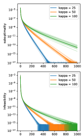
(a) Vary $\kappa$

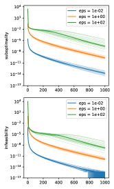
(b) Vary $\varepsilon$

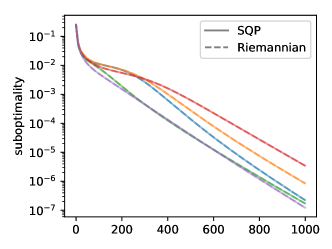
(c) Compare SQP and Riemannian

Figure 2: Convergence of SQP. (a)(b) Effect of condition number and initialization radius on the convergence. Thins lines show all the 20 instances and bold lines indicate the median performance. (c) Comparing SQP and Riemannian gradient descent over 5 instances.

6 Example

We provide the eigenvalue problem as a simple example illustrating our convergence result. We emphasize that this is a simple and well-studied problem; our goal here is only to illustrate the connection between SQP and the Riemannian algorithms.

Example 1 (SQP for eigenvalue problems):  Consider the eigenvalue problem for a symmetric matrix $A\in\mathbb{R}^{n\times n}$:

$$\mathop{\rm minimize} ~{}~{}\frac{1}{2}x^{\top}Ax$$ (26)

$$\mathop{\rm subject~{}to} ~{}~{}\left\|{x}\right\|_{2}^{2}-1=0.$$

This is an instance of problem (1) with $f(x)=(1/2)x^{\top}Ax$ and $F(x)=\left\|{x}\right\|_{2}^{2}-1$. Let $\lambda_{1}<\lambda_{2}\leq\dots\leq\lambda_{n}$ be the eigenvalues of $A$, and $v_{i}(A)$ be the corresponding eigenvectors.

The SQP iterate for this problem is $x\mapsto x_{+}=x+\Delta$, where $\Delta$ solves the subproblem

$$\mathop{\rm minimize} ~{}~{}\langle Ax,\Delta\rangle+\frac{1}{2\eta}\left\|{\Delta}\right\|_{2}^{2}$$

$$\mathop{\rm subject~{}to} ~{}~{}\left\|{x}\right\|_{2}^{2}+2\langle x,\Delta\rangle-1=0.$$

Applying (12), we obtain the explicit formula

$$x_{+}=\frac{\left\|{x}\right\|_{2}^{2}+1}{2\left\|{x}\right\|_{2}^{2}}x-\eta\Big{(}{\mathsf{I}}_{n}-\frac{xx^{\top}}{\left\|{x}\right\|_{2}^{2}}\Big{)}Ax.$$ (27)

By Theorem 1, the local convergence rate is $1-1/\kappa_{R}$, which we now examine. At $x_{\star}=v_{1}(A)$, we have ${\rm Hess}f(x_{\star})=A-\lambda_{1}{\mathsf{I}}_{n}$, and the tangent space $\mathcal{T}_{x_{\star}}\mathcal{M}={\rm span}(v_{2}(A),\dots,v_{n}(A))$. Therefore, the condition number of the Riemannian Hessian is

$$\kappa_{R}=\frac{\sup_{v\in\mathcal{T}_{x_{\star}}\mathcal{M},\left\|{v}\right\|_{2}=1}\langle v,{\rm Hess}f(x_{\star})v\rangle}{\inf_{v\in\mathcal{T}_{x_{\star}}\mathcal{M},\left\|{v}\right\|_{2}=1}\langle v,{\rm Hess}f(x_{\star})v\rangle}=\frac{\lambda_{n}-\lambda_{1}}{\lambda_{2}-\lambda_{1}}.$$

Hence, choosing the right stepsize $\eta$, the convergence rate of the SQP method is

$$1-\frac{1}{\kappa_{R}}=\frac{\lambda_{n}-\lambda_{2}}{\lambda_{n}-\lambda_{1}},$$

matching the rate of power iteration and Riemannian gradient descent.

The keen reader might find that the iterate (27) converges globally to $x_{\star}$ as long as $\langle x_{0},x_{\star}\rangle\neq 0$. This is more optimistic than our Theorem 2 (which only guarantees global convergence to stationary point). Whether such global convergence holds more generally would be an interesting direction for future study. $\Diamond$

7 Numerical experiments

Setup

We experiment with the SQP algorithm on random instances of the eigenvalue problem (26) with $d=1000$. Each instance $A$ was generated randomly with a controlled condition number $\kappa_{R}=\frac{\lambda_{n}-\lambda_{1}}{\lambda_{2}-\lambda_{1}}$, and the stepsize was chosen as $\eta=\frac{1}{2(\lambda_{n}-\lambda_{1})}$ to optimize for the local linear rate. The initialization $x_{0}$ is sampled randomly around the solution $x_{\star}$ with average distance $\varepsilon$ (recall $\left\|{x_{\star}}\right\|_{2}=1$).

We run the following three sets of comparisons and plot the results in Figure 2.

1. Test the effect of $\kappa_{R}$ on the local linear rate, with $\kappa_{R}\in{\left\{25,50,100\right\}}$ and fixed $\varepsilon=0.01$.

2. Test the effect of initialization radius $\varepsilon$ (i.e. localness) on the convergence, with $\varepsilon\in{\left\{0.01,1,100\right\}}$ and fixed $\kappa=100$.

3. Test whether SQP is close to Riemannian gradient descent when initialized at a same feasible start $x_{0}\in\mathcal{M}$.

Results

In experiment (a), we see indeed that the local linear rate of SQP scales as $1-C/\kappa_{R}$: doubling the condition number will double the number of iterations required for halving the sub-optimality. Experiment (b) shows that the linear convergence is indeed more robust locally than globally; when initialized very far away ($\varepsilon=100$), linear convergence with the same rate happens on most of the instances after a while, but there does exist bad instances on which the convergence is slow. This corroborates our theory that the global convergence of SQP is more sensitive to the stepsize choice as the SQP is not guaranteed to approach the manifold when initialized far away. Experiment (c) verifies our intuition that SQP is approximately equal to Riemannian gradient descent: with a feasible start, their iterates stay almost exactly the same.

8 Conclusion

We established local and global convergence of a cheap SQP algorithm building on intuitions from Riemannian optimization. Potential future directions include generalizing our global result to “far from the manifold”, as well as identifying problem structures under which we obtain global convergence to local minimum.

Appendix A Proof of technical results

A.1 Some tools

Lemma A.1 ([11]).

For $x_{1},x_{2}\in\mathsf{B}(x_{\star},\delta)$, we have

$$\|\nabla F(x_{1})^{\dagger}-\nabla F(x_{2})^{\dagger}\|_{{\rm op}}\leq{\beta_{D}}\|x_{1}-x_{2}\|_{2}.$$

where ${\beta_{D}}=2{\beta_{F}}/\gamma_{F}^{2}$.

Lemma A.2.

The extended Riemannian gradient ${\rm grad}f(x)$ is ${\beta_{E}}$-Lipschitz in $\mathsf{B}(x_{\star},\delta)$, where ${\beta_{E}}={\beta_{P}}{L_{f}}+{\beta_{f}}$.

Proof    We have

$$\|{\rm grad}f(x_{1})-{\rm grad}f(x_{2})\|_{2}= \|{\mathsf{P}}_{x_{1}}\nabla f(x_{1})-{\mathsf{P}}_{x_{2}}\nabla f(x_{2})\|_{2}$$

$$\leq \|({\mathsf{P}}_{x_{1}}-{\mathsf{P}}_{x_{2}})\nabla f(x_{1})\|_{2}+\|{\mathsf{P}}_{x_{2}}(\nabla f(x_{1})-\nabla f(x_{2}))\|_{2}$$

$$\leq ({\beta_{P}}{L_{f}}+{\beta_{f}})\|x_{1}-x_{2}\|_{2}.$$

∎

A.2 Proof of Lemma 4.1

For any $x\in\mathsf{B}(x_{\star},\varepsilon_{0})$, denote $x_{p}={\mathsf{P}}_{x_{\star}}(x-x_{\star})+x_{\star}$. We prove the following equation first

$${\rm grad}f(x_{p})={\rm Hess}f(x_{\star})(x_{p}-x_{\star})+r(x_{p}),$$ (28)

where $r(x_{p})\leq C_{r,1}\|x_{p}-x_{\star}\|_{2}^{2}$.

First, we show that ${\rm grad}f(x_{p})$ can be well approximated by ${\mathsf{P}}_{x_{\star}}{\rm grad}f(x_{p})$. Denoting $r_{0}={\mathsf{P}}_{x_{\star}}{\rm grad}f(x_{p})-{\rm grad}f(x_{p})$, by Lemma 4.3 and A.2, we have

$$\|r_{0}\|_{2}= \|{\mathsf{P}}_{x_{\star}}^{\perp}{\rm grad}f(x_{p})\|_{2}=\|{\mathsf{P}}_{x_{\star}}^{\perp}{\mathsf{P}}_{x_{p}}{\rm grad}f(x_{p})\|_{2}$$

$$\leq \|{\mathsf{P}}_{x_{\star}}^{\perp}{\mathsf{P}}_{x_{p}}\|_{{\rm op}}\cdot\|{\rm grad}f(x_{p})\|_{2}\leq{\beta_{P}}\|x_{p}-x_{\star}\|_{2}\|{\rm grad}f(x_{p})\|_{2}\leq{\beta_{P}}{\beta_{E}}\|x_{p}-x_{\star}\|_{2}^{2}.$$

Then, for any $u\in\mathbb{R}^{n}$ with $\|u\|_{2}=1$, we have

$$\langle u,{\mathsf{P}}_{x_{\star}}{\rm grad}f(x_{p})\rangle$$

$$= \langle u,{\mathsf{P}}_{x_{\star}}{\mathsf{P}}_{x_{p}}\{\nabla f(x_{\star})+\nabla^{2}f(x_{\star})(x_{p}-x_{\star})+1/2\cdot\nabla^{3}f(\tilde{x}_{p})[\,\cdot\,,(x_{p}-x_{\star})^{\otimes 2}]\}\rangle$$

$$= \langle u,{\mathsf{P}}_{x_{\star}}{\mathsf{P}}_{x_{p}}[\nabla f(x_{\star})+\nabla^{2}f(x_{\star})(x_{p}-x_{\star})]\rangle+r_{1},$$

where

$$|r_{1}|=1/2\cdot|\langle u,{\mathsf{P}}_{x_{\star}}{\mathsf{P}}_{x_{p}}\nabla^{3}f(\tilde{x}_{p})[\,\cdot\,,(x_{p}-x_{\star})^{\otimes 2}]\rangle\leq 1/2\cdot{\rho_{f}}\|x_{p}-x_{\star}\|_{2}^{2}.$$

Then we have

$$\langle u,{\mathsf{P}}_{x_{\star}}{\rm grad}f(x_{p})\rangle$$

$$= \langle u,{\mathsf{P}}_{x_{\star}}{\mathsf{P}}_{x_{p}}[\nabla f(x_{\star})+\nabla^{2}f(x_{\star})(x_{p}-x_{\star})]\rangle+r_{1},$$

$$= \langle u,{\mathsf{P}}_{x_{\star}}{\mathsf{P}}_{x_{p}}\nabla f(x_{\star})\rangle+\langle u,{\mathsf{P}}_{x_{\star}}\nabla^{2}f(x_{\star})(x_{p}-x_{\star})\rangle+\langle u,{\mathsf{P}}_{x_{\star}}({\mathsf{P}}_{x_{p}}-{\mathsf{P}}_{x_{\star}})\nabla^{2}f(x_{\star})(x_{p}-x_{\star})\rangle+r_{1}$$

$$= \underbrace{\langle u,{\mathsf{P}}_{x_{\star}}{\mathsf{P}}_{x_{p}}\nabla f(x_{\star})\rangle}_{\rm I}+\langle u,{\mathsf{P}}_{x_{\star}}\nabla^{2}f(x_{\star})(x_{p}-x_{\star})\rangle+r_{1}+r_{2},$$

where

$$|r_{2}|=|\langle u,{\mathsf{P}}_{x_{\star}}({\mathsf{P}}_{x_{p}}-{\mathsf{P}}_{x_{\star}})\nabla^{2}f(x_{\star})(x_{p}-x_{\star})\rangle|\leq{\beta_{P}}{\beta_{f}}\|x_{p}-x_{\star}\|_{2}^{2}.$$

Then we look at the term $\rm I$. We have

$$\rm I= -\langle u,{\mathsf{P}}_{x_{\star}}\nabla F(x_{p})^{\mathsf{T}}\nabla F(x_{p})^{\dagger{\mathsf{T}}}\nabla f(x_{\star})\rangle$$

$$= -\langle u,{\mathsf{P}}_{x_{\star}}[\nabla F(x_{p})-\nabla F(x_{\star})]^{\mathsf{T}}\nabla F(x_{p})^{\dagger{\mathsf{T}}}\nabla f(x_{\star})\rangle$$

$$= -\langle u,{\mathsf{P}}_{x_{\star}}\{\nabla^{2}F(x_{\star})[\,\cdot\,,\,\cdot\,,x_{p}-x_{\star}]+1/2\cdot\nabla^{3}F(\tilde{x}_{p})[\,\cdot\,,\,\cdot\,,(x_{p}-x_{\star})^{\otimes 2}]\}^{\mathsf{T}}\nabla F(x_{p})^{\dagger{\mathsf{T}}}\nabla f(x_{\star})\rangle$$

$$= -\sum_{i=1}^{m}[\nabla F(x_{p})^{\dagger{\mathsf{T}}}\nabla f(x_{\star})]_{i}\nabla^{2}F_{i}(x_{\star})[x_{p}-x_{\star},{\mathsf{P}}_{x_{\star}}u]+r_{3},$$

where

$$|r_{3}|= 1/2\cdot|\sum_{i=1}^{m}[\nabla F(x_{p})^{\dagger{\mathsf{T}}}\nabla f(x_{\star})]_{i}\nabla^{3}F_{i}(\tilde{x}_{p})[(x_{p}-x_{\star})^{\otimes 2},{\mathsf{P}}_{x_{\star}}u]|$$

$$\leq {\rho_{F}}{L_{f}}/(2\gamma_{F})\cdot\|x_{p}-x_{\star}\|_{2}^{2}.$$

We further have

$$\rm I= -\sum_{i=1}^{m}[\nabla F(x_{p})^{\dagger{\mathsf{T}}}\nabla f(x_{\star})]_{i}\nabla^{2}F_{i}(x_{\star})[x_{p}-x_{\star},{\mathsf{P}}_{x_{\star}}u]+r_{3}$$

$$= -\sum_{i=1}^{m}[\nabla F(x_{\star})^{\dagger{\mathsf{T}}}\nabla f(x_{\star})]_{i}\nabla^{2}F_{i}(x_{\star})[x_{p}-x_{\star},{\mathsf{P}}_{x_{\star}}u]+r_{3}+r_{4},$$

where

$$|r_{4}|=\sum_{i=1}^{m}\{[\nabla F(x_{p})-\nabla F(x_{\star})]^{\dagger{\mathsf{T}}}\nabla f(x_{\star})\}_{i}\nabla^{2}F_{i}(x_{\star})[x_{p}-x_{\star},P_{x_{\star}}u]\leq{\beta_{D}}{L_{f}}{\beta_{F}}\cdot\|x_{p}-x_{\star}\|_{2}^{2}.$$

Above all, combining all the terms, we have

$$|\langle u,{\rm grad}f(x_{p})-{\rm Hess}f(x_{p})(x_{p}-x_{\star})\rangle|\leq\|r_{0}\|_{2}+|r_{1}+r_{2}+r_{3}+r_{4}|$$

$$\leq ({\beta_{P}}{\beta_{E}}+1/2\cdot{\rho_{f}}+{\beta_{P}}{\beta_{f}}+{\rho_{F}}{L_{f}}/(2\gamma_{F})+{\beta_{D}}{L_{f}}{\beta_{F}})\|x_{p}-x_{\star}\|_{2}^{2}.$$

Taking $C_{r,1}={\beta_{P}}{\beta_{E}}+1/2\cdot{\rho_{f}}+{\beta_{P}}{\beta_{f}}+{\rho_{F}}{L_{f}}/(2\gamma_{F})+{\beta_{D}}{L_{f}}{\beta_{F}}$ we get Eq. (28).

Then by Lemma A.2, we have

$$\|{\rm grad}f(x)-{\rm grad}f(x_{p})\|\leq C_{r,2}\|x-x_{p}\|_{2}.$$ (29)

This proves the lemma.

A.3 Proof of Corollary 4.2

Let $\varepsilon_{0}$ be given by Lemma 4.1, $\varepsilon\leq\varepsilon_{0}$, and $x\in\mathsf{B}(x,\varepsilon)$. We have

$${\rm grad}f(x)={\rm Hess}f(x_{\star})(x-x_{\star})+r(x),~{}~{}\|r(x)\|_{2}\leq C_{r,1}\|x-x_{\star}\|_{2}^{2}+C_{r,2}\|{\mathsf{P}}_{x_{\star}}^{\perp}(x-x_{\star})\|_{2}.$$ (30)

Therefore we obtain the expansion

$$\langle{\rm grad}f(x),x-x_{\star}\rangle=\langle x-x_{\star},{\rm Hess}f(x_{\star})(x-x_{\star})\rangle+R_{1},$$

where $R_{1}$ is bounded as

$$\quad|R_{1}|=|\langle r(x),x-x_{\star}\rangle|\leq C_{r,1}\|x-x_{\star}\|_{2}^{3}+C_{r,2}\|x-x_{\star}\|_{2}\|{\mathsf{P}}_{x_{\star}}^{\perp}(x-x_{\star})\|_{2}$$ (31)

$$\leq\varepsilon C_{r,1}\|x-x_{\star}\|_{2}^{2}+\varepsilon C_{r,2}\|{\mathsf{P}}_{x_{\star}}^{\perp}(x-x_{\star})\|_{2}.$$

Similarly, we have the expansion

$$\|{\rm grad}f(x_{\star})\|_{2}^{2}=\langle x-x_{\star},({\rm Hess}f(x_{\star}))^{2}(x-x_{\star})\rangle+R_{2},$$

where $R_{2}$ is bounded as (letting $H=\lambda_{\max}({\rm Hess}f(x_{\star}))$ for convenience)

$$\quad|R_{2}|\leq 2|\langle{\rm Hess}f(x_{\star})(x-x_{\star}),r(x)\rangle|+\|r(x)\|_{2}^{2}$$ (32)

$$\leq 2H\big{(}C_{r,1}\|x-x_{\star}\|_{2}^{3}+C_{r,2}\|x-x_{\star}\|_{2}\|{\mathsf{P}}_{x_{\star}}^{\perp}(x-x_{\star})\|_{2}\big{)}$$

$$\quad+\big{(}C_{r,1}^{2}\|x-x_{\star}\|_{2}^{4}+2C_{r,1}C_{r,2}\|x-x_{\star}\|_{2}^{2}\|{\mathsf{P}}_{x_{\star}}^{\perp}(x-x_{\star})\|_{2}+C_{r,2}^{2}\|{\mathsf{P}}_{x_{\star}}^{\perp}(x-x_{\star})\|_{2}^{2}\big{)}$$

$$\leq(2HC_{r,1}\varepsilon+C_{r,1}^{2}\varepsilon^{2})\|x-x_{\star}\|_{2}^{2}+(2HC_{r,2}\varepsilon+2C_{r,1}C_{r,2}\varepsilon^{2})\|{\mathsf{P}}_{x_{\star}}^{\perp}(x-x_{\star})\|_{2}+C_{r,2}^{2}\varepsilon\|{\mathsf{P}}_{x_{\star}}^{\perp}(x-x_{\star})\|_{2}$$

$$\leq\varepsilon\underbrace{(2HC_{r,1}+C_{r,1}^{2}\varepsilon_{0})}_{\widetilde{C}_{r,1}}\|x-x_{\star}\|_{2}^{2}+\varepsilon\underbrace{(2HC_{r,2}+2C_{r,1}C_{r,2}\varepsilon_{0}+C_{r,2}^{2}\varepsilon_{0})}_{\widetilde{C}_{r,2}}\|{\mathsf{P}}_{x_{\star}}^{\perp}(x-x_{\star})\|_{2}$$

$$=\varepsilon\big{(}\widetilde{C}_{r,1}\|x-x_{\star}\|_{2}^{2}+\widetilde{C}_{r,2}\|{\mathsf{P}}_{x_{\star}}^{\perp}(x-x_{\star})\|_{2}\big{)}.$$

Overloading the constants, we get

$$\quad\max{\left\{|R_{1}|,|R_{2}|\right\}}\leq\varepsilon\big{(}C_{r,1}\|x-x_{\star}\|_{2}^{2}+C_{r,2}\|{\mathsf{P}}_{x_{\star}}^{\perp}(x-x_{\star})\|_{2}\big{)}$$

$$=\varepsilon\big{(}C_{r,1}\|{\mathsf{P}}_{x_{\star}}(x-x_{\star})\|_{2}^{2}+C_{r,1}\|{\mathsf{P}}_{x_{\star}}^{\perp}(x-x_{\star})\|_{2}^{2}+C_{r,2}\|{\mathsf{P}}_{x_{\star}}^{\perp}(x-x_{\star})\|_{2}\big{)}$$

$$\leq\varepsilon\big{(}C_{r,1}\|x-x_{\star}\|_{2}^{2}+\underbrace{(C_{r,2}+C_{r,1}\varepsilon_{0})}_{C_{r,2}}\|{\mathsf{P}}_{x_{\star}}^{\perp}(x-x_{\star})\|_{2}\big{)}.$$

References

- AMS [09] P-A Absil, Robert Mahony, and Rodolphe Sepulchre, Optimization algorithms on matrix manifolds, Princeton University Press, 2009.
- ATMA [09] PA Absil, Jochen Trumpf, Robert Mahony, and Ben Andrews, All roads lead to newton: Feasible second-order methods for equality-constrained optimization, Tech. report, Technical Report UCL-INMA-2009.024, UCLouvain, 2009.
- B+ [15] Sébastien Bubeck et al., Convex optimization: Algorithms and complexity, Foundations and Trends® in Machine Learning 8 (2015), no. 3-4, 231–357.
- Ber [99] Dimitri P Bertsekas, Nonlinear programming, Athena scientific Belmont, 1999.
- BT [95] Paul T Boggs and Jon W Tolle, Sequential quadratic programming, Acta numerica 4 (1995), 1–51.
- [6] Daniel Gabay, Minimizing a differentiable function over a differential manifold, Journal of Optimization Theory and Applications 37 (1982), no. 2, 177–219.
- [7] , Reduced quasi-newton methods with feasibility improvement for nonlinearly constrained optimization, Algorithms for Constrained Minimization of Smooth Nonlinear Functions, Springer, 1982, pp. 18–44.
- Lue [72] David G Luenberger, The gradient projection method along geodesics, Management Science 18 (1972), no. 11, 620–631.
- LY [08] David G Luenberger and Yinyu Ye, Linear and nonlinear programming, third edition, Springer, 2008.
- MS [16] Bamdev Mishra and Rodolphe Sepulchre, Riemannian preconditioning, SIAM Journal on Optimization 26 (2016), no. 1, 635–660.
- MZ [10] Lingsheng Meng and Bing Zheng, The optimal perturbation bounds of the moore–penrose inverse under the frobenius norm, Linear Algebra and its Applications 432 (2010), no. 4, 956–963.
- NW [06] Jorge Nocedal and Stephen J Wright, Numerical optimization 2nd, Springer, 2006.
- NY [83] A. Nemirovski and D. Yudin, Problem complexity and method efficiency in optimization, Wiley, 1983.
- Sol [09] Mikhail V Solodov, Global convergence of an sqp method without boundedness assumptions on any of the iterative sequences, Mathematical programming 118 (2009), no. 1, 1–12.
- Sun [01] JG Sun, Matrix perturbation analysis, Science Press, Beijing (2001).
- WT [04] Stephen J Wright and Matthew J Tenny, A feasible trust-region sequential quadratic programming algorithm, SIAM journal on optimization 14 (2004), no. 4, 1074–1105.