Joint String Complexity for Markov Sources:
Small Data Matters

Abstract

String complexity is defined as the cardinality of a set of all distinct words (factors) of a given string. For two strings, we introduce the joint string complexity as the cardinality of a set of words that are common to both strings. String complexity finds a number of applications from capturing the richness of a language to finding similarities between two genome sequences. In this paper we analyze the joint string complexity when both strings are generated by Markov sources. We prove that the joint string complexity grows linearly (in terms of the string lengths) when both sources are statistically indistinguishable and sublinearly when sources are statistically not the same. Precise analysis of the joint string complexity turns out to be quite challenging requiring subtle singularity analysis and saddle point method over infinity many saddle points leading to novel oscillatory phenomena with single and double periodicities. To overcome these challenges, we apply powerful analytic techniques such as multivariate generating functions, multivariate depoissonization and Mellin transform, spectral matrix analysis, and complex asymptotic methods.

Index terms: String complexity, joint string complexity, suffix trees, Markov sources, source discrimination, generating functions, Mellin transform, saddle point methods, analytic information theory.

I Introduction

In the last decades, several attempts have been made to capture mathematically the concept of “complexity” of a sequence. The notion is connected with quite deep mathematical properties, including rather elusive concept of randomness in a string (see e.g., [4, 15, 17]), and the “richness of the language”. The string complexity is defined as the number of distinct substrings of the underlying string. More precisely, if $X$ is a sequence and $I(X)$ is its set of factors (distinct subwords), then the cardinality $|I(X)|$ is the complexity of the sequence. For example, if $X=aabaa$ then $I(X)=\{\nu,a,b,aa,ab,ba,aab,aba,baa,aaba,abaa,aabaa\}$ and $|I(X)|=12$ ($\nu$ denotes the empty string). Sometimes the complexity of a string is called the $I$-complexity [2]. This measure is simple but quite intuitive. Sequences with low complexity contain a large number of repeated substrings and they eventually become periodic.

In general, however, information contained in a string cannot be measured in absolute and a reference string is required. To this end we introduced in [5] the concept of the joint string complexity, or $J$-complexity, of two strings. The $J$-complexity is the number of common distinct factors in two sequences. In other words, the $J$-complexity of sequences $X$ and $Y$ is equal to $J(X,Y)=|I(X)\cap I(Y)|$. We denote by $J_{n,m}$ the average value of $J(X,Y)$ when $X$ is of length $n$ and $Y$ is of length $m$. In this paper, we study the joint string complexity for Markov sources when $n=m$.

The $J$-complexity is an efficient way of estimating similarity degree of two strings. For example, genome sequences of two dogs will contain more common words than genome sequences of a dog and a cat. Similarly, two texts written in the same language have more words in common than texts written in very different languages. Thus, the $J$-complexity is larger when languages are close (e.g. French and Italian), and smaller when languages are different (e.g. English and Polish). In fact, texts in the same language but on different topics (e.g. law and cooking) have smaller $J$-complexity than texts on the same topic (e.g. medicine). Furthermore, string complexity has a variety of applications in detection of similarity degree of two sequences, for example “copy-paste” in texts or documents that will allow to detect plagiarism. It could also be used in analysis of social networks (e.g. tweets that are limited to 140 characters) and classification. Therefore it could be a pertinent tool for automated monitoring of social networks. However, real time search in blogs, tweets and other social media must balance quality and relevance of the content, which – due to short but frequent posts – is still an unsolved problem. However, for these short texts precise analysis is highly desirable. We call it the ”small data” problem and we hope our rigorous asymptotic analysis of the joint string complexity will shed some light on this problem. In this paper we offer a precise analysis of the joint complexity together with some experimental results (cf. Figures 1 and 2) confirming usefulness of the joint string complexity for text discrimination. To model real texts, we assume that both sequences are generated by Markov sources making the analysis quite involved. To overcome these difficulties we shall use powerful analytic techniques such as multivariate generating functions, multivariate depoissonization and Mellin transform, spectral matrix analysis, and saddle point methods.

String complexity was studied extensively in the past. The literature is reviewed in [12] where precise analysis of string complexity is discussed for strings generated by unbiased memoryless sources. Another analysis of the same situation was also proposed in [5] where for the first time the joint string complexity for memoryless sources was presented. It was evident from [5] that precise analysis of the joint complexity is quite challenging due to intricate singularity analysis and infinite number of saddle points. In this paper we deal with the joint string complexity for Markov sources. To the best of our knowledge this problem was never tackled before except in our recent conference paper [8]. As expected, its analysis is very sophisticated but at the same time quite rewarding. It requires generalized (two-dimensional) dePoissonization and generalized (two-dimensional) Mellin transforms.

In [5] is proved that the $J$-complexity of two texts generated by two different binary memoryless sources grows as

$$\gamma\frac{n^{\kappa}}{\sqrt{\alpha\log n}}$$

for some $\kappa<1$ and $\gamma,\alpha>0$ depending on the parameters of the sources. When the sources are identical, then the $J$-complexity growth is $O(n)$, hence $\kappa=1$. When the texts are identical (i.e, $X=Y$), then the $J$-complexity is identical to the $I$-complexity and it grows as $\frac{n^{2}}{2}$ [12]. Indeed, the presence of a common factor of length $O(n)$ inflates the $J$-complexity to $O(n^{2})$.

We should point out that our experiments indicate a very slow convergence of the complexity estimates for memoryless sources. Furthermore, memoryless sources are not appropriate for modeling many sources, e.g., natural languages. In this paper and [8] we extend the $J$-complexity estimates to Markov sources of any order for a finite alphabet. Although Markov models are no more realistic in some applications than memoryless sources, they seem to be fairly good approximation for text generation.

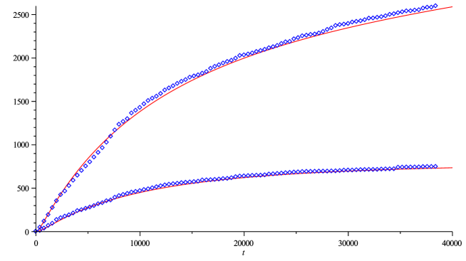
Figure 1: Joint complexity of actual simulated texts (3rd Markov order) of English, vs French (top), Polish (bottom) languages, versus average theoretical (plain).

Here, we derive a second order asymptotics for $J$-complexity for Markov sources of the following form

$$\gamma\frac{n^{\kappa}}{\sqrt{\alpha\log n+\beta}}$$

for some $\beta>0$. This new estimate converges faster, although for small text lengths of order $n\approx 10^{2}$ one needs to compute additional terms. In fact, for some Markov sources our analysis indicates that $J$-complexity oscillates with $n$. This is manifested by appearing a periodic function in the leading term of our asymptotics. Surprisingly, this additional term even further improves the convergence for small values of $n$.

Let us now summarize in full our main results Theorems 1–9. In our first main result Theorem 1 we observe that the joint string complexity $J_{n,m}$ can be asymptotically analyzed by considering a simpler quantity called the joint prefix complexity denoted as $C_{n,m}$. It counts the number of common prefixes of two sets of size $n$ and $m$, respectively, of independently generated strings by two Markov sources. In the reminding part of the paper we only deal with the joint prefix complexity $C_{n,m}$. First in Theorem 2 we considered two statistically identical sources and prove that the joint string complexity grows linearly with $n$: For certain sources called noncommensurable there is a constant in front of $n$ (that we determine) while for commensurable sources the factor in front of $n$ is a fluctuating periodic function of small amplitude. We shall see these two cases permeate all our results. Then we deal in Theorem 3 with a special sources in which the underlying Markov matrices are nilpotent. After that we study general sources, however, we split our presentation and proofs into two parts. First, in Theorems 4–5 we assume that one of the source is uniform. Under this assumption we develop techniques to prove our results. Finally, in Theorem 7 – 9 we discuss general case.

Let us now compare our theoretical results with experimental results on real texts generated in different languages. In Figure 1 we compare the joint complexity of a simulated English text with the same length texts simulated in French and in Polish. In the simulation we use a Markov model of order 3. It is easy to see that even for texts of lengths smaller than a thousand one can discriminate between these languages. In fact, computations show that for English versus French we have $\kappa=0.18$; and versus Polish: $\kappa=0.1$, Furthermore, for a Markov model of order 3 we find that English text has entropy (per symbol): $0.944$; French: $0.934$; Polish: $0.665$. The theoretical curves shown in Figure 1 are obtained through Theorem 8, however, for small values of the text length it is computed via the iterative resolution of functional equations (49) and (51). Figure 2 shows the continuation of our theoretical estimates up to $n=10^{10}$ and compared with the theoretical estimate $O(n^{\kappa})$ as presented in Theorems 7 – 8.

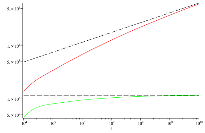
Figure 2: Average theoretical Joint complexity of 3rd Markov order text of English, vs French (top), and vs Polish (bottom) languages, versus order estimate $O(n^{\kappa})$.

It didn’t escape our attention that the joint string complexity can be used to discriminate Markov sources [22] since, as already observed, the growth of the joint string complexity is $O(n^{\kappa})$ with $\kappa=1$ when sources are statistically indistinguishable and $\kappa<1$ otherwise. For example, we can use the joint string complexity to verify authorship of an unknown manuscript by comparing it to a manuscript of known authorship and checking whether $\kappa=1$ or not. More precisely, we propose to introduce the following discriminant function

$$d(X,Y)=1-\frac{1}{\log n}\log J(X,Y)$$

for two sequences $X$ and $Y$ of length $n$. This discriminant allows us to determine whether $X$ and $Y$ are generated by the same Markov source or not by verifying whether $d(X,Y)=O(1/\log n)\to 0$ or $d(X,Y)=1-\kappa+O(\log\log n/\log n)>0$, respectively. In fact, we used it with some success to classify twitter messages (see SNOW 2014 challenge of tweets detection).

The paper is organized as follows. In the next section we present our main results Theorems 1–9. We prove Theorem 1 in Section III. Then we present some preliminary results in Section IV. In particular, we derive the functional equation for the joint prefix complexity $C_{n,m}$, establish some depoissonization results, and derive double Mellin transform. We first prove the nilpotent case in Section V. The proofs of Theorems 4 – 5 are presented in Section VI, and the proofs of Theorem 7 – 9 are discussed in Section VII.

II Main Results

In this section we define precisely our problem, introduce some important notation, and present our main results Theorem 1 – Theorem 9. The proofs are presented in the remaining parts of the paper and Appendix.

II-A Models and notations

We begin by introducing some general notation. Let $X$ and $w$ be two strings over the alphabet ${\mathcal{A}}$. We denote by $|X|_{w}$ the number of times $w$ occurs in $X$ (e.g., $|abbba|_{bb}=2$ when $X=abbba$ and $w=bb$). By convention $|X|_{\nu}=|X|+1$, where $\nu$ is the empty string.

Throughout we denote by $X$ a string (text) whose complexity we plan to study. We also assume that its length $|X|$ is equal to $n$. Then we define $I(X)=\{w:~{}|X|_{w}\geq 1\}$, that is, $I(X)$ contains all distinct subwords of $X$. Observe that the string complexity $|I(X)|$ can be represented as

$$|I(X)|=\sum_{w\in{\mathcal{A}}^{*}}1_{|X|_{w}\geq 1},$$

where $1_{A}$ is the indicator function of the event $A$. Notice that $|I(X)|$ is equal to the number of nodes in the associated suffix tree of $X$ [12, 21] (see also [6]).

Now, let $X$ and $Y$ be two strings (not necessarily of the same length). We define the joint string complexity as the cardinality of the set $J(X,Y)=I(X)\cap I(Y)$, that is,

$$|J(X,Y)|=\sum_{w\in{\mathcal{A}}^{*}}1_{|X|_{w}\geq 1}\times 1_{|Y|_{w}\geq 1}~{}.$$

In other words, $J(X,Y)$ represents the number of common and distinct subwords of both $X$ and $Y$. For example, if $X=aabaa$ and $Y=abbba$, then $J(X,Y)=\{\epsilon,a,b,ab,ba\}$.

In this paper throughout we assume that both strings $X$ and $Y$ are generated by two independent Markov sources of order $r$ (we will only deal here with Markov of order 1, but extension to arbitrary order is straightforward). We assume that source $i$, for $i\in\{1,2\}$ has the transition probabilities $P_{i}(a|b)$ from state $b$ to state $a$, where $a,b\in{\mathcal{A}}^{r}$. We denote by ${\bf P}_{1}$ (resp. ${\bf P}_{2}$) the transition matrix of Markov source 1 (resp. source 2). The stationary distributions are respectively denoted by $\mbox{\boldmath$\pi$}_{1}(a)$ and $\mbox{\boldmath$\pi$}_{2}(a)$ for $a\in{\mathcal{A}}^{r}$. Throughout, we consider general Markov sources with transition matrices ${\bf P}_{i}$ that may contain zero coefficients. This assumption leads to interesting embellishment of our results.

Let $X_{n}$ and $Y_{m}$ be two strings of respective lengths $n$ and $m$, generated by Markov source 1 and Markov source 2, respectively. We write

$$J_{n,m}=\mathbf{E}(|J(X_{n},Y_{m})|)-1=\sum_{w\in{\mathcal{A}}^{*}\setminus\nu}P(|X|_{w}\geq 1)P(|Y|_{w}\geq 1)$$ (1)

for the joint complexity, i.e. omitting the empty string. In this paper we study $J_{n,m}$ for $n=\Theta(m)$.

It turns out that analyzing $J_{n,m}$ is very challenging. It is related to the number of common nodes in two suffix trees, one built for $X$ and the other built for $Y$. We know that analysis of a single suffix tree is quite challenging [6, 18]. Its analysis is reduced to study a simpler structure known as tries, a digital tree built from prefixes of a set of independent strings. We shall follow this approach here. Therefore, we introduce another concept. Let ${\mathcal{X}}$ be a set of infinite strings, and we define the prefix set ${\cal I}({\mathcal{X}})$ of ${\mathcal{X}}$ as the set of prefixes of ${\mathcal{X}}$. Let ${\mathcal{X}}$ and ${\mathcal{Y}}$ be now two sets of strings and we define the joint prefix complexity as the number of common prefixes, i.e. $|{\cal I}({\mathcal{X}})\cap{\cal I}({\mathcal{Y}})|$. When ${\mathcal{X}}_{n}$ is a set of $n$ independent strings generated by source 1 and ${\mathcal{Y}}_{m}$ is a set of $m$ independent strings generated by source 2, then we define $C_{n,m}$ as

$$C_{n,m}=\mathbf{E}|{\cal I}({\mathcal{X}}_{n})\cap{\cal I}({\mathcal{Y}}_{m})|)-1$$

which represents the number of common prefixes between ${\mathcal{X}}_{n}$ and ${\mathcal{Y}}_{m}$.

Observe that we can re-write $C_{n,m}$ in a different way. Define $\Omega^{i}(w)$ for $i=1,2$ as the number of strings in ${\mathcal{X}}$ and ${\mathcal{Y}}$, respectively, whose prefixes are equal to $w$ provided that strings in ${\mathcal{X}}$ are generated by source $1$ and strings in ${\mathcal{Y}}$ by source $2$. Then, it is easy to notice that

$$C_{n,m}=\sum_{w\in{\mathcal{A}}^{*}\setminus\nu}P(\Omega^{1}_{n}(w)\geq 1)P(\Omega^{2}_{m}(w)\geq 1)$$ (2)

which should be compared to (1).

The idea is that $C_{n,m}$ is a good approximation of $J_{n,m}$ as we present in our first main result Theorem 1. We shall see in Sections IV – VII that $C_{n,m}$ are easier to analyze, however, far from simple. In fact, $C_{n,m}$ has a nice interpretation. It corresponds to the number of common nodes in two tries built from ${\mathcal{X}}$ and ${\mathcal{Y}}$. We know [10, 9, 21] that tries are easier to analyze than suffix trees.

II-B Summary of Main Results

We now present our main theoretical results. In the first foundation result below we show that asymptotically we can analyze $J_{n,m}$ through the quantity $C_{n,m}$ defined above in (2). The proof of the next result can be found in Section III.

Theorem 1.

Let $n$ and $m$ be of the same order. Then there exists $1/2\leq\epsilon<1$ such that

$$J_{n,m}=C_{n,m}+O(n^{\epsilon}+m^{\epsilon})$$ (3)

as $n\to\infty$.

In the rest of the paper we shall analyze $C_{n,n}$. We should point out that the error term could be as large as the leading term, but for sources that are relatively close the error term will be negligible.

Now we presents a series of results each treating different cases of Markov sources. However, our results depend on whether the underlying Markov sources are commensurable or not so we define them next.

Definition 1 (Rationally Related Matrix).

We say that a matrix ${\bf M}=[m_{ab}]_{(a,b)\in{\mathcal{A}}^{2}}$ is rationally related if $\forall(a,b,c)\in{\mathcal{A}}^{3}$ we have $m_{ab}+m_{ca}-m_{cb}\in\mathbb{Z},$ where $\mathbb{Z}$ is the set of integers.

Definition 2 (Logarithmically rationally related matrix).

We say that a matrix ${\bf M}=[m_{ab}]$ is logarithmically rationally related if there exists a non zero real number $x$ such that the matrix $x\log^{*}({\bf M})$ is rationally related, where the matrix $\log^{*}({\bf M})$ is composed of $\log(m_{ab})$ when $m_{ab}>0$ and zero otherwise. The smallest non negative value $\omega$ of the real $x$ defined above is called the root of ${\bf M}$.

The following matrix is an example of logarithmically rationally related matrix:

$${\bf P}=\left[\begin{array}[]{cccc}\frac{1}{4}&\frac{1}{8}&\frac{1}{2}&\frac{1}{4}\\ \frac{1}{4}&\frac{1}{8}&\frac{1}{8}&\frac{1}{2}\\ \frac{1}{4}&\frac{1}{4}&\frac{1}{4}&\frac{1}{8}\\ \frac{1}{4}&\frac{1}{2}&\frac{1}{8}&\frac{1}{8}\end{array}\right].$$

Its root is $1/log2$.

Definition 3 (Logarithmically commensurable pair).

We say that a pair of two matrices ${\bf M}=[m_{ab}]_{(a,b)\in{\mathcal{A}}^{2}}$ and ${\bf M}^{\prime}=[m^{\prime}_{ab}]$ is logarithmically commensurable if there exist a pair of real numbers $(x,y)$ such that $x\log^{*}({\bf M})+y\log^{*}({\bf M}^{\prime})$ is not null and is logarithmically rationally related.

Notice that when ${\bf M}$ and ${\bf M}^{\prime}$ are both rationally related, then the pair is logarithmically commensurable. Nevertheless it is possible to have logarithmically commensurable pairs with the individual matrices not logarithmically rationally related. For example when $\log^{*}{\bf M}^{\prime}=2\pi{\bf Q}+\log^{*}{\bf M}$ with ${\bf Q}$ an integer matrix.

We are now in the position to discuss our first main result for Markov sources that are statistically indistinguishable. Throughout we present results for $m=n$.

Theorem 2.

Consider the average joint complexity of two texts of length $n$ generated by the same general stationary Markov source, that is, ${\bf P}:={\bf P}_{1}={\bf P}_{2}$.

(i) [Noncommensurable Case.] Assume that ${\bf P}$ is not logarithmically rationally related. Then

$$J_{n,n}=\frac{2n\log 2}{h}+o(n)$$ (4)

where $h$ is the entropy rate of the source defined as $h=\sum_{a,b\in{\mathcal{A}}}\pi(a)P(a|b)$.

(ii) [Commensurable Case.] Assume that ${\bf P}$ is logarithmically rationally related. Then there is $\epsilon<1$ such that:

$$J_{n,n}=\frac{2n\log 2}{h}(1+Q_{0}(\log n))+O(n^{\epsilon})$$ (5)

where $Q_{0}(.)$ is a periodic function of small amplitude. (In Section IV-C compute explicitly $Q$.)

Now we consider sources that are not the same and have respective transition matrices ${\bf P}_{1}$ and ${\bf P}_{2}$. The transition matrices are on ${\mathcal{A}}^{r}\times{\mathcal{A}}^{r}$. If $(a,b)\in{\mathcal{A}}^{r}\times{\mathcal{A}}^{r}$, we denote by $P_{i}(a|b)$ the $(a,b)$-th coefficient of matrix ${\bf P}_{i}$. For a tuple of complex numbers $(s_{1},s_{2})$ we write ${\bf P}(s_{1},s_{2})$ for the following matrix

$${\bf P}(s_{1},s_{2})=[{\bf P}_{1}(a|b))^{-s_{1}}({\bf P}_{2}(a|b))^{-s_{2}}]_{a,b\in A}.$$

In fact, we can write it as the Schur product, denoted as $\star$, of two matrices ${\bf P}_{1}(s_{1})={\bf P}_{1}(a|b))^{-s_{1}}$ and ${\bf P}_{2}(s_{2})=({\bf P}_{2}(a|b))^{-s_{2}}$, that is, ${\bf P}(s_{1},s_{2})={\bf P}_{1}(s_{1})\star{\bf P}_{2}(s_{2})$.

To present succinctly our general results we need some more notation. Let $\langle{\bf x}|{\bf y}\rangle$ be the scalar product of vector ${\bf x}$ and vector ${\bf y}$. By $\lambda(s_{1},s_{2})$ we denote the main eigenvalue of matrix ${\bf P}(s_{1},s_{2})$, and ${\bf u}(s_{1},s_{2})$ its corresponding right eigenvector (i.e, $\lambda(s_{1},s_{2}){\bf u}(s_{1},s_{2})={\bf P}(s_{1},s_{2}){\bf u}(s_{1},s_{2})$), and $\mbox{\boldmath$\zeta$}(s_{1},s_{2})$ its left eigenvector (i.e., $\lambda(s_{1},s_{2}){\bf u}(s_{1},s_{2})={\bf u}(s_{1},s_{2}){\bf P}(s_{1},s_{2})$). We assume that $\langle\mbox{\boldmath$\zeta$}(s_{1},s_{2})|{\bf u}(s_{1},s_{2})\rangle=1$. Furthermore, the vector ${\boldsymbol{\pi}}(s_{1},s_{2})$ is defined as the vector $(\pi_{1}(a)^{-s_{1}}\pi_{2}(a)^{-s_{2}})_{a\in{\mathcal{A}}}$ where $(\pi_{i}(a))_{a\in{\mathcal{A}}}$ is the left eigenvector of matrix ${\bf P}_{i}$ for $i\in\{1,2\}$. In other words $(\pi_{i}(a))_{a\in{\mathcal{A}}}$ is the stationary distribution of the Markov source $i$.

We start our presentation with the simplest case, namely the case when the matrix ${\bf P}(0,0)$ is nilpotent [13], that is, for some $K$ the matrix ${\bf P}^{K}(0,0)$ is the null matrix. Notice that for nilpotent matrices $\forall(s_{1},s_{2})$:  ${\bf P}^{K}(s_{1},s_{2})=0$.

Theorem 3.

If ${\bf P}(s_{1},s_{2})$ is nilpotent, then there exists $\gamma_{0}$ such that

$$\lim_{n\to\infty}J_{n,n}=\gamma_{0}:=\langle{\bf 1}_{C}({\bf I}-{\bf P}(0,0))^{-1}|{\bf 1}\rangle$$ (6)

where ${\bf 1}$ is the unit vector, ${\bf 1}_{C}$ the vector on ${\mathcal{A}}$ with ${\bf 1}_{C}(a)=1$ when $a$ is common to both sources, and ${\bf 1}_{C}(a)=0$ otherwise.

This result is not surprising and rather trivial since the common factors can only occur in a finite window at the beginning of the strings. It turns out that $\gamma_{0}=1168$ for 3rd order Markov model of English versus Polish languages used in our experiments.

Throughout, now we assume that ${\bf P}(s_{1},s_{2})$ is not nilpotent. We need to pay much closer attention to the structure of the set of roots of the characteristic equation

$$\lambda(s_{1},s_{2})=1$$

that will play a major role in the analysis. We discuss in depth properties of these roots in Section IV-E. Here we introduce only a few important definitions.

Definition 4.

The kernel $\overline{{\cal K}}$ is the set of complex tuples $(s_{1},s_{2})$ such that ${\bf P}(s_{1},s_{2})$ has its largest eigenvalue equal to 1. The real kernel ${\cal K}=\overline{{\cal K}}\cap\mathbb{R}^{2}$, i.e. the set of real tuples $(s_{1},s_{2})$ such that the main eigenvalue $\lambda(s_{1},s_{2})=1$.

The following lemma is easy to prove.

Lemma 1.

The real kernel forms a concave curve in $\mathbb{R}^{2}$.

Furthermore, we introduce two important notations:

$$\kappa = \min_{(s_{1},s_{2})\in{\cal K}}\{-s_{1}-s_{2}\}$$ (7)

$$(c_{1},c_{2}) = \arg\min_{(s_{1},s_{2})\in{\cal K}}\{-s_{1}-s_{2}\}.$$ (8)

This leads to a new concept $\partial{\cal K}$, the border of the kernel $\overline{{\cal K}}$, defined as follows.

Definition 5.

We denote $\partial{\cal K}$ the subset of $\overline{{\cal K}}$ made of the pairs $(s_{1},s_{2})$ such $\Re(s_{1},s_{2})=(c_{1},c_{2})$.

Easy algebra shows that $\kappa\leq 1$. Furthermore, in the Appendix we prove the following property.

Lemma 2.

Let $c_{1}$ and $c_{2}$ minimize $-s_{1}-s_{2}$ where real tuple $(s_{1},s_{2})\in{\cal K}$. Assume $\forall(a,b)\in{\mathcal{A}}^{2}$: $P_{1}(a|b)>0$ then $c_{1}\leq 0$ and $c_{2}\geq-1$.

The case when both matrices ${\bf P}_{1}$ and ${\bf P}_{2}$ have some zero coefficients is the most intricate part. Therefore, to present our strongest results, we start with a special case when one of the source is uniform. Later we generalize it.

We first consider a special case when source 1 is uniform memoryless, i.e. ${\bf P}_{1}=\frac{1}{|{\mathcal{A}}|}{\bf 1}\otimes{\bf 1}$ and the other matrix ${\bf P}_{2}$ is not nilpotent and general (that is, it may have some zero coefficients). In this case we always have $c_{1}<0$ and $c_{2}<0$. This case we have the following theorem.

Theorem 4.

Let ${\bf P}_{1}=\frac{1}{|{\mathcal{A}}|}{\bf 1}\otimes{\bf 1}$ and ${\bf P}_{2}\neq{\bf P}_{1}$ is a general transition matrix. Thus both $c_{1}$ and $c_{2}$ are between $-1$ and $0$.

(i) [Mono periodic case.] If ${\bf P}_{2}$ is not logarithmically rationally related, then there exists a periodic function $Q_{1}(x)$ of small amplitude such that

$$C_{n,n}=\frac{\gamma_{2}n^{\kappa}}{\sqrt{\alpha_{2}\log n+\beta_{2}}}(1+Q_{1}(\log n)+o(1)).$$ (9)

(ii) [Double periodic case.] If ${\bf P}_{2}$ is logarithmically rationally related, then there exists a double periodic function $Q_{2}(.)$ of small amplitude such that

$$C_{n,n}=\frac{\gamma_{2}n^{\kappa}}{\sqrt{\alpha_{2}\log n+\beta_{2}}}(1+Q_{2}(\log n)+o(1)).$$ (10)

The constants $\gamma_{2}$, $\alpha_{2}$ and $\beta_{2}$ in the Theorem 4 are explicitly computable as presented next. To simplify our notation for all $(a,b)\in{\mathcal{A}}^{2}$ we shall write $P_{2}(a|b)=P(a|b)$ and ${\bf P}_{2}={\bf P}$. Therefore

$${\bf P}(s_{1},s_{2})=|{\mathcal{A}}|^{s_{1}}{\bf P}(s)$$ (11)

with ${\bf P}(s)={\bf P}(0,s)$. We also write $\pi(a)=\pi_{2}(a)$ and ${\boldsymbol{\pi}}(s)=[\pi(a)^{-s}]_{a\in{\mathcal{A}}}$, thus

$${\boldsymbol{\pi}}(s_{1},s_{2})=|{\mathcal{A}}|^{s_{1}}{\boldsymbol{\pi}}(s_{2})~{}.$$ (12)

Let $\lambda(s_{1},s_{2})$ be again the main (largest) eigenvalue of ${\bf P}(s_{1},s_{2})$. We have

$$\lambda(s_{1},s_{2}))=|{\mathcal{A}}|^{s_{1}}\lambda(s_{2})$$ (13)

where $\lambda(s)$ is the main eigenvalue of matrix ${\bf P}(s)$. We also define ${\bf u}(s)$ as the right eigenvector of ${\bf P}(s)$ and $\mbox{\boldmath$\zeta$}(s)$ as the left eigenvector provided $\langle\mbox{\boldmath$\zeta$}(s)|{\bf u}(s)\rangle=1$. It is easy to see that

$$\lambda(s)=\langle\mbox{\boldmath$\zeta$}(s)|{\bf P}(s){\bf u}(s)\rangle.$$

Now we can express $c_{1}$ and $c_{2}$ defined in (8) in another way, Notice that if $\lambda(s_{1},s_{2})=1$, then in this case

$$s_{1}=-\log_{|{\mathcal{A}}|}\lambda(s_{2}).$$

Define $L(s)=\log_{|{\mathcal{A}}|}\lambda(s)$. Then $c_{2}$ is the value that minimizes $L(s)-s$, that is,

$$\frac{\lambda^{\prime}(c_{2})}{\lambda(c_{2})}=\log|{\mathcal{A}}|.$$ (14)

Also $c_{1}=-L(c_{2})$ and $\kappa=-c_{1}-c_{2}=\min_{s}\{L(s)-s\}$. We have $\kappa\leq 1$ since $L(0)=1$.

We now can presents explicit expression for the constants in Theorem 4.

Theorem 5.

We consider the case ${\bf P}_{1}=\frac{1}{|{\mathcal{A}}|}{\bf 1}\otimes{\bf 1}$ and ${\bf P}_{2}\neq{\bf P}_{1}$ has all non negative coefficients. Let $f(s)=\langle{\boldsymbol{\pi}}(s)|{\bf u}(s)\rangle$ and $g(s)=\langle\mbox{\boldmath$\zeta$}(s)|{\bf 1}\rangle$. Furthermore, with $\Psi(s)$ being the Euler psi function, define $\alpha_{2}=L^{\prime\prime}(c_{2})$ where $L(s)=\log_{|{\mathcal{A}}|}\lambda(s)$, and

$$\beta_{2}(s_{1},s_{2})=-\alpha_{2}\left(\Psi(s_{1})+\frac{1}{1+s_{1}}+\log|{\mathcal{A}}|\right)$$

$$+\Psi^{\prime}(s_{1})-\frac{1}{(s_{1}+1)^{2}}+\Psi^{\prime}(s_{2})-\frac{1}{(s_{2}+1)^{2}}$$

$$+\frac{f^{\prime\prime}(s_{2})}{f(s_{2})}-\left(\frac{f^{\prime}(s_{2})}{f(s_{2})}\right)^{2}+\frac{g^{\prime\prime}(s_{2})}{g(s_{2})}-\left(\frac{g^{\prime}(s_{2})}{g(s_{2})}\right)^{2}$$

as well as

$$\gamma(s_{1},s_{2})=\frac{f(s_{1})g(s_{2})(s_{1}+1)\Gamma(s_{1})(s_{2}+1)\Gamma(s_{2})}{\lambda(s_{2})\log|{\mathcal{A}}|\sqrt{2\pi}}.$$

We have $c_{1}=-\log_{|{\mathcal{A}}|}\lambda(c_{2})$, and then

$$C_{n,n} = n^{\kappa}\frac{\gamma(c_{1},c_{2})}{\sqrt{\alpha_{2}\log n+\beta_{2}(c_{1},c_{2})}}$$ (15)

$$+n^{\kappa}Q(\log n)+o(\frac{n^{\kappa}}{\sqrt{\log n}}).$$

The function $Q(x)$ can be expressed as

$$Q(x)=\sum_{(s_{1},s_{2})\in\partial{\cal K}^{*}}e^{ix\Im(s_{1}+s_{2})}\frac{\gamma(s_{1},s_{2})}{\sqrt{\alpha_{2}x+\beta_{2}(s_{1},s_{2})}}.$$

If the matrix ${\bf P}_{2}$ is logarithmically rationally related, then $\partial{\cal K}$ is a lattice. Let $\omega$ the root of ${\bf P}_{2}$ then

$$\partial{\cal K}=\left\{\left(c_{1}+\frac{2ik\pi}{\log|{\mathcal{A}}|},c_{2}+2i\pi\ell\omega\right),k,\ell)\in\mathbb{Z}^{2}\right\},$$

and $\sqrt{x}Q(x)$ is asymptotically double periodic. Otherwise (i.e., irrational case),

$$\partial{\cal K}=\left\{\left(c_{1}+\frac{2ik\pi}{\log 2},c_{2}\right),~{}k\in\mathbb{Z}\right\}$$

and $\sqrt{x}Q(x)$ is asymptotically single periodic. The amplitude of $Q$ is of order $10^{-6}$.

Now we consider the case when the matrices ${\bf P}_{1}$ and ${\bf P}_{2}$ are general and ${\bf P}_{1}\neq{\bf P}_{2}$. If they contain some zero coefficients, then we may have ${\bf P}(-1,0)\neq{\bf P}_{1}$ and/or ${\bf P}(0,-1)\neq{\bf P}_{2}$. In this (very unlikely) case we may have ${\bf P}(-1,0)={\bf P}(0,-1)$ or more generally they are conjugate. For example for matrices:

$${\bf P}_{1}=\left[\begin{array}[]{cccc}0&0&\frac{5}{8}&\frac{1}{2}\\ 0&\frac{1}{8}&\frac{1}{8}&\frac{1}{4}\\ \frac{1}{2}&\frac{1}{4}&\frac{1}{4}&\frac{1}{8}\\ \frac{1}{2}&\frac{5}{8}&0&\frac{1}{8}\end{array}\right]{\bf P}_{2}=\left[\begin{array}[]{cccc}\frac{1}{2}&\frac{5}{8}&0&\frac{1}{2}\\ \frac{1}{2}&\frac{1}{8}&\frac{1}{8}&\frac{1}{4}\\ 0&\frac{1}{4}&\frac{1}{4}&\frac{1}{8}\\ 0&0&\frac{5}{8}&\frac{1}{8}\end{array}\right]$$

we have

$${\bf P}(-1,0)={\bf P}(0,-1)=\left[\begin{array}[]{cccc}0&0&0&\frac{1}{2}\\ 0&\frac{1}{8}&\frac{1}{8}&\frac{1}{4}\\ 0&\frac{1}{4}&\frac{1}{4}&\frac{1}{8}\\ 0&0&0&\frac{1}{8}\end{array}\right]$$

If ${\bf P}(-1,0)={\bf P}(0,-1)$, then there is no unique solution $(c_{1},c_{2})$ of the characteristic equation, and therefore there is no saddle point. As a consequence, we have the following theorem:

Theorem 6.

When ${\bf P}(-1,0)$ and ${\bf P}(0,-1)$ are conjugate matrices we have

$$C_{n,n}=\gamma_{0}(-\kappa)n^{\kappa}(1+o(1))$$ (16)

where $\kappa<1$ is such that $(-\kappa,0)\in{\cal K}$ and $\gamma_{0}(-\kappa)$ are explicitly computable. When both matrices are logarithmically rationally related, then

$$C_{n,n}=\gamma(-\kappa)n^{\kappa}\left(1+Q_{0}(\log n)+O(n^{-\epsilon}\right)$$ (17)

where $Q_{0}(.)$ is small periodic function and $\epsilon>0$.

In general, however, ${\bf P}(-1,0)$ and ${\bf P}(0,-1)$ are not conjugate, and therefore, there is a unique $(c_{1},c_{2})$ of the characteristic equation $\lambda(c_{1},c_{2})=1$. As in the special case discussed above, $c_{1}>-1$ and $c_{2}>-1$, however, our results are quantitatively different when $c_{1}>0$ or $c_{2}>0$. We consider it first in Theorem 7 below. Since both cases cannot occur simultaneously, we dwell only on the case $c_{2}>0$; the case $c_{1}>0$ can be handled in a similar manner.

Theorem 7.

Assume ${\bf P}(0,0)$ is not nilpotent and $c_{2}>0$.

(i) [Noncommensurable Case.] We assume that ${\bf P}(-1,0)$ is not logarithmically related. Let $-1<c_{0}<0$ such that $(c_{0},0)\in{\cal K}$. There exist $\gamma_{1}$ such that

$$C_{n,n}=\gamma_{1}n^{-c_{0}}(1+o(1))$$ (18)

(ii) [Commensurable Case.] Let now ${\bf P}(-1,0)$ be logarithmically rationally related. There exists a periodic function $Q_{1}(.)$ of small amplitude such that

$$C_{n,n}=\gamma_{1}n^{-c_{0}}(1+Q_{1}(\log n)+O(n^{-\epsilon}).$$ (19)

Finally, we handle the most intricate case when both $c_{1}$ and $c_{2}$ are between $-1$ and $0$. Recall that when both matrix ${\bf P}_{1}$ and ${\bf P}_{2}$ have all positive coefficients, then ${\bf P}(-1,0)={\bf P}_{1}$ and ${\bf P}(0,-1)={\bf P}_{2}$.

Theorem 8.

Assume that both $c_{1}$ and $c_{2}$ are between $-1$ and $0$ and ${\bf P}(0,0)$ is not nilpotent.

(i) [Non periodic Case.] If ${\bf P}(-1,0)$ and ${\bf P}(0,-1)$ are not logarithmically commensurable matrices, then there exist $\alpha_{2}$, $\beta_{2}$ and $\gamma_{2}$ such that

$$C_{n,n}=\frac{\gamma_{2}n^{\kappa}}{\sqrt{\alpha_{2}\log n+\beta_{2}}}(1+o(1)).$$ (20)

(ii) [Mono periodic case.] If only one of the matrices ${\bf P}(-1,0)$ and ${\bf P}(0,-1)$ is logarithmically rationally related, then there exists a periodic function $Q_{2}(x)$ of small amplitude such that

$$C_{n,n}=\frac{\gamma_{2}n^{\kappa}}{\sqrt{\alpha_{2}\log n+\beta_{2}}}(1+Q_{1}(\log n)+o(1)).$$ (21)

(iii) [Double periodic case.] If both matrices ${\bf P}_{1}$ and ${\bf P}_{2}$ are logarithmically rationally related, then function $Q_{2}(.)$ is double periodic with small amplitude such that

$$C_{n,n}=\frac{\gamma_{2}n^{\kappa}}{\sqrt{\alpha_{2}\log n+\beta_{2}}}(1+Q_{2}(\log n)+o(1)).$$ (22)

In the three cases the constants $\gamma_{2}$, $\alpha_{2}$ and $\beta_{2}$ are explicitly computable.

Remark In the rational case, the root can be such that $\omega\log|{\mathcal{A}}|$ is rational. In this case $\sqrt{x}Q(x)$ tends to a simple periodic function instead of a double periodic function.

At last, we provide explicit expression for some of constants in previously stated results, in particular in the most interesting Theorem 8. We denote $H(s_{1},s_{2})=1-\lambda(s_{1},s_{2})$. Let $H_{1}(s_{1},s_{2})=\frac{\partial}{\partial s_{1}}\lambda(s_{1},s_{2})$, $f(s_{1},s_{2})=\langle{\boldsymbol{\pi}}(s_{1},s_{2})|{\bf u}(s_{1},s_{2})\rangle$ and $g(s_{1},s_{2})=\langle\mbox{\boldmath$\zeta$}(s_{1},s_{2})|{\bf 1}\rangle$.

Theorem 9.

Let $c_{1}$ and $c_{2}$ be between $-1$ and $0$. In the general case we have

$$C_{n,n}=n^{\kappa}\sum_{(s_{1},s_{2})\in\partial{\cal K}}\frac{\gamma(s_{1},s_{2})n^{-i\Im(s_{1}+s_{2})}}{\sqrt{\alpha_{2}\log n+\beta(s_{1},s_{2})}}\left(1+O(\frac{1}{\log n})\right).$$ (23)

With $H_{1}$, $\alpha_{2}$, $\beta_{2}(s_{1},s_{2})$ and $\gamma(s_{1},s_{2})$ such

$$H_{1} = \frac{\partial}{\partial s_{1}}H(c_{1},c_{2})$$

$$\alpha_{2} = \frac{\Delta H-2\frac{\partial^{2}}{\partial s_{1}\partial s_{2}}H}{H_{1}}|_{(s_{1},s_{2})=(c_{1},c_{2})}$$

$$\beta_{2}(s_{1},s_{2}) = -\frac{\alpha_{2}}{2}\left(\Psi(s_{1})+\Psi(s_{2})+\frac{\frac{\partial}{\partial s_{1}}f+\frac{\partial}{\partial s_{2}}f}{f}+\frac{\frac{\partial}{\partial s_{1}}g+\frac{\partial}{\partial s_{2}}g}{g}\right)$$

$$+\Psi^{\prime}(s_{1})+\Psi^{\prime}(s_{2})+\frac{\Delta f-2\frac{\partial^{2}}{\partial s_{1}\partial s_{2}}f}{f}+\frac{\Delta g-2\frac{\partial^{2}}{\partial s_{1}\partial s_{2}}g}{g}$$

$$-\left(\frac{\frac{\partial}{\partial s_{1}}f-\frac{\partial}{\partial s_{2}}f}{f}\right)^{2}-\left(\frac{\frac{\partial}{\partial s_{1}}g-\frac{\partial}{\partial s_{2}}g}{g}\right)^{2}$$

$$+\frac{\alpha_{2}^{2}}{2}-\frac{\frac{\partial^{3}}{\partial s_{1}^{3}}H-\frac{\partial^{3}}{\partial s_{1}^{2}\partial s_{2}}H-\frac{\partial^{3}}{\partial s_{1}\partial s_{2}^{2}}H+\frac{\partial^{3}}{\partial s_{2}^{3}}H}{2H_{1}}+\left(\frac{\frac{\partial^{2}}{\partial s_{1}^{2}}H-\frac{\partial^{2}}{\partial s_{2}^{2}}H}{2H_{1}}\right)^{2}$$

and

$$\gamma(s_{1},s_{2})=\frac{f(s_{1})g(s_{2})(s_{1}+1)\Gamma(s_{1})(s_{2}+1)\Gamma(s_{2})}{\lambda(s_{2})\log|{\mathcal{A}}|\sqrt{2\pi}}.$$

The expression for $\alpha_{2}$ seems to be asymmetric in $(s_{1},s_{2})$. In fact, it is not since the maximum of $s_{1}+s_{2}$ for $(s_{1},s_{2})\in{\cal K}$ attained on $(c_{1},c_{2})$ necessarily implies that $\frac{\partial}{\partial s_{1}}H(c_{1},c_{2})=\frac{\partial}{\partial s_{2}}H(c_{1},c_{2})$. Formally the constant $\alpha_{2}$ is equal to $\Delta\lambda_{1}(c_{1},c_{2})\langle{\bf 1}|\nabla\lambda_{1}(c_{1},c_{2})\rangle$ where $\nabla$ is the gradient operator, $\Delta$ the Laplacian operator $\frac{\partial^{2}}{\partial s_{1}^{2}}+\frac{\partial^{2}}{\partial s_{2}^{2}}$.

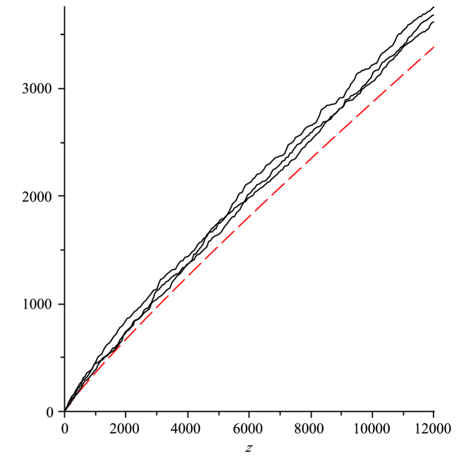
Figure 3: Joint complexity: three simulated trajectories (black) versus asymptotic average (dashed red) for the case $c_{2}>0$.

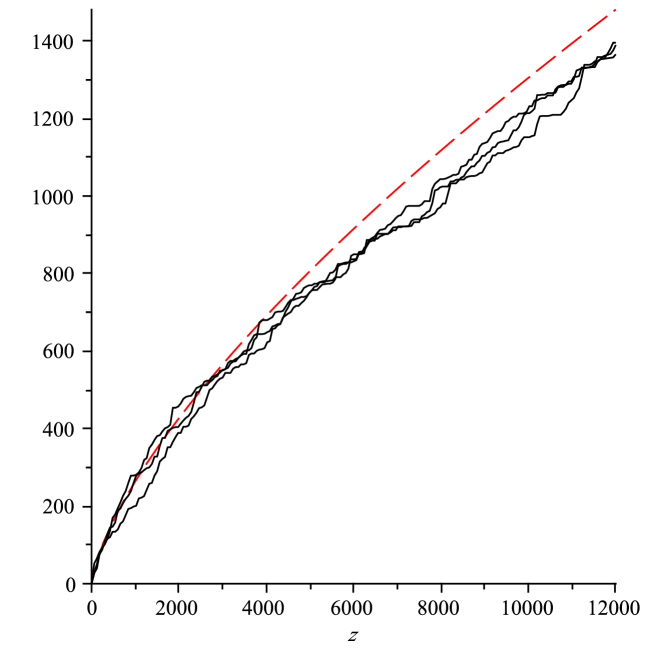
Figure 4: Joint semi-complexity: three simulated trajectories (black) versus asymptotic average (dashed red)for the case $c_{2}<0$.

Finally, we illustrate our results on two examples.

Example. In Figures 3 and 4 we plot the joint complexity for several pairs of strings $X$ and $Y$. String $X$ is generated by a Markov source with the transition matrix ${\bf P}$, and string $Y$ is generated by a uniform memoryless source. We consider two Markov sources for $X$ with the following transition matrix:

$${\bf P}=\left[\begin{array}[]{cc}0&0.5\\ 1&0.5\end{array}\right]\hskip 56.9055pt{\bf P}=\left[\begin{array}[]{cc}0.2&0.8\\ 0.8&0.2\end{array}\right].$$ (24)

For the first ${\bf P}$ in Figure 3 we have $c_{2}>0$ (see Theorem 7) while for the second ${\bf P}$ in Figure 4 we have $c_{2}<0$ (cf. Theorem 4(i)).

III Proof of Theorem 1

We recall that $X$ and $Y$ are two independent strings of length $n$ and $m$, generated by two Markov sources characterized by transition matrices ${\bf P}_{1}$ and ${\bf P}_{2}$, respectively. In the previous section we write $|X|_{w}$ and $|Y|_{w}$ for the number of $w\in{\mathcal{A}}$ occurrences in $X$ and $Y$. But it will be convenient to use another notation for these quantities, namely

$$O^{1}_{n}(w):=|X|_{w},\ \ \ \ O^{2}_{m}(w):=|Y|_{w}.$$

We shall use this notation interchangeably. Finally, we write ${\mathcal{A}}^{+}={\mathcal{A}}^{*}-\{\nu\}$, that is, for the set of all nonempty words. As observed in (1) we have

$$J_{n,m}=\sum_{w\in{\mathcal{A}}^{+}}P(O_{n}^{1}(w)\geq 1)P(O_{m}^{2}(w)\geq 1).$$ (25)

In [20, 9] the generating function of $P(O_{n}(w)\geq 1)$ for a Markov source is derived. It involves the autocorrelation polynomial of $w$, as discussed below. However, to make our analysis tractable we notice that $O_{n}^{i}(w)\geq 1$, $i=1,2$, is equivalent to $w$ being a prefix of at least one of the $n$ suffixes of $X$. But this is not sufficient to push forward our analysis. We need a second much deeper observation that replaces dependent suffixes with independent strings to shift analysis from suffix trees to tries, as already observed in [6] and briefly discussed in Section II. In order to accomplish it, we consider two sets of strings of size $n$ and $m$, respectively, generated independently by Markov sources ${\bf P}_{1}$ and ${\bf P}_{2}$. As in Section II we denote by $\Omega_{n}^{i}(w)$ the number of strings for which $w$ is a prefix when there are $n$ strings generated by source $i$, for $i\in\{1,2\}$. The average joint prefix complexity satisfies (2) that we repeat below

$$C_{n,m}=\sum_{w\in{\mathcal{A}}^{+}}P(\Omega^{1}_{n}(w)\geq 1)P(\Omega^{2}_{m}(w)\geq 1).$$ (26)

Before we prove our first main result Theorem 1 we need some preliminary work. First, observe that it is relatively easy to compute the probability $P(\Omega^{i}_{n}(w)\geq 1)$. Indeed,

$$P(\Omega^{i}_{n}(w)\geq 1)=1-(1-P_{i}(w))^{n}.$$

Notice that the quantity $1-(1-P(w))^{n}$ is the probability that $|{\mathcal{X}}_{n}|_{w}>0$ where ${\mathcal{X}}_{n}$ is a set of $n$ independently generated strings. To prove Theorem 1 we must show that when $n\to\infty$

$$P(O_{n}^{i}(w)\geq 1)\sim P(\Omega^{i}_{n}(w)\geq 1)$$

which we do in the next key lemma.

We denote by ${\cal B}_{k}$ the set of words of length $k$ such that a word $w\in{\cal B}_{k}$ does not overlap with itself over more than $k/2$ characters (see [9, 6, 18] for more precise definition). It is proven in [18] that

$$\sum_{w\in{\mathcal{A}}^{k}-{\cal B}_{k}}P(w)=O(\delta_{1}^{k})$$

where $\delta_{1}<1$ is the largest element of the Markovian transition matrix ${\bf P}$. In order to allow some transition probabilities to be equal to $0$ we define

$$p = \exp\left(\lim\sup_{k,w\in{\mathcal{A}}^{k}}\frac{\log P(w)}{k}\right)$$

$$q = \exp\left(\lim\inf_{k,w\in{\mathcal{A}}^{k},P(w)\neq 0}\frac{\log P(w)}{k}\right).$$

These quantities exist and are smaller than 1 since ${\mathcal{A}}$ is a finite alphabet [19, 21]. In fact, they are related to Renyi’s entropy of order $\pm\infty$, respectively [21]. We write $\delta=\sqrt{p}<1.$

Let $X_{n}$ be a string of length $n$ generated by a Markov source. For $w\in{\mathcal{A}}^{*}$, define

$$d_{n}(w)=P(O_{n}(w)>0)-(1-(1-P(w))^{n}).$$ (27)

We prove the following lemma

Lemma 3.

Let $w\in{\mathcal{A}}^{k}$ be of length $k$. There exists $\rho>1$ and a sequence $R_{n}(w)=O(P(w)\rho^{-n})$ such that for all $1>\epsilon>0$ we have:

(i) for $w\in{\cal B}_{k}$: $d_{n}(w)=O((nP(w))^{\epsilon}k\delta^{k})+R_{n}(w)$;

(ii) for $w\in{\mathcal{A}}^{k}-{\cal B}^{k}$: $d_{n}(w)=O((nP(w))^{\epsilon}\delta^{k})+R_{n}(w)$.

Proof.

Let $N_{0}(z)=\sum_{n\geq 0}P(O_{n}(w)=0)z^{n}$. We know from [9] that

$$N_{0}(z)=\frac{S_{w}(z)}{D_{w}(z)}$$

where $S_{w}(z)$ is the autocorrelation polynomial of word $w$ and $D_{w}(z)$ is defined as follows

$$D_{w}(z)=S_{w}(z)(1-z)+z^{k}P(w)\left(1+F_{w_{1},w_{k}}(z)(1-z)\right),$$ (28)

where $k=|w|$ is the length of word $w$ with first symbol $w_{1}$ and the last symbol $w_{k}$. Here $F_{a,b}(z)$ for $(a,b)\in{\mathcal{A}}^{2}$ is a generating function that depends on the Markov sources, as describe below. We also write $F_{w}(z)$ when $w_{1}=a$ and $w_{k}=b$.

Let ${\bf P}$ be the transition matrix of the Markov source. Let ${\boldsymbol{\pi}}$ be its stationary vector and for $a\in{\mathcal{A}}$ let $\pi_{a}$ be its coefficient at symbol $a$. The vector ${\bf 1}$ is the vector with all coefficients equal to 1 and ${\bf I}$ is the identity matrix. Assuming that the symbol $a$ (resp. $b$) is the first (resp. last) character of $w$, we have [20]

$$F_{w}(z):=F_{a,b(z)}=\frac{1}{\pi_{a}}\left[({\bf P}-{\boldsymbol{\pi}}\otimes{\bf 1})\left({\bf I}-z({\bf P}+{\boldsymbol{\pi}}\otimes{\bf 1})\right)^{-1}\right]_{a,b}$$ (29)

where $[A]_{a,b}$ denotes the $(a,b)$th coefficient of matrix $A$. An alternative way to express $F_{w}(z)$ is

$$F_{w}(z)=\frac{1}{\pi_{a}}\langle{\bf e}_{a}({\bf P}-{\boldsymbol{\pi}}\otimes{\bf 1})\left({\bf I}-z({\bf P}+{\boldsymbol{\pi}}\otimes{\bf 1})\right)^{-1}{\bf e}_{b}\rangle$$ (30)

where ${\bf e}_{c}$ for $c\in{\mathcal{A}}$ is the vector with a 1 at the position corresponding to symbol $c$ and all other coefficients are 0.

By the spectral representation of matrix ${\bf P}$ we have [13]

$${\bf P}={\boldsymbol{\pi}}\otimes{\bf 1}+\sum_{i>1}\lambda_{i}{\bf u}_{i}\otimes\mbox{\boldmath$\zeta$}_{i}$$

where $\lambda_{i}$ for $i\geq 1$ is the $i$th eigenvalue (in decreasing order) of matrix ${\bf P}$ (with $\lambda_{1}=1$), and ${\bf u}_{i}$ (resp. $\mbox{\boldmath$\zeta$}_{i}$) are their corresponding right (resp. left) eigenvectors. Thus

$$({\bf P}-{\boldsymbol{\pi}}\otimes{\bf 1})\left({\bf I}-z({\bf P}+{\boldsymbol{\pi}}\otimes{\bf 1})\right)^{-1}=\sum_{i>1}\frac{\lambda_{i}}{1-\lambda_{i}z}{\bf u}_{i}\otimes\mbox{\boldmath$\zeta$}_{i}$$ (31)

and therefore the function $F_{w}(z)$ is defined for all $z$ such that $|z|<\frac{1}{|\lambda_{2}|}$ and is uniformly $O(\frac{1}{1-|\lambda_{2}z|})$.

We now follow the approach from [18] that extends to Markovian sources the analysis presented in [6] for memoryless sources (see also [9]). Let

$$\Delta_{w}(z)=\sum_{n\geq 0}d_{n}(w)z^{n}$$

be the generating function of $d_{n}(w)$ defined in (27). After some algebra we arrive at

$$\Delta_{w}(z) = \frac{P(w)z}{1-z}\left(\frac{1+(1-z)F_{w}(z)}{D_{w}(z)}-\frac{1}{1-z+P(w)z}\right).$$ (32)

We have

$$d_{n}(w)=\frac{1}{2i\pi}\oint\Delta_{w}(z)\frac{dz}{z^{n+1}},$$

integrated on any loop encircling the origin in the definition domain of $d_{w}(z)$. Extending the result from [6], the authors of [18] show that there exists $\rho>1$ such that the function $D_{w}(z)$ defined in (28) has a single root in the disk of radius $\rho$. Let $A_{w}$ be this root. We have via the residue formula

$$d_{n}(w)=\hbox{\rm Res}(\Delta_{w}(z),A_{w})A_{w}^{-n}-(1-P(w))^{n}+d_{n}(w,\rho)$$ (33)

where $\hbox{\rm Res}(f(z),A)$ denotes the residue of function $f(z)$ on complex number $A$. Thus

$$d_{n}(w,\rho)=\frac{1}{2i\pi}\oint_{|z|=\rho}\Delta_{w}(z)\frac{dz}{z^{n+1}}.$$ (34)

We have

$$\hbox{\rm Res}(\Delta_{w}(z),A_{w})=\frac{P(w)\left(1+(1-A_{w})F_{w}(A_{w})\right)}{(1-A_{w})C_{w}}$$ (35)

where $C_{w}=D^{\prime}_{w}(A_{w})$. But since $D_{w}(A_{w})=0$ we can write

$$\hbox{\rm Res}(\Delta_{w}(z),A_{w})=-\frac{A_{w}^{-k}S_{w}(A_{w})}{C_{w}}.$$ (36)

We can take the asymptotic expansion of $A_{w}$ and $C_{w}$ as it is described in [9], in Lemma 8.1.8 and Theorem 8.2.2. Anyhow the expansions were done in the memoryless case. But an extension to Markov sources simply consists in replacing $S_{w}(1)$ into $S_{w}(1)+P(w)F_{w}(1)$, so we find

$$\left\{\begin{array}[]{rcl}A_{w}&=&1+\frac{P(w)}{S_{w}(1)}\\ &&+P^{2}(w)\left(\frac{k-F_{w}(1)}{S^{2}_{w}(1)}-\frac{S_{w}^{\prime}(1)}{S^{3}_{w}(1)}\right)+O(P(w)^{3}),\\ C_{w}&=&-S_{w}(1)+P(w)\left(k-F_{w}(1)-2\frac{S_{w}^{\prime}(1)}{S_{w}(1)}\right)\\ &&+O(P(w)^{2}).\end{array}\right.$$ (37)

These expansions also appear in [18].

¿From now the proof takes the same path as the proof of Theorem 8.2.2 in [9]. We define the function

$$d_{w}(x)=\frac{A_{w}^{-k}S_{w}(A_{w})}{C_{w}}A_{w}^{-x}-(1-P(w))^{x}.$$ (38)

More precisely, we define the function $\bar{d}_{w}(x)=d_{w}(x)-d_{w}(0)e^{-x}$. Its Mellin transform [21] is

$$d^{*}_{w}(s)\Gamma(s)=\int_{0}^{\infty}\bar{d}_{w}(x)x^{s-1}dx$$

defined for all $\Re(s)\in(-1,0)$ with

$$d_{w}^{*}(s) = \frac{A_{w}^{-k}S_{w}(A_{w}}{C_{w}}((\log A_{w})^{-s}-1)$$ (39)

$$+1-\left(-\log(1-P(w)))\right)^{-s}$$

where $\Gamma(s)$ is the Euler gamma function. When $w\in{\cal B}_{k}$ with the expansion of $A_{w}$ and since $S_{w}(1)=1+O(\delta^{k})$ and $S^{\prime}_{w}(1)=O(k\delta^{k})$, we find that similarly as in [9]

$$d^{*}_{w}(s)=O(|s|k\delta^{k})P(w)^{1-s}$$ (40)

and therefore by the reverse Mellin transform, for all $1>\epsilon>0$:

$$\bar{d}_{w}(n) = \frac{1}{2i\pi}\int_{-\epsilon-i\infty}^{-\epsilon+i\infty}d^{*}_{w}(s)\Gamma(s)s^{-n}ds$$ (41)

$$= O(n^{\epsilon}P(w)^{\epsilon}k\delta^{k}).$$

When $w\in{\mathcal{A}}^{k}-{\cal B}_{k}$ it is not true that $S_{w}(1)=1+O(\delta^{k})$, thus it is shown in [18] that there exists $\alpha>0$ such that for all $w\in{\mathcal{A}}^{*}$: $S_{w}(z)>\alpha$ for all $z$ such that $|z|\leq\rho$. Therefore we get $\bar{d}_{w}(n)=O(n^{\epsilon}P(w)^{\epsilon})$.

We set

$$R_{n}(w)=d_{w}(0)e^{-n}+d_{n}(w,\rho).$$ (42)

We first investigate the quantity $d_{w}(0)$. We prove that $d_{w}(0)=O(P(w))$. Noticing that

$$S_{w}(A_{w})=S_{w}(1)+\frac{P(w)}{S_{w}(1)}S_{w}^{\prime}(1)+O(P(w)^{2})$$

we have the expansion

$$-\frac{A_{w}^{-k}S_{w}(A_{w})}{C_{w}}=1-\frac{P(w)}{S_{w}(1)}\left(F_{w}(1)+\frac{S_{w}^{\prime}(1)}{S_{w}(1)}\right)+O(P(w)^{2}).$$ (43)

Thus

$$d_{w}(0)=-\frac{P(w)}{S_{w}(1)}\left(F_{w}(1)+\frac{S_{w}^{\prime}(1)}{S_{w}(1)}\right)+O(P(w))^{2}).$$ (44)

Thus $d_{w}(0)=O(P(w))$.

Now we need to consider $d_{n}(w,\rho)$. Since $\Delta_{n}(z)$ is clearly $O(P(w))$ and the integral $\oint\Delta(z)\frac{dz}{z^{n+1}}$ is over the circle of radius, the result is $O(P(w)\rho^{-n})$. ∎

Now we are ready to prove Theorem 1.

Proof.

Again staring with

$$J_{n,m}=\sum_{w\in{\mathcal{A}}^{*}}P(O^{1}_{n}(w)>0)P(O^{2}_{m}(w)>0)$$ (45)

we note that

$$P(O^{1}_{n}(w)>0)) = 1-(1-P_{1}(w))^{n}+d^{1}_{n}(w),$$

$$P(O^{2}_{m}(w)>0) = 1-(1-P_{2}(w))^{m}+d^{2}_{m}(w).$$

Thus

$$J_{n,m} = C_{n,m}+\sum_{w\in{\mathcal{A}}}d_{n}^{1}(w)P(O^{2}_{m}>0)$$ (46)

$$+ \sum_{w\in{\mathcal{A}}}(1-(1-P_{1}(w))^{n})d_{m}^{2}(w).$$

We will develop the proof for the first sum, since the proof for the second proof being somewhat similar. When $w\in{\cal B}_{k}$, we have for all $\epsilon>0$

$$d^{1}_{n}(w)=O(n^{\epsilon}P_{1}(w)^{\epsilon}k\delta_{1}^{k})+R^{1}_{n}(w)$$ (47)

and the $R_{n}^{1}(w)$ terms are all $O(P_{1}(w)\rho^{-n})$. We look at the sum

$$\sum_{k}\sum_{w\in{\cal B}_{k}}n^{\epsilon}P(w)^{\epsilon}k\delta_{1}^{k}.$$

It is smaller than

$$\sum_{k}\sum_{w\in{\mathcal{A}}^{k}}n^{\epsilon}P_{1}(w)k(q^{\epsilon-1}\delta_{1})^{k}$$

which is equal to $n^{\epsilon}\sum_{k}k(q^{\epsilon-1}\delta_{1})^{k}$. By choosing a value $\epsilon_{1}$ of $\epsilon$ enough close to $1$ so that $q^{\epsilon_{1}-1}\delta_{1}<1$ we have the $n^{\epsilon_{1}}$ order. Notice that with $\delta_{1}=\sqrt{p}$ we must conclude that $1/2<\epsilon_{1}<1$.

When $w\in{\mathcal{A}}^{k}-{\cal B}_{k}$ the $\delta_{1}^{k}$ factor disappears in the right-hand side expression for $d^{1}_{n}(w)$. But in this case

$$\sum_{w\in{\mathcal{A}}^{k}-{\cal B}_{k}}n^{\epsilon}P(w)(q^{\epsilon-1})^{k}=O(n^{\epsilon}\delta_{1}^{k}(q^{\epsilon-1})^{k},$$

and we conclude similarly.

It remains the sum $\sum_{w\in{\mathcal{A}}^{*}}R_{n}^{1}(w)P_{2}(O_{m}(w)>0)$. For this we remark that $P_{2}(O_{m}(w)>0)=O(mP_{2}(w))$. Therefore the sum is of order $\rho^{-n}m\sum_{w\in{\mathcal{A}}^{*}}P_{1}(w)P_{2}(w)$. It turns out that

$$\sum_{w\in{\mathcal{A}}^{k}}P_{1}(w)P_{2}(w)=O(\lambda_{12}^{k})$$

where $\lambda_{12}$ is the main eigenvalue of the Shur product matrix ${\bf P}_{1}\star{\bf P}_{2}$ (also known denoted ${\bf P}(-1,-1)$. Since $\lambda_{12}<1$ the sum converges and is $O(\rho^{-n}m)$. ∎

IV Some Preliminary Results

In this section we first derive the recurrence on $C_{n,m}$ which will lead to the functional equation on the double Poisson transform $C(z_{1},z_{2})$ of $C_{n,m}$, that in turn allows us to find the double Mellin transform $C^{*}(s_{1},s_{2})$ of $C(z_{1},z_{2})$. Finally applying a double depoissonization we first recover the original $C_{n,n}$ and ultimately the joint string complexity $J_{n,n}$ through Theorem 1.

IV-A Functional Equations

Let $a\in{\mathcal{A}}$ and define

$$C_{a,m,n}=\sum_{w\in a{\mathcal{A}}*}P(\Omega^{1}_{n}(w)\geq 1)P(\Omega^{2}_{m}(w)\geq 1)$$

where $w\in a{\mathcal{A}}^{*}$ means that $w$ starts with an $a\in{\mathcal{A}}$. We recall that $\Omega^{i}_{n}(w)$ represents the number of strings of length $n$ that start with prefix $w$.

Notice that $C_{a,m,n}=0$ when $n=0$ or $m=0$. Using Markov nature of the string generation, the quantity $C_{a,n,m}$ for $n,m\geq 1$ satisfies the following recurrence for all $a,b\in{\mathcal{A}}$

$$C_{b,n,m} = 1+\sum_{a\in{\mathcal{A}}}\sum_{n_{a},m_{a}}{n\choose n_{a}}{m\choose m_{a}}$$

$$\times(P_{1}(a|b))^{n_{a}}(1-P_{1}(a|b))^{n-n_{a}}$$

$$\times(P_{2}(a|b))^{m_{a}}(1-P_{2}(a|b))^{m-m_{a}}C_{a,n_{a},m_{a}},$$

where $n_{a}$ (resp. $m_{a}$) denotes the number of strings among $n$ (resp. $m$) independent strings from source $1$ (resp. $2$) that have symbol $a$ followed by symbol $b$. Indeed, partitioning $b{\mathcal{A}}^{*}$ as $\{b\}+\sum_{a\in{\mathcal{A}}}a{\mathcal{A}}^{*}$ we obtain the recurrence noting that strings are independent and ${n\choose n_{a}}(P_{1}(a|b))^{n_{a}}(1-P_{1}(a|b))^{n-n_{a}}$ is the probability of $n_{a}$ out of $n$ starting with $ba$. starts

In a similar fashion, the unconditional average $C_{n,m}$ satisfies for $n,m\geq 2$

$$C_{n,m}=1+\sum_{a\in{\mathcal{A}}}\sum_{n_{a},m_{a}}{n\choose n_{a}}{m\choose m_{a}}\pi_{1}^{n_{a}}(a)(1-\pi_{1}(a))^{n-n_{a}}$$

$$\times\pi_{2}^{m_{a}}(a)(1-\pi_{2}(a))^{m-m_{a}}C_{a,n,m}.$$

To solve it we introduce the double Poisson transform of $C_{a,n,m}$ as

$$C_{a}(z_{1},z_{2})=\sum_{n,m\geq 0}C_{a,n,m}\frac{z_{1}^{n}z_{2}^{m}}{n!m!}e^{-z_{1}-z_{2}}$$ (48)

that translates the above recurrence into the following functional equation:

$$C_{b}(z_{1},z_{2}) = (1-e^{-z_{1}})(1-e^{-z_{2}})$$ (49)

$$+\sum_{a\in{\mathcal{A}}}C_{a}\left(P_{1}(a|b)z_{1},P_{2}(a|b)z_{2}\right).$$

To simplify it, we define the double Poisson transform

$$C(z_{1},z_{2})=\sum_{n,m\geq 0}C_{n,m}\frac{z_{1}^{n}z_{2}^{m}}{n!m!}e^{-z_{1}-z_{2}}$$ (50)

finding that

$$C(z_{1},z_{2}) = (1-e^{-z_{1}})(1-e^{-z_{2}})$$ (51)

$$+ \sum_{a\in{\mathcal{A}}}C_{a}(\pi_{1}(a)z_{1},\pi_{2}(a)z_{2}).$$

Our goal now is to find asymptotic expansion of $C(z_{1},z_{2})$ as $z_{1},z_{2}\to\infty$ in a cone around the real axis. This will be accomplished in the next subsection using double Mellin transform. Granted it, we shall appeal to a double depoissonization result to recover asymptotically $C_{n,m}$ and ultimately $J_{n,m}$.

IV-B Double DePoissonization

Once we know $C(z_{1},z_{2})$ for $z_{1}=n,z_{2}=m\to\infty$ we then need to recover $C_{n,m}$. Double depoissonization lemma discussed and proved in [9] (see Lemma 10.3.4) allows us to do exactly that but in order to apply it we need to postulate some conditions on the underlying Poisson transforms. We briefly review double depoissonization next.

For a double sequence $a_{n,m}$ define

$$f(z_{1},z_{2}) = \sum_{m,n=0}^{\infty}a_{n,m}\frac{z_{1}^{n}}{n!}e^{-z_{1}}\frac{z_{2}^{m}}{m!}e^{-z_{2}},$$

$$f_{n}(z_{2}) = \sum_{m=0}^{\infty}a_{n,m}\frac{z_{2}^{m}}{m!}e^{-z_{2}}.$$

We notice that $f(z_{1},z_{2})$ is the Poisson transform of the sequence $f_{n}(z_{2})$ with respect to the variable $z_{1}$. Now we postulate certain conditions on $f(z_{1},z_{2})$ and $f_{n}(z_{2})$ that will allow us to extract asymptotics of $a_{n,m}$ from $f(z_{1},z_{2})$.

First depoissonization. For $z_{2}\in{\mathcal{S}}_{\theta}:=\{z_{2}:~{}\arg(z_{2})<\theta\}$ we postulate that there exist constants $\beta,\alpha,B$ and $D$ such that

$$z_{1}\in{\mathcal{S}}_{\theta}:|f(z_{1},z_{2})| < B(|z_{1}|^{\beta}+|z_{2}|^{\beta})$$

$$z_{1}\notin{\mathcal{S}}_{\theta}:|f(z_{1},z_{2})e^{z_{1}}| < D|z_{2}|^{\beta}e^{\alpha|z_{1}|}.$$

Therefore, from the one-dimensional analytic depoissonization of [7, 21] for $z_{2}\in{\mathcal{S}}_{\theta}$, we have for all integers $k>0$

$$f_{n}(z_{2})=f(n,z_{2})+O\left(n^{\beta-1}+\frac{|z_{2}|^{\beta}}{n}\right)+O(|z_{2}|^{\beta}n^{\beta-k}).$$

Similarly, when $z_{2}\notin{\mathcal{S}}_{\theta}$ we postulate

$$z_{1}\in{\mathcal{S}}_{\theta}:|f(z_{1},z_{2})e^{z_{2}}| < D|z_{1}|^{\beta}e^{\alpha|z_{2}|}$$

$$z_{1}\notin{\mathcal{S}}_{\theta}:|f(z_{1},z_{2})e^{z_{1}+z_{2}}| < De^{\alpha|z_{1}|+\alpha|z_{2}|}.$$

Thus for all integer $k$ and $\forall z_{2}\notin{\mathcal{S}}_{t}h$

$$f_{n}(z_{2})e^{z_{2}}=f(n,z_{2})e^{z_{2}}+O(n^{\beta-1}e^{\alpha|z_{2}|})+O(n^{\beta-k}e^{\alpha|z_{2}|}).$$

Second depoissonization. The above two conditions on $f_{n}(z_{2})$, respectively for $z_{2}\in{\mathcal{S}}_{\theta}$ and $z_{2}\notin{\mathcal{S}}_{\theta}$, allow us to depoissonize $f_{n}(z_{2})$. For all $k>\beta$:

• for $z_{2}\in{\mathcal{S}}_{\theta}$: $f_{n}(z_{2})=O(n^{\beta}+|z_{2}|^{\beta})$;

• for $z_{2}\notin{\mathcal{S}}_{\theta}$: $f_{n}(z_{2})e^{z_{2}}=O(n^{\beta}e^{\alpha|z_{2}|})$.

These estimates are uniform. Therefore,

$$a_{n,m}=f_{n}(m)+O\left(\frac{n^{\beta}}{m}+\frac{m^{\beta}}{n}\right)+O\left(n^{\beta}m^{\beta-k}\right).$$

Since

$$f_{n}(m)=f(n,m)+O\left(n^{\beta-1}+\frac{m^{\beta}}{n}\right)$$

and setting $k>\beta+1$, we find the desired estimate.

Now we are ready for formulate our depoissonization lemma. In [9] it is shown that $C(z_{1},z_{2})$ satisfies depoissonization conditions for memoryless sources. In Appendix we prove the following lemma.

Lemma 4 (DePoissonization).

We have

$$C_{n,m}=C(n,m)+O\left(\frac{n}{m}+\frac{m}{n}\right)$$

for large $n$ and $m$.

To find $C(n,m)$ from $C(z_{1},z_{2})$ we follow the Mellin transform approach, however for general sources we need to consider a double Mellin transform. We start in the next subsection with a simple case when ${\bf P}_{1}={\bf P}_{2}$.

IV-C Mellin Transform for ${\bf P}_{1}={\bf P}_{2}$: Proof of Theorem 2

We first present a general result for identical Markov sources, that is, ${\bf P}_{1}={\bf P}_{2}={\bf P}$ proving Theorem 2. In this case (49) can be rewritten with $c_{a}(z)=C_{a}(z,z)$:

$$c_{b}(z)=(1-e^{-z})^{2}+\sum_{a\in{\mathcal{A}}}c_{a}\left(P(a|b)z\right).$$ (52)

This equation is directly solvable by the Mellin transform defined as

$$c_{a}^{*}(s)=\int_{0}^{\infty}c_{a}(x)x^{s-1}dx$$

that exists in the fundamental strip $-2<\Re(s)<-1$. Properties of Mellin transform can be found in [3, 21]. It follows that for all $b\in{\mathcal{A}}$ [21]

$$c_{b}^{*}(s)=(2^{-s}-2)\Gamma(s)+\sum_{a\in{\mathcal{A}}}(P(a|b))^{-s}c_{a}^{*}(s).$$ (53)

It is better to write it in the matrix form. Let ${\bf c}(s)=[c^{*}_{a}(s)]_{a\in{\mathcal{A}}}$ be the vector of Mellin transforms $c^{*}_{a}(s)$ and and ${\bf P}(s)=[P^{-s}(a|b)]_{a,b\in A}$. Then (53) becomes

$${\bf c}(s)=(2^{-s}-2){\bf 1}({\bf I}-{\bf P}(s))^{-1}$$

where, again, ${\bf 1}$ is the vector of dimension $|{\mathcal{A}}|$ made of all $1$’s, and ${\bf I}$ is the identity matrix.

We now can derive the Mellin transform $c^{*}(s)$ of $c(z):=C(z,z)$ representing the unconditional joint string complexity. From above and (51) we arrive at

$$c^{*}(s)=(2^{-s}-2)\Gamma(s)+\sum_{a\in{\mathcal{A}}}(\pi(a))^{-s}c_{a}^{*}(s)~{}.$$

which in matrix form can be rewritten as

$$c^{*}(s)=(2^{-s}-2)\Gamma(s)\left(1+\langle{\bf 1}({\bf I}-{\bf P}(s))^{-1}|\mbox{\boldmath$\pi$}(s)\rangle\right)$$ (54)

where $\mbox{\boldmath$\pi$}(s)$ is the the vector made of coefficients $\pi(a)^{-s}$ and we recall $\langle{\bf x}|{\bf y}\rangle$ is the inner product of vectors ${\bf x}$ and ${\bf y}$.

To find the behavior of $c(z)$ for large $z$ near the real axis we apply the inverse Mellin approach as discussed in [3, 21]. We observe that

$$c(z)=\frac{1}{2\pi i}\int_{-3/2-\infty}^{-3/2+\infty}c^{*}(s)z^{-s}ds.$$

The asymptotics of $c(z)$ for $|\arg(z)|<\theta$ is given by the residues of the function $c^{*}(s)z^{-s}$ occurring at the poles $s=-1$ and $s=0$. They are respectively equal to

$$\frac{2\log 2}{h}z$$

and

$$-1-\langle{\bf 1}({\bf I}-{\bf P}(0,0))^{-1}\mbox{\boldmath$\pi$}(0)\rangle.$$

The first residues comes from the singularity of $({\bf I}-{\bf P}(s))^{-1}$ at $s=-1$. This leads to Theorem 2(i). When ${\bf P}$ is rationally related then there are additional poles on a countable set of complex numbers $s_{k}$ regularly spaced on the line $\Re(s_{k})=-1$, and such that ${\bf P}(s_{k})$ has eigenvalue 1. These poles contributes to the periodic terms of Theorem 2(ii). The proof of Theorem 2 is now complete.

IV-D Double Mellin transform: Case ${\bf P}_{1}\neq{\bf P}_{2}$

From now on we only consider the case ${\bf P}_{1}\neq{\bf P}_{2}$, and therefore we need to study properties of $C_{a}(z,z)$ through double Mellin transform defined as

$$C_{a}^{*}(s_{1},s_{2})=\int_{0}^{\infty}\int_{0}^{\infty}C_{a}(z_{1},z_{2})z_{1}^{s_{1}-1}z_{2}^{s_{2}-1}dz_{1}dz_{2}$$ (55)

or similarly the Mellin transform ${\bf C}^{*}(s_{1},s_{2})$ applied to ${\bf C}(z_{1},z_{2})$, provided we can find a strip $a<\Re(s_{1}),\Re(s_{2})<b$ where the above transforms exist. Since for any $y\in\mathbb{R}^{+}$ and a function $f$ we have the identity

$$\int_{0}^{\infty}f(yx)x^{s-1}dx=a^{-s}\int_{0}^{\infty}f(x)x^{s-1}dx$$

we conclude that

$${\bf C}^{*}(s_{1},s_{2})=\Gamma(s_{1})\Gamma(s_{2}){\bf 1}+{\bf P}(s_{1},s_{2}){\bf C}^{*}(s_{1},s_{2})$$ (56)

or formally

$${\bf C}^{*}(s_{1},s_{2})=\Gamma(s_{1})\Gamma(s_{2})\left({\bf I}-{\bf P}(s_{1},s_{2})\right)^{-1}{\bf 1}.$$ (57)

However, the above formal derivation needs to be amended with a careful analysis of the convergence issues, which we do next. Notice that for any $a\in{\mathcal{A}}$: $C_{a}(z_{1},z_{2})=O(|z_{1}|+|z_{2}|)$ when $z_{1},z_{2}\to\infty$. But as easy to check $C_{a}(z_{1},z_{2})$ is also $O(|z_{1}|+|z_{2}|)$ when $z_{1},z_{2}\to 0$, therefore the Mellin transform is not appropriately defined in (55). To correct it, we now introduce correction terms in the expression of $C_{a}(z_{1},z_{2})$ so that the corresponding Mellin transform exists for $-2<\Re(s_{1}),\Re(s_{2})<-1$.

To continue, we now define a slightly modified Mellin transform, namely

$$\widetilde{{\bf C}}(z_{1},z_{2})={\bf C}(z_{1},z_{2})-{\bf D}(z_{1},z_{2})$$

where

$${\bf D}(z_{1},z_{2})=z_{1}e^{-z_{1}}{\bf C}_{1}(z_{2})+z_{2}e^{-z_{2}}{\bf C}_{2}(z_{1})-{\bf C}_{1,1}z_{1}z_{2}e^{-z_{1}-z_{2}}$$

with

$${\bf C}_{1}(z) = \frac{\partial}{\partial z_{1}}{\bf C}(z_{1},z_{2})|_{(z_{1},z_{2})=(0,z)}$$

$${\bf C}_{2}(z) = \frac{\partial}{\partial z_{2}}{\bf C}(z_{1},z_{2})|_{(z_{1},z_{2})=(z,0)}.$$

Notice that $\widetilde{{\bf C}}(z_{1},z_{2})$ is now $O(|z_{1}|^{2}+|z_{2}|^{2})$ when $z_{1},z_{2}\to 0$. We can show that ${\bf C}(z_{1},z_{2})=O(|z_{1}|+|z_{2}|)$ for $(z_{1},z_{2})$ in four dimension cone containing $\mathbb{R^{+}}\times\mathbb{R}^{+}$, therefore by Ascoli theorem $\frac{\partial}{\partial z_{1}}{\bf C}(z_{1},z_{2})=O(1)$ in the same cone, $D_{1}(z)$ is $O(|z|)$ for $z\in\mathbb{R}^{+}$, and similarly $D_{2}(z)$ is $O(1)$. All of this is to state that $\widetilde{{\bf C}}(z_{1},z_{2})$ is $O(|z_{1}|+|z_{2}|)$ when $z_{1},z_{2}\to\infty$, thus the Mellin transform of $\widetilde{{\bf C}}(z_{1},z_{2})$ is well defined for $\Re(s_{1}),\Re(s_{2})\in(-2,-1)$. Let $\widetilde{{\bf C}}^{*}(s_{1},s_{2})$ be the corresponding Mellin transform.

For $a\in{\mathcal{A}}$ let ${C_{1}}_{a}(z)$ be the coefficient of the vector ${\bf C}_{1}(z)$ corresponding to the symbol $a$. For $b\in{\mathcal{A}}$ we have the functional equation

$${C_{1}}_{b}(z)=1-e^{-z}+\sum_{a\in{\mathcal{A}}}P_{1}(a|b){C_{1}}_{a}(P_{2}(a|b)z)$$ (58)

and the Mellin transform of ${\bf C}_{1}(z)$, say ${\bf C}_{1}^{*}(s)$ formally satisfies

$${\bf C}_{1}(s)=-\Gamma(s){\bf 1}+{\bf P}(-1,s){\bf C}_{1}(s)$$ (59)

or

$${\bf C}_{1}(s)=-\Gamma(s)({\bf I}-{\bf P}(-1,s))^{-1}{\bf 1}.$$ (60)

Similarly the Mellin transform ${\bf C}_{2}(s)$ of ${\bf C}_{2}(z)$ satisfies ${\bf C}_{2}(s)=\Gamma(s)({\bf I}-{\bf P}(s,-1))^{-1}{\bf 1}$. To finish, we notice that ${\bf C}_{1,1}=({\bf I}-{\bf P}(-1,-1))^{-1}$.

Denoting $\widehat{{\bf C}}(s_{1},s_{2})=({\bf I}-{\bf P}(s_{1},s_{2}))^{-1}{\bf 1}$, we find

$$\widetilde{{\bf C}}^{*}(s_{1},s_{2}) = \Gamma(s_{1})\Gamma(s_{2})\left(\widehat{{\bf C}}(s_{1},s_{2})+s_{2}\widehat{{\bf C}}(s_{1},-1)\right.$$

$$\left.+s_{1}\widehat{{\bf C}}(-1,s_{2})+s_{1}s_{2}\widehat{{\bf C}}(-1,-1)\right)$$

finally leading to

$$C^{*}(s_{1},s_{2})=\Gamma(s_{1})\Gamma(s_{2})\left(1+\langle\mbox{\boldmath$\pi$}(s_{1},s_{2})|\widehat{{\bf C}}(s_{1},s_{2})\rangle\right)$$ (61)

where $\mbox{\boldmath$\pi$}(s_{1},s_{2})$ denotes the vector composed of $\pi_{1}(a)^{-s_{1}}\pi_{2}(a)^{-s_{2}}$ for $a\in{\mathcal{A}}$ and $\langle|\rangle$ is the vector internal product.

Our goal is to find $C_{n,n}$ (i.e., $n=m$). But by depoissonization it is asymptotically equal to $C(n,n)$, therefore we must find ${\bf C}(z,z)$ which by the inverse Mellin transform becomes

$${\bf C}(z,z) = {\bf D}(z,z)+\frac{1}{(2i\pi)^{2}}\int_{\rho_{1}}\int_{\rho_{2}}\widetilde{{\bf C}}^{*}(s_{1},s_{2})z^{-s_{1}-s_{2}}ds_{1}ds_{2}.$$

After some algebra we finally arrive at

$$C(z,z) = (1-e^{-z})^{2}+\frac{1}{(2i\pi)^{2}}\int_{\rho_{1}}\int_{\rho_{2}}\Gamma(s_{1})\Gamma(s_{2})$$ (62)

$$\times\langle\mbox{\boldmath$\pi$}(s_{1},s_{2})|\widehat{{\bf C}}(s_{1},s_{2})+s_{2}\widehat{{\bf C}}(s_{1},-1)$$

$$s_{1}\widehat{{\bf C}}(-1,s_{2})+s_{1}s_{2}\widehat{{\bf C}}(-1,-1)\rangle$$

$$z^{-s_{1}-s_{2}}ds_{1}ds_{2}$$

where the integration is over the lines $\Re(s_{1})=\rho_{1}$ and $\Re(s_{1})=\rho_{2}$ with $(\rho_{1},\rho_{2})$ belonging to the fundamental strip of $C^{*}(s_{1},s_{2})$: $(-2,-1)$. We shall analyze asymptotically (62) in the next sections.

IV-E Properties of the Kernel

We recall from Section II that we define the kernel $\overline{{\cal K}}$ as the set of complex tuples $(s_{1},s_{2})$ such that ${\bf P}(s_{1},s_{2})$ has largest eigenvalue $\lambda(s_{1},s_{2})=1$. Furthermore, we also define $\partial{\cal K}$ as the subset of $\overline{{\cal K}}$ consisting of the pairs $(s_{1},s_{2})$ such $\Re(s_{1},s_{2})=(c_{1},c_{2})$ where

$$(c_{1},c_{2})=\arg\min_{(s_{1},s_{2})\in{\cal K}}\{-s_{1}-s_{2}\}.$$

We also denote $\partial{\cal K}^{*}=\partial{\cal K}-\{(c_{1},c_{2})\}$.

Let us start with the structure of the set $\partial{\cal K}$.

Definition 6.

Let ${\bf P}$ be a matrix on ${\mathcal{A}}\times{\mathcal{A}}$ of complex coefficients $p_{ab}$ for all $(a,b)\in{\mathcal{A}}^{2}$. Let ${\bf Q}$ be a matrix $q_{ab}$. In the following we say ${\bf P}$ and ${\bf Q}$ are conjugate if there exists a non-zero complex vector $(x_{a})_{a\in{\mathcal{A}}}$ such that $q_{ab}=\frac{x_{a}}{x_{b}}p_{ab}$. We say that such matrices are imaginary conjugate if $|x_{a}|=1$ for all $a\in{\mathcal{A}}$.

Observe that: (i) two conjugate matrices have the same eigenvalue set; (ii) if ${\bf u}=(u_{a})_{a\in{\mathcal{A}}}$ is right eigenvector of ${\bf P}$, then $(x_{a}u_{a})_{a\in{\mathcal{A}}}$ is right eigenvector of ${\bf Q}$. Similarly, if $(\zeta_{a})_{a\in{\mathcal{A}}}$ is left eigenvector of ${\bf P}$, then $(\frac{1}{x_{a}}\zeta_{a})_{a\in{\mathcal{A}}}$ is the left eigenvector of ${\bf Q}$.

The following lemma is essential and proved in [8] but we give an independent proof in the Appendix (see also [16]).

Lemma 5.

Let ${\bf M}=[m_{ab}]_{(a,b)\in{\mathcal{A}}^{2}}$ be a matrix such that $m_{ab}\geq 0$. We assume that $1$ is the largest eigenvalue of ${\bf M}$. Let ${\bf Q}$ be a matrix with coefficients $q_{ab}=e^{i\theta_{ab}}m_{ab}$ where $\theta_{ab}$ is real. The matrix ${\bf Q}$ has eigenvalue 1 if and only if ${\bf Q}$ is imaginary conjugate to matrix ${\bf M}$.

Corollary 1.

Let $c\in{\mathcal{A}}$. The matrix ${\bf Q}$ defined in Lemma 5 has eigenvalue 1 if and only if for all $(a,b)\in{\mathcal{A}}^{2}$:

$$\frac{1}{2\pi}\left(\theta_{ab}+\theta_{ca}-\theta_{cb}\right)\in\mathbb{Z}~{}.$$ (63)

Proof.

If $Q$ is conjugate to $M$, we should have a real vector $\theta_{a\in{\mathcal{A}}}$ such that $\forall(a,b)\in{\mathcal{A}}^{2}$ $\theta_{ab}=\theta_{a}-\theta_{b}$. Then $e^{i(\theta_{a}-\theta_{b})}=\frac{e^{i\theta_{cb}}}{e^{i\theta_{ca}}}$, thus $e^{i(\theta_{cb}-\theta_{ca})}=e^{i\theta_{ab}}$. ∎

Lemma 6.

Let $c\in{\mathcal{A}}$. A tuple $(s_{1},s_{2})$ belongs to $\partial{\cal K}$ iff for all $(a,b)\in{\mathcal{A}}^{2}$ we have

$$\frac{\Im(s_{1})}{2\pi}\log\frac{P_{1}(a|b)P_{1}(c|a)}{P_{1}(c|b)}-\frac{\Im(s_{2})}{2\pi}\log\frac{P_{2}(a|b)P_{2}(c|a)}{P_{2}(c|b)}\in\mathbb{Z}~{}.$$ (64)

Proof.

Set ${\bf M}={\bf P}(c_{1},c_{2})$ and ${\bf Q}={\bf P}(s_{1},s_{2})$ for $(s_{1},s_{2})\in\partial{\cal K}$. Then, it follows directly from Corollary 63 with $e^{i\theta_{ab}}=(P_{1}(a|b))^{i\Im(s_{1})}(P_{2}(a|b))^{-i\Im(s_{2})}$. ∎

Furthermore, in the Appendix we prove the following important characterization of the set ${\cal K}$. We say that a curve is strictly concave (or strictly convex) if the is never linear, even locally.

Lemma 7.

If ${\bf P}_{1}$ and ${\bf P}_{2}$ are not conjugate, then the set ${\cal K}$ is strictly concave.

We summarize our knowledge about $\partial{\cal K}$.

Theorem 10.

There are three possible structures of $\partial{\cal K}$:

• the punctual case: $\partial{\cal K}=\{(c_{1},c_{2})\}$, this is the most typical case;

• the linear case: there exist a vector $(x,y)\in\mathbb{R}^{2}$ such that $\partial{\cal K}=\{(c_{1},c_{2})+ik(x,y),k\in\mathbb{Z}\}$;

• the lattice case: there exists two vectors $(x_{1},y_{1})$ and $(x_{2},y_{2})\in\mathbb{R}^{2}$ which are not colinear such that $\partial{\cal K}=\{(c_{1},c_{2})+ik_{1}(x_{1},y_{1})+ik_{2}(x_{2},y_{2}),(k_{1},k_{2})\in\mathbb{Z}^{2}.\}$.

Proof.

This follows from the fact that according to Lemma 64 if $(c_{1},c_{2})+(s_{1},s_{2})\in\partial{\cal K}$ then $\forall k\in\mathbb{Z}$ $(c_{1},c_{2})+k(s_{1},s_{2})\in\partial{\cal K}$. Furthermore if $(c_{1},c_{2})+(s_{1}^{\prime},s_{2}^{\prime})\in\partial{\cal K}$ then $(s_{1},s_{2})+a(s_{1}^{\prime},s_{2}^{\prime})\in\partial{\cal K}$. Thus ${\cal K}$ forms a lattice. In Lemma 64 this occurs when ${\bf P}_{1}$ and ${\bf P}_{2}$ are rationally related.

When both matrices ${\bf P}_{1}$ and ${\bf P}_{2}$ are logarithmically rationally related then we are in the lattice case, and the lattice is made of edges parallel to the axes. Anyhow the reverse is not necessarily true, although we don’t know an explicit example of non logarithmically rationally related matrix which makes a pair of logarithmically commensurable matrices which would lead to edges non parallel to the axes.

When only one matrix is logarithmically rationally related, then we are in the linear case, and $\partial{\cal K}$ is a set of periodic points laying on one axis. It is nevertheless possible to have a linear case when none of the matrices is logarithmically rationally related, for example when ${\bf P}_{1}$ and ${\bf P}_{2}$ are of the form $\log^{*}{\bf P}_{1}=2\pi{\bf Q}_{1}+{\bf M}$ and $\log^{*}{\bf P}_{2}=-2\pi{\bf Q}_{2}+{\bf M}$ where ${\bf Q}_{1}$ and ${\bf Q}_{2}$ have integer coefficients but ${\bf M}$ is not rationally related (in this case $x\log^{*}{\bf P}_{1}+y\log^{*}{\bf P}_{2}$ integers would implies $x=y$. ∎

Now we establish some properties of the eigenvalue $\lambda(s_{1},s_{2})$ of ${\bf P}(s_{1},s_{2})$.

Lemma 8.

For all $s_{2}$ such that $\Re(s_{2})=c_{2}$, assume $\not\exists s_{1}:(s_{1},s_{2})\in\partial{\cal K}$ then $\lambda(s_{1},s_{2})=1\Rightarrow\Re(s_{1})<c_{1}$.

Proof.

Notice that $\Re(s_{1})=c_{1}$ is not possible by construction since it would imply that $(s_{1},s_{2})\in\partial{\cal K}$. Let’s consider the hypothesis $\Re(s_{1})>c_{1}$. But we have $|\lambda(s_{1},s_{2})|\leq\lambda(\Re(s_{1}),\Re(s_{2})$. Since $\Re(s_{1})>c_{1}$, each non zero coefficient of ${\bf P}(\Re(s_{1}),\Re(s_{2}))$ are strictly smaller than the corresponding coefficients ${\bf P}(c_{1},\Re(s_{2}))$ and therefore $\lambda(\Re(s_{1}),\Re(s_{2}))<\lambda(c_{1},\Re(s_{2}))=1$ which contradicts the hypothesis $\lambda(s_{1},s_{2})=1$. ∎

Lemma 9.

We have $\lambda(c_{1},c_{2})>|\lambda_{2}(c_{1},c_{2})|$.

Proof.

It follows from Perron-Frobenius that the main eigenvalue is unique. ∎

Let ${\cal U}$ be a complex neighborhood of 0 such that $\forall s\in{\cal U}$: $|\lambda(c_{2}+s)|>|\lambda_{2}(c_{2}+s)|$. Therefore the function $\lambda(c_{2}+s)$ is analytic. In the Appendix we prove the following lemma.

Lemma 10.

Let $(x_{k},y_{k})$ be a sequence of complex numbers such that $\lim_{k\to\infty}\Re(x_{k},y_{k})=(c_{1},c_{2})$ and $|\lambda(x_{k},y_{k})|\to\lambda(c_{1},c_{2})=1$. Then for all $(s_{1},s_{2})\in{\cal U}$ we have

$$\forall j:~{}~{}\lim_{k\to\infty}\frac{\lambda_{j}(x_{k}+s_{1},y_{k}+s_{2})}{\lambda(x_{k}+s_{1},y_{k}+s_{2})}=\frac{\lambda_{j}(c_{1}+s_{1},c_{2}+s_{2})}{\lambda(c_{1}+s_{1},c_{2}+s_{2})},$$ (65)

and the function $\lambda(x_{k}+s_{1},y_{k}+s_{2})$ are all analytic and uniformly bounded functions on a complex neighborhood of $(0,0)$ such that

$$\lim_{k\to\infty}\lambda(x_{k}+s_{1},y_{k}+s_{2}) = \lambda(c_{1}+s_{1},c_{2}+s_{2})$$ (66)

$$\lim_{k\to\infty}\nabla\lambda(x_{k}+s_{1},y_{k}+s_{2}) = \nabla\lambda(c_{1}+s_{1},c_{2}+s_{2})~{}.$$ (67)

where $\nabla f$ is the gradient of $f$.

V Proof of Theorem 3: Nilpotent Case

In this section we consider the case when the matrix ${\bf P}(s_{1},s_{2})$ is nilpotent, that is, there exists $K$ such that ${\bf P}^{K}(s_{1},s_{2})=0$ for all $(s_{1},s_{2})$. We first provide a simple derivation, and then ”recover” it through the Mellin approach.

Notice that for $z\in\mathbb{C}$

$$1+z\langle{\bf 1}_{C}|({\bf I}-z{\bf P}(0,0))^{-1}{\bf 1}\rangle=1+\sum_{k\leq K}z^{k+1}\langle{\bf 1}_{C}|{\bf P}^{k}(0,0){\bf 1}\rangle$$

is the generating function that enumerates all the common words between the language of source 1 and the language of source 2, including the empty word. Let us call this set ${\mathcal{W}}$. Observe that $\langle{\bf 1}_{C}|{\bf 1}\rangle$ enumerate the word of length 1, and $|{\mathcal{W}}|=1+\langle{\bf 1}_{C}|({\bf I}-{\bf P}(0,0))^{-1}{\bf 1}\rangle$ is the total number of such common words. Notice that such words are all of length smaller than $K$. Since the Markov source are stationary we also notice that $\mbox{\boldmath$\pi$}(0,0)={\bf 1}_{C}$.

The quantity $J_{n,m}$ converges to

$$1+\langle{\bf 1}_{C}|({\bf I}-{\bf P}(0,0))^{-1}{\bf 1}\rangle$$

when $n,m\to\infty$ because all words in ${\mathcal{W}}$ will appear in both string almost surely. Indeed each word in $w\in{\mathcal{W}}$ may not appear in one string with exponentially small probability.

For similar reasons $C_{n,m}$ will converge to

$$1+\langle{\bf 1}_{C}|({\bf I}-{\bf P}(0,0))^{-1}{\bf 1}\rangle$$

exponentially fast, because any word $w\in{\mathcal{W}}$ may be prefix to none of $n$ independent strings with a probability decaying exponentially fast to 0.

Interestingly enough we can find partially this result via the reverse Mellin transform (62). Partially because the error term is $O(n^{-M})$ for all $M>0$. Let

$$D(s_{1},s_{2}) = \langle\mbox{\boldmath$\pi$}(s_{1},s_{2})|\widetilde{{\bf C}}(s_{1},s_{2})+s_{1}\widetilde{{\bf C}}(s_{1},-1)$$

$$+s_{1}\widehat{{\bf C}}(-1,s_{2})+s_{1}s_{2}\widehat{{\bf C}}(-1,-1)\rangle.$$

We notice that $D(s_{1},s_{2})$ is never singular and furthermore for all $s$ $D(s,-1)=D(-1,s)=0$. Let

$$D_{n}=\frac{1}{(2i\pi)^{2}}\int_{\rho_{1}}\int_{\rho_{2}}\Gamma(s_{1})\Gamma(s_{2})D(s_{1},s_{2})n^{-s_{1}-s_{2}}.$$

Thus by (62) we find $C(n,n)=(1-e^{-n})^{2}+D_{n}$. Let $M$ be an arbitrary non negative (large) number. By moving the integration path for $s_{2}$ from $\Re(s_{2})=\rho_{1}$ to $\Re(s_{2})=M$ we only met the poles of $\Gamma(s_{2})$ on $s_{2}=-1$ with residues

$$\frac{1}{2i\pi}\int_{\rho_{1}}\Gamma(s_{1})D(s_{1},-1)n^{1-s_{1}}ds_{1}$$

and

$$-\frac{1}{2i\pi}\int_{\rho_{1}}\Gamma(s_{1})D(s_{1},0)n^{-s_{1}}ds_{1}.$$

The first residues is null since $D(s_{1},-1)=0$, thus

$$D_{n} = -\frac{1}{2i\pi}\int_{\rho_{1}}\Gamma(s_{1})D(s_{1},0)n^{-s_{1}}ds_{1}$$

$$+\frac{1}{(2i\pi)^{2}}\int_{\rho_{1}}\int_{M}\Gamma(s_{1})\Gamma(s_{2})n^{-s_{1}-s_{2}}$$

where the second term in the right-hand side is $O(n^{-M-\rho_{1}})$. The integration path $-\frac{1}{2i\pi}\int_{\rho_{1}}\Gamma(s_{1})D(s_{1},0)n^{-s_{1}}ds_{1}$ can also be moved on $\Re(s_{1})=M$, the residues on $s_{1}=-1$ is $D(-1,0)n$, which is null, and on $s_{1}=0$ is equal to $D(0,0)$. Thus

$$D_{n}=D(0,0)-\frac{1}{2i\pi}\int_{M}\Gamma(s_{1})D(s_{1},0)n^{-s_{1}}+O(n^{-M-\rho_{1}}).$$ (68)

Since $\frac{1}{2i\pi}\int_{M}\Gamma(s_{1})D(s_{1},0)n^{-s_{1}}=O(n^{-M})$ and that $D(0,0)=\langle{\bf 1}_{C}|({\bf I}-{\bf P}(0,0))^{-1}{\bf 1}\rangle$, this concludes the proof.

VI Special Case: Proofs of Theorems 4 – 5

To simplify our presentation we will first assume that

$${\bf P}_{1}=\frac{1}{|{\mathcal{A}}|}{\bf 1}\otimes{\bf 1},$$

i.e. the first source is uniform and memoryless. We will see in the next section how to translate these results into the general case.

In this case, we have

$${\bf P}(s_{1},s_{2})=|{\mathcal{A}}|^{s_{1}}{\bf P}(s_{2})$$ (69)

with ${\bf P}(s)={\bf P}(0,s)$. We also write $\pi(a)=\pi_{2}(a)$ and ${\boldsymbol{\pi}}(s)={\boldsymbol{\pi}}(0,s)$, thus

$${\boldsymbol{\pi}}(s_{1},s_{2})=|{\mathcal{A}}|^{s_{1}}{\boldsymbol{\pi}}(s_{2})~{}.$$ (70)

Let $\lambda(s_{1},s_{2})$ be the main (largest) eigenvalue of ${\bf P}(s_{1},s_{2})$. We have

$$\lambda(s_{1},s_{2})=|{\mathcal{A}}|^{s_{1}}\lambda(s_{2})$$ (71)

where $\lambda(s)$ is the main eigenvalue of matrix ${\bf P}(s)$. We also define ${\bf u}(s)$ as the right eigenvector of ${\bf P}(s)$ and $\mbox{\boldmath$\zeta$}(s)$ as the left eigenvector provided $\langle\mbox{\boldmath$\zeta$}(s)|{\bf u}(s)\rangle=1$.

We first present some simple results regarding $\lambda(s)$ and $L(s)=\log_{|{\mathcal{A}}|}\lambda(s)$.

Lemma 11.

The function $L(s)$ is convex when $s$ is real.

Proof.

The function $(-L(s),s)$ describes the set ${\cal K}$ which is known to be a concave curve by Lemma 1. Notice that the proof will also be valid for the general case. ∎

The proof of the following lemma is left for the reader.

Lemma 12.

We have the following identities:

$$\begin{array}[]{rcl}\lambda(s)&=&\langle\mbox{\boldmath$\zeta$}(s)|{\bf P}(s){\bf u}(s)\rangle=\sum_{a,b}\zeta_{a}(s)u_{b}(s)P(a|b)^{-s},\\ \lambda^{\prime}(s)&=&\langle\mbox{\boldmath$\zeta$}(s)|{\bf P}^{\prime}(s){\bf u}(s)\rangle=\sum_{a,b}\zeta_{a}(s)u_{b}(s)P(a|b)^{-s}(-\log P(a|b)),\\ \ \lambda^{\prime\prime}(s)&=&\langle\mbox{\boldmath$\zeta$}(s)|{\bf P}^{\prime\prime}(s){\bf u}(s)\rangle=\sum_{a,b}\zeta_{a}(s)u_{b}(s)P(a|b)^{-s}(\log P(a|b))^{2}.\end{array}$$ (72)

Finally, to compute some of the constants in Theorems 4 – 5, we need to computer $L^{\prime\prime}(s)$. To do so, let $x_{a,b}=\frac{1}{\lambda(s)}\zeta_{a}(s)u_{b}(s)P(a|b)^{-s}$. Clearly, by Lemma 72 we have $\sum_{a,b}x_{a,b}=1$ and

$$L^{\prime\prime}(s)=\sum_{a,b}x_{a,b}(\log P(a|b))^{2}-\left(\sum_{a,b}x_{a,b}\log P(a|b)\right)^{2}~{}.$$ (73)

Now we are ready to derive our results presented in Theorems 4 – 5. The starting point is the Mellin transform $C^{*}(s_{1},s_{2})$ shown in (61) with $\widetilde{{\bf C}}^{*}(s_{1},s_{2})$ presented in (57). To recover $C_{n,n}$ we first need to find the inverse Mellin transform of (61). For $-2<\rho<-1$ we have

$${\bf C}(z,z)-{\bf D}(z,z)=$$

$$\frac{1}{(2i\pi)^{2}}\int_{\Re(s_{1})=\Re(s_{2})=\rho}\widetilde{{\bf C}}^{*}(s_{1},s_{2})z^{-s_{1}-s_{2}}ds_{1}ds_{2}$$

$$= \frac{1}{(2i\pi)^{2}}\int_{\Re(s_{1})=\Re(s_{2})=\rho}\Gamma(s_{1})\Gamma(s_{2})\left(\widehat{{\bf C}}(s_{1},s_{2})+s_{2}\widehat{{\bf C}}(s_{1},-1)\right.$$

$$\left.+s_{1}\widehat{{\bf C}}(-1,s_{2})+s_{1}s_{2}\widehat{{\bf C}}(-1,-1)\right)z^{-s_{1}-s_{2}}ds_{1}ds_{2},$$

where $\widehat{{\bf C}}(s_{1},s_{2})=\left({\bf I}-{\bf P}(s_{1},s_{2})\right)^{-1}{\bf 1}$ and

$$\widetilde{{\bf C}}(s_{1},s_{2})=\langle{\boldsymbol{\pi}}(s_{1},s_{2})\left({\bf I}-{\bf P}(s_{1},s_{2})\right)^{-1}{\bf 1}\rangle.$$

Since ${\bf C}(z,z)={\bf D}(z,z)+O(z^{-M})$ for any $M>0$ when $\Re(z)\to\infty$ we find

$$C(z,z) - 1+O(z^{-M})=\frac{1}{(2i\pi)^{2}}\int_{\Re(s_{1})=\Re(s_{2})=\rho}\Gamma(s_{1})\Gamma(s_{2})$$

$$\times\left(\widehat{{\bf C}}(s_{1},s_{2})+s_{2}\widehat{{\bf C}}(s_{1},-1)\right.$$

$$\left.s_{1}\widehat{{\bf C}}(-1,s_{2})+s_{1}s_{2}\widehat{{\bf C}}(-1,-1)\right)z^{-s_{1}-s_{2}}ds_{1}ds_{2}.$$

To analyze it asymptotically, we investigate the set of singularities of $({\bf I}-{\bf P}(s_{1},s_{2}))^{-1}$ in $\widehat{{\bf C}}(s_{1},s_{2})$. Recall that ${\cal K}$ is the set of complex numbers $(s_{1},s_{2})$ such that ${\bf I}-{\bf P}(s_{1},s_{2})$ is degenerate, i.e. $({\bf I}-{\bf P}(s_{1},s_{2}))^{-1}$ is singular.

Let $\lambda_{1}(s),\lambda_{2}(s)\ldots,\lambda_{|{\mathcal{A}}|}(s))$ be the eigenvalues of ${\bf P}(s)$ in the non-increasing order (e.g., $\lambda(s):=\lambda_{1}(s)$) while ${\bf u}_{i}(s)$ and $\mbox{\boldmath$\zeta$}_{i}(s)$) are respectively the right and the left eigenvectors of ${\bf P}(s)$ associated with $\lambda_{i}(s)$ subject to $\langle\mbox{\boldmath$\zeta$}_{i}(s)|{\bf u}_{i}(s)\rangle=1$. By the spectral representation of matrices [21], we have

$$({\bf I}-{\bf P}(s_{1},s_{2}))^{-1}=\sum_{i=1}^{|{\mathcal{A}}|}\frac{1}{1-|{\mathcal{A}}|^{s_{1}}\lambda_{i}(s_{2})}{\bf u}_{i}(s_{2})\otimes\mbox{\boldmath$\zeta$}_{i}(s_{2})$$ (75)

where $\otimes$ denotes the tensor product. Observe that $({\bf I}-{\bf P}(s_{1},s_{2}))^{-1}$ cease to exist at $(s_{1},s_{2})$ satisfying $|{\mathcal{A}}|^{s_{1}}\lambda_{i}(s_{2})=1$, that is, for $s_{1}:=L_{i,k}(s_{2})$ where

$$L_{i,k}(s_{2})=\frac{1}{-\log|{\mathcal{A}}|}(\log\lambda_{i}(s_{2})+2ik\pi).$$

The eigenvalues $\lambda_{i}(s)$ are individually analytic functions of $s$ in any complex neighborhood where the order of the eigenvalues modulus does not change (i.e. $|\lambda_{i-1}(s)|>|\lambda_{i}(s)|>|\lambda_{i+1}(s)|$ for all $i$). But any function of the form $\sum_{i}f(\lambda_{i}(s))$ is analytic even when the eigenvalue sequence is not strictly decreasing, as long as $f()$ is analytic. To simplify our analysis, we also postulate that none of the eigenvalue is identically equal to zero, that is, we assume $\log\lambda_{i}(s)$ exists except on a countable set ${\cal R}=\{s:~{}\exists i:\lambda_{i}(s)=0\}$. It should be pointed out that there are cases when some eigenvalues are identically equal to zero. For example, for memoryless sources we have for all $i\geq 2$: $\lambda_{i}(s)\equiv 0$ which we already discussed in [5, 9] so we will omit them here.

In order to evaluate the integral in (VI) we first use (75) and then apply the residue theorem. To simplify, for $1\leq j\leq|{\mathcal{A}}|$, let $f_{j}(s)=\langle{\boldsymbol{\pi}}(s)|{\bf u}_{i}(s)\rangle$ and $g_{j}(s)=\langle\mbox{\boldmath$\zeta$}_{i}(s)|{\bf 1}\rangle$. Define (here we set $s:=s_{2}$)

$$I(z,\rho)=$$ (76)

$$\frac{1}{2i\pi}\int_{\Re(s)=\rho}\sum_{k\in\mathbb{Z}}\sum_{j=1}^{|{\mathcal{A}}|}\frac{f_{j}(s)g_{j}(s)\Gamma(-L_{j,k}(s))\Gamma(s)}{\lambda_{j}(s)\log|{\mathcal{A}}|}z^{L_{j,k}(s)-s}ds~{}.$$

$$J(z,\rho)=\frac{1}{2i\pi}\int_{\Re(s)=\rho}\widehat{C}(0,s)\Gamma(s)z^{-s}ds.$$ (77)

Furthermore, let

$$H_{j}(s,z)=\sum_{k\in\mathbb{Z}}\frac{f_{j}(s)g_{j}(s_{2})\Gamma(-L_{j,k}(s))}{\lambda_{i}(s)\log|{\mathcal{A}}|}z^{L_{j,k}(s)}$$ (78)

thus

$$I(z,\rho)=\frac{1}{2i\pi}\sum_{j}\int_{\Re(s)=\rho}H_{j}(s,z)\Gamma(s)z^{-s}ds.$$

The next lemma is crucial for the asymptotic evaluation of $C(z,z)$ which by depoissonization lead to asymptotics of $C_{n,n}$ and ultimately $J_{n,n}$.

Lemma 13.

For any $M>0$ and for some $\rho>-1$, we have

$$C(z,z)=1+I(z,\rho)-J(z,\rho)+O(z^{-M})$$ (79)

for $z\to\infty$.

Proof.

In the inverse Mellin expression we see that for $\Re(s_{1})=\Re(s_{2})=-1$ we have $|{\bf P}(s_{1},s_{2})|\leq{\bf P}(-1,-1)$ and ${\bf P}(-1,-1)\leq{\bf P}_{1}(-1)$ and ${\bf P}_{2}(-1)$. Since the matrix ${\bf P}(s_{1},s_{2})$ is not nilpotent there exists $(a,b)\in{\mathcal{A}}^{2}$ such that $|{\bf P}(s_{1},s_{2})_{a,b}|<{\bf P}(a|b)$. Consequently, there exists $k$ such that $|{\bf P}^{k}(s_{1},s_{2})|{\bf 1}<{\bf 1}$ or more precisely $|\lambda_{1}(s_{1},s_{2})|\leq 1-\epsilon^{\prime}$ for some $\epsilon^{\prime}>0$. Thus there exists $\epsilon>0$ such that for all $s_{1},s_{2}$ $\Re(s_{1})>-1+\epsilon$ and $\Re(s_{2})>-1+\epsilon$ implies that ${\bf I}-{\bf P}(s_{1},s_{2})$ is not degenerate.

To evaluate the inverse Mellin transform we apply standard approach by moving the line of integration to ”catch up” relevant singularities, however, in our case there some complications. We move the integration path by increasing $\rho$. This does not change the value of $I(z,\rho)$ and $J(z,\rho)$ as long as the functions in the integral paths are analytic and not singular. When the path encounter a singularity we will use the residue theorem. But we may have a problem when any of the functions $\lambda_{j}$ ceases to be analytic. However, we shall see that when we sum all the terms of the integrand of $I(z,\rho)$ we obtain an analytic function derived from $\langle{\boldsymbol{\pi}}(s_{1},s_{2})({\bf I}-{\bf P}(s_{1},s_{2}))^{-1}{\bf 1}\rangle$. Indeed we have the (somewhat complicated) identity

$$I(z,\rho)=\sum_{k\in\mathbb{Z}}\int_{\Re(s)=\rho}\langle{\boldsymbol{\pi}}(s)|({\bf P}(s))^{-1}\exp\left(-\frac{\log z}{\log|{\mathcal{A}}|}(\log{\bf P}(s)+2ik\pi{\bf I})\right)\Gamma\left(-\frac{1}{\log|{\mathcal{A}}|}(\log{\bf P}(s)+2ik\pi{\bf I})\right){\bf 1}\rangle ds~{},$$ (80)

knowing that any analytical function $f(.)$ can be applied to matrix ${\bf P}(s)$ as long its eigenvalues do not correspond to a singularity of the function $f(.)$. Therefore the only singularities that we meet when we move the integration line of $I(z,\rho)$ are the elements of ${\cal R}=\{s:~{}\lambda_{i}(s)=0,\mbox{for~{}some~{}}i\}$.

If $\theta\in{\cal R}$, is one of these singularity, thus we have $\lambda_{i}(\theta)=0$, then the function $L_{i,k}(s)=\frac{1}{-\log|{\mathcal{A}}|}(\log\lambda_{i}(s)+2ik\pi)$ is meromorphic around $\theta$. However if $\theta$ is a simple pole of $\lambda_{i}(s)$, then moving around $\theta$ would be equivalent to add 1 to the integer $k$: $\log\lambda_{i}(s)\to\log\lambda_{i}(s)+2i\pi$. If the root is of multiplicity $\ell$ it is equivalent to add $\ell$ to the integer $k$. In any case the function $H_{i}(s,z)$ being invariant when $\ell$ is added to $k$, turns out to be fully analytic around $\theta$, and the integration path in $I(z,\rho)$ can be moved over $\theta$.

However, the function $\lambda_{i}(s)$ is a non polar singular on $s=\theta$, hence there will be a contribution coming from the integration of $H_{i}(s,z)\Gamma(s)z^{-s}$ on an arbitrary small loop around $\theta$. Since $\Re(L_{i,k}(s))\to-\infty$ when $s\to\theta$, having $\Re(L_{i,k}(s))<-M$ will guarantee that the contribution is in $O(z^{1-M})$ and can be included in the error term.

Moving the integration path from $\Re(s_{1})=\Re(s_{2})=\rho$ to $\Re(s_{1})=\Re(s_{2})=-1+\epsilon$ will only hit the poles of $\Gamma(s_{1})\Gamma(s_{2})$ at $s_{1}=-1$ and $s_{2}=-1$. By construction of the function $\widehat{{\bf C}}(s_{1},s_{2})+s_{1}\widehat{{\bf C}}(-1,s_{2})+s_{2}\widehat{{\bf C}}(s_{1},-1)+s_{1}s_{2}\widehat{{\bf C}}(-1,-1)$, the residues at these points are zero. Therefore the expression

$$C(z,z) - 1+O(z^{-M})=\frac{1}{(2i\pi)^{2}}\int_{\Re(s_{1})=\Re(s_{2})=\rho}\Gamma(s_{1})\Gamma(s_{2})$$

$$\times\left(\widehat{{\bf C}}(s_{1},s_{2})+s_{2}\widehat{{\bf C}}(s_{1},-1)\right.$$

$$\left.s_{1}\widehat{{\bf C}}(-1,s_{2})+s_{1}s_{2}\widehat{{\bf C}}(-1,-1)\right)z^{-s_{1}-s_{2}}ds_{1}ds_{2}.$$

still holds for $\rho=-1+\epsilon$.

Now we take the integration contour for $s_{1}$ and we move it from $\Re(s_{1})=\rho$ to $\Re(s_{1})=M-\rho$. By doing so we encounter many poles:

(i) The poles of $({\bf I}-{\bf P}(s_{1},s_{2}))^{-1}$ at $s_{1}=L_{j,k}(s_{2})$. The residues is exactly the expression $I(z,\rho)$.

(ii) The poles of $\widehat{C}(s_{1},s_{2})\Gamma(s_{1})$ at $s_{1}=0$ which has residues $-J(z,\rho)$.

(iii) The double pole of $\widehat{C}(s_{1},-1)\Gamma(s_{1})z^{-s_{1}}$ at $s_{1}=0$ since $({\bf I}-{\bf P}(s_{1},s_{2}))^{-1}$ is singular at $(s_{1},s_{2})=(0,-1)$ because $\lambda_{1}(0,-1)=1$. It leads to the residue

$$-\frac{1}{2i\pi}\int_{\Re(s)=\rho}s\Gamma(s)(a\log z+b)z^{-s}ds$$ (81)

for some real number $a$ and $b$ coming from the derivative of $f_{1}(s)$ and $g_{1}(s)$ at $s=0$. But when one moves the integration path of (81) to $\Re(s)=M$ the function $s\Gamma(s)(a\log z+b)$ has no singularity since $s\Gamma(s)$ is not singular on the interval $]-1,+\infty[$, and thus the integration on $\Re(s)=M$ is $O(z^{-M})$, which can be included in the error term. ∎

In the following we denote $L(s)=L_{1,0}(s)$ . The rule of the game is that we move the integration abscissa of $I(z,\rho)$ and $J(z,\rho)$ to the left (i.e. to larger values) on the value $c_{2}$ which minimizes the argument $L(s)-s$. Moving the integration path one meets some poles of $\Gamma(-L_{j}(s))$ when $L_{j}(s)=0$. In fact when the matrices are strictly non negative, this case only applies to $j\geq 2$. It turns out that when $s$ is a pole for $\Gamma(-L_{j}(s))$ then it is at the same time a pole of $\widehat{C}(0,s)$. The residues of $I(z,\rho)$ and $J(z,\rho)$ when passes over such value are the same and cancel. Therefore $C(z,z)=1+I(z,\rho)-J(z,\rho)+O(z^{-M})$ for all values of $\rho<0$.

VI-A Proof of Theorem 4 and 5

Now we are going to prove Theorem 4 and 5 corresponding to the case where quantities $c_{1}$ and $c_{2}$ are both in the interval $[-1,0]$ in the case where one source is uniform memoryless. In this case, the main contribution to $C(z,z)$ doesn’t come from the poles, as in the previous section, but rather from the saddle point of $z^{L_{1,0}-s}$ (in fact, infinitely many saddle points).

We start with reviewing some properties of the kernel ${\cal K}$ and the main eigenvalue. Recall that $\partial{\cal K}$ is the set of complex tuples $(s_{1},s_{2})$ satisfying $|{\mathcal{A}}|^{s_{1}}\lambda(s_{2})=1$ such that $\Re(s_{1})=c_{1}$ and $\Re(s_{2})=c_{2}$. Its structure is crucial for our asymptotic analysis.

¿From the general Theorem 10 we deduce that only two cases are possible when one source, say source 1, is uniform (since ${\bf P}_{1}$ is logarithmically rationally related):

• the lattice case when ${\bf P}_{2}$ is also logarithmically rationally related, we call this case the rational case;

• the linear case when ${\bf P}_{2}$ is not logarithmically rationally related, we call this case the irrational case;

Now we focus on proving in the next four lemmas that the main eigenvalue is well separated.

Lemma 14.

Let $t_{2}$ be a real number. We have the equivalence

$$\nexists(s_{1},s_{2})\in\partial{\cal K}~{}~{}\Im(s_{2})=t_{2}~{}\iff~{}|\lambda(c_{2}+it_{2})|<\lambda(c_{2}).$$

Proof.

Let $s_{2}=c_{2}+it_{2}$. By the Perron-Frobenius, we have $|\lambda(s_{2})|\leq\lambda(c_{2})$ since $\Re(s_{2})=c_{2}$ and $|{\bf P}(s_{2})|={\bf P}(c_{2})$ (by taking the modulus element-wise). If $|\lambda(s_{2})|=\lambda(c_{2})$, then there will be $t_{1}$ such that $|{\mathcal{A}}|^{it_{1}}\lambda(s_{2})=\lambda(c_{2})$, and therefore $(c_{1}+it_{1},s_{2})\in\partial{\cal K}$. ∎

Lemma 15.

We have a non zero spectral gap, that is, $\lambda(c_{2})>\lambda_{2}(c_{2})$.

Proof.

It follows from Perron-Frobenius that the main eigenvalue is unique. ∎

Let ${\cal U}$ be a complex neighborhood of 0 such that $\forall s\in{\cal U}$: $|\lambda(c_{2}+s)|>|\lambda_{2}(c_{2}+s)|$. Therefore the function $\lambda(c_{2}+s)$ is analytic.

Lemma 16.

Let $s_{k}$ be a sequence such that $\Re(s_{k})=c_{2}$ and $|\lambda(s_{k})|\to\lambda(c_{2})$. Then for all $s\in{\cal U}$ we have

$$\lim_{k\to\infty}L(s_{k}+s)-L(s_{k}) = L(c_{2}+s)-L(c_{2})$$ (82)

$$\lim_{k\to\infty}L^{\prime}(s_{k}+s) = L^{\prime}(c_{2}+s)~{}.$$ (83)

The convergence also holds for any derivative of function $L^{\prime}(s)$, and the function $\lambda(s_{k}+s)$ is analytic and uniformly bounded on a complex neighborhood of $0$.

Proof.

It turns out that $\lim_{k}|\lambda(c_{1},s_{k})|=|{\mathcal{A}}|^{c_{1}}\lambda(c_{2})=1$. There exists $x_{k}$ such that $\Re(x_{k})=c_{1}$ and $\lambda(x_{k},s_{k})=|\lambda(c_{1},s_{k})|$. Hence Lemma 10 applies. Thus for any complex number $s$

$$\forall j:~{}~{}\lim_{k\to\infty}\frac{\lambda_{j}(s_{k}+s)}{\lambda(s_{k}+s)} = \lim_{k\to\infty}\frac{\lambda_{j}(x_{k},s_{k}+s)}{\lambda(x_{k},s_{k}+s)}$$ (84)

$$= \frac{\lambda_{j}(c_{1},c_{2}+s)}{\lambda(c_{1},c_{2}+s)}=\frac{\lambda_{j}(c_{2}+s)}{\lambda(c_{2}+s)}$$

Since $\frac{|\lambda_{2}(c_{2})|}{\lambda(c_{2})}<1$, there exists ${\cal U}$ such that $\forall s\in{\cal U}$: $\left|\frac{\lambda_{j}(c_{2}+s)}{\lambda(c_{2}+s)}\right|<1$ thus $\lambda(c_{2}+s)$ is analytic because it never cross the value of another eigenvalue and so is $\lambda(s_{k}+s)$.

Hence, the logarithm of the eigenvalue, $L(s_{k}+s)-L(s_{k})$ converges to $L(c_{2}+s)-L(c_{2})$. The property $|\lambda(c_{1}+s,c_{2}+s_{2})|>\lambda_{2}(c_{2}+s)$ for all $s\in{\cal U}$ implies the analyticity of $L(c_{2}+s)$, and therefore $L^{\prime}(c_{2}+s)$. ∎

In passing, we have $L^{\prime}(s_{k})\to 1$ and $L^{\prime\prime}(s_{k})\to\alpha_{2}$.

Finally, we prove that the main eigenvalue dominates all other eigenvalues in a complex neighborhood of $c_{2}$.

Lemma 17.

There exists $\epsilon>0$ such that for all $i\neq 1$ and for all $s$ such that $\Re(s)=c_{2}$ :

$$|\lambda_{i}(s)|<\lambda(c_{2})-\epsilon~{}.$$ (85)

Proof.

This is a consequence of previous lemmas. Suppose that there exists $s_{k}$ such that $|\lambda_{2}(s_{k})|\to\lambda(c_{2})$. This implies that $|\lambda(s_{k})|\to\lambda(c_{2})$, but by previous lemma $|\lambda_{2}(s_{k})|\to\lambda_{2}(c_{2})=\lambda(c_{2})-\epsilon$. ∎

Now we are in the position to evaluate the integral of $C(z,z)$ by the saddle point methods. Recall that for all $M>0$ we have $C(z,z)=I(z,c_{2})-J(z,c_{2})+1+O(z^{1-M})$ where $I(z,\rho)$ and $J(z,\rho)$ are given by (76). We already prove that $J(z,c_{2})=O(z^{c_{2}})=O(z^{\kappa-\epsilon})$ for some $\epsilon>0$ (in fact $\epsilon=L(c_{2})>0$). We reinforce it in the next lemma.

Lemma 18.

There exists $\epsilon>0$ such that

$$C(z,z)=1+\frac{1}{2i\pi}\int_{\Re(s)=c_{2}}H_{1}(s,z)\Gamma(s)z^{-s}ds+O(z^{\kappa-\epsilon})$$ (86)

where $\kappa=-c_{1}-c_{2}$ and we recall that

$$H_{1}(z,s)=\sum_{k\in\mathbb{Z}}\frac{f_{1}(s)g_{1}(s)\Gamma(-L_{1,k}(s))}{\lambda(s)\log|{\mathcal{A}}|}.$$

Proof.

By Lemma 17 for all $j>1$ we have $\log_{|{\mathcal{A}}|}|\lambda_{j}(s)|<\log_{|{\mathcal{A}}|}\lambda(c_{2})-\epsilon$ for some $\epsilon>0$, thus the contribution of $\int_{\Re(s)=c_{2}}H_{j}(s,z)\Gamma(s)z^{-s}ds$ is of order

$$\int_{\Re(s)=c_{2}}|\Gamma(s)|z^{\Re(L_{j}(s)-s)}ds=O\left(z^{L(c_{2})-c_{2}-\epsilon}\right)=O\left(z^{\kappa-\epsilon}\right),$$

as desired. ∎

Rational Case. We assume now that the matrix $\log^{*}(\frac{1}{P(c|c)}{\bf P})$ is rationally balanced. The matrix ${\bf P}(s+2i\pi\nu)$ is then imaginary conjugate with the matrix $P(c|c)^{2i\pi\nu}{\bf P}(s)$ and $L(s+2i\pi\nu)=L(s)+2i\pi\nu\log P(c|c)$. Thus $\Re(L(c_{2}+it))$ is periodic in $t$ with period $2\pi\nu$. Furthermore, $L^{\prime}(s)$ is also periodic with period $2\pi\nu$. Thus, $s_{\ell}=c_{2}+2i\pi\ell\nu$ for $\ell\in\mathbb{Z}$ are saddle points of $z^{L(s)-s}$.

We concentrate now on the term $k=0$ in $H_{1}(s,z)\Gamma(s)z^{-s}$ in (86). Define

$$b_{2}(s)=\frac{d^{2}}{ds^{2}}\log\left(\frac{f_{1}(s)g_{1}(s)}{\lambda_{1}(s)}\Gamma(-L(s))\Gamma(s)\right).$$ (87)

Notice that $b_{2}(s)=\beta_{2}(-L(s),s)$ mentioned in Theorem 8. Since the function

$$\log\left(\frac{f(s)g(s)}{\lambda(s)}\Gamma(-L(s))\Gamma(s)\right)$$

has bounded variations, we have the classic saddle point result [3, 21]

$$\frac{1}{2i\pi}\int_{\Re(s)=c_{2}}\frac{f(s)g(s)}{\lambda(s)}\Gamma(-L(s))\Gamma(s)z^{L(s)-s}ds=$$

$$= \sum_{\ell}\frac{f(s_{\ell})g(s_{\ell})}{\lambda(s_{\ell})}\Gamma(-L(s_{\ell}))\Gamma(s_{\ell})$$ (88)

$$\times\frac{z^{L(s_{\ell})-s_{\ell}}}{\sqrt{2\pi(\alpha_{2}\log z+b_{2}(s_{\ell}))}}(1+o(1)).$$

Notice that $\Re(L(s_{\ell})-s_{\ell})=\kappa$. When adding the contribution from the $L(s)+\frac{2ik\pi}{\log|{\mathcal{A}}|}$ we obtain the expression for $Q(\log z)$ with $\partial{\cal K}=\{(-L(s_{\ell})-\frac{2ik\pi}{\log|{\mathcal{A}}|},s_{\ell}),(k,\ell)\in\mathbb{Z}^{2}\}$. The double periodicity comes from the fact that $\sqrt{x}Q(x)=\sum_{k,\ell}q_{k,\ell}e^{i(k\alpha+\ell\beta)x}+o(1)$ when $x\to\infty$ for some incommensurable pair of real numbers $(\alpha,\beta)$ and complex numbers $\{q_{k,\ell}\}_{(k,\ell)\in\mathbb{Z}^{2}}$.

Irrational Case. We now turn to the irrational case. Let $A>0$ be a number such that for all $|s|\leq A$ we have $|\lambda(c_{2}+s)|>|\lambda_{2}(c_{2}+s)|$; thus $L(c_{2}+s)$ is analytic. We assume that $c_{2}<0$ is the only saddle point on $\Re(s)=c_{2}$ for $|\Im(s)|\leq A$. There also exists $\alpha_{3}>0$ such that

$$|t|\leq A\Rightarrow~{}~{}\Re(L(c_{2}+it)-L(c_{2}))\leq-\alpha_{3}t^{2}~{}.$$ (89)

¿From the previous analysis we know that

$$\frac{1}{2i\pi}\sum_{k\in\mathbb{Z}} \int_{\Re(s)=c_{2},|\Im(s)|\leq A}\frac{f(s)g(s)}{\lambda(s)\log|{\mathcal{A}}|}$$ (90)

$$\times\Gamma\left(-L(s)-\frac{2ik\pi}{\log|{\mathcal{A}}|}\right)$$

$$\times\Gamma(s)z^{L(s)-s+2ik\pi/\log|{\mathcal{A}}|}ds$$

$$= Q(\log z)(1+o(1)).$$

Assume now (89) and define

$$\xi(s)=\sum_{k\in\mathbb{Z}}\left|\Gamma\left(s-\frac{2ik\pi}{\log|{\mathcal{A}}|}\right)\right|~{}.$$ (91)

The function $\xi(s)$ is continuous and bounded as long as $\Re(s)$ is bounded. Our aim is to prove that

$$\frac{1}{2i\pi} \int_{\Re(s)=c_{2},|\Im(s)|>A}\left|\frac{f(s)g(s)}{\lambda(s)}\right|\xi(-L(s))$$ (92)

$$\times|\Gamma(s)|z^{\Re(L(s))-c_{2}}ds=o(\frac{z^{\kappa}}{\sqrt{\log z}})~{},$$

which will complete the proof of Theorem 4.

We know that $|f(s)g(s)|\leq f(c_{2})g(c_{2})$. In addition, we know that for $\Re(s)=c_{2}$ we have $\Re(L(s))<L(c_{2})$ as long as $\Im(s)\neq 0$. We also have $|\lambda(s)|>\epsilon^{\prime}$ for some $\epsilon^{\prime}>0$ since the matrix ${\bf P}(s)$ stays away from the null matrix. Therefore, we need to estimate

$$\int_{\Re(s)=c_{2},|\Im(s)|>A}|\Gamma(s)|z^{\Re(L(s))-c_{2}}ds~{}.$$ (93)

For any $\epsilon>0$, the portion of the line $\Re(s)=c_{2}$, where $\Re(L(s))<L(c_{2})-\epsilon$, contributes $z^{\kappa-\epsilon}$ to $C(z,z)$. Our attention must turn to the values of $s$ on this line such that $\Re(L(s))$ is arbitrary close to $L(c_{2})$. In particular, we are interested in the local maxima of $\Re(L(s))$ that are arbitrary close to $L(c_{2})$. Indeed, these local maxima play a role in the saddle point method.

Let us consider the sequence of those maxima denoted by $s_{\ell}$ for $\ell\in\mathbb{N}$ such that $\Re(L(s_{\ell}))\to L(c_{2})$. By Lemma 10 we know that for all real $t$ $L(s_{\ell}+it)-L(s_{\ell})\to L(c_{2}+it)-L(c_{2})$ and that $L^{\prime}(s_{\ell}+it)\to L^{\prime}(c_{2}+it)$. Therefore for all real $t$ such $|t|\leq A$

$$\lim\sup_{\ell\to\infty}(\Re(L(s_{\ell}+it))-\Re(L(s_{\ell})))\leq-\alpha_{3}t^{2}.$$ (94)

We define $I(A)$ to be the set of complex numbers $s$ such that $\Re(s)=c_{2}$ and $\min_{\ell}\{|s-s_{\ell}|\}>A$.

Lemma 19.

There exists $\epsilon$ such that for all $s\in I(A)$: $\Re(L(s))<L(c_{2})-\epsilon$.

Proof.

Assume $s\in I(A)$. Since $s$ is not a local maxima, we study the variation of $\Re(L(s))$ around the local maxima $s_{\ell}$. Without loss of generality we assume that $s_{\ell}-A$ is between $s$ and $s_{\ell}$, thus $\Re(L(s_{\ell}-A))>\Re(s)$. Since $\lim\sup\Re(L(s_{\ell}-A))<L(c_{2})-\alpha_{3}A^{2}<L(c_{2})-\epsilon$ the lemma is proven. ∎

In view of the above, we conclude that

$$\int_{\Re(s)=c_{2},|\Im(s)|>A}|\Gamma(s)|z^{\Re(L(s))-c_{2}}ds\leq$$

$$\sum_{\ell}\int_{|t|\leq A}|\Gamma(s_{\ell}+it)|z^{\Re(L(s_{\ell}+it))-c_{2}}dt+O(z^{\kappa-\epsilon})~{}.$$ (95)

By virtue of the properties of function $\Gamma(s)$ on the imaginary lines, there exists a real $B>0$ such that $\forall s$:

$$\Re(s)=c_{2}\Rightarrow\max_{|t|\leq A}\{|\Gamma(s+it)|\}\leq B|\Gamma(s)|~{}.$$ (96)

Therefore, our analysis can be limited to

$$\sum_{\ell}\int_{|t|\leq A}|\Gamma(s_{\ell})|z^{\Re(L(s_{\ell}+it))-c_{2}}dt~{}.$$ (97)

Finally, we establish a separation result.

Lemma 20.

For $\ell$ tending to infinity, the $s_{\ell}$ are separated by a distance at least equal to $A$.

Proof.

First, let us assume that $\ell,\ell^{\prime}\to\infty$ and $|s_{\ell}-s_{\ell^{\prime}}|\to 0$, then we have

$$L^{\prime}(s_{\ell^{\prime}})=L^{\prime}(s_{\ell})+(s_{\ell^{\prime}}-s_{\ell})L^{\prime\prime}(s_{\ell})+O(|s_{\ell}-s_{\ell^{\prime}}|^{2}).$$ (98)

Since $L^{\prime\prime}(s_{\ell})\to\alpha_{2}\neq 0$, then we cannot have $L^{\prime}(s_{\ell^{\prime}})=1$, thus $s_{\ell^{\prime}}$ cannot be a local maximum of $\Re(L(s))$. Second, if $\lim\inf|s_{\ell}-s_{\ell^{\prime}}|>\epsilon$ for some $\epsilon>0$ with $|s_{\ell}-s_{\ell^{\prime}}|<A$, then using the inequality

$$\lim\sup\Re(L(s_{\ell^{\prime}}))-\Re(s_{\ell})\leq-\alpha_{3}|s_{\ell}-s_{\ell^{\prime}}|^{2}<-\alpha_{3}\epsilon^{2}$$ (99)

we cannot have $\Re(L(s_{\ell^{\prime}}))\to L(c_{2})$. ∎

From the above we conclude

$$\int_{|t|\leq A}z^{\Re(L(s_{\ell}+it))-c_{2}}dt=$$

$$z^{\kappa}z^{\Re(s_{\ell})-L(c_{2})}\int_{|t|\leq A}z^{\Re(L(s_{\ell}+it))-\Re(L(s_{\ell})}dt~{}.$$ (100)

In summary, the consequence of the previous lemma is that since $\lim\sup_{\ell\to\infty}\Re(L(s_{\ell}+it))-\Re(L(s_{\ell})\leq-\alpha_{3}t^{2}$, we have [21]

$$\lim\sup_{\ell\to\infty}\int_{|t|\leq A}z^{\Re(L(s_{\ell}+it))-\Re(L(s_{\ell})}dt\leq\frac{1}{\sqrt{\pi\alpha_{3}\log z}},$$ (101)

and the properties of function $\Gamma(s)$ is that $\sum_{\ell}|\Gamma(s_{\ell})|<\infty$. Therefore,

$$\sum_{\ell} \int_{|t|\leq A}|\Gamma(s_{\ell})|z^{\Re(L(s_{\ell}+it))-c_{2}}dt$$ (102)

$$= z^{\kappa}\sum_{\ell}|\Gamma(s_{\ell})|z^{\Re(s_{\ell})-L(c_{2})}$$

$$\times\int_{|t|\leq A}z^{\Re(L(s_{\ell}+it))-\Re(L(s_{\ell})}dt$$

since $\lim_{z\to\infty}z^{\Re(s_{\ell})-L(c_{2})}=0$, by the dominating convergence theorem. We finally arrive at

$$\sum_{\ell}|\Gamma(s_{\ell})|z^{\Re(s_{\ell})-L(c_{2})}\int_{|t|\leq A}z^{\Re(L(s_{\ell}+it))-\Re(L(s_{\ell})}dt$$

$$=o(\frac{1}{\sqrt{\log z}})~{}.$$ (103)

In fact, the saddle point expansion is extendible to any order of $\frac{1}{\sqrt{\log n}}$. This proves Theorem 4 and 5 . In passing we observe that when ${\bf P}_{1}$ and ${\bf P}_{2}$ are logarithmically commensurable, the line $\Re(s_{1})=c_{1}$ contains an infinite number of saddle points that contribute to the double periodic function $Q_{2}(\log n)$ (cf. [8] for more details).

VII General Case: Proofs of Theorem 6 – 9

We now look at the general case when ${\bf P}_{1}\neq{\bf P}_{2}$. The main difficulty of the general case is when ${\bf P}_{1}$ and ${\bf P}_{2}$ have some zero coefficients, not at the same locations. For example ${\bf P}(-1,0)$ may differ from ${\bf P}_{1}$, and ${\bf P}(0,-1)$ may differ from ${\bf P}_{2}$ since ${\bf P}(s_{1},s_{2})$ retains only the coefficients that are both non zero in ${\bf P}_{1}$ and ${\bf P}_{2}$. For example, ${\bf P}(-1,0)$ and ${\bf P}(0,-1)$ may be conjugate while ${\bf P}_{1}$ and ${\bf P}_{2}$ are not. Indeed we can have ${\bf P}(-1,0)={\bf P}(0,-1)$ even when ${\bf P}_{1}\neq{\bf P}_{2}$.

In this section we first prove Theorem 6 which consider the case when ${\bf P}(-1,0)$ and ${\bf P}(0,-1)$ are conjugate. Then we present a detailed proof of Theorem 7, and finally we briefly discussed proofs of Theorems 8– 9.

Proof of Theorem 6.

When ${\bf P}(-1,0)$ and ${\bf P}(0,-1)$ are conjugate, the situation is more similar to the case when ${\bf P}-1={\bf P}_{2}$ discussed in Section IV. In particular there is no saddle point, and the analysis reduces to computing some residues of poles.

To start, we notice that in this case there exists a vector of real numbers $(x_{a})_{a\in{\mathcal{A}}}$ such that

$$P_{1}(a|b)P_{2}(a|b)>0\Rightarrow P_{2}(a|b)\frac{x_{a}}{x_{b}}P_{1}(a|b).$$

As a consequence we have the same spectrum of ${\bf P}(c-s,s)$ for all $c$ and $s$, and thus we have the identity $\lambda(c-s,s)=\lambda(c,0)$. We will prove the result when $\forall a\in{\mathcal{A}}:x_{a}=1$. This does not implies that ${\bf P}_{1}={\bf P}_{2}$ since the above identity only applies to nonzero coefficients in both matrices. In fact we only have ${\bf P}(-1,0)={\bf P}(0,-1)$. We also notice that ${\bf P}(s,1-s)$ is identical for all $s$. We leave as an exercise the case where the $x_{a}$ are not identical. We notice that ${\cal K}$ consists of the tuple $(s,1-s)$ where $s$ is real. We know that

$$C(z_{1},z_{2})=(1-e^{-z_{1}})(1-e^{-z_{2}})+\sum_{a\in{\mathcal{A}}}C_{a}(\pi_{1}(a)z_{1},\pi_{2}(a)z_{2}).$$ (104)

The issue here is that the $\pi_{1}(a)$ are not necessarily equal to the $\pi_{2}(a)$ because they also depend on the other coefficients of matrices ${\bf P}_{1}$ and ${\bf P}_{2}$ which are not tied up by the conjugation property (because their alter ego coefficients in the other matrix are null). This implies that we have to consider a new matrix ${\bf G}(z)$ whose coefficients $g_{a,b}(z)$ for $(a,b)\in{\mathcal{A}}^{2}$ are

$$g_{a,b}(z)=C_{a}(\pi_{1}(b)z,\pi_{2}(b)z).$$

Let ${\bf P}={\bf P}(-1,0)={\bf P}(0,-1)$, i.e. the matrix whose coefficients are those ${\bf P}_{1}(a|b)$ when $P_{1}(a|b)P_{2}(a|b)>0$, and zero otherwise.

From the functional equation

$$C_{a}(z_{1},z_{2})=(1-e^{-z_{1}})(1-e^{-z_{2}})+\sum_{c\in{\mathcal{A}}}C_{c}(P(a|c)z_{1},P(a|c)z_{2}).$$

We have the identity

$$g_{a,b}(z)=(1-e^{-\pi_{1}(b)z})(1-e^{-\pi_{2}(b)z})+\sum_{c\in{\mathcal{A}}}g_{c,b}(P(a|c)z).$$ (105)

We have

$$\hbox{\rm trace}({\bf G}(z))=\sum_{a\in{\mathcal{A}}}C_{a}(\pi_{1}(a)z,\pi_{2}(a)z),$$

and then we can rewrite equation (104) for $z_{1}=z_{2}=z$ as

$$C(z,z)=(1-e^{-z})^{2}+\hbox{\rm trace}({\bf G}(z)).$$

We then compute the Mellin transform ${\bf G}^{*}(s)$ of ${\bf G}(z)$, which is a matrix of elements $g_{a,b}^{*}(s)$ (i.e., Mellin transforms of $g_{a,b}(z)$) that are equal to

$$g_{a,b}^{*}(s)=r_{a}(s)\Gamma(s)+\sum_{c\in{\mathcal{A}}}g_{c,b}^{*}(s)P(a|c)^{-s}.$$

Here

$$r_{a}(s)=-\pi_{1}(a)^{-s}-\pi_{2}(a)^{-s}+(\pi_{1}(a)+\pi_{2}(a))^{-s}$$

is the Mellin transform of the term $(1-e^{-\pi_{1}(b)z})(1-e^{-\pi_{2}(b)z})$ in (105). Equivalently

$${\bf G}^{*}(s)=\Gamma(s){\bf r}(s)\otimes{\bf 1}+{\bf P}(s,0){\bf G}^{*}(s)$$ (106)

or ${\bf G}(s)=({\bf I}-P(s,0))^{-1}\Gamma(s){\bf r}(s)\otimes{\bf 1}$ where ${\bf r}(s)$ is the vector made of the $r_{a}(s)$’s. The Mellin transform of $C(z,z)$ which we denote as $c^{*}(s)$ satisfies

$$c^{*}(s)=(2^{-s}-2)\Gamma(s)+\hbox{\rm trace}({\bf G}^{*}(s)).$$

The first singularity of ${\bf G}(s)$ is the pole of $({\bf I}-{\bf P}(s,0))^{-1}$ which is at $s=-\kappa$ such that $\lambda(s,0)=1$. The only singular term of ${\bf G}^{*}(s)$ at $s=-\kappa$ is on its main eigenvectors:

$$\frac{\Gamma(s)}{1-\lambda(s,0)}\left(\mbox{\boldmath$\zeta$}(s,0)\otimes{\bf u}(s,0)\right)\left({\bf r}(s)\otimes{\bf 1}\right)$$

whose trace is

$$\frac{\Gamma(s)}{1-\lambda(s,0)}\langle{\bf r}(s)|{\bf u}(s,0)\rangle\langle\mbox{\boldmath$\zeta$}(s,0)|{\bf 1}\rangle.$$

Thus the residue of $\hbox{\rm trace}({\bf G}^{*}(s))$ is

$$\gamma_{0}(-\kappa)=\frac{1}{\lambda^{\prime}(-\kappa,0)}\langle{\bf r}(-\kappa)|{\bf u}(-\kappa,0)\rangle\langle\mbox{\boldmath$\zeta$}(-\kappa,0)|{\bf 1}\rangle.$$

The inverse Mellin gives

$$C(z,z)=(1-e^{-z})^{2}+z^{\kappa}\gamma_{0}(-\kappa)\left(1+o(1)\right).$$ (107)

When ${\bf P}(-1,0)$ is logarithmically rationally related, there are several poles of $({\bf I}-{\bf P}(s,0))$ regularly spaced on the vertical axis $\Re(s)=-\kappa$ giving a periodic contribution $z^{\kappa}Q_{0}(\log z)$. ∎

Proof of theorem 7.

Let $H_{1}(s_{1},s_{2})=\frac{\partial}{\partial s_{1}}\lambda(s_{1},s_{2})$ and

$$f(s_{1},s_{2})=\langle{\boldsymbol{\pi}}(s_{1},s_{2})|{\bf u}(s_{1},s_{2})\rangle,\ \ \ \ g(s_{1},s_{2})=\langle\mbox{\boldmath$\zeta$}(s_{1},s_{2})|{\bf 1}\rangle.$$

We first notice that Lemma 11 about the convexity of $L_{1}(s)$ is still valid since it depends only on general properties of the set ${\cal K}$. Define now $L_{j,k}(s)$ implicitly as

$$\lambda_{j}(-L_{j,k}(s),s)=1.$$

where $\lambda_{j}(s_{1},s_{2})$ is the $j$th eigenvalues of matrix ${\bf P}(s_{1},s_{2})$, listed in decreasing modulus. The index $k$ indicates that these functions can be polymorphic since the root of the equation $\lambda_{j}(s_{1},s_{2})=1$ for $s_{2}$ fixed can be multiple as we have seen in the case when one source is uniform memoryless. For $j$ fixed, each of the functions $L_{j,k}(s)$ are homeomorphic as long as $\lambda_{j}(L_{j,k}(s),s)$ is non ambiguous i.e. the $j$th eigenvalue has not the same modulus as the previous or next eigenvalues. This would happen only on a discrete set of values $s$.

Let now for $1\leq j\leq|{\mathcal{A}}|$ and $k\in\mathbb{Z}$

$$f_{j,k}(s) = \langle{\boldsymbol{\pi}}(-L_{j,k}(s),s)|{\bf u}_{j}(-L_{j,k}(s),s)\rangle,$$ (108)

$$g_{j,k}(s) = \langle\mbox{\boldmath$\zeta$}_{j}(-L_{j,k}(s),s)|{\bf 1}\rangle.$$ (109)

Then

$$I(z,\rho)=$$ (110)

$$\frac{1}{2i\pi}\int_{\Re(s)=\rho}\sum_{k\in\mathbb{Z}}\sum_{j=1}^{|{\mathcal{A}}|}\frac{f_{j,k}(s)g_{j,k}(s)\Gamma(-L_{j,k}(s))\Gamma(s)}{-\frac{\partial}{\partial s_{1}}\lambda_{j}(-L_{j,k}(s),s)}z^{L_{j,k}(s)-s}ds$$

and

$$J(z,\rho)=\frac{1}{2i\pi}\int_{\Re(s)=c_{2}}\widehat{C}(0,s)\Gamma(s)z^{-s}ds.$$ (111)

With these new definitions the expression (79) in Lemma 13 is still valid, that is for all $M>0$:

$$C(z,z)=1+I(z,\rho)+J(z,\rho)+O(z^{-M}).$$

The proof is indeed the same, the pole cancelations occur the same way and the identity between residues is formally the same.

We know that for all $k$ we have $\lambda_{1}(-L_{1,k}(s),s)=1$. We assume that $k=0$ defines the branch where $L_{1,0}(s)$ is real when $s$ is real. To simplify we denote $L(s)=L_{1,0}(s)$. We then move the integration path to the value $s=c_{2}$ which attains the minimum of $L(s)-s$ at $s=\kappa$. We know that the

$$J(z,c_{2})=O(z^{\kappa-\epsilon})$$

for $\epsilon>0$ such that $\kappa-\epsilon>L(0)$. Therefore

$$C(z,z)=1+I(z,c_{2})+O(z^{\kappa-\epsilon})$$

as in the case with uniform one source. Since $z^{L(s)-s}$ is at a minimum for real values of $s$, we have again a saddle point for $\int_{\Re(s)=c_{2}}\mu(s)z^{L(s)-s}ds$.

Thus we arrive to two cases: (i) either $c_{1}>0$ or $c_{2}>0$ or (ii) $c_{1}$ and $c_{2}$ are both negative. In the first case the condition of Theorem 7 applies. In the second case the condition of Theorem 8 applies. We consider the case $c_{2}>0$ (case $c_{1}>0$ is symmetric). Moving the integration toward $\Re(s)=c_{2}$ one meets the pole of function $\Gamma(s)$ at zero.

When we meet the pole at $s=0$ by moving $\rho$ toward the positive value we obtain a residue from $I(z,\rho)$ equal to $\sum_{j}H_{j}(0,z)$ and a residue from $J(z,\rho)$ equal to $\widehat{C}(0,0)$. Notice that $H_{1}(0,z)=\Omega(z^{c_{0}})$ since $c_{0}=L(0)>0$ while the residue from $J(z,\rho)$ is negligible. The function $H_{1}(0,z)$ turns out to be the leading term since the other terms are of order $z^{L_{j}(0)}$ for $j>1$ and $\Re(L_{j}(0))<L_{1}(0)$. By moving again the integration path with $\Re(s)>0$ we arrive at $\Re(s)=c_{2}$ thus

$$C(z,z)=\sum_{j}H_{j}(0,z)+I(z,c_{2})+O(z^{-M}).$$

We know from the previous discussion that $I(z,c_{2})=O(z^{\kappa})$ which is of order smaller than $z^{L(0)}$ per definition of $\kappa$. Therefore we have $C(z,z)=1+H_{1}(0,z)+O(z^{c_{0}-\epsilon})$ for some $\epsilon>0$. Notice that

$$H_{1}(0,z)=\frac{f_{1}(0)g_{1}(0)}{\lambda_{1}(0)}z^{c_{0}}+Q_{1}(\log z)z^{c_{0}}$$

where $Q_{1}(.)$ is a periodic function of periodic $\log|{\mathcal{A}}|$ and of mean 0 with small amplitude.

Recapitulating all cases of Theorem 7:

(i) when ${\bf P}(-1,0)$ is not logarithmically related, then

$$C_{n,n}=\gamma_{1}(c_{0},0)n^{-c_{0}}(1+o(1))$$

with

$$\gamma_{1}(s_{1},s_{2})=\frac{f(s_{1},s_{2})g(s_{1},s_{2})(1+s_{1})\Gamma(s_{1})}{H_{1}(s_{1},s_{2})}.$$

(ii) When ${\bf P}(-1,0)$ is logarithmically commensurable

$$C_{n,n}=n^{-c_{0}}\sum_{k\in\mathbb{Z}}n^{2ik\pi\nu}\gamma(c_{0}+2ik\pi\nu,0)+O(n^{c_{0}-\epsilon})$$

where $\nu$ is the root of ${\bf P}_{1}$. ∎

Remark

Remember that when all coefficients of ${\bf P}_{2}$ are non-negative ${\bf P}(-1,0)={\bf P}_{1}$ which is not necessarily the case when ${\bf P}_{2}$ has some null coefficients.

Proof of Theorems 8 and 9.

We need the following lemma which is basically equivalent of Lemmas 17 and 18 developed in the special case.

Lemma 21.

There exists $\epsilon>0$ such that for all integers $j>1$ and for all integers $k$ the quantities

$$\int_{\Re(s)=c_{2}}\frac{f_{j,k}(s)g_{j,k}(s)\Gamma(-L_{j,k}(s))\Gamma(s)}{-\frac{\partial}{\partial s_{1}}\lambda_{j}(-L_{j,k}(s),s)}z^{L_{j,k}(s)-s}ds$$ (112)

are uniformly $O(z^{\kappa-\epsilon})$.

Proof.

The proof consists of showing that there exist $\epsilon>0$ such that if $\lambda_{j}(s_{1},s_{2})=1$ with $\Re(s_{2})=c_{2}$ then $\Re(s_{1})>c_{1}+\epsilon$. First we prove that $\Re(s_{1})\geq c_{1}$. We know that $|\lambda_{1}(s_{1},s_{2})|\geq|\lambda_{j}(s_{1},s_{2})|=1$. Since $|\lambda_{1}(s_{1},s_{2})|\leq\lambda_{1}(\Re(s_{1}),\Re(s_{2}))$. We have $\Re(s_{2})=c_{2}$, thus the inequality $\lambda_{1}(\Re(s_{1}),c_{2})\geq 1$ implies that $\Re(s_{1})\geq c_{1}$ since $\lambda_{1}(\Re(s_{1}),\Re(s_{2}))$ is strictly increasing in $\Re(s_{1})$ and $\Re(s_{2})$.

Second we prove the existence of $\epsilon$. By absurdum we assume that there is a sequence of complex numbers $(x_{k},y_{k})$ such that $\lambda_{j}(x_{k},y_{k})=1$ and $\Re(y_{k})=c_{2}$ and $\Re(x_{k})\to c_{1}$ with $\Re(x_{k})\geq c_{1}$. We know that $|\lambda_{1}(x_{k},y_{k})|\geq|\lambda_{j}(x_{k},y_{k})|=1$. From the inequality

$$\lambda_{1}(\Re(x_{k}),\Re(y_{k}))\geq|\lambda_{1}(x_{k},y_{k})|\geq 1$$

we get that $|\lambda(x_{k},y_{k})|\to 1$, since $(\Re(x_{k}),\Re(y_{k}))\to(c_{1},c_{2})$. This would imply that

$$\left|\frac{\lambda_{j}(x_{k},y_{k})}{\lambda_{1}(x_{k},y_{k})}\right|\to 1,$$

which contradicts Lemma 10. ∎

The above lemma fills the gap necessary to establish of Theorems 8 and 9 by following the footsteps of the proofs of Theorems 4 and 5. ∎

Appendix

Proof of Lemma 2.

Let $\forall(a,b)\in{\mathcal{A}}^{2}$ $P_{1}(a|b)>0$. Thus $(0,-1)\in{\cal K}$, but since some $P_{2}(a|b)$ may be zero, the point $(-1,0)$ may not be ${\cal K}$. But if $(-1,s_{2})\in{\cal K}$ with $s_{2}\in\mathbb{R}$ then $s_{2}\geq 0$, otherwise since ${\bf P}(-1,s_{2})\leq{\bf P}_{1}$ coefficientwise, then $\lambda(-1,s_{2})<1$. Similarly if $(s_{1},0)\in{\cal K}$ then $s_{1}\geq-1$.

We know that the curve $(-s_{1},-s_{2})$ is convex for $(s_{1},s_{2})\in{\cal K}$, so is the curve $(s_{1},-s_{1}-s_{2})$, then $-s_{1}-s_{2}$ is a function of $s_{1}$, say $a(s_{1})$. We have $a(0)=1$ and $a(-1)\leq 1$. Thus the minimum value of $a(s_{1})$ which is $\kappa$ is attained on $c_{1}$ which must satisfies $c_{1}\leq 0$ We then have $c_{1}<0$ when the curve is strictly convex.

Similarly, the curve $(s_{2},-s_{1}-s_{2})$ is convex, so is the function $b(s_{2})=-s_{1}-s_{2}$. Since $b(-1)=1$ and $b(0)\leq 1$ the minimum is necessarily attained on $c_{2}\geq-1$, and $c_{2}>-1$ when it is strictly convex. ∎

Proof of Lemma 4.

In order to prove Lemma 4 we adopt here the following general double depoissonization lemma that is proved in [9] (see Lemmma 10.3.4 in Chapter 10).

Lemma 22.

Let $a_{n,m}$ be a two-dimensional (double) sequence of complex numbers. We define the double Poisson transform $f(z_{1},z_{2})$ of $a_{n,m}$ as

$$f(z_{1},z_{2})=\sum_{n,m\geq 0}a_{n,m}\frac{z_{1}^{n}}{n!}\frac{z_{1}^{m}}{m!}e^{-z_{1}-z_{2}}.$$

Let now ${\mathcal{S}}_{\theta}$ be a cone of angle $\theta$ around the real axis. Assume that there exist $B>0$, $D>0$, $\alpha<1$ and $\beta$ such that for $|z_{1}|$, $|z_{2}|\to\infty$:

• if $z_{1},z_{2}\in{\mathcal{S}}_{\theta}$ then $|f(z_{1},z_{2})|=B(|z_{1}|^{\beta}+|z_{2}|^{\beta})$;

• if $z_{1},z_{2}\notin{\mathcal{S}}_{\theta}$ then $|f(z_{1},z_{2})e^{z_{1}+z_{2}}|=De^{\alpha|z_{1}|+\alpha|z_{2}|}$;

• if $z_{i}\in{\mathcal{S}}_{\theta}$ and $z_{j}\notin{\mathcal{S}}_{\theta}$ for $\{i,j\}=\{1,2\}$ and $~{}|f(z_{1},z_{2})e^{z_{j}}|<D|z_{i}|^{\beta}e^{\alpha|z_{j}|}.$

Then

$$a_{n,m}=f(n,m)+O\left(\frac{n^{\beta}}{m}+\frac{m^{\beta}}{n}\right)$$

for large $m$ and $n$.

Just to prove the Lemma 4, we need to establish three conditions (i)-(iii) of Lemma 22. We accomplish it through a generalization of the so called increasing domain approach discussed in [7, 21].

We first prove the lemma for the generating functions $C_{a}(z_{1},z_{2})$ for every $a\in{\mathcal{A}}$. Assume now that $\rho=\max_{(a,b)\in{\mathcal{A}}^{2},i\in\{1,2\}}\{P_{i}(a|b)\}$. We denote by ${\mathcal{S}}_{k}$ part of the cone ${\mathcal{S}}_{\theta}$ that contains points such that $|z|<\rho^{-k}$. Notice that ${\mathcal{S}}_{k}\subset{\mathcal{S}}_{k+1}$ for all integer $k$. We also notice $C(z_{1},z_{2})=O((|z_{1}|+|z_{2}|)^{2})$ when $z_{1},z_{2}\to 0$, therefore we can define

$$B_{k}=\max_{a\in{\mathcal{A}},(z_{1},z_{2})\in{\mathcal{S}}_{k}\times{\mathcal{S}}_{k}}\frac{|C_{a}(z_{1},z_{2})|}{|z_{1}|+|z_{2}|}<\infty~{}.$$

We use the functional equation

$$C_{b}(z_{1},z_{2})=(1-(1+z_{1})e^{-z_{1}})(1-(1+z_{2})e^{-z_{2}})+\sum_{a\in{\mathcal{A}}}C_{a}\left(P_{1}(a|b)z_{1},P_{2}(a|b)z_{2}\right).$$ (113)

In the above equation, we notice that if $(z_{1},z_{2})\in{\mathcal{S}}_{k+1}\times{\mathcal{S}}_{k+1}-{\mathcal{S}}_{k}\times{\mathcal{S}}_{k}$, then for all $(a,b)\in{\mathcal{A}}^{2}$ $(P_{1}(a|b)z_{1},P_{2}(a|b)z_{2})$ are in ${\mathcal{S}}_{k}\times{\mathcal{S}}_{k}$ and therefore we have for some fixed $\beta>0$ and for all $b\in{\mathcal{A}}$:

$$|C_{b}(z_{1},z_{2})|\leq B_{k}(\sum_{a\in{\mathcal{A}}}P_{1}(a|b)|z_{1}|+P_{2}(a|b)|z_{2}|)+\beta=B_{k}(|z_{1}|+|z_{2}|)+\beta$$ (114)

since $|1-(1+z_{i})e^{-z_{i}}|$ is uniformly bounded for all integers $k$ by some $\sqrt{\beta}$ for both $i\in\{1,2\}$ when $(z_{1},z_{2})\in{\mathcal{S}}_{k}$. Thus, we can derive the following recurrent inequality:

$$B_{k+1}\leq B_{k}+\beta\max_{(z_{1},z_{2})\in{\mathcal{S}}_{k+1}\times{\mathcal{S}}_{k+1}-{\mathcal{S}}_{k}\times{\mathcal{S}}_{k}}\{\frac{1}{|z_{1}|+|z_{2}|}\}=B_{k}+\beta\rho^{k}~{}.$$ (115)

We should notice that

$$\min_{(z_{1},z_{2})\in{\mathcal{S}}_{k+1}\times{\mathcal{S}}_{k+1}-{\mathcal{S}}_{k}\times{\mathcal{S}}_{k}}\{|z_{1}|+|z_{2}|\}=\rho^{-k}$$ (116)

because one of the number $z_{i}$ has modulus greater than $\rho^{-k}$. It turns out that $\lim_{k\to\infty}B_{k}<\infty$, establishing condition (i) of the double depoissonization Lemma 22.

Now we are going to establish condition (iii). To this end we define ${\cal G}$ as the complementary cone of ${\mathcal{S}}_{\theta}$ and ${\cal G}_{k}$ as the portion made of the point of modulus smaller than $\rho^{-k}$. We will use $\cos\theta<\alpha<1$, therefore $\forall z\in{\cal G}$: $|e^{z}|<e^{\alpha|z|}$. We define $D_{k}$ as

$$D_{k}=\max_{a\in{\mathcal{A}},(z_{1},z_{2})\in{\cal G}_{k}\times{\cal G}_{k}}\frac{|C_{a}(z_{1},z_{2})e^{z_{1}+z_{2}}|}{\exp(\alpha|z_{1}|+\alpha|z_{2}|)}~{}.$$ (117)

We define $G_{a}(z_{1},z_{2})=C_{a}(z_{1},z_{2})e^{z_{1}+z_{2}}$, we have the following equation

$$G_{b}(z_{1},z_{2})=(e^{z_{1}}-1-z_{1})(e^{z_{2}}-1-z_{2})+\sum_{a\in{\mathcal{A}}}C_{a}\left(P_{1}(a|b)z_{1},P_{2}(a|b)z_{2}\right)e^{1-P_{1}(a|b)z_{1}+(1-P_{2}(a|b))z_{2}}~{}.$$ (118)

We notice that if $(z_{1},z_{2})\in{\cal G}_{k+1}\times{\cal G}_{k+1}-{\cal G}_{k}\times{\cal G}_{k}$, then all $(P_{1}(a|b)z_{1},P_{2}(a|b)z_{2})$ are in ${\cal G}_{k}\times{\cal G}_{k}$ and therefore we have for all $b\in{\mathcal{A}}$:

$$|G_{b}(z_{1},z_{2})| \leq D_{k}\left(\sum_{a\in{\mathcal{A}}}\exp\left((P_{1}(a|b)\alpha+(1-P_{1}(a|b))\cos\theta)|z_{1}|+(P_{2}(a|b)\alpha+(1-P_{2}(a|b))\cos\theta)|z_{2}|\right)\right)$$

$$+(e^{\cos\theta|z_{1}|}+1+|z_{1}|)(e^{\cos\theta|z_{2}|}+1+|z_{2}|).$$

We notice that $\forall(a,b)\in{\mathcal{A}}^{2}$ and $\forall i\in\{1,2\}$:

$$P_{i}(a|b)\alpha+(1-P_{i}(a|b))\cos\theta-\alpha\leq-(1-\rho)(\alpha-\cos\theta)~{},$$ (119)

We also have $e^{\cos\theta|z_{i}|}+1+|z_{i}|\leq e^{\cos\theta|z_{i}|}(2+\frac{1}{e\cos\theta})$, therefore

$$\frac{|G_{b}(z_{1},z_{2})|}{\exp(\alpha(|z_{1}|+|z_{2}|))}\leq D_{k}|{\mathcal{A}}|e^{-(1-\rho)(\alpha-\cos\theta)(|z_{1}|+|z_{2}|)}+(2+\frac{1}{e\cos\theta})^{2}e^{-(\alpha-\cos\theta)(|z_{1}|+|z_{2}|)}~{}.$$ (120)

Since $(z_{1},z_{2})\in{\cal G}_{k+1}\times{\cal G}_{k+1}-{\cal G}_{k}\times{\cal G}_{k}$ implies $|z_{1}|+|z_{2}|\geq\rho^{-k}$ it follows

$$D_{k+1}\leq\max\left\{D_{k},|{\mathcal{A}}|D_{k}e^{-(1-\rho)(\alpha-\cos\theta)\rho^{-k}}+(2+\frac{1}{e\cos\theta})^{2}e^{-(\alpha-\cos\theta)\rho^{-k}}\right\}~{}.$$ (121)

We clearly have $\lim_{k\to\infty}D_{k}<\infty$ and condition (iii) is established.

The proof of condition (ii) for $z_{1}$ and $z_{2}$ being in ${\mathcal{S}}_{\theta}$ and ${\cal G}$ is a mixture of the above proofs. Furthermore, the proof about the unconditional generating function $C(z_{1},z_{2})$ is a trivial extension. ∎

Proof of Lemma 5.

Let ${\bf u}=(u_{a})_{a\in{\mathcal{A}}}$ be the right eigenvector of ${\bf M}$ and $(v_{a})_{a\in{\mathcal{A}}}$ be the right eigenvector of ${\bf Q}$. Let also $v_{a}=x_{a}u_{a}$. If 1 is the eigenvalue, we have for all $c\in{\mathcal{A}}$:

$$(1-e^{i\theta_{cc}}m_{cc})u_{c}=\sum_{b\neq c}m_{cb}u_{b}e^{i\theta_{cb}}\frac{x_{b}}{x_{c}}~{}.$$ (122)

If $e^{i\theta_{cc}}\neq 1$, then

$$|(1-e^{i\theta_{cc}}m_{cc})u_{c}|>(1-m_{cc})u_{c}.$$ (123)

By the Perron-Frobenius theorem all $u_{a}$ are real non negative. Suppose that $|x_{c}|=\max_{a\in{\mathcal{A}}}\{|x_{a}|\}$. If $\exists d\in{\mathcal{A}}$: $\frac{|x_{d}|}{|x_{c}|}<1$ or if $(b,b^{\prime})\in({\mathcal{A}}-\{c\})^{2}$: $e^{i\theta_{cb}}\frac{x_{b}}{x_{c}}\neq e^{i\theta_{cb^{\prime}}}\frac{x_{b}^{\prime}}{x_{c}}$. Then

$$\left|\sum_{b\neq c}m_{cb}u_{b}e^{i\theta_{cb}}\frac{x_{b}}{x_{c}}\right|<\sum_{b\neq c}m_{cb}u_{b}~{}.$$ (124)

But we also know that

$$(1-m_{cc})u_{c}=\sum_{b\neq c}m_{cb}u_{b}~{}.$$ (125)

Therefore, we have $e^{i\theta_{cc}}=1$ and for all $b\in{\mathcal{A}}$: $|x_{b}|=|x_{c}|$, and for all $(b,b^{\prime})\in({\mathcal{A}}-\{c\})^{2}$: $e^{i\theta_{cb}}\frac{x_{b}}{x_{c}}=e^{i\theta_{cb^{\prime}}}\frac{x_{b}^{\prime}}{x_{c}}$. But since for all $b\in{\mathcal{A}}$ $|x_{b}|=|x_{c}|$ every symbol in ${\mathcal{A}}$ can play the role of $c$. Since for all $c\in{\mathcal{A}}$

$$(1-m_{cc})=\sum_{b\neq c}m_{cb}u_{b}e^{i\theta_{cb}}\frac{x_{b}}{x_{c}}=\sum_{b\neq c}m_{cb}u_{b}~{},$$ (126)

we simply have $\forall(a,b)\in{\mathcal{A}}$: $e^{i\theta_{ab}}\frac{x_{b}}{x_{a}}=1$. Denoting $x_{a}=e^{i\theta_{a}}$ we prove the expected result. The converse proposition is immediate. ∎

Proof of Lemma 1 and 7.

We call $\tilde{{\cal K}}$ the set of real tuples such that $\lambda(s_{1},s_{2})\leq 1$. The set ${\cal K}$ is the topological border of $\tilde{{\cal K}}$ and since $\lambda(s_{1},s_{2})$ decreases when $s_{1}$ or $s_{2}$ decrease, it is the upper border. We will show that $\tilde{{\cal K}}$ is a convex set and thus its upper border is concave. Let $(x_{1},x_{2})$ and $(y_{1},y_{2})$ be two elements of $\tilde{{\cal K}}$ and $\alpha$ and $\beta$ two non negative real numbers such that $\alpha+\beta=1$. We want to prove that $(\alpha x_{1}+\beta y_{1},\alpha x_{2}+\beta y_{2})\in\tilde{{\cal K}}$.

By construction

$${\bf P}(\alpha x_{1}+\beta y_{1},\alpha x_{2}+\beta y_{2})={\bf P}(\alpha x_{1},\alpha x_{2})\star{\bf P}(\beta y_{1},\beta y_{2})$$

where $\star$ denotes the Schur product. For $(s_{1},s_{2})\in\tilde{{\cal K}}$ let ${\bf u}(s_{1},s_{2})$ the right main eigenvector of ${\bf P}(s_{1},s_{2})$, i.e.

$${\bf P}(s_{1},s_{2}){\bf u}(s_{1},s_{2})=\lambda(s_{1},s_{2}){\bf u}(s_{1},s_{2}).$$

We know that $\lambda(s_{1},s_{2})\leq 1$ therefore

$${\bf P}(s_{1},s_{2}){\bf u}(s_{1},s_{2})\leq{\bf u}(s_{1},s_{2})$$

coefficientwise. Let ${\bf u}(s_{1},s_{2})^{\star\alpha}$ denotes the vector ${\bf u}(s_{1},s_{2})$ with all its coefficients raised to power $\alpha$. We want to give an estimate of

$${\bf P}(\alpha x_{1},\alpha x_{2})\star{\bf P}(\beta y_{1},\beta y_{2})$$

applied to the vector

$${\bf u}(x_{1},x_{2})^{\star\alpha}\star{\bf u}(y_{1},y_{2})^{\star\beta}.$$

Let $a\in{\mathcal{A}}$ the coefficient of the vector

$${\bf P}(\alpha x_{1},\alpha x_{2})\star{\bf P}(\beta y_{1},\beta y_{2}){\bf u}(x_{1},x_{2})^{\star\alpha}\star{\bf u}(y_{1},y_{2})^{\star\beta}$$

corresponding to symbol $a$ is equal to

$$\sum_{b\in{\mathcal{A}}}u_{b}(x_{1},x_{2})^{\alpha}P_{1}(a|b)^{-\alpha x_{1}}P_{2}(a|b)^{-\alpha x_{2}}u_{b}(y_{1},y_{2})^{\beta}P_{1}(a|b)^{-\beta y_{1}}$$

$$P_{2}(a|b)^{-\beta y_{2}}\sum_{b\in{\mathcal{A}}}u_{b}(x_{1},x_{2})^{\alpha}P_{1}(a|b)^{-\alpha x_{1}}P_{2}(a|b)^{-\alpha x_{2}}u_{b}(y_{1},y_{2})^{\beta}P_{1}(a|b)^{-\beta y_{1}}P_{2}(a|b)^{-\beta y_{2}}.$$

Using Hölder inequality, the above quantity is smaller than

$$\left(\sum_{b\in{\mathcal{A}}}u_{b}(x_{1},x_{2})P_{1}(a|b)^{-x_{1}}P_{2}(a|b)^{-x_{2}}\right)^{\alpha}\left(\sum_{b^{\prime}\in{\mathcal{A}}}u_{b}(y_{1},y_{2})P_{1}(a|b^{\prime})^{-y_{1}}P_{2}(a|b^{\prime})^{-y_{2}}\right)^{\beta}.$$ (127)

The above terms are respectively $\lambda(x_{1},x_{2})u_{a}(x_{1},x_{2})$ and $\lambda(y_{1},y_{2})u_{a}(y_{1},y_{2})$. Therefore the vector

$${\bf P}(\alpha x_{1},\alpha x_{2})\star{\bf P}(\beta y_{1},\beta y_{2}){\bf u}(x_{1},x_{2})^{\star\alpha}\star{\bf u}(y_{1},y_{2})^{\star\beta}$$

is coefficientwise smaller than

$$\lambda^{\alpha}(x_{1},x_{2})\lambda^{\beta}(y_{1},y_{2}){\bf u}(x_{1},x_{2})^{\star\alpha}\star{\bf u}(y_{1},y_{2})^{\star\beta}.$$

Since $\lambda^{\alpha}(x_{1},x_{2})\lambda(^{\beta}(y_{1},y_{2})\leq 1$ by Perron-Frobenius the main eigenvalue of ${\bf P}(\alpha x_{1}+\beta y_{1},\alpha x_{2}+\beta y_{2})$ is smaller than or equal to 1, consequently $(\alpha x_{1}+\beta y_{1},\alpha x_{2}+\beta y_{2})\in\bar{{\cal K}}$.

The Hölder inequality is an equality if and only if the vectors $(u_{a}(x_{1},x_{2}){\bf P}(x_{1},x_{2}))_{a\in{\mathcal{A}}}$ and $(u_{a}(y_{1},y_{2}){\bf P}(y_{1},y_{2}))_{a\in{\mathcal{A}}}$ are colinear, which happens when ${\bf P}(x_{1},x_{2})$ and ${\bf P}(y_{1},y_{2})$ are conjugate, which is equivalent to the fact that ${\bf P}_{1}$ and ${\bf P}_{2}$ are conjugate (on the coefficients which are non zero). ∎

Proof of Lemma 10.

Consider the matrix $\frac{1}{\lambda(x_{k},y_{k})}{\bf P}(x_{k},y_{k})$. Since the coefficients of this matrix are bounded, there is no loss in generality to consider the sequence of matrices converging to a matrix ${\bf M}$. The matrix ${\bf M}$ and matrix ${\bf Q}={\bf P}(c_{1},c_{2})$, as defined in Lemma 5, are imaginary conjugate i.e. the coefficients of ${\bf M}$ are of the form

$$e^{i(\theta_{a}-\theta_{b})}P_{1}(a|b)^{-c_{1}}P_{2}(a|b)^{-c_{2}}$$ (128)

for some vector of real numbers $\theta_{a}$. Therefore, ${\bf M}$ and ${\bf P}(c_{1},c_{2})$ have the same spectrum. The spectrum of $\frac{1}{\lambda(x_{k},y_{k})}{\bf P}(x_{k},y_{k})$ converges to the spectrum of ${\bf M}$. Furthermore, the right eigenvector ${\bf u}(x_{k},y_{k})$ converges to the vector $e^{i\theta_{a}}u_{a}(c_{1},c_{2})$ and the left eigenvector $\mbox{\boldmath$\zeta$}(x_{k},y_{k})$ converges to $e^{-i\theta_{a}}\zeta_{a}(c_{1},c_{2})$.

For any pair of complex numbers $(s_{1},s_{2})$ we have the identity

$$\frac{1}{\lambda(x_{k},y_{k})}{\bf P}(x_{k}+s_{1},y_{k}+s_{2})=\frac{1}{\lambda(x_{k},y_{k})}{\bf P}(x_{k},y_{k})*{\bf P}(s_{1},s_{2})~{}.$$ (129)

Thus $\frac{1}{\lambda(x_{k},y_{k})}{\bf P}(x_{k}+s_{1},y_{k}+s_{2})$ converges to ${\bf M}*{\bf P}(s_{1},s_{2})$ and is conjugate to ${\bf P}(c_{1}+s_{1},c_{2}+s_{2})$. Since the eigen spectrum of $\frac{1}{\lambda(x_{k},y_{k})}{\bf P}(x_{k}+s_{1},y_{k}+s_{2})$ converges to the eigen spectrum of ${\bf P}(c_{1}+s_{1},c_{2}+s_{2})$, thus we have $\lambda(x_{k}+s_{1},y_{k}+s_{2})\to\lambda(c_{1}+s_{1},c_{2}+s_{2})$. We also have $|\lambda(x_{k}+s_{1},y_{k}+s_{2})|>|\lambda_{2}(x_{k}+s_{1},y_{k}+s_{2})|$ when $k$ is large enough with $(s_{1},s_{2})$ in the complex neighborhood ${\cal U}^{2}$ which implies the analyticity of $\lambda(x_{k}+s_{1},y_{k}+s_{2})$. Thus by Ascoli theorem the derivatives converge, too. ∎

References

- [1] P. Flajolet, X. Gourdon, and P. Dumas, Mellin Transforms and Asymptotics: Harmonic sums, Theoretical Computer Science, 144, 3–58, 1995.
- [2] V. Becher and P. A. Heiber, A better complexity of finite sequences, Abstracts of the 8th Int. Conf. on Computability and Complexity in Analysis and 6th Int. Conf. on Computability, Complexity, and Randomness , Cape Town, South Africa, January 31, February 4, 2011, p. 7.
- [3] P. Flajolet and R. Sedgewick, Analytic Combinatorics, Cambridge University Press, Cambridge, 2008.
- [4] Ilie, L., Yu, S., and Zhang, K. Repetition Complexity of Words In Proc. COCOON 320–329, 2002.
- [5] P. Jacquet, Common words between two random strings, IEEE Intl. Symposium on Information Theory, 1495-1499, 2007.
- [6] P. Jacquet, and W. Szpankowski, Autocorrelation on Words and Its Applications. Analysis of Suffix Trees by String-Ruler Approach, J. Combinatorial Theory Ser. A, 66, 237–269, 1994.
- [7] P. Jacquet, and W. Szpankowski, Analytical DePoissonization and Its Applications, Theoretical Computer Science, 201, 1–62, 1998.
- [8] P. Jacquet and W. Szpankowski, Joint String Complexity for Markov Sources, 23rd International Meeting on Probabilistic, Combinatorial and Asymptotic Methods for the Analysis of Algorithms, AofA’12, DMTCS Proc., 303-322, Montreal, 2012.
- [9] P. Jacquet, and W. Szpankowski, Analytic Pattern Matching: From DNA to Twitter, Cambridge University Press, Cambridge, 2015.
- [10] P. Jacquet, W. Szpankowski, and J. Tang, Average Profile of the Lempel-Ziv Parsing Scheme for a Markovian Source, Algorithmica, 31, 318-360, 2001.
- [11] P. Jacquet and W. Szpankowski, Average Size of a Suffix Tree for Markov Sources, 27th International Meeting on Probabilistic, Combinatorial and Asymptotic Methods for the Analysis of Algorithms, AofA’16, Krakow, 2016.
- [12] S. Janson, S. Lonardi and W. Szpankowski, On Average Sequence Complexity, Theoretical Computer Science, 326, 213-227, 2004.
- [13] R. A. Horn and C. R. Johnson, Matrix Analysis, Cambridge University Press, Cambridge, 1985.
- [14] K. Leckey, R. Neininger, and W. Szpankowski, Towards More Realistic Probabilistic Models for Data Structures: The External Path Length in Tries under the Markov Model, SIAM-ACM Symposium on Discrete Algorithms (SODA 2013), 877-886, New Orleans, 2013.
- [15] Li, M., and Vitanyi, P. Introduction to Kolmogorov Complexity and its Applications. Springer-Verlag, Berlin, Aug. 1993.
- [16] N. Merhav and W. Szpankowski, Average Redundancy of the Shannon Code for Markov Sources, IEEE Trans. Information Theory, 59, 7186-7193, 2013.
- [17] Niederreiter, H., Some computable complexity measures for binary sequences, In Sequences and Their Applications, Eds. C. Ding, T. Hellseth and H. Niederreiter Springer Verlag, 67-78, 1999.
- [18] J. Fayolle, M. Ward, Analysis of the average depth in a suffix tree under a Markov model DMTCS Proceedings of AofA 2005.
- [19] B. Pittel, Asymptotic Growth of a Class of Random Trees, Annals of Probability, 18, 414–427, 1985.
- [20] M. Régnier and W. Szpankowski, On pattern frequency occurrences in a Markovian sequence, Algorithmica, 22, 631-649, 1998.
- [21] W. Szpankowski, Analysis of Algorithms on Sequences, John Wiley, New York, 2001.
- [22] J. Ziv, On classification with empirically observed statistics and universal data compression, IEEE Trans. Information Theory, 34, 278-286, 1988.