Effects of the ghost sector in gluon mass dynamics

Abstract

In this work we investigate the effects of the ghost sector on the dynamical mass generation for the gauge boson of a pure Yang-Mills theory. The generation of a dynamical mass for the gluon is realized by the Schwinger mechanism, which is triggered by the existence of longitudinally coupled massless poles in the fundamental vertices of the theory. The appearance of such poles occurs by purely dynamical reasons and is governed by a set of Bethe-Salpeter equations. In previous studies, only the presence of massless poles in the background-gauge three-gluon vertex was considered. Here, we include the possibility for such poles to appear also in the corresponding ghost-gluon vertex. Then, we solve the resulting Bethe-Salpeter system, which reveals that the contribution associated with the poles of the ghost-gluon vertex is suppressed with respect to those originating from the three-gluon vertex.

I Introduction

In the last decade, the nonperturbative generation of a dynamical gluon mass has attracted notable attention Cloet:2013jya ; Aguilar:2015bud ; Roberts:2016vyn . In particular, lattice results reveal that the gluon propagator, as well as the ghost dressing function, remain finite in the infrared region of QCD Cucchieri:2007md ; Cucchieri:2007rg ; Cucchieri:2009zt ; Bowman:2007du ; Bogolubsky:2009dc ; Oliveira:2009eh ; Ayala:2012pb ; Bicudo:2015rma , which has been interpreted as a consequence of an effective gluon mass Cornwall:1981zr ; Aguilar:2006gr ; Aguilar:2008xm ; Aguilar:2011xe ; Ibanez:2012zk ; Aguilar:2016vin .

In this work, we use a synthesis of the Background Field Method and the Pinch Technique formalisms, known in the literature as PT-BFM Binosi:2003rr ; Aguilar:2006gr ; Aguilar:2008xm ; Binosi:2007pi ; Binosi:2008qk , to study the phenomenon of a dynamical mass generation for the gluon.

In this scheme, the gluon fields $(A^{a}_{\mu})$ are described as the sum of a quantum $(Q^{a}_{\mu})$ and a background $(B^{a}_{\mu})$ part. The quantum part $(Q)$ behaves as the conventional QCD gluon, while the background $(B)$ behaves as an Abelian field. This separation introduces mixed Green’s functions, describing combinations of $B$ and $Q$ fields. For instance, we have three types of gluon propagators: (i) the conventional $(Q^{2})$ propagator, $\Delta^{\mu\nu}(q)$, formed by contraction of two $Q$ gluons, (ii) the quantum-background $(QB)$ propagator, $\widetilde{\Delta}^{\mu\nu}(q)$, with one $Q$ and one $B$ gluon, and (iii) the background $(B^{2})$ propagator, $\widehat{\Delta}^{\mu\nu}(q)$ with two $B$-type gluons.

In order to obtain a massive solution for the gluon propagator, $\Delta^{\mu\nu}(q)$, without breaking the gauge symmetry of the theory, we need to invoke the well-known Schwinger mechanism Schwinger:1962tn ; Schwinger:1962tp . Within the PT-BFM scheme, the Schwinger mechanism is integrated to the gluon propagator Schwinger-Dyson equation (SDE) through its vertices, which must contain longitudinally dynamical massless poles of the generic form $q^{\mu}/q^{2}\widetilde{C}(q,r,p)$ Aguilar:2006gr ; Aguilar:2007ie ; Aguilar:2008xm ; Aguilar:2017dco .

In QCD the appearance of these poles can occur by purely dynamical reasons, where the formation of the (colored) massless bound states requires sufficiently strong binding couplings Jackiw:1973tr ; Cornwall:1973ts ; Jackiw:1973ha .

Recently, an approximated description for the formation of such massless poles in the structure of the three-gluon vertex composed of one background gluon and two quantum gluons ($BQ^{2}$) was obtained Aguilar:2011xe . In this approximation, only the one-loop dressed gluonic diagram was considered in the Bethe-Salpeter equation (BSE) which controls the dynamics of the three-gluon vertex. In this presentation, we will include the contribution of poles in the ghost-gluon vertex with a background gluon ($Bc\bar{c}$) as well, in order to investigate the effects of the ghost sector in gluon mass dynamics Aguilar:2017dco .

II Gluon mass and vertices with massless poles

In the Landau gauge, we can write the $(Q^{2})$ gluon propagator as

$$\Delta_{\mu\nu}(q) =-i\Delta(q^{2})P_{\mu\nu}(q);\;\;P_{\mu\nu}(q)=g_{\mu\nu}-\frac{q_{\mu}q_{\nu}}{q^{2}},$$ (1)

where $\Delta(q^{2})$ represents the scalar part of the gluon propagator and obeys $\Delta^{-1}(q^{2})=q^{2}+i\Pi(q^{2})$, with $\Pi(q^{2})$ being the scalar form factor of the gluon self-energy $\Pi_{\mu\nu}(q)=P_{\mu\nu}(q)\Pi(q^{2})$. Additionally, the ghost propagator is given by $D(q^{2})=iF(q^{2})/q^{2}$, where $F(q^{2})$ is the so-called ghost dressing function.

Within the PT-BFM framework, the SDE for the gluon propagator is expressed in terms of the special $QB$ gluon self-energy $\widetilde{\Pi}_{\mu\nu}(q)$, so that

$$\Delta^{-1}(q^{2})P_{\mu\nu}(q) =\frac{q^{2}P_{\mu\nu}(q)+i\widetilde{\Pi}_{\mu\nu}(q)}{1+G(q^{2})},$$ (2)

where $G(q^{2})$ is the“ghost-gluon mixing self-energy”, which plays a key role in the pinch-technique Binosi:2009qm ; Aguilar:2008xm ; Binosi:2014aea . In addition, in the Landau gauge, it coincides with the inverse of the ghost dressing function at zero momentum i.e. $1+G(0)=F^{-1}(0)$ Aguilar:2009nf . The advantage of expressing such SDE in terms of $\widetilde{\Pi}_{\mu\nu}(q)$, instead of the conventional self-energy $\Pi_{\mu\nu}(q)$, is that, in doing so, each vertex, when contracted with the momentum carried by $B$-gluon, will satisfy an Abelian-like Slavnov-Taylor identity (STI). Specifically, the $BQ^{2}$ vertex, $\widetilde{\Gamma}_{\mu\alpha\beta}$, and the $Bc\bar{c}$ vertex, $\widetilde{\Gamma}_{\mu}$, obey (color omitted and all momenta entering)

$$q^{\mu}\widetilde{\Gamma}_{\mu\alpha\beta}(q,r,p)=i\Delta_{\alpha\beta}^{-1}(r)-i\Delta_{\alpha\beta}^{-1}(p),$$

$$q^{\mu}\widetilde{\Gamma}_{\mu}(q,r,p)=iD^{-1}(r^{2})-iD^{-1}(p^{2}).$$ (3)

Assuming there are no massless poles in these vertices, we can use the Taylor expansion of both sides of the equations above, in order to generate the corresponding Ward-Takahashi identities (WTIs) which is valid in the limit of $q\to 0$

$$\widetilde{\Gamma}_{\mu\alpha\beta}(0,r,-r)=-i\frac{\partial}{\partial r^{\mu}}\Delta^{-1}_{\alpha\beta}(r),$$

$$\widetilde{\Gamma}_{\mu}(0,r,-r)=-i\frac{\partial}{\partial r^{\mu}}D^{-1}(r^{2}).$$ (4)

Recently, it was demonstrated that, if the PT-BFM vertices with a $B$ leg of momentum $q$ do not contain massless poles of the type $1/q^{2}$, then the inverse gluon propagator $\Delta^{-1}(q^{2})$, given in Eq. (2), is rigorously zero, so that, the gluon remains massless Aguilar:2016vin . The demonstration benefits from an integral relation, valid in dimensional regularization, known as the “seagull identity” Aguilar:2016vin . Then, it is possible to show that, in the absence of $1/q^{2}$ poles

$$\Delta^{-1}(0) =\underbrace{\int_{k}\frac{\partial}{\partial k_{\mu}}{\cal F}_{\mu}(k)=0}_{\rm seagull\,\,identity},$$ (5)

where ${\cal F}_{\mu}(k)=k_{\mu}{\cal F}(k^{2})$, with ${\cal F}(k^{2})$ being an arbitrary scalar function, which vanishes rapidly enough as $k^{2}\rightarrow\infty$ Aguilar:2016vin .

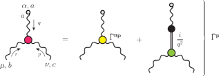
Figure 1: Three-gluon vertex $(BQ^{2})$ divided into one part that does not contain pole in $q^{2}$ and another that does. Analogous decomposition holds for the ghost-gluon vertex ($Bc\bar{c}$).

The cancellation of Eq. (5) can be evaded by introducing longitudinally coupled $1/q^{2}$ poles to the PT-BFM vertices cited above. For example, in Fig. 1, we illustrate the division of the three-gluon $BQ^{2}$ vertex into one part that does not contain pole in $q^{2}$ (yellow) and another that does (green). Similar decomposition holds for the ghost-gluon vertex, $Bc\bar{c}$. As we will see in what follows, such inclusion triggers the Schwinger mechanism, allowing the generation of a gauge boson mass.

In this presentation, we will consider the possibility of poles for both $BQ^{2}$ and $Bc\bar{c}$ vertices, then one has

$$\widetilde{\Gamma}_{\mu\alpha\beta}(q,r,p) =\widetilde{\Gamma}^{\mathrm{np}}_{\mu\alpha\beta}(q,r,p)+i\frac{q_{\mu}}{q^{2}}\widetilde{C}_{\alpha\beta}(q,r,p),$$

$$\widetilde{\Gamma}_{\mu}(q,r,p) =\widetilde{\Gamma}^{\mathrm{np}}_{\mu}(q,r,p)+i\frac{q_{\mu}}{q^{2}}\widetilde{C}_{\mathrm{gh}}(q,r,p),$$ (6)

where the superscript “np” stands for “no-pole” and $\widetilde{C}_{\alpha\beta}$ and $\widetilde{C}_{\mathrm{gh}}$ are the bound-state gluon-gluon and gluon-ghost wave functions, respectively. Then, to keep the symmetry of the theory intact, we require that the STIs of (3) preserve their form when including the poles, thus

$$q^{\mu}\widetilde{\Gamma}^{\mathrm{np}}_{\mu\alpha\beta}+\widetilde{C}_{\alpha\beta}=i\Delta_{\alpha\beta}^{-1}(r)-i\Delta_{\alpha\beta}^{-1}(p),$$

$$q^{\mu}\widetilde{\Gamma}^{\mathrm{np}}_{\mu}+\widetilde{C}_{\mathrm{gh}}=iD^{-1}(r^{2})-iD^{-1}(p^{2}).$$ (7)

where the vertices and the bound state wave functions are functions of $(q,r,p)$. We can now take the limit as $q\to 0$, so that the zeroth order terms in $q$ yields

$$\widetilde{C}_{\alpha\beta}(0,r,-r) =0; \widetilde{C}_{\mathrm{gh}}(0,r,-r) =0,$$ (8)

while the terms linear in $q$ provide a new set of WTIs,

$$\widetilde{\Gamma}^{\mathrm{np}}_{\mu\alpha\beta} =-i\frac{\partial}{\partial r^{\mu}}\Delta^{-1}_{\alpha\beta}(r)-\left\{\frac{\partial}{\partial q^{\mu}}\widetilde{C}_{\alpha\beta}(q,r,-r-q)\right\}_{q=0},$$

$$\widetilde{\Gamma}^{\mathrm{np}}_{\mu} =-i\frac{\partial}{\partial r^{\mu}}D^{-1}(r^{2})-\left\{\frac{\partial}{\partial q^{\mu}}\widetilde{C}_{\mathrm{gh}}(q,r,-r-q)\right\}_{q=0}.$$ (9)

The first terms on the r.h.s. of Eq. (9) lead to a result in the form of Eq. (5), so their contributions vanish. However, the second terms survive, from which we obtain Aguilar:2017dco .

$$\Delta^{-1}(0) =\lambda\int_{k}k^{2}\Delta^{2}(k^{2})\left[1-\frac{3}{2}g^{2}C_{A}Y(k^{2})\right]\widetilde{C}_{\mathrm{gl}}^{\prime}(k^{2})$$

$$-\frac{\lambda}{3}\int_{k}k^{2}D^{2}(k^{2})\widetilde{C}_{\mathrm{gh}}^{\prime}(k^{2})\,,$$ (10)

where $\lambda=3g^{2}C_{A}F(0)/2$ with $C_{A}$ being the Casimir eigenvalue of the adjoint representation and $\widetilde{C}_{\mathrm{gl}}$ is the form factor of the metric tensor $g_{\alpha\beta}$ in the tensorial decomposition of $\widetilde{C}_{\alpha\beta}$. Additionally, we defined

$$C_{i}^{\prime}(k^{2})=\lim_{q\to 0}\left\{\frac{\partial\widetilde{C}_{i}(q,k,-k-q)}{\partial(k+q)^{2}}\right\},\;\;i=\mathrm{gl},\mathrm{gh}.$$ (11)

From Eq. (10), we notice that, in order for $\Delta^{-1}(0)$ to acquire a nonvanishing value, we need at least one of $\widetilde{C}_{\mathrm{gl}}^{\prime}$ and $\widetilde{C}_{\mathrm{gh}}^{\prime}$ do not vanish identically. In addition, it is possible to establish a link between $\widetilde{C}_{\mathrm{gl}}^{\prime}$ and a running gluon mass through Aguilar:2017dco

$$m^{2}(q^{2})=\Delta^{-1}(0)+\int_{0}^{q^{2}}\!\!{\rm d}y\,\widetilde{C}_{\mathrm{gl}}^{\prime}(y)\,.$$ (12)

III Dynamics of massless pole formation

From the SDEs satisfied by the $BQ^{2}$ and $Bc\bar{c}$ vertices in the limit $q\rightarrow 0$, one can derive a system of integral equations that governs the behavior of $\widetilde{C}_{\mathrm{gl}}^{\prime}$ and $\widetilde{C}_{\mathrm{gh}}^{\prime}$ as shown in the Fig. 2. From Eq. (8), we know that the zeroth order terms vanish. Thus, the derivative terms will give the leading contributions. To proceed further with the derivation, we approximate the four-point kernels ${\mathcal{K}}_{i}$, appearing in the diagrams of the Fig. 2. to their lowest-order set of diagrams. In doing that we arrive at the following coupled system of equations Aguilar:2017dco

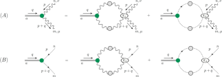
Figure 2: Coupled system of BSEs for the functions $\widetilde{C}_{\mu\nu}$ (top) and $\widetilde{C}_{\mathrm{gh}}$ (bottom).

$$\widetilde{C}_{\mathrm{gl}}^{\prime}(q^{2}) =\frac{8\pi}{3}\alpha_{s}C_{A}\!\left[\int_{k}\!\widetilde{C}_{\mathrm{gl}}^{\prime}(k^{2})\Delta^{2}(k)\Delta(k+q){\cal N}_{1}(k,q)+\frac{1}{4}\int_{k}\!\widetilde{C}_{\mathrm{gh}}^{\prime}(k^{2})D^{2}(k)D(k+q){\cal N}_{2}(k,q)\!\right]\!,$$

$$\widetilde{C}_{\mathrm{gh}}^{\prime}(q^{2}) =2\pi\alpha_{s}C_{A}\!\left[\int_{k}\!\widetilde{C}_{\mathrm{gl}}^{\prime}(k^{2})\Delta^{2}(k)D(k+q){\cal N}_{3}(k,q)+\frac{1}{2}\int_{k}\!\widetilde{C}_{\mathrm{gh}}^{\prime}(k^{2})D^{2}(k)\Delta(k+q){\cal N}_{4}(k,q)\!\right]\!,$$ (13)

with

$${\cal N}_{1}(k,q) =\frac{(q\!\cdot\!k)[q^{2}k^{2}-(q\!\cdot\!k)^{2}]}{q^{4}k^{2}(k+q)^{2}}f_{\mathrm{gl}}^{2}(k+q)$$

$$\times\left[8q^{2}k^{2}+6(q\!\cdot\!k)(q^{2}+k^{2})+3(q^{4}+k^{4})+(q\!\cdot\!k)^{2}\right],$$

$${\cal N}_{2}(k,q) =\frac{(q\!\cdot\!k)[q^{2}k^{2}-(q\!\cdot\!k)^{2}]}{q^{4}}f_{\mathrm{gh}}^{2}(k+q),$$

$${\cal N}_{3}(k,q) =\frac{(q\!\cdot\!k)[q^{2}k^{2}-(q\!\cdot\!k)^{2}]}{q^{2}k^{2}}f_{\mathrm{gh}}^{2}(k+q),$$

$${\cal N}_{4}(k,q) =\frac{(q\!\cdot\!k)[q^{2}k^{2}-(q\!\cdot\!k)^{2}]}{q^{2}(k+q)^{2}}f_{\mathrm{gh}}^{2}(k+q),$$ (14)

where the $f_{\mathrm{gl}}(r)$ and $f_{\mathrm{gh}}(r)$ are Ansätze employed for the three-gluon and ghost-gluon vertices. More specifically,

$$\Gamma_{\mu\alpha\beta}(q,r,p)=f_{\mathrm{gl}}(r)\Gamma^{(0)}_{\mu\alpha\beta}(q,r,p),$$

$$\Gamma_{\mu}(q,r,p)=f_{\mathrm{gh}}(r)\Gamma^{(0)}_{\mu}(q,r,p),$$ (15)

where $\Gamma^{(0)}$ is the tree-level expression for the vertices.

It is interesting to notice that, when we take the limit of $q\to 0$ in the Eq. (13), $\widetilde{C}_{\mathrm{gl}}(0)$ saturates to a constant Binosi:2017rwj , whereas the structure of the ${\cal N}_{3}$ and ${\cal N}_{4}$ kernels implies that $\widetilde{C}_{\mathrm{gh}}(0)=0$.

IV Numerical Analysis

To solve the BSE system given by Eq. (13), we have to specify the following four external functions: $\Delta(q)$, $F(q)$, and the form factors $f_{\mathrm{gl}}(q)$ and $f_{\mathrm{gh}}(q)$. For the propagators, we use fits for the $SU(3)$ lattice data of the Ref. Bogolubsky:2009dc , whereas for the form factors, we employ their expected nonperturbative behavior, in the symmetric configuration, derived either in the lattice or SDE analysis Athenodorou:2016oyh ; Boucaud:2017obn ; Binosi:2017rwj ; Aguilar:2013xqa .

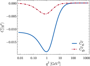
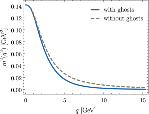
Figure 3: Normalized gluon and ghost solutions $\widetilde{C}_{\mathrm{gl}}^{\prime}(q^{2})$ and $\widetilde{C}_{\mathrm{gh}}^{\prime}(q^{2})$ of the BSE system given by Eqs (13). Dynamical gluon mass obtained in this study, compared to the one attained in the absence of ghosts.

Using the quantities specified above, we have solved the coupled system of BSEs (13). In the left panel of the Fig. 3, we show the normalized solution for $\widetilde{C}_{\mathrm{gl}}^{\prime}(q^{2})$ and $\widetilde{C}_{\mathrm{gh}}^{\prime}(q^{2})$ obtained for $\alpha_{s}=0.43$. In the right panel, the blue continuous line represents the resulting gluon mass obtained with Eq. (12), while the gray dashed curve is the same quantity obtained in the absence of the ghost poles, i.e. we set in the Eq (13) $\widetilde{C}_{\mathrm{gh}}^{\prime}(q^{2})=0$ Binosi:2017rwj . From Fig. 3, clearly we notice that the presence of ghosts implies a faster running of the gluon mass. Additionally, one can see that the gluon mass, shown in the right panel of Fig. 3, can be fitted using the following power-law behavior Aguilar:2014tka

$$m^{2}(q^{2})=m^{2}(0)/[1+(q^{2}/m_{1}^{2})^{1+p}],$$ (16)

where $m_{1}=0.37$ GeV and $p=0.24$ (blue continuous) as opposed to $m_{1}=0.36$ GeV and $p=0.1$, which represents the case where the effects of the ghosts were neglected (gray dashed).

V Conclusions

Within the PT-BFM scheme, we derived the BSE system which describes the dynamics of massless poles formation in the $BQ^{2}$ and $Bc\bar{c}$ vertices. By solving this system, we were able to obtain non-trivial solutions for both $\widetilde{C}_{\mathrm{gl}}^{\prime}(q^{2})$ and $\widetilde{C}_{\mathrm{gh}}^{\prime}(q^{2})$, which indicates that the dynamics of QCD is indeed strong enough to generate such poles.

Then, from the numerical results, we conclude that the contribution associated with the pole of the gluon-ghost vertex is suppressed when compared to that coming from the three-gluon vertex. The main effect of the presence of ghosts was observed to be a slight modification in the running of the gluon mass.

- (1) I. C. Cloet and C. D. Roberts, Prog. Part. Nucl. Phys. 77, 1 (2014).
- (2) A. C. Aguilar, D. Binosi, and J. Papavassiliou, Front. Phys.(Beijing) 11, 111203 (2016).
- (3) C. D. Roberts, Few Body Syst. 58, 5 (2017).
- (4) A. Cucchieri and T. Mendes, PoS LAT2007, 297 (2007).
- (5) A. Cucchieri and T. Mendes, Phys.Rev.Lett. 100, 241601 (2008).
- (6) A. Cucchieri and T. Mendes, Phys.Rev. D81, 016005 (2010).
- (7) P. O. Bowman et al., Phys. Rev. D76, 094505 (2007).
- (8) I. Bogolubsky, E. Ilgenfritz, M. Muller-Preussker, and A. Sternbeck, Phys. Lett. B676, 69 (2009).
- (9) O. Oliveira and P. Silva, PoS LAT2009, 226 (2009).
- (10) A. Ayala, A. Bashir, D. Binosi, M. Cristoforetti, and J. Rodriguez-Quintero, Phys. Rev. D86, 074512 (2012).
- (11) P. Bicudo, D. Binosi, N. Cardoso, O. Oliveira, and P. J. Silva, Phys. Rev. D92, 114514 (2015).
- (12) J. M. Cornwall, Phys. Rev. D26, 1453 (1982).
- (13) A. C. Aguilar and J. Papavassiliou, JHEP 0612, 012 (2006).
- (14) A. C. Aguilar, D. Binosi, and J. Papavassiliou, Phys. Rev. D78, 025010 (2008).
- (15) A. C. Aguilar, D. Ibanez, V. Mathieu, and J. Papavassiliou, Phys.Rev. D85, 014018 (2012).
- (16) D. Ibañez and J. Papavassiliou, Phys.Rev. D87, 034008 (2013).
- (17) A. C. Aguilar, D. Binosi, C. T. Figueiredo, and J. Papavassiliou, (2016).
- (18) D. Binosi and J. Papavassiliou, J.Phys.G G30, 203 (2004).
- (19) D. Binosi and J. Papavassiliou, Phys.Rev. D77, 061702 (2008).
- (20) D. Binosi and J. Papavassiliou, JHEP 0811, 063 (2008).
- (21) J. S. Schwinger, Phys. Rev. 125, 397 (1962).
- (22) J. S. Schwinger, Phys. Rev. 128, 2425 (1962).
- (23) A. C. Aguilar and J. Papavassiliou, Eur.Phys.J. A35, 189 (2008).
- (24) A. C. Aguilar, D. Binosi, C. T. Figueiredo, and J. Papavassiliou, Eur. Phys. J. C78, 181 (2018).
- (25) R. Jackiw and K. Johnson, Phys. Rev. D8, 2386 (1973).
- (26) J. M. Cornwall and R. E. Norton, Phys. Rev. D8, 3338 (1973).
- (27) R. Jackiw, In *Erice 1973, Proceedings, Laws Of Hadronic Matter*, New York 1975, 225-251 and M I T Cambridge - COO-3069-190 (73,REC.AUG 74) 23p (1973).
- (28) D. Binosi and J. Papavassiliou, Phys. Rept. 479, 1 (2009).
- (29) D. Binosi, L. Chang, J. Papavassiliou, and C. D. Roberts, Phys.Lett. B742, 183 (2015).
- (30) A. C. Aguilar, D. Binosi, J. Papavassiliou, and J. Rodriguez-Quintero, Phys. Rev. D80, 085018 (2009).
- (31) D. Binosi and J. Papavassiliou, Phys. Rev. D97, 054029 (2018).
- (32) A. Athenodorou et al., Phys. Lett. B761, 444 (2016).
- (33) P. Boucaud, F. De Soto, J. Rodríguez-Quintero, and S. Zafeiropoulos, Phys. Rev. D95, 114503 (2017).
- (34) A. C. Aguilar, D. Ibañez, and J. Papavassiliou, Phys. Rev. D87, 114020 (2013).
- (35) A. C. Aguilar, D. Binosi, and J. Papavassiliou, Phys. Rev. D89, 085032 (2014).