Intrinsic Image Transformation via Scale Space Decomposition

Abstract

We introduce a new network structure for decomposing an image into its intrinsic albedo and shading. We treat this as an image-to-image transformation problem and explore the scale space of the input and output. By expanding the output images (albedo and shading) into their Laplacian pyramid components, we develop a multi-channel network structure that learns the image-to-image transformation function in successive frequency bands in parallel, within each channel is a fully convolutional neural network with skip connections. This network structure is general and extensible, and has demonstrated excellent performance on the intrinsic image decomposition problem. We evaluate the network on two benchmark datasets: the MPI-Sintel dataset and the MIT Intrinsic Images dataset. Both quantitative and qualitative results show our model delivers a clear progression over state-of-the-art.

1 Introduction

There has been an emerging trend in representation learning that learns to disentangle from an image latent codes accounting for the various dimensions of the input, e.g., illumination, pose, and attributes [2, 43, 47]. Yet one of the preliminary forms of this problem – to decompose an image into its intrinsic albedo and shading – has drawn less attention. Solutions to the intrinsic image decomposition problem would enable material editing, provide cues for depth estimation, and provide a computational explanation to the long standing lightness constancy problem in perception. However, even with exciting progress (e.g. [8, 25]), this problem still remains a challenging task for continuing effort.

Part of the difficulty arises from the under-determinedness of this problem. Based on prior knowledge of albedo and shading, the Retinex algorithm constrains the decomposition into a thresholding problem in the gradient domain. This model is practical, but would fail to handle complex material or geometry that has sharp edges or casts shadows under strong point sources. Another part of the difficulty lies in the complexity of the forward image generation process – a process that transforms scene material, geometry and illumination into a 2D image via the dynamics of optical interactions and projection. Intrinsic image decomposition is partly trying to invert this process.

\begin{overpic}[width=433.62pt,clip,trim=0.0pt 853.18748pt 1455.43748pt 0.0pt]{illustration2.pdf}\end{overpic}

Figure 1: Given an input image, our lapPyrNet jointly produces Laplacian pyramid components that collapse into the target albedo and shading images in high quality. Our network features by a multi-channel architecture that treats intrinsic image decomposition as image-to-image transformation in separate frequency bands in the scale space.

In this work, we treat the intrinsic image decomposition process in an image-to-image transformation framework, using a deep neural network as a function approximator to learn the mapping relations. While models of similar ideas have been proposed (e.g. [37, 32]), our model explores the scale space of the network input and output, and considers to simply the transformation as a whole by horizontally expanding the functor approximation pipeline into a parallel set of sub-band transformations.

The contribution of this work is in developing a scale-space decomposition network for intrinsic image generation. We do this by resuing the classical Gaussian and Laplacian pyramid structure with learnable down/up samplers. The result is a multi-branch network that produces a level-of-detail decomposition of the output albedo and shading; each decomposition component is predicted by one sub-network, which is aggregated together to match the target (Figure 1). We propose novel loss functions that respect the distinctive properties of albedo and shading for edge preservation and smoothness, respectively. We further implement a data augmentation scheme to fight against the scarcity of labeled data – that is, we take inspiration from breeder learning [36], and use a preliminarily trained network to generate predictions from unlabeled images, and a synthesis procedure to perturb and generate new data with exact ground truth labels for iterative model refinement. This data augmentation scheme is applicable to other network training that learns to invert a generative process.

We have evaluated our model on the MPI-Sintel dataset [7] and the MIT intrinsic image dataset [17]. Experimental results demonstrate the effectiveness of the proposed model and our network engineering components. Our final model achieves state-of-the-art performance with a significant margin over previous methods in a variety of evaluation metrics.

2 Related work

Intrinsic images: A series of solutions have been seen since Barrow and Tenenbaum first propose this problem [46], for example, the Retinex method [29, 18], learning based method using local texture and color cues [45], and joint optimization using data-driven priors [4]. With the advent of deep neural networks, solution to this problem has shifted to a pure data-driven, end-to-end training with various forms of feed forward convolutional neural networks. Direct Intrinsics [37] is a successful early example of this type, using a (back then seemingly bold) multi-layer CNN architecture to transform an image directly into shading and albedo. Successive models include the work of Kim et al. [25] that predicts depth and the other intrinsic components together with a joint convolutional network that has shared intermediate layers and a joint CRF loss, and the DARN [32] network that incorporates a discriminator network and the adversarial training scheme to enhance of the performance of a “generator” network that produces the decomposition results.

Image scale space and pyramid structures: The investigation of image scale space is no less old-fashioned than that of the intrinsic image decomposition in vision. The studies of Koenderink [27] in the 1980’s reveals a diffusion process that “explicitly defines the deep structure of (an) image” that relates to the DOG structure revealed in even earlier studies [35]. Around the same time, Burt and Adelson proposed the Laplacian pyramid structure that decomposes an image into a hierarchical Level-Of-Detail (LOD) representation using successive Gaussian filtering and the DOG operator [6]. Scale space decomposition also widely exists in other fields of study, such as 3D graphics (e.g. [19]) and numerical computing (e.g. [48]).

Deep convolutional networks provide a natural hierarchical feature pyramid for multi-scale information processing. The feature pyramid network (FPN) makes predictions from multi-level feature maps for object detection with top-down communication [34]. Pinheiro et al. [40] propose a two-way hierarchical feature aggregation network for object segmentation. The work of Ghiasi et al. [16] produces segmentation score maps with spatia-semantic trade-offs from different network layers, and aggregates them into a final segmentation map by pyramid collapsing. The work of Lai et al. [28] utilizes a similarly deeply stacked network and feature maps to generate image detail map of multi-scales for image super-resolution. Notably, all of the above work utilizes hierarchical features from a CNN network for multi-scale processing. In generative modeling, a Laplacian pyramid inspired GAN network is proposed by Denton et al. [11] that learns generative modules in a Laplacian pyramid structure for image generation.

Image-to-image transformation: There is a variety of vision tasks that can be formulated as image-to-image transformation problem. Intrinsic image decomposition is one such example. Isola et al. [23] recently introduced an image-to-image translation network for several other tasks, including image colorization, sketch-to-image, and image-to-map generation. In this work, Isola et al. model the image-to-image transformation as a conditional generative process and use an adversarial loss for network training.

Note that a set of other vision tasks, such as dense pixel labeling (e.g. object segmentation [1]), depth estimation from single image [49], and the recent label-to-image synthesis network ([9], also in [23]) can also be framed as the image-to-image transformation problem, that is, to map pixels to pixels. Instead of hand engineering the mapping process for each task individually, we engineered a generic, extensible network architecture that is tangential to the work of Isola et al. [23] and features in exploiting the dimension of scale-space decomposition for the form of input/output transformation of this problem.

3 Method

Let us first consider the transformation of an input image $I$ to an output image $A$ as a complex, highly nonlinear, and pixel-wise nonlocal mapping function $I\rightarrow f(I)$. It has been well demonstrated that deep convolutional neural networks are a general and practical parametrization and optimization framework for a variety of such mapping relations (from image classification to image-to-language translation). Now, let us consider how to adapt the network architecture to the image-to-image transformation problem, in which the input and output are both images that have a natural Level-Of-Detail (LOD) pyramid structure, and that the mapping function linking the input to the output may also have a multi-channel decomposition based on the pyramid hierarchy. In the next section (3.1) we are going to describe our model reformation process from a ResNet architecture that exploits this property to our final multi-channel hierarchical network architecture.

We write the Gaussian pyramid of an image $I$ as $[I_{0},I_{1},...,I_{K}]$, where $I_{0}=I$ and $K$ is the total number of layers. We denote the $k$-th Laplacian pyramid layer by $\mathcal{L}_{k}(I)=I_{k}-u(I_{k+1})$ where $u$ is the up-sample operator. By definition, the Laplacian pyramid expansion of the image is $I=[\mathcal{L}_{0}(I),\mathcal{L}_{1}(I),...,\mathcal{L}_{k-1}(I),I_{K}]$, where $\mathcal{L}_{0}(I)$ is the detail layer of the original resolution and $I_{K}$ is the lowest resolution layer defined in the Gaussian pyramid.

\begin{overpic}[width=433.62pt,clip,trim=15.05624pt 0.0pt 142.53249pt 0.0pt]{reformation.pdf}\end{overpic}

Figure 2: Network architecture reformation (see section 3.1).

3.1 Network Architecture and Reformation

First, let us use a simplified network of two blocks ($L$ and $H$) to model the mapping $I\rightarrow f(I)$: $L$ for the mapping of the low frequency band, and $H$ handles the mapping in the high frequency band and whatever residuals that are left out by $L$. With the skip connection and summation of the output of $L$ to the output of $H$, this network (Figure 2-a) is an instantiation of the ResNet architecture [21].

Next, by applying Laplacian pyramid expansion on the output, we can split the loss for (a) into two components: the output of $L$ is restrained to fit the low-frequency Gaussian component, and that of $H$ to fit the Laplacian detail component separately (Figure 2-b). This reformed network is equivalent to (a) but with tighter constraints.

A critical transition is from (b) to (c) – as it turns out to be possible to re-wire the two stacked blocks into two parallel branches, by connecting the output of $L$ to that of $H$ with summation, and adjusting the loss on $H$ accordingly. The resulted network structure (c) is equivalent to (b) – they represent two equivalent forms of the Laplacian decomposition equation, i.e., by moving the residual component from lhs to rhs and change the sign. The loss of $L$ in (c) remains the same as a regularizer and our experiments find it is optional and is a barrier for numerical performance. The network structure (c) is the building block for our final extended model.

The final extended model is illustrated in Figure 2-d, for which we introduce multiple sub-network blocks $H_{0},H_{1},...H_{K-1}$ for the high frequency bands and one subnetwork block $L_{K}$ for the low frequency, in analogy to the Laplacian pyramid decomposition structure: the inputs to the network blocks are down-sampled in cascade, and outputs of the network blocks are up-sampled and aggregated from left to right to form the target output. All of the parameters of the down-sample and up-sample operators (the gray-shaded trapezoids in Figure 2) are learned in network. All of the network blocks share the same architectural topology, which we refer as “residual blocks” and describe in detail in section 3.2.

3.2 Residual Block

The residual blocks are end-to-end convolutional subnetworks that share the same topology, and transform the input in different scales to the corresponding Laplacian pyramid components. Each residual block consists of 6 sequentially concatenated Conv(3x3)-ELU-Conv(3x3)-ELU sub-structures (Figure 3 (a-b)). Because we are predicting per-pixel value from an input image, no fully connected layers are used. We adopt the skip connection scheme that is popular in recent researches (e.g.  [21],  [34]), including some variant of the DenseNet architecture by Huang et al. [22]. Specifically, in each sub-structure, the output of the last Conv is element-wise accumulated with a skip connection, and the result is the input to the last ELU unit. The intermediate layers have 32 feature channels and output is a 3-channel image or residual image. A 1x1 Conv is added to the skip connection path of the first and last layer for dimension expansion/reduction to match the output of the residual path (Figure 3 (c)).

Instead of ReLU and Batch Normalization, we use Exponential Linear Units (ELU) as our activation function [10], because ELU can generate negative activation value when $x<0$ and has zero-mean activations, both of which improve the robustness to noise and convergence in training when our network becomes deeper. Besides, we removed the BN layer because it can be partially replaced by ELU which is 2x faster and more memory efficient.

\begin{overpic}[width=433.62pt,clip]{block.pdf}\end{overpic}

Figure 3: Illustration of our Residual Block

3.3 Loss Function

The loss function is defined as follows:

$$\mathcal{L}=\lambda_{d}\mathcal{L}_{data}+\lambda_{p}\mathcal{L}_{percep}+\lambda_{t}\mathcal{L}_{tv}$$ (1)

which contains a Data loss, a feature-based Perceptual loss and a Total Variation loss as regularization. The hyper parameters are empirically set as: $\lambda_{d}$ = 1.0; $\lambda_{p}$ =0.5; $\lambda_{t}=10^{-4}$.

Data loss: The data loss defines pixel level similarity between the predicted image and the ground-truth. Instead of using the pixel-wise MSE, we employ the following joint bilateral filtering (also known as cross bilateral filtering[13, 39]) loss combined with the constraint that the multiplication of the predicted albedo and shading should match the input:

$$\mathcal{L}_{data}=\sum\limits_{\mathcal{C}\in\{A,S\}}\frac{1}{N_{p}}\sum\limits_{p\in\mathcal{C}}||{\mathcal{J}_{p}}-C_{p}||_{2}^{2}+||\widetilde{A}\!*\!\widetilde{S}\!-\!{I}||_{2}^{2}$$ (2)

$$\mathcal{J}_{p}=\frac{1}{\mathcal{W}_{p}}\sum\limits_{q\in\mathcal{N}(p)}G_{\sigma_{s}}(||p-q||)G_{\sigma_{r}}(|\mathcal{C}_{p}-\mathcal{C}_{q}|)\widetilde{\mathcal{C}}_{p}$$ (3)

$$\mathcal{W}_{p}=\sum\limits_{q\in\mathcal{N}(p)}G_{\sigma_{s}}(||p-q||)G_{\sigma_{r}}(|{\mathcal{C}}_{p}-\mathcal{C}_{q}|)$$ (4)

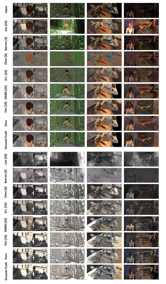
Figure 6: Qualitative results on four examples of the MPI-Sintel benchmark dataset and comparison to previous methods (results are excerpted from paper with limited resolution). Notice our decomposition results exhibit good edge preserving property and are visually close to the ground truth.

The cross bilateral filtering loss ensures smoothness of the output albedo and shading, and preserves sharp edges for albedo and strong cast shadows in shading (e.g. Figure 1). In contrary, the alternative MSE loss tends to produce blurry edges across boundaries in the output, which is also seen in [37] and [32] (see Figure 6). Here $\sigma_{s}$ = 1.0, $\sigma_{r}$ uses the adaptive bilateral filtering mechanism, $G_{\sigma_{s}}$ and $G_{\sigma_{r}}$ are the spatial and range Gaussian kernels, both with neighborhood size 5x5.

Perceptual loss: High-level semantic structures should be preserved in the transformation process as well, so a CNN-feature based perceptual loss [24, 12] is used. We make use of the standard VGG-19 [44] network to extract semantic information from neuron activations. Our perceptual loss is defined as follows:

$$\mathcal{L}_{feat}=\sum\limits_{\mathcal{C}\in\{A,S\}}\sum\limits_{l}\frac{1}{F_{l}H_{l}W_{l}}||\Phi_{l}(\widetilde{\mathcal{C}})-\Phi_{l}(\mathcal{C})||_{2}^{2}$$ (5)

where $\Phi_{l}(\mathcal{C})$ is the network activations of $C$ at the $l$-th layer that have size $F_{l}\times H_{l}\times W_{l}$, and $l=relu1\_2,relu2\_2,relu3\_4$ and $relu4\_4$ are the VGG-19 network layers before pooling.

Total Variation loss: Lastly, we use a total variation term to impose smoothness of the output results.

$$\mathcal{L}_{tv}=\sum\limits_{\mathcal{C}\in\{A,S\}}\sum\limits_{i,j}|\widetilde{\mathcal{C}}_{i+i,j}-\widetilde{\mathcal{C}}_{i,j}|+|\widetilde{\mathcal{C}}_{i,j+1}-\widetilde{\mathcal{C}}_{i,j}|$$ (6)

where $i$ and $j$ are image row and column indices.

Our final model is trained with the above loss on the output of $H_{0}$ combined with all outputs from lower level branches (Figure 2-(d)). This constrains all network channels simultaneously and gradients can back-propagate and dispatch more flexibly. Another training scheme, as we mentioned in section 3.1, is to train the network from left to right in an incremental manner ($L_{K}$, $H_{K-1}$, $H_{K-2}$, …), and every time has the loss defined for the corresponding Gaussian pyramid level, e.g. $loss(A_{K},\widetilde{A}_{K})$, $loss(A_{K-1},\widetilde{A}_{K-1})$, $loss(A_{0},...\widetilde{A}_{0})$ for the albedo network. This incremental training constrains the network to output a near-perfect Gaussian pyramid, and that the sub-network $H_{i},i=K-1,...0$ outputs the expected Laplacian detail layer. Figure 1 shows intermediate outputs of the network trained in this scheme for illustration. Except we state otherwise, the quantitative results are obtained using the simultaneous training scheme.

3.4 Self-Augmented Training

In this section, we describe a data augmentation strategy for incorporating unlabeled images to self-augment our network training process. We draw the inspiration from the work of breeder learning [36]. The idea is to employ a forward generative model to generate new training pairs for a model by perturbing parameters produced by the model to be augmented. This mechanism bears the spirit of Boostrap to some extent and turns out to be quite effective. For example, Li et al. [33] recently applied this strategy in an appearance modeling network by generating training images from model’s predicted reflectance of unlabeled images.

We start with a preliminary network trained with a moderately sized dataset that has ground-truth albedo and shading. We then apply the network to a set of new images and obtain the estimated albedo $\tilde{A}$ and shading $\tilde{S}$. With a straightforward synthesis procedure, we can generate a new image from the estimations. Note that by our loss definitions, $\tilde{A}$ and $\tilde{S}$ are not hard constrained to exactly match the input image (as in [32]), so the new synthesized images will deviate from the original ones.

To introduce further perturbation in the augmented dataset, we additionally apply an Adaptive Manifold Filtering (AMF,  [15]) operation to $\tilde{A}$ and $\tilde{S}$ and use the filtered results to synthesize new data (see Figure 4). The AMF filtering operator suppresses noise or unwanted details in $\tilde{A}$ and $\tilde{S}$ that may come from the input images or produced by the premature network, and serves to “regularize” the manifold of the new synthesized images and their ground-truth label space so that the network is not misled to overfit capricious details in the self-augmented training process.

\begin{overpic}[width=433.62pt,clip]{refine.pdf}\end{overpic}

Figure 4: Our data augmentation process uses a preliminarily train model to produce estimations for unlabeled data, and use the estimation result to synthesize new data for self-augmented training.

4 Evaluation

In this section we describe evaluation of the model on the MPI-Sintel dataset and the MIT Intrinsic Images dataset and show results in Table 1-3 and Figure 5-6.

4.1 Experiment Setup

DataSet and Metrics The MPI-Sintel dataset[7] is composed of 18 scene level computer generated image sequences, 17 of which contain 50 images of the scene and one contains 40 images. We follow [37, 32] and use the $ResynthSintel$ version in our experiment because the data satisfies the $\mathcal{A}\times\mathcal{S}=\mathcal{I}$ constraint. Two types of train/test split (scene split and image split) are used for head-to-head comparison with previous work. The scene split splits the dataset at scene level which takes half of the scenes for training and the rest scenes for testing. The image split randomly pick half of the images for training/testing without considering their scene category. The original version of the MIT Intrinsic dataset [17] has 20 object-level images taking in a laboratory environment setup, each with 11 different lighting conditions. We use the same strategy of [5] to split the data for direct comparison.

Evaluations are based on the following metrics:

si-MSE

scale-invariant mean squared error (si-MSE) defines the pixel-wise MSE up to a free scaling factor (see [5]).

si-LMSE

scale invariant local mean square error (si-LMSE) measures the averaged si-MSE on local window patches as the window slides over the image with a stride. The window size is usually set to 10% of the image size along the larger dimension and stride is half of the window size:

$$\text{si-LMSE}(\mathcal{C}_{gt},\widetilde{\mathcal{C}})=\frac{1}{N_{\mathcal{W}}}\sum_{\omega\in\mathcal{W}}\text{si-MSE}(\mathcal{C}_{gt}^{\omega},\widetilde{\mathcal{C}}^{\omega})$$

LMSE

The LMSE measure is the “normalized” si-LMSE measure on albedo and shading together. We use this metric on the MIT Intrinsic Images dataset. Local window size for si-LMSE is set to 20 (as in [18]):

$$\text{LMSE}=\frac{1}{2}\frac{\text{si-LMSE}(\mathcal{S}_{gt},\widetilde{\mathcal{S}})}{\text{si-LMSE}(\mathcal{S}_{gt},0)}+\frac{1}{2}\frac{\text{si-LMSE}(\mathcal{A}_{gt},\widetilde{\mathcal{A}})}{\text{si-LMSE}(\mathcal{A}_{gt},0)}$$

DSSIM

The structural similarity is quantized by dissimilarity structural similarity index measure as $\frac{1-\text{SSIM}}{2}$ (see [51] for SSIM definition).

Implementation Details We implemented our model in the PyTorch framework with mini-batch size 8. In training, we get the input image by randomly cropping patches of size 256 $\times$ 256 after scaling by a random factor in [0.8,1.2] and using random horizontal flipping with probability 0.5. We empirically construct 4 levels of pyramids and initialize all the weights with the strategy of [20]. Besides, we adopt the Adam [26] optimization method with a learning rate starting at $10^{-4}$ and decreasing to $10^{-6}$. We use 2x the size of the training data as the size of the augmentation data in both experiments.

Sintel image split	si-MSE			si-LMSE			DSSIM
	A	S	avg	A	S	avg	A	S	avg
Baseline: Constant Shading	5.31	4.88	5.10	3.26	2.84	3.05	21.40	20.60	21.00
Baseline: Constant Albedo	3.69	3.78	3.74	2.40	3.03	2.72	22.80	18.70	20.75
Color Retinex [18]	6.06	7.27	6.67	3.66	4.19	3.93	22.70	24.00	23.35
Lee et al. [30]	4.63	5.07	4.85	2.24	1.92	2.08	19.90	17.70	18.80
Barron & Malik [5]	4.20	4.36	4.28	2.98	2.64	2.81	21.00	20.60	20.80
Chen and Koltun [8]	3.07	2.77	2.92	1.85	1.90	1.88	19.60	16.50	18.05
Direct Intrinsic [38]	1.00	0.92	0.96	0.83	0.85	0.84	20.14	15.05	17.60
DARN [31]	1.24	1.28	1.26	0.69	0.70	0.70	12.63	12.13	12.38
Kim et al. [25]	0.7	0.9	0.7	0.6	0.7	0.7	9.2	10.1	9.7
Fan et al. [14]	0.67	0.60	0.63	0.41	0.42	0.41	10.50	7.83	9.16
Ours Sequential	0.83	0.74	0.79	0.58	0.54	0.56	7.61	7.91	7.76
Ours Hierarchical	0.81	0.78	0.79	0.58	0.58	0.58	8.18	7.16	7.62
Ours w/o Pyramid	0.92	1.37	1.15	0.65	1.15	0.90	8.44	10.96	9.70
Ours w/ MSE loss	0.72	0.62	0.67	0.62	0.46	0.50	7.98	6.37	7.18
Ours w/ ‘FPN’ input	0.73	0.60	0.67	0.49	0.43	0.46	6.84	6.76	6.80
Ours Final*	0.66	0.60	0.63	0.44	0.42	0.43	6.56	6.37	6.47
Ours Final+DA	0.61	0.57	0.59	0.41	0.39	0.40	5.86	5.97	5.92

Table 1: Quantitative Evaluation ($\times$100) on the MPI-Sintel image split

Sintel scene split	si-MSE			si-LMSE			DSSIM
	A	S	avg	A	S	avg	A	S	avg
Direct Intrinsic [38]	2.01	2.24	2.13	1.31	1.48	1.39	20.73	15.94	18.33
DARN [31]	1.77	1.84	1.81	0.98	0.95	0.97	14.21	14.05	14.13
Fan et al. [14]	1.81	1.75	1.78	1.22	1.18	1.20	16.74	13.82	15.28
Ours Sequential	1.61	1.56	1.58	1.05	1.11	1.08	10.24	11.90	11.07
Ours Hierarchical	1.59	1.51	1.55	0.98	1.01	0.99	8.70	9.55	9.13
Ours w/o Pyramid	1.82	2.01	1.92	1.01	1.39	1.20	14.43	14.27	14.35
Ours w/ MSE loss	1.47	1.44	1.46	0.92	0.95	0.93	9.48	10.97	10.23
Ours w/ ‘FPN’ input	1.46	1.40	1.43	0.96	0.97	0.97	8.50	9.30	8.90
Our Final*	1.38	1.38	1.38	0.92	0.93	0.92	8.46	9.26	8.86
Our Final+DA	1.33	1.36	1.35	0.82	0.89	0.85	7.70	8.66	8.18

Table 2: Quantitative Evaluation ($\times$100) on the MPI-Sintel scene split

4.2 Evaluation on MPI-Sintel Dataset

The evaluation results on the MPI-Sintel dataset are in Table 1-2 and Figure 6. Again, our model produces favorable results over previous methods, especially in the scene split where the network is less prone to “overfit” for the test data.

Comparison with Previous Work: We first compare our model with a series of previous methods, including the two naive baselines Constant Shading and Constant Albedo, a few of the traditional methods ([18, 30, 8, 5]), and the recent up-to-date neural network based models ([38, 31, 25, 14]). The result shows our model with/without data augmentation both yield new state-of-the-art performance across all the three metrics.

We do want to point out the quantitative result of all methods (including ours) on the Sintel image split might be misleading to some extent. This is because the image sequences of the same scene category in the Sintel dataset are very similar to each other, so by splitting all the data at image level (images of the same scene type may appear in both train and test sets), an over-fit network on the training set will still appear to “perform” well on the test set. But the scene split dataset will not have this problem. An interesting result in the Tables is that the margin of our results to previous results is larger in the scene split (Table 2) than the image split (Table 1). In the Tables, even though we hold a fairly moderate margin on the image split, the margin we hold on the scene split is up to $25\%$ in si-MSE and $43\%$ in DSSIM, showing that our network can generalize significantly better for this more challenging data split.

From Sequential to Parallel Architecture: An important network architecture reformation we described in section 3.1 is from the sequential structure to the multi-branch parallel structure (Figure 2-(a) to (c)). This reformation flattens a deeply stacked network into a set of parallel channels, therefore alleviates the issues of gradient back-propagation. The row (Ours Sequential) displays the result by the sequential architecture (a) in Figure 2. It shows this architecture produces comparable performance against previous works, but suboptimal to our final model, especially in the DSSIM metric (7.76 and 11.07 down to 6.47 and 8.86).

Hierarchical Optimization vs Joint Optimization: Another architectural optimization in our work is removing the constraint (loss) at each Laplacian pyramid level (Figure 2-(c)), and simultaneously train all the network channels with a single loss constraint (Figure 2-(d)). We call the optimization scheme in the latter case joint optimization, and that of the former hierarchical optimization. A figure is included in the supplemental material explaining more details of the hierarchical optimization. In Table 1-2, it shows a $10\%-15\%$ improvement by the joint optimization scheme across all metrics.

Self-Comparison on other Factors: We also have a set of controlled self-comparison with respect to other factors, including the pyramid structure, loss function, alternating network input, and data augmentation.
Pyramid structure The row (Ours w/o Pyramid) displays result using a single-channel network, i.e. we use a single residual block to produce output from input directly without having the multi-band decomposition structure. The results in Table 1 and Table 2 show that our counterpart model with the pyramid structure improves over than 30% compared to controlled setting by turning this feature off. Note the network complexity grows sub-linearly up to a constant factor as the number of pyramid layer increases.
Loss function: The row (Ours w/ MSE loss) displays result by replacing our loss function with the classical MSE loss. It turns out the quantitative error with the MSE loss does not degrade by a large factor in the scale-invariant MSE metrics. However, qualitative results in supplemental material do reveal the MSE loss produces results with blurry edges. The structure-based metric (DSSIM) also shows a clearer margin (from 10.23 to 8.86 in the scene split) between the MSE loss and our loss.
CNN features as input We further investigate the affect of having Gaussian pyramid image components as input of our network in this task, as most existing multi-scale deep networks (e.g. [34, 40, 16, 28]) use multi-scale features produced by a CNN network. The row (Ours w/ ‘FPN’ input) shows the result that takes CNN features as input following exactly the FPN network [34]. The comparison shows our final model holds a slight but unclear advantage, meaning that the high level features of a CNN still well preserve much of the necessary semantic information for our pixel-to-pixel transformation network.
Data augmentation The last row in Table 1-2 shows the effect of our data augmentation. We obtain a set of cartoon clips crawled from the Web that share similar property with the MPI dataset (see an example in Figure 4). The size of the augmentation data is set to 2 times of the labeled training data. Further increasing the augmentation data size did not produce important improvement in our experiment.

4.3 Evaluation on MIT Intrinsic Images Dataset

We also evaluated the performance of our model against a set of previous methods on the MIT Intrinsic Images dataset. The results are shown in Table 3 and Figure 5. In this set of experiments, we conducted data augmentation in two different setups: Ours + DA and Ours + $\text{DA}^{+}$. The difference is in the data that we take for the augmentation. Ours + DA is by the ordinary setting where the augmenting data is searched from the web by a set of similar object category names the dataset provides. In Ours + $\text{DA}^{+}$, instead, we generate the augmenting dataset from the same set of objects (depth and reflectance) of the MIT Intrinsic Images dataset under new illumination conditions (spherical harmonic illuminations from [3] and the rendering method by [41]). This creates a dataset that highly resembles the original dataset and is practically impossible to acquire in real case. In other words, it sets a ceiling for the quality of augmentation data. The results in Table 3 shows that both augmentation setups are effective, and the latter one gives clue to the limit we can get from the data augmentation scheme we introduced for this task.

Figure 5: Qualitative results on the MIT Intrinsic dataset examples. Top three rows are albedo; the bottom three rows are shading.

Mit Intrinsic Data	si-MSE			LMSE
	Albedo	Shading	Average	Total
Zhou et al. [50]	0.0252	0.0229	0.0240	0.0319
Barron et al. [5]	0.0064	0.0098	0.0081	0.0125
Shi et al. [42]	0.0216	0.0135	0.0175	0.0271
Direct Intrinsic et al. [38]	0.0207	0.0124	0.0165	0.0239
Fan et al. [14]	0.0127	0.0085	0.0106	0.0200
Ours*	0.0089	0.0073	0.0081	0.0141
Ours + DA	0.0085	0.0064	0.0075	0.0133
Ours + $\text{DA}^{+}$	0.0074	0.0061	0.0068	0.0121

Table 3: Evaluation on the MIT Intrinsic Images dataset.

5 Conclusion

We have introduced a Laplacian pyramid inspired neural network architecture for intrinsic images decomposition. The network models the problem as image-to-image transformation and expands the input and output in their scale space. We have conducted experiments on the MPI Sintel and MIT dataset and produced state-of-the-art quantitative results and good qualitative results. For future work, we expect the proposed network architecture to be tested and refined on other image-to-image transformation problems, e.g., pixel labeling or depth regression.

Acknowledgment We thank all the anonymous reviewers. This work is supported in part by National Key R$\&$D Program of China (No. 2017YFB1002703), by NSFC (No. 61602406), by ZJNSF (No. Q15F020006), and by a special fund from the Alibaba - ZJU Joint Institute of Frontier Technologies.

References

- [1] M. Amirul Islam, M. Rochan, N. D. B. Bruce, and Y. Wang. Gated feedback refinement network for dense image labeling. In The IEEE Conference on Computer Vision and Pattern Recognition (CVPR), July 2017.
- [2] J. Bao, D. Chen, F. Wen, H. Li, and G. Hua. CVAE-GAN: fine-grained image generation through asymmetric training. CoRR, abs/1703.10155, 2017.
- [3] J. T. Barron and J. Malik. Color constancy, intrinsic images, and shape estimation. ECCV, 2012.
- [4] J. T. Barron and J. Malik. Shape, albedo, and illumination from a single image of an unknown object. CVPR, 2012.
- [5] J. T. Barron and J. Malik. Shape, illumination, and reflectance from shading. TPAMI, 2015.
- [6] P. J. Burt and E. H. Adelson. The laplacian pyramid as a compact image code. Communications, IEEE Transactions on, 31(4):532–540, 1983.
- [7] D. J. Butler, J. Wulff, G. B. Stanley, and M. J. Black. A naturalistic open source movie for optical flow evaluation. In European Conference on Computer Vision, pages 611–625. Springer, 2012.
- [8] Q. Chen and V. Koltun. A simple model for intrinsic image decomposition with depth cues. In Proceedings of the 2013 IEEE International Conference on Computer Vision, ICCV ’13, pages 241–248, Washington, DC, USA, 2013. IEEE Computer Society.
- [9] Q. Chen and V. Koltun. Photographic image synthesis with cascaded refinement networks. CoRR, abs/1707.09405, 2017.
- [10] D.-A. Clevert, T. Unterthiner, S. Hochreiter, D.-A. Clevert, T. Unterthiner, and S. Hochreiter. Fast and accurate deep network learning by exponential linear units (elus). In ICLR, 2016.
- [11] E. L. Denton, S. Chintala, R. Fergus, et al. Deep generative image models using a? laplacian pyramid of adversarial networks. In Advances in neural information processing systems, pages 1486–1494, 2015.
- [12] A. Dosovitskiy and T. Brox. Generating images with perceptual similarity metrics based on deep networks. In Advances in Neural Information Processing Systems, pages 658–666, 2016.
- [13] E. Eisemann and F. Durand. Flash photography enhancement via intrinsic relighting. 23(3):673–678, 2004.
- [14] Q. Fan, D. P. Wipf, G. Hua, and B. Chen. Revisiting deep image smoothing and intrinsic image decomposition. arXiv preprint arXiv:1701.02965, 2017.
- [15] E. S. L. Gastal and M. M. Oliveira. Adaptive manifolds for real-time high-dimensional filtering. Acm Transactions on Graphics, 31(4):1–13, 2012.
- [16] G. Ghiasi and C. C. Fowlkes. Laplacian pyramid reconstruction and refinement for semantic segmentation. In European Conference on Computer Vision, pages 519–534. Springer, 2016.
- [17] R. Grosse, M. K. Johnson, E. H. Adelson, and W. T. Freeman. Ground-truth dataset and baseline evaluations for intrinsic image algorithms. In International Conference on Computer Vision, pages 2335–2342, 2009.
- [18] R. Grosse, M. K. Johnson, E. H. Adelson, and W. T. Freeman. Ground-truth dataset and baseline evaluations for intrinsic image algorithms. In International Conference on Computer Vision, pages 2335–2342, 2009.
- [19] I. Guskov, W. Sweldens, and P. Schröder. Multiresolution signal processing for meshes. In Proceedings of the 26th Annual Conference on Computer Graphics and Interactive Techniques, SIGGRAPH ’99, pages 325–334, New York, NY, USA, 1999. ACM Press/Addison-Wesley Publishing Co.
- [20] K. He, X. Zhang, S. Ren, and J. Sun. Delving deep into rectifiers: Surpassing human-level performance on imagenet classification. In Proceedings of the IEEE international conference on computer vision, pages 1026–1034, 2015.
- [21] K. He, X. Zhang, S. Ren, and J. Sun. Deep residual learning for image recognition. In Proceedings of the IEEE conference on computer vision and pattern recognition, pages 770–778, 2016.
- [22] G. Huang, Z. Liu, K. Q. Weinberger, and L. van der Maaten. Densely connected convolutional networks. arXiv preprint arXiv:1608.06993, 2016.
- [23] P. Isola, J.-Y. Zhu, T. Zhou, and A. A. Efros. Image-to-image translation with conditional adversarial networks. arXiv preprint arXiv:1611.07004, 2016.
- [24] J. Johnson, A. Alahi, and L. Fei-Fei. Perceptual losses for real-time style transfer and super-resolution. In European Conference on Computer Vision, pages 694–711. Springer, 2016.
- [25] S. Kim, K. Park, K. Sohn, and S. Lin. Unified depth prediction and intrinsic image decomposition from a single image via joint convolutional neural fields. In European Conference on Computer Vision, 2016.
- [26] D. Kingma and J. Ba. Adam: A method for stochastic optimization. arXiv preprint arXiv:1412.6980, 2014.
- [27] J. J. Koenderink. The structure of images. Biological Cybernetics, 50:363 – 370, 1984.
- [28] W.-S. Lai, J.-B. Huang, N. Ahuja, and M.-H. Yang. Deep laplacian pyramid networks for fast and accurate super-resolution. arXiv preprint arXiv:1704.03915, 2017.
- [29] E. H. Land and J. J. McCann. Lightness and retinex theory. Josa, 61(1):1–11, 1971.
- [30] K. J. Lee, Q. Zhao, X. Tong, M. Gong, S. Izadi, S. U. Lee, P. Tan, and S. Lin. Estimation of intrinsic image sequences from image+depth video. In Proceedings of the 12th European Conference on Computer Vision - Volume Part VI, ECCV’12, pages 327–340, Berlin, Heidelberg, 2012. Springer-Verlag.
- [31] L. Lettry, K. Vanhoey, and L. V. Gool. DARN: a deep adversial residual network for intrinsic image decomposition. arXiv preprint arXiv:1612.07899, 2016.
- [32] L. Lettry, K. Vanhoey, and L. Van Gool. Darn: a deep adversial residual network for intrinsic image decomposition. arXiv preprint arXiv:1612.07899, 2016.
- [33] X. Li, Y. Dong, P. Peers, and X. Tong. Modeling surface appearance from a single photograph using self-augmented convolutional neural networks. ACM Transactions on Graphics (TOG), 36(4):45, 2017.
- [34] T.-Y. Lin, P. Dollár, R. Girshick, K. He, B. Hariharan, and S. Belongie. Feature pyramid networks for object detection. arXiv preprint arXiv:1612.03144, 2016.
- [35] D. Marr and E. Hildreth. Theory of edge detection. 207(1167):187–217, 1980.
- [36] V. Nair, J. Susskind, and G. E. Hinton. Analysis-by-synthesis by learning to invert generative black boxes. In International Conference on Artificial Neural Networks, pages 971–981. Springer, 2008.
- [37] T. Narihira, M. Maire, and S. X. Yu. Direct intrinsics: Learning albedo-shading decomposition by convolutional regression. In Proceedings of the IEEE International Conference on Computer Vision, pages 2992–2992, 2015.
- [38] T. Narihira, M. Maire, and S. X. Yu. Direct intrinsics: Learning albedo-shading decomposition by convolutional regression. In Proceedings of the 2015 IEEE International Conference on Computer Vision (ICCV), ICCV ’15, pages 2992–2992, Washington, DC, USA, 2015. IEEE Computer Society.
- [39] G. Petschnigg, R. Szeliski, M. Agrawala, M. Cohen, H. Hoppe, and K. Toyama. Digital photography with flash and no-flash image pairs. In ACM transactions on graphics (TOG), volume 23, pages 664–672. ACM, 2004.
- [40] P. O. Pinheiro, R. Collobert, and P. Dollar. Learning to segment object candidates. In Advances in Neural Information Processing Systems, pages 1990–1998, 2015.
- [41] R. Ramamoorthi and P. Hanrahan. An efficient representation for irradiance environment maps. In Proceedings of the 28th Annual Conference on Computer Graphics and Interactive Techniques, SIGGRAPH ’01, pages 497–500, New York, NY, USA, 2001. ACM.
- [42] J. Shi, Y. Dong, H. Su, and S. X. Yu. Learning non-lambertian object intrinsics across shapenet categories. arXiv preprint arXiv:1612.08510, 2016.
- [43] Z. Shu, E. Yumer, S. Hadap, K. Sunkavalli, E. Shechtman, and D. Samaras. Neural face editing with intrinsic image disentangling. CoRR, abs/1704.04131, 2017.
- [44] K. Simonyan and A. Zisserman. Very deep convolutional networks for large-scale image recognition. arXiv preprint arXiv:1409.1556, 2014.
- [45] M. Tappen, W. Freeman, and E. Adelson. Recovering intrinsic images from a single image. PAMI, 2006.
- [46] J. B. Tenenbaum, V. De Silva, and J. C. Langford. A global geometric framework for nonlinear dimensionality reduction. science, 290(5500):2319–2323, 2000.
- [47] L. Tran, X. Yin, and X. Liu. Disentangled representation learning gan for pose-invariant face recognition. In In Proceeding of IEEE Computer Vision and Pattern Recognition, Honolulu, HI, July 2017.
- [48] P. Wesseling. An Introduction to Multigrid Methods. 2004.
- [49] D. Xu, E. Ricci, W. Ouyang, X. Wang, and N. Sebe. Multi-scale continuous crfs as sequential deep networks for monocular depth estimation. In The IEEE Conference on Computer Vision and Pattern Recognition (CVPR), July 2017.
- [50] T. Zhou, P. Krahenbuhl, and A. A. Efros. Learning data-driven reflectance priors for intrinsic image decomposition. In Proceedings of the IEEE International Conference on Computer Vision, pages 3469–3477, 2015.
- [51] W. A. Zhou, A. C. Bovik, H. R. Sheikh, and E. P. Simoncelli. Image quality assessment: from error visibility to structural similarity. 13(4):600–612, 2004.