Analysis of fluctuations in the first return times of random walks on regular branched networks

Abstract

The first return time (FRT) is the time it takes a random walker to first return to its original site, and the global first passage time (GFPT) is the first passage time for a random walker to move from a randomly selected site to a given site. We find that in finite networks the variance of FRT, Var(FRT), can be expressed Var(FRT) $=2\langle$FRT$\rangle\langle$GFPT$\rangle-\langle$FRT$\rangle^{2}-\langle$FRT$\rangle$, where $\langle\cdot\rangle$ is the mean of the random variable. Therefore a method of calculating the variance of FRT on general finite networks is presented. We then calculate Var(FRT) and analyze the fluctuation of FRT on regular branched networks (i.e., Cayley tree) by using Var(FRT) and its variant as the metric. We find that the results differ from those in such other networks as Sierpinski gaskets, Vicsek fractals, T-graphs, pseudofractal scale-free webs, ($u,v$) flowers, and fractal and non-fractal scale-free trees.

I Introduction

The first return time (FRT), an interesting quantity in the random walk literature, is the time it takes a random walker to first return to its original site Redner07 ; Metzler-2014 . It is a key indicator of how quickly information, mass, or energy returns back to its original site in a given system. It can also be used to model the time intervals between two successive extreme events, such as traffic jams, floods, earthquakes, and droughts BunKr05 ; LeadLin83 ; ReThRe97 ; KondVa06 ; BatGer02 . Studies of FRT help in the control and forecasting of extreme events KishSant11 ; ChenHu14 . In recent years much effort has been devoted to the study of the statistic properties EiKaBu07 ; Nicolis07 ; MoDa09 ; LiuJi09 ; HadLue02 and the probability distribution MuSu10 ; LowMast00 ; MaKo04 ; SaKa08 ; PaPen11 ; Bunde01 ; Bunde05 ; IzCa06 ; Olla07 ; Ch11 of the FRT in different systems. A wide variety of experimental records show that return probabilities tend to exponentially decay SaKa08 ; PaPen11 ; Bunde01 ; Bunde05 . Other findings include the discovery of an interplay between Gaussian decay and exponential decay in the return probabilities of quantum systems with strongly interacting particles IzCa06 , and the power-law decay in time of the return probabilities in some stochastic processes of extreme events and of random walks on scale-free trees Olla07 ; Ch11 .

Statistically, in addition to its probability distribution, the mean and variance of any random variable $T$ are also useful characterization tools. The mean $\langle T\rangle$ is the expected average outcome over many observations and can be used for estimating $T$. The variance Var$(T)$ is the expectation of the squared deviation of $T$ from its mean and can be used for measuring the amplitude of the fluctuation of $T$. The reduced moment of $T$, $R(T)=\frac{\sqrt{\rm Var(T)}}{\langle T\rangle}$ HaRo08 , is a metric for the relative amplitude of the fluctuation of T derived by a comparison with its mean, and it can be used to evaluate whether $\langle T\rangle$ is a good estimate of $T$. The greater the reduced moment, the less accurate the estimate provided by the mean. If $R(T)\rightarrow\infty$, as network size $N\rightarrow\infty$, the standard deviation $\sqrt{\rm Var(T)}\gg\langle T\rangle$. Then we can affirm that the fluctuation of $T$ is huge in the network with large size, and that $\langle T\rangle$ is not a reliable estimate of $T$.

For a discrete random walk on a finite network, the mean FRT can be directly calculated from the stationary distribution. For an arbitrary site $u$, $\langle$FRT$\rangle=2E/d_{u}$, where $E$ is the total number of network edges and $d_{u}$ is the degree of site $u$ LO93 . However the variance Var(FRT) and the reduced moment of FRT are not easy obtained, and the fluctuation of FRT is unclear. Whether $\langle$FRT$\rangle$ is a good estimate of FRT is also unclear.

Research shows, the second moment of FRT is closely connected to the frst moment of global first-passage time (GFPT), which is the first-passage time from a randomly selected site to a given site Tejedor09 . We find that in general finite networks Var(FRT) $=2\langle$FRT$\rangle\langle$GFPT$\rangle-\langle$FRT$\rangle^{2}-\langle$FRT$\rangle$.We can also derive Var(FRT) and $R$(FRT) because $\langle$GFPT$\rangle$ has been extensively studied and can be exactly derived on a number of different networks ChPe13 ; MeyChe11 ; CondaBe07 ; BenVo14 ; KiCarHa08 . Thus we can also analyze the fluctuation of FRT and determine when $\langle$FRT$\rangle$ is a good estimate of FRT.

As an example, we analyze the fluctuation of FRT on Cayley trees by using $R$(FRT) as the metric. We obtain the exact results for Var(FRT) and $R$(FRT), and present their scalings with network size $N$. We use Cayley trees for the following reasons. Cayley trees, also known as dendrimers, are an important kind of polymer networks. Random walk on Cayley trees ChCa99 ; MuBi06 ; FuDo12 has many applications, including light harvesting BarKla97 ; BarKla98 ; Bentz03 ; Bentz06 and energy or exciton transport Sokolov97 ; Blumen81 . First passage problems in Cayley trees have received extensive study and the $\langle GFPT\rangle$ to an arbitrary target node has been determined WuLiZhCh12 ; LiZh13 . In contrast to other networks, the $R$(FRT) of Cayley trees differs when the network size $N\rightarrow\infty$. We find that $R($FRT$)\rightarrow\infty$ on many networks, including Sierpinski gaskets BeTuKo10 ; Weber_Klafter_10 ; Wu_Zhang_10 , Vicsek fractals BlumenFer04 ; LiZh13 ; Peng14d , T-graphs Agliar08 ; ZhangLinWu09 ; Peng14b , pseudofractal scale-free webs ZhQiZh09 ; PengAgliariZhang15 , ($u,v$) flowers ZhangXie09 ; MeAgBeVo12 ; Hwang10 ; Peng17 , and fractal and non-fractal scale-free trees ZhLi11 ; Peng14a ; Peng14c ; CoMi10 ; LinWuZhang10 . Thus the fluctuation of FRT in these networks is huge and the ${\langle FRT\rangle}$ is not a reliable FRT estimate. For dendrimers, however, $R(FRT)\rightarrow const$ for most cases. Thus the FRT fluctuation is relatively small and the $\langle FRT\rangle$ is an acceptable FRT estimate.

This paper is structured as follows. Section II presents the network structure of the Cayley trees. Section III presents and proves the exact relation between Var(FRT) and $\langle$GFPT$\rangle$ on general finite networks. Section III also briefly introduces the asymptotic results of $R$(FRT) on some networks, which shows that $R($FRT$)\rightarrow\infty$ and $N\rightarrow\infty$. Section IV presents the explicit results of Var(FRT) and $R$(FRT), together with fluctuation analysis of FRT on Cayley trees. Finally, Sec. V is left for conclusions and discussions. Technicalities on calculations are collected in the Appendices.

II Network structure and properties

The Cayley tree is rooted, and all other nodes are arranged in shells around its root node Ostilli12 . It is a regular branched network, where each non-terminal node is connected to $m$ neighbours, and $m$ is called the order of the Cayley tree. Here $C_{m,g}(m\geq 3,g\geq 0)$ is a Cayley tree of order $m$ with $g$ shells. Beginning with the root node, $m$ new nodes are introduced and linked to the root by $m$ edges. This first set of $m$ nodes constitutes the first shell of $C_{m,g}$. We then obtain the shell $i$ $(2\leq i\leq g)$ of $C_{m,g}$. We add and link $m-1$ new nodes to each node of shell $(i-1)$. The set of these new nodes constitutes shell $i$ of $C_{m,g}$. FIG. 1 shows the construction of a specific Cayley tree $C_{4,3}$.

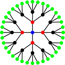
Figure 1: Structure of the a particular Cayley tree $C_{4,3}$. Nodes colored with red constitute the first shell of $C_{4,3}$; Nodes colored with black constitute the second shell of $C_{4,3}$; Nodes colored with green constitute the third shell of $C_{4,3}$.

Using the construction, one can find all nodes in the same shell are equivalent. The nodes in the outermost shell have a degree $d_{g}=1$, and all other nodes have a degree $d_{i}=m$ $(i=0,1,\cdots,g-1)$. We also find that the number of nodes of $(i=1,2,\cdots,g)$ shell $i$ is $N_{i}=m(m-1)^{i-1}$. Thus for $C_{m,g}$ the total number of nodes is

$$N=1+\sum_{i=1}^{g}N_{i}=\frac{m(m-1)^{g}-2}{m-2}\,,$$ (1)

and the total number of edges in $C_{m,g}$ is

$$E=N-1=\frac{m(m-1)^{g}-m}{m-2}\,.$$ (2)

Although Cayley trees are obviously self-similar, their fractal dimension is infinite, and they are thus nonfractal.

III Relation between Var(FRT) and $\langle$GFPT$\rangle$ on general finite networks and results of $R$(FRT) on some networks

In this section, we present and prove the general relation between the variance of FRT and the mean global first-passage time on general finite networks. Our derivations are based on the relation between their probability generating functions. To briefly review the definition probability-generating function (see e.g., Gut05 ), we designate $p_{k}$ ($k=0,1,2,\cdots$) the probability mass function of a discrete random variable $T$ that takes values of non-negative integers $\{0,1,...\}$, and we define the related probability-generating function $\Phi_{T}(z)$ of $p_{k}$,

$$\Phi_{T}(z)=\sum_{k=0}^{+\infty}z^{k}p_{k}.$$ (3)

Now we introduce the probability distribution of GFPT and FRT, and then define the probability generating functions of them. Before proceeding, we must clarify that, when evaluating the GFPT, the starting site is selected by mimicking the steady state, namely the probability that a node $u$ is selected as starting site is $d_{u}/(2E)$.

Here $P_{v\rightarrow u}(k)$ ($k=0,1,2,\cdots$) is the probability distribution of the first passage time (FPT) from node $v$ to node $u$. Thus $P_{u\rightarrow u}(k)$ ($k=0,1,2,\cdots$) is the probability distribution of FRT when the target is located at node $u$. The probability distribution of the GFPT to the target node $u$, denoted as $P_{u}(k)$ ($k=0,1,2,\cdots$), is defined

$$P_{u}(k)=\sum_{v}\frac{d_{v}}{2E}P_{v\rightarrow u}(k),$$ (4)

where the sum runs over all the nodes in the network.

We denote $\Phi_{\rm FRT}(z)$ and $\Phi_{\rm GFPT}(z)$ the probability-generating functions of the FRT and GFPT for node $u$, respectively. Both have a close connection with the probability generating function of the return time (i.e., how long it takes the walker to return to its origin, not necessarily for the first time), whose generating function is $\Phi_{\rm RT}(z)$. Note that HvKa12 ,

$$\Phi_{\rm GFPT}(z)=\frac{z}{1-z}\times\frac{d_{u}}{2E}\times\frac{1}{\Phi_{\rm RT}(z)},$$ (5)

and

$$\Phi_{\rm FRT}(z)=1-\frac{1}{\Phi_{\rm RT}(z)}.$$ (6)

Equation (5)) can now be rewritten

$$\frac{1}{\Phi_{\rm RT}(z)}=\frac{1-z}{z}\times\frac{2E}{d_{u}}\times\Phi_{\rm GFPT}(z).$$ (7)

Plugging the expression for $\frac{1}{\Phi_{\rm RT}(z)}$ into Eq. (6), we get

$$\Phi_{\rm FRT}(z)=1-\frac{1-z}{z}\times\frac{2E}{d_{u}}\times\Phi_{\rm GFPT}(z).$$ (8)

Taking the first derivative on both sides of Eq. (8) and setting $z=1$, we obtain the mean FRT,

$$\langle FRT\rangle=\left.\frac{d}{dz}\Phi_{\rm FRT}(z)\right|_{z=1}=\frac{2E}{d_{u}}.$$ (9)

Taking the second order derivative on both sides of Eq. (8) and setting $z=1$, we obtain

$$\left.\frac{d^{2}}{dz^{2}}\Phi_{\rm FRT}(z)\right|_{z=1} = \frac{2E}{d_{u}}\left\{2\left.\frac{d}{dz}\Phi_{\rm GFPT}(z)\right|_{z=1}-2\right\}$$ (10)

$$= 2\langle FRT\rangle\langle GFPT\rangle-2\langle FRT\rangle.$$

We thus get the variance

$$Var(FRT) = \left.\frac{d^{2}}{dz^{2}}\Phi_{\rm FRT}(z)\right|_{z=1}+\left.\frac{d}{dz}\Phi_{\rm FRT}(z)\right|_{z=1}-\langle FRT\rangle^{2}$$ (11)

$$= 2\langle FRT\rangle\langle GFPT\rangle-\langle FRT\rangle^{2}-\langle FRT\rangle,$$

and the reduced moment

$$R(FRT)=\frac{\sqrt{Var(FRT)}}{\langle FRT\rangle}\approx\sqrt{\frac{2\langle GFPT\rangle}{\langle FRT\rangle}-1}.$$ (12)

Both $\langle GFPT\rangle$ and $\langle FRT\rangle$ increase with the increase of network size $N$, and the order in which $\langle GFPT\rangle$ increases is no less than that of $\langle FRT\rangle$. If the order that $\langle GFPT\rangle$ increases is greater than that of $\langle FRT\rangle$, $R(FRT)\rightarrow\infty$ as $N\rightarrow\infty$. However if the order that $\langle FRT\rangle$ increases is the same as that of $\langle GFPT\rangle$, $R(FRT)\rightarrow const$ as $N\rightarrow\infty$.

If $\langle GFPT\rangle$ has been obtained on a network, $R(FRT)$ can also be obtained on that network. For example, on classical and dual Sierpinski gaskets embedded in $d$-dimensional ($d\geq 2$) Euclidian spaces, $\langle FRT\rangle\sim N$ and $\langle GFPT\rangle\sim N^{2/d_{s}}$, where $d_{s}=\frac{2ln(d+1)}{ln(d+3)}$ Weber_Klafter_10 ; Wu_Zhang_10 . Thus $R(FRT)\sim N^{\frac{ln(d+3)}{2ln(d+1)}-\frac{1}{2}}$ and

$$R(FRT)\rightarrow\infty,$$ (13)

as $N\rightarrow\infty$. We find that Eq. (13) also holds on many other networks, such as Vicsek fractals, T-graph, pseudofractal scale-free webs, ($u,v$) flowers, and fractal and non-fractal scale-free trees. Although $\langle FRT\rangle$ is easy to obtain in these networks, it is not a reliable estimate of FRT because the fluctuation of FRT is huge.

IV Fluctuation analysis of first return time on Cayley trees

We now calculate the variance, the reduced moment of FRT, and then analyze the fluctuation of FRT on Cayley trees. Note that the target location strongly affects Var(FRT) and $R(FRT)$. We calculate Var(FRT) and $R(FRT)$ when the target is located at an arbitrary node on Cayley trees. We obtain exact results for Var(FRT) and $R(FRT)$ and present their scalings with network size. The derivation presented here is based on the relation between Var(FRT) and $\langle GFPT\rangle$ expressed in Eq. (11). We first thus derive the mean GFPT Notes1 to an arbitrary node on $C_{m,g}$. We then obtain Var(FRT) and $R$(FRT) from Eqs. (11) and (12). Because the calculation is lengthy, we here summerize the the derivation and the final results and present the detailed derivation in the Appendix A–B.

IV.1 Mean GFPT and the variance of FRT while the target site is located at arbitrary node on Cayley trees

Here $\Omega$ is the node set of the Cayley tree $C_{m,g}$, and we define

$$W_{v}=\sum_{u\in\Omega}\pi(u)L_{uv},$$ (14)

and

$$\Sigma=\sum_{u\in\Omega}\pi(u)W_{u},$$ (15)

where $L_{uv}$ is the shortest path length from node $u$ to $v$, and $\pi(u)=\frac{d_{u}}{2E}$. Using the relation between the mean first passage time and the effective resistance, if the target site is fixed at node $y$ ($y\in\Omega$) we find the mean GFPT to node $y$ to be

$$\langle GFPT_{y}\rangle = E(2W_{y}-\Sigma)+1.$$ (16)

We supply the detailed derivation in Appendix A.

Note that the target location strongly affects the moments of GFPT and FRT, and that all nodes in the same shell of $C_{m,g}$ are equivalent. Here $GFPT_{i}$, $FRT_{i}$ $(i=0,1,2,\cdots,g)$ are the GFPT and FRT, respectively, and the target site is located in shell $i$ of the Cayley tree $C_{m,g}$. Note that we here regard the node in shell $0$ to be the root of the tree. Calculating $W_{v}$ for any node $v$ and $\Sigma$ and plugging their expressions into Eq. (16), we obtain the mean GFPT to the root,

$$\langle GFPT_{0}\rangle = \frac{1}{2E}\left[(m-1)^{2g}\frac{4m(m-1)}{(m-2)^{3}}\right.$$ (17)

$$-(m-1)^{g}\frac{m(4gm-3m+6)}{(m-2)^{2}}$$

$$\left.-\frac{m(3m^{2}-8m+8)}{(m-2)^{3}}\right],$$

and the mean GFPT to nodes in shell $i$ $(i=1,2,\cdots,g)$ of $C_{m,g}$,

$$\langle GFPT_{i}\rangle = (m-1)^{g}\frac{2m(m-2)i-4(m-1)}{(m-2)^{2}}$$ (18)

$$+\frac{4(m-1)^{g-i+1}}{(m-2)^{2}}+\langle GFPT_{0}\rangle.$$

We supply a detailed derivation of Eqs. (17) and (18) in Appendix B. Inserting the expressions for the mean GFPT and mean FRT into Eqs. (11), we obtain the variance of FRT for $i=0,1,2,\cdots,g-1$,

$$Var(FRT_{i}) = (m-1)^{2g}\frac{8m(m-2)i-12m+16}{(m-2)^{3}}$$ (19)

$$- (m-1)^{g}[\frac{8gm-4m+8mi}{(m-2)^{2}}+\frac{16(m-1)}{(m-2)^{3}}]$$

$$+ \frac{16(m-1)^{2g-i+1}}{(m-2)^{3}}-\frac{16(m-1)^{g-i+1}}{(m-2)^{3}}$$

$$-\frac{4m^{2}-4m}{(m-2)^{3}},$$

and for $i=g$,

$$Var(FRT_{g}) = (m-1)^{2g}\frac{8m^{2}(m-2)g-4m(m^{2}-2)}{(m-2)^{3}}$$ (20)

$$-(m-1)^{g}\frac{4m(8gm-4gm^{2}+3m^{2}-4)}{(m-2)^{3}}$$

$$-\frac{8m^{3}-8m}{(m-2)^{3}}.$$

Then the reduced moments of FRT can be exactly determined using Eq. (12).

IV.2 Scalings

Using the results found in the previous subsections we derive their scalings with network size $N$. Note that $N=\frac{m(m-1)^{g}-2}{m-2}\sim(m-1)^{g}$(see Sec. II). We get $g\sim ln(N)$, $E=N-1\sim N$, and $\langle FRT_{i}\rangle\sim N$ for any $i$. We further reshuffle Eqs. (17), (18), (19), and (20) and get for $i=0,1,\cdots,g$

$$\langle GFPT_{i}\rangle\sim(i+1)N,$$ (21)

and

$$Var(FRT_{i})\sim(i+1)N^{2}.$$ (22)

If we now set $i=g$ in Eqs. (21) and (22) we obtain

$$\langle GFPT_{g}\rangle\sim Nln(N),$$ (23)

and

$$Var(FRT_{g})\sim N^{2}ln(N).$$ (24)

Inserting the expressions for $Var(FRT_{i})$ and $\langle FRT_{i}\rangle$ into Eq. (12), we obtain the reduced moment of FRT and find that in the large size limit (i.e., when $N\rightarrow\infty$), for $i=0,1,\cdots,g-1$,

$$R(FRT_{i})\rightarrow\sqrt{2mi-\frac{3m-4}{m-2}+\frac{4(m-1)^{1-i}}{m-2}},$$ (25)

and

$$R(FRT_{g})\approx\sqrt{4g-\frac{m^{2}+2m-4}{m(m-2)}}\rightarrow\infty.$$ (26)

Results show that in the large size limit, $R(FRT_{i})$ increases as $i$ increases, which implies that the farther the distance between target and root, the greater the fluctuation of FRT. If the target site is fixed at the root (i.e. $i=0$), $R(FRT_{i})$ reach its minimum

$$R(FRT_{0})\rightarrow\sqrt{\frac{m}{m-2}}.$$ (27)

If the target site is fixed at shell $i$ (i.e., $i$ does not increase as $N$ increases), $R(FRT_{i})\rightarrow const$. Here the fluctuation of FRT is small and $\langle FRT\rangle$ can be used to estimate FRT. If $i$ increases with the network size $N$, e.g., the target is located at the outermost shell (i.e. $i=g\sim ln(N)$), $i\rightarrow\infty$ as $N\rightarrow\infty$. Thus $R(FRT_{i})\rightarrow\infty$. Here the fluctuation of FRT is huge and $\langle FRT\rangle$ is not a reliable estimate of FRT.

V Conclusions

We have found the exact relation between Var(FRT) and $\langle GFPT\rangle$ in a general finite network. We thus can determine the exact variance Var(FRT) and reduced moment $R(FRT)$ because $\langle GFPT\rangle$ has been widely studied and measured on many different networks. We use the reduced moment to measure and evaluate the fluctuation of a random variable and to determine whether the mean of a random variable is a good estimate of the random variable. The greater the reduced moment, the worse the estimate provided by the mean.

In our research we find that in the large size limit (i.e., when $N\rightarrow\infty$), $R(FRT)\rightarrow\infty$, which indicates that FRT has a huge fluctuation and that $\langle FRT\rangle$ is not a reliable estimate of FRT in most networks we studied. However for random walks on Cayley trees, in most cases, $R(FRT)\rightarrow const$.

We also find that target location strongly affects FRT fluctuation on Cayley trees. Results show that the farther the distance between target and root, the greater the FRT fluctuations. $R(FRT)$ reaches its minimum when the target is located at the root of the tree, and $R(FRT)$ reaches its maximum when the target is located at the outermost shell of the tree. Results also show that when the target site is fixed at shell $i$ (i.e., $i$ does not increase as $N$ increases), $R(FRT_{i})\rightarrow const$. Here the fluctuation of FRT is small and $\langle FRT\rangle$ can be used to estimate FRT. When $i$ increases with network size $N$ (e.g., i=g), $R(FRT_{i})\rightarrow\infty$. Here the fluctuation of FRT is huge and $\langle FRT\rangle$ is not a reliable estimate of FRT.

Appendix A Derivation of Eq. 16

We denote $\Omega$ the node set of any graph $G$. For any two nodes $x$ and $y$ of graph $G$, $F(x,y)$ is the mean FPT from $x$ to $y$. Therefore $F(y,y)$ is just the first return time for node $y$. For any different two nodes $x$ and $y$, the sum

$$k(x,y)=F(x,y)+F(y,x)$$

is the commute time, and the mean FPT can be expressed in terms of commute times Te91

$$F(x,y)=\frac{1}{2}\left(k(x,y)+\sum_{u\in\Omega}\pi(u)[k(y,u)-k(x,u)]\right),$$ (28)

where $\pi(u)=\frac{d_{u}}{2E}$ is the stationary distribution for random walks on the $G$, $E$ is the total numbers of edges of graph $G$, and $d_{u}$ is the degree of node $u$.

We treat these systems as electrical networks, consider each edge a unit resistor, and denote $\mathfrak{R}_{xy}$ the effective resistance between nodes $x$ and $y$. Prior research Te91 indicates that

$$k(x,y)=2E\mathfrak{R}_{xy}.$$ (29)

If graph $G$ is a tree, the effective resistance between any two nodes is the shortest path length between the two nodes. Hence

$$\mathfrak{R}_{xy}=L_{xy},$$ (30)

where $L_{xy}$ is the shortest path length between node $x$ to node $y$. Thus

$$k(x,y)=2EL_{xy}.$$ (31)

Substituting $k(x,y)$ in the right side of Eq. (31), in Eq. (28) the mean FPT from $x$ to $y$ can be rewritten

$$F(x,y) = E(L_{xy}+W_{y}-W_{x}).$$ (32)

Thus the mean GFPT to $y$ can be written

$$\langle GFPT_{y}\rangle = \sum_{x\in\Omega}\pi(x)F(x,y)$$ (33)

$$= \pi(y)F(y,y)+\sum_{x\neq y}\pi(x)F(x,y)$$

$$= 1+\sum_{x\neq y}\pi(x)E(L_{xy}+W_{y}-W_{x})$$

$$= 1+E\sum_{x\neq y}\pi(x)L_{xy}+E\sum_{x\neq y}\pi(x)W_{y}$$

$$-E\sum_{x\neq y}\pi(x)W_{x})$$

$$= 1+EW_{y}+E(1-\pi(y))W_{y}$$

$$-E\sum_{x\neq y}\pi(x)W_{x})$$

$$= E(2W_{y}-\Sigma)+1.$$

Appendix B Derivation of Eqs. (17) and (18)

We here derive $\langle GFPT_{i}\rangle$ for any $(i=0,1,2,\cdots,g)$. To calculate $\langle GFPT_{i}\rangle$, we assume the target is located at node $v_{i}$ in shell $i$ of $C_{m,g}$. Thus $\langle GFPT_{i}\rangle$ can also be denoted $\langle GFPT_{v_{i}}\rangle$. Using Eq. (16), we calculate $W_{v_{i}}$ and $\Sigma$ defined in Eqs. (14) and (15).

Calculating the shortest path length between any two nodes in a Cayley tree is straightforward, e.g., the shortest path length between arbitrary node $u$ in shell $i$ is $(i=1,2,\cdots,g)$ and the root $v_{0}$ is $L_{uv_{0}}=i$. Thus for root node $v_{0}$,

$$W_{v_{0}} \equiv \sum_{u\in\Omega}\pi(u)L_{uv_{0}}$$ (34)

$$= \frac{1}{2E}\left\{\sum_{i=1}^{g-1}[m^{2}i(m-1)^{i-1}]+mg(m-1)^{g-1}\right\}$$

$$= \frac{m(m-1)^{g}(2gm-4g-m)+m^{2}}{2E\times(m-2)^{2}}.$$

For arbitrary node $v_{i}$ in shell $i$ ($i=1,2,\cdots,g$), we can find its parents node in shell $i-1$ and let $v_{i-1}$ denotes the parents node of $v_{i}$ and $\Omega_{i}$ denotes the nodes set of the subtree whose root is $v_{i}$. We find that

$$L_{uv_{i}}-L_{uv_{i-1}}=\left\{\begin{array}[]{ll}-1&u\in\Omega_{i}\\ 1&\textrm{otherwise}\end{array}\right..$$

Hence,

$$W_{v_{i}}-W_{v_{i-1}}$$

$$= \sum_{u\in\Omega}\pi(u)(L_{uv_{i}}-L_{uv_{i-1}})$$

$$= \sum_{u\in\Omega}\pi(u)-2\sum_{u\in\Omega_{i}}\pi(u)$$

$$= 1-\frac{1}{E}\left\{\sum_{k=i}^{g-1}m(m-1)^{k-i}+(m-1)^{g-i}\right\}$$

$$= 1-\frac{1}{E}\left\{\frac{2}{m-2}(m-1)^{g-i+1}-\frac{m}{m-2}\right\}.$$

Thus,

$$W_{v_{i}}-W_{v_{0}}$$ (35)

$$= \sum_{k=1}^{i}(W_{v_{k}}-W_{v_{k-1}})$$

$$= i-\frac{1}{E}\left\{\sum_{k=1}^{i}\frac{2}{m-2}(m-1)^{g-k+1}-\frac{mi}{m-2}\right\}.$$

$$= i-\frac{2(m-1)^{g+1}-2(m-1)^{g-i+1}-mi(m-2)}{(m-2)^{2}E}$$

$$= \frac{mi(m-2)(m-1)^{g}-2(m-1)^{g+1}}{E\times(m-2)^{2}}$$

$$+ \frac{2(m-1)^{g-i+1}}{E\times(m-2)^{2}}.$$

Therefore, for any $i=1,2,\cdots,g$,

$$\langle GFPT_{i}\rangle-\langle GFPT_{0}\rangle=2E(W_{v_{i}}-W_{v_{0}})$$ (36)

$$= (m-1)^{g}\frac{2m(m-2)i-4(m-1)}{(m-2)^{2}}$$

$$+\frac{4(m-1)^{g-i+1}}{(m-2)^{2}},$$

and Eq. (18) is obtained.

Replacing $W_{v_{0}}$ from Eq. (34) in Eq. (35), we obtain

$$W_{v_{i}} = \frac{(2gm^{2}-4gm-4im-4m+2im^{2}-m^{2}+4)(m-1)^{g}}{2E\times(m-2)^{2}}$$ (37)

$$+ \frac{4(m-1)^{g-i+1}+m^{2}}{2E\times(m-2)^{2}}.$$

Hence,

$$\Sigma = \sum_{u\in\Omega}\pi(u)W_{u}$$ (38)

$$= \frac{mW_{v_{0}}+\sum_{i=1}^{g-1}m^{2}(m-1)^{i-1}W_{v_{i}}+m(m-1)^{g-1}W_{v_{g}}}{2E}$$

$$= \frac{2m(2gm^{2}-2m-4gm-m^{2}+2)(m-1)^{2g}}{2(m-2)^{3}2E^{2}}$$

$$+ \frac{m(3m^{2}+4m-4)(m-1)^{g}-m^{3}}{2(m-2)^{3}2E^{2}}.$$

Therefore,

$$\langle GFPT_{0}\rangle = E(2W_{v_{0}}-\Sigma)+1$$ (39)

$$= \frac{1}{2E}\left[(m-1)^{2g}\frac{4m(m-1)}{(m-2)^{3}}\right.$$

$$-(m-1)^{g}\frac{m(4gm-3m+6)}{(m-2)^{2}}$$

$$\left.-\frac{m(3m^{2}-8m+8)}{(m-2)^{3}}\right],$$

and Eq. (17) is obtained.

References

- (1) S. Redner, A Guide to First-Passage Processes (Cambridge University Press, Cambridge, UK, 2007).
- (2) Eds. R. Metzler, G. Oshanin, S. Redner, First-Passage Phenomena and Their Applications, (World Scientific Publishing, Singapore, 2014).
- (3) A. Bunde, J. Kropp, and H.-J. Schellnhuber, The Science of Disasters, (Springer, Berlin, 2005).
- (4) M. R. Leadbetter, G. Lindgren, and H. Rootz n, Extremes and Related Properties of Random Sequences and Processes, (Springer-Verlag, New York, Heidelberg, Berlin, 1983).
- (5) R. D. Reiss, M. Thomas, and R. D. Reiss, Statistical Analysis of Extreme Values: From Insurance, Finance, Hydrology and Other Fields, (Birkhauser, Boston, 1997).
- (6) K. Y. Kondratyev, C. A. Varotsos, and V. F. Krapivin, Natural Disasters as Interactive Components of Global Ecodynamics, (Springer, Berlin, 2006).
- (7) J. A. Battjes and H. Gerritsen, Philos. Trans. R. Soc. London, Ser. A 360, 1461 (2002).
- (8) V. Kishore, M. S. Santhanam, and R. E.Amritkar, Phys. Rev. Lett. 106, 188701 (2011).
- (9) Y. Z. Chen, Z. G. Huang and Y. Cheng. Lai, Sci. Rep. 18(4), 6121 (2014).
- (10) J. F. Eichner, J. W. Kantelhardt, A. Bunde and S. Havlin, Phys. Rev. E 75, 011128 (2007).
- (11) C Nicolis S. C. Nicolis, Europhys. Lett., 80,40003 (2007).
- (12) N. R. Moloney and J. Davidsen, Phys. Rev. E 79, 041131 (2009)
- (13) C. Liu, Z. Q. Jiang, F. Ren and W. X. Zhou, Phys. Rev. E 80, 046304 (2009).
- (14) N. Hadyn, J. Luevano, G. Mantica, S. Vaienti Phys. Rev. Lett. 88, 224502 (2002).
- (15) O. C. Martin and P. Sulc, Phys. Rev. E 81, (2010)031111.
- (16) N. Masuda and N. Konno, Phys. Rev. E 69, (2004)066113.
- (17) C.P. Lowea and A.J. Masters, Physica A 286 10 (2000).
- (18) M. S. Santhanam and H. Kantz, Phys. Rev. E 78, 051113 (2008)
- (19) L. Palatella and C. Pennetta, Phys. Rev. E 83, 041102 (2011).
- (20) A. Bunde, J. F. Eichner, S. Havlin, and J. W. Kantelhardt, Physica A 330, 1 (2003).
- (21) A. Bunde, J. F. Eichner, J. W. Kantelhardt, and S. Havlin, Phys. Rev. Lett. 94, 048701 (2005).
- (22) P. Olla, Phys. Rev. E 76, 011122 (2007).
- (23) P. Chelminiak, Physics Letters A 375 3114(2011)
- (24) F.M. Izrailev, A. Castaneda-Mendoza, Physics Letters A 350 355(2006)
- (25) C.P. Haynes, A.P. Roberts, Phys. Rev. E 78, 041111 (2008).
- (26) L. Lovász, Combinatorics: Paul erdös is eighty (Keszthely, Hungary, 1993), vol. 2, issue 1, p. 1-46.
- (27) V.Tejedor O. Bénichou, R. Voituriez, Phys Rev E 80, 065104(R) (2009).
- (28) O. Chepizhko and F. Peruani, Phys. Rev. Lett. 111, 160604 (2013).
- (29) B. Meyer, C. Chevalier, R. Voituriez, and O. Bénichou, Phys. Rev. E 83, 051116 (2011).
- (30) S. Condamin, O. Bénichou, V. Tejedor, R. Voituriez and J. Klafter, Nature 450, 77 (2007).
- (31) O. Bénichou, R. Voituriez, Phys. Rep. 539, 225 (2014).
- (32) A. Kittas, S. Carmi, S. Havlin and P. Argyrakis, Europhys. Lett. 84, 40008, (2008).
- (33) Z. Y. Chen and C. Cai, Macromolecules 32, 5423 (1999).
- (34) O. Mülken, V. Bierbaum, and A. Blumen, J. Chem. Phys. 124, 124905 (2006).
- (35) F. Fürstenberg, M. Dolgushev, and A. Blumen, J. Chem. Phys. 136, 154904 (2012)
- (36) A. Bar-Haim, J. Klafter, and R. Kopelman, J. Am. Chem. Soc. 119, 6197 (1997).
- (37) A. Bar-Haim and J. Klafter, J. Phys. Chem. B 102, 1662 (1998).
- (38) J. L. Bentz, F. N. Hosseini, and J. J. Kozak, Chem. Phys. Lett. 370, 319 (2003).
- (39) J. L. Bentz and J. J. Kozak, J. Lumin. 121, 62 (2006).
- (40) I. M. Sokolov, J. Mai, and A. Blumen, Phys. Rev. Lett. 79, 857 (1997).
- (41) A. Blumen and G. Zumofen, J. Chem. Phys. 75, 892 (1981).
- (42) B. Wu, Y. Lin, Z. Z. Zhang, and G. R. Chen, J. Chem. Phys. 137, 044903 (2012).
- (43) Y. Lin and Z. Z. Zhang, J. Chem. Phys. 138, 094905 (2013).
- (44) J. L. Bentz, J. W. Turner, J. J. Kozak Phys. Rev. E 82, 011137 (2010).
- (45) S. Weber, J. Klafter, A. Blumen, Phys. Rev. E 82, 051129 (2010).
- (46) S.Q. Wu, Z. Z. Zhang and G. R. Chen, Eur. Phys. J. B 82, 91 (2011).
- (47) A. Blumen, C. V. Ferber, A. Jurjiu and T. Koslowski, Macromolecules 37, 638 (2004).
- (48) J. H. Peng, J. Stat. Mech.: Theor. Exp. P12018 (2014).
- (49) E. Agliari, Phys. Rev. E 77, 011128 (2008).
- (50) Z. Z. Zhang, Y. Lin, S. G. Zhou, B. Wu, and J. H. Guan, New J. Phys. 11, 103043 (2009).
- (51) J. H. Peng and G. Xu, J. Chem. Phys. 40, 134102 (2014).
- (52) Z. Z. Zhang, Y. Qi, S. G. Zhou, W. L. Xie and J. H. Guan, Phys. Rev. E 79, 021127 (2009).
- (53) J. H. Peng, E. Agliari, Z.Z. Zhang, Chaos 25, 073118 (2015).
- (54) Z. Z. Zhang, W. L. Xie, S. G. Zhou, S. Y. Gao, J. H. Guan, Europhys. Lett. 88, 10001 (2009).
- (55) S. Hwang, C.K. Yun, D.S. Lee, B. Kahng, D. Kim, Phys. Rev. E 82, 056110 (2010).
- (56) B. Meyer, E. Agliari, O. Bénichou, and R. Voituriez, Phys. Rev. E 85, 026113 (2012).
- (57) J. H. Peng and E. Agliari, Chaos, 27, 083108 (2017).
- (58) Z. Z. Zhang , Y. Lin and Y. J. Ma, J. Phys. A: Math. Theor. 44, 075102 (2011).
- (59) J. H. Peng and G. Xu, J. Stat. Mech.: Theor. Exp. P04032 (2014).
- (60) J. H. Peng, J. Xiong and G. Xu, Physica A 407, 231 (2014).
- (61) F. Comellas, A. Miralles, Phys. Rev. E 81, 061103 (2010).
- (62) Y. Lin, B. Wu, and Z. Z. Zhang, Phys. Rev. E 82, 031140 (2010).
- (63) M. Ostilli, Physica A 391, 3417 (2012).
- (64) A. Gut, Probability: A Graduate Course (Springer, New York, 2005).
- (65) S. Hwang, D.-S. Lee, B. Kahng, Phys. Rev. Lett. 109, 088701 (2012).
- (66) Note: In general there are two definitions for the GFPT due to different ways that the starting site is selected. In the first, all nodes of the network have an equal probability of being selected as the starting site. In the second, the starting site is selected by mimicking the steady state, i.e., the probability that a node is selected as starting site is . In this paper, we have adopted the second definition of the GFPT. On the Cayley trees, the mean GFPT using the first definition is obtained, but the mean GFPT using the second definition remains unknown.
- (67) P. Tetali, J. Theoretical Probability, 4, 101 (1991).