Zeroth-Order Stochastic Variance Reduction for Nonconvex Optimization

Abstract

As application demands for zeroth-order (gradient-free) optimization accelerate, the need for variance reduced and faster converging approaches is also intensifying. This paper addresses these challenges by presenting: a) a comprehensive theoretical analysis of variance reduced zeroth-order (ZO) optimization, b) a novel variance reduced ZO algorithm, called ZO-SVRG, and c) an experimental evaluation of our approach in the context of two compelling applications, black-box chemical material classification and generation of adversarial examples from black-box deep neural network models. Our theoretical analysis uncovers an essential difficulty in the analysis of ZO-SVRG: the unbiased assumption on gradient estimates no longer holds. We prove that compared to its first-order counterpart, ZO-SVRG with a two-point random gradient estimator could suffer an additional error of order $O(1/b)$, where $b$ is the mini-batch size. To mitigate this error, we propose two accelerated versions of ZO-SVRG utilizing variance reduced gradient estimators, which achieve the best rate known for ZO stochastic optimization (in terms of iterations). Our extensive experimental results show that our approaches outperform other state-of-the-art ZO algorithms, and strike a balance between the convergence rate and the function query complexity.

1 Introduction

Zeroth-order (gradient-free) optimization is increasingly embraced for solving machine learning problems where explicit expressions of the gradients are difficult or infeasible to obtain. Recent examples have shown zeroth-order (ZO) based generation of prediction-evasive, black-box adversarial attacks on deep neural networks (DNNs) as effective as state-of-the-art white-box attacks, despite leveraging only the inputs and outputs of the targeted DNN [1, 2, 3]. Additional classes of applications include network control and management with time-varying constraints and limited computation capacity [4, 5], and parameter inference of black-box systems [6, 7]. ZO algorithms achieve gradient-free optimization by approximating the full gradient via gradient estimators based on only the function values [8, 9].

Although many ZO algorithms have recently been developed and analyzed [5, 10, 11, 12, 13, 14, 15, 16, 17, 18], they often suffer from the high variances of ZO gradient estimates, and in turn, hampered convergence rates. In addition, these algorithms are mainly designed for convex settings, which limits their applicability in a wide range of (non-convex) machine learning problems.

In this paper, we study the problem of design and analysis of variance reduced and faster converging nonconvex ZO optimization methods. To reduce the variance of ZO gradient estimates, one can draw motivations from similar ideas in the first-order regime. The stochastic variance reduced gradient (SVRG) is a commonly-used, effective first-order approach to reduce the variance [19, 20, 21, 22, 23]. Due to the variance reduction, it improves the convergence rate of stochastic gradient descent (SGD) from $O({1}/{\sqrt{T}})$ to $O({1}/{{T}})$, where $T$ is the total number of iterations.

Although SVRG has shown a great promise, applying similar ideas to ZO optimization is not a trivial task. The main challenge arises due to the fact that SVRG relies upon the assumption that a stochastic gradient is an unbiased estimate of the true batch/full gradient, which unfortunately does not hold in the ZO case. Therefore, it is an open question whether the ZO stochastic variance reduced gradient could enable faster convergence of ZO algorithms. In this paper, we attempt to fill the gap between ZO optimization and SVRG.

Contributions We propose and evaluate a novel ZO algorithm for nonconvex stochastic optimization, ZO-SVRG, which integrates SVRG with ZO gradient estimators. We show that compared to SVRG, ZO-SVRG achieves a similar convergence rate that decays linearly with $O(1/T)$ but up to an additional error correction term of order $1/b$, where $b$ is the mini-batch size. Without a careful treatment, this correction term (e.g., when $b$ is small) could be a critical factor affecting the optimization performance. To mitigate this error term, we propose two accelerated ZO-SVRG variants, utilizing reduced variance gradient estimators. These yield a faster convergence rate towards $O(d/T)$, the best known iteration complexity bound for ZO stochastic optimization.

Our work offers a comprehensive study on how ZO gradient estimators affect SVRG on both iteration complexity (i.e., convergence rate) and function query complexity. Compared to the existing ZO algorithms, our methods can strike a balance between iteration complexity and function query complexity. To demonstrate the flexibility of our approach in managing this trade-off, we conduct an empirical evaluation of our proposed algorithms and other state-of-the-art algorithms on two diverse applications: black-box chemical material classification and generation of universal adversarial perturbations from black-box deep neural network models. Extensive experimental results and theoretical analysis validate the effectiveness of our approaches.

2 Related work

In ZO algorithms, a full gradient is typically approximated using either a one-point or a two-point gradient estimator, where the former acquires a gradient estimate $\hat{\nabla}f(\mathbf{x})$ by querying $f(\cdot)$ at a single random location close to $\mathbf{x}$ [10, 11], and the latter computes a finite difference using two random function queries [12, 13]. In this paper, we focus on the two-point gradient estimator since it has a lower variance and thus improves the complexity bounds of ZO algorithms.

Despite the meteoric rise of two-point based ZO algorithms, most of the work is restricted to convex problems [5, 14, 15, 16, 17, 18]. For example, a ZO mirror descent algorithm proposed by [14] has an exact rate $O({\sqrt{d}}/{\sqrt{T}})$, where $d$ is the number of optimization variables. The same rate is obtained by bandit convex optimization [15] and ZO online alternating direction method of multipliers [5]. Current studies suggested that ZO algorithms typically agree with the iteration complexity of first-order algorithms up to a small-degree polynomial of the problem size $d$.

In contrast to the convex setting, non-convex ZO algorithms are comparatively under-studied except a few recent attempts [7, 13, 24, 25, 26]. Different from convex optimization, the stationary condition is used to measure the convergence of nonconvex methods. In [13], the ZO gradient descent (ZO-GD) algorithm was proposed for deterministic nonconvex programming, which yields $O({d}/{T})$ convergence rate. A stochastic version of ZO-GD (namely, ZO-SGD) studied in [24] achieves the rate of $O({\sqrt{d}}/{\sqrt{T}})$. In [25], a ZO distributed algorithm was developed for multi-agent optimization, leading to $O({1}/{T}+{d}/{q})$ convergence rate. Here $q$ is the number of random directions used to construct a gradient estimate. In [7], an asynchronous ZO stochastic coordinate descent (ZO-SCD) was derived for parallel optimization and achieved the rate of $O({\sqrt{d}}/{\sqrt{T}})$. In [26], a variant of ZO-SCD, known as ZO stochastic variance reduced coordinate (ZO-SVRC) descent, improved the convergence rate from $O({\sqrt{d}}/{\sqrt{T}})$ to $O({{d}}/{{T}})$ under the same parameter setting for the gradient estimation. Although the authors in [26] considered the stochastic variance reduced technique, only a coordinate descent algorithm using a coordinate-wise (deterministic) gradient estimator was studied. This motivates our study on a more general framework ZO-SVRG under different gradient estimators.

3 Preliminaries

Consider a nonconvex finite-sum problem of the form

$$\begin{array}[]{ll}\displaystyle\operatorname*{\text{minimize}}_{\mathbf{x}\in\mathbb{R}^{d}}&\displaystyle f(\mathbf{x})\mathrel{\mathop{:}}=\frac{1}{n}\sum_{i=1}^{n}f_{i}(\mathbf{x}),\end{array}$$ (1)

where $\{f_{i}(\mathbf{x})\}_{i=1}^{n}$ are $n$ individual nonconvex cost functions. The generic form (1) encompasses many machine learning problems, ranging from generalized linear models to neural networks. We next elaborate on assumptions of problem (1), and provide a background on ZO gradient estimators.

3.1 Assumptions

A1: Functions $\{f_{i}\}$ have $L$-Lipschitz continuous gradients ($L$-smooth), i.e., $\|\nabla f_{i}(\mathbf{x})-\nabla f_{i}(\mathbf{y})\|_{2}\leq L\|\mathbf{x}-\mathbf{y}\|_{2}$ for any $\mathbf{x}$ and $\mathbf{y}$, $i\in[n]$, and some $L<\infty$. Here $\|\cdot\|_{2}$ denotes the Euclidean norm, and for ease of notation $[n]$ represents the integer set $\{1,2,\ldots,n\}$.

A2: The variance of stochastic gradients is bounded as $\frac{1}{n}\sum_{i=1}^{n}\|\nabla f_{i}(\mathbf{x})-\nabla f(\mathbf{x})\|_{2}^{2}\leq\sigma^{2}$. Here $\nabla f_{i}(\mathbf{x})$ can be viewed as a stochastic gradient of $\nabla f(\mathbf{x})$ by randomly picking an index $i\in[n]$.

Both A1 and A2 are the standard assumptions used in nonconvex optimization literature [7, 13, 23, 24, 25, 26]. Note that A2 is milder than the assumption of bounded gradients [5, 25]. For example, if $\|\nabla f_{i}(\mathbf{x})\|_{2}\leq\tilde{\sigma}$, then A2 is satisfied with $\sigma=2\tilde{\sigma}$.

3.2 ZO gradient estimation

Given an individual cost function $f_{i}$ (or an arbitrary function under A1 and A2), a two-point random gradient estimator $\hat{\nabla}f_{i}(\mathbf{x})$ is defined by [13, 16]

$$\hat{\nabla}f_{i}(\mathbf{x})=(d/\mu)\left[f_{i}(\mathbf{x}+\mu\mathbf{u}_{i})-f_{i}(\mathbf{x})\right]\mathbf{u}_{i},~{}\text{for}~{}i\in[n],$$ (RandGradEst)

where recall that $d$ is the number of optimization variables, $\mu>0$ is a smoothing parameter, and $\{\mathbf{u}_{i}\}$ are i.i.d. random directions drawn from a uniform distribution over a unit sphere [10, 15, 16]. In general, RandGradEst is a biased approximation to the true gradient ${\nabla}f_{i}(\mathbf{x})$, and its bias reduces as $\mu$ approaches zero. However, in a practical system, if $\mu$ is too small, then the function difference could be dominated by the system noise and fails to represent the function differential [7].

Remark 1

Instead of using a single sample $\mathbf{u}_{i}$ in RandGradEst, the average of $q$ i.i.d. samples $\{\mathbf{u}_{i,j}\}_{j=1}^{q}$ can also be used for gradient estimation [5, 14, 25],

$$\textstyle\hat{\nabla}f_{i}(\mathbf{x})=(d/(\mu q))\sum_{j=1}^{q}\left[f_{i}(\mathbf{x}+\mu\mathbf{u}_{i,j})-f_{i}(\mathbf{x})\right]\mathbf{u}_{i,j},~{}\text{for}~{}i\in[n],$$ (Avg-RandGradEst)

which we call an average random gradient estimator.

In addition to RandGradEst and Avg-RandGradEst, the work [7, 26, 27] considered a coordinate-wise gradient estimator. Here every partial derivative is estimated via the two-point querying scheme under fixed direction vectors,

$$\textstyle\hat{\nabla}f_{i}(\mathbf{x})=\sum_{\ell=1}^{d}\left(1/(2\mu_{\ell})\right)\left[f_{i}(\mathbf{x}+\mu_{\ell}\mathbf{e}_{\ell})-f_{i}(\mathbf{x}-\mu_{\ell}\mathbf{e}_{\ell})\right]\mathbf{e}_{l},~{}\text{for}~{}i\in[n],$$ (CoordGradEst)

where $\mu_{\ell}>0$ is a coordinate-wise smoothing parameter, and $\mathbf{e}_{\ell}\in\mathbb{R}^{d}$ is a standard basis vector with $1$ at its $\ell$th coordinate, and $0$s elsewhere. Compared to RandGradEst, CoordGradEst is deterministic and requires $d$ times more function queries. However, as will be evident later, it yields an improved iteration complexity (i.e., convergence rate). More details on ZO gradient estimation can be found in Appendix A.1.

4 ZO stochastic variance reduced gradient (ZO-SVRG)

4.1 SVRG: from first-order to zeroth-order

It has been shown in [19, 20] that the first-order SVRG achieves the convergence rate $O({1}/{T})$, yielding $O(\sqrt{T})$ less iterations than the ordinary SGD for solving finite sum problems. The key step of SVRG (Algorithm 1) is to generate an auxiliary sequence $\hat{\mathbf{x}}$ at which the full gradient is used as a reference in building a modified stochastic gradient estimate

$$\textstyle\hat{\mathbf{g}}=\nabla f_{\mathcal{I}}(\mathbf{x})-(\nabla f_{\mathcal{I}}(\hat{\mathbf{x}})-\nabla f(\hat{\mathbf{x}})),~{}\nabla f_{\mathcal{I}}(\mathbf{x})=(1/b)\sum_{i\in{\mathcal{I}}}{\nabla}f_{i}({\mathbf{x}})$$ (2)

where $\hat{\mathbf{g}}$ denotes the gradient estimate at $\mathbf{x}$, $\mathcal{I}\subseteq[n]$ is a mini-batch of size $b$ (chosen uniformly randomly), and $\nabla f(\mathbf{x})=\nabla f_{[n]}(\mathbf{x})$. The key property of (2) is that $\hat{\mathbf{g}}$ is an unbiased gradient estimate of $\nabla f(\mathbf{x})$. The gradient blending (2) is also motivated by a variance reduced technique known as control variate [28, 29, 30]. The link between SVRG and control variate is discussed in Appendix A.2.

In the ZO setting, the gradient blending (2) is approximated using only function values,

$$\textstyle\hat{\mathbf{g}}=\hat{\nabla}f_{\mathcal{I}}(\mathbf{x})-(\hat{\nabla}f_{\mathcal{I}}(\hat{\mathbf{x}})-\hat{\nabla}f(\hat{\mathbf{x}})),~{}\hat{\nabla}f_{\mathcal{I}}(\mathbf{x})=(1/b)\sum_{i\in{\mathcal{I}}}\hat{\nabla}f_{i}({\mathbf{x}}),$$ (3)

where $\hat{\nabla}f(\mathbf{x})=\hat{\nabla}f_{[n]}(\mathbf{x})$, and $\hat{\nabla}f_{i}$ is a ZO gradient estimate specified by RandGradEst, Avg-RandGradEst or CoordGradEst. Replacing (2) with (3) in SVRG (Algorithm 1) leads to a new ZO algorithm, which we call ZO-SVRG (Algorithm 2). We highlight that although ZO-SVRG is similar to SVRG except the use of ZO gradient estimators to estimate batch, mini-batch, as well as blended gradients, this seemingly minor difference yields an essential difficulty in the analysis of ZO-SVRG. That is, the unbiased assumption on gradient estimates used in SVRG no longer holds. Thus, a careful analysis of ZO-SVRG is much needed.

4.2 ZO-SVRG and convergence analysis

In what follows, we focus on the analysis of ZO-SVRG using RandGradEst. Later, we will study ZO-SVRG with Avg-RandGradEst and CoordGradEst. We start by investigating the second-order moment of the blended ZO gradient estimate $\hat{\mathbf{v}}_{k}^{s}$ in the form of (3); see Proposition 1.

Algorithm 1: $\text{SVRG}(T,m,\{\eta_{k}\},b,\tilde{\mathbf{x}}_{0})$

1:Input: total number of iterations $T$, epoch length $m$, number of epochs $S=\lceil T/m\rceil$, step sizes $\{\eta_{k}\}_{k=0}^{m-1}$, mini-batch $b$, and $\tilde{\mathbf{x}}_{0}$.

2:for $s=1,2,\ldots,S$ do

3:     set ${\mathbf{g}}_{s}=\nabla f(\tilde{\mathbf{x}}_{s-1})$, $\mathbf{x}_{0}^{s}=\tilde{\mathbf{x}}_{s-1}$,

4:     for $k=0,1,\ldots,m-1$ do

5:         choose mini-batch ${\mathcal{I}}_{k}$ of size $b$,

6:         compute gradient blending via (2):           $\mathbf{v}_{k}^{s}={\nabla}f_{\mathcal{I}_{k}}({\mathbf{x}}_{k}^{s})-{\nabla}f_{\mathcal{I}_{k}}({\mathbf{x}}_{0}^{s})+{\mathbf{g}}_{s}$,

7:         update $\mathbf{x}_{k+1}^{s}=\mathbf{x}_{k}^{s}-\eta_{k}\mathbf{v}_{k}^{s}$,

8:     end for

9:     set $\tilde{\mathbf{x}}_{s}=\mathbf{x}_{m}^{s}$,

10:end for

11:return $\bar{\mathbf{x}}$ chosen uniformly random from $\{\{{\mathbf{x}}_{k}^{s}\}_{k=0}^{m-1}\}_{s=1}^{S}$.

Algorithm 2: $\text{ZO-SVRG}(T,m,\{\eta_{k}\},b,\tilde{\mathbf{x}}_{0},\mu)$

1:Input: In addition to parameters in SVRG, set smoothing parameter $\mu>0$.

2:for $s=1,2,\ldots,S$ do

3:     compute ZO estimate $\hat{\mathbf{g}}_{s}=\hat{\nabla}f(\tilde{\mathbf{x}}_{s-1})$,

4:     set $\mathbf{x}_{0}^{s}=\tilde{\mathbf{x}}_{s-1}$,

5:     for $k=0,1,\ldots,m-1$ do

6:         choose mini-batch ${\mathcal{I}}_{k}$ of size $b$,

7:         compute ZO gradient blending (3):           $\hat{\mathbf{v}}_{k}^{s}=\hat{\nabla}f_{{\mathcal{I}}_{k}}({\mathbf{x}}_{k}^{s})-\hat{\nabla}f_{{\mathcal{I}}_{k}}({\mathbf{x}}_{0}^{s})+\hat{\mathbf{g}}_{s}$,

8:         update $\mathbf{x}_{k+1}^{s}=\mathbf{x}_{k}^{s}-\eta_{k}\hat{\mathbf{v}}_{k}^{s}$,

9:     end for

10:     set $\tilde{\mathbf{x}}_{s}=\mathbf{x}_{m}^{s}$,

11:end for

12:return $\bar{\mathbf{x}}$ chosen uniformly random from $\{\{{\mathbf{x}}_{k}^{s}\}_{k=0}^{m-1}\}_{s=1}^{S}$.

Proposition 1

Suppose A2 holds and RandGradEst is used in Algorithm 2. The blended ZO gradient estimate $\hat{\mathbf{v}}_{k}^{s}$ in Step 7 of Algorithm 2 satisfies

$$\mathbb{E}[\|\hat{\mathbf{v}}_{k}^{s}\|_{2}^{2}]\leq\frac{4(b+18{\color[rgb]{0,0,0}\delta_{n}})d}{b}\mathbb{E}\left[\|\nabla f(\mathbf{x}_{k}^{s})\|_{2}^{2}\right]+\frac{6(4d+1)L^{2}{\color[rgb]{0,0,0}\delta_{n}}}{b}\mathbb{E}\left[\|\mathbf{x}_{k}^{s}-\mathbf{x}_{0}^{s}\|_{2}^{2}\right]+\frac{(6{\color[rgb]{0,0,0}\delta_{n}}+b)L^{2}d^{2}\mu^{2}}{b}+\frac{72d\sigma^{2}{\color[rgb]{0,0,0}\delta_{n}}}{b},$$ (4)

where $\delta_{n}=1$ if the mini-batch contains i.i.d. samples from $[n]$ with replacement, and $\delta_{n}=I(b<n)$ if samples are randomly selected without replacement. Here $I(b<n)$ is $1$ if $b<n$, and $0$ if $b=n$.

Proof: See Appendix A.3. $\square$

Compared to SVRG and its variants [20, 23], the error bound (4) involves a new error term $O({d\sigma^{2}}/{b})$ for $b<n$, which is induced by the second-order moment of RandGradEst (Appendix A.1). With the aid of Proposition 1, Theorem 1 provides the convergence rate of ZO-SVRG in terms of an upper bound on $\mathbb{E}[\|\nabla f(\bar{\mathbf{x}})\|^{2}]$ at the solution $\bar{\mathbf{x}}$.

Theorem 1

Suppose A1 and A2 hold, and the random gradient estimator (RandGradEst) is used. The output $\bar{\mathbf{x}}$ of Algorithm 2 satisfies

$$\mathbb{E}\left[\|\nabla f(\bar{\mathbf{x}})\|_{2}^{2}\right]\leq\frac{f(\tilde{\mathbf{x}}_{0})-f^{*}}{T\bar{\gamma}}+\frac{L\mu^{2}}{T\bar{\gamma}}+\frac{S\chi_{m}}{T\bar{\gamma}},$$ (5)

where $T=Sm$, $f^{*}=\min_{\mathbf{x}}f(\mathbf{x})$, $\bar{\gamma}=\min_{k\in[m]}\gamma_{k}$, $\chi_{m}=\sum_{k=0}^{m-1}\chi_{k}$, and

$$\begin{array}[]{c}\gamma_{k}=\frac{1}{2}\left(1-\frac{c_{k+1}}{\beta_{k}}\right)\eta_{k}-\left(\frac{L}{2}+c_{k+1}\right)\frac{4db+72d{\color[rgb]{0,0,0}\delta_{n}}}{b}\eta_{k}^{2}\end{array}$$ (7)

$$\begin{array}[]{c}\chi_{k}=\left(1-\frac{c_{k+1}}{\beta_{k}}\right)\frac{\mu^{2}d^{2}L^{2}}{4}\eta_{k}+\left(\frac{L}{2}+c_{k+1}\right)\frac{(6{\color[rgb]{0,0,0}\delta_{n}}+b)L^{2}d^{2}\mu^{2}+72d\sigma^{2}{\color[rgb]{0,0,0}\delta_{n}}}{b}\eta_{k}^{2}.\end{array}$$ (9)

In (7)-(9), $\beta_{k}$ is a positive parameter ensuring $\gamma_{k}>0$, and the coefficients $\{c_{k}\}$ are given by

$$c_{k}=\left[1+\beta_{k}\eta_{k}+\frac{6(4d+1)L^{2}{\color[rgb]{0,0,0}\delta_{n}}\eta_{k}^{2}}{b}\right]c_{k+1}+\frac{3(4d+1)L^{3}{\color[rgb]{0,0,0}\delta_{n}}\eta_{k}^{2}}{b},\quad c_{m}=0.$$ (10)

Proof: See Appendix A.4. $\square$

Compared to the convergence rate of SVRG as given in [20, Theorem 2], Theorem 1 exhibits two additional errors $({L\mu^{2}}/{(T\bar{\gamma})})$ and $({S\chi_{m}}/{(T\bar{\gamma})})$ due to the use of ZO gradient estimates. Roughly speaking, if we choose the smoothing parameter $\mu$ reasonably small, then the error $({L\mu^{2}}/{(T\bar{\gamma})})$ would reduce, leading to non-dominant effect on the convergence rate of ZO-SVRG. For the term $({S\chi_{m}}/{(T\bar{\gamma})})$, the quantity $\chi_{m}$ is more involved, relying on the epoch length $m$, the step size $\eta_{k}$, the smoothing parameter $\mu$, the mini-batch size $b$, and the number of optimization variables $d$. In order to acquire explicit dependence on these parameters and to explore deeper insights of convergence, we simplify (5) for a specific parameter setting, as formalized below.

Corollary 1

Suppose we set

$$\mu=\frac{1}{\sqrt{dT}},\quad\eta_{k}=\eta=\frac{\rho}{Ld},$$ (11)

$\beta_{k}=\beta=L$, and $m=\lceil\frac{d}{31\rho}\rceil$, where $0<\rho\leq 1$ is a universal constant that is independent of $b$, $d$, $L$, and $T$. Then Theorem 1 implies $\frac{f(\tilde{\mathbf{x}}_{0})-f^{*}}{T\bar{\gamma}}\leq O\left(\frac{d}{T}\right)$, $\frac{L\mu^{2}}{T\bar{\gamma}}\leq O\left(\frac{1}{T^{2}}\right)$, and $\frac{S\chi_{m}}{T\bar{\gamma}}\leq O\left(\frac{d}{T}+\frac{{\color[rgb]{0,0,0}\delta_{n}}}{b}\right)$, which yields

$$\mathbb{E}\left[\|\nabla f(\bar{\mathbf{x}})\|_{2}^{2}\right]\leq O\left(\frac{d}{T}+\frac{{\color[rgb]{0,0,0}\delta_{n}}}{b}\right).$$ (12)

Proof: See Appendix A.5. $\square$

It is worth mentioning that the condition on the value of smoothing parameter $\mu$ in Corollary 1 is less restrictive than several ZO algorithms. For example, ZO-SGD in [24] required $\mu\leq O(d^{-1}T^{-1/2})$, and ZO-ADMM [5] and ZO-mirror descent [14] considered $\mu_{t}=O({d^{-1.5}t^{-1}})$. Moreover similar to [5], we set the step size $\eta$ linearly scaled with $1/d$. Compared to the aforementioned ZO algorithms [5, 14, 24], the convergence performance of ZO-SVRG in (12) has an improved (linear rather than sub-linear) dependence on $1/T$. However, it suffers an additional error of order $O({{\color[rgb]{0,0,0}\delta_{n}}}/{b})$ inherited from $({S\chi_{m}}/{(T\bar{\gamma})})$ in (5), which is also a consequence of the last error term in (4). We recall from the definition of $\delta_{n}$ in Proposition 1 that if $b<n$ or samples in the mini-batch are chosen independently from $[n]$, then $\delta_{n}=1$. The error term is eliminated only when $\mathcal{I}_{k}=[n]$ for any $k$ (i.e., $\delta_{n}=0$). In this case, ZO-SVRG (Algorithm 2) reduces to ZO-GD in [13] since Step 7 of Algorithm 2 becomes $\hat{\mathbf{v}}_{k}^{s}=\hat{\nabla}f(\mathbf{x}_{k}^{s})$. A recent work [25, Theorem 1] also identified the possible side effect $O(1/b)$ for $b<n$ in the context of ZO nonconvex multi-agent optimization using a method of multipliers. Therefore, a naive combination of RandGradEst and SVRG could make the algorithm converging to a neighborhood of a stationary point, where the size of neighborhood is controlled by the mini-batch size $b$. Our work and reference [5] show that a large mini-batch indeed reduces the variance of RandGradEst and improves the convergence of ZO optimization methods. Although the tightness of the error bound (12) is not proven, we conjecture that the dependence on $T$ and $b$ could be optimal, since the form is consistent with SVRG, and the latter does not rely on the selected parameters in (11).

5 Acceleration of ZO-SVRG

In this section, we improve the iteration complexity of ZO-SVRG (Algorithm 2) by using Avg-RandGradEst and CoordGradEst, respectively. We start by comparing the squared errors of different gradient estimates to the true gradient $\nabla f$, as formalized in Proposition 2.

Proposition 2

Consider a gradient estimator $\hat{\nabla}f(\mathbf{x})=\nabla f(\mathbf{x})+\boldsymbol{\omega}$, then the squared error $\mathbb{E}[\|\boldsymbol{\omega}\|_{2}^{2}]$

$$\left\{\begin{array}[]{ll}\mathbb{E}\left[\|\boldsymbol{\omega}\|_{2}^{2}\right]\leq O\left(d\right)\|\nabla f(\mathbf{x})\|_{2}^{2}+O\left(\mu^{2}L^{2}d^{2}\right)&\text{for \ref{eq: grad_rand}},\\ \mathbb{E}\left[\|\boldsymbol{\omega}\|_{2}^{2}\right]\leq O\left(\frac{q+d}{q}\right)\|\nabla f(\mathbf{x})\|_{2}^{2}+O\left(\mu^{2}L^{2}d^{2}\right)&\text{for \ref{eq: grad_rand_ave}},\\ \|\boldsymbol{\omega}\|_{2}^{2}\leq O\left(L^{2}d\sum_{\ell=1}^{d}\mu_{\ell}^{2}\right)&\text{for \ref{eq: grad_e}}.\end{array}\right.$$ (13)

Proof: See Appendix A.6. $\square$

Proposition 2 shows that compared to CoordGradEst, RandGradEst and Avg-RandGradEst involve an additional error term within a factor $O(d)$ and $O({(q+d)}/{q})$ of $\|\nabla f(\mathbf{x})\|_{2}^{2}$, respectively. Such an error is introduced by the second-order moment of gradient estimators using random direction samples [13, 14], and it decreases as the number of direction samples $q$ increases. On the other hand, all gradient estimators have a common error bounded by $O(\mu^{2}L^{2}d^{2})$, where let $\mu_{\ell}=\mu$ for $\ell\in[d]$ in CoordGradEst. If $\mu$ is specified as in (11), then we obtain the error term $O({d}/{T})$, consistent with the convergence rate of ZO-SVRG in Corollary 1.

In Theorem 2, we show the effect of Avg-RandGradEst on the convergence rate of ZO-SVRG.

Theorem 2

Suppose A1 and A2 hold, and Avg-RandGradEst is used in Algorithm 2. Then $\mathbb{E}\left[\|\nabla f(\bar{\mathbf{x}})\|_{2}^{2}\right]$ is bounded same as given in (5), where the parameters $\gamma_{k}$, $\chi_{k}$ and $c_{k}$ for $k\in[m]$ are modified by $\gamma_{k}=\frac{1}{2}\left(1-\frac{c_{k+1}}{\beta_{k}}\right)\eta_{k}-\left(\frac{L}{2}+c_{k+1}\right)\frac{(72{\color[rgb]{0,0,0}\delta_{n}}+4b)(q+d)}{bq}\eta_{k}^{2}$, $\chi_{k}=\left(1-\frac{c_{k+1}}{\beta_{k}}\right)\frac{\mu^{2}d^{2}L^{2}}{4}\eta_{k}+\left(\frac{L}{2}+c_{k+1}\right)\frac{(6{\color[rgb]{0,0,0}\delta_{n}}+b)(q+1)L^{2}d^{2}\mu^{2}+72(q+d)\sigma^{2}{\color[rgb]{0,0,0}\delta_{n}}}{bq}\eta_{k}^{2}$, $c_{k}=\left[1+\beta_{k}\eta_{k}+\frac{6(4d+5q)L^{2}{\color[rgb]{0,0,0}\delta_{n}}}{bq}\eta_{k}^{2}\right]c_{k+1}+\frac{3(4d+5q)L^{3}{\color[rgb]{0,0,0}\delta_{n}}}{bq}\eta_{k}^{2}$ with $c_{m}=0$. Given the setting in Corollary 1 and $m=\lceil\frac{d}{55\rho}\rceil$, the convergence rate simplifies to

$$\mathbb{E}\left[\|\nabla f(\bar{\mathbf{x}})\|_{2}^{2}\right]\leq O\left(\frac{d}{T}+\frac{{\color[rgb]{0,0,0}\delta_{n}}}{b\min\{d,q\}}\right).$$ (14)

Proof: See Appendix A.7 $\square$

By contrast with Corollary 1, it can be seen from (14) that the use of Avg-RandGradEst reduces the error $O({\delta_{n}}/{b})$ in (12) through multiple ($q$) direction samples. And the convergence rate ceases to be significantly improved as $q\geq d$. Our empirical results show that a moderate choice of $q$ can significantly speed up the convergence of ZO-SVRG.

We next study the effect of the coordinate-wise gradient estimator (CoordGradEst) on the convergence rate of ZO-SVRG, as formalized in Theorem 3.

Theorem 3

Suppose A1 and A2 hold, and CoordGradEst with $\mu_{\ell}=\mu$ is used in Algorithm 2. Then

$$\mathbb{E}\left[\|\nabla f(\bar{\mathbf{x}})\|_{2}^{2}\right]\leq\frac{f(\tilde{\mathbf{x}}_{0})-f^{*}}{T\bar{\gamma}}+\frac{S\chi_{m}}{T\bar{\gamma}},$$ (15)

where $T$, $f^{*}$, $\bar{\gamma}$ and $\chi_{m}$ have been defined in (5), the parameters $\gamma_{k}$, $\chi_{k}$ and $c_{k}$ for $k\in[m]$ are given by $\gamma_{k}=\frac{1}{2}\left(1-\frac{c_{k+1}}{\beta_{k}}\right)\eta_{k}-4\left(\frac{L}{2}+c_{k+1}\right)\eta_{k}^{2}$, $\chi_{k}=\left(\frac{1}{4}+\frac{c_{k+1}}{\beta_{k}}\right)\frac{L^{2}\mu^{2}d^{2}}{2}\eta_{k}+\left(\frac{L}{2}+c_{k+1}\right)\mu^{2}L^{2}d^{2}\eta_{k}^{2}$, $c_{k}=\left(1+\beta_{k}\eta_{k}+\frac{2dL^{2}{\color[rgb]{0,0,0}\delta_{n}}\eta_{k}^{2}}{b}\right)c_{k+1}+\frac{dL^{3}{\color[rgb]{0,0,0}\delta_{n}}\eta_{k}^{2}}{b}$ with $c_{m}=0$, and $\beta_{k}$ is a positive parameter ensuring $\gamma_{k}>0$. Given the specific setting in Corollary 1 and $m=\lceil\frac{d}{3\rho}\rceil$, the convergence rate simplifies to

$$\mathbb{E}\left[\|\nabla f(\bar{\mathbf{x}})\|_{2}^{2}\right]\leq O\left(\frac{d}{T}\right).$$ (16)

Proof: See Appendix A.8. $\square$

Theorem 3 shows that the use of CoordGradEst improves the iteration complexity, where the error of order $O({1}/{b})$ in Corollary 1 or $O({1}/{(b\min\{d,q\})})$ in Theorem 2 has been eliminated in (16). This improvement is benefited from the low variance of CoordGradEst shown by Proposition 2. We can also see this benefit by comparing $\chi_{k}$ in Theorem 3 with (9): the former avoids the term $(d\sigma^{2}/b)$. The disadvantage of CoordGradEst is the need of $d$ times more function queries than RandGradEst in gradient estimation.

Recall that RandGradEst, Avg-RandGradEst and CoordGradEst require $O(1)$, $O(q)$ and $O(d)$ function queries, respectively. In ZO-SVRG (Algorithm 2), the total number of gradient evaluations is given by $nS+bT$, where $T=mS$. Therefore, by fixing the number of iterations $T$, the function query complexity of ZO-SVRG using the studied estimators is then given by $O(nS+bT)$, $O(q(nS+bT))$ and $O(d(nS+bT))$, respectively. In Table 1, we summarize the convergence rates and the function query complexities of ZO-SVRG and its two variants, which we call ZO-SVRG-Ave and ZO-SVRG-Coord, respectively. For comparison, we also present the results of ZO-SGD [24] and ZO-SVRC [26], where the later updates $J$ coordinates per iteration within an epoch. Table 1 shows that ZO-SGD has the lowest query complexity but has the worst convergence rate. ZO-SVRG-coord yields the best convergence rate in the cost of high query complexity. By contrast, ZO-SVRG (with an appropriate mini-batch size) and ZO-SVRG-Ave could achieve better trade-offs between the convergence rate and the query complexity.

Table 1: Summary of convergence rate and function query complexity of our proposals given $T$ iterations.

Method Grad. estimator Stepsize Convergence rate (worst case as $b<n$) Query complexity ZO-SVRG (RandGradEst) $O\left(\frac{1}{d}\right)$ $O\left(\frac{d}{T}+\frac{1}{b}\right)$ $O\left(nS+bT\right)$ ZO-SVRG-Ave (Avg-RandGradEst) $O(\frac{1}{d})$ $O\left(\frac{d}{T}+\frac{1}{b\min\{d,q\}}\right)$ $O\left(qnS+qbT\right)$ ZO-SVRG-Coord (CoordGradEst) $O(\frac{1}{d})$ $O(\frac{d}{T})$ $O(dnS+dbT)$ ZO-SGD [24] (RandGradEst) $O\left(\min\{\frac{1}{d},\frac{1}{\sqrt{dT}}\}\right)$ $O\left(\frac{\sqrt{d}}{\sqrt{T}}\right)$ $O(bT)$ ZO-SVRC [26] (CoordGradEst) $O\left(\frac{1}{n^{\alpha}}\right)$, $\alpha\in(0,1)$ $O\left(\frac{d}{T}\right)$ $O\left(dnS+JbT\right)$

6 Applications and experiments

We evaluate the performance of our proposed algorithms on two applications: black-box classification and generating adversarial examples from black-box DNNs. The first application is motivated by a real-world material science problem, where a material is classified to either be a conductor or an insulator from a density function theory (DFT) based black-box simulator [31]. The second application arises in testing the robustness of a deployed DNN via iterative model queries [1, 3].

Black-box binary classification

We consider a non-linear least square problem [32, Sec. 3.2], i.e., problem (1) with $f_{i}(\mathbf{x})=\left(y_{i}-\phi(\mathbf{x};\mathbf{a}_{i})\right)^{2}$ for $i\in[n]$. Here $(\mathbf{a}_{i},y_{i})$ is the $i$th data sample containing feature vector $\mathbf{a}_{i}\in\mathbb{R}^{d}$ and label $y_{i}\in\{0,1\}$, and $\phi(\mathbf{x};\mathbf{a}_{i})$ is a black-box function that only returns the function value given an input. The used dataset consists of $N=1000$ crystalline materials/compounds extracted from Open Quantum Materials Database [33]. Each compound has $d=145$ chemical features, and its label ($0$ is conductor and $1$ is insulator) is determined by a DFT simulator [34]. Due to the black-box nature of DFT, the true $\phi$ is unknown. We split the dataset into two equal parts, leading to $n=500$ training samples and $(N-n)$ testing samples. We refer readers to Appendix A.10 for more details on our dataset and the setting of experiments.

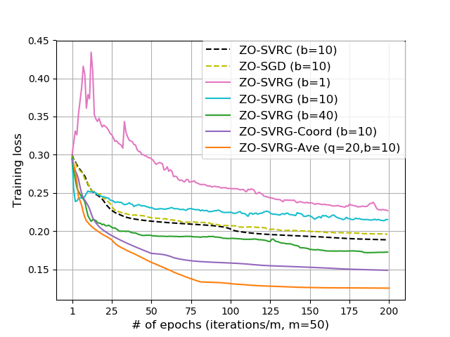
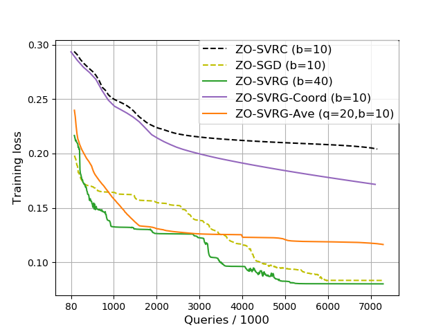
(a) Training loss versus iterations (b) Training loss versus function queries

Figure 2: Comparison of different ZO algorithms for the task of chemical material classification.

Table 2: Testing error for chemical material classification using $7.3\times 10^{6}$ function queries.

Method ZO-SGD [24] ZO-SVRC [26] ZO-SVRG ZO-SVRG-Coord ZO-SVRG-Ave # of epochs $14600$ $100$ $2920$ $50$ $365$ Error ($\%$) $12.56\%$ $23.70\%$ $11.18\%$ $20.67\%$ $15.26\%$

In Fig. 2, we present the training loss against the number of epochs (i.e., iterations divided by the epoch length $m=50$) and function queries. We compare our proposed algorithms ZO-SVRG, ZO-SVRG-Coord and ZO-SVRG-Ave with ZO-SGD [24] and ZO-SVRC [26]. Fig. 2-(a) presents the convergence trajectories of ZO algorithms as functions of the number of epochs, where ZO-SVRG is evaluated under different mini-batch sizes $b\in\{1,10,40\}$. We observe that the convergence error of ZO-SVRG decreases as $b$ increases, and for a small mini-batch size $b\leq 10$, ZO-SVRG likely converges to a neighborhood of a critical point as shown by Corollary 1. We also note that our proposed algorithms ZO-SVRG ($b=40$), ZO-SVRG-Coord and ZO-SVRG-Ave have faster convergence speeds (i.e., less iteration complexity) than the existing algorithms ZO-SGD and ZO-SVRC. Particularly, the use of multiple random direction samples in Avg-RandGradEst significantly accelerates ZO-SVRG since the error of order $O(1/b)$ is reduced to $O(1/(bq))$ (see Table 1), leading to a non-dominant factor versus $O(d/T)$ in the convergence rate of ZO-SVRG-Ave. Fig. 2-(b) presents the training loss against the number of function queries. For the same experiment, Table 2 shows the number of iterations and the testing error of algorithms studied in Fig. 2-(b) using $7.3\times 10^{6}$ function queries. We observe that the performance of CoordGradEst based algorithms (i.e., ZO-SVRC and ZO-SVRG-Coord) degrade due to the need of large number of function queries to construct coordinate-wise gradient estimates. By contrast, algorithms based on random gradient estimators (i.e., ZO-SGD, ZO-SVRG and ZO-SVRG-Ave) yield better both training and testing results, while ZO-SGD consumes an extremely large number of iterations ($14600$ epochs). As a result, ZO-SVRG ($b=40$) and ZO-SVRG-Ave achieve better tradeoffs between the iteration and the function query complexity.

Generation of adversarial examples from black-box DNNs

In image classification, adversarial examples refer to carefully crafted perturbations such that, when added to the natural images, are visually imperceptible but will lead the target model to misclassify. In the setting of ‘zeroth order’ attacks [2, 3, 35], the model parameters are hidden and acquiring its gradient is inadmissible. Only the model evaluations are accessible. We can then regard the task of generating a universal adversarial perturbation (to $n$ natural images) as an ZO optimization problem of the form (1). We elaborate on the problem formulation for generating adversarial examples in Appendix A.11.

We use a well-trained DNN on the MNIST handwritten digit classification task as the target black-box model, which achieves 99.4% test accuracy on natural examples. Two ZO optimization methods, ZO-SGD and ZO-SVRG-Ave, are performed in our experiment. Note that ZO-SVRG-Ave reduces to ZO-SVRG when $q=1$. We choose $n=10$ images from the same class, and set the same parameters $b=5$ and constant step size $30/d$ for both ZO methods, where $d=28\times 28$ is the image dimension. For ZO-SVRG-Ave, we set $m=10$ and vary the number of random direction samples $q\in\{10,20,30\}$. In Fig. 3, we show the black-box attack loss (against the number of epochs) as well as the least $\ell_{2}$ distortion of the successful (universal) adversarial perturbations. To reach the same attack loss (e.g., $7$ in our example), ZO-SVRG-Ave requires roughly $30\times$ ($q=10$), $77\times$ ($q=20$) and $380\times$ ($q=30$) more function evaluations than ZO-SGD. The sharp drop of attack loss in each method could be caused by the hinge-like loss as part of the total loss function, which turns to $0$ only if the attack becomes successful. Compared to ZO-SGD, ZO-SVRG-Ave offers a faster convergence to a more accurate solution, and its convergence trajectory is more stable as $q$ becomes larger (due to the reduced variance of Avg-RandGradEst). In addition, ZO-SVRG-Ave improves the $\ell_{2}$ distortion of adversarial examples compared to ZO-SGD (e.g., $30\%$ improvement when $q=30$). We present the corresponding adversarial examples in Appendix A.11.

Method	$\ell_{2}$ distortion
ZO-SGD	$5.22$
ZO-SVRG-Ave ($q=10$)	$4.91$ ($6\%$)
ZO-SVRG-Ave ($q=20$)	$3.91$ ($25\%$)
ZO-SVRG-Ave ($q=30$)	$3.67$ ($30\%$)

Figure 3: Comparison of ZO-SGD and ZO-SVRG-Ave for generation of universal adversarial perturbations from a black-box DNN. Left: Attack loss versus iterations. Right: $\ell_{2}$ distortion and improvement $(\%)$ with respect to ZO-SGD.

7 Conclusion

In this paper, we studied ZO-SVRG, a new ZO nonconvex optimization method. We presented new convergence results beyond the existing work on ZO nonconvex optimization. We show that ZO-SVRG improves the convergence rate of ZO-SGD from $O(1/\sqrt{T})$ to $O(1/{T})$ but suffers a new correction term of order $O(1/b)$. The is the side effect of combining a two-point random gradient estimators with SVRG. We then propose two accelerated variants of ZO-SVRG based on improved gradient estimators of reduced variances. We show an illuminating trade-off between the iteration and the function query complexity. Experimental results and theoretical analysis validate the effectiveness of our approaches compared to other state-of-the-art algorithms.

Appendix A Supplementary material

A.1 Zeroth-order (ZO) gradient estimators

With an abuse of notation, in this section let $f$ be an arbitrary function under assumptions A1 and A2. Lemma 1 shows the second-order statistics of RandGradEst.

Lemma 1

Suppose that Assumption A1 holds, and define $f_{\mu}=\mathbb{E}_{\mathbf{u}\in U_{\mathrm{b}}}[f(\mathbf{x}+\mu\mathbf{u})]$, where $U_{\mathrm{b}}$ is a uniform distribution over the unit Euclidean ball. Then RandGradEst yields:

1) $f_{\mu}$ is $L$-smooth, and

$$\nabla f_{\mu}(\mathbf{x})=\mathbb{E}_{\mathbf{u}}\left[\hat{\nabla}f(\mathbf{x})\right],$$ (17)

where $\mathbf{u}$ is drawn from the uniform distribution over the unit Euclidean sphere, and $\hat{\nabla}f(\mathbf{x})$ is given by RandGradEst.

2) For any $\mathbf{x}\in\mathbb{R}^{d}$,

$$|f_{\mu}(\mathbf{x})-f(\mathbf{x})|\leq\frac{L\mu^{2}}{2}$$ (18)

$$\|\nabla f_{\mu}(\mathbf{x})-\nabla f(\mathbf{x})\|_{2}^{2}\leq\frac{\mu^{2}L^{2}d^{2}}{4},$$ (19)

$$\frac{1}{2}\|\nabla f(\mathbf{x})\|_{2}^{2}-\frac{\mu^{2}L^{2}d^{2}}{4}\leq\|\nabla f_{\mu}(\mathbf{x})\|_{2}^{2}\leq 2\|\nabla f(\mathbf{x})\|_{2}^{2}+\frac{\mu^{2}L^{2}d^{2}}{2}.$$ (20)

3) For any $\mathbf{x}\in\mathbb{R}^{d}$,

$$\mathbb{E}_{\mathbf{u}}\left[\|\hat{\nabla}f(\mathbf{x})-\nabla f_{\mu}(\mathbf{x})\|_{2}^{2}\right]\leq\mathbb{E}_{\mathbf{u}}\left[\|\hat{\nabla}f(\mathbf{x})\|_{2}^{2}\right]\leq 2d\|\nabla f(\mathbf{x})\|_{2}^{2}+\frac{\mu^{2}L^{2}d^{2}}{2}.$$ (21)

Proof: First, by using [16, Lemma 4.1.a] (also see [36] and [13]), we immediately obtain that $f_{\mu}$ is $L_{\mu}$ smooth with $L_{\mu}\leq L$, and

$$\nabla f_{\mu}(\mathbf{x})=\mathbb{E}_{\mathbf{u}}\left[\frac{d}{\mu}f(\mathbf{x}+\mu\mathbf{u})\mathbf{u}\right].$$ (22)

Since $\mathbb{E}_{\mathbf{u}}[(d/\mu)f(\mathbf{x})\mathbf{u}]=0$, we obtain (17).

Next, we obtain (18)-(20) based on [16, Lemma 4.1.b]. Moreover, we have

$$\|\nabla f_{\mu}(\mathbf{x})\|_{2}^{2}= \|\nabla f_{\mu}(\mathbf{x})-\nabla f(\mathbf{x})+\nabla f(\mathbf{x})\|_{2}^{2}$$

$$\leq 2\|\nabla f(\mathbf{x})\|_{2}^{2}+2\|\nabla f_{\mu}(\mathbf{x})-\nabla f(\mathbf{x})\|_{2}^{2}$$

$$\overset{\eqref{eq: dist_smooth_true}}{\leq} 2\|\nabla f(\mathbf{x})\|_{2}^{2}+\frac{\mu^{2}d^{2}L^{2}}{2},$$ (23)

where the first inequality holds due to Lemma 6. Similarly, we have

$$\|\nabla f(\mathbf{x})\|_{2}^{2}=\|\nabla f_{\mu}(\mathbf{x})+\nabla f(\mathbf{x})-\nabla f_{\mu}(\mathbf{x})\|_{2}^{2}\overset{\eqref{eq: dist_smooth_true}}{\leq}2\|\nabla f_{\mu}(\mathbf{x})\|_{2}^{2}+\frac{\mu^{2}d^{2}L^{2}}{2},$$ (24)

which yields

$$\|\nabla f_{\mu}(\mathbf{x})\|_{2}^{2}\geq\frac{1}{2}\|\nabla f(\mathbf{x})\|_{2}^{2}-\frac{\mu^{2}L^{2}d^{2}}{4}.$$ (25)

In (21), the first inequality holds due to (17) and $\mathbb{E}[\|\mathbf{a}-\mathbb{E}[\mathbf{a}]\|_{2}^{2}]\leq\mathbb{E}[\|\mathbf{a}\|_{2}^{2}]$ for a random variable $\mathbf{a}$. And the second inequality of (21) holds due to [16, Lemma 4.1.b]. The proof is now complete. $\square$

In Lemma 2, we show the properties of Avg-RandGradEst.

Lemma 2

Following the conditions of Lemma 1, then Avg-RandGradEst yields:

1) For any $\mathbf{x}\in\mathbb{R}^{d}$

$$\nabla f_{\mu}(\mathbf{x})=\mathbb{E}\left[\hat{\nabla}f(\mathbf{x})\right],$$ (26)

where $\hat{\nabla}f(\mathbf{x})$ is given by Avg-RandGradEst.

2) For any $\mathbf{x}\in\mathbb{R}^{d}$

$$\mathbb{E}\left[\|\hat{\nabla}f(\mathbf{x})-\nabla f_{\mu}(\mathbf{x})\|_{2}^{2}\right]\leq\mathbb{E}\left[\|\hat{\nabla}f(\mathbf{x})\|_{2}^{2}\right]\leq 2\left(1+\frac{d}{q}\right)\|\nabla f(\mathbf{x})\|_{2}^{2}+\left(1+\frac{1}{q}\right)\frac{\mu^{2}L^{2}d^{2}}{2}.$$ (27)

Proof: Since $\{\mathbf{u}_{i}\}_{i=1}^{q}$ are i.i.d. random vectors, we have

$$\mathbb{E}\left[\hat{\nabla}f(\mathbf{x})\right]=\mathbb{E}_{\mathbf{u}_{i}}\left[\hat{\nabla}f(\mathbf{x};\mathbf{u}_{i})\right]\overset{\eqref{eq: smooth_est_grad}}{=}\nabla f_{\mu}(\mathbf{x}),$$ (28)

where $\hat{\nabla}f(\mathbf{x};\mathbf{u}_{i})\mathrel{\mathop{:}}=\frac{d}{\mu}[f(\mathbf{x}+\mu\mathbf{u}_{i})-f(\mathbf{x})]\mathbf{u}_{i}$.

In (27), the first inequality holds due to (26) and $\mathbb{E}[\|\mathbf{a}-\mathbb{E}[\mathbf{a}]\|_{2}^{2}]\leq\mathbb{E}[\|\mathbf{a}\|_{2}^{2}]$ for a random variable $\mathbf{a}$. Next, we bound the second moment of $\hat{\nabla}f(\mathbf{x})$

$$\mathbb{E}\left[\left\|\hat{\nabla}f(\mathbf{x})\right\|_{2}^{2}\right]= \mathbb{E}\left[\left\|\frac{1}{q}\sum_{i=1}^{q}\left(\hat{\nabla}f(\mathbf{x};\mathbf{u}_{i})-{\nabla}f_{\mu}(\mathbf{x})\right)+{\nabla}f_{\mu}(\mathbf{x})\right\|_{2}^{2}\right]$$

$$= \left\|{\nabla}f_{\mu}(\mathbf{x})\right\|_{2}^{2}+\mathbb{E}\left[\left\|\frac{1}{q}\sum_{i=1}^{q}\left(\hat{\nabla}f(\mathbf{x};\mathbf{u}_{i})-{\nabla}f_{\mu}(\mathbf{x})\right)\right\|_{2}^{2}\right]$$

$$= \left\|{\nabla}f_{\mu}(\mathbf{x})\right\|_{2}^{2}+\frac{1}{q}\mathbb{E}\left[\left\|\hat{\nabla}f(\mathbf{x};{\color[rgb]{0,0,0}\mathbf{u}_{1}})-{\nabla}f_{\mu}(\mathbf{x})\right\|_{2}^{2}\right],$$ (29)

where the expectation is taken with respect to i.i.d. random vectors $\{\mathbf{u}_{i}\}$, and we have used the fact that $\mathbb{E}[\|\hat{\nabla}f(\mathbf{x};\mathbf{u}_{i})-{\nabla}f_{\mu}(\mathbf{x})\|_{2}^{2}]=\mathbb{E}[\|\hat{\nabla}f(\mathbf{x};\mathbf{u}_{1})-{\nabla}f_{\mu}(\mathbf{x})\|_{2}^{2}]$ for any $i$. Substituting (20) and (21) into (29), we obtain (27). $\square$

In Lemma 3, we demonstrate the properties of CoordGradEst.

Lemma 3

Let Assumption A1 hold and define $f_{\mu_{\ell}}(\mathbf{x})=\mathbb{E}_{u\sim U[-\mu_{\ell},\mu_{\ell}]}f(\mathbf{x}+u\mathbf{e}_{\ell})$, where $U[-\mu_{\ell},\mu_{\ell}]$ denotes the uniform distribution at the interval $[-\mu_{\ell},\mu_{\ell}]$. We then have:

1) $f_{\mu_{\ell}}$ is L-smooth, and

$${\hat{\nabla}}f(\mathbf{x})=\sum_{\ell=1}^{d}\frac{\partial f_{\mu_{\ell}}(\mathbf{x})}{\partial x_{\ell}}\mathbf{e}_{\ell},$$ (30)

where ${\hat{\nabla}}f(\mathbf{x})$ is defined by CoordGradEst, and $\partial f/\partial x_{\ell}$ denotes the partial derivative with respect to the $\ell$th coordinate.

2) For $\ell\in[d]$,

$$|f_{\mu_{\ell}}(\mathbf{x})-f(\mathbf{x})|\leq\frac{L\mu_{\ell}^{2}}{2},$$ (31)

$$\left|\frac{\partial f_{\mu_{\ell}}(\mathbf{x})}{\partial x_{\ell}}-\frac{\partial f(\mathbf{x})}{\partial x_{\ell}}\right|\leq\frac{L\mu_{\ell}}{2}.$$ (32)

3) For $\ell\in[d]$,

$$\left\|\hat{\nabla}f(\mathbf{x})-\nabla f(\mathbf{x})\right\|_{2}^{2}\leq\frac{L^{2}d}{4}\sum_{\ell=1}^{d}\mu_{\ell}^{2}.$$ (33)

Proof: For the $\ell$th coordinate, it is known from [7, Lemma 6] that $f_{\mu_{\ell}}$ is $L$-smooth and

$$\frac{\partial f_{\mu_{\ell}}(\mathbf{x})}{\partial x_{\ell}}=\frac{f(\mathbf{x}+\mu_{\ell}\mathbf{e}_{\ell})-f(\mathbf{x}-\mu_{\ell}\mathbf{e}_{\ell})}{2\mu_{\ell}}.$$ (34)

Based on (34) and the definition of CoordGradEst, we then obtain (30).

The inequalities (31) and (32) have been proved by [7, Lemma 6].

Based on (30) and (32), we have

$$\left\|\hat{\nabla}f(\mathbf{x})-\nabla f(\mathbf{x})\right\|_{2}^{2}\overset{\eqref{eq: grad_f_smooth_coord_all}}{=}\left\|\sum_{\ell=1}^{d}\left(\frac{\partial f_{\mu_{\ell}}(\mathbf{x})}{\partial x_{\ell}}-\frac{\partial f(\mathbf{x})}{\partial x_{\ell}}\right)\mathbf{e}_{\ell}\right\|_{2}^{2}$$

$$\leq d\sum_{\ell=1}^{d}\left\|\frac{\partial f_{\mu_{\ell}}(\mathbf{x})}{\partial x_{\ell}}-\frac{\partial f(\mathbf{x})}{\partial x_{\ell}}\right\|_{2}^{2}\leq\frac{L^{2}d}{4}\sum_{\ell=1}^{d}\mu_{\ell}^{2},$$

where the first inequality holds due to Lemma 6 in Sec. A.9. The proof is now complete. $\square$

A.2 Control variates

The gradient blending in Step 6 of SVRG (Algorithm 1) can be interpreted using control variate [28, 29, 30]. If we view $\hat{\mathbf{g}}_{0}\mathrel{\mathop{:}}=\nabla f_{\mathcal{I}}(\mathbf{x})$ as the raw gradient estimate at $\mathbf{x}$, and $\mathbf{c}\mathrel{\mathop{:}}=\nabla f_{\mathcal{I}}(\hat{\mathbf{x}})$ as a control variate satisfying $\mathbb{E}[\mathbf{c}]=\nabla f(\hat{\mathbf{x}})$, then the gradient blending (2) becomes a gradient estimate modified by a control variate, $\hat{\mathbf{g}}=\hat{\mathbf{g}}_{0}-(\mathbf{c}-\mathbb{E}[\mathbf{c}])$. Here $\hat{\mathbf{g}}$ has the same expectation as $\hat{\mathbf{g}}_{0}$, i.e., $\mathbb{E}[\hat{\mathbf{g}}]=\mathbb{E}[\hat{\mathbf{g}}_{0}]=\nabla f(\mathbf{x})$, however, has a lower variance when $\mathbf{c}$ is positively correlated with $\mathbf{g}_{0}$ (see a detailed analysis as below).

Consider the following gradient estimator,

$$\hat{\mathbf{g}}=\hat{\mathbf{g}}_{0}-\eta(\mathbf{c}-\mathbb{E}[\mathbf{c}]),$$ (35)

where $\hat{\mathbf{g}}_{0}$ is a given (raw) gradient estimate, $\eta$ is an unknown coefficient, and $\mathbf{c}$ is a control variate. It is clear that $\hat{\mathbf{g}}$ has the same expectation as $\hat{\mathbf{g}}_{0}$. We then study the effect of $\mathbf{c}$ on the variance of $\hat{\mathbf{g}}$,

$$\operatorname{tr}(\operatorname{cov}(\hat{\mathbf{g}}))=\operatorname{tr}(\operatorname{cov}({\hat{\mathbf{g}}_{0}}))+\eta^{2}\operatorname{tr}(\operatorname{cov}(\mathbf{c}))-2\eta\operatorname{tr}(\operatorname{cov}(\hat{\mathbf{g}}_{0},\mathbf{c})),$$ (36)

where $\operatorname{tr}(\cdot)$ denotes the trace operator, and $\operatorname{cov}(\cdot)$ is the covariance operator. When $\eta=\frac{\operatorname{tr}(\operatorname{cov}(\hat{\mathbf{g}}_{0},\mathbf{c}))}{\operatorname{tr}(\operatorname{cov}(\mathbf{c}))}$, the variance of $\hat{\mathbf{g}}$ in (36) is then minimized, leading to

$$\operatorname{tr}(\operatorname{cov}(\hat{\mathbf{g}}))=\operatorname{tr}(\operatorname{cov}(\hat{\mathbf{g}}_{0}))\left(1-\rho(\hat{\mathbf{g}}_{0},\mathbf{c})^{2}\right),$$ (37)

where $\rho(\hat{\mathbf{g}}_{0},\mathbf{c})=\frac{\operatorname{tr}(\operatorname{cov}(\hat{\mathbf{g}}_{0},\mathbf{c}))}{\sqrt{\operatorname{tr}(\operatorname{cov}(\hat{\mathbf{g}}_{0}))}\sqrt{\operatorname{tr}(\operatorname{cov}(\mathbf{c}))}}$. In (37), $\rho(\hat{\mathbf{g}}_{0},\mathbf{c})$ indicates the correlation strength between $\hat{\mathbf{g}}_{0}$ and $\mathbf{c}$. Therefore, the gradient estimate $\hat{\mathbf{g}}$ has a smaller variance than $\hat{\mathbf{g}}_{0}$ when the control variate $\mathbf{c}$ is positively correlated with the latter. Moreover, if $\mathbf{c}$ is chosen similar to $\hat{\mathbf{g}}$, then $\eta$ would be close to 1.

A.3 Proof of Proposition 1

In Algorithm 2, we recall that the mini-batch $\mathcal{I}$ is chosen uniformly randomly (with replacement). It is known from Lemma 4 and Lemma 5 that

$$\mathbb{E}_{\mathcal{I}_{k}}[\hat{\nabla}f_{\mathcal{I}_{k}}(\mathbf{x}_{k}^{s})-\hat{\nabla}f_{\mathcal{I}_{k}}(\mathbf{x}_{0}^{s})]=\hat{\nabla}f(\mathbf{x}_{k}^{s})-\hat{\nabla}f(\mathbf{x}_{0}^{s}).$$ (38)

We then rewrite $\hat{\mathbf{v}}_{k}^{s}$ as

$$\hat{\mathbf{v}}_{k}^{s}= \hat{\nabla}f_{\mathcal{I}_{k}}(\mathbf{x}_{k}^{s})-\hat{\nabla}f_{\mathcal{I}_{k}}(\mathbf{x}_{0}^{s})-\mathbb{E}_{\mathcal{I}_{k}}[\hat{\nabla}f_{\mathcal{I}_{k}}(\mathbf{x}_{k}^{s})-\hat{\nabla}f_{\mathcal{I}_{k}}(\mathbf{x}_{0}^{s})]+\hat{\nabla}f(\mathbf{x}_{k}^{s}).$$ (39)

Taking the expectation of $\|\mathbf{v}_{k}^{s}\|_{2}^{2}$ with repsect to all the random variables, we have

$$\mathbb{E}\left[\|\hat{\mathbf{v}}_{k}^{s}\|_{2}^{2}\right]\leq 2\mathbb{E}\left[\|\hat{\nabla}f_{\mathcal{I}_{k}}(\mathbf{x}_{k}^{s})-\hat{\nabla}f_{\mathcal{I}_{k}}(\mathbf{x}_{0}^{s})-\mathbb{E}_{\mathcal{I}_{k}}[\hat{\nabla}f_{\mathcal{I}_{k}}(\mathbf{x}_{k}^{s})-\hat{\nabla}f_{\mathcal{I}_{k}}(\mathbf{x}_{0}^{s})]\|_{2}^{2}\right]+2\mathbb{E}\left[\|\hat{\nabla}f(\mathbf{x}_{k}^{s})\|_{2}^{2}\right]$$

$$\leq 2\mathbb{E}\left[\|\hat{\nabla}f_{\mathcal{I}_{k}}(\mathbf{x}_{k}^{s})-\hat{\nabla}f_{\mathcal{I}_{k}}(\mathbf{x}_{0}^{s})-\mathbb{E}_{\mathcal{I}_{k}}[\hat{\nabla}f_{\mathcal{I}_{k}}(\mathbf{x}_{k}^{s})-\hat{\nabla}f_{\mathcal{I}_{k}}(\mathbf{x}_{0}^{s})]\|_{2}^{2}\right]$$

$$+4d\mathbb{E}\left[\|\nabla f(\mathbf{x}_{k}^{s})\|_{2}^{2}\right]+\mu^{2}d^{2}L^{2},$$ (40)

where the first inequality holds due to Lemma 6, and the second inequality holds due to (21). Based on (38), we note that the following holds

$$\sum_{i=1}^{n}\left\{\hat{\nabla}f_{i}(\mathbf{x}_{k}^{s})-\hat{\nabla}f_{i}(\mathbf{x}_{k}^{s})-\mathbb{E}_{\mathcal{I}_{k}}[\hat{\nabla}f_{\mathcal{I}_{k}}(\mathbf{x}_{k}^{s})-\hat{\nabla}f_{\mathcal{I}_{k}}(\mathbf{x}_{0}^{s})]\right\}$$

$$= n(\hat{\nabla}f(\mathbf{x}_{k}^{s})-\hat{\nabla}f(\mathbf{x}_{0}^{s}))-n(\hat{\nabla}f(\mathbf{x}_{k}^{s})-\hat{\nabla}f(\mathbf{x}_{0}^{s}))=\mathbf{0}.$$ (41)

Based on (A.3) and applying Lemma 4 and 5, the first term at the right hand side (RHS) of (A.3) yields

$$\mathbb{E}\left[\|\hat{\nabla}f_{\mathcal{I}_{k}}(\mathbf{x}_{k}^{s})-\hat{\nabla}f_{\mathcal{I}_{k}}(\mathbf{x}_{0}^{s})-\mathbb{E}_{\mathcal{I}_{k}}[\hat{\nabla}f_{\mathcal{I}_{k}}(\mathbf{x}_{k}^{s})-\hat{\nabla}f_{\mathcal{I}_{k}}(\mathbf{x}_{0}^{s})]\|_{2}^{2}\right]$$

$$\leq \frac{\delta_{n}}{bn}\sum_{i=1}^{n}\mathbb{E}\left[\|\hat{\nabla}f_{i}(\mathbf{x}_{k}^{s})-\hat{\nabla}f_{i}(\mathbf{x}_{0}^{s})-(\hat{\nabla}f(\mathbf{x}_{k}^{s})-\hat{\nabla}f(\mathbf{x}_{0}^{s}))\|_{2}^{2}\right]$$

$$= \mathbb{E}\left[\frac{\delta_{n}}{b}\left(\frac{1}{n}\sum_{i=1}^{n}\|\hat{\nabla}f_{i}(\mathbf{x}_{k}^{s})-\hat{\nabla}f_{i}(\mathbf{x}_{0}^{s})\|_{2}^{2}-\|\hat{\nabla}f(\mathbf{x}_{k}^{s})-\hat{\nabla}f(\mathbf{x}_{0}^{s})\|_{2}^{2}\right)\right]$$

$$\leq \frac{\delta_{n}}{bn}\sum_{i=1}^{n}\mathbb{E}\left[\|\hat{\nabla}f_{i}(\mathbf{x}_{k}^{s})-\hat{\nabla}f_{i}(\mathbf{x}_{0}^{s})\|_{2}^{2}\right].$$ (42)

where the first inequality holds due to Lemma 4 and 5 (taking the expectation with respect to mini-batch $\mathcal{I}$), we define $\delta_{n}$ as

$$\delta_{n}=\left\{\begin{array}[]{ll}1&\text{if $\mathcal{I}$ contains i.i.d. samples with replacement (Lemma\,\ref{lemma: minibatch})}\\ I(b<n)&\text{if $\mathcal{I}$ contains samples without replacement (Lemma\,\ref{lemma: minibatch_noReplace})},\end{array}\right.$$ (45)

$I(b<n)=1$ if $b<n$ and $0$ otherwise, and the second equality in (A.3) holds since $\frac{1}{n}\sum_{i=1}^{n}\|\mathbf{x}_{i}-\mathbf{a}\|_{2}^{2}=\frac{1}{n}\sum_{i=1}^{n}\|\mathbf{x}_{i}\|_{2}^{2}-\|\mathbf{a}\|_{2}^{2}$ when $\mathbf{a}=\frac{1}{n}\sum_{i=1}^{n}\mathbf{x}_{i}$.

Substituting (A.3) into (A.3), we obtain

$$\mathbb{E}\left[\|\hat{\mathbf{v}}_{k}^{s}\|_{2}^{2}\right]\leq \frac{2\delta_{n}}{bn}\sum_{i=1}^{n}\mathbb{E}\left[\|\hat{\nabla}f_{i}(\mathbf{x}_{k}^{s})-\hat{\nabla}f_{i}(\mathbf{x}_{0}^{s})\|_{2}^{2}\right]+4d\mathbb{E}\left[\|\nabla f(\mathbf{x}_{k}^{s})\|_{2}^{2}\right]+\mu^{2}d^{2}L^{2}.$$ (46)

Similar to Lemma 1, we introduce a smoothing function $f_{i,\mu}$ of $f_{i}$, and continue to bound the first term at the right hand side (RHS) of (46). This yields

$$\mathbb{E}\left[\|\hat{\nabla}f_{i}(\mathbf{x}_{k}^{s})-\hat{\nabla}f_{i}(\mathbf{x}_{0}^{s})\|_{2}^{2}\right]$$

$$\overset{\eqref{eq: sum_exp_bd}}{\leq} 3\mathbb{E}\left[\|\hat{\nabla}f_{i}(\mathbf{x}_{k}^{s})-\nabla f_{i,\mu}(\mathbf{x}_{k}^{s})\|_{2}^{2}\right]+3\mathbb{E}\left[\|\hat{\nabla}f_{i,\mu}(\mathbf{x}_{0}^{s})-\nabla f_{i}(\mathbf{x}_{0}^{s})\|_{2}^{2}\right]$$

$$+3\mathbb{E}\left[\|\nabla f_{i,\mu}(\mathbf{x}_{k}^{s})-\nabla f_{i,\mu}(\mathbf{x}_{0}^{s})\|_{2}^{2}\right]$$

$$\overset{\eqref{eq: second_moment_grad_random}}{\leq} 6d\mathbb{E}[\|\nabla f_{i}(\mathbf{x}_{k}^{s})\|_{2}^{2}]+6d\mathbb{E}[\|\nabla f_{i}(\mathbf{x}_{0}^{s})\|_{2}^{2}]+3L^{2}d^{2}\mu^{2}+3\mathbb{E}\left[\|\nabla f_{i,\mu}(\mathbf{x}_{k}^{s})-\nabla f_{i,\mu}(\mathbf{x}_{0}^{s})\|_{2}^{2}\right].$$ (47)

Since both $f_{i}$ and $f_{i,\mu}$ are $L$-smooth (A1 and Lemma 1), we have

$$\mathbb{E}\left[\|\nabla f_{i,\mu}(\mathbf{x}_{k}^{s})-\nabla f_{i,\mu}(\mathbf{x}_{0}^{s})\|_{2}^{2}\right]\leq L^{2}\mathbb{E}\left[\|\mathbf{x}_{k}^{s}-\mathbf{x}_{0}^{s}\|_{2}^{2}\right],$$ (48)

$$\mathbb{E}\left[\|\nabla f_{i}(\mathbf{x}_{0}^{s})\|_{2}^{2}\right]\leq 2\mathbb{E}\left[\|\nabla f_{i}(\mathbf{x}_{0}^{s})-\nabla f_{i}(\mathbf{x}_{k}^{s})\|_{2}^{2}\right]+2\mathbb{E}\left[\|\nabla f_{i}(\mathbf{x}_{k}^{s})\|_{2}^{2}\right]$$

$$\hskip 65.04256pt\leq 2L^{2}\mathbb{E}\left[\|\mathbf{x}_{0}^{s}-\mathbf{x}_{k}^{s}\|_{2}^{2}\right]+2\mathbb{E}\left[\|\nabla f_{i}(\mathbf{x}_{k}^{s})\|_{2}^{2}\right].$$ (49)

Substituting (48) and (49) into (A.3), we obtain

$$\mathbb{E}\left[\|\hat{\nabla}f_{i}(\mathbf{x}_{k}^{s})-\hat{\nabla}f_{i}(\mathbf{x}_{0}^{s})\|_{2}^{2}\right]$$

$$\leq 18d\mathbb{E}[\|\nabla f_{i}(\mathbf{x}_{k}^{s})\|_{2}^{2}]+(12d+3)L^{2}\mathbb{E}\left[\|\mathbf{x}_{0}^{s}-\mathbf{x}_{k}^{s}\|_{2}^{2}\right]+3L^{2}d^{2}\mu^{2}$$

$$\leq 36d\mathbb{E}\left[\|\nabla f_{i}(\mathbf{x}_{k}^{s})-\nabla f(\mathbf{x}_{k}^{s})\|_{2}^{2}\right]+36d\mathbb{E}\left[\|\nabla f(\mathbf{x}_{k}^{s})\|_{2}^{2}\right]$$

$$+(12d+3)L^{2}\mathbb{E}\left[\|\mathbf{x}_{0}^{s}-\mathbf{x}_{k}^{s}\|_{2}^{2}\right]+3L^{2}d^{2}\mu^{2}$$

$$\leq 36d\sigma^{2}+36d\mathbb{E}\left[\|\nabla f(\mathbf{x}_{k}^{s})\|_{2}^{2}\right]+(12d+3)L^{2}\mathbb{E}\left[\|\mathbf{x}_{0}^{s}-\mathbf{x}_{k}^{s}\|_{2}^{2}\right]+3L^{2}d^{2}\mu^{2},$$ (50)

where the last inequality holds due to Assumption A2.

Substituting (A.3) into (46), we have

$$\mathbb{E}\left[\|\hat{\mathbf{v}}_{k}^{s}\|_{2}^{2}\right]\leq \frac{6\delta_{n}(4d+1)L^{2}}{b}\mathbb{E}\left[\|\mathbf{x}_{0}^{s}-\mathbf{x}_{k}^{s}\|_{2}^{2}\right]$$

$$+\left(4d+\frac{72d\delta_{n}}{b}\right)\mathbb{E}\left[\|\nabla f(\mathbf{x}_{k}^{s})\|_{2}^{2}\right]+\left(1+\frac{6\delta_{n}}{b}\right)d^{2}L^{2}\mu^{2}+\frac{72d\sigma^{2}\delta_{n}}{b}.$$ (51)

The proof is now complete. $\square$

A.4 Proof of Theorem 1

Since $f_{\mu}$ is $L$-smooth (Lemma 1), from Lemma 7 in Sec. A.9 we have

$$f_{\mu}(\mathbf{x}_{k+1}^{s})\leq f_{\mu}(\mathbf{x}_{k}^{s})+\langle\nabla f_{\mu}(\mathbf{x}_{k}^{s}),\mathbf{x}_{k+1}^{s}-\mathbf{x}_{k}^{s}\rangle+\frac{L}{2}\|x_{k+1}^{s}-\mathbf{x}_{k}^{s}\|_{2}^{2}$$

$$= f_{\mu}(\mathbf{x}_{k}^{s})-\eta_{k}\langle\nabla f_{\mu}(\mathbf{x}_{k}^{s}),\hat{\mathbf{v}}_{k}^{s}\rangle+\frac{L}{2}\eta_{k}^{2}\|\hat{\mathbf{v}}_{k}^{s}\|_{2}^{2},$$ (52)

where the last equality holds due to $\mathbf{x}_{k+1}^{s}=\mathbf{x}_{k}^{s}-\eta_{k}\hat{\mathbf{v}}_{k}^{s}$. Since $\mathbf{x}_{k}^{s}$ and $\mathbf{x}_{0}^{s}$ are independent of $\mathcal{I}_{k}$ and random directions $\mathbf{u}$ used for ZO gradient estimates, from (17) we obtain

$$\mathbb{E}_{\mathbf{u},\mathcal{I}_{k}}\left[\hat{\mathbf{v}}_{k}^{s}\right]= \mathbb{E}_{\mathbf{u},\mathcal{I}_{k}}\left[\hat{\nabla}f_{{\mathcal{I}}_{k}}({\mathbf{x}}_{k}^{s})-\hat{\nabla}f_{{\mathcal{I}}_{k}}({\mathbf{x}}_{0}^{s})+\hat{\nabla}f(\mathbf{x}_{0}^{s})\right]$$

$$= \nabla f_{\mu}(\mathbf{x}_{k}^{s})+\nabla f_{\mu}(\mathbf{x}_{0}^{s})-\nabla f_{\mu}(\mathbf{x}_{0}^{s})=\nabla f_{\mu}(\mathbf{x}_{k}^{s}).$$ (53)

Combining (A.4) and (A.4), we have

$$\mathbb{E}\left[f_{\mu}(\mathbf{x}_{k+1}^{s})\right]\leq \mathbb{E}\left[f_{\mu}(\mathbf{x}_{k}^{s})\right]-\eta_{k}\mathbb{E}\left[\|\nabla f_{\mu}(\mathbf{x}_{k}^{s})\|_{2}^{2}\right]+\frac{L}{2}\eta_{k}^{2}\mathbb{E}\left[\|\hat{\mathbf{v}}_{k}^{s}\|_{2}^{2}\right],$$ (54)

where the expectation is taken with respect to all random variables.

At RHS of (54), the upper bound on $\mathbb{E}\left[\|\hat{\mathbf{v}}_{k}^{s}\|_{2}^{2}\right]$ is given by Proposition 1,

$$\mathbb{E}[\|\hat{\mathbf{v}}_{k}^{s}\|_{2}^{2}]\leq \frac{4(b+18{\color[rgb]{0,0,0}\delta_{n}})d}{b}\mathbb{E}\left[\|\nabla f(\mathbf{x}_{k}^{s})\|_{2}^{2}\right]+\frac{6(4d+1)L^{2}{\color[rgb]{0,0,0}\delta_{n}}}{b}\mathbb{E}\left[\|\mathbf{x}_{k}^{s}-\mathbf{x}_{0}^{s}\|_{2}^{2}\right]$$

$$+\frac{(6{\color[rgb]{0,0,0}\delta_{n}}+b)L^{2}d^{2}\mu^{2}}{b}+\frac{72d\sigma^{2}{\color[rgb]{0,0,0}\delta_{n}}}{b}.$$ (55)

In (A.4), we further bound $\mathbb{E}\left[\|\mathbf{x}_{k+1}^{s}-\mathbf{x}_{0}^{s}\|_{2}^{2}\right]$ as

$$\mathbb{E}\left[\|\mathbf{x}_{k+1}^{s}-\mathbf{x}_{0}^{s}\|_{2}^{2}\right]=\mathbb{E}\left[\|\mathbf{x}_{k+1}^{s}-\mathbf{x}_{k}^{s}+\mathbf{x}_{k}^{s}-\mathbf{x}_{0}^{s}\|_{2}^{2}\right]$$

$$= \eta_{k}^{2}\mathbb{E}\left[\|\hat{\mathbf{v}}_{k}^{s}\|_{2}^{2}\right]+\mathbb{E}\left[\|\mathbf{x}_{k}^{s}-\mathbf{x}_{0}^{s}\|_{2}^{2}\right]-2\eta_{k}\mathbb{E}\left[\langle\hat{\mathbf{v}}_{k}^{s},\mathbf{x}_{k}^{s}-\mathbf{x}_{0}^{s}\rangle\right]$$

$$\overset{\eqref{eq: E_uIk_v}}{=} \eta_{k}^{2}\mathbb{E}\left[\|\hat{\mathbf{v}}_{k}^{s}\|_{2}^{2}\right]+\mathbb{E}\left[\|\mathbf{x}_{k}^{s}-\mathbf{x}_{0}^{s}\|_{2}^{2}\right]-2\eta_{k}\mathbb{E}\left[\langle\nabla f_{\mu}(\mathbf{x}_{k}^{s}),\mathbf{x}_{k}^{s}-\mathbf{x}_{0}^{s}\rangle\right]$$

$$\leq \eta_{k}^{2}\mathbb{E}\left[\|\hat{\mathbf{v}}_{k}^{s}\|_{2}^{2}\right]+\mathbb{E}\left[\|\mathbf{x}_{k}^{s}-\mathbf{x}_{0}^{s}\|_{2}^{2}\right]+2\eta_{k}\mathbb{E}\left[\frac{1}{2\beta_{k}}\|\nabla f_{\mu}(\mathbf{x}_{k}^{s})\|_{2}^{2}+\frac{\beta_{k}}{2}\|\mathbf{x}_{k}^{s}-\mathbf{x}_{0}^{s}\|_{2}^{2}\right],$$ (56)

where $\beta_{k}$ is a positive coefficient, and the last inequality holds since $\langle\mathbf{a},\mathbf{b}\rangle\leq\frac{\beta\|\mathbf{a}\|_{2}^{2}+(1/\beta)\|\mathbf{b}\|_{2}^{2}}{2}$ for any $\mathbf{a}$ and $\mathbf{b}$, and $\beta>0$.

Now with (A.4) and (A.4) at hand, we introduce a Lyapunov function [20] with respect to $f_{\mu}$,

$$R_{k}^{s}=\mathbb{E}\left[f_{\mu}(\mathbf{x}_{k}^{s})+c_{k}\|\mathbf{x}_{k}^{s}-\mathbf{x}_{0}^{s}\|_{2}^{2}\right],$$ (57)

for some $c_{k}>0$. Substituting (54) and (A.4) into $R_{k+1}^{s}$, we obtain

$$R_{k+1}^{s}= \mathbb{E}\left[f_{\mu}(\mathbf{x}_{k+1}^{s})+c_{k+1}\|\mathbf{x}_{k+1}^{s}-\mathbf{x}_{0}^{s}\|_{2}^{2}\right]$$

$$\leq \mathbb{E}\left[f_{\mu}(\mathbf{x}_{k}^{s})-\eta_{k}\|\nabla f_{\mu}(\mathbf{x}_{k}^{s})\|_{2}^{2}+\frac{L}{2}\eta_{k}^{2}\|\hat{\mathbf{v}}_{k}^{s}\|_{2}^{2}\right]$$

$$+\mathbb{E}\left[c_{k+1}\eta_{k}^{2}\|\hat{\mathbf{v}}_{k}^{s}\|_{2}^{2}+c_{k+1}\|\mathbf{x}_{k}^{s}-\mathbf{x}_{0}^{s}\|_{2}^{s}\right]$$

$$+\mathbb{E}\left[\frac{c_{k+1}\eta_{k}}{\beta_{k}}\|\nabla f_{\mu}(\mathbf{x}_{k}^{s})\|_{2}^{2}+c_{k+1}\beta_{k}\eta_{k}\|\mathbf{x}_{k}^{s}-\mathbf{x}_{0}^{s}\|_{2}^{2}\right]$$

$$= \mathbb{E}\left[f_{\mu}(\mathbf{x}_{k}^{s})\right]-\left(\eta_{k}-\frac{c_{k+1}\eta_{k}}{\beta_{k}}\right)\mathbb{E}\left[\|\nabla f_{\mu}(\mathbf{x}_{k}^{s})\|_{2}^{2}\right]$$

$$+\left(c_{k+1}+c_{k+1}\beta_{k}\eta_{k}\right)\mathbb{E}\left[\|\mathbf{x}_{k}^{s}-\mathbf{x}_{0}^{s}\|_{2}^{2}\right]+\left(\frac{L}{2}\eta_{k}^{2}+c_{k+1}\eta_{k}^{2}\right)\mathbb{E}\left[\|\hat{\mathbf{v}}_{k}^{s}\|_{2}^{2}\right].$$ (58)

Moreover, substituting (A.4) into (A.4), we have

$$R_{k+1}^{s}\leq \mathbb{E}\left[f_{\mu}(\mathbf{x}_{k}^{s})\right]-\left(\eta_{k}-\frac{c_{k+1}\eta_{k}}{\beta_{k}}\right)\mathbb{E}\left[\|\nabla f_{\mu}(\mathbf{x}_{k}^{s})\|_{2}^{2}\right]+\left(c_{k+1}+c_{k+1}\beta_{k}\eta_{k}\right)\mathbb{E}\left[\|\mathbf{x}_{k}^{s}-\mathbf{x}_{0}^{s}\|_{2}^{2}\right]$$

$$+\left(\frac{L}{2}\eta_{k}^{2}+c_{k+1}\eta_{k}^{2}\right)\frac{6(4d+1)L^{2}{\color[rgb]{0,0,0}\delta_{n}}}{b}\mathbb{E}\left[\|\mathbf{x}_{k}^{s}-\mathbf{x}_{0}^{s}\|_{2}^{2}\right]$$

$$+\left(\frac{L}{2}\eta_{k}^{2}+c_{k+1}\eta_{k}^{2}\right)\frac{4db+72d{\color[rgb]{0,0,0}\delta_{n}}}{b}\mathbb{E}\left[\|\nabla f(\mathbf{x}_{k}^{s})\|_{2}^{2}\right]$$

$$+\left(\frac{L}{2}\eta_{k}^{2}+c_{k+1}\eta_{k}^{2}\right)\frac{(6{\color[rgb]{0,0,0}\delta_{n}}+b)L^{2}d^{2}\mu^{2}+72d\sigma^{2}{\color[rgb]{0,0,0}\delta_{n}}}{b}.$$ (59)

Based on the definition of $c_{k}=c_{k+1}+\beta_{k}\eta_{k}c_{k+1}+\frac{6(4d+1)L^{2}{\color[rgb]{0,0,0}\delta_{n}}\eta_{k}^{2}}{b}c_{k+1}+\frac{3(4d+1)L^{3}{\color[rgb]{0,0,0}\delta_{n}}\eta_{k}^{2}}{b}$ and the definition of $R_{k}^{s}$ in (57), we can simplify the inequality (A.4) as

$$R_{k+1}^{s}\leq R_{k}^{s}-\left(\eta_{k}-\frac{c_{k+1}\eta_{k}}{\beta_{k}}\right)\mathbb{E}\left[\|\nabla f_{\mu}(\mathbf{x}_{k}^{s})\|_{2}^{2}\right]$$

$$+\left(\frac{L}{2}\eta_{k}^{2}+c_{k+1}\eta_{k}^{2}\right)\frac{4db+72d{\color[rgb]{0,0,0}\delta_{n}}}{b}\mathbb{E}\left[\|\nabla f(\mathbf{x}_{k}^{s})\|_{2}^{2}\right]$$

$$+\left(\frac{L}{2}\eta_{k}^{2}+c_{k+1}\eta_{k}^{2}\right)\frac{(6{\color[rgb]{0,0,0}\delta_{n}}+b)L^{2}d^{2}\mu^{2}+72d\sigma^{2}{\color[rgb]{0,0,0}\delta_{n}}}{b}$$

$$\overset{\eqref{eq: up_grad_fsmooth}}{\leq} R_{k}^{s}-\frac{1}{2}\left(\eta_{k}-\frac{c_{k+1}\eta_{k}}{\beta_{k}}\right)\mathbb{E}\left[\|\nabla f(\mathbf{x}_{k}^{s})\|_{2}^{2}\right]+\left(\eta_{k}-\frac{c_{k+1}\eta_{k}}{\beta_{k}}\right)\frac{\mu^{2}d^{2}L^{2}}{4}$$

$$+\left(\frac{L}{2}\eta_{k}^{2}+c_{k+1}\eta_{k}^{2}\right)\frac{4db+72d{\color[rgb]{0,0,0}\delta_{n}}}{b}\mathbb{E}\left[\|\nabla f(\mathbf{x}_{k}^{s})\|_{2}^{2}\right]$$

$$+\left(\frac{L}{2}\eta_{k}^{2}+c_{k+1}\eta_{k}^{2}\right)\frac{(6{\color[rgb]{0,0,0}\delta_{n}}+b)L^{2}d^{2}\mu^{2}+72d\sigma^{2}{\color[rgb]{0,0,0}\delta_{n}}}{b}$$

$$= R_{k}^{s}-\gamma_{k}\mathbb{E}\left[\|\nabla f(\mathbf{x}_{k}^{s})\|_{2}^{2}\right]+\chi_{k},$$ (60)

where $\gamma_{k}$ and $\chi_{k}$ are coefficients given by

$$\gamma_{k}=\frac{1}{2}\left(1-\frac{c_{k+1}}{\beta_{k}}\right)\eta_{k}-\left(\frac{L}{2}+c_{k+1}\right)\frac{4db+72d{\color[rgb]{0,0,0}\delta_{n}}}{b}\eta_{k}^{2},$$ (61)

$$\chi_{k}=\left(\frac{L}{2}+c_{k+1}\right)\frac{(6{\color[rgb]{0,0,0}\delta_{n}}+b)L^{2}d^{2}\mu^{2}+72d\sigma^{2}{\color[rgb]{0,0,0}\delta_{n}}}{b}\eta_{k}^{2}+\left(1-\frac{c_{k+1}}{\beta_{k}}\right)\frac{\mu^{2}d^{2}L^{2}}{4}\eta_{k}.$$ (62)

In the second inequality of (A.4), we have used the fact that $1-\frac{c_{k+1}}{\beta_{k}}>0$. This holds for some parameter $\eta_{k}$ under the condition that $\gamma_{k}>0$. Even if $1-\frac{c_{k+1}}{\beta_{k}}<0$ (relaxing the condition $\gamma_{k}>0$), a similar inequality can be obtained using the upper bound of $\|\nabla f_{\mu}(\mathbf{x}_{k}^{s})\|_{2}^{2}$ in (20). Therefore, without loss of generality, we consider $1-\frac{c_{k+1}}{\beta_{k}}>0$.

Taking a telescopic sum for (A.4), we obtain

$$R_{m}^{s}\leq R_{0}^{s}-\sum_{k=0}^{m-1}\gamma_{k}\mathbb{E}\left[\|\nabla f(\mathbf{x}_{k}^{s})\|_{2}^{2}\right]+\chi_{m},$$ (63)

where $\chi_{m}=\sum_{k=0}^{m-1}\chi_{k}$. It is known from (57) that

$$R_{0}^{s}=\mathbb{E}\left[f_{\mu}(\mathbf{x}_{0}^{s})\right],\quad R_{m}^{s}=\mathbb{E}\left[f_{\mu}(\mathbf{x}_{m}^{s})\right],$$ (64)

where the last equality used the fact that $c_{m}=0$. Since $\tilde{\mathbf{x}}_{s-1}=\mathbf{x}_{0}^{s}$ and $\tilde{\mathbf{x}}_{s}=\mathbf{x}_{m}^{s}$, we obtain

$$R_{0}^{s}-R_{m}^{s}= \mathbb{E}\left[f_{\mu}(\tilde{\mathbf{x}}_{s-1})-f_{\mu}(\tilde{\mathbf{x}}_{s})\right].$$ (65)

Substituting (65) into (63) and telescoping the sum for $s=1,2,\ldots,S$, we obtain

$$\sum_{s=1}^{S}\sum_{k=0}^{m-1}\gamma_{k}\mathbb{E}[\|\nabla f(\mathbf{x}_{k}^{s})\|_{2}^{2}]\leq\mathbb{E}[f_{\mu}(\tilde{\mathbf{x}}_{0})-f_{\mu}(\tilde{\mathbf{x}}_{S})]+S\chi_{m}.$$ (66)

Denoting $f_{\mu}^{*}=\min_{\mathbf{x}}f_{\mu}(\mathbf{x})$, from (17) we have $f_{\mu}(\tilde{\mathbf{x}}_{0})-f(\tilde{\mathbf{x}}_{0})\leq\frac{\mu^{2}L}{2}$ and $f^{*}-f_{\mu}^{*}\leq\frac{\mu^{2}L}{2}$, where $f^{*}=\min_{\mathbf{x}}f(\mathbf{x})$. This yields

$$f_{\mu}(\tilde{\mathbf{x}}_{0})-f_{\mu}(\tilde{\mathbf{x}}_{S})\leq f_{\mu}(\tilde{\mathbf{x}}_{0})-f_{\mu}^{*}\leq(f(\tilde{\mathbf{x}}_{0})-f^{*})+\mu^{2}L.$$ (67)

Substituting (67) into (66), we have

$$\sum_{s=1}^{S}\sum_{k=0}^{m-1}\gamma_{k}\mathbb{E}[\|\nabla f(\mathbf{x}_{k}^{s})\|_{2}^{2}]\leq\mathbb{E}[f(\tilde{\mathbf{x}}_{0})-f^{*}]+L\mu^{2}+S\chi_{m}.$$ (68)

Let $\bar{\gamma}=\min_{k}\gamma_{k}$ and we choose $\bar{\mathbf{x}}$ uniformly random from $\{\{{\mathbf{x}}_{k}^{s}\}_{k=0}^{m-1}\}_{s=1}^{S}$, then ZO-SVRG satisfies

$$\mathbb{E}[\|\nabla f(\bar{\mathbf{x}})\|_{2}^{2}]\leq\frac{\mathbb{E}[f(\tilde{\mathbf{x}}_{0})-f^{*}]}{T\bar{\gamma}}+\frac{L\mu^{2}}{T\bar{\gamma}}+\frac{S\chi_{m}}{T\bar{\gamma}}.$$ (69)

The proof is now complete. $\square$

A.5 Proof of Corollary 1

We start by rewriting $c_{k}$ in (10) as

$$c_{k}=(1+\theta)c_{k+1}+\frac{3(1+4d)L^{3}{\color[rgb]{0,0,0}\delta_{n}}\eta^{2}}{b},$$ (70)

where $\theta=\beta\eta+\frac{6(1+4d)L^{2}{\color[rgb]{0,0,0}\delta_{n}}\eta^{2}}{b}$. The recursive formula (70) implies that $c_{k}\leq c_{0}$ for any $k$, and

$$c_{0}=\frac{3(1+4d)L^{3}{\color[rgb]{0,0,0}\delta_{n}}\eta^{2}}{b}\frac{(1+\theta)^{m}-1}{\theta}.$$ (71)

Based on the choice of $\eta=\frac{\rho}{Ld}$ and $\beta=L$, we have

$$\theta=\frac{\rho}{d}+\frac{6\rho^{2}{\color[rgb]{0,0,0}\delta_{n}}}{bd^{2}}+\frac{24\rho^{2}{\color[rgb]{0,0,0}\delta_{n}}}{bd}\leq\frac{31\rho}{d},$$ (72)

where we have used the fact that $\delta_{n}\leq 1$. Substituting (72) into (71), we have

$$c_{k}\leq c_{0} =\frac{3(1+4d)L^{3}{\color[rgb]{0,0,0}\delta_{n}}}{b}\frac{\eta^{2}}{\theta}[(1+\theta)^{m}-1]=\frac{3(1+4d)L\rho{\color[rgb]{0,0,0}\delta_{n}}}{db+24\rho d+6\rho}[(1+\theta)^{m}-1]$$

$$\leq\frac{15dL\rho{\color[rgb]{0,0,0}\delta_{n}}}{db}[(1+\theta)^{m}-1]\leq\frac{15L\rho{\color[rgb]{0,0,0}\delta_{n}}}{b}(e-1)\leq\frac{30L\rho{\color[rgb]{0,0,0}\delta_{n}}}{b},$$ (73)

where the third inequality holds since $(1+\theta)^{m}\leq(1+\frac{31\rho}{d})^{m}$, $m=\lceil\frac{d}{31\rho}\rceil$, $(1+1/a)^{a}\leq\lim_{a\to\infty}(1+\frac{1}{a})^{a}=e$ for $a>0$ [20, Appendix E], and for east of representation, the last inequality loosely uses the notion ‘$\leq$’ since $e<3$.

We recall from (5) and (7) that

$$\bar{\gamma}=\min_{0\leq k\leq m-1}\left\{\frac{\eta_{k}}{2}-\frac{c_{k+1}\eta_{k}}{2\beta_{k}}-\eta_{k}^{2}\left(\frac{L}{2}+c_{k+1}\right)\left(4d+\frac{72d{\color[rgb]{0,0,0}\delta_{n}}}{b}\right)\right\}.$$ (74)

Since $\eta_{k}=\eta$, $\beta_{k}=\beta$, and $c_{k}\leq c_{0}$, we have

$$\bar{\gamma}\geq\frac{\eta}{2}-\frac{c_{0}}{2\beta}\eta-\eta^{2}L\left(2d+\frac{36d}{b}\right)-\eta^{2}c_{0}\left(4d+\frac{72d{\color[rgb]{0,0,0}\delta_{n}}}{b}\right).$$ (75)

From (A.5) and the definition of $\beta$, we have

$$\frac{c_{0}}{2\beta}\leq\frac{15\rho}{b}$$ (76)

$$\eta L\left(2d+\frac{36d}{b}\right)=\rho\left(2+\frac{36}{b}\right)$$ (77)

$$\eta c_{0}\left(4d+\frac{72d{\color[rgb]{0,0,0}\delta_{n}}}{b}\right)\overset{\eqref{eq: ck_upper}}{\leq}\frac{\rho}{Ld}\frac{30L\rho}{b}\left(4d+\frac{72d}{b}\right)\leq\frac{120\rho^{2}}{b}+\frac{2160\rho^{2}}{b^{2}}.$$ (78)

Substituting (76)-(78) into (75), we obtain

$$\bar{\gamma}\geq \eta\left(\frac{1}{2}-\frac{15\rho}{b}-4\rho-\frac{240\rho^{2}}{b}\right)\geq\eta\left(\frac{1}{2}-259\rho\right),$$ (79)

where we have used the fact that $\rho^{2}\leq\rho$. Moreover, if we set $\rho\leq\frac{1}{518}$, then $\bar{\gamma}>0$. In other words, the current parameter setting is valid for Theorem 1. Upon defining a universal constant $\alpha_{0}=\left(\frac{1}{2}-259\rho\right)$, we have

$$\bar{\gamma}\geq \eta\alpha_{0}.$$ (80)

Next, we find the upper bound on $\chi_{m}$ in (9) given the current parameter setting and $c_{k}\leq c_{0}$,

$$\chi_{m}\leq m\eta\frac{\mu^{2}d^{2}L^{2}}{4}+m\eta^{2}\left(\frac{L}{2}+c_{0}\right)\frac{72d\sigma^{2}{\color[rgb]{0,0,0}\delta_{n}}+(6{\color[rgb]{0,0,0}\delta_{n}}+b)L^{2}d^{2}\mu^{2}}{b}.$$ (81)

Since $\frac{L}{2}+c_{0}\leq\frac{L}{2}+30L\rho b^{-1}\leq\frac{L}{2}+2L=\frac{5L}{2}$ (suppose $b\geq 18$ without loss of generality), based on (80) we have

$$\frac{\chi_{m}}{\bar{\gamma}}\leq m\frac{d^{2}L^{2}\mu^{2}}{4\alpha_{0}}+m\frac{5L}{2\alpha_{0}}\frac{72d\sigma^{2}{\color[rgb]{0,0,0}\delta_{n}}}{b}\frac{\rho}{Ld}+m\frac{5L}{2\alpha_{0}}\left(\frac{6L^{2}d^{2}\mu^{2}{\color[rgb]{0,0,0}\delta_{n}}}{b}+L^{2}d^{2}\mu^{2}\right)\frac{\rho}{Ld}.$$ (82)

Since $T=Sm$, and $\mu=\frac{1}{\sqrt{dT}}$, the above inequality yields

$$\frac{S\chi_{m}}{T\bar{\gamma}}\leq \frac{dL^{2}}{4\alpha_{0}T}+\frac{180\sigma^{2}\rho{\color[rgb]{0,0,0}\delta_{n}}}{b\alpha_{0}}+\frac{5L^{2}}{2\alpha_{0}}\left(\frac{6}{b}+1\right)\frac{\rho}{T}=O\left(\frac{d}{T}+\frac{{\color[rgb]{0,0,0}\delta_{n}}}{b}\right),$$ (83)

where in the big $O$ notation, we only keep the dominant terms and ignore the constant numbers that are independent of $d$, $b$, and $T$.

Substituting (80) and (83) into (5), we have

$$\mathbb{E}[\|\nabla f(\bar{\mathbf{x}})\|_{2}^{2}]\leq \frac{[f(\tilde{\mathbf{x}}_{0})-f^{*}]}{T\alpha_{0}}\frac{Ld}{\rho}+\frac{L^{2}}{T^{2}\alpha_{0}\rho}+\frac{S\chi_{m}}{T\bar{\gamma}}=O\left(\frac{d}{T}+\frac{{\color[rgb]{0,0,0}\delta_{n}}}{b}\right).$$ (84)

The proof is now complete. $\square$

A.6 Proof of Proposition 2

For RandGradEst, based on (19) and (21), we have

$$\mathbb{E}\left[\|\hat{\nabla}f(\mathbf{x})-\nabla f(\mathbf{x})\|_{2}^{2}\right]\leq\mathbb{E}\left[\|\hat{\nabla}f(\mathbf{x})-\nabla f_{\mu}(\mathbf{x})+\nabla f_{\mu}(\mathbf{x})-\nabla f(\mathbf{x})\|_{2}^{2}\right]$$

$$\leq 2\mathbb{E}\left[\|\hat{\nabla}f(\mathbf{x})-\nabla f_{\mu}(\mathbf{x})\|_{2}^{2}\right]+2\|\nabla f_{\mu}(\mathbf{x})-\nabla f(\mathbf{x})\|_{2}^{2}$$

$$\leq 4d\|\nabla f(\mathbf{x})\|_{2}^{2}+\frac{3\mu^{2}L^{2}d^{2}}{2}=O\left(d\|\nabla f(\mathbf{x})\|_{2}^{2}+\mu^{2}L^{2}d^{2}\right).$$ (85)

Similarly, for Avg-RandGradEst, based on (19) and (27), we have

$$\mathbb{E}\left[\|\hat{\nabla}f(\mathbf{x})-\nabla f(\mathbf{x})\|_{2}^{2}\right]\leq 4\left(1+\frac{d}{q}\right)\|\nabla f(\mathbf{x})\|_{2}^{2}+\left(3+\frac{2}{q}\right)\frac{\mu^{2}L^{2}d^{2}}{2}$$

$$= O\left(\frac{q+d}{q}\|\nabla f(\mathbf{x})\|_{2}^{2}+\mu^{2}L^{2}d^{2}\right),$$ (86)

where we have used the fact that $\frac{2}{q}\leq 3$.

Finally, using (33), the proof is then complete. $\square$

A.7 Proof of Theorem 2

Motivated by Proposition 1, we first bound $\|\hat{\mathbf{v}}_{k}^{s}\|_{2}^{2}$. Following (38)-(46), we have

$$\mathbb{E}\left[\|\hat{\mathbf{v}}_{k}^{s}\|_{2}^{2}\right]\leq {\color[rgb]{0,0,0}\frac{2\delta_{n}}{bn}\sum_{i=1}^{n}\mathbb{E}\left[\|\hat{\nabla}f_{i}(\mathbf{x}_{k}^{s})-\hat{\nabla}f_{i}(\mathbf{x}_{0}^{s})\|_{2}^{2}\right]+2\mathbb{E}\left[\|\hat{\nabla}f(\mathbf{x}_{k}^{s})\|_{2}^{2}\right]}$$

$$\overset{\eqref{eq: var_grad_est_random_ave}}{\leq} \frac{2\delta_{n}}{bn}\sum_{i=1}^{n}\mathbb{E}\left[\|\hat{\nabla}f_{i}(\mathbf{x}_{k}^{s})-\hat{\nabla}f_{i}(\mathbf{x}_{0}^{s})\|_{2}^{2}\right]+4\left(1+\frac{d}{q}\right)\|\nabla f(\mathbf{x}_{k}^{s})\|_{2}^{2}+\left(1+\frac{1}{q}\right)\mu^{2}L^{2}d^{2}.$$ (87)

Moreover, following (A.3)-(A.3) together with (27), we can obtain that

$$\mathbb{E}\left[\|\hat{\nabla}f_{i}(\mathbf{x}_{k}^{s})-\hat{\nabla}f_{i}(\mathbf{x}_{0}^{s})\|_{2}^{2}\right]$$

$$\leq 36\left(1+\frac{d}{q}\right)\sigma^{2}+36\left(1+\frac{d}{q}\right)\mathbb{E}\left[\|\nabla f(\mathbf{x}_{k}^{s})\|_{2}^{2}\right]+\left(12\frac{d}{q}+15\right)L^{2}\|\mathbf{x}_{k}^{s}-\mathbf{x}_{0}^{s}\|_{2}^{2}$$

$$+3\left(1+\frac{1}{q}\right)L^{2}\mu^{2}d^{2}.$$ (88)

Substituting (A.7) into (A.7), we have

$$\mathbb{E}\left[\|\hat{\mathbf{v}}_{k}^{s}\|_{2}^{2}\right]\leq \frac{4(b+18{\color[rgb]{0,0,0}\delta_{n}})}{b}\left(1+\frac{d}{q}\right)\mathbb{E}[\|\nabla f(\mathbf{x}_{k}^{s})\|_{2}^{2}]+\frac{6{\color[rgb]{0,0,0}\delta_{n}}}{b}\left(\frac{4d}{q}+5\right)L^{2}\|\mathbf{x}_{k}^{s}-\mathbf{x}_{0}^{s}\|_{2}^{2}$$

$$+\frac{6{\color[rgb]{0,0,0}\delta_{n}}+b}{b}\left(1+\frac{1}{q}\right)L^{2}\mu^{2}d^{2}+\frac{72{\color[rgb]{0,0,0}\delta_{n}}}{b}\left(1+\frac{d}{q}\right)\sigma^{2}.$$ (89)

Following (A.4)-(A.4) and substituting (A.7) into (A.4), we have

$$R_{k+1}^{s}\leq \mathbb{E}\left[f_{\mu}(\mathbf{x}_{k}^{s})\right]-\left(\eta_{k}-\frac{c_{k+1}\eta_{k}}{\beta_{k}}\right)\mathbb{E}\left[\|\nabla f_{\mu}(\mathbf{x}_{k}^{s})\|_{2}^{2}\right]+\left(c_{k+1}+c_{k+1}\beta_{k}\eta_{k}\right)\mathbb{E}\left[\|\mathbf{x}_{k}^{s}-\mathbf{x}_{0}^{s}\|_{2}^{2}\right]$$

$$+\left(\frac{L}{2}\eta_{k}^{2}+c_{k+1}\eta_{k}^{2}\right)\frac{6(4d+5q)L^{2}{\color[rgb]{0,0,0}\delta_{n}}}{bq}\mathbb{E}\left[\|\mathbf{x}_{k}^{s}-\mathbf{x}_{0}^{s}\|_{2}^{2}\right]$$

$$+\left(\frac{L}{2}\eta_{k}^{2}+c_{k+1}\eta_{k}^{2}\right)\frac{(72{\color[rgb]{0,0,0}\delta_{n}}+4b)(q+d)}{bq}\mathbb{E}\left[\|\nabla f(\mathbf{x}_{k}^{s})\|_{2}^{2}\right]$$

$$+\left(\frac{L}{2}\eta_{k}^{2}+c_{k+1}\eta_{k}^{2}\right)\frac{(6{\color[rgb]{0,0,0}\delta_{n}}+b)(q+1)L^{2}d^{2}\mu^{2}+72(q+d)\sigma^{2}{\color[rgb]{0,0,0}\delta_{n}}}{bq}.$$ (90)

Based on the definitions of $c_{k}=\left[1+\beta_{k}\eta_{k}+\frac{6(4d+5q)L^{2}{\color[rgb]{0,0,0}\delta_{n}}}{bq}\eta_{k}^{2}\right]c_{k+1}+\frac{3(4d+5q)L^{3}{\color[rgb]{0,0,0}\delta_{n}}}{bq}\eta_{k}^{2}$ and $R_{k}^{s}$ given by (57), we can simplify (A.7) to

$$R_{k+1}^{s}\overset{\eqref{eq: up_grad_fsmooth}}{\leq} R_{k}^{s}-\frac{1}{2}\left(\eta_{k}-\frac{c_{k+1}\eta_{k}}{\beta_{k}}\right)\mathbb{E}\left[\|\nabla f(\mathbf{x}_{k}^{s})\|_{2}^{2}\right]+\left(\eta_{k}-\frac{c_{k+1}\eta_{k}}{\beta_{k}}\right)\frac{\mu^{2}d^{2}L^{2}}{4}$$

$$+\left(\frac{L}{2}\eta_{k}^{2}+c_{k+1}\eta_{k}^{2}\right)\frac{(72{\color[rgb]{0,0,0}\delta_{n}}+4b)(q+d)}{bq}\mathbb{E}\left[\|\nabla f(\mathbf{x}_{k}^{s})\|_{2}^{2}\right]$$

$$+\left(\frac{L}{2}\eta_{k}^{2}+c_{k+1}\eta_{k}^{2}\right)\frac{(6{\color[rgb]{0,0,0}\delta_{n}}+b)(q+1)L^{2}d^{2}\mu^{2}+72(q+d)\sigma^{2}{\color[rgb]{0,0,0}\delta_{n}}}{bq}$$

$$= R_{k}^{s}-\gamma_{k}\mathbb{E}\left[\|\nabla f(\mathbf{x}_{k}^{s})\|_{2}^{2}\right]+\chi_{k},$$ (91)

where $\gamma_{k}$ and $\chi_{k}$ are defined coefficients in Theorem 2.

Based on (A.7) and following the same argument in (63)-(69), we then achieve

$$\mathbb{E}[\|\nabla f(\bar{\mathbf{x}})\|_{2}^{2}]\leq\frac{\mathbb{E}[f(\tilde{\mathbf{x}}_{0})-f^{*}]}{T\bar{\gamma}}+\frac{L\mu^{2}}{T\bar{\gamma}}+\frac{S\chi_{m}}{T\bar{\gamma}}.$$ (92)

The rest of the proofs essentially follow along the lines of Corollary 1 with the added complexity of the mini-batch parameter $q$ in $c_{k}$, $\gamma_{k}$ and $\chi_{k}$.

Let $\theta=\beta_{k}\eta_{k}+\frac{6(4d+5q)L^{2}{\color[rgb]{0,0,0}\delta_{n}}}{bq}\eta_{k}^{2}$, then $c_{k}=c_{k+1}(1+\theta)+\frac{3(4d+5q)L^{3}\eta_{k}^{2}{\color[rgb]{0,0,0}\delta_{n}}}{bq}$. This leads to

$$c_{0} =\frac{3(4d+5q)L^{3}\eta^{2}{\color[rgb]{0,0,0}\delta_{n}}}{bq}\frac{(1+\theta)^{m}-1}{\theta}.$$ (93)

Based on the choice of $\eta$ and $\beta$, we have

$$\theta=\frac{\rho}{d}+\frac{24\rho^{2}{\color[rgb]{0,0,0}\delta_{n}}}{bdq}+\frac{30\rho^{2}{\color[rgb]{0,0,0}\delta_{n}}}{bd^{2}}\leq\frac{55\rho}{d}.$$ (94)

Substituting (94) into (93), we have

$$c_{k}\leq c_{0} ={\color[rgb]{0,0,0}\delta_{n}}\frac{3(5+4d/q)L^{3}}{b}\frac{\eta^{2}}{\theta}[(1+\theta)^{m}-1]={\color[rgb]{0,0,0}\delta_{n}}\frac{3(5+4d/q)L\rho}{db+24\rho d/q+30\rho}[(1+\theta)^{m}-1]$$

$$\leq{\color[rgb]{0,0,0}\delta_{n}}\frac{3(5+4d/q)L\rho}{db}[(1+\theta)^{m}-1]\leq{\color[rgb]{0,0,0}\delta_{n}}\frac{27L\rho}{b\min\{d,q\}}[(1+\theta)^{m}-1]$$

$$\leq\frac{27L\rho{\color[rgb]{0,0,0}\delta_{n}}}{b\min\{d,q\}}(e-1)\leq\frac{54L\rho{\color[rgb]{0,0,0}\delta_{n}}}{b\min\{d,q\}},$$ (95)

where the third inequality holds since $5+4d/q\leq 9d/q$ if $d\geq q$, and $5+4d/q\leq 9$ otherwise, and the forth inequality holds similar to (A.5) under $m=\lceil\frac{d}{55\rho}\rceil$.

According to the definition of $\bar{\gamma}=\min_{k}\gamma_{k}$, we have

$$\bar{\gamma}\geq \frac{\eta}{2}-\frac{c_{0}}{2\beta}\eta-\eta^{2}L\frac{(36{\color[rgb]{0,0,0}\delta_{n}}+2b)(q+d)}{bq}-\eta^{2}c_{0}\frac{(72{\color[rgb]{0,0,0}\delta_{n}}+4b)(q+d)}{bq}.$$ (96)

From (A.7) and the definition of $\beta=L$, we have

$$\frac{c_{0}}{2\beta}\leq\frac{27\rho}{b\min\{d,q\}}.$$ (97)

Since $\eta=\rho/(Ld)$, we have

$$\eta L\frac{(36{\color[rgb]{0,0,0}\delta_{n}}+2b)(q+d)}{bq}\leq\frac{2\rho}{\min\{d,q\}}\left(\frac{36}{b}+2\right),$$ (98)

where we used the fact that $\frac{1}{d}+\frac{1}{q}\leq\frac{2}{\min\{d,q\}}$. Moreover, we have

$$\eta c_{0}\frac{(72{\color[rgb]{0,0,0}\delta_{n}}+4b)(q+d)}{bq}\leq \frac{\rho}{L}\frac{54L\rho}{b\min\{q,d\}}\left(4+\frac{72}{b}\right)\left(\frac{1}{d}+\frac{1}{q}\right)$$

$$\leq \frac{108\rho^{2}}{b\min\{d,q\}^{2}}\left(4+\frac{72}{b}\right)$$ (99)

Substituting (97)-(A.7) into (96), and following the arguments in (80), we obtain

$$\bar{\gamma}\geq \alpha_{0}\eta,$$ (100)

where $\alpha_{0}>0$ is a universal constant that is independent of $T$, $d$ and $b$.

Based on $\chi_{k}=\left(1-\frac{c_{k+1}}{\beta_{k}}\right)\frac{\mu^{2}d^{2}L^{2}}{4}\eta_{k}+\left(\frac{L}{2}+c_{k+1}\right)\frac{(6{\color[rgb]{0,0,0}\delta_{n}}+b)(q+1)L^{2}d^{2}\mu^{2}+72(q+d)\sigma^{2}{\color[rgb]{0,0,0}\delta_{n}}}{bq}\eta_{k}^{2}$, the upper bound on $\chi_{m}=\sum_{k}\chi_{k}$ is given by

$$\chi_{m}\leq \eta m\frac{\mu^{2}d^{2}L^{2}}{4}+\eta m\left(\frac{L}{2}+c_{0}\right)\frac{(6{\color[rgb]{0,0,0}\delta_{n}}+b)(q+1)L^{2}d^{2}\mu^{2}+72(q+d)\sigma^{2}{\color[rgb]{0,0,0}\delta_{n}}}{bq}\eta.$$ (101)

Using (A.7) and assuming $b\geq 18$ (without loss of generality), then $\frac{L}{2}+c_{0}\leq\frac{L}{2}+54L\rho b^{-1}\leq\frac{7L}{2}$. This yields

$$\frac{\chi_{m}}{\bar{\gamma}}\leq \frac{m}{\alpha_{0}}\frac{d^{2}L^{2}}{4}\frac{1}{dT}+\frac{m}{\alpha_{0}}\frac{7L}{2}\frac{(6{\color[rgb]{0,0,0}\delta_{n}}+b)(q+1)L^{2}d^{2}}{bq}\frac{1}{dT}\frac{\rho}{Ld}+\frac{m}{\alpha_{0}}\frac{7L}{2}\frac{72\sigma^{2}}{b}\left(\frac{1}{d}+\frac{1}{q}\right)\rho{\color[rgb]{0,0,0}\delta_{n}}$$

$$\leq O\left(\frac{md}{T}+\frac{m{\color[rgb]{0,0,0}\delta_{n}}}{b\min\{d,q\}}\right)$$ (102)

Since $T=Sm$, we have

$$\frac{S\chi_{m}}{T\bar{\gamma}}\leq O\left(\frac{d}{T}+\frac{{\color[rgb]{0,0,0}\delta_{n}}}{b\min\{d,q\}}\right).$$ (103)

Substituting (100) and (103) into (5), we have

$$\mathbb{E}[\|\nabla f(\bar{\mathbf{x}})\|_{2}^{2}]\leq \frac{[f(\tilde{\mathbf{x}}_{0})-f^{*}]}{T\alpha_{0}}\frac{Ld}{\rho}+\frac{L^{2}}{T^{2}\alpha_{0}\rho}+\frac{S\chi_{m}}{T\bar{\gamma}}=O\left(\frac{d}{T}+\frac{{\color[rgb]{0,0,0}\delta_{n}}}{b\min\{d,q\}}\right).$$ (104)

$\square$

A.8 Proof of Theorem 3

Since $f$ is $L$-smooth, we have

$$f(\mathbf{x}_{k+1}^{s})\leq f(\mathbf{x}_{k}^{s})-\eta_{k}\langle\nabla f(\mathbf{x}_{k}^{s}),\hat{\mathbf{v}}_{k}^{s}\rangle+\frac{L}{2}\eta_{k}^{2}\|\hat{\mathbf{v}}_{k}^{s}\|_{2}^{2}.$$ (105)

Since $\mathbf{x}_{k}^{s}$ and $\mathbf{x}_{0}^{s}$ are independent of $\mathcal{I}_{k}$ used in $\hat{\nabla}f_{\mathcal{I}_{k}}(\mathbf{x}_{k}^{s})$ and $\hat{\nabla}f_{\mathcal{I}_{k}}(\mathbf{x}_{0}^{s})$, we obtain

$$\mathbb{E}_{\mathcal{I}_{k}}[\mathbf{v}_{k}^{s}] =\hat{\nabla}f(\mathbf{x}_{k}^{s})+\hat{\nabla}f(\mathbf{x}_{0}^{s})-\hat{\nabla}f(\mathbf{x}_{0}^{s})=\hat{\nabla}f(\mathbf{x}_{k}^{s}),$$ (106)

where we recall that a deterministic gradient estimator is used. Combining (105) and (106), we have

$$\mathbb{E}\left[f(\mathbf{x}_{k+1}^{s})\right]\leq \mathbb{E}\left[f(\mathbf{x}_{k}^{s})\right]-\eta_{k}\mathbb{E}\left[\langle\nabla f(\mathbf{x}_{k}^{s}),\hat{\nabla}f(\mathbf{x}_{k}^{s})\rangle\right]+\frac{L}{2}\eta_{k}^{2}\mathbb{E}\left[\|\hat{\mathbf{v}}_{k}^{s}\|_{2}^{2}\right].$$ (107)

In (107), we bound $-2\mathbb{E}\left[\langle\nabla f(\mathbf{x}_{k}^{s}),\hat{\nabla}f(\mathbf{x}_{k}^{s})\rangle\right]$ as,

$$-2\mathbb{E}\left[\langle\nabla f(\mathbf{x}_{k}^{s}),\hat{\nabla}f(\mathbf{x}_{k}^{s})\rangle\right]\leq \mathbb{E}\left[\|{\nabla}f({\mathbf{x}}_{k}^{s})-\hat{\nabla}f({\mathbf{x}}_{k}^{s})\|_{2}^{2}\right]-\left[\mathbb{E}\|\nabla f(\mathbf{x}_{k}^{s})\|_{2}^{2}\right]$$

$$\overset{\eqref{eq: grad_diff_allcoord}}{\leq} \frac{L^{2}d^{2}\mu^{2}}{4}-\mathbb{E}\left[\|\nabla f(\mathbf{x}_{k})\|_{2}^{2}\right],$$ (108)

where the first inequality holds since $-2\langle\mathbf{a},\mathbf{b}\rangle\leq\|\mathbf{a}-\mathbf{b}\|_{2}^{2}-\|\mathbf{a}\|_{2}^{2}$, and we have used the fact that $\mu_{\ell}=\mu$ in the second inequality.

Substituting (A.8) into (107), we have

$$\mathbb{E}\left[f(\mathbf{x}_{k+1}^{s})\right]\leq \mathbb{E}\left[f(\mathbf{x}_{k}^{s})\right]-\frac{\eta_{k}}{2}\mathbb{E}\left[\|\nabla f(\mathbf{x}_{k})\|_{2}^{2}\right]+\frac{L}{2}\eta_{k}^{2}\mathbb{E}\left[\|\hat{\mathbf{v}}_{k}^{s}\|_{2}^{2}\right]+\frac{L^{2}d^{2}\mu^{2}\eta_{k}}{8}.$$ (109)

In (109), we next bound $\mathbb{E}\left[\|\hat{\mathbf{v}}_{k}^{s}\|_{2}^{2}\right]$. Following (38)-(46), we have

$$\mathbb{E}\left[\|\hat{\mathbf{v}}_{k}^{s}\|_{2}^{2}\right]\leq \frac{2\delta_{n}}{bn}\sum_{i=1}^{n}\mathbb{E}\left[\|\hat{\nabla}f_{i}(\mathbf{x}_{k}^{s})-\hat{\nabla}f_{i}(\mathbf{x}_{0}^{s})\|_{2}^{2}\right]+2\mathbb{E}\left[\|\hat{\nabla}f(\mathbf{x}_{k}^{s})\|_{2}^{2}\right].$$ (110)

The first term at RHS of (110) yields

$$\mathbb{E}\left[\|\hat{\nabla}f_{i}(\mathbf{x}_{k}^{s})-\hat{\nabla}f_{i}(\mathbf{x}_{0}^{s})\|_{2}^{2}\right]\overset{\eqref{eq: grad_f_smooth_coord_all}}{=}\mathbb{E}\left[\left\|\sum_{\ell=1}^{d}\left(\frac{\partial f_{i,\mu_{\ell}}}{\partial x_{k,\ell}^{s}}\mathbf{e}_{\ell}-\frac{\partial f_{i,\mu_{\ell}}}{\partial x_{0,\ell}^{s}}\mathbf{e}_{\ell}\right)\right\|_{2}^{2}\right]$$

$$\overset{\eqref{eq: sum_exp_bd}}{\leq} d\sum_{\ell=1}^{d}\mathbb{E}\left[\left\|\frac{\partial f_{i,\mu_{\ell}}}{\partial x_{k,\ell}^{s}}-\frac{\partial f_{i,\mu_{\ell}}}{\partial x_{0,\ell}^{s}}\right\|_{2}^{2}\right]\leq L^{2}d\sum_{\ell=1}^{d}\mathbb{E}\left[\|x_{\ell,k}^{s}-x_{\ell,0}^{s}\|_{2}^{2}\right]=L^{2}d\mathbb{E}\left[\|\mathbf{x}_{k}^{s}-\mathbf{x}_{0}^{s}\|_{2}^{2}\right],$$ (111)

where $f_{i,\mu_{\ell}}(\mathbf{x})=\mathbb{E}_{u\sim U[-\mu_{\ell},\mu_{\ell}]}f_{i}(\mathbf{x}+u\mathbf{e}_{\ell})$ denotes the smooth function of $f_{i}$ with respect to its $\ell$th coordinate (Lemma 3), $x_{k,\ell}^{s}$ denotes the $\ell$th coordinate of $\mathbf{x}_{k}^{s}$, $\frac{\partial f_{i,\mu_{\ell}}}{\partial x_{k,\ell}^{s}}$ is the $\ell$th partial derivative of $f_{i,\mu_{\ell}}$ at $\mathbf{x}_{k}^{s}$, and the second inequality holds since $f_{i,\mu_{\ell}}(\mathbf{x})$ is $L$-smooth (Lemma 3) with respect to the $\ell$th coordinate. From (33), the second term at RHS of (110) yields

$$\|\hat{\nabla}f(\mathbf{x})\|_{2}^{2} \leq 2\|\nabla f(\mathbf{x})\|_{2}^{2}+2\|\hat{\nabla}f(\mathbf{x})-\nabla f(\mathbf{x})\|_{2}^{2}\overset{\eqref{eq: grad_diff_allcoord}}{\leq}2\|\nabla f(\mathbf{x})\|_{2}^{2}+\frac{L^{2}d^{2}\mu^{2}}{2},$$ (112)

where we have used the fact that $\mu_{\ell}=\mu$.

Substituting (A.8) and (112) into (110), we have

$$\mathbb{E}\left[\|\hat{\mathbf{v}}_{k}^{s}\|_{2}^{2}\right]\leq\frac{2L^{2}d{\color[rgb]{0,0,0}\delta_{n}}}{b}\mathbb{E}\left[\|\mathbf{x}_{k}^{s}-\mathbf{x}_{0}^{s}\|_{2}^{2}\right]+4\mathbb{E}\left[\|\nabla f(\mathbf{x})\|_{2}^{2}\right]+L^{2}d^{2}\mu^{2}.$$ (113)

Similar to (A.4), we have

$$\mathbb{E}\left[\|\mathbf{x}_{k+1}^{s}-\mathbf{x}_{0}^{s}\|_{2}^{2}\right]\leq\eta_{k}^{2}\mathbb{E}\left[\|\hat{\mathbf{v}}_{k}^{s}\|_{2}^{2}\right]+\mathbb{E}\left[\|\mathbf{x}_{k}^{s}-\mathbf{x}_{0}^{s}\|_{2}^{2}\right]+\eta_{k}\mathbb{E}\left[\frac{1}{\beta_{k}}\|\hat{\nabla}f(\mathbf{x}_{k}^{s})\|_{2}^{2}+\beta_{k}\|\mathbf{x}_{k}^{s}-\mathbf{x}_{0}^{s}\|_{2}^{2}\right]$$

$$\overset{\eqref{eq: grad_est_norm_deter_sig}}{\leq}\eta_{k}^{2}\mathbb{E}\left[\|\hat{\mathbf{v}}_{k}^{s}\|_{2}^{2}\right]+\mathbb{E}\left[\|\mathbf{x}_{k}^{s}-\mathbf{x}_{0}^{s}\|_{2}^{2}\right]+\eta_{k}\mathbb{E}\left[\frac{2}{\beta_{k}}\|\nabla f(\mathbf{x}_{k}^{s})\|_{2}^{2}+\beta_{k}\|\mathbf{x}_{k}^{s}-\mathbf{x}_{0}^{s}\|_{2}^{2}\right]+\frac{L^{2}\mu^{2}d^{2}\eta_{k}}{\beta_{k}2}.$$ (114)

Define the following Lyapunov function,

$$R_{k}^{s}=\mathbb{E}\left[f(\mathbf{x}_{k}^{s})+c_{k}\|\mathbf{x}_{k}^{s}-\mathbf{x}_{0}^{s}\|_{2}^{2}\right],$$ (115)

where $c_{k}>0$.

Based on (109) and (A.8), we obtain

$$R_{k+1}^{s}= \mathbb{E}\left[f(\mathbf{x}_{k+1}^{s})+c_{k+1}\|\mathbf{x}_{k+1}^{s}-\mathbf{x}_{0}^{s}\|_{2}^{2}\right]$$

$$\leq \mathbb{E}[f(\mathbf{x}_{k}^{s})]-\left(\frac{\eta_{k}}{2}-\frac{c_{k+1}\eta_{k}}{2\beta_{k}}\right)\mathbb{E}\left[\|\nabla f(\mathbf{x}_{k}^{s})\|_{2}^{2}\right]+(c_{k+1}+c_{k+1}\beta_{k}\eta_{k})\mathbb{E}\left[\|\mathbf{x}_{k}^{s}-\mathbf{x}_{0}^{s}\|_{2}^{2}\right]$$

$$+\left(\frac{L}{2}\eta_{k}^{2}+c_{k+1}\eta_{k}^{2}\right)\mathbb{E}\left[\|\hat{\mathbf{v}}_{k}^{s}\|_{2}^{2}\right]+\frac{d^{2}L^{2}\mu^{2}\eta_{k}}{8}+\frac{d^{2}L^{2}\mu^{2}c_{k+1}\eta_{k}}{2\beta_{k}}.$$ (116)

Substituting (113) into (A.8), we have

$$R_{k+1}^{s}\leq \mathbb{E}\left[f(\mathbf{x}_{k}^{s})\right]-\left(\frac{\eta_{k}}{2}-\frac{c_{k+1}\eta_{k}}{2\beta_{k}}\right)\mathbb{E}\left[\|\nabla f(\mathbf{x}_{k}^{s})\|_{2}^{2}\right]+(c_{k+1}+c_{k+1}\beta_{k}\eta_{k})\mathbb{E}\left[\|\mathbf{x}_{k}^{s}-\mathbf{x}_{0}^{s}\|_{2}^{2}\right]$$

$$+\left(\frac{L}{2}\eta_{k}^{2}+c_{k+1}\eta_{k}^{2}\right)\frac{2L^{2}d{\color[rgb]{0,0,0}\delta_{n}}}{b}\mathbb{E}\left[\|\mathbf{x}_{k}^{s}-\mathbf{x}_{0}^{s}\|_{2}^{2}\right]+\left(\frac{L}{2}\eta_{k}^{2}+c_{k+1}\eta_{k}^{2}\right)4\mathbb{E}\left[\|\nabla f(\mathbf{x}_{k}^{s})\|_{2}^{2}\right]$$

$$+\left(\frac{L}{2}\eta_{k}^{2}+c_{k+1}\eta_{k}^{2}\right)\mu^{2}L^{2}d^{2}+\frac{d^{2}L^{2}\mu^{2}\eta_{k}}{8}+\frac{d^{2}L^{2}\mu^{2}c_{k+1}\eta_{k}}{2\beta_{k}}.$$ (117)

Based on the definition of $c_{k}$, i.e.,

$$c_{k}= \left(1+\beta_{k}\eta_{k}+\frac{2dL^{2}\eta_{k}^{2}{\color[rgb]{0,0,0}\delta_{n}}}{b}\right)c_{k+1}+\frac{dL^{3}\eta_{k}^{2}{\color[rgb]{0,0,0}\delta_{n}}}{b},$$

we can simplify (A.8) to

$$R_{k+1}^{s}\overset{\eqref{eq: Def_Rks_coord}}{\leq}R_{k}^{s}-\gamma_{k}\mathbb{E}[\|\nabla f(\mathbf{x}_{k}^{s})\|_{2}^{2}]+\chi_{k},$$ (118)

where we recall that

$$\gamma_{k}= \frac{1}{2}\left(1-\frac{c_{k+1}}{\beta_{k}}\right)\eta_{k}-4\left(\frac{L}{2}+c_{k+1}\right)\eta_{k}^{2},$$

$$\chi_{k}= \frac{1}{2}\left(\frac{1}{4}+\frac{c_{k+1}}{\beta_{k}}\right)L^{2}d^{2}\mu^{2}\eta_{k}+\left(\frac{L}{2}+c_{k+1}\right)\mu^{2}L^{2}d^{2}\eta_{k}^{2}.$$

Based on (118) and following the similar argument in (63)-(66), we have

$$\sum_{s=1}^{S}\sum_{k=0}^{m-1}\gamma_{k}\mathbb{E}[\|\nabla f(\mathbf{x}_{k}^{s})\|_{2}^{2}]\leq\mathbb{E}[f(\tilde{\mathbf{x}}_{0})-f^{*}]+S\chi_{m}.$$

Consider $\bar{\gamma}=\min_{k}\gamma_{k}$ and the distribution of choosing $\bar{\mathbf{x}}$, we obtain

$$\mathbb{E}[\|\nabla f(\bar{\mathbf{x}})\|_{2}^{2}]\leq\frac{\mathbb{E}[f(\tilde{\mathbf{x}}_{0})-f^{*}]}{T\bar{\gamma}}+\frac{S\chi_{m}}{T\bar{\gamma}}.$$ (119)

The rest of the proofs essentially follow along the lines of Corollary 1 under a different parameter setting.

Since $c_{k}=c_{k+1}(1+\theta)+\frac{dL^{3}\eta^{2}{\color[rgb]{0,0,0}\delta_{n}}}{b}$, we have $c_{k}\leq c_{0}$ for any $k$, and $\theta=\beta\eta+\frac{2dL^{2}\eta^{2}{\color[rgb]{0,0,0}\delta_{n}}}{b}$. This yields

$$c_{0} =\frac{dL^{3}\eta^{2}{\color[rgb]{0,0,0}\delta_{n}}}{b}\frac{(1+\theta)^{m}-1}{\theta}.$$ (120)

When $\eta=\rho/(Ld)$ and $\beta=L$ we have

$$\theta=\frac{\rho}{d}+\frac{2\rho^{2}{\color[rgb]{0,0,0}\delta_{n}}}{bd}\leq\frac{3\rho}{d}.$$ (121)

Substituting (121) into (120), we have

$$c_{k}\leq c_{0} ={\color[rgb]{0,0,0}\delta_{n}}\frac{dL^{3}}{b}\frac{\eta^{2}}{\theta}[(1+\theta)^{m}-1]={\color[rgb]{0,0,0}\delta_{n}}\frac{\rho L}{b+2\rho}[(1+\theta)^{m}-1]\leq{\color[rgb]{0,0,0}\delta_{n}}\frac{L\rho}{b}(e-1)\leq{\color[rgb]{0,0,0}\delta_{n}}\frac{2L\rho}{b},$$ (122)

where the second equality holds similar to (A.5) under $m=\lceil\frac{d}{3\rho}\rceil$.

Based on (122) and the definition of $\bar{\gamma}$, similar to (76)-(80) we can obtain

$$\bar{\gamma}\geq \eta\alpha_{0},$$ (123)

where $\alpha_{0}>0$ is independent of $T$, $d$ and $b$.

Since $\chi_{m}=\sum_{k}\chi_{k}$, it can be bounded as

$$\chi_{m}\leq m\eta^{2}\left(\frac{L}{2}+c_{0}\right)\mu^{2}L^{2}d^{2}+m\eta\frac{d^{2}L^{2}\mu^{2}}{8}+m\eta\frac{d^{2}L^{2}\mu^{2}c_{0}}{2\beta}.$$ (124)

From (122), we have $\frac{L}{2}+c_{0}\leq\frac{L}{2}+2L\rho b^{-1}{\color[rgb]{0,0,0}\delta_{n}}\leq\frac{5L}{2}$. Moreover, based on $T=Sm$ and $\mu=\frac{1}{\sqrt{d}\sqrt{T}}$, we have

$$\frac{S\chi_{m}}{T\bar{\gamma}}\leq \frac{5L^{2}\rho}{2\alpha_{0}T}+\frac{dL^{2}}{8\alpha_{0}T}+\frac{d\rho L^{2}}{\alpha_{0}bT}=O\left(\frac{1}{T}+\frac{d}{T}+\frac{d}{bT}\right),$$ (125)

where in the big $O$ notation, we ignore the constant numbers that are independent of $L$, $d$, $b$, and $T$.

Substituting (123) and (125) into (15), we have

$$\mathbb{E}[\|\nabla f(\bar{\mathbf{x}})\|_{2}^{2}]\leq \frac{[f(\tilde{\mathbf{x}}_{0})-f^{*}]}{T\alpha_{0}}\frac{Ld}{\rho}+\frac{S\chi_{m}}{T\bar{\gamma}}=O\left(\frac{d}{T}\right).$$ (126)

$\square$

A.9 Auxiliary Lemmas

Lemma 4

Let $\{\mathbf{z}_{i}\}_{i=1}^{n}$ be a sequence of $n$ vectors. Let $\mathcal{I}$ be a mini-batch of size $b$, which contains i.i.d. samples selected uniformly randomly (with replacement) from $[n]$. Then

$$\mathbb{E}_{\mathcal{I}}\left[\frac{1}{b}\sum_{i\in\mathcal{I}}\mathbf{z}_{i}\right]=\frac{1}{n}\sum_{j=1}^{n}\mathbf{z}_{j}.$$ (127)

When $\sum_{i=1}^{n}\mathbf{z}_{i}=\mathbf{0}$, then

$$\mathbb{E}_{\mathcal{I}}\left[\left\|\frac{1}{b}\sum_{i\in\mathcal{I}}\mathbf{z}_{i}\right\|_{2}^{2}\right]=\frac{1}{bn}\sum_{i=1}^{n}\|\mathbf{z}_{i}\|_{2}^{2}.$$ (128)

Proof: Based on the definition of $\mathcal{I}$, we immediately obtain $\mathbb{E}_{\mathcal{I}}\left[\frac{1}{b}\sum_{i\in\mathcal{I}}\mathbf{z}_{i}\right]=\mathbb{E}_{i}[\mathbf{z}_{i}]=\frac{1}{n}\sum_{j=1}^{n}\mathbf{z}_{j}$.

Since $\mathbb{E}_{i,j}[\mathbf{z}_{i}\mathbf{z}_{j}]=\mathbb{E}_{i}[\mathbf{z}_{i}]\mathbb{E}_{j}[\mathbf{z}_{j}]=\mathbf{0}$ for $i\neq j$, we have

$$\mathbb{E}\left[\left\|\frac{1}{b}\sum_{i\in\mathcal{I}}\mathbf{z}_{i}\right\|_{2}^{2}\right]= \frac{1}{b^{2}}\sum_{i\in\mathcal{I}}\mathbb{E}[\|\mathbf{z}_{i}\|_{2}^{2}]=\frac{1}{b}\mathbb{E}_{i}[\|\mathbf{z}_{i}\|_{2}^{2}]=\frac{1}{bn}\sum_{i=1}^{n}\|\mathbf{z}_{i}\|_{2}^{2}.$$ (129)

The proof is now complete. $\square$

Lemma 5

Let $\{\mathbf{z}_{i}\}_{i=1}^{n}$ be a sequence of $n$ vectors. Let $\mathcal{I}$ be a uniform random mini-batch of $[n]$ with size $b$ (no replacement in samples). Then

$$\mathbb{E}_{\mathcal{I}}\left[\frac{1}{b}\sum_{i\in\mathcal{I}}\mathbf{z}_{i}\right]=\frac{1}{n}\sum_{j=1}^{n}\mathbf{z}_{j}.$$ (130)

When $\sum_{j=1}^{n}\mathbf{z}_{j}=\mathbf{0}$, then

$$\mathbb{E}_{\mathcal{I}}\left[\left\|\frac{1}{b}\sum_{i\in\mathcal{I}}\mathbf{z}_{i}\right\|_{2}^{2}\right]\leq\frac{\mathcal{I}(b<n)}{bn}\sum_{i=1}^{n}\|\mathbf{z}_{i}\|_{2}^{2},$$ (131)

where $I$ is an indicator function, which is equal to $1$ if $b<n$ and $0$ if $b=n$.

Proof: See [23, Lemma A.1]. $\square$

Lemma 6

For variables $\{\mathbf{z}_{i}\}_{i=1}^{n}$, we have

$$\left\|\sum_{i=1}^{n}\mathbf{z}_{i}\right\|_{2}^{2}\leq n\sum_{i=1}^{n}\|\mathbf{z}_{i}\|_{2}^{2}.$$ (132)

Proof: Since $\phi(\mathbf{x})=\|\mathbf{x}\|_{2}^{2}$ is convex, the Jensen’s inequality yields $\|\frac{1}{n}\sum_{i}\mathbf{z}_{i}\|_{2}^{2}\leq\frac{1}{n}\sum_{i}\|\mathbf{z}_{i}\|_{2}^{2}$. $\square$

Lemma 7

if $f$ is $L$-smooth, then for any $\mathbf{x},\mathbf{y}\in\mathbb{R}^{d}$

$$|f(\mathbf{x})-f(\mathbf{y})-\langle\nabla f_{i}(\mathbf{y}),\mathbf{x}-\mathbf{y}\rangle|\leq\frac{L}{2}\|\mathbf{x}-\mathbf{y}\|_{2}^{2}.$$ (133)

Proof: This is a direct consequence of A2 [23]. $\square$

A.10 Application: black-box classification

Real dataset

Our dataset consists of $N=1000$ crystalline materials/compounds, each of which corresponds to a numerical valued feature vector $\mathbf{a}_{i}$. The feature vector encodes chemical information regarding constituent elements. There exist $d=145$ attributes, such as, stoichiometric properties, elemental statistics, electronic structure properties attributes, and ionic compound attributes [37]. The label information $y_{i}\in\{0,1\}$ (conductor against insulator) is determined using DFT calculations [34]. We equally divided the data into a training and test set.

Parameter setting

In our ZO algorithms, unless specified otherwise, the length of each epoch is set by $m=50$, the mini-batch size is $b=10$, the number of random direction samples is $q=10$, the initial value is given by $\tilde{\mathbf{x}}_{0}=\mathbf{0}$, and the smoothing parameter follows $\mu=O(1/\sqrt{dT})$. For ZO-SGD, ZO-SVRC and ZO-SVRG, we choose $\eta=O(1/d)$ suggested by Corollary 1 and [24, Corollary 3.3]. Also ZO-SVRC updates $J=1$ coordinates per iteration within an epoch.

A.11 Application: generating universal adversarial perturbations from black-box DNNs

Problem formulation

In image classification, adversarial examples refer to carefully crafted perturbations such that, when added to the natural images, are visually imperceptible but will lead the target model to misclassify. When testing the robustness of a deployed black-box DNN (e.g., an online image classification service), the model parameters are hidden and acquiring its gradient is inadmissible. But one has access to the input-output correspondence of the target model $F(\cdot)$, rendering generating adversarial examples a ZO optimization problem.

We consider the task of generating a universal perturbation to a batch of $n=10$ images via iteratively querying the target DNN. These images are selected from the class of digit “1” and are all originally correctly classified by the DNN. In problem (1), let $f_{i}(\mathbf{x})=c\cdot\max\{F_{y_{i}}(0.5\cdot\tanh(\tanh^{-1}2\mathbf{a}_{i}+\mathbf{x}))-\max_{j\neq y_{i}}F_{j}(0.5\cdot\tanh(\tanh^{-1}2\mathbf{a}_{i}+\mathbf{x})),0\}+\|0.5\cdot\tanh(\tanh^{-1}2\mathbf{a}_{i}+\mathbf{x})-\mathbf{a}_{i}\|_{2}^{2}$ be the designed attack loss function of the $i$th image [3, 35]. Here $(\mathbf{a}_{i},y_{i})$ denotes the pair of the $i$th natural image $\mathbf{a}_{i}\in[-0.5,0.5]^{d}$ and its original class label $y_{i}$. The function $F(\mathbf{z})=[F_{1}(\mathbf{z}),\ldots,F_{K}(\mathbf{z})]$ outputs the model prediction scores (e.g., log-probabilities) of the input $\mathbf{z}$ in all $K$ image classes. The $\tanh$ operation ensures the generated adversarial example $0.5\cdot\tanh(\tanh^{-1}\mathbf{a}_{i}+\mathbf{x})$ still lies in the valid image space $[-0.5,0.5]^{d}$. The regularization parameter $c$ trades off adversarial success and the $\ell_{2}$ distortion of adversarial examples. In our experiment, we set $c=1$ and use the log-probability as the model output. The reported $\ell_{2}$ distortion is the least averaged distortion over the $n$ successful adversarial images relative to the original images among the $S$ iterations.

Generated adversarial images

Table 3 displays the original images and their adversarial examples generated by ZO-SGD and ZO-SVRG. Their statistics are given in Fig. 3. Table 4 shows another visual comparison chart of digit class “4”.

Table 3: Comparison of generated adversarial examples from a black-box DNN on MNIST: digit class “1”.

Image ID 2 5 14 29 31 37 39 40 46 57 Original ZO-SGD Classified as 7 7 3 3 3 3 3 3 3 7 ZO-SVRG q = 10 Classified as 3 3 3 3 3 3 3 3 3 3 ZO-SVRG q = 20 Classified as 7 7 3 3 3 3 3 3 3 7 ZO-SVRG q = 30 Classified as 7 7 3 3 3 3 3 3 3 7

Table 4: Comparison of generated adversarial examples from a black-box DNN on MNIST: digit class “4”.

Image ID 4 6 19 24 27 33 42 48 49 56 Original ZO-SGD Classified as 9 9 9 9 9 2 9 9 9 9 ZO-SVRG q = 10 Classified as 9 9 7 9 9 5 9 9 9 9 ZO-SVRG q = 20 Classified as 9 9 9 9 9 5 9 9 9 9 ZO-SVRG q = 30 Classified as 9 9 7 9 9 0 9 9 9 9