Mathematical Analysis of Chemical Reaction Systems

Abstract. The use of mathematical methods for the analysis of chemical reaction systems has a very long history, and involves many types of models: deterministic versus stochastic, continuous versus discrete, and homogeneous versus spatially distributed. Here we focus on mathematical models based on deterministic mass-action kinetics. These models are systems of coupled nonlinear differential equations on the positive orthant. We explain how mathematical properties of the solutions of mass-action systems are strongly related to key properties of the networks of chemical reactions that generate them, such as specific versions of reversibility and feedback interactions.

1 Introduction

Standard deterministic mass-action kinetics says that the rate at which a reaction occurs is directly proportional to the concentrations of the reactant species. For example, according to mass-action kinetics, the rate of the reaction $\rm{X}_{1}+\rm{X}_{2}\to\rm{X}_{3}$ is of the form $kx_{1}x_{2}$, where $x_{i}$ is the concentration of species $\rm{X}_{i}$ and $k$ is a positive constant. If we are given a network that contains several reactions, then terms of this type can be added together to obtain a mass-action model for the whole network (see example below). The law of mass-action was first formulated by Guldberg and Waage [Guldberg_Waage_1864] and has recently celebrated its 150th anniversary [Voit2015]. Mathematical models that use mass-action kinetics (or kinetics derived from the law of mass-action, such as Michaelis-Menten kinetics or Hill kinetics) are ubiquitous in chemistry and biology [Feinberg_1979, Clarke_1980, Alon, gunawardena, Voit2015, ErdiToth, Ingalls, Sontag1, deJong, Gilles]. The possible behaviors of mass-action systems also vary wildly; there are systems that have a single steady state for all choices of rate constants (Figure 2(a)), systems that have multiple steady states (Figure 2(b)), systems that oscillate (Figure 2(c)), and systems (e.g. a version of the Lorentz system) that admit chaotic behavior [chaos].

To illustrate mass-action kinetics, consider the reaction network (N1) in Figure 1.

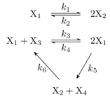
Figure 1: Example network (N1).

According to mass-action kinetics, the network (N1) gives rise to the following system of differential equations on the positive orthant $\mathbb{R}_{>0}^{4}$:

$$\frac{dx_{1}}{dt} =-k_{1}x_{1}+k_{2}x_{2}^{2}+k_{3}x_{1}x_{3}-k_{4}x_{1}^{2}-2k_{5}x_{1}^{2}+k_{6}x_{2}x_{4}$$

$$\frac{dx_{2}}{dt} =2k_{1}x_{1}-2k_{2}x_{2}^{2}+k_{5}x_{1}^{2}-k_{6}x_{2}x_{4}$$ (1)

$$\frac{dx_{3}}{dt} =-k_{3}x_{1}x_{3}+k_{4}x_{1}^{2}+k_{6}x_{2}x_{4}$$

$$\frac{dx_{4}}{dt} =k_{5}x_{1}^{2}-k_{6}x_{2}x_{4},$$

where $x_{i}=[\chemfig{X_{i}}]$ is the concentration of species $\chemfig{X_{i}}$.

At any given time, the concentration vector ${\boldsymbol{x}}(t)=(x_{1}(t),x_{2}(t),\dots,x_{n}(t))^{T}$ is a point in $\mathbb{R}_{>0}^{n}$. Tracing the path over time gives a trajectory in the state space $\mathbb{R}_{>0}^{n}$. For example, Figure 2 shows several trajectories of three mass-action systems. For this reason, any concentration vector ${\boldsymbol{x}}=(x_{1},x_{2},\dots,x_{n})^{T}$ is also called a state of the system, and we will refer to it as such.

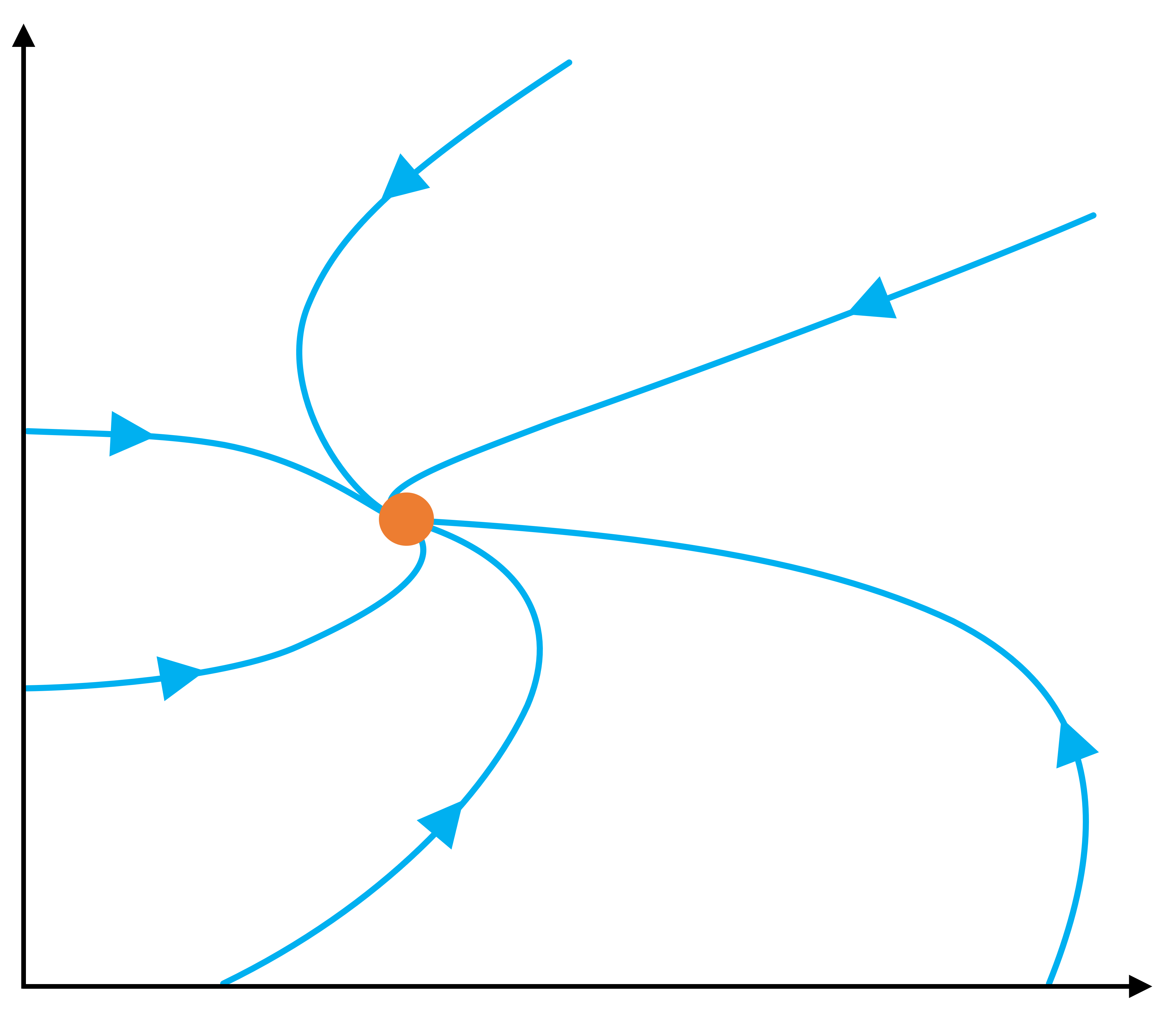
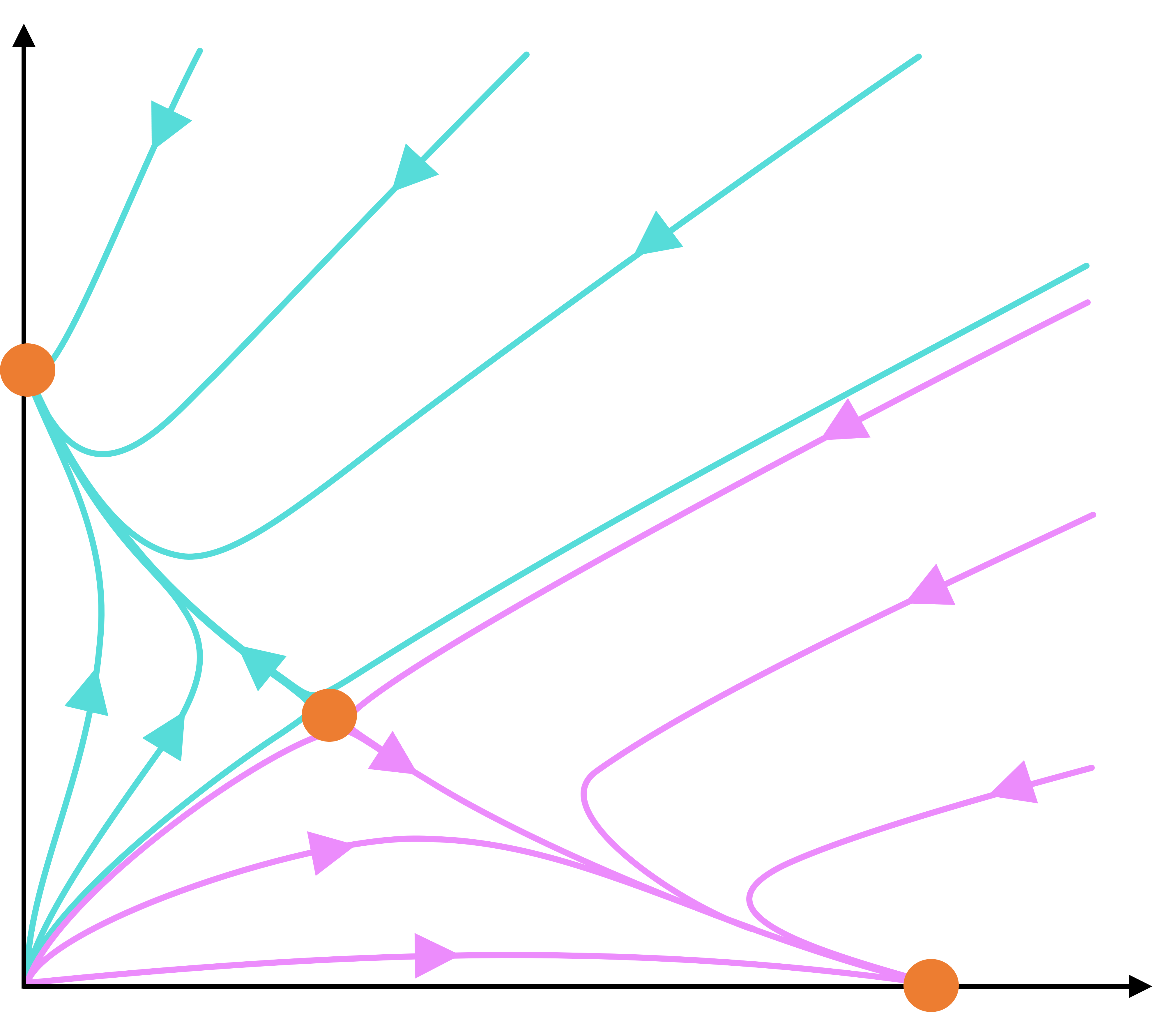
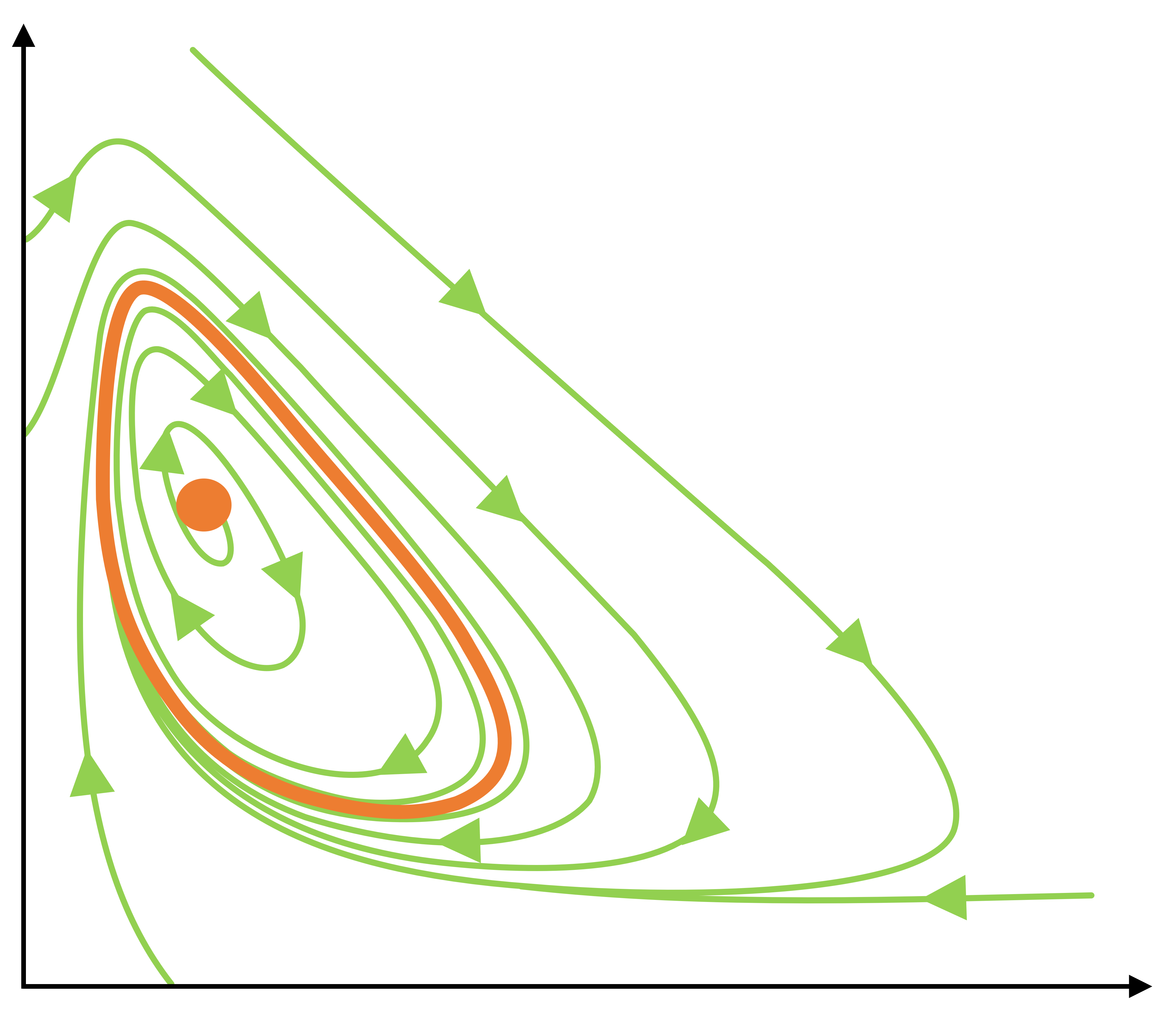
Figure 2: Phase portraits showing possible behaviors of mass-action systems: (a) uniqueness and stability of steady state, (b) bistability, and (c) oscillation. The mass-action systems, with the rate constants labeled on the reaction edges, are (a)   $\varnothing\xrightarrow{0.7}\rm{X}_{1}\xrightarrow{\,1\,}\rm{X}_{1}+\rm{X}_{2}\xrightarrow{\,1\,}\varnothing$,   (b)   $\rm{X}_{1}+\rm{X}_{2}\xrightarrow{\,1\,}\rm{X}_{1}\xrightleftharpoons[\,1\,]{3}2\rm{X}_{1}$ and $\rm{X}_{1}+\rm{X}_{2}\xrightarrow{\,2\,}\rm{X}_{2}\xrightleftharpoons[\,1\,]{2}2\rm{X}_{2}$,   (c)   a version of the Selkov model, or “Brusselator”, whose network (N2) is shown in Figure 3 and rate constants given in Remark LABEL:rmk:oscillation.

In vector-based form, this dynamical system can also be written as

$$\!\!\!\!\!\!\!\!\!\!\!\!\!\!\!\!\!\!\!\frac{d}{dt}\!\!\begin{pmatrix}x_{1}\\ x_{2}\\ x_{3}\\ x_{4}\end{pmatrix}\! =k_{1}x_{1}\!\!\begin{pmatrix}-1\\ 2\\ 0\\ 0\end{pmatrix}\!\!+k_{2}x_{2}^{2}\!\!\begin{pmatrix}1\\ -2\\ 0\\ 0\end{pmatrix}\!\!+k_{3}x_{1}x_{3}\!\!\begin{pmatrix}1\\ 0\\ -1\\ 0\end{pmatrix}\!\!$$

$$\qquad+k_{4}x_{1}^{2}\!\!\begin{pmatrix}-1\\ 0\\ 1\\ 0\end{pmatrix}\!\!+k_{5}x_{1}^{2}\!\!\begin{pmatrix}-2\\ 1\\ 0\\ 1\end{pmatrix}\!\!+k_{6}x_{2}x_{4}\!\!\begin{pmatrix}1\\ -1\\ 1\\ -1\end{pmatrix}.$$ (2)

In order to write down a general mathematical formula for mass-action systems we need to introduce more definitions and notation.

The objects that are the source or the target of a reaction are called complexes. For example, the complexes in the network (N1) are $\rm{X}_{1}$, $2\rm{X}_{2}$, $\rm{X}_{1}+\rm{X}_{3}$, $2\rm{X}_{1}$, and $\rm{X}_{2}+\rm{X}_{4}$. Their complex vectors are the vectors $\displaystyle\begin{pmatrix}1\\ 0\\ 0\\ 0\end{pmatrix}$, $\displaystyle\begin{pmatrix}0\\ 2\\ 0\\ 0\end{pmatrix}$, $\displaystyle\begin{pmatrix}1\\ 0\\ 1\\ 0\end{pmatrix}$, $\displaystyle\begin{pmatrix}2\\ 0\\ 0\\ 0\end{pmatrix}$, and $\displaystyle\begin{pmatrix}0\\ 1\\ 0\\ 1\end{pmatrix}$, respectively.

Let us introduce the notation

$${\boldsymbol{x}}^{\boldsymbol{y}}=x_{1}^{y_{1}}x_{2}^{y_{2}}\cdots x_{n}^{y_{n}}$$ (3)

for any two vectors ${\boldsymbol{x}}=(x_{1},x_{2},\dots,x_{n})^{T}\in\mathbb{R}^{n}_{>0}$ and ${\boldsymbol{y}}=(y_{1},y_{2},\dots,y_{n})^{T}\in\mathbb{R}^{n}_{\geq 0}$. Then the monomials $x_{1}$, $x_{2}^{2}$, $x_{1}x_{3},\dots$, in the reaction rate functions in (1) can be represented as ${\boldsymbol{x}}^{\boldsymbol{y}}$, where ${\boldsymbol{x}}$ is the vector of species concentrations and ${\boldsymbol{y}}$ is the complex vector of the source of the corresponding reaction. For example, $\rm{X}_{1}+\rm{X}_{3}$ is the source of the reaction $\rm{X}_{1}+\rm{X}_{3}\to\rm{X}_{4}$, its complex vector is $\displaystyle\begin{pmatrix}1\\ 0\\ 1\\ 0\end{pmatrix}$, and the corresponding reaction rate function in (1) is $k_{3}x_{1}x_{3}$.

The vectors in (1) are called reaction vectors, and they are the differences between the complex vectors of the target and source of each reaction; a reaction vector records the stoichiometry of the reaction. For example, the reaction vector corresponding to $\rm{X}_{1}+\rm{X}_{3}\to\rm{X}_{4}$ is $\displaystyle\begin{pmatrix}-1\\ 0\\ -1\\ 1\end{pmatrix}=\begin{pmatrix}0\\ 0\\ 0\\ 1\end{pmatrix}-\begin{pmatrix}1\\ 0\\ 1\\ 0\end{pmatrix}$.

There is a naturally defined oriented graph underlying a reaction network, namely the graph where the vertices are complexes, and the edges are reactions. Therefore, a chemical reaction network can be regarded as a Euclidean embedded graph $G=(V,E)$, where $V\subset\mathbb{R}^{n}_{\geq 0}$ is the set of vertices of the graph, and $E\subset V\times V$ is the set of oriented edges of $G$.

For example, (N2) depicted in Figure 3 is the network for a version of the Selkov model for glycolysis.

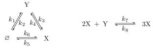
Figure 3: Example network (N2), a version of the Selkov model for glycolysis. It can also be regarded as a version of the “Brusselator”.

Its Euclidean embedded graph $G$ in $\mathbb{R}_{\geq 0}^{2}$ is shown in Figure 4.

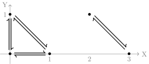
Figure 4: The Euclidean embedded graph $G$ of the network (N2) as shown in Figure 3.

Given a reaction network with its Euclidean embedded graph $G$, and given a vector of reaction rate constants ${\boldsymbol{k}}$, we can use the notation (3) to write the mass-action system generated by $(G,{\boldsymbol{k}})$ as shown in (4)

$$\frac{d{\boldsymbol{x}}}{dt} =\sum_{{\boldsymbol{y}}\to{\boldsymbol{y}}^{\prime}\in G}k_{{\boldsymbol{y}}\to{\boldsymbol{y}}^{\prime}}{\boldsymbol{x}}^{{\boldsymbol{y}}}\left({\boldsymbol{y}}^{\prime}-{\boldsymbol{y}}\right).$$ (4)

The stoichiometric subspace $S$ of a reaction network $G$ is the vector space spanned by its reaction vectors:

$$S=\operatorname{span}_{\mathbb{R}}\{{\boldsymbol{y}}^{\prime}-{\boldsymbol{y}}:{\boldsymbol{y}}\to{\boldsymbol{y}}^{\prime}\in G\}.$$ (5)

The stoichiometric compatibility class of ${\boldsymbol{x}}_{0}\in\mathbb{R}_{>0}^{n}$ is the set $({\boldsymbol{x}}_{0}+S)_{>0}=({\boldsymbol{x}}_{0}+S)\cap\mathbb{R}_{>0}^{n}$, i.e., the intersection between the affine set ${\boldsymbol{x}}_{0}+S$ and the positive orthant. Note that the solution ${\boldsymbol{x}}(t)$ of the mass-action system with initial condition ${\boldsymbol{x}}_{0}$ is confined to $({\boldsymbol{x}}_{0}+S)_{>0}$ for all future time, i.e., each stoichiometric compatibility class is a forward invariant set [Feinberg_1979].

We say that a network or a graph $G$ is reversible if ${\boldsymbol{y}}^{\prime}\to{\boldsymbol{y}}$ is a reaction whenever ${\boldsymbol{y}}\to{\boldsymbol{y}}^{\prime}$ is a reaction. We say that $G$ is weakly reversible if every reaction is part of an oriented cycle, i.e., each connected component of the graph $G$ is strongly connected. The network (N1) is weakly reversible, while (N2) is reversible. When the underlying graph $G$ is weakly reversible, we will see that the solutions of the mass-action system are known (or conjectured) to have many important properties, such as existence of positive steady states for all parameter values, persistence, permanence, and if the network satisfies some additional assumptions, also global stability [CNP, TDS, Craciun_GAC, Horn_Jackson, gunawardena, Feinberg_1979].

For example, in the next section we will see that the mass-action systems generated by network (N1) and any values of rate constants are globally stable, i.e., there exists a globally attracting steady state within each stoichiometric compatibility class.

2 Results Inspired by Thermodynamic Principles

The idea of relating chemical kinetics and thermodynamics has a very long history, starting with Wegscheider [Wegscheider_1902], and continuing with Lewis [Lewis_1925], Onsager [Onsager_1931], Wei and Prater [WeiPrater_1962], Aris [Aris_1965], Shear [Shear_1967], Higgins [Higgins_1968], and many others. For example, the notion of “detailed-balanced systems” was studied in depth, and this notion has a strong connection to the thermodynamical properties of microscopic reversibility which goes back to Boltzmann [Boltzmann_1887, Boltzmann_1896, Gorban_Karlin_2005].

2.1 Detailed-Balanced and Complex-Balanced Systems

In 1972 Horn and Jackson [Horn_Jackson] have identified the class of “complex-balanced systems” as a generalization of detailed-balanced systems. While complex-balanced systems are not necessarily thermodynamically closed systems, Horn and Jackson were interested in systems that behave as though the laws of thermodynamics for closed systems are obeyed. In particular, according to the Horn-Jackson theorem below, a complex-balanced system has a unique steady state within each stoichiometric compatibility class, and it is locally stable within it [Horn_Jackson].

Of all the positive steady states, we call attention to two kinds that are especially important. These are characterized by the fluxes at a state ${\boldsymbol{x}}_{0}$, i.e., the values $k_{{\boldsymbol{y}}\to{\boldsymbol{y}}^{\prime}}{\boldsymbol{x}}_{0}^{{\boldsymbol{y}}}$ of the reaction rate functions evaluated at ${\boldsymbol{x}}_{0}$.

Definition 2.1.

A state ${\boldsymbol{x}}_{0}$ of a mass-action system is a detailed-balanced steady state if the network is reversible, and every forward flux is balanced by the backward flux at that state, i.e., for every reaction pair ${\boldsymbol{y}}\rightleftharpoons{\boldsymbol{y}}^{\prime}$, we have

$$k_{{\boldsymbol{y}}\to{\boldsymbol{y}}^{\prime}}{\boldsymbol{x}}_{0}^{{\boldsymbol{y}}}=k_{{\boldsymbol{y}}^{\prime}\to{\boldsymbol{y}}}{\boldsymbol{x}}_{0}^{{\boldsymbol{y}}^{\prime}}.$$ (6)

In particular, if a network is not reversible, then it cannot admit a detailed-balanced steady state.

A state ${\boldsymbol{x}}_{0}$ of a mass-action system is a complex-balanced steady state if at each vertex of the corresponding Euclidean embedded graph $G$, the fluxes flowing into the vertex balance the fluxes flowing out of the vertex at that state ${\boldsymbol{x}}_{0}$, i.e., for every complex ${\boldsymbol{y}}$ we have

$$\sum_{{\boldsymbol{y}}\to{\boldsymbol{y}}^{\prime}\in G}k_{{\boldsymbol{y}}\to{\boldsymbol{y}}^{\prime}}{\boldsymbol{x}}_{0}^{{\boldsymbol{y}}}\ =\sum_{{\boldsymbol{y}}^{\prime}\to{\boldsymbol{y}}\in G}k_{{\boldsymbol{y}}^{\prime}\to{\boldsymbol{y}}}{\boldsymbol{x}}_{0}^{{\boldsymbol{y}}^{\prime}}$$ (7)

In particular, it can be shown that if the network is not weakly reversible, then it cannot admit a complex-balanced steady state.

At a detailed-balanced steady state ${\boldsymbol{x}}_{0}$, the fluxes across pairs of reversible reactions are balanced; hence ${\boldsymbol{x}}_{0}$ is also called an edge-balanced steady state. At a complex-balanced steady state ${\boldsymbol{x}}_{0}$, the net flux through any vertex is zero; hence ${\boldsymbol{x}}_{0}$ is also called a vertex-balanced steady state.

Definition 2.2.

A detailed-balanced system is a mass-action system $(G,{\boldsymbol{k}})$ that has at least one detailed-balanced steady state. A complex-balanced system is a mass-action system $(G,{\boldsymbol{k}})$ that has at least one complex-balanced steady state.

It is not difficult to check that if the state ${\boldsymbol{x}}_{0}$ is detailed-balanced, then it is complex-balanced, i.e., complex balance is a generalization of detailed balance. Complex-balanced systems enjoy many properties of detailed-balanced systems; the Horn-Jackson theorem is the first such result.

Theorem 2.3 (Horn-Jackson theorem [Horn_Jackson]).

Consider a reaction network $G$ and a vector of reaction rate constants ${\boldsymbol{k}}$. Assume that the mass-action system generated by $(G,{\boldsymbol{k}})$ has a complex-balanced steady state ${\boldsymbol{x}}^{*}$; in other words, $(G,{\boldsymbol{k}})$ is a complex-balanced system. Then all of the following properties hold:

1. All positive steady states are complex-balanced, and there is exactly one steady state within every stoichiometric compatibility class.

2. The set of complex-balanced steady states $Z_{{\boldsymbol{k}}}$ satisfies the equation $\ln Z_{{\boldsymbol{k}}}=\ln{\boldsymbol{x}}^{*}+S^{\perp}$, where $S$ is the stoichiometric subspace of $G$.

3. The function

   $$L({\boldsymbol{x}})=\sum_{j=1}^{n}x_{i}(\ln x_{i}-\ln x_{i}^{*}-1).$$ (8)

   is a strictly convex Lyapunov function of this system, defined on $\mathbb{R}_{>0}^{n}$ and with global minimum at ${\boldsymbol{x}}={\boldsymbol{x}}^{*}$.

4. Every positive steady state is locally asymptotically stable within its stoichiometric compatibility class.

Remark 2.4.

The original paper of Horn and Jackson [Horn_Jackson] claimed that each complex-balanced steady state is a global attractor within its stoichiometric compatibility class. Later, Horn [Horn_1974] realized that this claim does not follow from the existence of the Lyapunov function above, and formulated it as a conjecture, later known as the “global attractor conjecture” (see Section LABEL:sec:GAC).