Superintegrable metrics on surfaces admitting integrals of degrees 1 and 4

Pavel Novichkov

National Research University Higher School of Economics,
Faculty of Mathematics, Moscow, Russia

  Abstract
We study Riemannian metrics on surfaces whose geodesic flows are superintegrable with one integral linear in momenta and one integral quartic in momenta. The main results of the work are local description of such metrics in terms of ordinary differential equations, integration of the equations, and description of the corresponding Poisson algebra of integrals of motion. We also give examples of such metrics that can be extended to the sphere $S^{2}$, and study the group of symmetries of the problem.  

1 Introduction

Let $\mathcal{M}$ be a smooth $n$-dimensional Riemannian manifold with metric $g=(g_{ij})$. Let $g^{*}=(g^{ij})$ be a dual metric tensor which defines a metric on the cotangent bundle $T^{*}\mathcal{M}$. It is well known that the geodesic flow on $\mathcal{M}$ can be described as the Hamiltonian flow on $T^{*}\mathcal{M}$ with the Hamiltonian $H_{g}:=\frac{1}{2}g^{*}$. The corresponding mechanical system on $T^{*}\mathcal{M}$ is called free. $H_{g}$ is called its kinetic energy. Recall also that a Hamiltonian mechanical system with Hamiltonian $H$ defined on a symplectic manifold $(X,\omega)$ is called (Liouville) integrable if it allows $n$ functionally independent integrals $H=X_{1},\,X_{2},\ldots,X_{n}$ in involution. An integrable system is called superintegrable if it allows further functionally independent integrals $Y_{1},\,Y_{2},\ldots,Y_{k},\,1\leq k\leq n-1$ (not necessarily in involution with each other nor with $X_{i}$). If a free Hamiltonian system is superintegrable then the corresponding metric $g$ is also called superintegrable.

Classical examples of integrable systems include Kepler-Coulomb problem, 2 and 3-dimensional isotropic harmonic oscillator, and hydrogen atom. All of them turn out to be superintegrable. For instance, Kepler-Coulomb problem has 7 integrals of motion (energy, 3 components of angular momentum vector and 3 components of Laplace-Runge-Lenz vector). These integrals are related by 2 scalar equations, hence there are 5 functionally independent integrals.

Superintegrable systems are of great interest for modern mathematics and mathematical physics due to several special properties they have:

• if a superintegrable system has $k$ extra integrals, then its trajectories lie on $(n-k)$-dimensional submanifolds;

• in particular, when $k=n-1$ (so called maximal superintegrability) all trajectories lie on 1-dimensional submanifolds, hence all finite trajectories are closed;

• integrals of motion generate a nontrivial Poisson algebra;

• extra integrals correspond to hidden symmetries;

• in quantum physics, superintegrability leads to accidental degeneracy of energy levels

etc. [1].

One natural question that arises here is how to find and describe all superintegrable systems in simple cases. The simplest nontrivial possibility in terms of dimension is $n=2$. A 2-dimensional superintegrable system has 2 extra integrals besides energy. Obviously, such a system is maximally superintegrable. Let us also restrict ourselves to considering free superintegrable systems (i.e., searching for superintegrable metrics). Finally, let us assume that integrals of motion are polynomial in momenta. This assumption is motivated by real-world physical examples of such systems, and by the Whittaker theorem (if a system allows an integral analytical in momenta then it also allows an integral polynomial in momenta [2]).

One can easily show that each homogeneous component of a polynomial integral is an integral by itself, therefore it is sufficient to consider homogeneous integrals of degrees $l$ and $m$. Let us call this case “$l+m$”.

In the case “$1+1$” each superintegrable metric has constant curvature. Cases “$1+2$” and “$2+2$” were described locally in the classical work by Koenigs [3]. Finally, local description of “$1+3$” metrics was obtained in [4, 5].

The aim of this work is to describe superintegrable metrics in the next case “$1+4$”. We develop methods and ideas used in [4] to solve the case “$1+3$”. In Chapter 2, we formulate and prove the theorem which gives local description of “$1+4$” superintegrable metrics in the neighborhood of almost every point. In Chapter 3, we study symmetries of such systems and obtain algebraic forms of the equations describing the metrics. It allows us to construct examples of the metrics that can be extended to the sphere.

The author is grateful to his advisor Vsevolod Shevchishin for his continuous support and many useful discussions.

2 Local description of 2-dimensional superintegrable metrics admitting integrals of degrees 1 and 4

2.1 Main result

Theorem 2.1.

Let $\mathcal{M}^{2}$ be a smooth 2-dimensional manifold equipped with a Riemannian metric $g=(g_{ij})$. Let $H=\frac{1}{2}g^{ij}p_{i}p_{j}$ be the corresponding Hamiltonian.

Suppose the geodesic flow of $g$ admits integrals $L$ and $F$ of degrees 1 and 4 such that $L,\,F$ and $H$ are functionally independent. Then in the neighborhood of almost every point $X\in\mathcal{M}^{2}$ (such that $L|_{T^{*}_{X}\mathcal{M}^{2}}\not\equiv 0$) there exist local coordinates $(x,y)$ such that the metric has the form $g=\frac{1}{h_{x}^{2}}(dx^{2}+dy^{2})$ where $h_{x}\equiv\dfrac{dh}{dx}$ and $h(x)$ is a real function that satisfies one of the following systems of equations:

$$\begin{cases}\begin{gathered}2\left(A_{0}h-A_{1}\right)\left(A_{3}\cos(\mu x)+\frac{A_{4}}{\mu}\sin(\mu x)\right)h_{x}^{3}\\ +\left[\left(\mu\left(A_{0}h-2A_{1}\right)h+2\,\frac{A_{2}}{\mu}\right)\left(A_{3}\sin(\mu x)-\frac{A_{4}}{\mu}\cos(\mu x)\right)+A_{5}\right]h_{x}^{2}\\ -\left(A_{3}\cos(\mu x)+\frac{A_{4}}{\mu}\sin(\mu x)\right)^{2}=0,\end{gathered}\\ \begin{gathered}\left(A_{0}h-A_{1}\right)^{2}h_{x}^{3}\,+\left[\frac{\mu}{2}\left(A_{0}h-2A_{1}\right)h\left(\frac{\mu}{2}\left(A_{0}h-2A_{1}\right)h+2\,\frac{A_{2}}{\mu}\right)\right.\\ \left.+\,2\,\frac{A_{0}}{\mu}\left(A_{3}\sin(\mu x)-\frac{A_{4}}{\mu}\cos(\mu x)\right)+\frac{A_{6}}{4\mu^{2}}\right]h_{x}\\ -\,2\left(A_{0}h-A_{1}\right)\left(A_{3}\cos(\mu x)+\frac{A_{4}}{\mu}\sin(\mu x)\right)=0,\end{gathered}\end{cases}$$ (2.1.1a)

$$\begin{cases}\begin{gathered}2\left(A_{0}h-A_{1}\right)\left(A_{3}\cosh(\mu x)+\frac{A_{4}}{\mu}\sinh(\mu x)\right)h_{x}^{3}\\ -\left[\left(\mu\left(A_{0}h-2A_{1}\right)h-2\,\frac{A_{2}}{\mu}\right)\left(A_{3}\sinh(\mu x)+\frac{A_{4}}{\mu}\cosh(\mu x)\right)-A_{5}\right]h_{x}^{2}\\ -\left(A_{3}\cosh(\mu x)+\frac{A_{4}}{\mu}\sinh(\mu x)\right)^{2}=0,\end{gathered}\\ \begin{gathered}\left(A_{0}h-A_{1}\right)^{2}h_{x}^{3}\,-\left[\frac{\mu}{2}\left(A_{0}h-2A_{1}\right)h\left(\frac{\mu}{2}\left(A_{0}h-2A_{1}\right)h-2\,\frac{A_{2}}{\mu}\right)\right.\\ \left.-\,2\,\frac{A_{0}}{\mu}\left(A_{3}\sinh(\mu x)+\frac{A_{4}}{\mu}\cosh(\mu x)\right)+\frac{A_{6}}{4\mu^{2}}\right]h_{x}\\ -\,2\left(A_{0}h-A_{1}\right)\left(A_{3}\cosh(\mu x)+\frac{A_{4}}{\mu}\sinh(\mu x)\right)=0,\end{gathered}\end{cases}$$ (2.1.1b)

$$\begin{cases}\begin{gathered}2\left(A_{0}h-A_{1}\right)\left(A_{3}+A_{4}x\right)h_{x}^{3}+\left(A_{4}h\left(2A_{1}-A_{0}h\right)\right.\\ \left.+A_{2}x\left(2A_{3}+A_{4}x\right)+A_{5}\right)h_{x}^{2}-\left(A_{3}+A_{4}x\right)^{2}=0,\end{gathered}\\ \begin{gathered}\left(A_{0}h-A_{1}\right)^{2}h_{x}^{3}+\left(\left(A_{0}h-2A_{1}\right)A_{2}h+A_{0}x\left(2A_{3}+A_{4}x\right)+A_{6}\right)h_{x}\\ -\,2\left(A_{0}h-A_{1}\right)\left(A_{3}+A_{4}x\right)=0\end{gathered}\end{cases}$$ (2.1.1c)

Here $\mu>0,\,A_{0},\ldots,A_{6}$ are arbitrary real constants.

Further, the linear integral $L$ is given by $L=p_{y}$.

Besides, in the case (a) the metric admits 2-parametric family of quartic integrals of the form

$$F=C_{+}F_{+}+C_{-}F_{-},$$ (2.1.2)

where

$$\begin{gathered}F_{+}=e^{\mu y}\sum_{k=0}^{4}a_{k}(x)p_{x}^{4-k}p_{y}^{k},\\ F_{-}=e^{-\mu y}\sum_{k=0}^{4}(-1)^{k}a_{k}(x)p_{x}^{4-k}p_{y}^{k}.\end{gathered}$$ (2.1.3)

Here $C_{+},\,C_{-}$ are arbitrary real constants, and functions $a_{k}(x)$ are given by

$$a_{0}(x)=\frac{A_{0}}{\mu}h_{x}^{4},$$ (2.1.4)

$$a_{1}(x)=(A_{1}-A_{0}h)h_{x}^{3},$$

$$a_{2}(x)=\left(\frac{1}{2}\mu A_{0}h^{2}+\frac{2A_{0}}{\mu}h_{x}^{2}-\mu A_{1}h+\frac{A_{2}}{\mu}\right)h_{x}^{2},$$

$$a_{3}(x)=(A_{1}-A_{0}h)h_{x}^{3}-\left(A_{3}\cos(\mu x)+\frac{A_{4}}{\mu}\sin(\mu x)\right),$$

$$\begin{gathered}a_{4}(x)=\left(\frac{\mu}{2}(A_{0}h-2A_{1})h+\frac{A_{0}}{\mu}h_{x}^{2}+\frac{A_{2}}{\mu}\right)h_{x}^{2}+\left(A_{3}\sin(\mu x)-\frac{A_{4}}{\mu}\cos(\mu x)\right).\end{gathered}$$

Next, in the case (b) the metric admits 2-parametric family of quartic integrals of the form

$$F= \,\,C_{e}\cos(\mu y+\phi_{0})\,\left(a_{0}(x)\,p_{x}^{4}+a_{2}(x)\,p_{x}^{2}p_{y}^{2}+a_{4}(x)\,p_{y}^{4}\right)$$ (2.1.5)

$$+ \,\,C_{e}\sin(\mu y+\phi_{0})\,\left(a_{1}(x)\,p_{x}^{3}p_{y}+a_{3}(x)\,p_{x}p_{y}^{3}\right),$$

where $C_{e},\,\phi_{0}$ are arbitrary real constants, and functions $a_{k}(x)$ are given by

$$a_{0}(x)=-\frac{A_{0}}{\mu}h_{x}^{4},$$ (2.1.6)

$$a_{1}(x)=(A_{1}-A_{0}h)h_{x}^{3},$$

$$a_{2}(x)=\left(\frac{1}{2}\mu A_{0}h^{2}-\frac{2A_{0}}{\mu}h_{x}^{2}-\mu A_{1}h-\frac{A_{2}}{\mu}\right)h_{x}^{2},$$

$$a_{3}(x)=(A_{1}-A_{0}h)h_{x}^{3}-\left(A_{3}\cosh(\mu x)+\frac{A_{4}}{\mu}\sinh(\mu x)\right),$$

$$\begin{gathered}a_{4}(x)=\left(\frac{\mu}{2}(A_{0}h-2A_{1})h-\frac{A_{0}}{\mu}h_{x}^{2}-\frac{A_{2}}{\mu}\right)h_{x}^{2}+\left(A_{3}\sinh(\mu x)+\frac{A_{4}}{\mu}\cosh(\mu x)\right).\end{gathered}$$

Finally, in the case (c) the metric admits a quartic integral of the form

$$\begin{gathered}F=y\left(a_{0}(x)p_{x}^{4}+a_{2}(x)p_{x}^{2}p_{y}^{2}+a_{4}(x)p_{y}^{4}\right)+a_{1}(x)p_{x}^{3}p_{y}+a_{3}(x)p_{x}p_{y}^{3}\,,\end{gathered}$$ (2.1.7)

where functions $a_{k}(x)$ are given by

$$a_{0}(x)=A_{0}h_{x}^{4},$$ (2.1.8)

$$a_{1}(x)=(A_{1}-A_{0}h)h_{x}^{3},$$

$$a_{2}(x)=(2A_{0}h_{x}^{2}+A_{2})h_{x}^{2},$$

$$a_{3}(x)=(A_{1}-A_{0}h)h_{x}^{3}-(A_{3}+A_{4}x),$$

$$a_{4}(x)=-A_{4}+A_{2}h_{x}^{2}+A_{0}h_{x}^{4}.$$

Remark 2.1.

Actually, any equation in each pair (2.1.1) is sufficient to describe the function $h(x)$. However, second equation allows to eliminate $h_{x}$ (see 3.2 for details), therefore the system of two equations is an implicit way to integrate each of them. The constants $A_{5}$ and $A_{6}$ play an important role here: in fact, the choice of $A_{6}$ for the second equation is equivalent to the choice of initial conditions for the first equation, and vice versa.

2.2 Reduction to a 3rd order ODE

Since the metric $g$ allows the linear integral $L$ it follows that in the neighborhood of every point $X\in\mathcal{M}^{2}$ such that $L|_{T^{*}_{X}\mathcal{M}^{2}}\not\equiv 0$ there exist local coordinates $(x,y)$ such that the metric and the linear integral have the form

$$g=\lambda(x)\left(dx^{2}+dy^{2}\right),\quad L=p_{y},$$ (2.2.1)

where $\lambda(x)$ is a real function [6]. It means that superintegrability condition can be expressed as a condition on the function $\lambda(x).$ Namely, quartic integral has the following form in our coordinates:

$$F=\sum_{k=0}^{4}\tilde{a}_{k}(x,y)p_{x}^{4-k}p_{y}^{k},$$ (2.2.2)

where $\tilde{a}_{k}(x,y)$ are some unknown functions. The condition $\{F,H\}=0$ is equivalent to a system of partial differential equations on the functions $\tilde{a}_{k}(x,y)$ and $\lambda(x).$ Solving this system, we can obtain superintegrability condition as an equation on $\lambda(x)$, and an explicit formula for the quartic integral.

However this system of equations is extremely complicated, therefore it is useful to reduce our problem to a simpler system of ordinary differential equations. To do that, we need to eliminate one of the variables.

Following [4], let us consider a linear operator

$$\mathcal{L}\colon F\mapsto\{L,F\}$$

acting on the space $\mathscr{J}_{4}$ of complex quartic integrals in the neighborhood of $X$ (complexification is needed to guarantee that $\mathcal{L}$ has eigenvalues). $\mathcal{L}$ is well-defined: first, Poisson bracket of two integrals is an integral due to the Jacobi identity; secondly, $\deg\{L,F\}=\deg L+\deg F-1=\deg F.$ Note also that $\mathscr{J}_{4}$ is a finite-dimensional space. Namely, $\dim\mathscr{J}_{4}\leq 15$ [7].

It is readily seen that $L^{4},\,L^{2}H$ and $H^{2}$ are eigenvectors of $\mathcal{L}$ with an eigenvalue of $0$. Two cases are possible:

1. There exists a nonzero eigenvalue of $\mathcal{L}$: $\mu\neq 0,\mu\in\mathbb{C}$.

2. The spectrum of $\mathcal{L}$ is $\{0\}$.

Let us consider the basic case $\mu\neq 0\,$; the case $\mu=0$ will be considered later in Chapter 2.6.

Assume there exists a complex quartic integral

$$F=\sum_{k=0}^{4}\tilde{a}_{k}(x,y)\,p_{x}^{4-k}p_{y}^{k}$$ (2.2.3)

(this time functions $\tilde{a}_{k}(x,y)$ are complex-valued) such that $\{L,F\}=\partial_{y}F=\mu F,$ i.e. $\partial_{y}\tilde{a}_{k}(x,y)=\mu\,\tilde{a}_{k}(x,y),\,k=0,\ldots,4.$ It follows that $\tilde{a}_{k}(x,y)=e^{\mu y}\,a_{k}(x)$ for some functions $a_{k}(x).$ Thus the integral $F$ has the form

$$F=e^{\mu y}\sum_{k=0}^{4}a_{k}(x)\,p_{x}^{4-k}p_{y}^{k}.$$ (2.2.4)

For convenience in further calculations, let us rewrite the metric as

$$g=\frac{1}{h_{x}^{2}}(dx^{2}+dy^{2})$$ (2.2.5)

for some function $h(x).$ Then $H=\dfrac{h_{x}^{2}}{2}(p_{x}^{2}+p_{y}^{2})$, and the condition $\{F,H\}=0$ reads

$$e^{\mu y}h_{x}\,\left(a_{0}^{\prime}(x)h_{x}-4a_{0}(x)h_{xx}\right) \,\,p_{x}^{5}$$ (2.2.6)

$$+\,e^{\mu y}\,h_{x}\left(\mu a_{0}(x)h_{x}+a_{1}^{\prime}(x)h_{x}-3a_{1}(x)h_{xx}\right) \,\,p_{x}^{4}p_{y}$$

$$+\,e^{\mu y}\,h_{x}\left(\mu a_{1}(x)h_{x}+a_{2}^{\prime}(x)h_{x}-4a_{0}(x)h_{xx}-2a_{2}(x)h_{xx}\right) \,\,p_{x}^{3}p_{y}^{2}$$

$$+\,e^{\mu y}\,h_{x}\left(\mu a_{2}(x)h_{x}+a_{3}^{\prime}(x)h_{x}-3a_{1}(x)h_{xx}-a_{3}(x)h_{xx}\right) \,\,p_{x}^{2}p_{y}^{3}$$

$$+\,e^{\mu y}\,h_{x}\left(\mu a_{3}(x)h_{x}+a_{4}^{\prime}(x)h_{x}-2a_{2}(x)h_{xx}\right) \,\,p_{x}p_{y}^{4}$$

$$+\,e^{\mu y}\,h_{x}\left(\mu a_{4}(x)h_{x}-a_{3}(x)h_{xx}\right) \,\,p_{y}^{5}=0.$$

Since the monomials $p_{x}^{5-k}p_{y}^{k}$ form a basis in the space of homogeneous polynomials of degree 5, every term in (2.2.6) should vanish. This gives us the following system of 6 equations on the functions $h(x),a_{0}(x),\ldots,a_{4}(x)$:

$$a_{0}^{\prime}(x)h_{x}-4a_{0}(x)h_{xx} =0,$$ (2.2.7a)

$$\mu a_{0}(x)h_{x}+a_{1}^{\prime}(x)h_{x}-3a_{1}(x)h_{xx} =0,$$ (2.2.7b)

$$\mu a_{1}(x)h_{x}+a_{2}^{\prime}(x)h_{x}-4a_{0}(x)h_{xx}-2a_{2}(x)h_{xx} =0,$$ (2.2.7c)

$$\mu a_{2}(x)h_{x}+a_{3}^{\prime}(x)h_{x}-3a_{1}(x)h_{xx}-a_{3}(x)h_{xx} =0,$$ (2.2.7d)

$$\mu a_{3}(x)h_{x}+a_{4}^{\prime}(x)h_{x}-2a_{2}(x)h_{xx} =0,$$ (2.2.7e)

$$\mu a_{4}(x)h_{x}-a_{3}(x)h_{xx} =0.$$ (2.2.7f)

Subsequently solving 2.2.7a, 2.2.7b and 2.2.7c, we get

$$a_{0}(x) =\frac{A_{0}}{\mu}h_{x}^{4},$$ (2.2.8a)

$$a_{1}(x) =(A_{1}-A_{0}h)h_{x}^{3},$$ (2.2.8b)

$$a_{2}(x) =\left(\frac{1}{2}\mu A_{0}h^{2}+\frac{2A_{0}}{\mu}h_{x}^{2}-\mu A_{1}h+\frac{A_{2}}{\mu}\right)h_{x}^{2},$$ (2.2.8c)

where $A_{0},A_{1}$ and $A_{2}$ are complex constants of integration. Also, we can eliminate $a_{4}(x)$ using 2.2.7f:

$$a_{4}(x)=a_{3}(x)\cfrac{h_{xx}}{\mu\,h_{x}}.$$ (2.2.9)

Unfortunately, there is no explicit way to eliminate $a_{3}(x)$ after substituting these expressions for $a_{0}(x),\,a_{1}(x),\,a_{2}(x)$ and $a_{4}(x)$ into the remaining equations 2.2.7d and 2.2.7e. However we can use the following trick. Consider formal complex local coordinates

$$z=x+\mathrm{\bf{i}}\,y,\,\bar{z}=x-\mathrm{\bf{i}}\,y$$ (2.2.10)

and the corresponding local momenta

$$p_{z}=\frac{1}{2}\left(p_{x}-\mathrm{\bf{i}}\,p_{y}\right),\,p_{\bar{z}}=\frac{1}{2}\left(p_{x}+\mathrm{\bf{i}}\,p_{y}\right).$$ (2.2.11)

In the new coordinates the integral $F$ reads

$$F=\sum_{k=0}^{4}F_{4-k,k}(z,\bar{z})\,p_{z}^{4-k}p_{\bar{z}}^{k}.$$ (2.2.12)

Proposition 2.1.

The function $F_{4,0}$ is holomorphic.

Proof.

In the new coordinates we have $H=2\,h_{x}^{2}(z,\bar{z})\,p_{z}p_{\bar{z}}$. Poisson bracket $\{F,H\}$ can be expanded as

$$\begin{gathered}\{F,H\}=\left(\partial_{z}F\partial_{p_{z}}H-\partial_{p_{z}}F\partial_{z}H\right)+\left(\partial_{\bar{z}}F\partial_{p_{\bar{z}}}H-\partial_{p_{\bar{z}}}F\partial_{\bar{z}}H\right)=0.\end{gathered}$$

Since the bracket equals zero, the coefficient of $p_{z}^{5}$ should vanish. Clearly, this coefficient comes only from the term $\partial_{\bar{z}}F\partial_{p_{\bar{z}}}H$. It is equal to $\partial_{\bar{z}}F_{4,0}\,p_{z}^{4}\cdot 2\,h_{x}^{2}\,p_{z}$, hence $\partial_{\bar{z}}F_{4,0}=0$. ∎

Calculating $F_{4,0}$ explicitly, we have

$$\begin{gathered}F_{4,0}=e^{\mu y}\bigg{[}\left(\frac{h_{xx}}{\mu h_{x}}-\mathrm{\bf{i}}\,\right)a_{3}(x)-\left(\frac{1}{2}\,\mu A_{0}h^{2}+\frac{A_{0}}{\mu}h_{x}^{2}-\mu A_{1}h+\frac{A_{2}}{\mu}\right)h_{x}^{2}\\ +\,\mathrm{\bf{i}}\,(A_{1}-A_{0}h)h_{x}^{3}\bigg{]}\equiv e^{\mu y}\,G(x).\end{gathered}$$ (2.2.13)

Since $F_{4,0}=e^{\mu y}G(x)=e^{-\mathrm{\bf{i}}\,\mu z}\cdot e^{\mathrm{\bf{i}}\,\mu x}G(x)$ is holomorphic, it follows that $e^{\mathrm{\bf{i}}\,\mu x}G(x)$ has to be constant:

$$e^{\mathrm{\bf{i}}\,\mu x}G(x)=A_{c},\quad G(x)=e^{-\mathrm{\bf{i}}\,\mu x}A_{c}.$$ (2.2.14)

Solving (2.2.13) for $a_{3}(x)$ and taking into account (2.2.14), we obtain

$$\begin{gathered}a_{3}(x)=\frac{1}{\dfrac{h_{xx}}{\mu h_{x}}-\mathrm{\bf{i}}\,}\\ \times\Bigg{[}\frac{A_{0}}{\mu}h_{x}^{4}+\mathrm{\bf{i}}\,(A_{0}h-A_{1})h_{x}^{3}+\left(\frac{1}{2}\mu A_{0}h^{2}-\mu A_{1}h+\frac{A_{2}}{\mu}\right)h_{x}^{2}+e^{-\mathrm{\bf{i}}\,\mu x}A_{c}\Bigg{]}.\end{gathered}$$ (2.2.15)

Finally, substituting the obtained expressions for $a_{1}(x),a_{2}(x),a_{3}(x)$ and $a_{4}(x)$ into any equation 2.2.7d and 2.2.7e, we get an ordinary differential equation of order 3 on the function $h(x)$:

$$\begin{gathered}\mathcal{E}^{(3)}(x,\,h,\,h_{x},\,h_{xx},\,h_{xxx};\,\mu,\,A_{0},\,A_{1},\,A_{2},\,A_{c})\\ \equiv\left[\frac{A_{0}}{\mu}h_{x}^{4}+\mathrm{\bf{i}}\,(A_{0}h-A_{1})h_{x}^{3}+\left(\frac{1}{2}\mu A_{0}h^{2}-\mu A_{1}h+\frac{A_{2}}{\mu}\right)h_{x}^{2}+e^{-\mathrm{\bf{i}}\,\mu x}A_{c}\right]\cdot\,(h_{xxx}+\mu^{2}h_{x})\\ -\,3\left[2\,\frac{A_{0}}{\mu}h_{x}^{2}-\mathrm{\bf{i}}\,(A_{0}h-A_{1})h_{x}+\left(\frac{1}{2}\mu A_{0}h^{2}-\mu A_{1}h+\frac{A_{2}}{\mu}\right)\right]\cdot\left(h_{xx}-\mathrm{\bf{i}}\,\mu h_{x}\right)h_{x}h_{xx}\\ -\frac{3}{\mu}(A_{0}h-A_{1})h_{x}h_{xx}^{3}\,=0.\end{gathered}$$ (2.2.16)

2.3 Equation of order 2 in real and general cases

Let us remark that in [4], the “$1+3$” case was reduced to an ordinary differential equation of order 3. The equation was integrated with an integrating factor, and as a result a 1st order ODE was obtained. Therefore it is natural to try to generalize this result, and to find an integrating factor for the “$1+4$” case as well. Since equation (2.2.16) looks rather complicated, we are going to obtain the answer in a special case. Then we will be able to “guess” the integrating factor in the general case.

Namely, let us assume that $\mu$ and $A_{k}$ are real (we will show later that all real solutions of (2.2.16) can be obtained with real $A_{k}$ and real or imaginary $\mu$). In this case, holomorphicity condition reads

$$e^{\mathrm{\bf{i}}\,\mu x}G(x)=-\frac{A_{4}}{\mu}+\mathrm{\bf{i}}\,A_{3},$$ (2.3.1)

where $A_{3},\,A_{4}$ are real. This means that we have one more constant, thus we can expect to obtain a 2nd order ODE on $h(x)$.

Indeed, solving the imaginary part of (2.3.1) for $a_{3}(x)$ and using (2.2.13), we get

$$a_{3}(x)=(A_{1}-A_{0}h)h_{x}^{3}-\left(A_{3}\cos(\mu x)+\frac{A_{4}}{\mu}\sin(\mu x)\right).$$ (2.3.2)

Now, substituting this expression in the real part of (2.3.1), we obtain a 2nd order ODE on the function $h(x)$:

$$\begin{gathered}\mathcal{E}^{(2)}(x,\,h,\,h_{x},\,h_{xx};\,\mu,\,A_{0},\,A_{1},\,A_{2},\,A_{3},\,A_{4})\\ \equiv\left[\left(A_{0}h-A_{1}\right)h_{x}^{3}+\left(A_{3}\cos(\mu x)+\frac{A_{4}}{\mu}\sin(\mu x)\right)\right]h_{xx}\\ +A_{0}h_{x}^{5}+\left(\frac{1}{2}\,\mu^{2}A_{0}h^{2}-\mu^{2}A_{1}h+A_{2}\right)h_{x}^{3}\\ +\mu\left(A_{3}\sin(\mu x)-\frac{A_{4}}{\mu}\cos(\mu x)\right)h_{x}=0.\end{gathered}$$ (2.3.3)

We shall now show that the 3rd order equation (2.2.16) follows from the 2nd order equation (2.3.3). Note that (2.3.3) depends on $A_{3}$ and $A_{4}$, while (2.2.16) depends on $A_{c}$. Besides, $A_{c}=-\cfrac{A_{4}}{\mu}+\mathrm{\bf{i}}\,A_{3}$. Let us replace $A_{3}$ and $A_{4}$ by

$$A_{3}=\frac{1}{2\mathrm{\bf{i}}\,}(A_{c}-\bar{A}_{c}),\quad A_{4}=-\frac{\mu}{2}(A_{c}+\bar{A}_{c})$$ (2.3.4)

in (2.3.3) (the bar denotes complex conjugation here). Solving the resulting equation for $\bar{A}_{c}$ and differentiating both sides, we obtain a 3rd order ODE proportional to (2.2.16). The coefficient of proportionality equals

$$M^{(2)}=\frac{e^{-\mathrm{\bf{i}}\,\mu x}\,h_{x}}{(h_{xx}-\mathrm{\bf{i}}\,\mu\,h_{x})^{2}}.$$ (2.3.5)

It can easily be checked that this calculation can be “reversed” in the general case as well.

Proposition 2.2.

Order of equation (2.2.16) can be reduced by integration with integrating factor (2.3.5), constant of integration $\bar{A}_{c}$ and a linear change of constants

$$A_{c}=-\frac{A_{4}}{\mu}+\mathrm{\bf{i}}\,A_{3},\quad\bar{A}_{c}=-\frac{A_{4}}{\mu}-\mathrm{\bf{i}}\,A_{3}.$$ (2.3.6)

The resulting 2nd order equation is (2.3.3).

Remark 2.2.

This time $\bar{A}_{c}$ is a new constant of integration independent of $A_{c}\,;$ correspondingly, $A_{3}$ and $A_{4}$ are arbitrary complex numbers like $A_{0},\,A_{1},\,A_{2}$.

Resolving $h_{xx}$ from (2.3.3) and substituting it in (2.2.15) and (2.2.9), we have

$$a_{3}(x)=(A_{1}-A_{0}h)h_{x}^{3}-\left(A_{3}\cos(\mu x)+\frac{A_{4}}{\mu}\sin(\mu x)\right),$$ (2.3.7a)

$$\begin{gathered}a_{4}(x)=\left(\frac{\mu}{2}(A_{0}h-2A_{1})h+\frac{A_{0}}{\mu}h_{x}^{2}+\frac{A_{2}}{\mu}\right)h_{x}^{2}+\left(A_{3}\sin(\mu x)-\frac{A_{4}}{\mu}\cos(\mu x)\right).\end{gathered}$$ (2.3.7c)

Therefore, we can now write the integral $F$ explicitly:

$$\begin{gathered}F=e^{\mu y}\bigg{\{}\frac{A_{0}}{\mu}\,h_{x}^{4}\,p_{x}^{4}-\left(A_{0}h-A_{1}\right)h_{x}^{3}\,p_{x}^{3}p_{y}\\ +\left[2\,\frac{A_{0}}{\mu}\,h_{x}^{4}+\left(\frac{\mu}{2}\left(A_{0}h-2A_{1}\right)h+\frac{A_{2}}{\mu}\right)h_{x}^{2}\right]p_{x}^{2}p_{y}^{2}\\ -\left[\left(A_{0}h-A_{1}\right)h_{x}^{3}+\left(A_{3}\cos(\mu x)+\frac{A_{4}}{\mu}\sin(\mu x)\right)\right]p_{x}p_{y}^{3}\\ +\bigg{[}\frac{A_{0}}{\mu}\,h_{x}^{4}+\left(\frac{\mu}{2}\left(A_{0}h-2A_{1}\right)h+\frac{A_{2}}{\mu}\right)h_{x}^{2}\\ +\left(A_{3}\sin(\mu x)-\frac{A_{4}}{\mu}\cos(\mu x)\right)\bigg{]}p_{y}^{4}\bigg{\}}.\end{gathered}$$ (2.3.8)

2.4 Equation of order 1

One can easily check the following proposition:

Proposition 2.3.

Equation (2.3.3) reduces to the equation

$$\begin{gathered}\mathcal{E}^{(1)}_{1}(x,\,h,\,h_{x};\,\mu,\,A_{0},\,A_{1},\,A_{2},\,A_{3},\,A_{4},\,A_{5})\\ \equiv 2\left(A_{0}h-A_{1}\right)\left(A_{3}\cos(\mu x)+\frac{A_{4}}{\mu}\sin(\mu x)\right)h_{x}^{3}\\ +\left[\left(\mu\left(A_{0}h-2A_{1}\right)h+2\,\frac{A_{2}}{\mu}\right)\left(A_{3}\sin(\mu x)-\frac{A_{4}}{\mu}\cos(\mu x)\right)+A_{5}\right]h_{x}^{2}\\ -\left(A_{3}\cos(\mu x)+\frac{A_{4}}{\mu}\sin(\mu x)\right)^{2}=0\end{gathered}$$ (2.4.1)

by integration with integrating factor

$$M^{(1)}_{1}=\frac{1}{h_{x}^{3}}\left(A_{3}\cos(\mu x)+\frac{A_{4}}{\mu}\sin(\mu x)\right)$$ (2.4.2)

and constant of integration $A_{5}.$

Here is how one can “guess” the equation (2.4.1) and the integrating factor (2.4.2): let us try to express the left-hand side of (2.3.3) in the form

$$\mathcal{E}^{(2)}=m(x)\left(\frac{d^{2}}{dx^{2}}+\mu^{2}\right)P(x),$$ (2.4.3)

where $m(x),\,P(x)$ are some functions (following the case “$1+3$” [4]). Since $A_{k}$ are independent constants, we can set all but one of them to be zeros. This gives us the following equations:

$$m(x)=h_{x}^{3},$$ (2.4.4)

$$P(x)=A_{0}\mu h^{2}-2A_{1}h+2\frac{A_{2}}{\mu}+\left(A_{3}\cos(\mu x)+\frac{A_{4}}{\mu}\sin(\mu x)\right)f(x).$$ (2.4.5)

Here the function $f(x)$ satisfies the equation

$$\begin{gathered}\frac{1}{2}\left(A_{3}\cos(\mu x)+\frac{A_{4}}{\mu}\sin(\mu x)\right)h_{x}^{3}f_{xx}+\mu\left(A_{3}\sin(\mu x)-\frac{A_{4}}{\mu}\cos(\mu x)\right)h_{x}^{3}f_{x}\\ +\left(A_{3}\cos(\mu x)+\frac{A_{4}}{\mu}\sin(\mu x)\right)h_{xx}+\mu\left(A_{3}\sin(\mu x)-\frac{A_{4}}{\mu}\cos(\mu x)\right)h_{x}=0,\end{gathered}$$ (2.4.6)

which can be easily integrated:

$$f_{x}=\frac{C}{\left(A_{3}\cos(\mu x)+\frac{A_{4}}{\mu}\sin(\mu x)\right)^{2}}-\frac{1}{h_{x}^{2}}.$$ (2.4.7)

Choosing $C=0$, we finally obtain:

$$\begin{gathered}P(x)=A_{0}\mu h^{2}-2A_{1}h+2\frac{A_{2}}{\mu}-\left(A_{3}\cos(\mu x)+\frac{A_{4}}{\mu}\sin(\mu x)\right)\int_{0}^{x}\frac{du}{h_{x}^{2}(u)}.\end{gathered}$$ (2.4.8)

On the other hand, from (2.4.3) we get the following:

$$\begin{gathered}P(x)=B_{1}\left(A_{3}\cos(\mu x)+\frac{A_{4}}{\mu}\sin(\mu x)\right)+\,B_{2}\left(-A_{3}\sin(\mu x)+\frac{A_{4}}{\mu}\cos(\mu x)\right),\end{gathered}$$ (2.4.9)

Differentiating the resulting integro-differential equation, one can obtain equation (2.4.1) with $A_{5}\leavevmode\nobreak\ =\leavevmode\nobreak\ \left(A_{3}^{2}+\cfrac{A_{4}^{2}}{\mu^{2}}\right)B_{1}.$

2.5 Poisson algebra of integrals

Clearly, all the equations on $h(x)$ obtained so far are invariant under the transformation $\mu\to-\mu$. Besides, the functions $a_{k}(x)$ transform as $a_{k}(x)\to(-1)^{k}a_{k}(x).$ Therefore, if the operator $L$ has an eigenvalue $\mu$ and an eigen integral

$$F_{+}=e^{\mu y}\sum_{k=0}^{4}a_{k}(x)p_{x}^{4-k}p_{y}^{k},$$ (2.5.1)

then it also has an eigenvalue $-\mu$ and eigen integral

$$F_{-}=e^{-\mu y}\sum_{k=0}^{4}(-1)^{k}a_{k}(x)p_{x}^{4-k}p_{y}^{k}$$ (2.5.2)

(actually, the transformation $\mu\to-\mu$ is equivalent to the reverse of $y$ axis direction: $y\to-y,\,p_{y}\to-p_{y}$).

Let us now describe the Poisson algebra generated by the integrals $H,\,L,\,F_{+},\,F_{-}$. Consider integrals $G_{7}=\{F_{+},F_{-}\}$ and $G_{8}=F_{+}F_{-}$ of degrees 7 and 8.

Proposition 2.4.

$\{L,G_{7}\}=\{L,G_{8}\}=0.$

Proof.

We have:

$$\{L,G_{7}\}=\{L,\{F_{+},F_{-}\}\}=\{\{L,F_{+}\},F_{-}\}+\{F_{+},\{L,F_{-}\}\}$$

$$=\mu\{F_{+},F_{-}\}-\mu\{F_{+},F_{-}\}=0.$$

Similarly,

$$\{L,G_{8}\}=\{L,F_{+}F_{-}\}=\{L,F_{+}\}F_{-}+F_{+}\{L,F_{-}\}=\mu F_{+}F_{-}-\mu F_{+}F_{-}=0.$$

∎

Since a 2-dimensional Hamiltonian system cannot have more than 2 functionally independent integrals in involution, it follows from 2.4 that the integrals $G_{7},\,G_{8}$ functionally (hence polynomially) depend on $H$ and $L$. Let us assume that $G_{7}$ ($G_{8}$) is a linear combination of all possible integrals of degree 7 (8) constructed from $L$ and $H$, i. e.

$$G_{7} =C_{H^{3}L}H^{3}L+C_{H^{2}L^{3}}H^{2}L^{3}+C_{HL^{5}}HL^{5}+C_{L^{7}}L^{7},$$ (2.5.3)

$$G_{8} =C_{H^{4}}H^{4}+C_{H^{3}L^{2}}H^{3}L^{2}+C_{H^{2}L^{4}}H^{2}L^{4}+C_{HL^{6}}HL^{6}+C_{L^{8}}L^{8},$$ (2.5.4)

where $C_{\bullet}$ are some constants.

Substituting the explicit expressions for $G_{7}$ (see (2.5.1), (2.5.2), 2.2.8a, 2.2.8b and 2.2.8c, 2.3.7a and 2.3.7c), $L$ and $H$ in (2.5.3), we obtain some linear combinations of 4 monomials $p_{x}^{6-2k}p_{y}^{2k+1},\,k=0,\ldots,3$. It gives us 4 equations on the constants $C_{\bullet}.$ Solving these equations and taking into account (2.4.1), we have

$$C_{H^{3}L} =\frac{4}{\mu}\,A_{0}A_{2}-2\mu A_{1}^{2},$$ (2.5.5a)

$$C_{HL^{5}} =-6\mu A_{5},$$ (2.5.5b)

$$C_{L^{7}} =8\left(\mu A_{3}^{2}+\frac{A_{4}^{2}}{\mu}\,\right),$$ (2.5.5c)

$$\begin{gathered}\left(A_{0}h-A_{1}\right)^{2}h_{x}^{3}+\Bigg{[}\frac{\mu}{2}\left(A_{0}h-2A_{1}\right)h\left(\frac{\mu}{2}\left(A_{0}h-2A_{1}\right)h+2\,\frac{A_{2}}{\mu}\right)\\ +2\,\frac{A_{0}}{\mu}\left(A_{3}\sin(\mu x)-\frac{A_{4}}{\mu}\cos(\mu x)\right)+\frac{4A_{2}^{2}-\mu\,C_{H^{2}L^{3}}}{4\mu^{2}}\Bigg{]}h_{x}\\ -2\left(A_{0}h-A_{1}\right)\left(A_{3}\cos(\mu x)+\frac{A_{4}}{\mu}\sin(\mu x)\right)=0.\end{gathered}$$ (2.5.5d)

Hence we obtain a new equation of order 1 on the function $h(x)$. Note that so far we are just assuming that it may be true (given that the integral $G_{7}$ has the form (2.5.3)). However, denoting $A_{6}=4A_{2}^{2}-\mu C_{H^{2}L^{3}}$, resolving $A_{6}$ from (2.5.5d) and differentiating both sides, we get the 2nd order equation (2.3.3) multiplied by

$$M_{2}^{(1)}=\frac{1}{h_{x}^{2}}\left(A_{0}h-A_{1}\right).$$ (2.5.6)

Therefore we have proven the following

Proposition 2.5.

2nd order equation (2.3.3) can be reduced to the equation

$$\begin{gathered}\mathcal{E}^{(1)}_{2}(x,\,h,\,h_{x};\,\mu,\,A_{0},\,A_{1},\,A_{2},\,A_{3},\,A_{4},\,A_{6})\\ \equiv\left(A_{0}h-A_{1}\right)^{2}h_{x}^{3}+\Bigg{[}\frac{\mu}{2}\left(A_{0}h-2A_{1}\right)h\left(\frac{\mu}{2}\left(A_{0}h-2A_{1}\right)h+2\,\frac{A_{2}}{\mu}\right)\\ +2\,\frac{A_{0}}{\mu}\left(A_{3}\sin(\mu x)-\frac{A_{4}}{\mu}\cos(\mu x)\right)+\frac{A_{6}}{4\mu^{2}}\Bigg{]}h_{x}\\ -2\left(A_{0}h-A_{1}\right)\left(A_{3}\cos(\mu x)+\frac{A_{4}}{\mu}\sin(\mu x)\right)=0.\end{gathered}$$ (2.5.7)

by integration with integrating factor (2.5.6) and constant of integration $A_{6}$.

Corollary 2.1.

The integral $G_{7}$ has the form (2.5.3) with coefficients 2.5.5a, 2.5.5b and 2.5.5c and

$$C_{H^{2}L^{3}}=\frac{1}{\mu}(4A_{2}^{2}-A_{6}).$$ (2.5.8)

Now, taking into account both (2.4.1) and (2.5.7), one can perform similar calculations for $G_{8}$, and show that this integral indeed has the form (2.5.4) with coefficients

$$C_{H4} =-\frac{A_{0}^{2}}{\mu^{2}},$$ (2.5.9a)

$$C_{H^{3}L^{2}} =A_{1}^{2}-2\frac{A_{0}A_{2}}{\mu^{2}},$$ (2.5.9b)

$$C_{H^{2}L^{4}} =-\frac{1}{4\mu^{2}}(4A_{2}^{2}-A_{6}),$$ (2.5.9c)

$$C_{L^{8}} =-\left(A_{3}^{2}+\frac{A_{4}^{2}}{\mu^{2}}\right).$$ (2.5.9d)

Thus we can describe the Poisson algebra of integrals as follows.

Theorem 2.2.

Poisson algebra generated by $H,\,L,\,F_{+}$ and $F_{-}$ has the only algebraic relation

$$\begin{gathered}F_{+}F_{-}=-\frac{A_{0}^{2}}{\mu^{2}}\,H^{4}+\left(A_{1}^{2}-2\,\frac{A_{0}A_{2}}{\mu^{2}}\right)H^{3}L^{2}\\ -\frac{1}{4\mu^{2}}\left(4A_{2}^{2}-A_{6}\right)H^{2}L^{4}+A_{5}\,HL^{6}-\left(A_{3}^{2}+\frac{A_{4}^{2}}{\mu^{2}}\right)L^{8}.\end{gathered}$$ (2.5.10)

Poisson structure is defined by $\{H,\bullet\}=0$, $\{L,F_{\pm}\}=\pm\mu F_{\pm}$ and

$$\begin{gathered}\{F_{+},F_{-}\}=\left(\frac{4}{\mu}\,A_{0}A_{2}-2\mu A_{1}^{2}\right)H^{3}L+\frac{1}{\mu}\left(4A_{2}^{2}-A_{6}\right)H^{2}L^{3}\\ -6\,\mu\,A_{5}\,HL^{5}+8\left(\mu A_{3}^{2}+\frac{A_{4}^{2}}{\mu}\right)L^{7}.\end{gathered}$$ (2.5.11)

Remark 2.3.

Algebraic interpretation of the calculations performed in this chapter is the following: denote by $\mathscr{D}=\mathscr{D}\left(h(x),\,\cos(\mu x)\right)$ the differential field generated by the functions $h(x)$ and $\cos(\mu x)$. In particular, this field contains $\sin(\mu x)$ and all the derivatives of $h(x)$. 1st order equation (2.4.1) generates the ideal $\mathcal{I}(\mathcal{E}^{(1)}_{1})$ (all the algebraic and differential consequences of the equation). Obviously, $\mathcal{E}^{(2)}\in\mathcal{I}(\mathcal{E}^{(1)}_{1})$ and $\mathcal{E}^{(3)}\in\mathcal{I}(\mathcal{E}^{(1)}_{1})$. In this notation, solving equations on constants $C_{\bullet}$ and taking into account (2.4.1) means the corresponding formal calculations in the field $\mathscr{D}\big{/}\mathcal{I}(\mathcal{E}^{(1)}_{1})$. We obtain a new nontrivial equation (2.5.5d), i.e. $\mathcal{E}^{(1)}_{2}\notin\mathcal{I}(\mathcal{E}^{(1)}_{1})$. Next, statement 2.5 reads as $\partial\,\cfrac{\mathcal{E}^{(1)}_{2}}{h_{x}}=\mathcal{E}^{(2)}\in\mathcal{I}(\mathcal{E}^{(1)}_{1})$. Finally, calculations for the integral $G_{8}$ taking into account both (2.4.1) and (2.5.7) means the corresponding formal calculations in $\mathscr{D}\big{/}\mathcal{I}(\mathcal{E}^{(1)}_{1},\,\mathcal{E}^{(1)}_{2})$.

2.6 Case $\mu=0$

Let us now consider the case when spectrum of $\mathcal{L}$ is $\{0\}$. Note that the linear span $\operatorname{Span}(L^{4},\,L^{2}H,\,H^{2})$ is an eigenspace of $\mathcal{L}$ with eigenvalue of 0. Since 0 is the only eigenvalue and dimension of $\mathscr{J}_{4}$ is not less than 4 (there exists an integral functionally independent with $L$ and $H$), it follows that there exists a root integral $F$ of height 2 such that $\mathcal{L}(F)\in\operatorname{Span}(L^{4},\,L^{2}H,\,H^{2})$), i.e.

$$\{L,F\}=-A_{4}L^{4}+A_{2}L^{2}H+A_{0}H^{2},$$ (2.6.1)

where $A_{0},\,A_{2},\,A_{4}$ are some constants.

The integral $F$ has the form

$$F=\sum_{k=0}^{4}\tilde{a}_{k}(x,y)\,p_{x}^{4-k}p_{y}^{k}.$$ (2.6.2)

Then the condition (2.6.1) can be rewritten as

$$\begin{gathered}\sum_{k=0}^{4}\partial_{y}\tilde{a}_{k}(x,y)\,p_{x}^{4-k}p_{y}^{k}\\ =A_{0}h_{x}^{4}\,p_{x}^{4}+(2A_{0}h_{x}^{2}+A_{2})h_{x}^{2}\,p_{x}^{2}p_{y}^{2}+(A_{0}h_{x}^{4}+A_{2}h_{x}^{2}-A_{4})\,p_{y}^{4}.\end{gathered}$$ (2.6.3)

It follows that

$$\tilde{a}_{0}(x,y) =a_{0}(x)+y\,A_{0}h_{x}^{4},$$ (2.6.4a)

$$\tilde{a}_{1}(x,y) =a_{1}(x),$$ (2.6.4b)

$$\tilde{a}_{2}(x,y) =a_{2}(x)+y\,(2A_{0}h_{x}^{2}+A_{2})h_{x}^{2},$$ (2.6.4c)

$$\tilde{a}_{3}(x,y) =a_{3}(x),$$ (2.6.4d)

$$\tilde{a}_{4}(x,y) =a_{4}(x)+y\,(A_{0}h_{x}^{4}+A_{2}h_{x}^{2}-A_{4}).$$ (2.6.4e)

The condition $\{F,H\}=0$ reads

$$h_{x}(a_{0}^{\prime}(x)h_{x}-4a_{0}(x)h_{xx}) \,\,p_{x}^{5}$$ (2.6.5)

$$+h_{x}(a_{1}^{\prime}(x)h_{x}-3a_{1}(x)h_{xx}+A_{0}h_{x}^{5}) \,\,p_{x}^{4}p_{y}$$

$$+h_{x}(a_{2}^{\prime}(x)h_{x}-2a_{2}(x)h_{xx}-4a_{0}(x)h_{xx}) \,\,p_{x}^{3}p_{y}^{2}$$

$$+h_{x}(a_{3}^{\prime}(x)h_{x}-a_{3}(x)h_{xx}-3a_{1}(x)h_{xx}+2A_{0}h_{x}^{5}+A_{2}h_{x}^{3}) \,\,p_{x}^{2}p_{y}^{3}$$

$$+h_{x}(a_{4}^{\prime}(x)h_{x}-2a_{2}(x)h_{xx}) \,\,p_{x}p_{y}^{4}$$

$$-h_{x}(a_{3}(x)h_{xx}-A_{0}h_{x}^{5}-A_{2}h_{x}^{3}+A_{4}h_{x}) \,\,p_{y}^{5}=0,$$

Once again, it gives us a system of 6 equations:

$$a_{0}^{\prime}(x)h_{x}-4a_{0}(x)h_{xx} =0,$$ (2.6.6a)

$$a_{1}^{\prime}(x)h_{x}-3a_{1}(x)h_{xx}+A_{0}h_{x}^{5} =0,$$ (2.6.6b)

$$a_{2}^{\prime}(x)h_{x}-2a_{2}(x)h_{xx}-4a_{0}(x)h_{xx} =0,$$ (2.6.6c)

$$a_{3}^{\prime}(x)h_{x}-a_{3}(x)h_{xx}-3a_{1}(x)h_{xx}+2A_{0}h_{x}^{5}+A_{2}h_{x}^{3} =0,$$ (2.6.6d)

$$a_{4}^{\prime}(x)h_{x}-2a_{2}(x)h_{xx} =0,$$ (2.6.6e)

$$a_{3}(x)h_{xx}-A_{0}h_{x}^{5}-A_{2}h_{x}^{3}+A_{4}h_{x} =0.$$ (2.6.6f)

Subsequently solving 2.6.6a, 2.6.6b and 2.6.6c and (2.6.6e), we find

$$a_{0}(x) =B_{0}h_{x}^{4},$$ (2.6.7a)

$$a_{1}(x) =(A_{1}-A_{0}h)h_{x}^{3},$$ (2.6.7b)

$$a_{2}(x) =(2B_{0}h_{x}^{2}+B_{2})h_{x}^{2},$$ (2.6.7c)

$$a_{4}(x) =B_{0}h_{x}^{4}+B_{2}h_{x}^{2}-B_{4},$$ (2.6.7d)

where $B_{0},\,A_{1},\,B_{2},\,B_{4}$ are constants of integration. Resolving $a_{3}(x)$ from (2.6.6f) and substituting the obtained expressions for $a_{k}(x)$ in (2.6.6d), we finally have the 3rd order ODE on $h(x)$:

$$\begin{gathered}(A_{0}h_{x}^{4}+A_{2}h_{x}^{2}-A_{4})h_{xxx}-3(A_{0}h-A_{1})h_{x}h_{xx}^{3}-3(2A_{0}h_{x}^{2}+A_{2})h_{x}h_{xx}^{2}=0.\end{gathered}$$ (2.6.8)

One can easily check that taking the limit $\mu\to 0$ in the general case equation (2.2.16), one obtains the equation (2.6.8). This gives us a simple way to integrate (2.6.8) with integration factors (2.3.5), (2.4.2) and (2.5.6) by taking the limit $\mu\to 0$. Namely, integrating (2.6.8) with the factor

$$M_{0}^{(2)}=\frac{h_{x}}{h_{xx}^{2}},$$ (2.6.9)

and constant of integration $A_{3}$, we have the 2nd order equation

$$\begin{gathered}\left((A_{0}h-A_{1})h_{x}^{3}+(A_{3}+A_{4}x)\right)h_{xx}+(A_{0}h_{x}^{4}+A_{2}h_{x}^{2}-A_{4})h_{x}=0,\end{gathered}$$ (2.6.10)

which is the limit of equation (2.3.3). Equation (2.6.10) allows us to obtain the final expression for $a_{3}(x)$ without the second derivative of $h$: combining (2.6.6f) and (2.6.10), we find

$$a_{3}(x)=(A_{1}-A_{0}h)h_{x}^{3}-(A_{3}+A_{4}x).$$ (2.6.11)

Thus we have an explicit formula for the quartic integral:

$$\begin{gathered}F=-B_{4}L^{4}+B_{2}L^{2}H+B_{0}H^{2}+\,a_{1}(x)\,p_{x}^{3}p_{y}+a_{3}(x)\,p_{x}p_{y}^{3}\\ +\,y\left(A_{0}h_{x}^{4}\,p_{x}^{4}+(2A_{0}h_{x}^{2}+A_{2})h_{x}^{2}\,p_{x}^{2}p_{y}^{2}+(A_{0}h_{x}^{4}+A_{2}h_{x}^{2}-A_{4})p_{y}^{4}\right).\end{gathered}$$ (2.6.12)

Now we see that the constants $B_{0},\,B_{2},\,B_{4}$ are “unnecessary”: in (2.6.12) they correspond to the term that is functionally dependent with $L$ and $H$. This is why the equations on $h$ are independent of $B_{k}$; we can set these constants to zero. Note also that the integral (2.6.12) can be obtained from $F_{+}$ and $F_{-}$ as a limiting case:

$$F=\lim_{\mu\to 0}\frac{F_{+}+F_{-}}{2}.$$ (2.6.13)

Next, integrating (2.6.10) with the factor

$$M_{01}^{(1)}=\frac{A_{3}+A_{4}x}{h_{x}^{3}}$$ (2.6.14)

and constant of integration $A_{5}$, we obtain the 1st order ODE

$$\begin{gathered}2(A_{0}h-A_{1})(A_{3}+A_{4}x)h_{x}^{3}\\ +(2A_{2}A_{3}x-A_{4}(A_{0}h-2A_{1})h+A_{2}A_{4}x^{2}+A_{5})h_{x}^{2}\\ -(A_{3}+A_{4}x)^{2}=0,\end{gathered}$$ (2.6.15)

which is the limit of equation (2.4.1) with a “fixed” constant $A_{5}\to A_{5}+2\,\dfrac{A_{2}A_{4}}{\mu^{2}}$.

Finally, integrating (2.6.10) with the factor

$$M_{02}^{(1)}=\frac{A_{0}h-A_{1}}{h_{x}^{2}}$$ (2.6.16)

and constant of integration $A_{6}$, we find the second equation of order 1:

$$\begin{gathered}(A_{0}h-A_{1})^{2}h_{x}^{3}\\ +\left(A_{2}(A_{0}h-2A_{1})h+2A_{0}A_{3}x+A_{0}A_{4}x^{2}+A_{6}\right)h_{x}\\ -2(A_{0}h-A_{1})(A_{3}+A_{4}x)=0,\end{gathered}$$ (2.6.17)

which is the limit of equation (2.5.7) with a “fixed” constant $A_{6}\to 4\mu^{2}A_{6}+8A_{0}A_{4}$.

2.7 Real solutions

So far, we have assumed that $\mu$ and $A_{k}$ are complex, therefore solutions of the system 2.4.1 and 2.5.7 are complex as well. However, we are only interested in real solutions, so it is necessary to find the corresponding conditions on the parameters.

Similarly to the case “$1+3$” [4], it can be shown that if a function $h(x)$ satisfies two systems of the form 2.4.1 and 2.5.7 with some complex parameters $(\mu,\,A_{k})$ and $(\mu^{\prime},\,A_{k}^{\prime})$, then

$$\begin{gathered}\mu^{\prime}=\pm\mu,\\ (A_{0}^{\prime},\,A_{1}^{\prime},\,A_{2}^{\prime},\,A_{3}^{\prime},\,A_{4}^{\prime},\,A_{5}^{\prime},\,A_{6}^{\prime})=(\lambda A_{0},\,\lambda A_{1},\,\lambda A_{2},\,\lambda A_{3},\,\lambda A_{4},\,\lambda^{2}A_{5},\,\lambda^{2}A_{6}).\end{gathered}$$ (2.7.1)

Now let $h(x)$ be a real-valued solution of 2.4.1 and 2.5.7 with some constants $(\mu,\,A_{k})$. Then $h(x)$ also satisfies the complex conjugate system with parameters $(\bar{\mu},\,\bar{A}_{k})$. It follows that $\bar{\mu}=\pm\mu$, so $\mu$ is real or purely imaginary. Secondly, $\bar{A}_{k}=\lambda^{n(k)}A_{k}$, where $n(k)=1$ for $k=0,\ldots,4$ and $n(k)=2$ for $k=5,\,6$. Obviously, $\left|\lambda\right|=1,\,\lambda=e^{\mathrm{\bf{i}}\,\phi}$, and $h(x)$ also satisfies the system with parameters $(\mu,\,e^{\frac{1}{2}\mathrm{\bf{i}}\,n(k)\phi}A_{k})$; here $e^{\frac{1}{2}\mathrm{\bf{i}}\,n(k)\phi}A_{k}$ are real. Thus we can assume that $A_{k}$ are real, and $\mu$ is real or purely imaginary.

When $\mu$ is real, all the formulas obtained earlier (equations, expressions for $F_{\pm},\,G_{7},\,G_{8}$) become real. When $\mu$ is imaginary, one can substitute $\mu\to\mathrm{\bf{i}}\,\mu$. Trigonometric functions of imaginary argument become hyperbolic functions of real argument: $\cos(\mu x)\to\cosh(\mu x),\,\cfrac{\sin(\mu x)}{\mu}\to\cfrac{\sinh(\mu x)}{\mu}$. Instead of complex integrals $F_{+},\,F_{-}$ one should take real linear combinations

$$F_{1}=\frac{1}{2}(F_{+}+F_{-}),\quad F_{2}=\frac{1}{2\mathrm{\bf{i}}\,}(F_{+}-F_{-}).$$ (2.7.2)

Integral $G_{8}$ turns out to be real:

$$\begin{gathered}G_{8}=F_{+}F_{-}=(F_{1}+\mathrm{\bf{i}}\,F_{2})(F_{1}-\mathrm{\bf{i}}\,F_{2})=F_{1}^{2}+F_{2}^{2},\end{gathered}$$ (2.7.3)

while $G_{7}$ is imaginary:

$$\begin{gathered}G_{7}=\{F_{+},F_{-}\}=\{F_{1}+\mathrm{\bf{i}}\,F_{2},F_{1}-\mathrm{\bf{i}}\,F_{2}\}=-2\mathrm{\bf{i}}\,\{F_{1},F_{2}\},\end{gathered}$$ (2.7.4)

so instead of $G_{7}$ one can take $\mathrm{\bf{i}}\,G_{7}.$

These results can be summarized as follows. We have 3 different cases: nonzero real $\mu$ (trigonometric case), nonzero imaginary $\mu$ (hyperbolic case) and special case $\mu=0$ (linear case). Considering these cases, we obtain formulas $a,\,b$ and $c$ from Theorem 2.1 respectively. This concludes the proof.

Remark 2.4.

It is easy to show that in the case $A_{0}=0$ integrals $F_{+}$ and $F_{-}$ are proportional to $p_{y}=L$, i.e. they are products of linear and cubic integrals. On the other hand, if we set $A_{0}=0$ in (2.1.1), then the second equation coincides with the equation obtained in [4] for the case “$1+3$” (up to the constant names).

3 Further study of the metric equations

3.1 Symmetries and normal forms of equations

Local description of “$1+4$” superintegrable metrics obtained in the previous chapter is rather redundant. Non-unique choice of several objects (local coordinate system, function $h(x)$, quartic integral $F$) results in a large symmetry group. It allows to simplify the equations describing the metric. Consider the following symmetries.

1. Coordinate changes

   Local coordinate system such that

   $$g=\frac{1}{h_{x}^{2}}(dx^{2}+dy^{2})$$ (3.1.1)

   is non-unique. Clearly, the following 5 transformations leave it unchanged:

   $$x\to x+a;$$

   $$y\to y+a;$$

   $$x\to-x;$$

   $$y\to-y;$$

   $$x\to\lambda x,\,y\to\lambda y.$$

2. “Gauge” symmetry

   The metric $g$ depends on the derivative of $h$, hence this function can be translated as

   $$h\to h+a$$

   without any change in the metric.

3. Homogeneity

   In Chapter 2.7 we already noted that the metric equations are invariant under multiplication of $A_{k}$ by an arbitrary nonzero $\lambda$ to the necessary power. This is because quartic integral $F$ is defined up to an arbitrary nonzero constant $\lambda$:

   $$F\to\lambda F.$$

4. Metric dilations

   Transformation

   $$h\to\lambda h,$$

   changes the metric. Nevertheless, it can be considered a symmetry because it simply rescales the problem, hence it maps solutions to solutions and does not affect superintegrability.

This symmetry group acts naturally on the space of parameters $(\mu,\,A_{0},\,A_{1},\ldots,A_{6})$. Orbits of this action are sets of parameters which correspond to the same metrics up to dilations. Therefore it is sufficient to consider only the “simplest” representative of each orbit. Let us call the equations corresponding to these representatives normal forms.

Now let us describe normal forms for each of the 3 cases:

1. Trigonometric case

   Rescaling $x$ and changing its sign if necessary we can set $\mu=1$. Next, translating $x$ we can shift the phase inside trigonometric functions so that $A_{4}=0$. Homogeneity allows us to set $A_{3}=1$. Besides that, gauge symmetry $h\to h+a$ makes it possible to set $A_{1}=0$ (here we assume that $A_{0}\neq 0$; see 2.4). Finally, it is easy to check that dilating the metric we can obtain $A_{0}=\pm 1$ depending on the initial sign of $A_{0}$. It follows that in this case we have two normal forms:

   $$\begin{cases}\begin{gathered}\pm\,2\cos(x)\,hh_{x}^{3}+\left((\pm h^{2}+2A_{2})\sin(x)+A_{5}\right)h_{x}^{2}\,-\cos^{2}(x)=0,\end{gathered}\\ \begin{gathered}h^{2}h_{x}^{3}+\left[\frac{h^{4}}{4}\pm A_{2}h^{2}\pm 2\sin(x)+\frac{A_{6}}{4}\right]h_{x}\mp 2h\cos(x)=0,\end{gathered}\end{cases}$$ (3.1.2)

   depending on 3 parameters $A_{2},\,A_{5}$ and $A_{6}$.

2. Hyperbolic case

   The main difference from the trigonometric case is that we cannot set $A_{4}$ to zero by translation of $x$. Depending on the ratio of $A_{3}$ and $A_{4}$ linear combination $A_{3}\cosh(x)+A_{4}\sinh(x)$ can be transformed to one of three functions: $A_{3}\cosh(x),\,A_{4}\sinh(x)$ or $A_{3}\,e^{x}$. Therefore, we have 6 normal forms:

   $$\begin{cases}\begin{gathered}\pm 2\cosh(x)hh_{x}^{3}-\left((\pm h^{2}-2A_{2})\sinh(x)-A_{5}\right)h_{x}^{2}-\cosh^{2}(x)=0,\end{gathered}\\ \begin{gathered}h^{2}h_{x}^{3}-\left(\frac{h^{4}}{4}\mp A_{2}h^{2}\mp 2\sinh(x)+\frac{A_{6}}{4}\right)h_{x}\mp 2\cosh(x)h=0,\end{gathered}\end{cases}$$ (3.1.3)

   $$\begin{cases}\begin{gathered}\pm 2\sinh(x)hh_{x}^{3}-\left((\pm h^{2}-2A_{2})\cosh(x)-A_{5}\right)h_{x}^{2}-\sinh^{2}(x)=0,\end{gathered}\\ \begin{gathered}h^{2}h_{x}^{3}-\left(\frac{h^{4}}{4}\mp A_{2}h^{2}\mp 2\cosh(x)+\frac{A_{6}}{4}\right)h_{x}\mp 2\sinh(x)h=0,\end{gathered}\end{cases}$$

   $$\begin{cases}\begin{gathered}\pm 2\,e^{x}hh_{x}^{3}-\left((\pm h^{2}-2A_{2})e^{x}-A_{5}\right)h_{x}^{2}-e^{2x}=0,\end{gathered}\\ \begin{gathered}h^{2}h_{x}^{3}-\left(\frac{h^{4}}{4}\mp A_{2}h^{2}\mp 2e^{x}+\frac{A_{6}}{4}\right)h_{x}\mp 2e^{x}h=0\end{gathered}\end{cases}$$

   with parameters $A_{2},\,A_{5}$ and $A_{6}$.

3. Linear case

   Arguing as above, we get the following normal forms:

   $$\begin{cases}\begin{gathered}\pm 2\,x\,hh_{x}^{3}+\left(\mp h^{2}+A_{2}x^{2}+A_{5}\right)h_{x}^{2}-x^{2}=0,\end{gathered}\\ \begin{gathered}h^{2}h_{x}^{3}+\left(\pm A_{2}h^{2}\pm x^{2}+A_{6}\right)h_{x}\mp 2\,xh=0\end{gathered}\end{cases}$$ (3.1.4)

   with parameters $A_{2},\,A_{5}$ and $A_{6}$.

3.2 Algebraic form of equations

In the linear case (3.1.4) system of equations on $h,\,h_{x}$ is algebraic, so it defines an algebraic curve in the space $(x,\,h,\,h_{x})$. Let us show that in the remaining cases solutions can be described as algebraic curves as well, if we choose appropriate coordinates.

Actually it follows from the fact that a circle and a hyperbola are rational curves. Therefore pairs of functions $(\cos(x),\sin(x))$ and $(\cosh(x),\sinh(x))$ can be transformed to rational functions by a coordinate change. Namely, in the trigonometric case we locally set

$$r=\tan(\frac{x}{2}),\quad\cos(x)=\frac{1-r^{2}}{1+r^{2}},\quad\sin(x)=\frac{2r}{1+r^{2}}.$$ (3.2.1)

In the hyperbolic case we set (globally)

$$r=e^{x},\quad\cosh(x)=\frac{r^{2}+1}{2r},\quad\sinh(x)=\frac{r^{2}-1}{2r}.$$ (3.2.2)

Next, let $p=h_{x}$ (actually $h_{r}$ depends rationally on $h_{x}$, but we work with the $x$-derivative for convenience). Then, in the coordinates $(r,\,h,\,p)$ normal forms can be rewritten as follows:

$$\begin{cases}\begin{gathered}\pm 2(1-r^{4})hp^{3}-(1-r^{2})^{2}\\ +\left(\pm 2rh^{2}+4A_{2}r+A_{5}(1+r^{2})\right)(1+r^{2})p^{2}=0,\end{gathered}\\ \begin{gathered}4(1+r^{2})hp^{3}\mp 8(1-r^{2})h\\ +\left((1+r^{2})h^{4}\pm 4A_{2}(1+r^{2})h^{2}+A_{6}(1+r^{2})\pm 16r\right)p=0\end{gathered}\end{cases}$$ (3.2.3)

in the trigonometric case and

$$\begin{cases}\begin{gathered}\pm 4r(r^{2}+1)hp^{3}-(r^{2}+1)^{2}\\ +\left(\mp 2r(r^{2}-1)h^{2}+4A_{2}r(r^{2}-1)+4A_{5}r^{2}\right)p^{2}=0,\end{gathered}\\ \begin{gathered}4rh^{2}p^{3}\mp 4(r^{2}+1)h\\ +\left(-rh^{4}\pm 4A_{2}rh^{2}\pm 4r^{2}-A_{6}r-4\right)p=0,\end{gathered}\end{cases}$$ (3.2.4a)

$$\begin{cases}\begin{gathered}\pm 4r(r^{2}-1)hp^{3}-(r^{2}-1)^{2}\\ +\left(\mp 2r(r^{2}+1)h^{2}+4A_{2}r(r^{2}+1)+4A_{5}r^{2}\right)p^{2}=0,\end{gathered}\\ \begin{gathered}4rh^{2}p^{3}\mp 4(r^{2}-1)h\\ +\left(-rh^{4}\pm 4A_{2}rh^{2}\pm 4r^{2}-A_{6}r+4\right)p=0,\end{gathered}\end{cases}$$ (3.2.4b)

$$\begin{cases}\begin{gathered}\pm 2rhp^{3}-r^{2}+\left(\mp rh^{2}+2A_{2}r+A_{5}\right)p^{2}=0,\end{gathered}\\ \begin{gathered}4h^{2}p^{3}\mp 8rh+\left(-h^{4}\pm 4A_{2}h^{2}\pm 8r-A_{6}\right)p=0\end{gathered}\end{cases}$$ (3.2.4c)

in the hyperbolic case.

3.3 Existence of metrics globally defined on a sphere

Suppose our local coordinate chart $(x,y)$ is an almost global chart on a sphere, so that it covers the whole sphere except for the poles. Suppose also that different values of $x$ correspond to different latitudes, and poles of a sphere are limiting points as $x\to\pm\infty$. Similarly, let different values of $y$ correspond to different longitudes. If a solution of (2.1.1) is defined on the whole real axis, and the corresponding metric extends smoothly to the poles (together with the integrals), then such superintegrable system is defined globally on a sphere.

The metric is well-defined if $h_{x}=p\neq 0$ for all $x\in\mathbb{R}$. Clearly, this condition holds for the equations with algebraic form (3.2.4a). Next, the metric is defined on the whole real axis (and is non-degenerate) if $h_{x}$ does not become infinity at any point.

Proposition 3.1.

There exists an uncountable set of parameter tuples $(A_{2},\,A_{5},\,A_{6})$ such that the system (3.2.4a) with the lower sign has no points $R\in(0,\infty)$ such that $\lim\limits_{r\to R}p(r)=\infty$.

Proof.

Let $R\in(0,\infty)$ be a point such that $\lim\limits_{r\to R}p(r)=\infty$. Then the leading coefficient (as a polynomial in $p$) should vanish at the point $R$ for both equations (3.2.4a), hence $h(R)=0$. Let us rewrite our system of equations (with the lower sign) as follows:

$$\begin{cases}\begin{gathered}\left(-4r(r^{2}+1)hp-2r(r^{2}-1)h^{2}+4A_{2}r(r^{2}-1)+4A_{5}r^{2}\right)p^{2}-(r^{2}+1)^{2}=0,\end{gathered}\\ \begin{gathered}\left(4rh^{2}p^{2}-rh^{4}-4A_{2}rh^{2}-4r^{2}-A_{6}r-4\right)p+4(r^{2}+1)h=0.\end{gathered}\end{cases}$$ (3.3.1)

Therefore, expressions

$$-4r(r^{2}+1)hp-2r(r^{2}-1)h^{2}+4A_{2}r(r^{2}-1)+4A_{5}r^{2},$$

$$4rh^{2}p^{2}-rh^{4}-4A_{2}rh^{2}-4r^{2}-A_{6}r-4$$

vanish at $R$, so

$$\lim_{r\to R}h(r)p(r)=\frac{A_{2}(R^{2}-1)+A_{5}R}{R^{2}+1},$$

$$\lim_{r\to R}h(r)^{2}p(r)^{2}=\frac{R^{2}+\frac{A_{6}}{4}R+1}{R}.$$

Comparing these expressions, we find:

$$\left(\frac{A_{2}(R^{2}-1)+A_{5}R}{R^{2}+1}\right)^{2}=\frac{R^{2}+\dfrac{A_{6}}{4}R+1}{R},$$

$$\left(A_{2}(R^{2}-1)+A_{5}R\right)^{2}R=\left(R^{2}+\frac{A_{6}}{4}R+1\right)(R^{2}+1)^{2}.$$

For $A_{2}\neq 0,\,A_{6}\geq 0$ plots of left-hand side (LHS) and right-hand side (RHS) of the last equation can be qualitatively drawn as in Fig. 1 (LHS is drawn in red, RHS is drawn in blue).

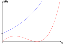
Figure 1: LHS vs. RHS

Besides, LHS grows as $R^{5}$, while RHS grows as $R^{6}$. To conclude the proof, it remains to note that the plots do not intersect for uncountably many sets of parameters $(A_{2},\,A_{5},\,A_{6})$ (e.g., sufficiently small $A_{2}$ and $A_{5}$ with fixed $A_{6}$), therefore $p(r)$ is finite at any point. ∎

So, the solution is defined on the whole real axis for parameter values mentioned above. We now show that the metric extends smoothly to the poles. Since the solution lies on an algebraic curve, it follows that $h(r)$ and $p(r)$ can be expanded as Puiseux series in a neighborhood of $r=0$:

$$\begin{gathered}h(r)=r^{m/n}\sum_{k=0}^{\infty}a_{k}r^{k/n}=r^{m/n}f(r^{1/n}),\\ p(r)=rh_{r}=r^{m/n}\sum_{k=0}^{\infty}\frac{m+k}{n}a_{k}r^{k/n}=r^{m/n}f_{1}(r^{1/n}),\end{gathered}$$ (3.3.2)

where $m\in\mathbb{Z},\,n\in\mathbb{N}$, $f$ and $f_{1}$ are real analytic functions, and $f(0)\neq 0$. Substituting (3.3.2) for $h(r)$ and $p(r)$ in (3.2.4a) one can easily see that the expansions start with the power $-\frac{1}{2}$ or $-\frac{1}{4}$, i.e.

$$\begin{gathered}h(r)=r^{-1/n}f(r^{1/n}),\\ p(r)=r^{-1/n}f_{1}(r^{1/n})\end{gathered}$$ (3.3.3)

with $n=2$ or $4$, and $f_{1}(0)\neq 0$.

Define new coordinates $(\rho,\phi)$ by the formulas $\rho=r^{1/n}=e^{x/n},\,\phi=\dfrac{y}{n}$. In coordinates $(\rho,\phi)$ metric has the form

$$\begin{gathered}g=\frac{1}{h_{x}^{2}}(dx^{2}+dy^{2})=\frac{1}{p^{2}}(n^{2}\,\frac{d\rho^{2}}{\rho^{2}}+n^{2}d\phi^{2})=\frac{n^{2}}{f_{1}(\rho)^{2}}(d\rho^{2}+\rho^{2}d\phi^{2}).\end{gathered}$$ (3.3.4)

Since $f_{1}$ is real analytic and non-vanishing in a neighborhood of the origin $\rho=0$, it follows that the metric $g$ behaves as an ordinary Euclidean metric in polar coordinates, therefore it extends smoothly to the south pole. By changing the sign of $x$ (i.e. switching the poles), it can be proved that the metric extends to the north pole as well.

To show the extensibility of the integrals, consider the following coordinates:

$$\xi=r\cos(y),\quad\eta=r\sin(y)$$ (3.3.5)

and the corresponding momenta $p_{\xi},\,p_{\eta}$. South pole is the origin $(0,\,0)$ in new coordinates. The momenta $p_{x},\,p_{y}$ are given by

$$\begin{gathered}p_{x}=\xi\,p_{\xi}+\eta\,p_{\eta},\\ p_{y}=\xi\,p_{\eta}-\eta\,p_{\xi},\end{gathered}$$ (3.3.6)

It follows that $L=p_{y}$ extends smoothly to the origin. By the pole switching argument $L$ extends also to the north pole.

Quartic integral $F_{1}$ has the following form in new coordinates:

$$\begin{gathered}F_{1}=\left[\xi\eta^{4}+\frac{1}{2}\xi rh_{x}^{2}\Big{(}\eta^{2}(h^{2}+2hh_{x})-2r^{2}h_{x}^{2}-2A_{2}\eta^{2}\Big{)}\right]p_{\xi}^{4}\\ +\left[\frac{\eta^{3}}{2}(1+\eta^{2}-7\xi^{2})-\eta rh_{x}^{2}\left(\xi^{2}(h^{2}+hh_{x})-\eta^{2}hh_{x}-2\xi^{2}A_{2}\right)\right]p_{\xi}^{3}p_{\eta}\\ +\left[-\frac{3}{2}\xi\eta^{2}(1+\eta^{2}-3\xi^{2})-\frac{1}{2}\xi r^{3}h_{x}^{2}\left(4h_{x}^{2}-h^{2}+2A_{2}\right)\right]p_{\xi}^{2}p_{\eta}^{2}\\ +\left[\frac{1}{2}\xi^{2}\eta(3+3\eta^{2}-5\xi^{2})-\eta rh_{x}^{2}\left(\xi^{2}(h^{2}+hh_{x})-\eta^{2}hh_{x}-2\xi^{2}A_{2}\right)\right]p_{\xi}p_{\eta}^{3}\\ +\left[-\frac{\xi^{3}}{2}(1+\eta^{2}-\xi^{2})-\frac{1}{2}\xi rh_{x}^{2}\left(2\eta^{2}hh_{x}-\xi^{2}h^{2}+2r^{2}h_{x}^{2}+2A_{2}\xi^{2}\right)\right]p_{\eta}^{4}.\end{gathered}$$

Since functions $h(r),\,h_{x}(r)$ are of order $r^{-1/2}$ as $r\to 0$, it is sufficient to check that

$$\begin{gathered}h^{2}+2hh_{x},\quad\xi^{2}(h^{2}+hh_{x})-\eta^{2}hh_{x},\quad\xi^{2}h^{2}-2\eta^{2}hh_{x}\end{gathered}$$

have finite limits as $r\to 0$. It follows from the expansions

$$\begin{gathered}h^{2}=c_{0}^{2}r^{-1}+\mbox{r.p.},\\ hh_{x}=-\frac{1}{2}c_{0}^{2}r^{-1}+\mbox{r.p.}\end{gathered}$$

(r.p. stands for the regular part of a series), and identity $r^{2}=\xi^{2}+\eta^{2}$. We see that $F_{1}$ extends smoothly to the south pole. Once again, extensibility to the north pole follows from the pole switching argument.

Continuing this line of reasoning, one can easily find that $F_{2}$ also extends smoothly to the poles. This completes the construction of metrics globally defined on a sphere $S^{2}$.

References

• [1] W. Miller, Jr., S. Post, and P. Winternitz, “Classical and quantum superintegrability with applications,” Journal of Physics A Mathematical General 46 (Oct., 2013) 3001P, arXiv:1309.2694 [math-ph].
• [2] E. Whittaker, A Treatise on the Analytical Dynamics of Particles and Rigid Bodies. Cambridge Mathematical Library. Cambridge University Press, 1988.
• [3] G. Koenigs, Sur les géodesiques a intégrales quadratiques, in: Note II from Darboux’ ‘Leçons sur la théorie générale des surfaces’, vol. IV. Chelsea Publishing, 1896.
• [4] V. S. Matveev and V. V. Shevchishin, “Two-dimensional superintegrable metrics with one linear and one cubic integral,” Journal of Geometry and Physics 61 no. 8, (2011) 1353 – 1377, arXiv:1010.4699 [math-ph].
• [5] G. Valent, C. Duval, and V. Shevchishin, “Explicit metrics for a class of two-dimensional cubically superintegrable systems,” Journal of Geometry and Physics 87 (2015) 461 – 481, arXiv:1403.0422 [math-ph].
• [6] A. V. Bolsinov, V. S. Matveev, and A. T. Fomenko, “Two-dimensional Riemannian metrics with integrable geodesic flows. Local and global geometry,” Sbornik: Mathematics 189 no. 10, (1998) 5–32.
• [7] B. Kruglikov, “Invariant characterization of liouville metrics and polynomial integrals,” Journal of Geometry and Physics 58 no. 8, (2008) 979 – 995, arXiv:0709.0423 [math.DG].