NGTS-2b: An inflated hot-Jupiter transiting a bright F-dwarf

Abstract

We report the discovery of NGTS-2b, an inflated hot-Jupiter transiting a bright F5V star (2MASS J14202949-3112074; $T_{\rm eff}$=$6478^{+94}_{-89}$ K), discovered as part of the Next Generation Transit Survey (NGTS). The planet is in a P=$4.51$ day orbit with mass $0.74^{+0.13}_{-0.12}$ M_J, radius $1.595^{+0.047}_{-0.045}$ R_J and density $0.226^{+0.040}_{-0.038}$ g cm^-3; therefore one of the lowest density exoplanets currently known. With a relatively deep $1.0\%$ transit around a bright V=$10.96$ host star, NGTS-2b is a prime target for probing giant planet composition via atmospheric transmission spectroscopy. The rapid rotation (v sin i=$15.2\pm 0.8$ km s^-1) also makes this system an excellent candidate for Rossiter-McLaughlin follow-up observations, to measure the sky-projected stellar obliquity. NGTS-2b was confirmed without the need for follow-up photometry, due to the high precision of the NGTS photometry.

1 Introduction

Hot-Jupiters are giant exoplanets $(M\gtrsim 0.5$ M_J) orbiting close to their parent stars ($P\lesssim 10$ days). Due to the increased stellar irradiation they experience, hot-Jupiters (hereafter HJs) have higher effective temperatures and larger radii ($1\lesssim R\lesssim 2~{}$R_J) compared to cooler gas giants at larger orbital distances, such as Jupiter (Schneider et al., 2011; Laughlin et al., 2011; Santerne et al., 2016). However, even when accounting for increased stellar irradiation, the radii of many HJs exceed that predicted by evolutionary models (Baraffe et al., 2003; Burrows et al., 2007) and HJs with bulk densities as low as $\sim 0.1$ g cm^-3 have been discovered (Smalley et al., 2012; Hartman et al., 2016). Various internal heating mechanisms have been proposed to reconcile the problem of inflated HJ radii but a proper understanding among the community is still developing (Baraffe et al., 2010; Fortney & Nettelmann, 2010; Baraffe et al., 2014; Thorngren & Fortney, 2018; Sestovic et al., 2018).

HJs transiting bright stars present the finest opportunities for robust exoplanet atmospheric characterisation. The twelve community targets for the James Webb Space Telescope (JWST; Gardner et al. 2006; Kalirai 2018) presented in Stevenson et al. (2016) are all gas giants transiting host stars brighter than $V=12$ with orbital periods $<5$ days. It is therefore important to discover and accurately characterise such systems in advance of JWST operations. Already, comparative atmospheric transmission studies have revealed a diverse range of HJ atmospheres, ranging from clear to cloudy (Sing et al., 2016). Only by discovering new HJs transiting bright stars will we be able to expand these studies and look for statistically significant correlations that may shed light on the formation and evolution of these planets and their atmospheres.

The majority of early exoplanet discoveries were HJs, and although we now recognise that HJs are relatively rare (found around only $\simeq 0.5$% of Sun-like stars Fressin et al., 2013), they still represent important benchmarks for planet formation theories. HJs almost certainly formed at larger orbital separations and migrated to their observed, short-period orbits, but the migration mechanism remains uncertain. Some HJs have orbits that are eccentric and/or misaligned to the stellar rotation axis (see Triaud et al., 2010; Jenkins et al., 2017), and therefore inconsistent with the predictions of disc-driven migration, but the incidence rate of HJs is similarly difficult to reconcile with tidal (“high eccentricity") migration (see the review by Dawson & Johnson, 2018, and references therein). Further detections are therefore crucial if we are to understand how HJs form and evolve.

In this paper we report the discovery of NGTS-2b, a HJ transiting a bright (V=$10.96$) star in a $4.51$ day orbit. In Section 2 we present the NGTS photometric observations that led to the discovery of this planet, as well as the HARPS spectroscopic observations that confirmed the planet and allowed us to determine its mass. In Section 3 we analyse the available data to characterise the system and determine its properties. Finally, in Section 4 we present our conclusions and discuss our results in the context of similar known systems and the opportunities for further follow-up with upcoming space missions.

2 Observations

NGTS-2b was discovered using the NGTS telescopes in conjunction with high precision spectroscopy from HARPS. We detail these observations in this Section.

2.1 NGTS Photometry

NGTS is a wide-field, transit survey located at ESO’s Paranal Observatory in Chile. The primary goal of NGTS is to discover Neptune sized exoplanets orbiting bright (V<13), K and early M-dwarfs – suitable for atmospheric follow-up studies. NGTS comprises an array of twelve fully automated, 20 cm Newtonian telescopes, mounted to independent equatorial forks. Each telescope is coupled to an Andor Ikon-L Camera featuring a 2K$\times$2K e2V deep-depleted, red-sensitive CCD, with 13.5 $\mu$m pixels and an instantaneous field of view of 8 deg². Further details on NGTS can be found in Wheatley et al. (2018).

Field NG1416-3056 was observed by a single NGTS telescope and camera in closed-loop autoguiding mode (McCormac et al., 2013), over a photometric campaign conducted between 2017 January 02 and 2017 August 21. In total 199,324$\,\times$10 s exposures were obtained in the NGTS bandpass (520 – 890 nm) over 139 usable nights. The tracking of the NG1416-3056 field over the 139 nights was stable to an RMS of $0.28$ and $0.11$ pixels in the X and Y directions, respectively.

Raw data were processed by the NGTS pipelines, to obtain systematic detrended light curves for our target object catalogue. A full description of the NGTS pipelines can be found in Wheatley et al. (2018).

2.1.1 Planet detection and vetting

We searched the $\sim$11,000 object light curves from the NG1416-3056 field for transit-like signals using ORION (Wheatley et al., 2018) - an implementation of the box-fitting least squares (BLS) algorithm (Kovács et al., 2002). ORION identified a strong $1.0\%$ depth transit signal for NGTS-2 with a period of $\sim$4.5 days, derived from 12 individual transits. We present the individual transit light curves in Figure 1 and the full light curve, phase-folded to the best fitting period as determined from our global modelling analysis (Section 3.3), in Figure 2. A portion of the full light curve dataset is provided in Table 1.

In order to screen for false-positives mimicking a planetary transit signal, we applied a series of vetting tests. First, we see no evidence of a secondary eclipse at phase 0.5, which would have indicated that the signal is due to an eclipsing stellar companion. Second, we see no depth difference in odd/even numbered transits, which tells us we have identified the true period as opposed to half the true period.

Out of transit ellipsoidal variations are commonly observed for short-period stellar binaries. We do see evidence of sinusoidal variation with a period of $\sim$10.8 hours, which coincides with boundaries between regions of differing data point density. Therefore we attributed the variability to an observation window effect, as opposed to evidence for a stellar binary, a conclusion supported by a low radial velocity amplitude (see Section 2.2).

NGTS-2 has a relatively small proper motion of PM_RA=$-21.736\pm 0.093$ and PM_Dec=$-0.858\pm 0.090$ mas yr^-1 (Gaia Collaboration et al., 2018). Analysis of Gaia sources shows no other objects within the 0.4 arcsec limit of Gaia DR2. Rain diagrams were famously generated for Kepler candidates to identify correlations between photometric flux and centroid time series (Batalha et al., 2010; Bryson et al., 2013). In a similar way, we were able to look for correlations between transit events and shifts in the centre of photometric flux using the method from Günther et al. (2017b). This technique is able to detect false-positive signals due to background contaminating objects within $\sim$1″, much smaller than the size of individual NGTS pixels ($\sim$5″). We find no centroiding correlations down to the milli-pixel level in this case.

Finally, we utilised the astrometric and photometric parameters in Table 3, in conjunction with stellar SED modelling and stellar populations from the Besançon Galaxy model (Robin et al., 2003), to determine that NGTS-2 is an F-dwarf (F5V) rather than an F-giant. This assured us that the observed ($1.0\%$) transit depth can be caused by an occulting body of planetary radius.

We searched for the existence of additional transiting planets around NGTS-2 by masking the transit of NGTS-2b in the NGTS light curve and conducting a series of 5 additional BLS runs. At each step we masked and removed any ‘in-transit’ data points before feeding the remaining data into the next iteration. We searched the period range $0.425$ to $30.0$ days, with a period step of 1 min. We find no other significant BLS detections that resemble a transiting planet in the NGTS light curve.

In conclusion, the planet candidate NGTS-2b passed all of our screening tests and we therefore scheduled the target for spectroscopic follow-up. We note that, in contrast to typical ground-based exoplanet discoveries, follow-up photometry was unnecessary when vetting NGTS-2b owing to the photometric precision of the NGTS light curve (RMS$\sim 2.4$ mmag) in conjunction with the overall rigorous vetting process applied.

Table 1: NGTS photometry for NGTS-2. The full table is available in a machine-readable format from the online journal.

BJDTDB (-2,450,000)	Flux (normalised)	Flux error
7755.83964926	1.001100	0.001087
7755.84844136	0.998410	0.001036
7755.85719473	0.998299	0.0008004
7756.83718233	0.998381	0.001419
7756.84592365	1.003388	0.0009239
7756.85470943	0.999316	0.001139
7756.86076224	1.002791	0.001479
7757.83477136	0.998151	0.001009
7757.84352087	0.997511	0.0007974
7757.85230863	0.998330	0.0007950
…	…	…

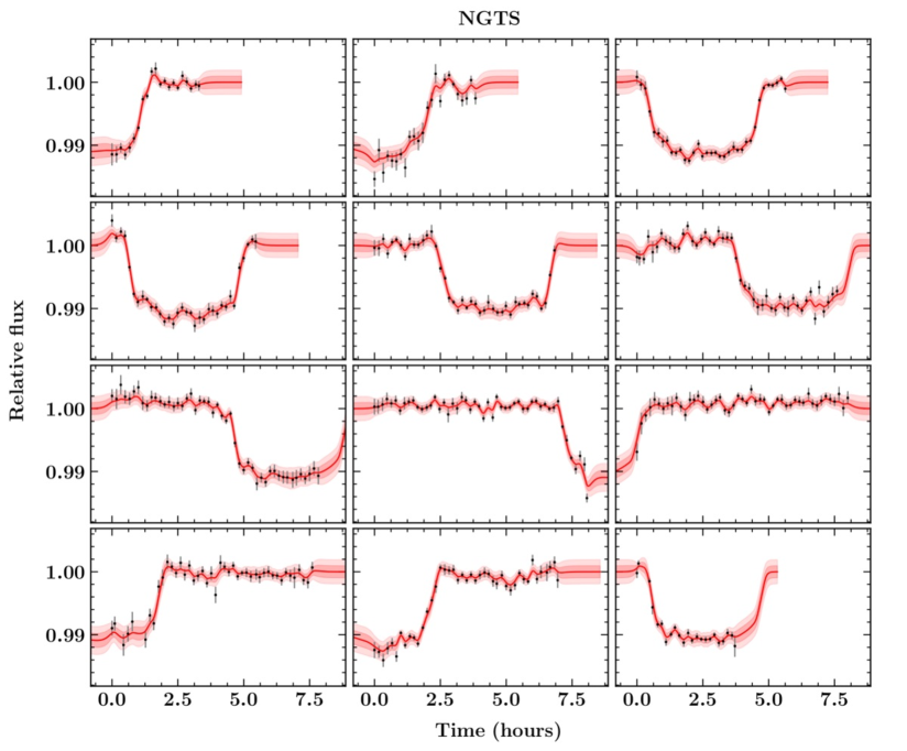
Figure 1: Individual transits of NGTS-2 detected in the NGTS light curve. Black points represent photometric data binned to 10-minute cadence. The red line and pink shaded regions show the median and 1 & 2 $\sigma$ confidence intervals of the posterior model using GP-EBOP (Gillen et al., 2017) set out in Section 3.3, before detrending for the Gaussian process component. The robust detection of NGTS-2b in individual transits (RMS$\sim 2.4$ mmag at 10 minute sampling) demonstrates the high photometric precision of NGTS.

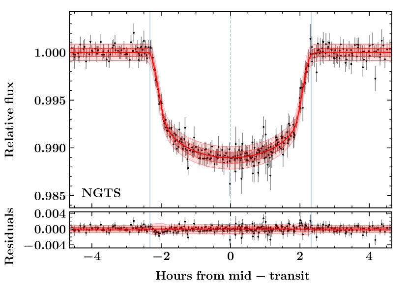
Figure 2: Transit of NGTS-2, phase-folded on the best fitting period as determined from the global modelling set out in Section 3.3. Black points represent photometric data binned to 10-minute cadence. The red line and pink shaded regions show the median and 1 & 2 $\sigma$ confidence intervals of the posterior model using GP-EBOP, which has been detrended for the Gaussian process component. The vertical blue lines represent the transit centre and first and fourth contact points. Residuals are shown below with RMS $\sim 1.3$ mmag.

2.2 Spectroscopy and radial velocities

Spectroscopic data of NGTS-2 were acquired with the HARPS spectrograph (Mayor et al., 2003) on the ESO 3.6 m telescope at La Silla Observatory, Chile under programme 099.C-0303(A) and 0100.C-0474(A). A total of 10 measurements, in High Accuracy Mode (hereafter HAM), were taken between 2017 July 25 and 2017 September 5. An additional 6 measurements were taken in EGGS (high efficiency) mode between 2017 August 17 and 2018 March 12.

Radial velocities (RV) were calculated via cross-correlation with a G2 binary mask, using the standard HARPS reduction pipeline. One measurement was corrected for moonlight contamination, by subtracting the flux from the simultaneous sky fibre. Initial analysis of the RV data showed a variation in phase, consistent with the orbital period and epoch derived from the NGTS photometric data. The semi-amplitude was K$\sim 65$ m s^-1, from which we inferred the existence of a planetary companion.

To ensure that the RV signal does not originate from cool stellar spots or a blended eclipsing binary, we checked for correlations between the line bisector spans and the RV measurements (Figure 3). The bisector span was calculated using a modified version of the standard approach from Queloz et al. (2001), where we disregarded the bottom 20 % of the peak of the cross-correlation function (CCF), while averaging over a greater span. This gives a robust measurement of the asymmetry of the CCF peak, which is less sensitive to local effects caused by stellar pulsation. We find no evidence for a correlation but note a large variation in bisector, suggesting that NGTS-2 is an active or pulsating star.

The RVs, along with associated properties, are detailed in Table 2. We plot the RVs, phase-folded on the best fitting period as determined by our global modelling analysis, in Figure 4.

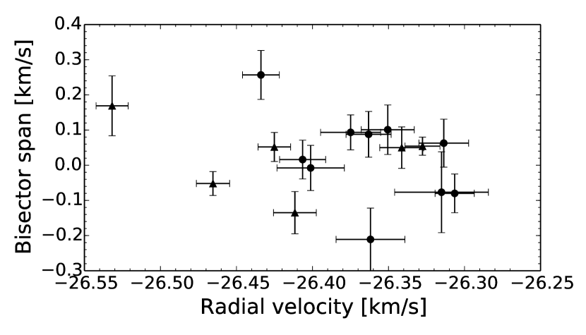
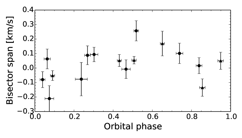
Figure 3: Line bisector span for each HARPS radial velocity measurement, plotted against the measured radial velocity (top panel) and orbital phase (bottom panel). Black points represent HARPS/HAM data points whereas black triangles show HARPS/EGGS mode data. Despite the large variation in bisector span, we find no correlation with the radial velocities.

Table 2: Radial Velocities for NGTS-2, acquired with HARPS on the ESO 3.6m telescope.

BJDTDB	RV	RV error	FWHM	Contrast	BIS	Exptime	Instrument
(-2,450,000)	(km s-1)	(km s-1)	(km s-1)	(%)	(km s-1)	(s)	mode
7959.563593	-26.401	0.022	20.287	12.1	-0.0077	1200	HAM
7960.554740	-26.315	0.031	20.336	12.1	-0.0768	1200	HAM
7962.536130	-26.363	0.015	20.728	12.0	0.0879	1200	HAM
7979.521182	-26.306	0.013	20.800	11.9	-0.0801	2400	HAM
7980.507502	-26.351	0.017	20.644	12.0	0.1010	1200	HAM
7981.537916	-26.434	0.012	20.307	12.1	0.2567	2400	HAM
7997.489848	-26.314	0.016	20.560	12.1	0.0628	2400	HAM
7998.503038	-26.407	0.015	20.566	12.0	0.0161	2400	HAM
8000.503646	-26.375	0.020	20.108	12.2	0.0935	2400	HAM
8002.498343∗	-26.362	0.023	20.328	12.0	-0.2109	2400	HAM
7982.509250	-26.341	0.014	20.241	12.3	0.0500	1200	EGGS
7983.505570	-26.328	0.011	20.100	12.3	-0.0542	1200	EGGS
8160.797565	-26.412	0.014	21.057	11.8	-0.1349	1200	EGGS
8161.832513	-26.465	0.011	20.916	11.9	-0.0520	1200	EGGS
8188.757289	-26.532	0.011	20.466	12.1	0.1690	1200	EGGS
8189.787264	-26.425	0.011	20.276	12.2	0.0519	1200	EGGS

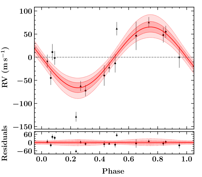
Figure 4: Top: HARPS radial velocity curve of NGTS-2 , phase-folded to the best-fitting period as determined from the global modelling with GP-EBOP set out in Section 3.3. Black points represent HARPS/HAM data points whereas black triangles show HARPS/EGGS mode data. The red line and pink shaded regions show the median and 1 & 2 $\sigma$ confidence intervals of the posterior model. Bottom: Residuals of the fit with RMS $2\%$ and $3\%$ for HAM and EGGS respectively. Error bars and 1 and 2-sigma confidence regions are plotted as in the top panel.

3 Analysis

3.1 Stellar properties

Table 3: Stellar Properties for NGTS-2.

Property	Value	Source
Other Names
2MASS I.D.	J14202949-3112074	2MASS
Gaia I.D.	DR2 6220602384081327104	Gaia
Astrometric Properties
R.A.	14:20:29.5	2MASS
Dec	-31:12:06.68	2MASS
$\mu_{{\rm R.A.}}$ (mas yr-1)	-21.736$\pm$0.093	Gaia
$\mu_{{\rm Dec.}}$ (mas yr-1)	-0.858$\pm$0.090	Gaia
Parallax (mas)	$2.779\pm 0.063$	Gaia
Distance (pc)	$360.3^{+8.3}_{-7.8}$	SED fitting
Photometric Properties
V (mag)	10.961$\pm$0.011	APASS
B (mag)	11.410$\pm$0.02	APASS
g (mag)	11.121$\pm$0.008	APASS
r (mag)	10.878	APASS
i (mag)	10.771$\pm$0.019	APASS
G (mag)	10.860	Gaia
NGTS (mag)	10.790	This work
J (mag)	10.055$\pm$0.023	2MASS
H (mag)	9.858$\pm$0.024	2MASS
Ks (mag)	9.799$\pm$0.021	2MASS
W1 (mag)	9.748$\pm$0.023	WISE
W2 (mag)	9.768$\pm$0.021	WISE
W3 (mag)	9.718$\pm$0.037	WISE
AV	$0.12\pm 0.07$	SED fitting
L${}_{0.1-2.4\,keV}$ (erg s-1)	$\leq$3.74\text{\times}{10}^{30}$$	This work
L${}_{2.0-12.0\,keV}$ (erg s-1)	$\leq$4.49\text{\times}{10}^{31}$$	This work
Lbol (erg s-1)	$$1.76(13)$\times 10^{34}$	SED fitting
Spectral type	F5V	SED fitting
Bulk Properties
$T_{\rm eff}$ (K)	$6478^{+94}_{-89}$	SED fitting
log g (cm s-2)	$4.197^{+0.030}_{-0.059}$	Global modelling
$\rho$ (g cm-3)	$0.477^{+0.030}_{-0.061}$	Global modelling
$\left[Fe/H\right]$	$-0.06\pm 0.09$	HARPS spectra
v sin i (km s-1)	$15.2\pm 0.8$	HARPS spectra
Age (Gyrs)	$2.17\pm 0.37$	HARPS spectra
Mass ($M_{\odot}$)	$1.64^{+0.19}_{-0.22}$	Global modelling
Radius ($R_{\odot}$)	$1.702^{+0.047}_{-0.044}$	SED fitting
2MASS (Skrutskie et al., 2006); APASS (Henden & Munari, 2014)
WISE (Wright et al., 2010); Gaia (Gaia Collaboration et al., 2018)

3.1.1 Bulk properties

To determine stellar bulk properties for NGTS-2 we compared 3 different methods, which we set out in this section. We determined initial stellar parameters by co-adding our individual HARPS (HAM) spectra and measuring equivalent widths, following a similar method to Doyle et al. (2013). Hereafter we refer to this method as Method 1. We obtained the following results: $T_{\rm eff}=6500\pm 100$ K, log g = $4.0\pm 0.2$, [Fe/H] = $-0.06\pm 0.09$ and v sin i = $15.2\pm 0.8$ km s^-1. For v sin i we assumed a macroturbulent velocity ${\it v_{mac}}=6.8\pm 0.7$ km s^-1  based on the asteroseismic calibration of Doyle et al. (2014). No lithium was seen in the spectrum, suggesting NGTS-2 is not a young star.

It is well known that accurate determination of the mass and radius of a transiting exoplanet crucially depends on the accuracy with which one can determine the mass and radius of the stellar host. Historically, stellar host properties for most exoplanets characterised in the literature have been estimated using theoretical models or empirically calibrated relations, as opposed to direct observables, as they have generally provided the greatest accuracy. Using these methods, planetary masses and radii can typically be calculated with uncertainties of 6% and 5%, respectively (Stassun et al., 2017).

To estimate the mass, radius and age of NGTS-2, as well as to check our other parameters are consistent, we also analysed our co-added HARPS spectra with the SPECIES code developed by Soto & Jenkins (2018). Hereafter we refer to this method as Method 2. As in Method 1, SPECIES also uses the measurement of equivalent widths and applies local thermodynamic equilibrium, along with ATLAS9 model atmospheres (Castelli & Kurucz, 2004), to obtain the: temperature, metallicity, surface gravity and micro turbulence of the stellar photosphere. Rotational velocity is found by absorption line fitting with synthetic spectra; the macroturbulent velocity was estimated using the relation from dos Santos et al. (2016). Mass, radius and age are obtained using the isochrones package (Morton, 2015), which interpolates through a grid of MIST isochrones (Dotter, 2016). Photometric properties and parallax from Table 3 are also included as priors in the isochrone interpolation. We obtained the following results for NGTS-2: $T_{\rm eff}$= $6604\pm 134$ K, log g = $4.16^{+0.11}_{-0.09}$ dex, [Fe/H] = $-0.11\pm 0.13$, $M_{*}=1.32^{+0.09}_{-0.08}\,M_{\odot}$, $R_{*}=1.58\pm 0.22\,R_{\odot}$, v sin i = $13.5\pm 1.3$ km s^-1 (assuming ${\it v_{mac}}=7.6\pm 1.3$ km s^-1) and age = 2.17$\pm 0.37$ Gyr.

With the second release of Gaia mission data (DR2), five-parameter astrometric solutions are now available for 1.3 billion sources, with an uncertainty in parallax measurements of up to 0.04 milliarcsecond for G<15 (Gaia Collaboration et al., 2018). For NGTS-2 and other Gaia sources, the most accurate determinations of stellar masses and radii can now be made from direct observables: bolometric flux, effective temperature and parallax; the main uncertainties stem from $T_{\rm eff}$ and $A_{v}$. Using this method, Stassun et al. (2017) reported expected uncertainties in planetary masses and radii of 5% and 3% respectively. Early revisions to the properties of known exoplanets and their host stars, by exploiting this increased accuracy, are starting to appear in the literature. Berger et al. (2018) find a systematic upscaling of planetary radii in the range 1-5 $R_{\oplus}$ and confirm a gap in the radius distribution of small, close-in planets around 2 $R_{\oplus}$ with incident fluxes > 200 $F_{\odot}$.

Utilising direct observables, we modelled the spectral energy distribution (SED) of NGTS-2 (Figure 5), using the broadband photometric method described in Gillen et al. (2017). Hereafter we refer to this method as Method 3. We modelled the SED by convolving PHOENIX v2 model atmospheres with the available bandpasses (see Table 3) and explored the posterior parameter space using Markov chain Monte Carlo (MCMC). The parameters of the fit were the stellar temperature ($T_{\rm eff}$), surface gravity ($\log g$) and radius ($R$), the distance to the system ($d$) and the reddening along the line of sight ($A_{V}$). We also allowed a white noise jitter term ($\ln\sigma$) to account for additional uncertainties above the literature values. For $T_{\rm eff}$ and $\log g$, we used the values from the spectral modelling approach following Doyle et al. (2013) as priors in our fit. The radius, reddening and jitter terms had uninformative priors, and we constrained the distance using the Gaia DR2 parallax value (Bailer-Jones, 2015). We obtain the following results: $T_{\rm eff}$=$6478^{+94}_{-89}$ K, $R_{*}$=$1.702^{+0.047}_{-0.044}$ $R_{\odot}$, $d$=$360.3^{+8.3}_{-7.8}$ pc and $A_{V}=0.12\pm 0.07$. We note that our distance estimate is consistent with the Gaia-derived value presented in Bailer-Jones et al. (2018). See Gillen et al. (2017, and in prep.) for further details of the SED modelling protocol.

In summary, we have calculated stellar parameters from 3 different methods:

1. $T_{\rm eff}$, log g, [Fe/H] and v sin i - from spectral-based method following Doyle et al. (2013), applied to HARPS spectra

2. $T_{\rm eff}$, log g, [Fe/H], v sin i, $M_{*}$, $R_{*}$ and age - from the spectral-based method of Soto & Jenkins (2018) applied to HARPS spectra. Mass, radius and age were determined by interpolating in a grid of isochrones and Gaia parallax and broadband photometry were included as priors

3. $T_{\rm eff}$, log g, $R_{*}$ and distance - from the broadband photometric SED fitting method of Gillen et al. (2017). Gaia DR2 parallax was utilised along with priors on $T_{eff}$ and log g from Method 1.

Comparing our results for NGTS-2 derived using the three different methods, we find that they are consistent within errors. We note that Method 3 (SED fitting) is the most data-driven approach with less dependence on models. Therefore in the remainder of this paper we adopt parameter values according to the following order of precedence:

1. method 3

2. method 1

3. method 2

Specifically, for $T_{\rm eff}$ and $R_{*}$ - we adopt values from Method 3; for [Fe/H] and vsini - we adopt values from Method 1; only Method 2 produced a value for age.

We have determined initial stellar parameters independently of the planet/system. In Section 3.3 we subsequently consider the system as a whole to derive additional parameters. We apply global (simultaneous) modelling of all the data sets, incorporating the adopted values derived in this section as priors. We derive the stellar density from the best fitting transit model parameters, and combine the density with the stellar radius to calculate the stellar mass ($M_{*}$) and to further constrain log g. The final stellar parameters are summarised in Table 3 with corresponding sources.

We investigated the X-ray brightness of the host star and found that no detection has yet been made at the source position. Nevertheless, using ROSAT and XMM-Newton slew images we were able to determine upper limits for the luminosity of $\sim$3.73\text{\times}{10}^{30}$$ erg s^-1 in the 0.1–2.4 keV band and $\sim$4.47\text{\times}{10}^{31}$$ erg s^-1 in the 2.0–12.0 keV band. As such, we conclude that NGTS-2 is fainter than a small percentage of the brighter F stars seen but cannot rule out that NGTS-2 itself is still among the brightest (Panzera et al., 1999).

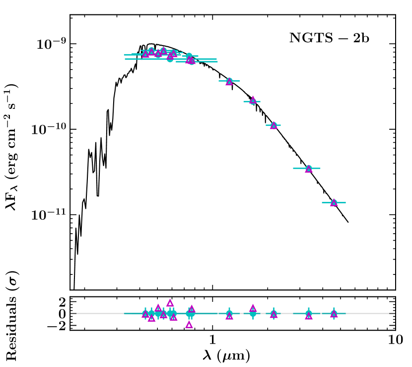
Figure 5: The fitted spectral energy distribution (black line) for NGTS-2 based on the photometric data (cyan points) presented in Table 3 using the method presented in Gillen et al. (2017). The black line shows the best fit model atmosphere and the magenta triangles show the model flux at the wavelengths of the photometric data. Bottom: Residuals of the fit in units of observational uncertainty.

3.1.2 Kinematics

Considering the proper motion (R.A.:$-21.736\pm 0.093$ mas yr^-1, Dec.: $-0.858\pm 0.090$ mas yr^-1), the absolute radial velocity ($-26.3616^{+0.0064}_{-0.0063}$ km s^-1), and the parallax distance of $360.3^{+8.3}_{-7.8}$ pc, we calculate the ($U_{LSR},V_{LSR},W_{LSR}$) galactic motion for NGTS-2 to be ($30.048\pm 0.028$, $25.781\pm 0.020$, $-5.093\pm 0.018$) km s^-1. Given that these velocity vector components are small, this suggests that NGTS-2 is a member of the thin disk population.

3.2 Stellar Activity and Rotation

Knowledge of the stellar rotation period and activity properties of exoplanet host stars are valuable for a number of reasons. On the one-hand, activity can act as a nuisance in the radial velocity follow-up of transiting planets, since plage and starspots can manifest themselves as apparent RV shifts that can mask or (in extreme cases) mimic orbiting planets (e.g. Queloz et al., 2001; Huélamo et al., 2008). In addition, the presence of unocculted spots in transit lightcurves can also systematically bias the determined planetary radii (e.g. Désert et al., 2011; Sing et al., 2011). Hence understanding stellar activity can help counter such issues, thereby improving the veracity of the measured planetary parameters such as mass and radius. However, magnetic activity may also reveal the stellar rotation period, enabling additional important properties of the star and the planetary system as a whole to be constrained. For example, this includes system aging via gyrochronology (e.g. Barnes, 2007; Barnes et al., 2016), as well as permitting highly misaligned transiting planetary systems to be identified through determination of the inclination of the stellar spin axis without the need for Rossiter-McLaughlin observations (e.g. Watson et al., 2010; Simpson et al., 2010; Schlaufman, 2010).

3.2.1 Spectroscopic constraints

While NGTS-2 is a moderately rapid rotator with a $v\sin i_{*}$ of $15.2\pm 0.8$ km s^-1(and hence has the potential to be an active star), this possibility is offset by its relatively early spectral type (F5V). This places it close to the boundary where the dynamo generating tacholine may not operate efficiently due to an extremely shallow outer convective envelope. However, the stellar parameters (see Table 3) allow an estimate of the expected stellar rotation period ($P_{rot}$) independent of the presence of rotationally modulated activity via:

$$P_{rot}=\bigg{(}\frac{2\pi R_{*}}{v\sin i_{*}}\bigg{)}\sin i_{*}$$ (1)

where $R_{*}$, $v$ and $i_{*}$ are the stellar radius, stellar rotational velocity and inclination of the stellar rotation axis, respectively. Assuming spin-orbit alignment ($i_{*}$ = 90^∘), this results in $P_{rot}$ = $5.66^{+0.49}_{-0.44}$days – which also represents the upper limit to $P_{rot}$.

3.2.2 Photometric constraints

We performed a detailed search for the signal of a photometric rotation period in NGTS data. In this analysis, the transits of NGTS-2b were removed (just leaving the out-of-transit light) prior to pre-whitening to also remove integer 1- and 2-day periods that occur due to the observing window function.

Figure 6 shows the generalised Lomb Scargle (GLS) periodogram spanning 1.2–10 days (thought to encompass the likely rotation period of NGTS-2 – see earlier), along with a false alarm probability (FAP) calculated using 1,000 bootstraps of the NGTS photometry in order to sample the window function in that period range. This shows a main peak at 7.25 days, with the next strongest peak lying at 3.97 days (as well as a forest of other signals, predominantly at lower periods). We carried out a wavelet analysis of the same data but binned into $\sim$15 minute intervals to allow for a constant time interval required for wavelet analysis (Torrence & Compo, 1998). Gaps in the data were left as is, and this does not have a considerable effect on the resultant power spectrum.

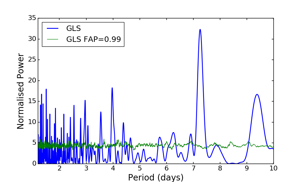
Figure 6: Generalised Lomb Scargle Periodogram for NGTS-2, after detrending for the window function and removal of transit signals. There are strong signals at 7.25 and 3.97 days.

Both the wavelet and GLS show signals at $\sim$7.2 and 3–4 days, although 7.2 days is not consistent with the estimated rotational period, which constitutes an upper limit of $5.66^{+0.49}_{-0.44}$days. The wavelet analysis shows two distinct timespans where these signals are strongest (from $\sim$70 – 120 days, and again from $\sim$150 – 200 days). We have phase-folded the NGTS light-curves on the prominent periods for the entire dataspan, as well as only for times when the wavelet analysis indicated high power at those periods. We see no clear evidence of a rotationally modulated signal in any of these phase folded light curves.

A median periodogram was produced for the $\sim$11,000 other stars within the same NGTS field as NGTS-2, observed in the same season and with the same camera. This shows a very broad, minor peak covering periods between $\sim$6 and $\sim$8 days, significant periodicity around $\sim$4 days, as well as a forest of power at shorter periods.

We conclude that the observed peaks for NGTS-2 at $\sim$4 days and 7.2 days likely arise due to systematics. We see no convincing evidence for a rotational period of NGTS-2 in the NGTS light curve, which is consistent with the estimated value irrespective of whether the system is aligned or misaligned.

3.3 Global Modelling

Intrinsic stellar variability (Section 3.2) and residual observational systematics can give rise to time correlated (“red”) noise in photometric light curves, which can subtly alter the shape of transits leading to inaccurate model fitting (Pont et al., 2006; Pont et al., 2008; Silva-Valio, 2008).

Given the presence of correlated noise (likely stellar and systematic) in the NGTS light curve, we globally modelled NGTS-2 using GP-EBOP (Gillen et al., 2017) to constrain the stellar and planetary parameters. GP-EBOP comprises a central EBOP-based transiting planet and eclipsing binary model, which is wrapped within a Gaussian process (GP) model. The GP is designed to robustly account for stellar activity and instrumental systematics, and propagate uncertainties due to these into the posterior distributions of the stellar and planetary parameters. GP-EBOP explores the posterior parameter space using EMCEE (Foreman-Mackey et al., 2013). The interested reader is referred to Gillen et al. (2017) for further details of GP-EBOP’s modelling protocol.

Before modelling with GP-EBOP, the detrended NGTS light curve was normalised by the median out-of-transit flux and binned to 10 mins cadence. A quadratic limb darkening law was utilised (Kopal 1950; Mandel & Agol 2002) with the profiles and uncertainties obtained via the LDTk package (Husser et al., 2013; Parviainen & Aigrain, 2015). LDTk was given estimates of $T_{\rm eff}$, $\log g$ and [Fe/H] from our SED modelling and the spectral modelling method of Doyle et al. (2013). The resultant uncertainty in the limb darkening profile was inflated by a factor of 10 to account for systematic errors in the stellar atmosphere models in the region of parameter space where NGTS-2 lies.

We fitted for an systemic radial velocity offset between HARPS/HAM and HARPS/EGGS modes. In addition to the offset, GP-EBOP also allows for stellar and systematic RV jitter above the observational uncertainties, with data from each instrument treated individually. Given the relatively short orbital period of NGTS-2b, theoretical and empirical evidence of single systems would favour a circular orbit (Anderson et al., 2012). Furthermore, the observational RV uncertainties likely preclude a robust detection of eccentricity below a moderate value. Nevertheless we compared a circular orbit model (e=0) with a model where eccentricity was free to vary.

In both cases, we stepped through the parameter space 50,000 times with each of 150 walkers (conservatively discarding the first 30,000 steps as burn in). Walkers were initialised from within a representative region of parameter space. Chains were thinned by a factor of 100 to reduce clustered samples, unrepresentative of the true posterior distribution, due to autocorrelation. Finally, the Gelman-Rubin criterion (Gelman & Rubin, 1992) was used to check chain convergence.

Comparing the results from the eccentric and circular models, we reassuringly find consistent results for our parameters of interest. However, we note that the eccentricity is not well constrained ($e=0.035^{+0.106}_{-0.031}$). Given the lack of secondary eclipse, the main constraint on eccentricity is given by the RV data, which have large uncertainties ($\sim 20$ m s^-1). We identified two families of low eccentricity solution, which are compatible with the data, differing in their eccentricity combination terms but not their overall eccentricity value. The eccentricity value and uncertainty should therefore be treated with caution and thus we adopt the circular model as our main model.

We find that NGTS-2 is orbited by NGTS-2b with semi-major axis a=$0.0630^{+0.0024}_{-0.0030}$ AU and inclination i=$88.5^{+1.0}_{-1.2}$ deg. NGTS-2b has a mass $0.74^{+0.13}_{-0.12}$ M_J, radius $1.595^{+0.047}_{-0.045}$ R_J and density $0.226^{+0.040}_{-0.038}$ g cm^-3. Assuming an albedo equal to that of Jupiter, we calculate an equilibrium temperature for NGTS-2b of $1468^{+45}_{-42}$ K but note that such assumption has a large uncertainty given the lack of knowledge of the planetary atmosphere (Borucki et al., 2011). Interestingly, we emphasise that this is a low planetary density for a HJ and discuss this in Section 4. In agreement with previous estimates from spectral based methods, we determine a stellar mass and log g for NGTS-2 of $1.64^{+0.19}_{-0.22}$ $M_{\odot}$ and $4.197^{+0.030}_{-0.059}$ g cm^-3 respectively, by combining the adopted stellar radius from SED fitting with the stellar density measured directly from the posterior parameters. We adopt these values as the final mass and log g for NGTS-2 and include them in the summary table of stellar properties (Table 3). Fitted and derived parameters from our global modelling are presented in Table 4.

Table 4: Planetary and system parameters from global modelling of the NGTS-2 system. The results from fixed eccentricity (e=0) versus floating eccentricity fitting are compared. The median values of the posterior distributions were adopted as the most probable parameters, with the $1\sigma$ intervals as the error estimates. We present results from the circular orbit (e=0) scenario as our main results (see Section 3.3 for explanation).

Parameter	Description	Unit	Value
			Fixed e=0	Floating e
Fitted parameters
$\frac{R+r}{a}$	Sum of radii relative to semi-major axis of system	none	$0.1369^{+0.0065}_{-0.0028}$	$0.1377^{+0.0080}_{-0.0037}$
$k$	radius ratio planet to star, $\frac{r}{R}$	none	$0.09619^{+0.00114}_{-0.00088}$	$0.09633^{+0.00136}_{-0.00097}$
$\cos i$	cosine of orbital inclination	none	$0.026^{+0.021}_{-0.018}$	$0.030^{+0.023}_{-0.021}$
$\sqrt{e}\cos\omega$	orbital eccentricity and argument of periastron term	none		$0.00^{+0.10}_{-0.13}$
$\sqrt{e}\sin\omega$	orbital eccentricity and argument of periastron term	none		$0.050^{+0.093}_{-0.326}$
$P$	orbital period	days	$4.511164\pm 0.000061$	$4.511164^{+0.000070}_{-0.000069}$
$T_{c}$	epoch of transit centre	BJD	$2457759.1261^{+0.0014}_{-0.0013}$	$2457759.1259^{+0.0016}_{-0.0017}$
$q1_{\rm{NGTS}}$	first Kipping LD term ∗	none	$0.3431^{+0.0072}_{-0.0071}$	$0.3431^{+0.0073}_{-0.0072}$
$q2_{\rm{NGTS}}$	second Kipping LD term ∗	none	$0.3903^{+0.0055}_{-0.0054}$	$0.3904\pm 0.0055$
$\ln(\sigma^{2})_{\rm{HAM}}$	natural log of jitter in HAM RV data	ln(km${}^{2}\,s^{-2}$)	$-10.6^{+2.6}_{-6.3}$	$-10.3^{+2.5}_{-6.3}$
$\ln(\sigma^{2})_{\rm{EGGS}}$	natural log of jitter in EGGS RV data	ln(km${}^{2}\,s^{-2}$)	$-6.56^{+0.85}_{-0.73}$	$-6.52^{+0.83}_{-0.74}$
$K$	radial velocity semi-amplitude of star	m s-1	$65.8^{+9.5}_{-9.1}$	$66.1^{+9.8}_{-9.2}$
$V_{\rm{sys}}$	systemic velocity	km s-1	$-26.3616^{+0.0064}_{-0.0063}$	$-26.3615^{+0.0063}_{-0.0064}$
$\delta$V${}_{\rm{sys~{}EGGS}}$	EGGS RV mode offset	m s-1	$41^{+19}_{-18}$	$41^{+18}_{-19}$
$\ln(A^{2})_{\rm NGTS}$	natural log of squared amplitude $\ddagger$	ln(rel. flux2)	$-13.90\pm 0.13$	$-13.89\pm 0.13$
$\ln(l^{2})_{\rm NGTS}$	natural log of squared timescale $\ddagger$	ln(days2)	$-9.36^{+0.32}_{-0.30}$	$-9.37^{+0.34}_{-0.31}$
$\ln(\sigma^{2})_{\rm NGTS}$	natural log of variance $\ddagger$	ln(rel. flux2)	$-29.7^{+6.9}_{-7.0}$	$-29.8^{+6.8}_{-6.9}$
Derived parameters
$e$	orbital eccentricity	none		$0.035^{+0.106}_{-0.031}$
$i$	orbital inclination	$deg$	$88.5^{+1.0}_{-1.2}$	$88.3^{+1.2}_{-1.3}$
$a$	semi-major axis of system	AU	$0.0630^{+0.0024}_{-0.0030}$	$0.0628^{+0.0026}_{-0.0035}$
$r$	radius of planet	$R_{jup}$	$1.595^{+0.047}_{-0.045}$	$1.598^{+0.048}_{-0.046}$
$m$	mass of planet	$M_{jup}$	$0.74^{+0.13}_{-0.12}$	$0.76^{+0.17}_{-0.15}$
$\rho$	density of planet	g cm-3	$0.226^{+0.040}_{-0.038}$	$0.232^{+0.054}_{-0.048}$
$T_{eq}$	equilibrium temperature of planet	$K$	$1468^{+45}_{-42}$	$1472^{+50}_{-44}$
$T_{14}$	transit duration	hours	$4.651^{+0.046}_{-0.038}$	$4.67^{+0.38}_{-0.11}$

4 Discussion and conclusion

With a radius of $1.595^{+0.047}_{-0.045}$ R_J, mass $0.74^{+0.13}_{-0.12}$ M_J and equilibrium temperature $1468^{+45}_{-42}$ K, NGTS-2b is an inflated HJ (Figure 3 & 8). In fact the density of NGTS-2b is only $0.226^{+0.040}_{-0.038}$ g cm^-3, placing it among the least dense planets known. Orbiting with period $4.51$ days, NGTS-2b is slightly further from its stellar host than most HJs with similar densities and host spectral types. For instance, WASP-121b (Delrez et al., 2016) orbits its F6V star much closer in, with period 1.27 days.

Other HJs with masses and radii similar to NGTS-2b include WASP-90b (West et al., 2016), WASP-118b (Hay et al., 2016; Močnik et al., 2017) and WASP-88b (Delrez et al., 2014). The lower density of these planets suggests a planetary heating mechanism is at play, which is independent of stellar irradiation. Plausible explanations could include increased internal heat generation (Ginzburg & Sari, 2015), double-diffusive convection (Leconte & Chabrier, 2012) and increased atmospheric opacity (Burrows et al., 2007). In order to properly ascertain the causes of HJ inflation, the sample of inflated planets with precisely measured masses and radii must be expanded, allowing trends to be discerned which distinguish the competing theories.

Characterisation of exoplanet atmospheres via transmission spectroscopy has been carried out for bright targets using HARPS (Wyttenbach et al., 2015), ESPRESSO (Pepe et al., 2010) and HST (Sing et al., 2016). The JWST, scheduled for launch in 2020, will further enable atmospheric measurements at a higher level of precision (Beichman et al., 2014; Stevenson et al., 2016). NGTS-2b is a short-period gas giant orbiting a bright (V$\sim$11) stellar host. In addition, we calculate an atmospheric scale height of $\sim 760$ km. These properties make NGTS-2b an ideal target for such studies.

Previous work has shown that the orbits of hot and warm Jupiters around early-type stars are often misaligned with the stellar rotation axis (e.g., Winn & Fabrycky, 2015). The effective temperature of NGTS-2 ($6478^{+94}_{-89}$ K) is hotter than the empirical boundary of $\simeq$6250 K, above which high orbital obliquities are common (particularly for giant planets with $M\lesssim 3$M_J). We were not able to determine a convincing rotational period of NGTS-2 from our photometric and spectroscopic analysis (Section 3.2), accordingly we cannot confirm whether there is spin-orbit misalignment in the NGTS-2 system. We recommend Rossiter-McLaughlin follow-up observations and note that either outcome (aligned or misaligned) is interesting for the stellar type of NGTS-2. The brightness of the host star combined with the rapid stellar rotation should make the effect readily detectable. Using Eq. (40) from Winn (2010) we calculate a maximum amplitude for the signal of $110$ m s^-1, which is an order of magnitude larger than our typical HARPS RV measurement error of $\sim 20$ m s^-1.

The Transiting Exoplanet Survey Satellite (TESS; Ricker et al. 2014) has recently launched, with the Guest Investigator Program allowing observations to be made outside of the mission’s core science operations. We searched for, and found no evidence of, multiple planets in the NGTS-2 system. As a space-borne observatory, TESS’ increased photometric precision over ground-based facilities is more equipped to search for additional (and shallower) transit signals, indicative of other planets in this system besides NGTS-2b. The presence of multiple planets can also be inferred from Transit Timing Variations (TTVs), as was achieved with K2 observations of WASP-47 (Becker et al., 2015). The 2 minute cadence would be required for robust TTVs.

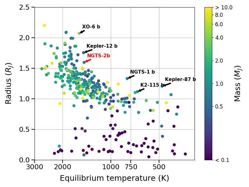
Figure 7: Parameter space of planetary radius versus planetary equilibrium temperature, for confirmed exoplanets. Planetary mass is indicated by the colour-bar scale. The location of NGTS-2 is shown by a red arrow, assuming an albedo equal to that of Jupiter, while a selection of inflated planets are shown by black arrows. The combination of lower temperature, lower mass but higher radius of NGTS-2b, compared to the distribution of planets, highlights that NGTS-2b is inflated.

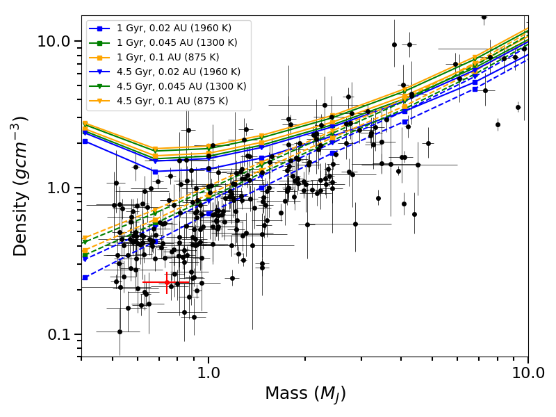
Figure 8: Planetary density versus planetary mass, for previously confirmed HJs¹ (black data points) and NGTS-2b (red data point). Theoretical relations from Fortney et al. (2007) are plotted for comparison, considering planetary evolution under stellar irradiation. We plot theoretical relations for planet ages, orbital separations and effective temperatures similar to NGTS-2b. Dashed lines depict planets with $100~{}M_{\oplus}$ cores, where as solid lines represent planets with no cores. The density of NGTS-2b exceeds the theoretical values for a planet of the same age and effective temperature, irrespective of its composition. This suggests additional heating mechanisms, which are not considered in the theoretical models, are contributing to the atmospheric heating of NGTS-2b.

In conclusion we have discovered NGTS-2b, an inflated hot-Jupiter (M_p=$0.74^{+0.13}_{-0.12}$ M_J, R_p=$1.595^{+0.047}_{-0.045}$ R_J, $\rho_{p}$=$0.226^{+0.040}_{-0.038}$ g cm^-3) transiting a bright F5V star in a $4.51$ day orbit. NGTS-2b is one of the least dense exoplanets currently known. Selection of this ideal target for future follow-up studies may advance our understanding of the formation and evolution of hot-Jupiters and their atmospheres.

The considerable power of NGTS as an exoplanet survey facility, has been demonstrated by confirming NGTS-2b without the need for follow-up photometry. Over a 4 year period, NGTS is expected to yield $\sim$ 200 planets larger than Neptune and more importantly $\sim$10 smaller planets (Günther et al., 2017a), all orbiting bright hosts. In the era of TESS, NGTS will undoubtedly play a crucial role in candidate follow-up. The enhanced plate scale of NGTS (5 arcsec pixel^-1) compared to TESS (21 arcsec pixel^-1) will allow better separation of blended targets in the TESS fields. In addition, based on noise models for a 1 hour sampling rate (Ricker et al. 2014; Wheatley et al. 2018) NGTS is expected to achieve higher photometric precision than TESS for magnitudes fainter than $I=14$, owing to its larger aperture.

Affiliations

^lDepartment of Physics and Astronomy, Leicester Institute of Space and Earth Observation, University of Leicester, LE1 7RH, UK
^cCavendish Laboratory, J.J. Thomson Avenue, Cambridge CB3 0HE, UK
^dInstitute of Planetary Research, German Aerospace Center, Rutherfordstrasse 2, 12489 Berlin, Germany
^wDept. of Physics, University of Warwick, Gibbet Hill Road, Coventry CV4 7AL, UK
^ceCentre for Exoplanets and Habitability, University of Warwick, Gibbet Hill Road, Coventry CV4 7AL, UK
^gObservatoire de Genève, Université de Genève, 51 Ch. des Maillettes, 1290 Sauverny, Switzerland
^qAstrophysics Research Centre, School of Mathematics and Physics, Queen’s University Belfast, BT7 1NN Belfast, UK
^caInstitute of Astronomy, University of Cambridge, Madingley Rise, Cambridge CB3 0HA, UK
^ucDepartamento de Astronomia, Universidad de Chile, Casilla 36-D, Santiago, Chile
^ci Centro de Astrofísica y Tecnologías Afines (CATA), Casilla 36-D, Santiago, Chile.
^aInstituto de Astronomia, Universidad Católica del Norte, Casa Central, Angamos 0610, Antofagasta, Chile
^fuInstitute of Geological Sciences, FU Berlin, Malteserstr. 74-100, D-12249 Berlin, Germany
^tuCenter for Astronomy and Astrophysics, TU Berlin, Hardenbergstr. 36, D-10623 Berlin, Germany
^kAstrophysics Group, Lennard-Jones Laboratories, Keele University, Staffordshire ST5 5BG, UK
^rsDr. Remeis-Sternwarte, Friedrich Alexander Universität Erlangen-Nürnberg, Sternwartstr. 7, 96049 Bamberg, Germany
^† Winton Fellow

References

- Anderson et al. (2012) Anderson D. R., et al., 2012, MNRAS, 422, 1988
- Bailer-Jones (2015) Bailer-Jones C. A. L., 2015, Publications of the Astronomical Society of the Pacific, 127, 994
- Bailer-Jones et al. (2018) Bailer-Jones C. A. L., Rybizki J., Fouesneau M., Mantelet G., Andrae R., 2018, preprint, (arXiv:1804.10121)
- Baraffe et al. (2003) Baraffe I., Chabrier G., Barman T. S., Allard F., Hauschildt P. H., 2003, A&A, 402, 701
- Baraffe et al. (2010) Baraffe I., Chabrier G., Barman T., 2010, Reports on Progress in Physics, 73, 016901
- Baraffe et al. (2014) Baraffe I., Chabrier G., Fortney J., Sotin C., 2014, Protostars and Planets VI, pp 763–786
- Barnes (2007) Barnes S. A., 2007, ApJ, 669, 1167
- Barnes et al. (2016) Barnes S. A., Weingrill J., Fritzewski D., Strassmeier K. G., Platais I., 2016, ApJ, 823, 16
- Batalha et al. (2010) Batalha N. M., et al., 2010, ApJ, 713, L103
- Becker et al. (2015) Becker J. C., Vanderburg A., Adams F. C., Rappaport S. A., Schwengeler H. M., 2015, ApJ, 812, L18
- Beichman et al. (2014) Beichman C., et al., 2014, PASP, 126, 1134
- Berger et al. (2018) Berger T. A., Huber D., Gaidos E., van Saders J. L., 2018, preprint, (arXiv:1805.00231)
- Borucki et al. (2011) Borucki W. J., Koch D. G., Basri G., Batalha N., Brown et al., 2011, ApJ, 736, 19
- Bryson et al. (2013) Bryson S. T., et al., 2013, Publications of the Astronomical Society of the Pacific, 125, 889
- Burrows et al. (2007) Burrows A., Hubeny I., Budaj J., Hubbard W. B., 2007, ApJ, 661, 502
- Castelli & Kurucz (2004) Castelli F., Kurucz R. L., 2004, ArXiv Astrophysics e-prints,
- Dawson & Johnson (2018) Dawson R. I., Johnson J. A., 2018, preprint, (arXiv:1801.06117)
- Delrez et al. (2014) Delrez L., et al., 2014, A&A, 563, A143
- Delrez et al. (2016) Delrez L., et al., 2016, MNRAS, 458, 4025
- Désert et al. (2011) Désert J.-M., et al., 2011, A&A, 526, A12
- Dotter (2016) Dotter A., 2016, ApJS, 222, 8
- Doyle et al. (2013) Doyle A. P., et al., 2013, MNRAS, 428, 3164
- Doyle et al. (2014) Doyle A. P., Davies G. R., Smalley B., Chaplin W. J., Elsworth Y., 2014, MNRAS, 444, 3592
- Foreman-Mackey et al. (2013) Foreman-Mackey D., Hogg D. W., Lang D., Goodman J., 2013, Publications of the Astronomical Society of the Pacific, 125, 306
- Fortney & Nettelmann (2010) Fortney J. J., Nettelmann N., 2010, Space Sci. Rev., 152, 423
- Fortney et al. (2007) Fortney J. J., Marley M. S., Barnes J. W., 2007, ApJ, 659, 1661
- Fressin et al. (2013) Fressin F., et al., 2013, ApJ, 766, 81
- Gaia Collaboration et al. (2018) Gaia Collaboration Brown A. G. A., Vallenari A., Prusti T., de Bruijne J. H. J., Babusiaux C., Bailer-Jones C. A. L., 2018, preprint, (arXiv:1804.09365)
- Gardner et al. (2006) Gardner J. P., et al., 2006, Space Sci. Rev., 123, 485
- Gelman & Rubin (1992) Gelman A., Rubin D. B., 1992, Statist. Sci., 7, 457
- Gillen et al. (2017) Gillen E., Hillenbrand L. A., David T. J., Aigrain S., Rebull L., Stauffer J., Cody A. M., Queloz D., 2017, ApJ, 849, 11
- Ginzburg & Sari (2015) Ginzburg S., Sari R., 2015, ApJ, 803, 111
- Günther et al. (2017a) Günther M. N., Queloz D., Demory B.-O., Bouchy F., 2017a, MNRAS, 465, 3379
- Günther et al. (2017b) Günther M. N., et al., 2017b, MNRAS, 472, 295
- Hartman et al. (2016) Hartman J. D., et al., 2016, AJ, 152, 182
- Hay et al. (2016) Hay K. L., et al., 2016, MNRAS, 463, 3276
- Henden & Munari (2014) Henden A., Munari U., 2014, Contributions of the Astronomical Observatory Skalnate Pleso, 43, 518
- Huélamo et al. (2008) Huélamo N., et al., 2008, A&A, 489, L9
- Husser et al. (2013) Husser T.-O., Wende-von Berg S., Dreizler S., Homeier D., Reiners A., Barman T., Hauschildt P. H., 2013, A&A, 553, A6
- Jenkins et al. (2017) Jenkins J. S., et al., 2017, MNRAS, 466, 443
- Kalirai (2018) Kalirai J., 2018, Contemporary Physics, 59, 251
- Kipping (2013) Kipping D. M., 2013, MNRAS, 435, 2152
- Kopal (1950) Kopal Z., 1950, Harvard College Observatory Circular, 454, 1
- Kovács et al. (2002) Kovács G., Zucker S., Mazeh T., 2002, A&A, 391, 369
- Laughlin et al. (2011) Laughlin G., Crismani M., Adams F. C., 2011, ApJ, 729, L7
- Leconte & Chabrier (2012) Leconte J., Chabrier G., 2012, A&A, 540, A20
- Mandel & Agol (2002) Mandel K., Agol E., 2002, ApJ, 580, L171
- Mayor et al. (2003) Mayor M., et al., 2003, The Messenger, 114, 20
- McCormac et al. (2013) McCormac J., Pollacco D., Skillen I., Faedi F., Todd I., Watson C. A., 2013, PASP, 125, 548
- Morton (2015) Morton T. D., 2015, isochrones: Stellar model grid package, Astrophysics Source Code Library (ascl:1503.010)
- Močnik et al. (2017) Močnik T., Hellier C., Anderson D. R., Clark B. J. M., Southworth J., 2017, MNRAS, 469, 1622
- Panzera et al. (1999) Panzera M. R., Tagliaferri G., Pasinetti L., Antonello E., 1999, A&A, 348, 161
- Parviainen & Aigrain (2015) Parviainen H., Aigrain S., 2015, MNRAS, 453, 3821
- Pepe et al. (2010) Pepe F. A., et al., 2010, in Ground-based and Airborne Instrumentation for Astronomy III. p. 77350F, doi:10.1117/12.857122
- Pont et al. (2006) Pont F., Zucker S., Queloz D., 2006, MNRAS, 373, 231
- Pont et al. (2008) Pont F., Knutson H., Gilliland R. L., Moutou C., Charbonneau D., 2008, MNRAS, 385, 109
- Queloz et al. (2001) Queloz D., et al., 2001, A&A, 379, 279
- Ricker et al. (2014) Ricker G. R., et al., 2014, in Society of Photo-Optical Instrumentation Engineers (SPIE) Conference Series. p. 20 (arXiv:1406.0151), doi:10.1117/12.2063489
- Robin et al. (2003) Robin A. C., Reylé C., Derrière S., Picaud S., 2003, A&A, 409, 523
- Santerne et al. (2016) Santerne A., et al., 2016, A&A, 587, A64
- Schlaufman (2010) Schlaufman K. C., 2010, ApJ, 719, 602
- Schneider et al. (2011) Schneider J., Dedieu C., Le Sidaner P., Savalle R., Zolotukhin I., 2011, A&A, 532, A79
- Sestovic et al. (2018) Sestovic M., Demory B.-O., Queloz D., 2018, preprint, p. arXiv:1804.03075 (arXiv:1804.03075)
- Silva-Valio (2008) Silva-Valio A., 2008, ApJ, 683, L179
- Simpson et al. (2010) Simpson E. K., Baliunas S. L., Henry G. W., Watson C. A., 2010, MNRAS, 408, 1666
- Sing et al. (2011) Sing D. K., et al., 2011, MNRAS, 416, 1443
- Sing et al. (2016) Sing D. K., et al., 2016, Nature, 529, 59
- Skrutskie et al. (2006) Skrutskie M. F., et al., 2006, AJ, 131, 1163
- Smalley et al. (2012) Smalley B., et al., 2012, A&A, 547, A61
- Soto & Jenkins (2018) Soto M. G., Jenkins J. S., 2018, preprint, (arXiv:1801.09698)
- Stassun et al. (2017) Stassun K. G., Collins K. A., Gaudi B. S., 2017, AJ, 153
- Stevenson et al. (2016) Stevenson K. B., et al., 2016, PASP, 128, 094401
- Thorngren & Fortney (2018) Thorngren D. P., Fortney J. J., 2018, AJ, 155, 214
- Torrence & Compo (1998) Torrence C., Compo G. P., 1998, Bulletin of the American Meteorological Society, 79, 61
- Triaud et al. (2010) Triaud A. H. M. J., et al., 2010, A&A, 524, A25
- Watson et al. (2010) Watson C. A., Littlefair S. P., Collier Cameron A., Dhillon V. S., Simpson E. K., 2010, MNRAS, 408, 1606
- West et al. (2016) West R. G., et al., 2016, A&A, 585, A126
- Wheatley et al. (2018) Wheatley P. J., et al., 2018, MNRAS, 475, 4476
- Winn (2010) Winn J. N., 2010, preprint, (arXiv:1001.2010)
- Winn & Fabrycky (2015) Winn J. N., Fabrycky D. C., 2015, ARA&A, 53, 409
- Wright et al. (2010) Wright E. L., et al., 2010, AJ, 140, 1868
- Wyttenbach et al. (2015) Wyttenbach A., Ehrenreich D., Lovis C., Udry S., Pepe F., 2015, A&A, 577, A62
- dos Santos et al. (2016) dos Santos L. A., et al., 2016, A&A, 592, A156