Nonadiabatic Quantum Dynamics with Frozen-Width Gaussians

Abstract

We review techniques for simulating fully quantum nonadiabatic dynamics using the frozen-width moving Gaussian basis functions to represent the nuclear wavefunction. A choice of these basis functions is primarily motivated by the idea of the on-the-fly dynamics that will involve electronic structure calculations done locally in the vicinity of each Gaussian center and thus avoiding the “curse of dimensionality” appearing in large systems. For quantum dynamics involving multiple electronic states there are several aspects that need to be addressed. First, the choice of the electronic state representation is one of most defining in terms of formulation of resulting equations of motion. We will discuss pros and cons of the standard adiabatic and diabatic representations as well as the relatively new moving crude adiabatic representation. Second, if the number of electronic states can be fixed throughout the dynamics, the situation is different for the number of Gaussians needed for an accurate expansion of the total wavefunction. The latter increases its complexity along the course of the dynamics and a protocol extending the number of Gaussians is needed. We will consider two common approaches for the extension: 1) spawning and 2) cloning. Third, equations of motion for individual Gaussians can be chosen in different ways, implications for the energy conservation related to these ways will be discussed. Finally, to extend the success of moving basis approaches to quantum dynamics of open systems we will consider the Non-stochastic Open System Schrödinger Equation (NOSSE).

1 Introduction

Quantum dynamics simulations are commonly used to understand microscopical details of ultrafast molecular processes initiated by interaction of the system with UV or visible light. ^{1, 2, 3, 4, 5, 6, 7, 8, 9, 10} Such ultrafast processes involve two or more electronic states and often the nuclear dynamics takes place in areas where potential energy surfaces (PESs) approach each other or cross. These proximities of adiabatic PESs lead to break-down of the Born-Oppenheimer approximation and to molecular dynamics beyond a single electronic state: nonadiabatic dynamics. This work will consider fully quantum approaches to modeling nonadiabatic processes.

The problem that will be addressed here is solving the time-dependent Schrödinger equation (TDSE), $H\Psi(r,R,t)=i\partial_{t}\Psi(r,R,t)$, where $H=T_{n}+H_{e}$ is a molecular Hamiltonian that contains the nuclear kinetic energy, $T_{n}$, and the electronic Hamiltonian, $H_{e}=T_{e}+V_{ee}+V_{en}+V_{nn}$, consisting of the electronic kinetic energy, $T_{e}$, and all Coulomb potential energies. The electron-nuclear wavefunction, $\Psi(r,R,t)$, has a collection of electronic and nuclear variables $r$ and $R$, respectively. In order to have nontrivial quantum dynamics revealing properties of the system, it will be considered that the system is prepared in some non-stationary (or non-equilibrium for open systems) state. We will not go into the details of the initial state preparation, mainly assuming some ultra-fast excitation available in modern ultra-fast laser spectroscopy.

The main topic of the current work is approaches that simulate $\Psi(r,R,t)$ in the form

$$\Psi(r,R,t) = \sum_{k=1}^{N_{G}}\sum_{s=1}^{N_{S}}C_{ks}(t)g_{k}(R,t)\phi_{s}(r),$$ (1)

where a linear combination of $N_{G}$ frozen-width Gaussian (FWG) functions $g_{k}(R,t)$ used to describe interstate dynamics within a manifold of $N_{S}$ electronic states $\phi_{s}(r)$. The main motivation behind using FWG is an attempt to defeat the “curse of dimensionality” of quantum mechanics. Indeed, describing a nuclear part of the wavefunction everywhere would require an exponentially large number of basis functions or grid points, while FWGs are local and travel only to the most important configurations of the nuclear geometry. We will consider several choices for the electronic states $\phi_{s}(r)$ in this work, but they all can be obtained locally in the vicinity of the corresponding FWG centers using well developed techniques of solving the electronic structure problem.

Recently, several comprehensive review articles on methods involving FWG propagation have been published.^{11, 10, 12} What will be different in this work? (Even though it has not been intended as a review but rather a highlight of our efforts in developing FWG methods.) First, it will try to provide a unified perspective on several popular approaches. The key to this will be identifying few crucial issues that any method using Eq. (1) is facing and illustrating how different schemes address these issues. Even from looking at Eq. (1) one can conclude that the accuracy of any approach will depend on the following choices: 1) nature of electronic states $\phi_{s}(r)$, 2) dynamics of individual FWGs, and 3) possibility for the basis set extension (see Fig. 1).

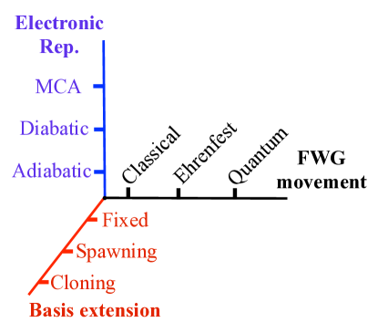
Figure 1: Independent components of FWG-based approaches.

The last aspect mainly concerns the nuclear basis (since the number of electronic states is usually predefined by the problem energy scale). Necessity to increase the number of FWGs stems from differences in complexity of $\Psi(r,R,0)$ and that at later times. Second, several fundamental issues related to the equivalence of different formulations, geometric phase treatment, and energy conservation will be highlighted. Third, we will discuss rigorous extensions of intuitive ideas of the basis extensions (e.g., spawning and cloning) and applying FWG methods for simulating open systems.

Before starting our exposition, we would like to note that even though mixed quantum-classical (MQC) methods^{13, 14, 15} are very popular in the context of the nonadiabatic dynamics, and even though in many popular methods based on Eq. (1) FWGs move classically, we believe that comparison of FWG approaches to those of the MQC methodology can be misleading and we will try to avoid it. We would like to emphasize that FWG methods based on Eq. (1) are fully quantum, even though they have some restrictions on the form of the wavefunction, yet, both electronic $r$ and nuclear $R$ variables are present and completely independent from the time variable. On the other hand, MQC approaches turn the nuclear variables to classical trajectories, which are essentially functions of time. The main advantage of FWG methods with respect to the MQC ones is conceptually straightforward inclusion of all nuclear quantum effects (zero point energy, decoherence, etc.) because it is only a matter of a basis extension to build a nuclear wavefunction capable of describing the necessary effects.

Another popular method to model fully quantum nonadiabatic dynamics is multiconfiguration time-dependent Hartree (MCTDH). ^{16, 17, 18, 19} This method merely reduces the prefactor of the exponential scaling and allows one to consider larger systems than standard grid approaches²⁰. However, MCTDH requires a global parametrization of PESs. One of the main reasons to prefer FWG formulation is avoidance of the PES parametrization and evaluating it on-the-fly.

The rest of this paper is organized as follows. First, we discuss the representations for electron and nuclear basis functions. Second, we give the theoretical background on direct quantum dynamics and discuss the time-dependent variational principle (TDVP) formulation. Then, we expose our extensions of popular methods for increase of the number of nuclear basis functions for variational dynamics. Finally, we present a problem-free approach to open system dynamics using the non-stochastic open system Schrödinger equation (NOSSE).

2 Representations

2.1 Frozen-width Gaussians

One of the first introductions of FWGs to modeling dynamics of nuclear degrees of freedom (DOF) was done by Heller.^{21, 22, 23} Among a few equivalent forms, FWGs in Eq. (1) are usually taken in the coherent states (CS) form

$$g_{k}(\boldsymbol{R}|\boldsymbol{q}_{k}(t),\boldsymbol{p}_{k}(t)) = \prod_{a=1}^{N_{\mathrm{n}}}\left(\frac{\omega_{a}}{\pi}\right)^{1/4}$$ (2)

$$\times \prod_{\alpha=1}^{\mathcal{D}}\mathrm{e}^{-\frac{\omega_{a}}{2}(R_{a\alpha}-q_{ka\alpha})^{2}+ip_{ka\alpha}(R_{a\alpha}-q_{ka\alpha})+ip_{ka\alpha}q_{ka\alpha}/2},$$

where $\omega_{a}$ controls the CS width, $N_{\mathrm{n}}$ is the number of nuclear DOF, and $\mathcal{D}$ is the space dimensionality. This allows one to use the CS algebra, positions of Gaussians centers and their momenta can be replaced by the complex variables $\{\boldsymbol{z}_{k}\}$ according to

$$z_{ka\alpha}(t) = \sqrt{\frac{\omega_{a}}{2}}q_{ka\alpha}(t)+\frac{i}{\sqrt{2\omega_{a}}}p_{ka\alpha}(t).$$ (3)

Using the complex variables $\{\boldsymbol{z}_{k}\}$, CSs read

$$g_{k}(\boldsymbol{R}|\boldsymbol{q}_{k}(t),\boldsymbol{p}_{k}(t)) = g_{k}(\boldsymbol{R}|\boldsymbol{z}_{k}(t),\boldsymbol{z}_{k}^{*}(t))=\prod_{a=1}^{N_{\mathrm{n}}}\left(\frac{\omega_{a}}{\pi}\right)^{1/4}G_{ka}(\vec{R}_{a})$$

$$G_{ka}(\vec{R}_{a}) = \prod_{\alpha=1}^{\mathcal{D}}\mathrm{e}^{-\frac{\omega_{a}}{2}(R_{a\alpha}-\sqrt{\frac{2}{\omega_{a}}}z_{ka\alpha})^{2}+iz_{ka\alpha}\operatorname{Im}(z_{ka\alpha})}.$$ (4)

With these definitions, we have the usual eigenvalue relation for CSs

$$\left[\sqrt{\frac{\omega_{a}}{2}}R_{a\alpha}+\frac{1}{\sqrt{2\omega_{a}}}\frac{\partial}{\partial R_{a\alpha}}\right]g_{k}(\boldsymbol{R}|\boldsymbol{z}_{k}(t),\boldsymbol{z}_{k}^{*}(t)) = z_{ka\alpha}(t)g_{k}(\boldsymbol{R}|\boldsymbol{z}_{k}(t),\boldsymbol{z}_{k}^{*}(t)).$$ (5)

The CS choice for the form of FWGs does not only simplify derivations but also removes some of the numerical issues that plagued other choices.²⁴ One of the main contributions to the success of the CS form is the classical action represented in the phase part $i\sum_{a,\alpha}p_{ka\alpha}q_{ka\alpha}/2$ in Eq. (2). Another FWG choice used in variational Multiconfiguration Gaussian (vMCG) ²⁵ had an extra time-dependent variable that represented this phase and required an additional time-integration to obtain its time-dependence. This extra time-integration was extremely unstable because of highly oscillatory nature of the phase. The classical analogue represented in the CS form captures the majority of the true quantum phase and does not require an additional time-integration.

The nuclear variables $R$ can be either internal DOF (e.g. normal modes) or Cartesian coordinates. In the latter case, optimal $\omega_{a}$’s obtained for individual atoms can be used.²⁶

2.2 Electronic wavefunctions

There are two main choices for the electronic states in Eq. (1), adiabatic and diabatic wavefunctions. In this subsection we summarize pros and cons for both representations and highlight a newly developed moving crude adiabatic (MCA) representation that combines the best properties of the conventional representations and has been introduced recently in the context of the FWG dynamics.²⁷

Adiabatic representation:

The electron-nuclear wavefunction without using a specific FWG nuclear representation can be written as the Born–Huang (BH) expansion

$$\Psi(r,R,t)=\sum_{s}\phi_{s}(r|R)\chi_{s}(R,t),$$ (6)

where $\phi_{s}(r|R)$ electronic eigenstates of the electronic Hamiltonian $H_{e}(r|R)\phi_{s}(r|R)=E_{s}(R)\phi_{s}(r|R)$, and $\chi_{s}(R,t)$ are the nuclear time-dependent wavefunctions. To obtain equations for $\chi_{s}(R,t)$, the total TDSE is projected onto the space of the electronic wavefunctions and the integration over the electronic DOF is done

$$\sum_{s^{\prime}}[(T_{n}+E_{s}(R))\delta_{ss^{\prime}}+\Lambda_{ss^{\prime}}]\chi_{s^{\prime}}(R,t)=i\partial_{t}\chi_{s}(R,t)$$ (7)

Due to the parametric dependence of the adiabatic states on the nuclear DOF, this representation generates nonadiabatic couplings (NACs)

$$\Lambda_{ss^{\prime}} = -\sum_{a\alpha}\frac{1}{2M_{a}}\left\langle\phi_{s}(R)|\frac{\partial^{2}\phi_{s^{\prime}}(R)}{\partial R_{a\alpha}^{2}}\right\rangle_{r}-\sum_{a\alpha}\frac{1}{M_{a}}\left\langle\phi_{s}(R)|\frac{\partial\phi_{s^{\prime}}(R)}{\partial R_{a\alpha}}\right\rangle_{r}\frac{\partial}{\partial R_{a\alpha}}$$ (8)

Among these terms, the diagonal Born–Oppenheimer correction (DBOC),

$$\left\langle\phi_{s}(R)|\frac{\partial^{2}\phi_{s}(R)}{\partial R_{a\alpha}^{2}}\right\rangle_{r}\sim\frac{1}{(E_{s}(R)-E_{s\pm 1}(R))^{2}}$$ (9)

diverges at commonly encountered conical intersections (CIs) ^{28, 29} and makes it impossible to integrate Eq. (7). ³⁰

An additional problem arising due to CIs is appearance of nontrivial Berry or geometric phase (GP) in the electronic wavefunctions of states involved in the CIs. ^{31, 32, 33} This phase makes the electronic wavefunction change their signs if one evolves them continuously around the CI seam. Thus, the electronic wavefunctions of states experiencing the CI are double-valued with respect to the nuclear variables $R$. This extra feature profoundly affects nuclear dynamics, both for cases when the system evolves on a single PES involved in the CI and when the system participates in the interstate transitions through the CI.³⁴ Ignoring the GP can lead to completely inadequate nuclear dynamics.^{35, 36, 37, 38, 39, 40, 41} Accounting for the GP can be done by introducing a resolution of the identity $1=\exp(i\theta(R))\exp(-i\theta(R))$ to the BH expansion (Eq. (6)), where $\exp(i\theta(R))$ is a double-valued function that compensates double-valuedness of both electronic and nuclear wavefunctions.⁴² However, constructing $\theta(R)$ for the on-the-fly approaches using FWGs can be challenging because $\theta(R)$ should encode global topological properties of the CI seam positions.

One can see that the origin of all the problems stems from the $R$-dependence of electronic wavefunctions $\phi_{s}(r|R)$ and the nuclear kinetic energy operator terms $\Lambda_{ss^{\prime}}$ originating from this dependence. On the other hand, the $R$-dependence in $\phi_{s}(r|R)$ allows one to have a compact electronic representation because calculating the electronic states in a single point (crude adiabatic representation) would require a long expansion for the total wavefunction. A natural solution is to minimize the negative impact of the nuclear dependence in the electronic wavefunctions, and it leads to a so-called diabatic representation.

Diabatic representation:

Changing from adiabatic to diabatic representation removes the NACs and the GP and thus resolves both problems ^{12, 43, 11, 44}

$$\Psi(r,R,t)=\sum_{s}\phi_{s}(r)\tilde{\chi}_{s}(R,t),$$ (10)

where

$$\phi_{s}(r)=\sum_{s^{\prime}}U_{ss^{\prime}}(R)\phi_{s^{\prime}}(r|R).$$ (11)

This leads to the analogous equations for nuclear wavefunctions

$$\sum_{s^{\prime}}[T_{N}\delta_{ss^{\prime}}+V_{ss^{\prime}}]\tilde{\chi}_{s^{\prime}}(R,t)=i\partial_{t}\tilde{\chi}_{s}(R,t),$$ (12)

where $V_{ss^{\prime}}=\left\langle\phi_{s}|H_{e}|\phi_{s^{\prime}}\right\rangle_{r}$.

Unfortunately, the diabatization transformation (Eq. (11)) is generally exact only in a complete set of electronic states, and is approximate otherwise. In the latter case, the transformation in Eq. (11) is known as quasi-diabatization. Quasi-diabatizations are employed to remove the largest, singular at CIs, part of the NACs. Quasi-diabatization technics for on-the-fly (direct) dynamics include regularized diabatization, ^{45, 25, 12} local integration of the NACs, ⁴³ or time-dependent quasi-diabatization. ⁴⁴ While the remaining part of the NACs is considered to be negligible, the error introduced is difficult to control. Furthermore, for direct dynamics, such a quasi-diabatization can only be done in some regions of the nuclear space (e.g. at a known CI position or at FWG centers), which can leave singularities in other regions of the nuclear space. The recently introduced diabatic Gaussians on adiabatic states (DGAS) basis solves this problem by applying a local diabatization at each FWG center. ⁴⁴

MCA representation:

All problems of the global diabatic and adiabatic representations are avoided by simply replacing the dependence of the electronic states on the nuclear DOF by their dependence on the FWGs’ centers, $q_{k}(t)$,

$$\Psi(r,R,t)=\sum_{k,s}C_{ks}(t)g_{k}(R|q_{k}(t),p_{k}(t))\phi_{s}(r|q_{k}(t)).$$ (13)

The resulting electronic states $\phi_{s}(r|q_{k}(t))$ are adiabatic only at $\boldsymbol{q}_{k}$ but used for any other nuclear geometries and are commonly referred to as crude adiabatic states. ^{46, 47} Since these crude adiabatic states are attached to the moving Gaussians, we refer to the expansion in Eq. (13) as the moving crude adiabatic (MCA) representation, ²⁷ also known as time-dependent diabatic basis. ¹¹ In fact, the MCA representation is a rigorous diabatic representation because the electronic wavefunctions do not have any $R$-dependence. It becomes very important to distinguish the nuclear variables $R$ and the FWGs’ centers $q_{k}(t)$. As $\phi_{s}(r|q_{k}(t))$ do not depend on nuclear DOF, the nuclear kinetic energy operator has no effect on the MCA states, so that NACs are exactly zero.

It is also possible to show a precise mechanism of the MCA solution of the GP problem. The MCA representation can be obtained starting from an exact complete diabatic representation $\{\phi_{s}\}$ by applying rotations $\boldsymbol{Q}(q_{k})$ to a set of adiabatic states at the Gaussians’ centers

$${H}_{\mathrm{e}}[\boldsymbol{q}_{k}]\sum_{u}\left|\phi_{u}\right\rangle Q_{us}(q_{k}) = {H}_{\mathrm{e}}[\boldsymbol{q}_{k}]\left|\phi_{s}(q_{k})\right\rangle=E_{s}(\boldsymbol{q}_{k})\left|\phi_{s}(q_{k})\right\rangle.$$ (14)

Applying this transformation to the total wavefunction in the diabatic representation gives the MCA representation

$$\left|\Psi\right\rangle = \sum_{ku}\tilde{C}_{ku}\left|g_{k}\right\rangle\left|\phi_{u}\right\rangle$$ (15)

$$= \sum_{ks}\left(\sum_{u}\tilde{C}_{ku}Q_{us}(q_{k})\right)\left(\sum_{v}\left|\phi_{v}\right\rangle Q_{vs}(q_{k})\right)\left|g_{k}\right\rangle$$

$$= \sum_{ks}{C}_{ks}(q_{k})\left|g_{k}\right\rangle\left|\phi_{s}(q_{k})\right\rangle,$$

where we used orthogonality of the rotation matrix $\boldsymbol{Q}(q_{k}){\boldsymbol{Q}(q_{k})}^{T}=\boldsymbol{1}$, while the last equality is Eq. (13). For CIs, $\boldsymbol{Q}(q_{k})$ is double-valued due to appearance of GP along any path followed by $\boldsymbol{q}_{k}$ encircling the CI. Thus, the MCA states are double-valued as functions of $\boldsymbol{q}_{k}$. Equation (15) shows that the coefficients ${C}_{ks}(q_{k})$ are also double-valued in the parameter space and compensate for the double-valuedness of the MCA states. By construction, the MCA representation provides double-valuedness to nuclear wavepackets $\sum_{k}{C}_{ks}(q_{k})\left|g_{k}\right\rangle$ and the GP is naturally included in the approach.

2.3 Multi-set and single-set

Upon deciding on the form of FWGs and the electronic state representation, there are still two choices left in combining the electronic and nuclear functions in linear combination of Eq. (1). The key difference between these choices is whether FWG positions and momenta depend on the electronic state multiplying FWGs, multi-set

$$\Psi(r,R,t)=\sum_{k,s}C_{ks}(t)g_{k}(R|q_{k}^{(s)}(t),p_{k}^{(s)}(t))\tilde{\phi}_{s}(r)$$ (16)

or not, single-set

$$\Psi(r,R,t)=\sum_{k,s}C_{ks}(t)g_{k}(R|q_{k}(t),p_{k}(t))\tilde{\phi}_{s}(r),$$ (17)

where $\tilde{\phi}_{s}(r)$ can be electronic states of any representation discussed above. Both sets converge to the same limit, but they start from different points.

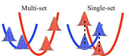
Figure 2: Illustration of multi-set and single-set FWGs.

Multi-set is more adapted toward nuclear dynamics that is very different on different electronic states (Fig. 2 left), an alternative form of Eq. (16) illustrating this view is

$$\Psi(r,R,t)=\sum_{s}\tilde{\phi}_{s}(r)\left[\sum_{k}C_{ks}(t)g_{k}(R|q_{k}^{(s)}(t),p_{k}^{(s)}(t))\right],$$ (18)

here, every electronic wavefunction has its own linear combination of FWGs. In contrast, the starting point of the single-set is similar dynamics of each FWG on multiple electronic states (Fig. 2 right), or alternatively, it is a motion of a stack of FWGs with the same positions and momenta but different amplitudes. Therefore, each FWG in single-set can be thought as multiplied by its own time-dependent superposition of electronic states

$$\Psi(r,R,t)=\sum_{k}g_{k}(R|q_{k}(t),p_{k}(t))\left[\sum_{s}C_{ks}(t)\tilde{\phi}_{s}(r)\right].$$ (19)

Both sets have been used before, the main advantage of multi-set is perfect description of nuclear decoherence effects while making it difficult for FWGs on different electronic states to interact because of vanishing nuclear space overlap. The opposite is true for the single-set where the main advantage is for replicas of a FWG in the same stack to exchange the population readily because of the perfect overlap. On the other hand, description of nuclear decoherence in the single-set requires increasing numbers of FWGs.

3 Equations of motion

A general approach to obtain differential equations for time-dependence of FWG parameters involves application of the TDVP. In this section we will illustrate caveats related to various forms of the TDVP, its partial application, and energy and norm conservation problems.

3.1 Various forms of the time-dependent variational principle

Three different forms of the TDVP can be found, first, the Dirac-Frenkel (DF) TDVP^{48, 49}

$$\left\langle\delta\Psi|H-i\partial_{t}|\Psi\right\rangle = 0,$$ (20)

which is based on imposing orthogonality of all possible variations allowed by the parametrization, $\delta\Psi$, to the error vector in the TDSE due to the wavefunction parametrization, $\left|(H-i\partial_{t})\Psi\right\rangle$. This orthogonality ensures the optimal choice of parameters’ time-dependence, since the residual error cannot be reduced further by any variation of the parameters. Second, the McLachlan TDVP,⁵⁰ which is rooted in minimization of the error vector norm $||(H-i\partial_{t})\left|\Psi\right\rangle||$, results in⁵¹

$$\operatorname{Im}\left\langle\delta\Psi|H-i\partial_{t}|\Psi\right\rangle = 0.$$ (21)

Third, the stationary action principle, here the quantum action defined as⁵¹

$$\mathcal{S}[\Psi]=\int_{t_{0}}^{t_{1}}\left\langle\Psi|H-i\partial_{t}|\Psi\right\rangle dt$$ (22)

is varied with respect to wavefunction parameters’ as functions of time. The condition $\delta\mathcal{S}[\Psi]=0$ is equivalent to the equation⁵¹

$$\operatorname{Re}\left\langle\delta\Psi|H-i\partial_{t}|\Psi\right\rangle = 0.$$ (23)

Yet, all these versions of the TDVP are found to give the same equations of motion (EOM) if the wavefunction parametrization is analytic in the complex variable sense (function $f$ of complex variable $z$ is analytic if $\partial f(z)/\partial z^{*}=0$).⁵¹ Functions based on CSs are generally non-analytic because of $z_{ka\alpha}^{*}$ dependencies in CSs (Eq. (4)). Non-analyticity of electron-nuclear basis products can be decomposed in two components originating from nuclear and electronic parts

$$\left|\frac{\partial(g_{k}\phi_{s})}{\partial z_{ka\alpha}^{*}}\right\rangle = \left|\frac{\partial g_{k}}{\partial z_{ka\alpha}^{*}}\phi_{s}\right\rangle+\left|g_{k}\frac{\partial\phi_{s}}{\partial z_{ka\alpha}^{*}}\right\rangle.$$ (24)

The global adiabatic and diabatic representations do not have the second electronic term in Eq. (24). For these representations even the non-analyticity stemming from individual CSs do not affect the EOM because terms corresponding to $z_{ka\alpha}^{*}$ derivatives vanish. Thus, all three forms of the TDVP give the same EOM for the global adiabatic and diabatic representations. One of the most well-known approaches derived in the diabatic representation using the DF TDVP is the vMCG method. ¹²

Similar to the other representations, for MCA, non-analyticity of individual CSs (the first term in Eq. (24)) does not contribute to EOM, however, the electronic wavefunctions depend on $q_{ka}\sim z_{ka\alpha}+z_{ka\alpha}^{*}$, and therefore, due to this non-analyticity all TDVP forms give different EOM for the MCA representation. Among the three TDVP versions, only the stationary action principle is proven to lead to EOM necessarily conserving the system energy,⁵² and thus, we illustrate the MCA EOM based on this principle.

We will use the MCA representation with the single-set expansion, $\left|\Psi\right\rangle=\sum_{ks}C_{ks}\left|\varphi_{ks}\right\rangle$ where the electron-nuclear basis functions $\{\varphi_{ks}\}$ are

$$\varphi_{ks}(\boldsymbol{R},\boldsymbol{r}|\boldsymbol{z}_{k}(t),\boldsymbol{z}_{k}^{*}(t)) = g_{k}(\boldsymbol{R}|\boldsymbol{z}_{k}(t),\boldsymbol{z}_{k}^{*}(t))\phi_{s}(\boldsymbol{r}|\boldsymbol{z}_{k}(t),\boldsymbol{z}_{k}^{*}(t)).$$ (25)

In order to simplify equations we will use the short-hand notation, $\phi_{s}(\boldsymbol{r}|\boldsymbol{z}_{k}(t),\boldsymbol{z}_{k}^{*}(t))\equiv\left|\phi_{s}^{k}\right\rangle$, and will omit the time and nuclear coordinates. Using Eq. (23) we obtain the system of coupled equations

$$\partial_{t}{\boldsymbol{C}} = \boldsymbol{S}^{-1}(-i\boldsymbol{H}-\boldsymbol{\gamma})\boldsymbol{C},$$ (26)

$$\boldsymbol{B}\partial_{t}{\boldsymbol{z}}+\boldsymbol{A}\partial_{t}{\boldsymbol{z}}^{*} = \boldsymbol{Y}+\overline{\boldsymbol{Y}},$$ (27)

where matrices and vectors are defined as

$$S_{kl,ss^{\prime}} = \left\langle\varphi_{ks}|\varphi_{ls^{\prime}}\right\rangle,$$ (28)

$$H_{kl,ss^{\prime}} = \left\langle\varphi_{ks}\left|{H}\right|\varphi_{ls^{\prime}}\right\rangle,$$ (29)

$$\gamma_{kl,ss^{\prime}} = \left\langle\varphi_{ks}|\partial_{t}\varphi_{ls^{\prime}}\right\rangle,$$ (30)

$$Y_{ka\alpha} = i\sum_{lss^{\prime}}C_{ks}^{*}\left\langle\frac{\partial\varphi_{ks}}{\partial z_{ka\alpha}}\left|{1}-{\mathcal{P}}\right|{H}\varphi_{ls^{\prime}}\right\rangle C_{ls^{\prime}},$$ (31)

$$\overline{Y}_{ka\alpha} = i\sum_{lss^{\prime}}C_{ls^{\prime}}^{*}\left\langle{H}\varphi_{ls^{\prime}}\left|{1}-{\mathcal{P}}\right|\frac{\partial\varphi_{ks}}{\partial z_{ka\alpha}^{*}}\right\rangle C_{ks},$$ (32)

$$A_{kl,ab,\alpha\beta} = \sum_{ss^{\prime}}\Bigg{[}C_{ls^{\prime}}^{*}\left\langle\frac{\partial\varphi_{ls^{\prime}}}{\partial z_{lb\beta}}\left|{1}-{\mathcal{P}}\right|\frac{\partial\varphi_{ks}}{\partial z_{ka\alpha}^{*}}\right\rangle C_{ks}$$ (33)

$$-C_{ks}^{*}\left\langle\frac{\partial\varphi_{ks}}{\partial z_{ka\alpha}}\left|{1}-{\mathcal{P}}\right|\frac{\partial\varphi_{ls^{\prime}}}{\partial z_{lb\beta}^{*}}\right\rangle C_{ls^{\prime}}\Bigg{]},$$

$$B_{kl,ab,\alpha\beta} = \sum_{ss^{\prime}}\Bigg{[}C_{ls^{\prime}}^{*}\left\langle\frac{\partial\varphi_{ls^{\prime}}}{\partial z_{lb\beta}^{*}}\left|{1}-{\mathcal{P}}\right|\frac{\partial\varphi_{ks}}{\partial z_{ka\alpha}^{*}}\right\rangle C_{ks}$$ (34)

$$-C_{ks}^{*}\left\langle\frac{\partial\varphi_{ks}}{\partial z_{ka\alpha}}\left|{1}-{\mathcal{P}}\right|\frac{\partial\varphi_{ls^{\prime}}}{\partial z_{lb\beta}}\right\rangle C_{ls^{\prime}}\Bigg{]}.$$

Equations (31-34) involve the projector on the non-orthogonal basis

$${\mathcal{P}} = \sum_{kl,ss^{\prime}}\left|\varphi_{ks}\right\rangle[\boldsymbol{S}^{-1}]_{kl,ss^{\prime}}\left\langle\varphi_{ls^{\prime}}\right|.$$ (35)

Here, it is easy to see that the non-analyticity from the CSs derivatives vanish, the corresponding terms appearing in Equations (31-34) will contain projections of the derivatives

$$({1}-{\mathcal{P}})\left|\frac{\partial g_{k}}{\partial z_{ka\alpha}^{*}}\phi_{s}^{k}\right\rangle = -({1}-{\mathcal{P}})\frac{z_{ka\alpha}}{2}\left|\varphi_{ks}\right\rangle\equiv 0,$$ (36)

where we used the CS definition to obtain the explicit form of the derivatives. These derivative terms vanish because projector ${\mathcal{P}}$ is equivalent to the identity operator for the basis $\{\varphi_{ks}\}$.

Equation (27) can be solved by combining it with its complex conjugate to the system of equations

$$\begin{pmatrix}\boldsymbol{B}&\boldsymbol{A}\\ \boldsymbol{A}^{\dagger}&-\boldsymbol{B}^{T}\end{pmatrix}\begin{pmatrix}\partial_{t}{\boldsymbol{z}}\\ \partial_{t}{\boldsymbol{z}}^{*}\end{pmatrix} = \begin{pmatrix}{\boldsymbol{Y}}+\overline{\boldsymbol{Y}}\\ -{\boldsymbol{Y}}^{*}-\overline{\boldsymbol{Y}}^{*}\end{pmatrix},$$ (37)

and then solving the system by block matrix inversion

$$\begin{pmatrix}\partial_{t}{\boldsymbol{z}}\\ \partial_{t}{\boldsymbol{z}}^{*}\end{pmatrix} = \begin{pmatrix}\boldsymbol{\beta}&\boldsymbol{\alpha}\\ \boldsymbol{\alpha}^{\dagger}&-\boldsymbol{\beta}^{T}\end{pmatrix}\begin{pmatrix}{\boldsymbol{Y}}+\overline{\boldsymbol{Y}}\\ -{\boldsymbol{Y}}^{*}-\overline{\boldsymbol{Y}}^{*}\end{pmatrix},$$ (38)

where

$$\boldsymbol{\beta} = [\boldsymbol{B}+\boldsymbol{A}(\boldsymbol{B}^{T})^{-1}\boldsymbol{A}^{\dagger}]^{-1},$$ (39)

$$\boldsymbol{\alpha} = \boldsymbol{B}^{-1}\boldsymbol{A}\boldsymbol{\beta}^{T}=\boldsymbol{\beta}\boldsymbol{A}(\boldsymbol{B}^{T})^{-1}.$$ (40)

The obtained equations is somewhat similar to those in other methods using FWGs and the TDVP such as vMCG and G-MCTDH, but there are clear differences stemming from the MCA representation.

3.2 Conservation of norm and energy

Equation (26) have the property that the norm of the wavefunction is conserved by construction

$$\partial_{t}\left\langle\Psi|\Psi\right\rangle = 2\operatorname{Re}\left\langle\Psi|\partial_{t}\Psi\right\rangle$$ (41)

$$= 2\operatorname{Re}\left({\boldsymbol{C}}^{\dagger}\boldsymbol{S}\partial_{t}{\boldsymbol{C}}+\boldsymbol{C}^{\dagger}{\boldsymbol{\gamma}}\boldsymbol{C}\right)$$

$$= 2\operatorname{Im}\left({\boldsymbol{C}}^{\dagger}\boldsymbol{H}\boldsymbol{C}\right)=0,$$

where we used hermiticity of $\boldsymbol{H}$. The system energy is also conserved by construction for a time-independent Hamiltonian, as it can be verified by using Eqs. (26,31,32,38):

$$\partial_{t}E = 2\operatorname{Re}\left\langle\Psi\left|{H}\right|\partial_{t}\Psi\right\rangle$$ (42)

$$= 2\operatorname{Re}\left[i\overline{\boldsymbol{Y}}^{\dagger}\partial_{t}{\boldsymbol{z}}-i\boldsymbol{Y}^{T}\partial_{t}{\boldsymbol{z}}^{*}\right]$$

$$= 2\operatorname{Im}\left[\begin{pmatrix}\overline{\boldsymbol{Y}}\\ -\boldsymbol{Y}^{*}\end{pmatrix}^{\dagger}\begin{pmatrix}\boldsymbol{\beta}&\boldsymbol{\alpha}\\ \boldsymbol{\alpha}^{\dagger}&-\boldsymbol{\beta}^{T}\end{pmatrix}\begin{pmatrix}\boldsymbol{Y}+\overline{\boldsymbol{Y}}\\ -\boldsymbol{Y}^{*}-\overline{\boldsymbol{Y}}^{*}\end{pmatrix}\right],$$

$$= -2\operatorname{Im}\left[\begin{pmatrix}\overline{\boldsymbol{Y}}^{*}\\ -\boldsymbol{Y}\end{pmatrix}^{T}\begin{pmatrix}\boldsymbol{\alpha}&\boldsymbol{\beta}\\ -\boldsymbol{\beta}^{T}&\boldsymbol{\alpha}^{\dagger}\end{pmatrix}\begin{pmatrix}\overline{\boldsymbol{Y}}^{*}\\ -\boldsymbol{Y}\end{pmatrix}\right]=0.$$

In the last two equalities we used that $\boldsymbol{\beta}$ and $\boldsymbol{\alpha}$ are hermitian and antisymmetric, respectively.

3.3 Classically moving Gaussians

The TDVP equations for $z$ and $z^{*}$ (or effectively $p$ and $q$) are the most time-consuming because of the dimensionality of the involved matrices. One can apply the TDVP to FWG expansions to obtain EOM only for the amplitudes $C_{ks}$, while EOM for the FWG evolution can be chosen to be classical (or Ehrenfest). This reduced approach still gives rise to quantum formalism because both electronic and nuclear wavefunctions are present. It has been used in the multiconfiguration Ehrenfest (MCE) method of Shalashilin ^{24, 11} (single-set basis) and the ab inito multiple spawning (AIMS) method of Martinez ^{53, 54, 10} (multi-set basis). These approaches have the advantage that each FWG propagation can be done independently (in parallel) from others, so that, later, the information on individual trajectories can be used for solving Eq. (26) and obtaining the amplitudes $C_{ks}$.

However, using classical EOM for FWGs affects two properties, which are intertwined in this case: the convergence with respect to the number of nuclear basis functions and the energy conservation. Classical motion of FWGs increases requirements for the number of basis functions in general. It is related to quantum forces appearing in the full TDVP formalism that make FWG movement more optimal.²⁵ Also, formalisms using classical FWG motion do not conserve the total energy.⁵⁵ The energy conservation problem can be reduced by increasing the basis set because at the complete basis set limit the motion of FWGs does not affect the formalism. On the other hand, the energy conservation becomes especially problematic when two or more FWGs overlap significantly in the course of their dynamics. The energy conserving FWG motion is predicted by the full TDVP, whereas deviations from it based on classical dynamics can be considered as interference of an external force. Clearly, the total energy is not generally conserved in this case. In contrast, if FWGs do not overlap significantly, TDVP FWG motion reduces to their classical motion in accordance with the Ehrenfest theorem, and the energy is conserved. The latter scenario is more probable for general, large dimensional systems, where nuclear decoherence is usually fast. Nevertheless, due to advantages provided by independent FWG evolution schemes, the work on developing a FWG-based method with uncoupled trajectories that would conserve the energy is highly desirable.

3.4 Integral evaluation

Solving Eqs. (26) and (37) require matrix elements involving integration with respect to both electronic and nuclear coordinates. For the global adiabatic and diabatic representations, the TDVP is effectively applied to Eqs. (6) and (10) because the electronic states in these representations do not contain parameters subject to the optimization. In solving these equations, the electron-nuclear integration is done in two steps, first, the electronic variables are integrated in electronic structure programs, and then nuclear dependent quantities are integrated with FWGs. In relation to the nuclear integration, the diabatic models are convenient because all integrals with nuclear FWGs are analytic due to polynomic form of the $V_{ss^{\prime}}(R)$ functions. The adiabatic representation is more challenging due to less smooth behavior of PESs and divergencies of NACs near CI seams. Furthermore, adiabatic and diabatic states dependence on nuclear coordinates is generally not known so that one must resort to local approximate models for the nuclear integration. Locality of FWGs helps for introducing approximations into matrix elements arising in solving Eq. (7). Let us consider matrix element $\left\langle g_{k}(q_{k})|A(R)|g_{l}(q_{l})\right\rangle_{R}$ appearing in computational schemes based on Eq. (7) and expanding $\chi_{s}(R,t)$ as a linear combination of FWGs, here, $A(R)$ is either PES or NAC. Note, that a product of two FWGs, $g_{k}(R|q_{k})$ and $g_{l}(R|q_{l})$, is again a FWG centered in between the centers of the two FWGs, $q_{c}=(q_{k}+q_{l})/2$, this relation is also known as the Gaussian Product Rule. A typical estimation of the integral of interest involves a Taylor series expansion of $A(R)$ at $q_{c}$¹⁰

$$\left\langle g_{k}(q_{k})|A(R)|g_{l}(q_{l})\right\rangle_{R} \approx A(q_{c})\left\langle g_{k}(q_{k})|g_{l}(q_{l})\right\rangle_{R}+\sum_{a\alpha}\frac{\partial A(R)}{\partial R_{a\alpha}}\Bigg{|}_{R=q_{c}}$$ (43)

$$\times\left\langle g_{k}(q_{k})|(R_{a\alpha}-q_{c,a\alpha})|g_{l}(q_{l})\right\rangle_{R}+\frac{1}{2}\sum_{a\alpha,b\beta}\frac{\partial^{2}A(R)}{\partial R_{a\alpha}\partial R_{b\beta}}\Bigg{|}_{R=q_{c}}$$

$$\times\left\langle g_{k}(q_{k})|(R_{a\alpha}-q_{c,a\alpha})(R_{b\beta}-q_{c,b\beta})|g_{l}(q_{l})\right\rangle_{R},$$

where the integrals of FWGs with polynoms of $R$ (Gaussian moments) are analytical, but calculating the $A(R)$ derivatives increases the computational cost.

One of the greatest advantages of the MCA representation is that typical approximations for PESs and NACs can be avoided completely, even though the MCA representation comes from solving the electronic structure problem like the adiabatic representation. The key element for avoiding approximations is a different partitioning of the total molecular Hamiltonian, $H=h_{e}(\boldsymbol{r})+h_{n}(\boldsymbol{R})+V_{en}(|\boldsymbol{r}-\boldsymbol{R}|)$, here by grouping all electron and nuclear variables in $h_{e}(\boldsymbol{r})$ and $h_{n}(\boldsymbol{R})$ we expose the only electron-nuclear Coulomb coupling term, $V_{en}$. This partitioning does not even introduce PESs as intermediate quantities. Instead, matrix elements such as in Eq. (29) can be evaluated numerically exactly

$$\left\langle\varphi_{ks}\left|{H}\right|\varphi_{ls^{\prime}}\right\rangle = \left\langle\phi_{ks}\left|{h}_{e}\right|\phi_{ls^{\prime}}\right\rangle_{r}\left\langle g_{k}|g_{l}\right\rangle_{R}+\left\langle g_{k}\left|{h}_{n}\right|g_{l}\right\rangle_{R}\left\langle\phi_{s}|\phi_{s^{\prime}}\right\rangle_{r}+\left\langle\varphi_{ks}\left|{V}_{en}\right|\varphi_{ls^{\prime}}\right\rangle.$$

Note that both electronic and nuclear basis functions are FWGs at a single particle level, therefore, effective Gaussian integration techniques⁵⁶ can be used. The other matrix elements (Eqs. (28)-(34)) also benefit from the new Hamiltonian partitioning and the MCA factorization of electronic and nuclear variables.⁵⁷ Therefore, the MCA representation provides a framework that is free of any approximation other than finite number of the basis functions.

4 Nuclear basis set extensions

One of the main limitations of the FWG based schemes is a finite number of basis functions. Usually, the system wavefunction increases its complexity with time. Any finite number of basis functions will not be able to keep up with this increase. An intuitive solution is to devise an algorithm that cautiously increases the number of basis functions along the course of dynamics. Depending on a particular form of the used set, multi- or single-set, there were two ideas put forward: spawning⁵³ and cloning⁵⁸ (Fig. 3).

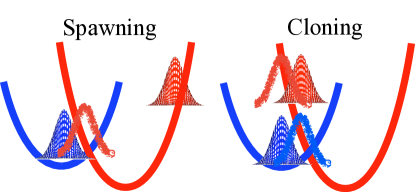
Figure 3: Illustration of spawning and cloning basis set extensions.

In spawning for multi-set, the main problem of a finite basis is that dynamics of FWGs on different electronic states are governed by different forces. This leads to quick nuclear decoherence and thus decay of nuclear overlaps (in Eq. (28)) between FWGs on different surfaces. Without the overlap the transition of the population between electronic states is impossible, therefore, even if a FWG approaches a region of strong coupling (Fig. 2 left) it cannot pass any population unless there is an overlapping FWG on the other electronic state. To correct for this inadequacy of a finite basis set expansion, the spawning procedure would create a new FWG with an initial zero amplitude so that needed population transfer can occur (Fig. 3 left).

In the single-set basis, the population transfer can always occur due to the perfect overlap between replicas of any FWGs in the same stack (Fig. 2 right). The main problem of the single-set finite basis representation is “over-coherence”. In other words, a FWG stack always moves influenced by an averaged electronic state. To correct for “over-coherence”, it is sensible to split stacks of FWGs when individual components experience forces which are very different. To maintain the single-set structure, the split FWGs obtain empty (zero amplitude) counterparts immediately after the split (Fig. 3 right).

The original implementations of spawning and cloning techniques were done for classically moving FWG schemes (AIMS and MCE) and were treating each nuclear FWG separately disregarding that they are part of the total wavefunction. The aim of this section is to illustrate rigorous extensions of these ideas to fully quantum TDVP based formalisms. Here, we will use the diabatic electronic states, but extensions to different electronic representations are possible.

Perturbative spawning (PS):

Two main questions that the PS algorithm addresses is when and where to spawn? To illustrate how these questions are addressed it is instructive to consider two sets of nuclear FWGs representing diabatic nuclear wavefunctions (Eq. (10)) for a two-electronic-state problem (e.g. Fig. 3 left). Two conditions need to be satisfied for the PS algorithm to start a spawning sequence: 1) nuclear components of one or both electronic states reached a nuclear configuration region where there is a significant population flow between the electronic states, and 2) the current FWG representation does not represent this flow adequately. To assess these two conditions we use perturbative estimates of population transfer between the electronic states, where diabatic interstate couplings are treated as a perturbation for a zero-order Hamiltonian corresponding to diabatic states. The diabatic representation is particularly amenable to the formulation of such estimates in the second order of time-dependent perturbation theory because general quadratic forms can be used for diabatic potentials and couplings.^{59, 60} To obtain a numerical estimate for the first condition we evaluate the electronic state population change due to a transition from state $s$ that has a nuclear wavefunction $\chi_{s}(R,t)=\sum_{k}C_{ks}(t)g_{k}(R|q_{k}^{(s)}(t),p_{k}^{(s)}(t))$ to state $s^{\prime}$ assuming that the receiving state ($s^{\prime}$) can use the complete basis set of harmonic oscillator eigenstates. This population change will be denoted as $P^{(c)}_{s\rightarrow s^{\prime}}$. For the second condition, we obtain the same population change but only with a restriction that $s^{\prime}$ can only accept the population from $s$ onto the limited basis that it has, $P^{(l)}_{s\rightarrow s^{\prime}}$. Comparing these two estimates, $|P^{(l)}_{s\rightarrow s^{\prime}}-P^{(c)}_{s\rightarrow s^{\prime}}|>\epsilon$ allows us to make a conclusion whether the nuclear basis on $s^{\prime}$ has enough FWGs to facilitate the population transfer. If the answer is negative, and spawning is needed, a new FWG is created by optimizing its position and momentum to minimize the difference between $P^{(l)}_{s\rightarrow s^{\prime}}$ and $P^{(c)}_{s\rightarrow s^{\prime}}$.⁶¹

The PS procedure is similar to a perturbative extension of configuration interaction space in electronic structure methods such as the B_K method.^{62, 63} The PS approach can also be generalized to locally quadratic diabatization formalisms used in vMCG. Some form of the diabatic representation is necessary for this spawning technique because a local quadratic representation is needed for analytical summation over vibrational states to evaluate $P^{(c)}_{s\rightarrow s^{\prime}}$ quantities.

Quantum cloning (QC):

To illustrate the QC procedure for the total wavefunction, let us consider a case in Fig. 3 (right) with single-set FWGs on two diabatic electronic states. EOM for stacked pairs are obtained using the action extremum corresponding to Eq. (23), which results in the following variations for positions and momenta of FWGs encoded in $z_{k}$’s

$$\operatorname{Re}\Bigg{\langle}\delta z_{k}\frac{\partial\Psi}{\partial z_{k}}\Bigg{|}H-i\partial_{t}\Bigg{|}\Psi\Bigg{\rangle}=0,~{}\forall k.$$ (45)

However, if one allows any pair of stacked FWGs to evolve as components of multi-set, their evolution will be different because all FWG replicas experience different forces on different electronic states. In other words, at any moment in time if one considers the total electron nuclear wavefunction with all CSs pairs within $N_{G}-1$ single-set and the $k^{\rm th}$ pair to be multi-set

$$\Psi_{k}(r,R,t)=\sum_{s}\phi_{s}(r)\left[C_{ks}g_{k}(R|q_{k}^{(s)}(t),p_{k}^{(s)}(t))+\sum_{k^{\prime}\neq k}C_{k^{\prime}s}g_{k^{\prime}}(R|q_{k^{\prime}}(t),p_{k^{\prime}}(t))\right],$$ (46)

then because this relaxation (or addition of parameters) came suddenly the variations with respect to individual electronic state $z_{k}^{(s)}$ will be non-zero

$$\operatorname{Re}\left[\sum_{s}\delta z_{k}^{(s)}\Bigg{\langle}\frac{\partial\Psi_{k}}{\partial z_{k}^{(s)}}\Bigg{|}H-i\partial_{t}\Bigg{|}\Psi_{k}\Bigg{\rangle}\right]\neq 0.$$ (47)

This variation contains arbitrary functions $\delta z_{k}^{(s)}(t)$, which can be removed to assess the effect of the $k^{\rm th}$ pair split. Naturally, the criterion for splitting the $k^{\rm th}$ pair becomes the sum over the electronic states

$$\sum_{s}\left|\operatorname{Re}\Bigg{\langle}\frac{\partial\Psi_{k}}{\partial z_{k}^{(s)}}\Bigg{|}H-i\partial_{t}\Bigg{|}\Psi_{k}\Bigg{\rangle}\right|>\epsilon,$$ (48)

which can be thought as “decoherence strain”. This criterion can be applied for any of the $N_{G}$ single-set pairs at any moment in time. It reduces to an intuitive criterion suggested before for an individual pair of CSs and accounts for situations when other CS pairs of the full electron-nuclear wavefunction may reduce the necessity of splitting a particular pair.

Clear advantage of the QC algorithm compare to the PT scheme is use of quantities that are already available in regular TDVP algorithms without basis set extensions. This makes QC easily applicable not only in the diabatic representation but also in the adiabatic and MCA representations.

5 Dynamics of open systems

To extend the domain of applicability for TDVP-based FWG methods to even larger systems, one can try to generalize these methods to open systems. Here, by an open system we will understand a molecular subsystem that is capable of energy but not matter exchange with its environment. For example, such systems can be chromophores of photoactive proteins coupled to a protein environment (e.g. rhodopsin) ^{64, 65} or a molecule interacting with incoherent light. ^{66, 67} Due to a large number of environmental DOF, only subsystem dynamics is considered explicitly while environmental DOF are integrated out.^{68, 69} This leads to a formalism where the subsystem density (${\rho}$) is the main dynamical quantity following the quantum master equation (QME), $\partial_{t}{\rho}=\mathcal{L}[{\rho}]$ with $\mathcal{L}$ as a super-operator modifying the subsystem density. If the subsystem is uncoupled from the environment, QME becomes the Liouville-von Neumann equation, $\mathcal{L}[{\rho}(t)]=-i[{H},{\rho}(t)]$, then the subsystem is considered to be closed and energy must be conserved.

Combining the McLachlan TDVP with QME is equivalent to minimizing the error $||\partial_{t}{\rho}-\mathcal{L}[{\rho}]||$ where $||\cdot||$ is the Frobenius (or Hilbert-Schmidt) norm, which results in the following stationary condition ⁷⁰

$$\mathrm{tr}\{\delta{\rho}^{\dagger}(\partial_{t}{\rho}-\mathcal{L}[{\rho}])\} = 0.$$ (49)

Solving Eq. (49) using a finite set of moving FWGs leads to two unphysical features for the density matrix evolution: 1) the density matrix trace (the subsystem population) is not conserved for an open system, ^{71, 70, 72} and 2) the energy is not conserved in the closed system limit. ^{50, 22, 70, 72} The latter leads to an unphysical energy flow channel in the corresponding open system and results in wrong dynamics of the subsystem.

Violation of energy conservation for the closed system is not related to non-analyticity of the density matrix ansatz since this violation also occurs for analytic parameterizations as well.^{70, 72} For the sake of simplicity, we will consider an analytic parametrization of the density matrix (e.g. Bargmann states⁷³ for the nuclear basis in the diabatic representation). The problem of energy flow appear as a consequence of the density matrix entering quadratically in Eq. (49), which leads to conservation of the quantity $\mathrm{tr}\{{\rho}^{2}{H}\}$ for the closed system. Clearly for mixed states $\rho^{2}\neq\rho$, and $\mathrm{tr}\{{\rho}^{2}{H}\}\neq\mathrm{tr}\{{\rho}{H}\}=E$. Accounting for this observation, a simple solution to the energy conservation issue would be to propagate a square root of the density matrix ${\rho}^{1/2}$ so that the conserved quantity will be energy

$$\mathrm{tr}\{{\rho}^{2}{H}\} \underset{{\rho}\rightarrow{\rho}^{1/2}}{=} \mathrm{tr}\{{\rho}{H}\}.$$ (50)

${\rho}^{1/2}$ can be seen as an ensemble of states $\{\left|m_{k}\right\rangle\}$ from the density matrix decomposition ${\rho}=\sum_{k}\left|m_{k}\right\rangle\left\langle m_{k}\right|$. An analogue of TDSE for $\boldsymbol{m}=(\left|m_{1}\right\rangle\left|m_{2}\right\rangle\dots)$ has been given in Ref. 74 and is known as non-stochastic open system Schrödinger equation (NOSSE)

$$\partial_{t}\boldsymbol{m} = \mathcal{K}[\boldsymbol{m}],$$ (51)

where $\mathcal{K}$ is obtained as a solution of a $\star$-Sylvester-like equation ⁷⁵

$$\mathcal{L}[{\rho}] = \boldsymbol{\mathcal{K}}[\boldsymbol{m}]\boldsymbol{m}^{\dagger}+\boldsymbol{m}\boldsymbol{\mathcal{K}}[\boldsymbol{m}]^{\dagger}.$$ (52)

In the limiting case of the closed system, NOSSE reduces to a set of uncoupled Schrödinger equations. Therefore, applying the TDVP on NOSSE is expected to conserve energy as it does for a single Schrödinger equation. It has been shown that Eq. (51) combined with the McLachlan TDVP conserves the energy for the closed system. ⁷⁴

However, even in NOSSE, the subsystem population is still not conserved for a general open system. To remedy this deficiency, we combined minimization of the NOSSE error due to a finite parametrization with the Lagrange multipliers method to constrain the subsystem population $\mathrm{tr}\{\boldsymbol{m}\boldsymbol{m}^{\dagger}\}$, the corresponding Lagrangian functional is

$$\Lambda = ||\partial_{t}\boldsymbol{m}-\boldsymbol{\mathcal{K}}[\boldsymbol{m}]||^{2}+\lambda\partial_{t}\mathrm{tr}\{\boldsymbol{m}\boldsymbol{m}^{\dagger}\},$$ (53)

where $\lambda$ is the Lagrange multiplier. The states $\left|m_{k}\right\rangle$ are expanded in the time-dependent electron-nuclear basis $\{\left|\varphi_{ks}\right\rangle\}$

$$\left|m_{l}\right\rangle = \sum_{k=1}^{N_{G}}\sum_{s=1}^{N_{S}}M_{l,ks}\left|\varphi_{ks}(\boldsymbol{z}_{k})\right\rangle,$$ (54)

where $\{\boldsymbol{z}_{k}\}$ are parameters for the states $\left|\varphi_{ks}\right\rangle$. In this parameterization, the basis $\{\left|\varphi_{ks}\right\rangle\}$ is analytic so that $\partial\left|\varphi_{ks}\right\rangle/\partial z_{ka\alpha}^{*}=0$. Minimizing Eq. (53) and solving for the Lagrange multiplier $\lambda$ leads to a set of coupled equations

$$\partial_{t}\boldsymbol{M} = \boldsymbol{S}^{-1}[\boldsymbol{K}-\boldsymbol{\gamma}\boldsymbol{M}]-\frac{1}{2}\mathrm{tr}\{\boldsymbol{K}\boldsymbol{M}^{\dagger}+\boldsymbol{M}\boldsymbol{K}^{\dagger}\}\boldsymbol{M},$$ (55)

$$\partial_{t}\boldsymbol{z} = \tilde{\boldsymbol{B}}^{-1}\tilde{\boldsymbol{Y}}$$ (56)

where $\boldsymbol{S}$ and $\boldsymbol{\gamma}$ are matrices defined in Eqs. (28) and (30),

$$K_{ks,l} = \left\langle\varphi_{ks}|\mathcal{K}_{l}[\boldsymbol{m}]\right\rangle,$$ (57)

$$\tilde{Y}_{ka\alpha} = \sum_{sl}M_{l,ks}^{*}\left\langle\frac{\partial\varphi_{ks}}{\partial z_{ka\alpha}}\left|{1}-{\mathcal{P}}\right|\mathcal{K}_{l}[\boldsymbol{m}]\right\rangle,$$ (58)

and $\tilde{\boldsymbol{B}}$ is the extension of Eq. (34) for an ensemble of analytic states

$$\tilde{B}_{ka\alpha,lb\beta} = \sum_{nss^{\prime}}M_{n,ks}^{*}\left\langle\frac{\partial\varphi_{ks}}{\partial z_{ka\alpha}}\left|{1}-{\mathcal{P}}\right|\frac{\partial\varphi_{ls^{\prime}}}{\partial z_{lb\beta}}\right\rangle M_{n,ls^{\prime}}.$$ (59)

Equations (55) and (56) have been implemented and tested on a simple model system described as a two-state two-dimensional linear vibronic coupling model

$${H} = \sum_{\alpha=1}^{2}\frac{\omega_{\alpha}}{2}\left[R_{\alpha}^{2}-\frac{\partial^{2}}{\partial R_{\alpha}^{2}}\right]\sum_{s=1}^{2}\left|\phi_{s}\right\rangle\left\langle\phi_{s}\right|$$ (60)

$$+dR_{1}\Big{[}\left|\phi_{2}\right\rangle\left\langle\phi_{2}\right|-\left|\phi_{1}\right\rangle\left\langle\phi_{1}\right|\Big{]}$$

$$+cR_{2}\Big{[}\left|\phi_{2}\right\rangle\left\langle\phi_{1}\right|+\left|\phi_{1}\right\rangle\left\langle\phi_{2}\right|\Big{]},$$

where frequencies are $\omega_{1}=7.743\cdot 10^{-3}$ and $\omega_{2}=6.680\cdot 10^{-3}$, and other linear parameters are $d=5.289\cdot 10^{-3}$ and $c=9.901\cdot 10^{-4}$. Effect of the external system was accounted for by a non-unitary evolution in the QME given in a Lindblad form ^{76, 77, 78}

$$\mathcal{L}[{\rho}] = -i[{H},{\rho}]+h\sum_{\alpha=1}^{2}\left[2{Z}_{\alpha}{\rho}{Z}_{\alpha}^{\dagger}-{\rho}{Z}_{\alpha}^{\dagger}{Z}_{\alpha}-{Z}_{\alpha}^{\dagger}{Z}_{\alpha}{\rho}\right],$$ (61)

with $h=3.675$, and ${Z}_{\alpha}$ are defined by

$${Z}_{1} = \left(R_{1}-\frac{\partial}{\partial R_{1}}-\frac{d}{\omega_{1}}\right)\frac{\left|\phi_{1}\right\rangle\left\langle\phi_{1}\right|}{\sqrt{2}}+\left(R_{1}-\frac{\partial}{\partial R_{1}}+\frac{d}{\omega_{1}}\right)\frac{\left|\phi_{2}\right\rangle\left\langle\phi_{2}\right|}{\sqrt{2}},$$ (62)

$${Z}_{2} = \left(R_{2}-\frac{\partial}{\partial R_{2}}\right)\frac{\left|\phi_{1}\right\rangle\left\langle\phi_{1}\right|+\left|\phi_{2}\right\rangle\left\langle\phi_{2}\right|}{\sqrt{2}}.$$ (63)

This bath is known to violate conservation of density matrix trace along the dynamics, ⁷² and therefore, provides a great test for NOSSE combined with the constrained TDVP. In these simulations the initial density matrix is Boltzmann with temperature $T=1000K$. The NOSSE evolution corresponding to Eq. (61) is

$$\boldsymbol{\mathcal{K}}[\boldsymbol{m}] = -i{H}\boldsymbol{m}+h\sum_{\alpha=1}^{2}\left[{Z}_{\alpha}\boldsymbol{m}(\boldsymbol{m}^{-1}{Z}_{\alpha}\boldsymbol{m})^{\dagger}-{Z}_{\alpha}^{\dagger}{Z}_{\alpha}\boldsymbol{m}\right],$$ (64)

where $\boldsymbol{m}^{-1}=(\boldsymbol{m}^{\dagger}\boldsymbol{m})^{-1}\boldsymbol{m}^{\dagger}$ is a pseudo inverse. ⁷⁴ Calculation of the pseudo inverse can be avoided by reconstructing the density matrix as ${\rho}=\sum_{kl,ss^{\prime}}\left|\varphi_{ks}\right\rangle\rho_{kl,ss^{\prime}}\left\langle\varphi_{ls^{\prime}}\right|$ where $\rho_{kl,ss^{\prime}}=\sum_{n}M_{n,ks}M_{n,ls^{\prime}}^{*}$, and using Eq. (55) and Eq. (52) we obtain

$$\partial_{t}\boldsymbol{\rho} = \boldsymbol{S}^{-1}\boldsymbol{L}\boldsymbol{S}^{-1}-(\boldsymbol{S}^{-1}\boldsymbol{\gamma}\boldsymbol{\rho}+\boldsymbol{\rho}\boldsymbol{\gamma}\boldsymbol{S}^{-1})-\mathrm{tr}\{\boldsymbol{S}^{-1}\boldsymbol{L}\}\boldsymbol{\rho},$$ (65)

while Eq. (59) and Eq. (58) become

$$\tilde{B}_{k\alpha,l\beta} = \sum_{ss^{\prime}}\left\langle\frac{\partial\varphi_{ks}}{\partial z_{k\alpha}}\left|{1}-{\mathcal{P}}\right|\frac{\partial\varphi_{ls^{\prime}}}{\partial z_{l\beta}}\right\rangle\rho_{lk,s^{\prime}s},$$ (66)

$$\tilde{Y}_{k\alpha} = -i\sum_{lss^{\prime}}\left\langle\frac{\partial\varphi_{ks}}{\partial z_{k\alpha}}\right|({1}-{\mathcal{P}}){H}\left|\varphi_{ls^{\prime}}\right\rangle\rho_{lk,s^{\prime}s}$$ (67)

$$+h\sum_{lss^{\prime}\beta}\left\langle\frac{\partial\varphi_{ks}}{\partial z_{k\alpha}}\right|({1}-{\mathcal{P}})\left[{Z}_{\beta}\left|\varphi_{ls^{\prime}}\right\rangle[\boldsymbol{\rho}\boldsymbol{Z}_{\beta}^{\dagger}\boldsymbol{S}^{-1}]_{lk,s^{\prime}s}-{Z}_{\beta}^{\dagger}{Z}_{\beta}\left|\varphi_{ls^{\prime}}\right\rangle\rho_{lk,s^{\prime}s}\right],$$

where $[\boldsymbol{Z}_{\beta}]_{kl,ss^{\prime}}=\left\langle\varphi_{ks}\left|{Z}_{\beta}\right|\varphi_{ls^{\prime}}\right\rangle$.

Using Eqs. (65-67), we demonstrated that combining NOSSE with the constrained TDVP (Eq. (53)) converges to the exact results with increasing the number of nuclear basis functions (Fig. 4). As opposed to the unconstrained approach, the population of the subsystem (trace of the density matrix) is conserved in the constraint procedure (Tab. 1). In contrast to the QME case, the energy is conserved in the closed system limit ($h=0$) when TDVP is applied to NOSSE (Tab. 2).

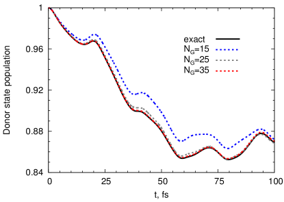
Figure 4: Electronic state population dynamics $\mathrm{tr}\{{\rho}(t)\left|\phi_{1}\right\rangle\left\langle\phi_{1}\right|\}$ for the exact and constrained NOSSEEqs. (65) and (56) formalism with different number $N_{G}$ of basis functions. This figure is reproduced from Ref. ⁷²

Table 1: RMSD for the trace of the density matrix $\mathrm{tr}\{{\rho}\}$ unsing the constrained TDVPEq. (53) compared to the unconstrained approach for different number $N_{G}$ of basis functions.

$N_{G}$	$15$	$25$	$35$
Constrained	$<10^{-5}$	$<10^{-5}$	$<10^{-5}$
Unconstrained	$8.8\cdot 10^{-2}$	$2.8\cdot 10^{-2}$	$6.5\cdot 10^{-3}$

Table 2: RMSD of the molecular system energy in units of $\omega_{1}$ for TDVP combined with NOSSEEqs. (65)-(67) compared to the usual QME approach for different number $N_{G}$ of basis functions.

$N_{G}$	$15$	$25$	$35$
NOSSE	$<10^{-5}$	$<10^{-5}$	$<10^{-5}$
QME	$2.8\cdot 10^{-3}$	$2.3\cdot 10^{-3}$	$2.4\cdot 10^{-3}$

6 Conclusions

Wavefunction ansatzes based on linear combinations of moving FWGs guided by the TDVP provide powerful techniques for modeling nonadiabatic dynamics of both isolated and open molecular systems from first principles. We highlighted several features crucial for performance of this set of techniques. First, among possible electronic state representations, the MCA representation is particularly attractive. It has all the advantages of the diabatic representation and can be directly obtained from electronic structure calculations as the regular adiabatic representation. The only caveat of the MCA use is the non-analytic parametrization of the wavefunction. To avoid problems with the system energy conservation, this feature requires using the stationary action version of the TDVP. Second, if individual nuclear Gaussians are propagated classically (or generally independently) the TDVP application to the FWGs’ amplitudes does not conserve the system energy. This non-conservation is especially pronounced when several Gaussians interfere in the process of dynamics, and it can be related to the basis set incompleteness, which is unavoidable in practice. The only obvious way to conserve the energy is to propagate parameters of individual Gaussians quantum mechanically according to the TDVP in the action formulation. Unfortunately, this makes equations of motion for Gaussian parameters coupled and increase computational complexity of the overall scheme. An interesting question to address is whether there exists a scheme for decoupled Gaussian parameters EOM that conserves the system energy? Third, to address the increase of the wavefunction complexity in time, a systematic extension of the number of nuclear FWGs is needed. Rigorous generalizations of two intuitive schemes for nuclear basis set extension (spawning and cloning) has been discussed. The spawning technique can be rooted in perturbative estimates of population flow between electronic states, while the cloning approach uses estimates of the “decoherence strain” acting on FWGs moving on different PESs. Both schemes can be successfully used for either classically propagated FWGs (e.g. AIMS and MCE) or fully quantum TDVP schemes (e.g. vMCG). Finally, a straightforward generalization of the TDVP to the Liouville equation in order to use FWGs to simulate the reduced density of the open systems encounters two fundamental problems: 1) the total energy of the subsystem in a mixed state is not conserved in the limit of vanishing coupling to the environment, and 2) the subsystem population is not conserved even in the situations when only the energy exchange is allowed. The discussed NOSSE formalism allows to resolve both problems and can be used among other applications for first-principle dynamics of molecules under incoherent light conditions.

7 Acknowledgments

This work was supported by Natural Sciences and Engineering Research Council of Canada (NSERC) through the Discovery Grants Program.

8 Biographical information

Loïc Joubert-Doriol obtained his PhD in 2012 from the University of Montpellier under supervision of Fabien Gatti developing models for nonadiabatic quantum dynamics of molecules interacting with UV/vis light. As a Marie Curie postdoctoral fellow, he worked with Artur Izmaylov and Massimo Olivucci on nonadiabatic quantum effects in biological systems. Since 2016, he develops quantum variational approaches for nonadiabatic dynamics in Izmaylov’s group.

Artur Izmaylov is an Associate Professor at the University of Toronto. He received a PhD with Gustavo Scuseria at Rice University in 2008 and worked as a postdoctoral fellow with John Tully (Yale University) and Michael Frisch (Gaussian Inc.). The main efforts of his group are directed toward developing simulation techniques for quantum molecular dynamics involving multiple electronic states to investigate energy and charge transfer in molecules and nano-structures.

References

- Bakulin et al. 2015 Bakulin, A. A.; Morgan, S. E.; Kehoe, T. B.; Wilson, M. W. B.; Chin, A. W.; Zigmantas, D.; Egorova, D.; Rao, A. Real-time observation of multiexcitonic states in ultrafast singlet fission using coherent 2D electronic spectroscopy. Nat. Chem. 2015, 8, 16–23
- Rao et al. 2016 Rao, B. J.; Gelin, M. F.; Domcke, W. Resonant Femtosecond Stimulated Raman Spectra: Theory and Simulations. J. Phys. Chem. A 2016, 120, 3286–3295
- Zheng et al. 2016 Zheng, J.; Xie, Y.; Jiang, S.; Lan, Z. Ultrafast Nonadiabatic Dynamics of Singlet Fission: Quantum Dynamics with the Multilayer Multiconfigurational Time-Dependent Hartree (ML-MCTDH) Method. J. Phys. Chem. C 2016, 120, 1375–1389
- Wang et al. 2014 Wang, K.; McKoy, V.; Hockett, P.; Schuurman, M. S. Time-Resolved Photoelectron Spectra of : Dynamics at Conical Intersections. Phys. Rev. Lett. 2014, 112, 113007
- Li et al. 2017 Li, Z.; Inhester, L.; Liekhus-Schmaltz, C.; Curchod, B. F.; Snyder, J. W.; Medvedev, N.; Cryan, J.; Osipov, T.; Pabst, S.; Vendrell, O.; Bucksbaum, P.; Martinez, T. J. Ultrafast isomerization in acetylene dication after carbon K-shell ionization. Nat. Commun. 2017, 8, 453
- Vacher et al. 2017 Vacher, M.; Bearpark, M. J.; Robb, M. A.; Malhado, J. P. Electron Dynamics upon Ionization of Polyatomic Molecules: Coupling to Quantum Nuclear Motion and Decoherence. Phys. Rev. Lett. 2017, 118, 083001
- Wu et al. 2015 Wu, G.; Neville, S. P.; Schalk, O.; Sekikawa, T.; Ashfold, M. N. R.; Worth, G. A.; Stolow, A. Excited state non-adiabatic dynamics of pyrrole: A time-resolved photoelectron spectroscopy and quantum dynamics study. J. Chem. Phys. 2015, 142, 074302
- Kirrander et al. 2016 Kirrander, A.; Saita, K.; Shalashilin, D. V. Ultrafast X-ray Scattering from Molecules. J. Chem. Theory Comput. 2016, 12, 957–967
- Makhov et al. 2016 Makhov, D. V.; Martinez, T. J.; Shalashilin, D. V. Toward fully quantum modelling of ultrafast photodissociation imaging experiments. Treating tunnelling in the ab initio multiple cloning approach. Faraday Discuss. 2016, 194, 81–94
- Curchod and Martínez 2018 Curchod, B. F. E.; Martínez, T. J. Ab Initio Nonadiabatic Quantum Molecular Dynamics. Chem. Rev. 2018,
- Makhov et al. 2017 Makhov, D. V.; Symonds, C.; Fernandez-Alberti, S.; Shalashilin, D. V. Ab initio quantum direct dynamics simulations of ultrafast photochemistry with Multiconfigurational Ehrenfest approach. Chem. Phys. 2017, 493, 200–218
- Richings et al. 2015 Richings, G. W.; Polyak, I.; Spinlove, K. E.; Worth, G. A.; Burghardt, I.; Lasorne, B. Quantum dynamics simulations using Gaussian wavepackets: the vMCG method. Int. Rev. Phys. Chem. 2015, 34, 269–308
- Tully 1998 Tully, J. C. Mixed quantum-classical dynamics. Faraday Discuss. 1998, 110, 419
- Tully 2012 Tully, J. C. Perspective: Nonadiabatic dynamics theory. J. Chem. Phys. 2012, 137, 22A301
- Wang et al. 2016 Wang, L.; Akimov, A.; Prezhdo, O. V. Recent Progress in Surface Hopping: 2011–2015. J. Phys. Chem. Lett. 2016, 7, 2100–2112
- Burghardt et al. 2008 Burghardt, I.; Giri, K.; Worth, G. A. Multimode Quantum Dynamics Using Gaussian Wavepackets: The Gaussian-Based Multiconfiguration Time-Dependent Hartree (G-MCTDH) Method Applied to the Absorption Spectrum of Pyrazine. J. Chem. Phys. 2008, 129, 174104
- Burghardt et al. 1999 Burghardt, I.; Meyer, H.-D.; Cederbaum, L. S. Approaches to the approximate treatment of complex molecular systems by the multiconfiguration time-dependent Hartree method. J. Chem. Phys. 1999, 111, 2927–2939
- Meyer et al. 1990 Meyer, H.-D.; Manthe, U.; Cederbaum, L. S. The Multi-Configurational Time-Dependent Hartree Approach. Chem. Phys. Lett. 1990, 165, 73–78
- Wang and Thoss 2003 Wang, H.; Thoss, M. Multilayer Formulation of the Multiconfiguration Time-Dependent Hartree Theory. J. Chem. Phys. 2003, 119, 1289–1299
- Kosloff and Kosloff 1983 Kosloff, D.; Kosloff, R. A Fourier method solution for the time dependent Schrödinger equation as a tool in molecular dynamics. J. Comp. Phys. 1983, 52, 35–53
- Heller 1975 Heller, E. J. Time-dependent approach to semiclassical dynamics. J. Chem. Phys. 1975, 62, 1544–1555
- Heller 1976 Heller, E. J. Time dependent variational approach to semiclassical dynamics. J. Chem. Phys. 1976, 64, 63–73
- Heller 1981 Heller, E. J. Frozen Gaussians: A very simple semiclassical approximation. J. Chem. Phys. 1981, 75, 2923–2931
- Saita and Shalashilin 2012 Saita, K.; Shalashilin, D. V. On-the-fly ab initio molecular dynamics with multiconfigurational Ehrenfest method. J. Chem. Phys. 2012, 137, 22A506
- Worth et al. 2008 Worth, G. A.; Robb, M. A.; Lasorne, B. Solving the Time-Dependent Schrödinger Equation for Nuclear Motion in One Step: Direct Dynamics of Non-Adiabatic Systems. Mol. Phys. 2008, 106, 2077–2091
- Thompson et al. 2010 Thompson, A. L.; Punwong, C.; Martínez, T. J. Optimization of width parameters for quantum dynamics with frozen Gaussian basis sets. Chem. Phys. 2010, 370, 70–77
- Joubert-Doriol et al. 2017 Joubert-Doriol, L.; Sivasubramanium, J.; Ryabinkin, I. G.; Izmaylov, A. F. Topologically Correct Quantum Nonadiabatic Formalism for On-the-Fly Dynamics. J. Phys. Chem. Lett. 2017, 8, 452–456
- Yarkony 1996 Yarkony, D. R. Diabolical conical intersections. Rev. Mod. Phys. 1996, 68, 985–1013
- Migani and Olivucci 2004 Migani, A.; Olivucci, M. In Conical Intersection Electronic Structure, Dynamics and Spectroscopy; Domcke, W., Yarkony, D. R., Köppel, H., Eds.; World Scientific: New Jersey, 2004; p 271
- Meek and Levine 2016 Meek, G. A.; Levine, B. G. Wave Function Continuity and the Diagonal Born-Oppenheimer Correction at Conical Intersections. J. Chem. Phys. 2016, 144, 184109
- Longuet-Higgins et al. 1958 Longuet-Higgins, H. C.; Opik, U.; Pryce, M. H. L.; Sack, R. A. Studies of the Jahn–Teller Effect. II. The Dynamical Problem. Proc. R. Soc. A 1958, 244, 1–16
- Berry 1984 Berry, M. V. Quantal Phase Factors Accompanying Adiabatic Changes. Proc. R. Soc. A 1984, 392, 45–57
- Mead 1992 Mead, C. A. The Geometric Phase in Molecular Systems. Rev. Mod. Phys. 1992, 64, 51–85
- Ryabinkin et al. 2017 Ryabinkin, I. G.; Joubert-Doriol, L.; Izmaylov, A. F. Geometric Phase Effects in Nonadiabatic Dynamics near Conical Intersections. Acc. Chem. Res. 2017, 50, 1785–1793
- Ryabinkin and Izmaylov 2013 Ryabinkin, I. G.; Izmaylov, A. F. Geometric Phase Effects in Dynamics Near Conical Intersections: Symmetry Breaking and Spatial Localization. Phys. Rev. Lett. 2013, 111, 220406
- Joubert-Doriol et al. 2013 Joubert-Doriol, L.; Ryabinkin, I. G.; Izmaylov, A. F. Geometric Phase Effects in Low-Energy Dynamics Near Conical Intersections: A Study of the Multidimensional Linear Vibronic Coupling Model. J. Chem. Phys. 2013, 139, 234103
- Xie et al. 2016 Xie, C.; Ma, J.; Zhu, X.; Yarkony, D. R.; Xie, D.; Guo, H. Nonadiabatic Tunneling in Photodissociation of Phenol. J. Am. Chem. Soc. 2016, 138, 7828–7831
- Joubert-Doriol and Izmaylov 2017 Joubert-Doriol, L.; Izmaylov, A. F. Molecular “topological insulator”: a case study of electron transfer in the bis(methylene) adamantyl carbocation. Chem. Commun. 2017, 53, 7365–7368
- Xie et al. 2018 Xie, C.; Malbon, C. L.; Yarkony, D. R.; Xie, D.; Guo, H. Signatures of a Conical Intersection in Adiabatic Dissociation on the Ground Electronic State. J. Am. Chem. Soc. 2018, 140, 1986–1989
- Li et al. 2017 Li, J.; Joubert-Doriol, L.; Izmaylov, A. F. Geometric phase effects in excited state dynamics through a conical intersection in large molecules: N-dimensional linear vibronic coupling model study. J. Chem. Phys. 2017, 147, 064106
- Henshaw and Izmaylov 2018 Henshaw, S.; Izmaylov, A. F. Topological origins of bound states in the continuum for systems with conical intersections. J. Phys. Chem. Lett. 2018, 9, 146–149
- Mead and Truhlar 1979 Mead, C. A.; Truhlar, D. G. On the Determination of Born–Oppenheimer Nuclear Motion Wave Functions Including Complications Due to Conical Intersections and Identical Nuclei. J. Chem. Phys. 1979, 70, 2284–2296
- Richings and Worth 2017 Richings, G. W.; Worth, G. A. Multi-state non-adiabatic direct-dynamics on propagated diabatic potential energy surfaces. Chem. Phys. Lett. 2017, 683, 606–612
- Meek and Levine 2016 Meek, G. A.; Levine, B. G. The best of both Reps – Diabatized Gaussians on adiabatic surfaces. J. Chem. Phys. 2016, 145, 184103
- Köppel and Schubert 2006 Köppel, H.; Schubert, B. The concept of regularized diabatic states for a general conical intersection. Mol. Phys. 2006, 104, 1069–1079
- Longuet-Higgins 1961 Longuet-Higgins, H. Some recent developments in the theory of molecular energy levels. 1961
- Ballhausen and Hansen 1972 Ballhausen, C.; Hansen, A. E. Electronic spectra. Ann. Rev. Phys. Chem. 1972, 23, 15–38
- Dirac 1930 Dirac, P. A. M. Proc. Cambridge Philos. Soc. 1930, 26, 376–385
- Frenkel 1934 Frenkel, J. Wave Mechanics; Clarendon Press: Oxford, 1934
- McLachlan 1964 McLachlan, A. D. A variational solution of the time-dependent Schrodinger equation. Mol. Phys. 1964, 8, 39–44
- Broeckhove et al. 1988 Broeckhove, J.; Lathouwers, L.; Kesteloot, E.; Van Leuven, P. On the equivalence of time-dependent variational principles. Chem. Phys. Lett. 1988, 149, 547–550
- Kan 1981 Kan, K.-K. Equivalence of time-dependent variational descriptions of quantum systems and Hamilton’s mechanics. Phys. Rev. A 1981, 24, 2831–2834
- Ben-Nun and Martinez 2002 Ben-Nun, M.; Martinez, T. J. Ab Initio Quantum Molecular Dynamics. Adv. Chem. Phys. 2002, 121, 439–512
- Yang et al. 2009 Yang, S.; Coe, J. D.; Kaduk, B.; Martínez, T. J. An “Optimal” Spawning Algorithm for Adaptive Basis Set Expansion in Nonadiabatic Dynamics. J. Chem. Phys. 2009, 130, 134113
- Habershon 2012 Habershon, S. Linear dependence and energy conservation in Gaussian wavepacket basis sets. J. Chem. Phys. 2012, 136, 014109
- Helgaker et al. 2000 Helgaker, T.; Jorgensen, P.; Olsen, J. Molecular Electronic-Structure Theory; Wiley: Chichester, 2000
- Joubert-Doriol and Izmaylov 2018 Joubert-Doriol, L.; Izmaylov, A. F. Variational nonadiabatic dynamics in the moving crude adiabatic representation: Further merging of nuclear dynamics and electronic structure. J. Chem. Phys. 2018, 148, 114102
- Makhov et al. 2014 Makhov, D. V.; Glover, W. J.; Martinez, T. J.; Shalashilin, D. V. Ab Initio Multiple Cloning Algorithm for Quantum Nonadiabatic Molecular Dynamics. J. Chem. Phys. 2014, 141, 054110
- Izmaylov et al. 2011 Izmaylov, A. F.; Mendive Tapia, D.; Bearpark, M. J.; Robb, M. A.; Tully, J. C.; Frisch, M. J. Nonequilibrium Fermi golden rule for electronic transitions through conical intersections. J. Chem. Phys. 2011, 135, 234106
- Endicott et al. 2014 Endicott, J. S.; Joubert-Doriol, L.; Izmaylov, A. F. A perturbative formalism for electronic transitions through conical intersections in a fully quadratic vibronic model. J. Chem. Phys. 2014, 141, 034104
- Izmaylov 2013 Izmaylov, A. F. Perturbative Wave-Packet Spawning Procedure for Non-Adiabatic Dynamics in Diabatic Representation. J. Chem. Phys. 2013, 138, 104115
- Gershgorn and Shavitt 1968 Gershgorn, Z.; Shavitt, I. An application of perturbation theory ideas in configuration interaction calculations. Int. J. Quant. Chem. 1968, 2, 751–759
- Davidson et al. 1981 Davidson, E. R.; McMurchie, L. E.; Day, S. J. The BK method: Application to methylene. J. Chem. Phys. 1981, 74, 5491–5496
- Hahn and Stock 2000 Hahn, S.; Stock, G. Quantum-Mechanical Modeling of the Femtosecond Isomerization in Rhodopsin. J. Phys. Chem. B 2000, 104, 1146–1149
- Moix et al. 2011 Moix, J.; Wu, J.; Huo, P.; Coker, D.; Cao, J. Efficient Energy Transfer in Light-Harvesting Systems, III: The Influence of the Eighth Bacteriochlorophyll on the Dynamics and Efficiency in FMO. J. Phys. Chem. Lett. 2011, 2, 3045–3052
- Tscherbul and Brumer 2014 Tscherbul, T. V.; Brumer, P. Excitation of Biomolecules with Incoherent Light: Quantum Yield for the Photoisomerization of Model Retinal. J. Phys. Chem. A 2014, 118, 3100–3111
- Tscherbul and Brumer 2015 Tscherbul, T. V.; Brumer, P. Quantum coherence effects in natural light-induced processes: cis – trans photoisomerization of model retinal under incoherent excitation. Phys. Chem. Chem. Phys. 2015, 17, 30904–30913
- Nitzan 2006 Nitzan, A. Chemical dynamics in condensed phase; Oxford University Press: New York, 2006
- Breuer and Petruccione 2002 Breuer, H.-P.; Petruccione, F. The theory of open quantum systems; Oxford University Press: Oxford, 2002
- Raab and Meyer 2000 Raab, A.; Meyer, H.-D. Multiconfigurational expansions of density operators: equations of motion and their properties. Theor. Chem. Acc. 2000, 104, 358–369
- Gerdts and Manthe 1997 Gerdts, T.; Manthe, U. A wave packet approach to the Liouville–von Neumann equation for dissipative systems. J. Chem. Phys. 1997, 106, 3017–3023
- Joubert-Doriol and Izmaylov 2015 Joubert-Doriol, L.; Izmaylov, A. F. Problem-free time-dependent variational principle for open quantum systems. J. Chem. Phys. 2015, 142, 134107
- Dalton et al. 2014 Dalton, B. J.; Jeffers, J.; Barnett, S. M. Phase space methods for degenerate quantum gases; Oxford University Press: Oxford, 2014; Vol. 163
- Joubert-Doriol et al. 2014 Joubert-Doriol, L.; Ryabinkin, I. G.; Izmaylov, A. F. Non-stochastic matrix Schrödinger equation for open systems. J. Chem. Phys. 2014, 141, 234112
- Kressner et al. 2009 Kressner, D.; Schröder, C.; Watkins, D. S. Implicit QR algorithms for palindromic and even eigenvalue problems. Numer. Algor. 2009, 51, 209–238
- Lindblad 1976 Lindblad, G. On the generators of quantum dynamical semigroups. Commun. Math. Phys. 1976, 48, 119–130
- Takagahara et al. 1978 Takagahara, T.; Hanamura, E.; Kubo, R. Second Order Optical Processes in a Localized Electron-Phonon System -Stationary Response. J. Phys. Soc. Japan 1978, 44, 728–741
- Wolfseder and Domcke 1995 Wolfseder, B.; Domcke, W. Multi-mode vibronic coupling with dissipation. Application of the Monte Carlo wavefunction propagation method. Chem. Phys. Lett. 1995, 235, 370–376