On the Regularizing Property of Stochastic Gradient Descent

Abstract

Stochastic gradient descent (SGD) and its variants are among the most successful approaches for solving large-scale optimization problems. At each iteration, SGD employs an unbiased estimator of the full gradient computed from one single randomly selected data point. Hence, it scales well with problem size and is very attractive for handling truly massive dataset, and holds significant potentials for solving large-scale inverse problems. In this work, we rigorously establish its regularizing property under a priori early stopping rule for linear inverse problems, and also prove convergence rates under the canonical sourcewise condition. This is achieved by combining tools from classical regularization theory and stochastic analysis. Further, we analyze its preasymptotic weak and strong convergence behavior, in order to explain the fast initial convergence typically observed in practice. The theoretical findings shed insights into the performance of the algorithm, and are complemented with illustrative numerical experiments.
Keywords: stochastic gradient descent; regularizing property; error estimates; preasymptotic convergence.

1 Introduction

In this paper, we consider the following finite-dimensional linear inverse problem:

$$Ax=y^{\dagger},$$ (1.1)

where $A\in\mathbb{R}^{n\times m}$ is a matrix representing the data formation mechanism, $x\in\mathbb{R}^{m}$ is the unknown signal of interest, and $y^{\dagger}\in\mathbb{R}^{n}$ is the exact data formed by $y^{\dagger}=Ax^{\dagger}$, with $x^{\dagger}$ being the true solution. In practice, we can only access the noisy data $y^{\delta}\in\mathbb{R}^{n}$ defined by

$$y^{\delta}=y^{\dagger}+\xi,$$

where the vector $\xi\in\mathbb{R}^{n}$ is the noise in the data, with a noise level $\delta=\|\xi\|$ (and $\bar{\delta}=n^{-\frac{1}{2}}\delta$). The noise $\xi$ is assumed to be a realization of an independent identically distributed (i.i.d.) mean zero Gaussian random vector. Throughout, we denote the $i$th row of the matrix $A$ by a column vector $a_{i}\in\mathbb{R}^{m}$, and the $i$th entry of the vector $y^{\delta}$ by $y_{i}^{\delta}$. The model (1.1) is representative of many discrete linear inverse problems, including linearized (sub)problems of nonlinear inverse problems. Hence, the stable and efficient numerical solution of the model (1.1) has been the topic of many research works, and plays an important role in developing practical inversion techniques (see, e.g., [8, 9]).

Stochastic gradient descent (SGD), dated at least back to Robbins and Monro [23], represents an extremely popular solver for large-scale least square type problems and statistical inference, and its accelerated variants represent state-of-the-art solvers for training (deep) neural networks [4, 14, 5]. Such methods hold significant potentials for solving large-scale inverse problems. For example, the randomized Kaczmarz method [25], which has long been very popular and successful in computed tomography [18], can be viewed as SGD with weighted sampling (see, e.g., [19] and [12, Prop. 4.1]). Besides the randomized Kaczmarz method, there are also several experimental evaluations on SGD for inverse problems [11, 6]. Hence, it is extremely important to understand theoretical properties of such stochastic reconstruction methods, which, to the best of our knowledge, have not been addressed in the context of ill-posed inverse problems.

In this work, we contribute to the theoretical analysis of SGD for inverse problems. Consider the following basic version of SGD: given an initial guess $x_{1}\in\mathbb{R}^{m}$, update the iterate $x_{k+1}^{\delta}$ by

$$x_{k+1}^{\delta}=x_{k}^{\delta}-\eta_{k}((a_{i_{k}},x_{k}^{\delta})-y_{i_{k}}^{\delta})a_{i_{k}},\quad k=1,\ldots$$ (1.2)

where the index $i_{k}$ is drawn i.i.d. uniformly from the set $\{1,\ldots,n\}$, $\eta_{k}>0$ is the step size at the $k$th iteration, and $(\cdot,\cdot)$ denotes the Euclidean inner product on $\mathbb{R}^{m}$. The update (1.2) can be derived by computing an unbiased gradient estimate $((a_{i_{k}},x)-y_{i_{k}}^{\delta})a_{i_{k}}$ from the functional $\frac{1}{2}(y_{i_{k}}^{\delta}-(a_{i_{k}},x))^{2}$ for a randomly sampled single datum $\{a_{i_{k}},y_{i_{k}}^{\delta}\}$, instead of the gradient $n^{-1}A^{t}(Ax-y^{\delta})$ of the functional $\frac{1}{2n}\sum_{i=1}^{n}(y_{i}^{\delta}-(a_{i},x))^{2}$ for the full data. Thus, the SGD iteration (1.2) is a randomized version of the classical Landweber iteration:

$$x_{k+1}^{\delta}=x_{k}^{\delta}-\eta_{k}n^{-1}A^{t}(Ax_{k}^{\delta}-y^{\delta}).$$ (1.3)

In comparison with Landweber iteration (1.3), SGD requires only evaluating one datum $\{a_{i_{k}},y_{i_{k}}^{\delta}\}$ per iteration, and thus the per-iteration cost is drastically reduced, which is especially attractive for large-scale problems. In theory, Landweber method is known to be regularizing [8, Chapter 6]. However, the regularizing property of SGD remains to be established, even though it was conjectured and empirically examined (see, e.g., [24, 10, 28]). Numerically, one observes a semiconvergence phenomenon for SGD: the iterate $x_{k}^{\delta}$ first converges to the true solution $x^{\dagger}$, and then diverges as the iteration further proceeds. Semiconvergence is characteristic of (deterministic) iterative regularization methods, and early stopping is often employed [8, 15]. Below we describe the main theoretical contributions of this work, which are complemented with numerical experiments in Section 6.

The first contribution is to analyze SGD with a polynomially decaying sequence of step sizes (see Assumption 2.1) through the lens of regularization theory. In Theorems 2.1 and 2.2, we prove that SGD is regularizing in the sense that iterate $x_{k}^{\delta}$ converges to the exact solution $x^{\dagger}$ in the mean squared norm as the noise level $\delta$ tends to zero, under a priori early stopping rule, and also $x_{k}^{\delta}$ converges to $x^{\dagger}$ at certain rates under canonical source condition. To the best of our knowledge, this is the first result on regularizing property of a stochastic iteration method. The analysis relies on decomposing the error into three components: approximation error due to early stopping, propagation error due to the presence of data noise, and stochastic error due to the random index $i_{k}$. The first two parts are deterministic and can be analyzed in a manner similar to Landweber method [8, Chapter 6]; see Theorem 3.1 and 3.2. The last part on the variance of the iterate constitutes the main technical challenge in the analysis. It is overcome by relating the iterate variance to the expected square residuals and analyzing the evolution of the latter; see Theorems 3.3 and 3.4.

The second contribution is to analyze the preasymptotic convergence in both weak and strong sense. In practice, it is often observed that SGD can decrease the error very fast during initial iterations. We provide one explanation of the phenomenon by means of preasymptotic convergence, which extends the recent work on the randomized Kaczmarz method [12]. It is achieved by dividing the error into low- and high-frequency components according to right singular vectors, and studying their dynamics separately. In Theorems 2.3 and 2.4, we prove that the low-frequency error can decay much faster than the high-frequency one in either weak or strong norm. In particular, if the initial error is dominated by the low-frequency components, then SGD decreases the total error very effectively during the first iterations. The analysis sheds important insights into practical performance of SGD. Further, under the canonical source type condition, the low-frequency error is indeed dominating, cf. Proposition 5.1.

Now we situate this work in the existing literature in two related areas: inverse problems with random noise, and machine learning. Inverse problems with random noise have attracted much attention over the last decade. In a series of works, Hohage and his collaborators [1, 2, 3] studied various regularization methods, e.g., Tikhonov and iterative regularization, for solving linear and nonlinear inverse problems with random noise. For example, Bissantz et al [2] analyzed Tikhonov regularization for nonlinear inverse problems, and analyzed consistency and convergence rate. In these works, randomness enters into the problem formulation via the data $y^{\delta}$ directly as a Hilbert space valued process, which is fixed (though random) when applying regularization techniques. Thus, it differs greatly from SGD, for which randomness arises due to the random row index $i_{k}$ and changes at each iteration. Handling the iteration noise requires different techniques than that in these works.

There are also several relevant works in the context of machine learning [27, 26, 17, 7]. Ying and Pontil [27] studied an online least-squares gradient descent algorithm in a reproducing kernel Hilbert space (RKHS), and presented a novel capacity independent approach to derive bounds on the generalization error. Tarres and Yao [26] analyzed the convergence of a (regularized) online learning algorithm closely related to SGD. Lin and Rosasco [17] analyzed the influence of batch size on the convergence of mini-batch SGD. See also the recent work [7] on SGD with averaging for nonparametric regression in RKHS. All these works analyze the method in the framework of statistical learning, where the noise arises mainly due to finite sampling of the (unknown) underlying data distribution, whereas for inverse problems, the noise arises from imperfect data acquisition process and enters into the data $y^{\delta}$ directly. Further, the main focus of these works is to bound the generalization error, instead of error estimates for the iterate. Nonetheless, our proof strategy in decomposing the total error into three different components shares similarity with these works.

The rest of the paper is organized as follows. In Section 2, we present and discuss the main results, i.e., regularizing property and preasymptotic convergence. In Section 3, we derive bounds on three parts of the total error. Then in Section 4, we analyze the regularizing property of SGD with a priori stopping rule, and prove convergence rates under classical source condition. In Section 5, we discuss the preasymptotic convergence of SGD. Some numerical results are given in Section 6. In an appendix, we collect some useful inequalities. We conclude this section with some notation. We use the superscript $\delta$ in $x_{k}^{\delta}$ to indicate SGD iterates for noisy data $y^{\delta}$, and denote by $x_{k}$ that for the exact data $y^{\dagger}$. The notation $\|\cdot\|$ denotes Euclidean norm for vectors and spectral norm for matrices, and $[\cdot]$ denotes the integral part of a real number. $\{\mathcal{F}_{k}\}_{k\geq 1}$ denotes a sequence of increasing $\sigma$-fields generated by the random index $i_{k}$ up to the $k$th iteration. The notation $c$, with or without subscript, denotes a generic constant that is always independent of the iteration index $k$ and the noise level $\delta$.

2 Main results and discussions

In this part, we present the main results of the work, i.e., regularizing property of SGD and preasymptotic convergence results. The detailed proofs are deferred to Sections 4 and 5, which in turn rely on technical estimates derived in Section 3. Throughout, we consider the following step size schedule, which is commonly employed for SGD.

Assumption 2.1.

The step size $\eta_{j}=c_{0}j^{-\alpha}$, $j=1,2,\ldots,$ $\alpha\in(0,1)$, with $c_{0}\max_{i}\|a_{i}\|^{2}\leq 1$.

Due to stochasticity of the row index $i_{k}$, the iterate $x_{k}^{\delta}$ is random. We measure the approximation error $x_{k}^{\delta}-x^{\dagger}$ to the true solution $x^{\dagger}$ by the mean squared error $\mathbb{E}[\|x_{k}^{\delta}-x^{\dagger}\|^{2}]$, where the expectation $\mathbb{E}[\cdot]$ is with respect to the random index $i_{k}$. The reference solution $x^{\dagger}$ is taken to be the unique minimum norm solution (relative to the initial guess $x_{1}$):

$$x^{\dagger}=\arg\min_{x\in\mathbb{R}^{m}}\left\{\|x-x_{1}\|\quad\mbox{s.t.}\quad Ax^{\dagger}=y^{\dagger}\right\}.$$ (2.1)

Now we can state the regularizing property of SGD (1.2) under a priori stopping rule: the error $\mathbb{E}[\|x_{k(\delta)}^{\delta}-x^{\dagger}\|^{2}]$ tends to zero as the noise level $\delta\to 0$, if the stopping index $k(\delta)$ is chosen properly in relation to the noise level $\delta$. Thus, SGD equipped with suitable a priori stopping rule is a regularization method. Note that condition (2.2) is analogous to that for classical regularization methods.

Theorem 2.1.

Let Assumption 2.1 be fulfilled. If the stopping index $k(\delta)$ satisfies

$$\lim_{\delta\to 0^{+}}k(\delta)=\infty\quad\mbox{and}\quad\lim_{\delta\to 0^{+}}k(\delta)^{\frac{\alpha-1}{2}}\delta=0,$$ (2.2)

then the iterate $x_{k(\delta)}^{\delta}$ satisfies

$$\lim_{\delta\to 0^{+}}\mathbb{E}[\|x_{k(\delta)}^{\delta}-x^{\dagger}\|^{2}]=0.$$

To derive convergence rates, we employ the source condition in classical regularization theory [8, 9]. Recall that the canonical source condition reads: there exists some $w\in\mathbb{R}^{m}$ such that

$$x^{\dagger}-x_{1}=B^{p}w,\quad p\geq 0,$$ (2.3)

where the symmetric and positive semidefinite $B\in\mathbb{R}^{m\times m}$ is defined in (3.4) below, and $B^{p}$ denotes the usual fractional power (via spectral decomposition). Condition (2.3) represents a type of smoothness of the initial error $x^{\dagger}-x_{1}$, and the exponent $p$ determines the degree of smoothness: the larger the exponent $p$ is, the smoother the initial error $x^{\dagger}-x_{1}$ becomes. It controls the approximation error due to early stopping (see Theorem 3.1 below for the precise statement). The source type condition is one of the most classical approaches to derive convergence rates in classical regularization theory [8, 9].

Next we can state convergence rates under a priori stopping index.

Theorem 2.2.

Let Assumption 2.1 and the source condition (2.3) be fulfilled. Then there holds

$$\mathbb{E}[\|x_{k+1}^{\delta}-x^{\dagger}\|^{2}]\leq ck^{-\min(2\alpha,\min(1,2p)(1-\alpha))}\ln^{2}k+c^{\prime}k^{1-\alpha}\bar{\delta}^{2}+c^{\prime\prime}\delta^{2},$$

where the constants $c,c^{\prime}$ and $c^{\prime\prime}$ depend on $\alpha,p,\|w\|,\|Ax_{1}-y^{\delta}\|$ and $\|A\|$.

Remark 2.1.

Theorem 2.2 indicates a semiconvergence for the iterate $x_{k}^{\delta}$: the first term is decreasing in $k$ and dependent of regularity index $p$ and the step size parameter $\alpha\in(0,1)$, and the second term $k^{1-\alpha}\bar{\delta}^{2}$ is increasing in $k$ and dependent of the noise level. The first term $k^{-\min(2\alpha,\min(1,2p)(1-\alpha))}\ln^{2}k$ contains both approximation error (indicated by $p$) and stochastic error. By properly balancing the first two terms in the estimate, one can obtain a convergence rate. The best possible convergence rate depends on both the decay rate $\alpha$ and the regularity index $p$ in (2.3), and it is suboptimal for any $p>\frac{1}{2}$ when compared with Landweber method. That is, the vanilla SGD seems to suffer from saturation, due to the stochasticity induced by the random row index $i_{k}$.

In practice, it is often observed that SGD decreases the error rapidly during the initial iterations. This phenomenon cannot be explained by the regularizing property. Instead, we analyze the preasymptotic convergence by means of SVD, in order to explain the fast initial convergence. Let $n^{-\frac{1}{2}}A=U\Sigma V^{t}$, where $U\in\mathbb{R}^{n\times n},V=[v_{1}\ v_{2}\ \cdots\ v_{m}]\in\mathbb{R}^{m\times m}$ are orthonormal, and $\Sigma=\mathrm{diag}(\sigma_{1},\ldots,\sigma_{r},0,\ldots,0)\in\mathbb{R}^{n\times m}$ is diagonal with the diagonals ordered nonincreasingly and $r$ the rank of $A$. For any fixed truncation level $1\leq L\leq r$, we define the low- and high-frequency solution spaces $\mathcal{L}$ and $\mathcal{H}$ respectively by

$$\mathcal{L}=\mathrm{span}(\{v_{i}\}_{i=1}^{L})\quad\mbox{and}\quad\mathcal{H}=\mathrm{span}(\{v\}_{i=L+1}^{\min(n,m)}).$$

Let $P_{\mathcal{L}}$ and $P_{\mathcal{H}}$ be the orthogonal projection onto $\mathcal{L}$ and $\mathcal{H}$, respectively. The analysis relies on decomposing the error $e_{k}^{\delta}=x_{k}^{\delta}-x^{\dagger}$ into the low- and high-frequency components $P_{\mathcal{L}}e_{k}^{\delta}$ and $P_{\mathcal{H}}e_{k}^{\delta}$, respectively, in order to capture their essentially different dynamics.

We have the following preasymptotic weak and strong convergence results, which characterize the one-step evolution of the low- and high-frequency errors. The proofs are given in Section 5.

Theorem 2.3.

If $\eta_{k}\leq c_{0}$ with $c_{0}\max_{i}\|a_{i}\|^{2}\leq 1$, then there hold

$$\|\mathbb{E}[P_{\mathcal{L}}e_{k+1}^{\delta}]\| \leq(1-\eta_{k}\sigma_{L}^{2})\|\mathbb{E}[P_{\mathcal{L}}e_{k}^{\delta}]\|+c_{0}^{-\frac{1}{2}}\eta_{k}\bar{\delta},$$

$$\|\mathbb{E}[P_{\mathcal{H}}e_{k+1}^{\delta}]\| \leq\|\mathbb{E}[P_{\mathcal{H}}e_{k}^{\delta}]\|+\eta_{k}\sigma_{L+1}\bar{\delta}.$$

Theorem 2.4.

If $\eta_{k}\leq c_{0}$ with $c_{0}\max_{i}\|a_{i}\|^{2}\leq 1$, then with $c_{1}=\sigma_{L}^{2}$, and $c_{2}=\sum_{i=L+1}^{r}\sigma_{i}^{2}$, there hold

$$\mathbb{E}[\|P_{\mathcal{L}}e_{k+1}^{\delta}\|^{2}|\mathcal{F}_{k-1}] \leq(1-c_{1}\eta_{k})\|P_{\mathcal{L}}e_{k}^{\delta}\|^{2}+c_{2}c_{0}^{-1}\eta_{k}^{2}\|P_{\mathcal{H}}e_{k}^{\delta}\|^{2}+c_{0}^{-1}\eta_{k}\bar{\delta}(\eta_{k}\bar{\delta}+2\sqrt{2}\sigma_{1}\|e_{k}^{\delta}\|),$$

$$\mathbb{E}[\|P_{\mathcal{H}}e_{k+1}^{\delta}\|^{2}|\mathcal{F}_{k-1}] \leq c_{2}c_{0}^{-1}\eta_{k}^{2}\|P_{\mathcal{L}}e_{k}^{\delta}\|^{2}+(1+c_{2}c_{0}^{-1}\eta_{k}^{2})\|P_{\mathcal{H}}e_{k}^{\delta}\|^{2}+c_{0}^{-1}\eta_{k}^{2}\bar{\delta}^{2}$$

$$\quad+2\sqrt{2}c_{2}^{\frac{1}{2}}\eta_{k}\bar{\delta}\Big{(}\|P_{\mathcal{H}}e_{k}^{\delta}\|^{2}+c_{0}^{-2}\eta_{k}^{2}\|e_{k}^{\delta}\|^{2}\Big{)}^{\frac{1}{2}}.$$

Remark 2.2.

It is noteworthy that in Theorems 2.3 and 2.4, the step size $\eta_{k}$ is not required to be polynomially decaying. Theorems 2.3 and 2.4 indicate that the low-frequency error can decrease much faster than the high-frequency error in either the weak or mean squared norm sense. Thus, if the initial error $e_{1}$ consists mostly of low-frequency modes, SGD can decrease the low-frequency error and thus also the total error rapidly, resulting in fast initial convergence.

3 Preliminary estimates

In this part, we provide several technical estimates for the SGD iteration (1.2). By bias-variance decomposition and triangle inequality, we have

$$\mathbb{E}[\|x_{k}^{\delta}-x^{\dagger}\|^{2}] =\|\mathbb{E}[x_{k}^{\delta}]-x^{\dagger}\|^{2}+\mathbb{E}[\|\mathbb{E}[x_{k}^{\delta}]-x_{k}^{\delta}\|^{2}]$$

$$\leq 2\|\mathbb{E}[x_{k}]-x^{\dagger}\|^{2}+2\|\mathbb{E}[x_{k}-x_{k}^{\delta}]\|^{2}+\mathbb{E}[\|\mathbb{E}[x_{k}^{\delta}]-x_{k}^{\delta}\|^{2}],$$ (3.1)

where $x_{k}$ is the random iterate for exact data $y^{\dagger}$. Thus, the total error is decomposed into three components: approximation error due to early stopping, propagation error due to noise and stochastic error due to the random index $i_{k}$. The objective below is to derive bounds on the three terms in (3.1), which are crucial for proving Theorems 2.1 and 2.2 in Section 4. The approximation and propagation errors are given in Theorems 3.1 and 3.2, respectively. The stochastic error is analyzed in Section 3.2: first in terms of the expected squared residuals in Theorem 3.3, and then bound on the latter in Theorem 3.4. The analysis of the stochastic error represents the main technical challenge.

3.1 Approximation and propagation errors

For the analysis, we first introduce auxiliary iterations. Let $e_{k}^{\delta}=x_{k}^{\delta}-x^{\dagger}$ and $e_{k}=x_{k}-x^{\dagger}$ be the errors for SGD iterates $x_{k}^{\delta}$ and $x_{k}$, for $y^{\delta}$ and $y^{\dagger}$, respectively. They satisfy the following recursion:

$$e_{k+1} =e_{k}-\eta_{k}((a_{i_{k}},x_{k})-y_{i_{k}}^{\dagger})a_{i_{k}}=e_{k}-\eta_{k}(a_{i_{k}},e_{k})a_{i_{k}},$$ (3.2)

$$e_{k+1}^{\delta} =e_{k}^{\delta}-\eta_{k}((a_{i_{k}},x_{k}^{\delta})-y_{i_{k}}^{\delta})a_{i_{k}}=e_{k}^{\delta}-\eta_{k}(a_{i_{k}},e_{k}^{\delta})a_{i_{k}}+\eta_{k}\xi_{i_{k}}a_{i_{k}}.$$ (3.3)

Then we introduce two auxiliary matrices: for any vector $b\in\mathbb{R}^{n}$,

$$B:=\mathbb{E}[a_{i}a_{i}^{t}]\quad\mbox{and}\quad\bar{A}^{t}b:=\mathbb{E}[a_{i}b_{i}].$$ (3.4)

Under i.i.d. uniform sampling of the index $i_{k}$, $B=n^{-1}A^{t}A$ and $\bar{A}^{t}=n^{-1}A^{t}$. Below, let

$$\Pi_{j}^{k}(B)=\prod_{i=j}^{k}(I-\eta_{i}B),\quad j\leq k,$$ (3.5)

with the convention $\Pi_{k+1}^{k}(B)=I$,

Now we bound the weighted norm $\|B^{s}\mathbb{E}[e_{k}]\|$ of the approximation error $\mathbb{E}[e_{k}]$. The cases $s=0$ and $s=1/2$ will be used for bounding the approximation error and the residual, respectively.

Theorem 3.1.

Let Assumption 2.1 be fulfilled. Under the source condition (2.3) and for any $s\geq 0$, with $c_{p,s}=(\frac{(p+s)(1-\alpha)}{c_{0}e(2^{1-\alpha}-1)})^{p+s}\|w\|$, there holds

$$\|B^{s}\mathbb{E}[e_{k+1}]\|\leq c_{p,s}k^{-(p+s)(1-\alpha)}.$$

Proof.

It follows from (3.2) and the identity $y_{i}^{\dagger}=(a_{i},x^{\dagger})$ that the error $e_{k}$ satisfies

$$\mathbb{E}[e_{k+1}|\mathcal{F}_{k-1}] =(I-\eta_{k}\mathbb{E}[a_{i}a_{i}^{t}])e_{k}=(I-\eta_{k}B)e_{k}.$$

Taking the full expectation yields

$$\mathbb{E}[e_{k+1}]=(I-\eta_{k}B)\mathbb{E}[e_{k}].$$ (3.6)

Repeatedly applying the recursion (3.6) and noting that $e_{1}$ is deterministic give

$$\mathbb{E}[e_{k+1}]=\prod_{i=1}^{k}(I-\eta_{i}B)\mathbb{E}[e_{1}]=\prod_{i=1}^{k}(I-\eta_{i}B)e_{1}.$$

From the source condition (2.3), we deduce

$$\|B^{s}\mathbb{E}[e_{k+1}]\|\leq\|\Pi_{1}^{k}(B)B^{p+s}\|\|w\|.$$

By Lemmas A.1 and A.2, we arrive at

$$\|\mathbb{E}[e_{k+1}]\| \leq\frac{(p+s)^{p+s}}{e^{p+s}(\sum_{i=1}^{k}\eta_{i})^{p+s}}\|w\|\leq c_{p,s}k^{-(p+s)(1-\alpha)},$$

with a constant $c_{p,s}=(\frac{(p+s)(1-\alpha)}{c_{0}e(2^{1-\alpha}-1)})^{p+s}\|w\|$. This completes the proof of the theorem. ∎

Remark 3.1.

The constant $c_{p,s}$ is uniformly bounded in $\alpha\in[0,1]$: $\lim_{\alpha\to 1^{-}}\frac{1-\alpha}{2^{1-\alpha}-1}=\frac{1}{\ln 2}$.

Next we bound the weighted norm of the propagation error $\mathbb{E}[x_{k}^{\delta}-x_{k}]$ due to data noise $\xi$.

Theorem 3.2.

Let Assumption 2.1 be fulfilled, $s\in[-\frac{1}{2},\frac{1}{2}]$, and $r=\frac{1}{2}+s$. Then there holds

$$\|B^{s}\mathbb{E}[x_{k+1}-x_{k+1}^{\delta}]\|\leq c_{r,\alpha}\bar{\delta}\left\{\begin{array}[]{ll}k^{(1-r)(1-\alpha)},&0\leq r<1,\\ \max(1,\ln k),&r=1,\end{array}\right.$$

with $c_{r,\alpha}$ given by

$$c_{r,\alpha}=c_{0}^{1-r}\left\{\begin{array}[]{ll}\frac{r^{r}}{e^{r}}B(1-\alpha,1-r)+1,&r<1,\\ \frac{r^{r}}{e^{r}}2^{\alpha}\frac{2-\alpha}{1-\alpha}+1,&r=1.\end{array}\right.$$

Proof.

By the recursions (3.2) and (3.3), the propagation error $\nu_{k}=\mathbb{E}[x_{k}^{\delta}-x_{k}]$ satisfies $\nu_{1}=0$ and $\nu_{k+1}=(I-\eta_{k}B)\nu_{k}+\eta_{k}\bar{A}^{t}\xi$, with $\xi=y^{\delta}-y^{\dagger}$. Applying the recursion repeatedly yields

$$\nu_{k+1}=\sum_{j=1}^{k}\eta_{j}\Pi_{j+1}^{k}(B)\bar{A}^{t}\xi.$$

Thus, by the triangle inequality, we have

$$\|B^{s}\nu_{k+1}\|\leq\sum_{j=1}^{k}\eta_{j}\|B^{s}\Pi_{j+1}^{k}(B)\bar{A}^{t}\|\|\xi\|.$$

Since $\|B^{s}\Pi_{j+1}^{k}(B)\bar{A}^{t}\|=n^{-\frac{1}{2}}\|\Pi_{j+1}^{k}(B)B^{s+\frac{1}{2}}\|$, by Lemma A.1,

$$\|B^{s}\nu_{k+1}\| \leq\frac{r^{r}}{e^{r}}\sum_{j=1}^{k-1}\frac{\eta_{j}}{(\sum_{i=j+1}^{k}\eta_{i})^{r}}\bar{\delta}+\eta_{k}\|B^{s}\bar{A}^{t}\|\|\xi\|$$

$$=\Big{(}\frac{r^{r}}{e^{r}}\sum_{j=1}^{k-1}\frac{\eta_{j}}{(\sum_{i=j+1}^{k}\eta_{i})^{r}}+k^{-\alpha}c_{0}\|B\|^{r}\Big{)}\bar{\delta}.$$

Under Assumption 2.1, we have $c_{0}\|B\|^{r}\leq c_{0}^{1-r}$. This and Lemma A.2 complete the proof. ∎

Remark 3.2.

The iterate means $\mathbb{E}[x_{k}]$ and $\mathbb{E}[x_{k}^{\delta}]$ satisfy the recursion for Landweber method (LM). Hence, the proof and error bounds resemble closely that for LM [8, Chapter 6]. Taking $s=0$ in Theorems 3.1 and 3.2 yields

$$\|\mathbb{E}[x_{k+1}^{\delta}]-x^{\dagger}\|\leq c_{p}k^{-p(1-\alpha)}+c_{\alpha}k^{\frac{1-\alpha}{2}}\bar{\delta}.$$

By balancing the two terms, one can derive a convergence rate in terms of $\bar{\delta}$ (instead of $\delta$), and this is achieved quickest by $\alpha=0$. Such an estimate is known as weak error in the literature of stochastic differential equations. By bias variance decomposition, it is weaker than the mean squared error.

3.2 Stochastic error

The next result gives a bound on the variance $\mathbb{E}[\|B^{s}(x_{k}^{\delta}-\mathbb{E}[x_{k}^{\delta}])\|^{2}]$. It arises from the random index $i_{k}$ in SGD (1.2). Theorem 3.3 relates the variance to the past mean squared residuals $\{\mathbb{E}[\|Ax_{j}^{\delta}-y^{\delta}\|^{2}]\}_{j=1}^{k}$ and step sizes $\{\eta_{j}\}_{j=1}^{k}$. The extra exponent $\frac{1}{2}$ follows from the quadratic structure of the least-squares functional.

Theorem 3.3.

For the SGD iteration (1.2), there holds

$$\mathbb{E}[\|B^{s}(x_{k+1}^{\delta}-\mathbb{E}[x_{k+1}^{\delta}])\|^{2}]\leq\sum_{j=1}^{k}\eta_{j}^{2}\|B^{s+\frac{1}{2}}\Pi_{j+1}^{k}(B)\|^{2}\mathbb{E}[\|Ax_{j}^{\delta}-y^{\delta}\|^{2}].$$

Proof.

Let $z_{k}=x_{k}^{\delta}-\mathbb{E}[x_{k}^{\delta}]$. By the definition of the iterate $x_{k}^{\delta}$ in (3.3), we have $\mathbb{E}[x_{k+1}^{\delta}]=\mathbb{E}[x_{k}^{\delta}]-\eta_{k}(B\mathbb{E}[x_{k}^{\delta}]-\bar{A}^{t}y^{\delta})$, and thus $z_{k}$ satisfies

$$z_{k+1}=z_{k}-\eta_{k}[((a_{i_{k}},x_{k}^{\delta})-y_{i_{k}}^{\delta})a_{i_{k}}-(B\mathbb{E}[x_{k}^{\delta}]-\bar{A}^{t}y^{\delta})],$$

with $z_{1}=0$. Upon rewriting, $z_{k}$ satisfies

$$z_{k+1}=(I-\eta_{k}B)z_{k}+\eta_{k}M_{k},$$ (3.7)

where the iteration noise $M_{k}$ is defined by

$$M_{k}=(Bx_{k}^{\delta}-\bar{A}^{t}y^{\delta})-((a_{i_{k}},x_{k}^{\delta})-y_{i_{k}}^{\delta})a_{i_{k}}.$$

Since $x_{j}^{\delta}$ is measurable with respect to $\mathcal{F}_{j-1}$, $\mathbb{E}[M_{j}|\mathcal{F}_{j-1}]=0$, and thus $\mathbb{E}[M_{j}]=0$. Further, for $j\neq\ell$, $M_{j}$ and $M_{\ell}$ satisfy

$$\mathbb{E}[(M_{j},M_{\ell})]=0,\quad\forall j\neq\ell.$$ (3.8)

Indeed, for $j<\ell$, we have $\mathbb{E}[(M_{j},M_{\ell})|\mathcal{F}_{\ell-1}]=(M_{j},\mathbb{E}[M_{\ell}|\mathcal{F}_{\ell-1}])=0$, since $M_{j}$ is measurable with respect to $\mathcal{F}_{\ell-1}$. Then taking full expectation yields (3.8). Applying the recursion (3.7) repeatedly gives

$$z_{k+1}=\sum_{j=1}^{k}\eta_{j}\Pi_{j+1}^{k}(B)M_{j}.$$

Then it follows from (3.8) that

$$\mathbb{E}[\|B^{s}z_{k+1}\|^{2}] =\sum_{j=1}^{k}\sum_{\ell=1}^{k}\eta_{j}\eta_{\ell}\mathbb{E}[(B^{s}\Pi_{j+1}^{k}(B)M_{j},B^{s}\Pi_{\ell+1}^{k}(B)M_{\ell})]=\sum_{j=1}^{k}\eta_{j}^{2}\mathbb{E}[\|B^{s}\Pi_{j+1}^{k}(B)M_{j}\|^{2}].$$

Since $a_{i}=A^{t}e_{i}$ (with $e_{i}$ being the $i$th Cartesian vector), we have (with $\bar{y}^{\delta}=n^{-1}y^{\delta}$)

$$M_{j} =A^{t}(\bar{A}x_{j}^{\delta}-\bar{y}^{\delta})-((a_{i_{j}},x_{j}^{\delta})-y_{i_{j}}^{\delta})A^{t}e_{i_{j}}$$

$$=A^{t}[(\bar{A}x_{j}^{\delta}-\bar{y}^{\delta})-((a_{i_{j}},x_{j}^{\delta})-y_{i_{j}}^{\delta})e_{i_{j}}]:=A^{t}N_{j}.$$

This and the identity $\|B^{s}\Pi_{j+1}^{k}(B)A^{t}\|^{2}=n\|B^{s}\Pi_{j+1}^{k}(B)B^{\frac{1}{2}}\|^{2}$ yield

$$\mathbb{E}[\|B^{s}\Pi_{j+1}^{k}(B)M_{j}\|^{2}] \leq\|B^{s}\Pi_{j+1}^{k}(B)A^{t}\|^{2}\mathbb{E}[\|N_{j}\|^{2}]=\|B^{s+\frac{1}{2}}\Pi_{j+1}^{k}(B)\|^{2}\mathbb{E}[n\|N_{j}\|^{2}].$$

By the measurability of $x_{j}^{\delta}$ with respect to $\mathcal{F}_{j-1}$, we can bound $\mathbb{E}[\|N_{j}\|^{2}]$ by

$$\mathbb{E}[\|N_{j}\|^{2}|\mathcal{F}_{j-1}] =\mathbb{E}[\|(\bar{A}x_{j}^{\delta}-\bar{y}^{\delta})-((a_{i_{j}},x_{j}^{\delta})-y_{i_{j}}^{\delta})e_{i_{j}}\|^{2}|\mathcal{F}_{j-1}]$$

$$\leq\sum_{i=1}^{n}n^{-1}\|((a_{i},x_{j}^{\delta})-y_{i}^{\delta})e_{i}\|^{2}=n^{-1}\|Ax_{j}^{\delta}-y^{\delta}\|^{2},$$

where the inequality is due to the identity $\mathbb{E}[((a_{i_{j}},x_{j}^{\delta})-y_{i_{j}}^{\delta})e_{i_{j}}|\mathcal{F}_{j-1}]=\bar{A}x_{j}-\bar{y}^{\delta}$ and bias-variance decomposition. Thus, by taking full expectation, we obtain

$$\mathbb{E}[\|N_{j}\|^{2}]\leq n^{-1}\mathbb{E}[\|Ax_{j}^{\delta}-y^{\delta}\|^{2}].$$

Combining the preceding bounds yields the desired assertion. ∎

Last, we state a bound on the mean squared residual $\mathbb{E}[\|Ax_{k}^{\delta}-y^{\delta}\|^{2}]$. The proof relies essentially on Theorem 3.3 with $s=\frac{1}{2}$ and Lemma A.4. Together with Theorem 3.3 with $s=0$, it gives a bound on the stochastic error, which is crucial for analyzing regularizing property of SGD.

Theorem 3.4.

Let Assumption 2.1 and condition (2.3) be fulfilled. Then, there holds

$$\mathbb{E}[\|Ax_{k+1}^{\delta}-y^{\delta}\|^{2}]\leq c_{\alpha}k^{-\min(\alpha,\min(1,2p)(1-\alpha))}\ln k+c_{\alpha}^{\prime}\delta^{2}\max(1,\ln k)^{2},$$ (3.9)

where the constants $c_{\alpha}$ and $c^{\prime}_{\alpha}$ depend on $\alpha$, $p$, $\|w\|$, $\|Ax_{1}-y^{\delta}\|$ and $\|A\|$.

Proof.

Let $r_{k}=\mathbb{E}[\|Ax_{k}^{\delta}-y^{\delta}\|^{2}]$ be the mean squared residual at iteration $k$. By bias-variance decomposition and the triangle inequality, we have

$$r_{k+1} =\|A\mathbb{E}[x_{k+1}^{\delta}]-y^{\delta}\|^{2}+\mathbb{E}[\|A(x_{k+1}^{\delta}-E[x_{k+1}^{\delta}])\|^{2}]$$

$$\leq 4\|A(\mathbb{E}[x_{k+1}]-x^{\dagger})\|^{2}+4\|A\mathbb{E}[x_{k+1}^{\delta}-x_{k+1}]\|^{2}+\mathbb{E}[\|A(x_{k+1}^{\delta}-\mathbb{E}[x_{k+1}^{\delta}])\|^{2}]+2\delta^{2}$$

$$:=4{\rm I}_{1}+4{\rm I}_{2}+{\rm I}_{3}+{\rm I}_{4}.$$

With $c_{p}=(\frac{p(1-\alpha)}{c_{0}e(2^{1-\alpha}-1)})^{2p}\|A\|^{2}\|w\|^{2}$ and $c_{\alpha}=(\frac{2^{\alpha}(2-\alpha)}{e(1-\alpha)}+1)^{2}$, Theorems 3.1 and 3.2 immediately imply

$${\rm I}_{1}\leq c_{p}k^{-2p(1-\alpha)}\quad\mbox{and}\quad{\rm I}_{2}\leq c_{\alpha}\delta^{2}\max(1,\ln k)^{2}.$$

Next, we bound the variance ${\rm I}_{3}$ by Theorem 3.3 with $s=1/2$ and Lemma A.1:

$${\rm I}_{3} \leq n\sum_{j=1}^{k}\eta_{j}^{2}\|\Pi_{j+1}^{k}(B)B\|^{2}r_{j}\leq c_{1}\sum_{j=1}^{k-1}\frac{\eta_{j}^{2}}{\sum_{i=j+1}^{k}\eta_{i}}r_{j}+c_{2}k^{-2\alpha}r_{k},$$ (3.10)

with $c_{1}=e^{-1}\|A\|^{2}$ and $c_{2}=c_{0}\|A\|^{2}$. Combining these estimates yields (with $c_{3}=4c_{p}$ and $c_{4}=4c_{\alpha}+2$)

$$r_{k+1}\leq c_{1}\sum_{j=1}^{k-1}\frac{\eta_{j}^{2}}{\sum_{i=j+1}^{k}\eta_{i}}r_{j}+c_{2}k^{-2\alpha}r_{k}+c_{3}k^{-2p(1-\alpha)}+c_{4}\delta^{2}\max(1,\ln k)^{2}.$$ (3.11)

This and Lemma A.4 imply the desired estimate. ∎

Remark 3.3.

Due to the presence of the factor $\ln k$ in Theorem 3.4, the upper bound is not uniform in $k$ for noisy data, but the growth is very mild. For exact data $y^{\dagger}$, there holds:

$$\mathbb{E}[\|Ax_{k+1}-y^{\dagger}\|^{2}]\leq ck^{-\min(\alpha,\min(1,2p)(1-\alpha))}\ln k,$$

where the constant $c$ depends on $\alpha$, $p$, $\|Ax_{1}-y^{\dagger}\|$ and $\|A\|$. The proof also indicates that the condition $c_{0}\max_{i}\|a_{i}\|^{2}\leq 1$ in Assumption 2.1 may be replaced with $c_{0}\|B\|\leq 1$.

4 Regularizing property

In this section, we analyze the regularizing property of SGD with early stopping, and prove convergence rates under a priori stopping rule. First, we show the convergence of the SGD iterate $x_{k}$ for exact data to the minimum-norm solution $x^{\dagger}$ defined in (2.1), for any $\alpha\in(0,1)$.

Theorem 4.1.

Let Assumption 2.1 be fulfilled. Then the SGD iterate $x_{k}$ converges to the minimum norm solution $x^{\dagger}$ as $k\to\infty$, i.e.,

$$\lim_{k\to\infty}\mathbb{E}[\|x_{k}-x^{\dagger}\|^{2}]=0.$$

Proof.

The proof employs the decomposition (3.1), and bounds separately the mean and variance. It follows from (3.6) that the mean $\mathbb{E}[e_{k}]$ satisfies $\mathbb{E}[e_{k+1}]=\Pi_{1}^{k}(B)e_{1}.$ The term $\|\Pi_{1}^{k}(B)e_{1}\|$ converges to zero as $k\to\infty$. Specifically, we define a function $r_{k}(\lambda):(0,\|B\|]\to[0,1)$ by $r_{k}(\lambda)=\prod_{j=1}^{k}(1-\eta_{k}\lambda)$. By Assumption 2.1, $c_{0}\max_{i}\|a_{i}\|^{2}\leq 1$, $r_{k}(\lambda)$ is uniformly bounded. By the inequality $1-x\leq e^{-x}$ for $x\geq 0$, $r_{k}(\lambda)\leq e^{-\lambda\sum_{j=1}^{k}\eta_{j}}$. This and the identity $\lim_{k\to\infty}\sum_{j=1}^{k}\eta_{j}=\infty$ imply that for any $\lambda>0$, $\lim_{k\to\infty}r_{k}(\lambda)=0$. Hence, $r_{k}(\lambda)$ converges to zero pointwise, and the argument for Theorem 4.1 of [8] yields $\lim_{k\to\infty}\|\mathbb{E}[e_{k}]\|=0.$ Next, we bound the variance $\mathbb{E}[\|x_{k+1}-\mathbb{E}[x_{k+1}]\|^{2}]$. By Theorem 3.3 (with $s=0$) and Lemma A.1 (with $p=\frac{1}{2}$),

$$\mathbb{E}[\|x_{k+1}-\mathbb{E}[x_{k+1}]\|^{2}] \leq\sum_{j=1}^{k}\eta_{j}^{2}\|\Pi_{j+1}^{k}(B)B^{\frac{1}{2}}\|^{2}\mathbb{E}[\|A(x_{j}-x^{\dagger})\|^{2}]$$

$$\leq\sup_{j}\mathbb{E}[\|A(x_{j}-x^{\dagger})\|^{2}]\Big{(}(2e)^{-1}\sum_{j=1}^{k-1}\frac{\eta_{j}^{2}}{\sum_{i=j+1}^{k}\eta_{i}}+c_{0}k^{-2\alpha}\Big{)}.$$

By Theorem 3.4 (and Remark 3.3), the sequence $\{\mathbb{E}[\|A(x_{j}-x^{\dagger})\|^{2}]\}_{j=1}^{\infty}$ is uniformly bounded. Then Lemma A.3 implies

$$\lim_{k\to\infty}\mathbb{E}[\|x_{k}-\mathbb{E}[x_{k}]\|^{2}]=0.$$

The desired assertion follows from bias variance decomposition by

$$\lim_{k\to\infty}\mathbb{E}[\|x_{k}-x^{\dagger}\|^{2}]\leq\lim_{k\to\infty}\|\mathbb{E}[x_{k}]-x^{\dagger}\|^{2}+\lim_{k\to\infty}\mathbb{E}[\|x_{k}-\mathbb{E}[x_{k}]\|^{2}]=0.$$

It is well known that the minimum norm solution is characterized by $x^{\dagger}-x_{1}\in\mathrm{range}(A^{t})$. By the construction of the SGD iterate $x_{k}$, $x_{k}-x_{1}$ always belongs to ${\rm range}(A^{t})$, and thus the limit is the unique minimum-norm solution $x^{\dagger}$. ∎

Next we analyze the convergence of the SGD iterate $x_{k}^{\delta}$ for noisy data $y^{\delta}$ as $\delta\to 0$. To this end, we need a bound on the variance $\mathbb{E}[\|x_{k}^{\delta}-\mathbb{E}[x_{k}^{\delta}]\|^{2}]$ of the iterate $x_{k}$.

Lemma 4.1.

Let Assumption 2.1 be fulfilled. Under the source condition (2.3), there holds

$$\mathbb{E}[\|x_{k+1}^{\delta}-\mathbb{E}[x_{k+1}^{\delta}]\|^{2}]\leq ck^{-\min(1-\alpha,\alpha+2p(1-\alpha),2\alpha)}\ln^{2}k+c^{\prime}\delta^{2},$$

where the constants $c$ and $c^{\prime}$ depend on $\alpha$, $p$, $\|w\|$, $\|Ax_{1}-y^{\delta}\|$ and $\|A\|$.

Proof.

Let $r_{k}=\mathbb{E}[\|Ax_{k}^{\delta}-y^{\delta}\|^{2}]$ be the expected squared residual at the $k$th iteration. Then Theorem 3.3 with $s=0$ and Lemma A.1 with $p=\frac{1}{2}$ imply (with $c_{1}=(2e)^{-1}$)

$$\mathbb{E}[\|x_{k+1}^{\delta}-\mathbb{E}[x_{k+1}^{\delta}]\|^{2}] \leq\sum_{j=1}^{k-1}\eta_{j}^{2}\|\Pi_{j+1}^{k}(B)B^{\frac{1}{2}}\|^{2}r_{j}+\eta_{k}^{2}\|B^{\frac{1}{2}}\|^{2}r_{k}$$

$$\leq c_{1}\sum_{j=1}^{k-1}\frac{\eta_{j}^{2}}{\sum_{i=j+1}^{k}\eta_{i}}r_{j}+c_{0}k^{-2\alpha}r_{k}.$$

where the last step is due to $c_{0}\|B\|\leq 1$ from Assumption 2.1. Now Theorem 3.4 gives

$$r_{k+1}\leq c_{\alpha}k^{-\min(\alpha,\min(1,2p)(1-\alpha))}\ln k+c_{\alpha}^{\prime}\delta^{2}\max(\ln k,1)^{2}.$$

The last two inequalities and Lemma A.3 imply the desired bound. ∎

Now we can prove the regularizing property of SGD in Theorem 2.1.

Proof of Theorem 2.1.

We appeal to the bias-variance decomposition (3.1):

$$\mathbb{E}[\|x_{k(\delta)}^{\delta}-x^{\dagger}\|^{2}]\leq 2\|\mathbb{E}[x_{k(\delta)}^{\delta}-x_{k(\delta)}]\|^{2}+2\|\mathbb{E}[x_{k(\delta)}]-x^{\dagger}\|^{2}+\mathbb{E}[\|x_{k(\delta)}^{\delta}-\mathbb{E}[x_{k(\delta)}^{\delta}]\|^{2}].$$

By the proof of Theorem 4.1 and condition (2.2), we have

$$\lim_{\delta\to 0^{+}}\|\mathbb{E}[x_{k(\delta)}]-x^{\dagger}\|=\lim_{k\to\infty}\|\mathbb{E}[x_{k}]-x^{\dagger}\|=0.$$

Thus, it suffices to analyze the errors $\|\mathbb{E}[x_{k(\delta)}^{\delta}-x_{k(\delta)}]\|^{2}$ and $\mathbb{E}[\|x_{k(\delta)}^{\delta}-\mathbb{E}[x_{k(\delta)}^{\delta}]\|^{2}]$. By Theorem 3.2 and the choice of $k(\delta)$ in condition (2.2), there holds

$$\lim_{\delta\to 0^{+}}\|\mathbb{E}[x_{k(\delta)}-x_{k(\delta)}^{\delta}]\|=0.$$

Last, by Lemma 4.1 and condition (2.2), we can bound the variance $\mathbb{E}[\|x_{k(\delta)}^{\delta}-\mathbb{E}[x_{k(\delta)}^{\delta}]\|^{2}]$ by

$$\lim_{\delta\to 0^{+}}\mathbb{E}[\|x_{k(\delta)}^{\delta}-\mathbb{E}[x_{k(\delta)}^{\delta}]\|^{2}]=0.$$

Combining the last three estimates completes the proof. ∎

Remark 4.1.

The consistency condition (2.2) in Theorem 2.1 requires $\alpha\in(0,1)$. The constant step size, i.e., $\alpha=0$, is not covered by the theory, for which the bootstrapping argument does not work.

Last, we give the proof of Theorem 2.2 on the convergence rate of SGD under a priori stopping rule.

Proof of Theorem 2.2.

By bias-variance decomposition, we have

$$\mathbb{E}[\|x_{k+1}^{\delta}-x^{\dagger}\|^{2}]=\mathbb{E}[\|x_{k+1}^{\delta}-\mathbb{E}[x_{k+1}^{\delta}]\|^{2}]+\|\mathbb{E}[x_{k+1}^{\delta}]-x^{\dagger}\|^{2}.$$

It follows from Lemma 4.1 that

$$\mathbb{E}[\|x_{k+1}^{\delta}-\mathbb{E}[x_{k+1}^{\delta}]\|^{2}]\leq ck^{-\min(1-\alpha,2p(1-\alpha)+\alpha,2\alpha)}\ln^{2}k+c^{\prime}\delta^{2}.$$

Meanwhile, by the triangle inequality and Theorems 3.1 and 3.2,

$$\|\mathbb{E}[x_{k+1}^{\delta}]-x^{\dagger}\|^{2} \leq 2c_{p}^{2}k^{-2p(1-\alpha)}+2c_{\alpha}^{2}k^{1-\alpha}\bar{\delta}^{2}.$$

These two estimates together give the desired rate. ∎

Remark 4.2.

The a priori parameter choice in Theorem 2.2 requires a knowledge of the regularity index $p$, and thus is infeasible in practice. The popular discrepancy principle also does not work directly due to expensive residual evaluation, and further, it induces complex dependence between the iterates, which requires different techniques for the analysis. Thus, it is of much interest to develop purely data-driven rules without residual evaluation while automatically adapting to the unknown solution regularity, e.g., quasi-optimality criterion and balancing principle [13, 21].

5 Preasymptotic convergence

In this part, we present the proofs of Theorems 2.3 and 2.4 on the preasymptotic weak and strong convergence, respectively. First, we briefly discuss the low-frequency dominance on the initial error $e_{1}$ under the source condition (2.3): if the singular values $\sigma_{i}$ of $n^{-\frac{1}{2}}A$ decay fast, $e_{1}$ is indeed dominated by $P_{\mathcal{L}}e_{1}$, i.e., $\|P_{\mathcal{L}}e_{1}\|\gg\|P_{\mathcal{H}}e_{1}\|$. We illustrate this with a simple probabilistic model: the sourcewise representer $w\in\mathbb{R}^{m}$ follows the standard Gaussian distribution $\mathcal{N}(0,I_{m})$.

Proposition 5.1.

In Condition (2.3), if $w\sim\mathcal{N}(0,I_{m})$, then there hold

$$\mathbb{E}[\|P_{\mathcal{L}}e_{1}\|^{2}]=\sum_{i=1}^{L}\sigma_{i}^{4p}\quad\mbox{and}\quad\mathbb{E}[\|P_{\mathcal{H}}e_{1}\|^{2}]=\sum_{i=L+1}^{r}\sigma_{i}^{4p}.$$

Proof.

Under Condition (2.3), we have $e_{1}=B^{p}w=V\Sigma^{2p}V^{t}w$. Thus, we have

$$\|P_{\mathcal{L}}e_{1}\|^{2} =\|\sum_{i=1}^{L}V_{i}\sigma_{i}^{2p}(V^{t}w)_{i}\|^{2}=\sum_{i=1}^{L}\sigma_{i}^{4p}(V^{t}w)_{i}^{2}.$$

Since $w\sim\mathcal{N}(0,I_{m})$ and the matrix $V$ is orthonormal, $(V^{t}w)_{i}\sim\mathcal{N}(0,1)$, and $\mathbb{E}[(V^{t}w)_{i}^{2}]=1$, from which the assertion on $\mathbb{E}[\|P_{\mathcal{L}}e_{1}\|^{2}]$ follows, and the other estimate follows similarly. ∎

Remark 5.1.

For polynomially decaying singular values $\sigma_{i}$, i.e., $\sigma_{i}=ci^{-\beta}$, $\beta>0$, and if $4p\beta>1$, simple computation shows that $\mathbb{E}[\|P_{\mathcal{L}}e_{1}\|^{2}]\geq c^{4}(4p\beta-1)^{-1}(1-(L+1)^{1-4p\beta})$ and $\mathbb{E}[\|P_{\mathcal{H}}e_{1}\|^{2}]\leq c^{4}(4p\beta-1)^{-1}(L^{1-4p\beta}-m^{1-4p\beta})$, and thus

$$\frac{\mathbb{E}[\|P_{\mathcal{L}}e_{1}\|^{2}]}{\mathbb{E}[\|P_{\mathcal{H}}e_{1}\|^{2}]}\geq\frac{1-(L+1)^{1-4p\beta}}{L^{1-4p\beta}-m^{1-4p\beta}}.$$

Hence, for a truncation level $L\ll m$ and $4p\beta\gg 1$, $\mathbb{E}[\|P_{\mathcal{L}}e_{1}\|^{2}]$ is dominating. The condition $4p\beta\gg 1$ holds for either severely ill-posed problems (large $\beta$) or highly regular solution (large $p$).

Now we give the proof of the preasymptotic weak convergence in Theorem 2.3.

Proof of Theorem 2.3.

By applying $P_{\mathcal{L}}$ to the SGD iteration (3.3), we have

$$P_{\mathcal{L}}e_{k+1}^{\delta}=P_{\mathcal{L}}e_{k}^{\delta}-\eta_{k}(a_{i_{k}},e_{k}^{\delta})P_{\mathcal{L}}a_{i_{k}}+\eta_{k}\xi_{i_{k}}P_{\mathcal{L}}a_{i_{k}}.$$

By taking conditional expectation with respect to $\mathcal{F}_{k-1}$, since $e_{k}^{\delta}=P_{\mathcal{L}}e_{k}^{\delta}+P_{\mathcal{H}}e_{k}^{\delta}$, we obtain

$$\mathbb{E}[P_{\mathcal{L}}e_{k+1}^{\delta}|\mathcal{F}_{k-1}] =P_{\mathcal{L}}e_{k}^{\delta}-\eta_{k}n^{-1}\sum_{i=1}^{n}(a_{i},e_{k}^{\delta})P_{\mathcal{L}}a_{i}+\eta_{k}n^{-1}\sum_{i=1}^{n}\xi_{i}P_{\mathcal{L}}a_{i}$$

$$=P_{\mathcal{L}}e_{k}^{\delta}-\eta_{k}P_{\mathcal{L}}Be_{k}^{\delta}+\eta_{k}P_{\mathcal{L}}\bar{A}^{t}\xi$$

$$=(I-\eta_{k}P_{\mathcal{L}}BP_{\mathcal{L}})P_{\mathcal{L}}e_{k}^{\delta}-\eta_{k}P_{\mathcal{L}}BP_{H}e_{k}^{\delta}+\eta_{k}P_{\mathcal{L}}\bar{A}^{t}\xi.$$

By the construction of $P_{\mathcal{L}}$ and $P_{\mathcal{H}}$, $P_{\mathcal{L}}BP_{H}e_{k}^{\delta}=0$, and then taking full expectation yields

$$\mathbb{E}[P_{\mathcal{L}}e_{k+1}^{\delta}] =(I-\eta_{k}P_{\mathcal{L}}BP_{\mathcal{L}})\mathbb{E}[P_{\mathcal{L}}e_{k}^{\delta}]+\eta_{k}P_{\mathcal{L}}\bar{A}^{t}\xi.$$

Then the first assertion follows since $\|\bar{A}^{t}\|=n^{-\frac{1}{2}}\|B\|^{\frac{1}{2}}\leq n^{-\frac{1}{2}}c_{0}^{-\frac{1}{2}}$, $\|P_{\mathcal{L}}\bar{A}^{t}\xi\|\leq c_{0}^{-\frac{1}{2}}\bar{\delta}$, and $\|(I-\eta_{k}P_{\mathcal{L}}BP_{\mathcal{L}})P_{\mathcal{L}}e_{k}\|\geq(1-\eta_{k}\sigma_{L}^{2})\|P_{\mathcal{L}}e_{k}\|$. Next, appealing again to the SGD iteration (3.3) gives

$$P_{\mathcal{H}}e_{k+1}^{\delta}=P_{\mathcal{H}}e_{k}^{\delta}-\eta_{k}(a_{i_{k}},e_{k}^{\delta})P_{\mathcal{H}}a_{i_{k}}+\eta_{k}\xi_{i_{k}}P_{\mathcal{H}}a_{i_{k}}.$$

Thus the conditional expectation $\mathbb{E}[P_{\mathcal{H}}e_{k+1}|\mathcal{F}_{k-1}]$ is given by

$$\mathbb{E}[P_{\mathcal{H}}e_{k+1}^{\delta}|\mathcal{F}_{k-1}] =P_{\mathcal{H}}e_{k}^{\delta}-\eta_{k}n^{-1}\sum_{i=1}^{n}(a_{i},e_{k}^{\delta})P_{\mathcal{H}}a_{i}+\eta_{k}n^{-1}\sum_{i=1}^{n}\xi_{i}P_{\mathcal{H}}a_{i}$$

$$=(I-\eta_{k}P_{\mathcal{H}}BP_{\mathcal{H}})P_{\mathcal{H}}e_{k}^{\delta}+\eta_{k}P_{\mathcal{H}}\bar{A}^{t}\xi.$$

Then, taking full expectation and appealing to the triangle inequality yield the second estimate. ∎

Remark 5.2.

For exact data $y^{\dagger}$, we obtain the following simplified expressions:

$$\|\mathbb{E}[P_{\mathcal{L}}e_{k+1}]\|\leq(1-\eta_{k}\sigma_{L}^{2})\|\mathbb{E}[P_{\mathcal{L}}e_{k}]\|\quad\mbox{and}\quad\|\mathbb{E}[P_{\mathcal{H}}e_{k+1}]\|\leq\|\mathbb{E}[P_{\mathcal{H}}e_{k}]\|.$$

Thus the low-frequency error always decreases faster than the high-frequency one in the weak sense. Further, there is no interaction between the low- and high-frequency errors in the weak error.

Next we analyze preasymptotic strong convergence of SGD. We first analyze exact data $y^{\dagger}$. The argument is needed for the proof of Theorem 2.4.

Lemma 5.1.

If $\eta_{k}\leq c_{0}$ such that $c_{0}\max_{i}\|a_{i}\|\leq 1$, then with $c_{1}=\sigma_{L}^{2}$ and $c_{2}=\sum_{i=L+1}^{r}\sigma_{i}^{2}$, there hold

$$\mathbb{E}[\|P_{\mathcal{L}}e_{k+1}\|^{2}|\mathcal{F}_{k-1}] \leq(1-\eta_{k}c_{1})\|P_{\mathcal{L}}e_{k}\|^{2}+c_{2}c_{0}^{-1}\eta_{k}^{2}\|P_{\mathcal{H}}e_{k}\|^{2},$$

$$\mathbb{E}[\|P_{\mathcal{H}}e_{k+1}\|^{2}|\mathcal{F}_{k-1}] \leq c_{2}c_{0}^{-1}\eta_{k}^{2}\|P_{\mathcal{L}}e_{k}\|^{2}+(1+c_{2}c_{0}^{-1}\eta_{k}^{2})\|P_{\mathcal{H}}e_{k}\|^{2}.$$

Proof.

It follows from the SGD iteration (3.2) that $P_{\mathcal{L}}e_{k+1}=P_{\mathcal{L}}e_{k}-\eta_{k}(a_{i_{k}},e_{k})P_{\mathcal{L}}a_{i_{k}}.$ This and the condition $c_{0}\max_{i}\|a_{i}\|^{2}\leq 1$, imply

$$\|P_{\mathcal{L}}e_{k+1}\|^{2} =\|P_{\mathcal{L}}e_{k}\|^{2}-2\eta_{k}(a_{i_{k}},e_{k})(P_{\mathcal{L}}e_{k},P_{\mathcal{L}}a_{i_{k}})+\eta_{k}^{2}(e_{k},a_{i_{k}})^{2}\|P_{\mathcal{L}}a_{i_{k}}\|^{2}$$

$$\leq\|P_{\mathcal{L}}e_{k}\|^{2}-2\eta_{k}(a_{i_{k}},e_{k})(P_{\mathcal{L}}e_{k},P_{\mathcal{L}}a_{i_{k}})+c_{0}^{-1}\eta_{k}^{2}(e_{k},a_{i_{k}})^{2}.$$

The conditional expectation with respect to $\mathcal{F}_{k-1}$ is given by

$$\mathbb{E}[\|P_{\mathcal{L}}e_{k+1}\|^{2}|\mathcal{F}_{k-1}] \leq\|P_{\mathcal{L}}e_{k}\|^{2}-2\eta_{k}n^{-1}\sum_{i=1}^{n}(a_{i},e_{k})(P_{\mathcal{L}}e_{k},P_{\mathcal{L}}a_{i})+c_{0}^{-1}\eta_{k}^{2}n^{-1}\sum_{i=1}^{n}(e_{k},a_{i})^{2}$$

$$=\|P_{\mathcal{L}}e_{k}\|^{2}-2\eta_{k}(P_{\mathcal{L}}e_{k},P_{\mathcal{L}}Be_{k})+c_{0}^{-1}\eta_{k}^{2}(e_{k},Be_{k}).$$

With the splitting $e_{k}=P_{\mathcal{L}}e_{k}+P_{\mathcal{H}}e_{k}$ and the construction of $P_{\mathcal{L}}$ and $P_{\mathcal{H}}$, we obtain

$$(P_{\mathcal{L}}e_{k},P_{\mathcal{L}}Be_{k}) =(P_{\mathcal{L}}e_{k},P_{\mathcal{L}}BP_{\mathcal{L}}e_{k}),$$

$$(e_{k},Be_{k}) =(P_{\mathcal{L}}e_{k},P_{\mathcal{L}}BP_{\mathcal{L}}e_{k})+(P_{\mathcal{H}}e_{k},P_{\mathcal{H}}BP_{\mathcal{H}}e_{k}).$$

Substituting the last two identities leads to

$$\mathbb{E}[\|P_{\mathcal{L}}e_{k+1}\|^{2}|\mathcal{F}_{k-1}] \leq\|P_{\mathcal{L}}e_{k}\|^{2}-\eta_{k}(P_{\mathcal{L}}e_{k},P_{\mathcal{L}}BP_{\mathcal{L}}e_{k})+c_{0}^{-1}\eta_{k}^{2}(P_{\mathcal{H}}e_{k},P_{\mathcal{H}}BP_{\mathcal{H}}e_{k})$$

$$\leq(1-\eta_{k}\sigma_{L}^{2})\|P_{\mathcal{L}}e_{k}\|^{2}+c_{0}^{-1}\eta_{k}^{2}\sigma_{L+1}^{2}\|P_{\mathcal{H}}e_{k}\|^{2}$$

$$\leq(1-c_{1}\eta_{k})\|P_{\mathcal{L}}e_{k}\|^{2}+c_{2}c_{0}^{-1}\eta_{k}^{2}\|P_{\mathcal{H}}e_{k}\|^{2}.$$

This shows the first estimate. Next, appealing again to the SGD iteration (3.2), we obtain

$$P_{\mathcal{H}}e_{k+1}=P_{\mathcal{H}}e_{k}-\eta_{k}(a_{i_{k}},e_{k})P_{\mathcal{H}}a_{i_{k}},$$

which together with the condition $c_{0}\max_{i}\|a_{i}\|^{2}\leq 1$, and the Cauchy-Schwarz inequality, implies

$$\|P_{\mathcal{H}}e_{k+1}\|^{2} =\|P_{\mathcal{H}}e_{k}\|^{2}-2\eta_{k}(a_{i_{k}},e_{k})(P_{\mathcal{H}}e_{k},P_{\mathcal{H}}a_{i_{k}})+\eta_{k}^{2}(e_{k},a_{i_{k}})^{2}\|P_{\mathcal{H}}a_{i_{k}}\|^{2}$$

$$\leq\|P_{\mathcal{H}}e_{k}\|^{2}-2\eta_{k}(a_{i_{k}},e_{k})(P_{\mathcal{H}}e_{k},P_{\mathcal{H}}a_{i_{k}})+c_{0}^{-1}\eta_{k}^{2}\|e_{k}\|^{2}\|P_{\mathcal{H}}a_{i_{k}}\|^{2}.$$

Thus the conditional expectation $\mathbb{E}[\|P_{\mathcal{H}}e_{k+1}\|^{2}|\mathcal{F}_{k-1}]$ is given by

$$\mathbb{E}[\|P_{\mathcal{H}}e_{k+1}\|^{2}|\mathcal{F}_{k-1}] \leq\|P_{\mathcal{H}}e_{k}\|^{2}-2\eta_{k}n^{-1}\sum_{i=1}^{n}(a_{i},e_{k})(P_{\mathcal{H}}a_{i},P_{\mathcal{H}}e_{k})+c_{0}^{-1}\eta_{k}^{2}n^{-1}\|e_{k}\|^{2}\sum_{i=1}^{n}\|P_{\mathcal{H}}a_{i}\|_{F}^{2}$$

$$=\|P_{\mathcal{H}}e_{k}\|^{2}-2\eta_{k}(P_{\mathcal{H}}e_{k},P_{\mathcal{H}}Be_{k})+c_{0}^{-1}\eta_{k}^{2}\|e_{k}\|^{2}\|P_{\mathcal{H}}B^{\frac{1}{2}}\|^{2}_{F}.$$

Upon observing the identity $\|P_{\mathcal{H}}B^{\frac{1}{2}}\|_{F}^{2}=\sum_{i=L+1}^{r}\sigma_{i}^{2}\equiv c_{2}$ [12, Lemma 3.2], we deduce

$$\mathbb{E}[\|P_{\mathcal{H}}e_{k+1}\|^{2}|\mathcal{F}_{k-1}] \leq\|P_{\mathcal{H}}e_{k}\|^{2}-2\eta_{k}\|B^{\frac{1}{2}}P_{\mathcal{H}}e_{k}\|^{2}+c_{2}c_{0}^{-1}\eta_{k}^{2}\|e_{k}\|^{2}$$

$$\leq\|P_{\mathcal{H}}e_{k}\|^{2}+c_{2}c_{0}^{-1}\eta_{k}^{2}(\|P_{\mathcal{L}}e_{k}\|^{2}+\|P_{\mathcal{H}}e_{k}\|^{2}).$$

This proves the second estimate and completes the proof of the lemma. ∎

Remark 5.3.

The proof gives a slightly sharper estimate on the low-frequency error:

$$\mathbb{E}[\|P_{\mathcal{L}}e_{k+1}\|^{2}|\mathcal{F}_{k-1}] \leq(1-\eta_{k}\sigma_{L}^{2})\|P_{\mathcal{L}}e_{k}\|^{2}+c_{0}^{-1}\eta_{k}^{2}\sigma_{L+1}^{2}\|P_{\mathcal{H}}e_{k}\|^{2}.$$

Now we can present the proof of Theorem 2.4 on preasymptotic strong convergence.

Proof of Theorem 2.4.

It follows from the SGD iteration (3.3) that

$$P_{\mathcal{L}}e_{k+1}^{\delta}=P_{\mathcal{L}}e_{k}^{\delta}-\eta_{k}(a_{i_{k}},e_{k}^{\delta})P_{\mathcal{L}}a_{i_{k}}+\eta_{k}\xi_{i_{k}}P_{\mathcal{L}}a_{i_{k}},$$

and upon expansion, we obtain

$$\mathbb{E}[\|P_{\mathcal{L}}e_{k+1}^{\delta}\|^{2}|\mathcal{F}_{k-1}]=\mathbb{E}[\|P_{\mathcal{L}}e_{k}^{\delta} -\eta_{k}(a_{i_{k}},e_{k}^{\delta})P_{\mathcal{L}}a_{i_{k}}\|^{2}|\mathcal{F}_{k-1}]+\eta_{k}^{2}\mathbb{E}[\xi_{i_{k}}^{2}\|P_{\mathcal{L}}a_{i_{k}}\|^{2}|\mathcal{F}_{k-1}]$$

$$+2\mathbb{E}[(P_{\mathcal{L}}e_{k}^{\delta}-\eta_{k}(a_{i_{k}},e_{k}^{\delta})P_{\mathcal{L}}a_{i_{k}},\eta_{k}\xi_{i_{k}}P_{\mathcal{L}}a_{i_{k}})|\mathcal{F}_{k-1}]:={\rm I}_{1}+{\rm I}_{2}+{\rm I}_{3}.$$

It suffices to bound the three terms ${\rm I}_{i}$. The term ${\rm I}_{1}$ can be bounded by the argument in Lemma 5.1 as

$${\rm I}_{1}\leq(1-\eta_{k}c_{1})\|P_{\mathcal{L}}e_{k}^{\delta}\|^{2}+c_{2}c_{0}^{-1}\eta_{k}^{2}\|P_{\mathcal{H}}e_{k}^{\delta}\|^{2}.$$ (5.1)

For the term ${\rm I}_{2}$, by Assumption 2.1, there holds ${\rm I}_{2}\leq\eta_{k}^{2}n^{-1}\max_{i}\|P_{\mathcal{L}}a_{i}\|^{2}\sum_{i=1}^{n}\xi_{i}^{2}\leq c_{0}^{-1}\eta_{k}^{2}\bar{\delta}^{2}$. For the third term ${\rm I}_{3}$, by the identity $(a_{i},e_{k}^{\delta})=(P_{\mathcal{L}}a_{i},P_{\mathcal{L}}e_{k}^{\delta})+(P_{\mathcal{H}}a_{i},P_{\mathcal{H}}e_{k}^{\delta})$, we have

$${\rm I}_{3}=2n^{-1}\eta_{k}\sum_{i=1}^{n}\xi_{i}[(P_{\mathcal{L}}a_{i},P_{\mathcal{L}}e_{k}^{\delta})-\eta_{k}(a_{i},e_{k}^{\delta})\|P_{\mathcal{L}}a_{i}\|^{2}]=2n^{-1}\eta_{k}\sum_{i=1}^{n}\xi_{i}{\rm I}_{3,i},$$

with ${\rm I}_{3,i}=(1-\eta_{k}\|P_{\mathcal{L}}a_{i}\|^{2})(P_{\mathcal{L}}a_{i},P_{\mathcal{L}}e_{k}^{\delta})-\eta_{k}(P_{\mathcal{H}}a_{i},P_{\mathcal{H}}e_{k}^{\delta})\|P_{\mathcal{L}}a_{i}\|^{2}$. It suffices to bound ${\rm I}_{3,i}$. By the condition on $\eta_{k}$, we deduce

$${\rm I}_{3,i}^{2} =2(1-\eta_{k}\|P_{\mathcal{L}}a_{i}\|^{2})^{2}(P_{\mathcal{L}}a_{i},P_{\mathcal{L}}e_{k}^{\delta})^{2}+2\eta_{k}^{2}\|P_{\mathcal{L}}a_{i}\|^{4}(P_{\mathcal{H}}a_{i},P_{\mathcal{H}}e_{k}^{\delta})^{2}$$

$$\leq 2(P_{\mathcal{L}}a_{i},P_{\mathcal{L}}e_{k}^{\delta})^{2}+2(P_{\mathcal{H}}a_{i},P_{\mathcal{H}}e_{k}^{\delta})^{2},$$

and consequently,

$$\sum_{i=1}^{n}{\rm I}_{3,i}^{2} \leq 2\sum_{i=1}^{n}\left((P_{\mathcal{L}}a_{i},P_{\mathcal{L}}e_{k}^{\delta})^{2}+(P_{\mathcal{H}}a_{i},P_{\mathcal{H}}e_{k}^{\delta})^{2}\right)=2\|A^{t}e_{k}^{\delta}\|^{2}\leq 2n\|B\|\|e_{k}^{\delta}\|^{2}.$$

Combining these two estimates with the Cauchy-Schwarz inequality leads to $|{\rm I}_{3}|\leq 2\sqrt{2}\bar{\delta}\eta_{k}\sigma_{1}\|e_{k}^{\delta}\|$. The bounds on ${\rm I}_{1}$, ${\rm I}_{2}$ and ${\rm I}_{3}$ together show the first assertion. For the high-frequency part $P_{H}e_{k}^{\delta}$, we have

$$P_{\mathcal{H}}e_{k+1}^{\delta}=P_{\mathcal{H}}e_{k}^{\delta}-\eta_{k}(a_{i_{k}},e_{k}^{\delta})P_{\mathcal{H}}a_{i_{k}}+\eta_{k}\xi_{i_{k}}P_{\mathcal{H}}a_{i_{k}},$$

and upon expansion, we obtain

$$\mathbb{E}[\|P_{\mathcal{H}}e_{k+1}^{\delta}\|^{2}|\mathcal{F}_{k-1}] =\mathbb{E}[\|P_{\mathcal{H}}e_{k}^{\delta}-\eta_{k}(a_{i_{k}},e_{k}^{\delta})P_{\mathcal{H}}a_{i_{k}}\|^{2}|\mathcal{F}_{k-1}]+\eta_{k}^{2}\mathbb{E}[\xi_{i_{k}}^{2}\|P_{\mathcal{H}}a_{i_{k}}\|^{2}|\mathcal{F}_{k-1}]$$

$$\quad+2\mathbb{E}[(P_{\mathcal{H}}e_{k}^{\delta}-\eta_{k}(a_{i_{k}},e_{k}^{\delta})P_{\mathcal{H}}a_{i_{k}},\eta_{k}\xi_{i_{k}}P_{\mathcal{H}}a_{i_{k}})|\mathcal{F}_{k-1}]:={\rm I}_{4}+{\rm I}_{5}+{\rm I}_{6}.$$

The term ${\rm I}_{4}$ can be bounded by the argument in Lemma 5.1 as

$${\rm I}_{4}\leq c_{2}c_{0}^{-1}\eta_{k}^{2}\|P_{\mathcal{L}}e_{k}^{\delta}\|^{2}+(1+c_{2}c_{0}^{-1}\eta_{k}^{2})\|P_{\mathcal{H}}e_{k}^{\delta}\|^{2}.$$

Clearly, ${\rm I}_{5}\leq c_{0}^{-1}\eta_{k}^{2}\bar{\delta}^{2}$. For ${\rm I}_{6}$, simple computation yields

$${\rm I}_{6}=2n^{-1}\eta_{k}\sum_{i=1}^{n}\xi_{i}[(P_{\mathcal{H}}a_{i},P_{\mathcal{H}}e_{k}^{\delta})-\eta_{k}(a_{i},e_{k})\|P_{\mathcal{H}}a_{i}\|^{2}]:=2n^{-1}\eta_{k}\sum_{i=1}^{n}\xi_{i}{\rm I}_{6,i},$$

with ${\rm I}_{6,i}$ given by ${\rm I}_{6,i}=(P_{\mathcal{H}}a_{i},P_{\mathcal{H}}e_{k}^{\delta})-\eta_{k}(a_{i},e_{k})\|P_{\mathcal{H}}a_{i}\|^{2}$. Simple computation shows

$$\sum_{i=1}^{n}{\rm I}_{6,i}^{2} \leq 2\sum_{i=1}^{n}\Big{(}(P_{\mathcal{H}}a_{i},P_{\mathcal{H}}e_{k}^{\delta})^{2}+\eta_{k}^{2}(a_{i},e_{k})^{2}\|P_{\mathcal{H}}a_{i}\|^{4}\Big{)}$$

$$\leq\big{(}2\|P_{\mathcal{H}}e_{k}^{\delta}\|^{2}+2\eta_{k}^{2}\max_{i}\|a_{i}\|^{4}\|e_{k}^{\delta}\|^{2}\big{)}\sum_{i=1}^{n}\|P_{\mathcal{H}}a_{i}\|^{2}$$

$$\leq 2c_{2}n(\|P_{\mathcal{H}}e_{k}^{\delta}\|^{2}+c_{0}^{-2}\eta_{k}^{2}\|e_{k}^{\delta}\|^{2}),$$

where the last line is due to the identity $\|P_{\mathcal{H}}B^{\frac{1}{2}}\|_{F}^{2}=\sum_{i=L+1}^{r}\sigma_{i}^{2}\equiv c_{2}$ [12, Lemma 3.2]. This estimate together with the Cauchy-Schwarz inequality gives

$$|{\rm I}_{6}|\leq 2\sqrt{2}c_{2}^{\frac{1}{2}}\eta_{k}\bar{\delta}\Big{(}\|P_{\mathcal{H}}e_{k}^{\delta}\|^{2}+c_{0}^{-2}\eta_{k}^{2}\|e_{k}^{\delta}\|^{2}\Big{)}^{\frac{1}{2}}.$$

These estimates together show the second assertion, and complete the proof. ∎

6 Numerical experiments

Now we present numerical experiments to complement the theoretical study. All the numerical examples, i.e., phillips, gravity and shaw, are taken from the public domain MATLAB package Regutools. They are Fredholm integral equations of the first kind, with the first example being mildly ill-posed, and the other two severely ill-posed. Unless otherwise stated, the examples are discretized with a dimension $n=m=1000$. The noisy data $y^{\delta}$ is generated from the exact data $y^{\dagger}$ as

$$y^{\delta}_{i}=y_{i}^{\dagger}+\delta\max_{j}(|y_{j}^{\dagger}|)\xi_{i},\quad i=1,\ldots,n,$$

where $\delta$ is the relative noise level, and the random variables $\xi_{i}$s follow the standard Gaussian distribution. The initial guess $x_{1}$ is fixed at $x_{1}=0$. We present the mean squared error $e_{k}$ and/or residual $r_{k}$, i.e.,

$$e_{k}=\mathbb{E}[\|x^{\dagger}-x_{k}\|^{2}]\quad\mbox{and}\quad r_{k}=\mathbb{E}[\|Ax_{k}-y^{\delta}\|^{2}].$$ (6.1)

The expectation $\mathbb{E}[\cdot]$ with respect to the random index $i_{k}$ is approximated by the average of 100 independent runs. The constant $c_{0}$ in the step size schedule is always taken to be $c_{0}=1/\max_{i}\|a_{i}\|^{2}$, and the exponent $\alpha$ is taken to be $\alpha=0.1$, unless otherwise stated. All the computations were carried out on a personal laptop with 2.50 GHz CPU and 8.00G RAM by MATLAB 2015b.

6.1 The role of the exponent $\alpha$

The convergence of SGD depends essentially on the parameter $\alpha$. To examine its role, we present in Figs. 1, 2 and 3 the numerical results for the examples with different noise levels, computed using different $\alpha$ values. The smaller the $\alpha$ value is, the quicker the algorithm reaches the convergence and the iterate diverges for noisy data. This agrees with the analysis in Section 4. Hence, a smaller $\alpha$ value is desirable for convergence. However, in the presence of large noise, a too small $\alpha$ value may sacrifice the attainable accuracy; see Figs. 1(c) and 2(c) for illustrations; and also the oscillation magnitudes of the iterates and the residual tend to be larger. This is possibly due to the intrinsic variance for large step sizes, and it would be interesting to precisely characterize the dynamics, e.g., with stochastic differential equations [16]. In practice, the variations may cause problems with a proper stopping rule (especially with only one single trajectory).

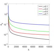
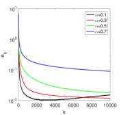
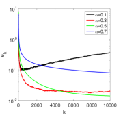
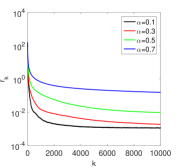
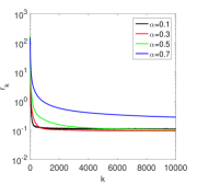
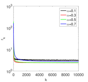
(a) $\delta=\text{1e-3}$	(b) $\delta=\text{1e-2}$	(c) $\delta=\text{5e-2}$

Figure 1: Numerical results for phillips with different noise levels by SGD (with various $\alpha$).

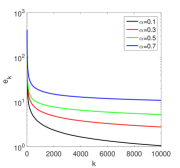
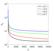
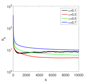
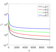
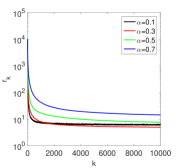
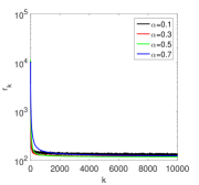
(a) $\delta=\text{1e-3}$	(b) $\delta=\text{1e-2}$	(c) $\delta=\text{5e-2}$

Figure 2: Numerical results for gravity with different noise levels by SGD (with various $\alpha$).

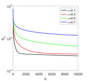
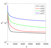
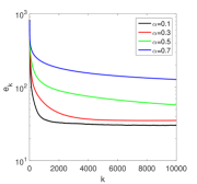
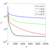
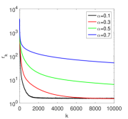
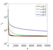
(a) $\delta=\text{1e-3}$	(b) $\delta=\text{1e-2}$	(c) $\delta=\text{5e-2}$

Figure 3: Numerical results for shaw with different noise levels by SGD (with various $\alpha$).

6.2 Comparison with Landweber method

Since SGD is a randomized version of the classical Landweber method, in Fig. 4, we compare their performance. To compare the iteration complexity only, we count one Landweber iteration as $n$ SGD iterations, and the full gradient evaluation is indicated by flat segments in the plots. For all examples, the error $e_{k}$ and residual $r_{k}$ first experience fast reduction, and then the error starts to increase, which is especially pronounced at $\delta=5\times 10^{-2}$, exhibiting the typical semiconvergence behavior. During the initial stage, SGD is much more effective than SGD: indeed one single loop over all the data can already significantly reduce the error $e_{k}$ and produce an acceptable approximation. The precise mechanism for this interesting observation will be further examined below. However, the nonvanishing variance of the stochastic gradient slows down the asymptotic convergence of SGD, and the error $e_{k}$ and the residual $r_{k}$ eventually tend to oscillate for noisy data, before finally diverge.

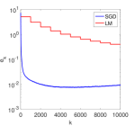
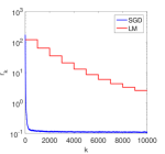
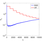
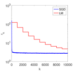
(a) phillips, $\delta=10^{-2}$	(b) phillips, $\delta=5\times 10^{-2}$
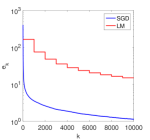
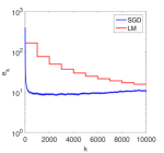
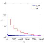
(c) gravity, $\delta=10^{-2}$	(d) gravity, $\delta=5\times 10^{-2}$
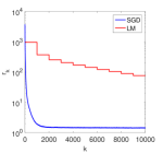
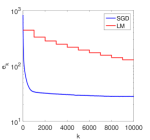
(e) shaw, $\delta=10^{-2}$	(f) shaw, $\delta=5\times 10^{-2}$

Figure 4: Numerical results for the examples by SGD (with $\alpha=0.1$) and LM.

6.3 Preasymptotic convergence

Now we examine the preasymptotic strong convergence of SGD (note that the weak error satisfies a Landweber type iteration). Theorem 2.4 (and Lemma 5.1) predicts that during first iterations, the low-frequency error $e_{L}:=\mathbb{E}[\|P_{\mathcal{L}}e_{k}\|^{2}]$ decreases rapidly, but the high-frequency error $e_{H}:=\mathbb{E}[\|P_{\mathcal{H}}e_{k}\|^{2}]$ can at best decay mildly. For all examples, the first five singular vectors can well capture the total energy of the initial error $e_{1}=x^{*}-x_{1}$, which suggests a truncation level $L=5$ for the numerical illustration. We plot the low- and high-frequency errors $e_{L}$ and $e_{H}$ and the total error $e=\mathbb{E}[\|e_{k}\|^{2}]$ in Fig. 5. The low-frequency error $e_{L}$ decays much more rapidly during the initial iterations, and since under the source condition (2.3), $e_{L}$ is indeed dominant, the total error $e$ also enjoys a fast initial decay. Intuitively, this behavior may be explained as follows. The rows of the matrix ${A}$ mainly contain low-frequency modes, and thus each SGD iteration tends to mostly remove the low-frequency component $e_{L}$ of the initial error $x^{*}-x_{1}$. The high-frequency component $e_{H}$ experiences a similar but much slower decay. Eventually, both components level off and oscillate, due to the deleterious effect of noise. These observations confirm the preasymptotic analysis in Section 5. For noisy data, the error $e_{k}$ can be highly oscillating, so is the residual $r_{k}$. The larger the noise level $\delta$ is, the larger the oscillation magnitude becomes.

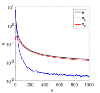
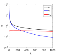
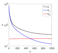
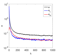
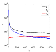
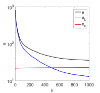
(a) phillips	(b) gravity	(c) shaw

Figure 5: The error decay for the examples with two noise levels: $\delta=10^{-2}$ (top) and $\delta=5\times 10^{-2}$ (bottom), with a truncation level $L=5$.

6.4 Asymptotic convergence

To examine the asymptotic convergence (with respect to the noise level $\delta$), in Table 1, we present the smallest error $e$ along the trajectory and the number of iterations to reach the error $e$ for several different noise levels. It is observed that for all three examples, the minimal error $e$ increases steadily with the noise level $\delta$, whereas also the required number of iterations decreases dramatically, which qualitatively agrees well with Remark 2.1. Thus, SGD is especially efficient in the regime of high noise level, for which one or two epochs can already give very good approximations, due to the fast preasymptotic convergence. This agrees with the common belief that SGD is most effective for finding an approximate solution that is not highly accurate. At low noise levels, shaw takes far more iterations to reach the smallest error. This might be attributed to the fact that the exponent $p$ in the source condition (2.3) for shaw is much smaller than that for phillips or gravity, since the low-frequency modes are less dominating, as roughly indicated by the red curves in Fig. 5. Interestingly, for all examples, the error $e$ undergoes sudden change when the noise level $\delta$ increases from 1e-2 to 3e-2. This might be related to the exponent $\alpha$ in the step size schedule, which probably should be adapted to the noise level $\delta$ in order to achieve optimal balance between the computational efficiency and statistical errors.

Table 1: The (minimal) expected error $e$ for the examples.

$\delta$	phillips	gravity	shaw
1e-3	(1.09e-3,7.92e4)	(3.22e-1,4.55e5)	(2.92e0,3.55e6)
5e-3	(3.23e-3,1.83e4)	(5.65e-1,6.19e4)	(3.21e0,1.95e6)
1e-2	(6.85e-3,3.09e3)	(6.21e-1,4.60e4)	(6.75e0,1.15e6)
3e-2	(4.74e-2,4.20e2)	(2.60e0, 6.50e3)	(3.50e1,7.80e3)
5e-2	(6.71e-2,1.09e3)	(6.32e0, 2.55e3)	(3.70e1,1.28e3)

7 Concluding remarks

In this work, we have analyzed the regularizing property of SGD for solving linear inverse problems, by extending properly deterministic inversion theory. The study indicates that with proper early stopping and suitable step size schedule, it is regularizing in the sense that iterates converge to the exact solution in the mean squared norm as the noise level tends to zero. Further, under the canonical source condition, we prove error estimates, which depend on the noise level and the schedule of step sizes. Further we analyzed the preasymptotic convergence behavior of SGD, and proved that the low-frequency error can decay much faster than high-frequency error. This allows explaining the fast initial convergence of SGD typically observed in practice. The findings are complemented by extensive numerical experiments.

There are many interesting questions related to stochastic iteration algorithms that deserve further research. One outstanding issue is stopping criterion, and rigorous yet computationally efficient criteria have to be developed. In practice, the performance of SGD can be sensitive to the exponent $\alpha$ in the step size schedule [20]. Promising strategies for overcoming the drawback include averaging [22] and variance reduction [14]. It is of much interest to analyze such schemes in the context of inverse problems, including nonlinear inverse problems and penalized variants.

Appendix A Elementary inequalities

In this appendix, we collect some useful inequalities. We begin with an estimate on the operator norm. This estimate is well known (see, e.g., [17]).

Lemma A.1.

For $j<k$, and any symmetric and positive semidefinite matrix $S$ and step sizes $\eta_{j}\in(0,\|S\|^{-1}]$ and $p\geq 0$, there holds

$$\|\prod_{i=j}^{k}(I-\eta_{i}S)S^{p}\|\leq\frac{p^{p}}{e^{p}(\sum_{i=j}^{k}\eta_{i})^{p}}.$$

Next we derive basic estimates on finite sums involving $\eta_{j}=c_{0}j^{-\alpha}$, with $c_{0}>0$ and $\alpha\in[0,1)$.

Lemma A.2.

For the choice $\eta_{j}=c_{0}j^{-\alpha}$, $\alpha\in[0,1)$ and $r\in[0,1]$, for any $1\leq j<k$, there holds

$$\sum_{i=1}^{k}\eta_{i} \geq(2^{1-\alpha}-1)(1-\alpha)^{-1}c_{0}k^{1-\alpha},$$ (A.1)

$$\sum_{j=1}^{k-1}\frac{\eta_{j}}{(\sum_{i=j+1}^{k}\eta_{i})^{r}} \leq\left\{\begin{array}[]{ll}c_{0}^{1-r}B(1-\alpha,1-r)k^{(1-r)(1-\alpha)},&r\in[0,1),\\ 2^{\alpha}((1-\alpha)^{-1}+\ln k)&r=1,\end{array}\right.$$ (A.4)

where $B(\cdot,\cdot)$ is the Beta function defined by $B(a,b)=\int_{0}^{1}s^{a-1}(1-s)^{b-1}\mathrm{d}s$ for any $a,b>0$.

Proof.

Since $\alpha\in[0,1)$, we have $c_{0}^{-1}\sum_{i=1}^{k}\eta_{i}\geq\int_{1}^{k+1}s^{-\alpha}\mathrm{d}s=(1-\alpha)^{-1}((k+1)^{1-\alpha}-1)\geq(1-\alpha)^{-1}(2^{1-\alpha}-1)k^{1-\alpha}$. This shows the estimate (A.1). Next, since $\eta_{i}\geq c_{0}k^{-\alpha}$, for any $i=j+1,\ldots,k$, we have

$$c_{0}^{-1}\sum_{i=j+1}^{k}\eta_{i}\geq k^{-\alpha}(k-j).$$ (A.5)

If $r\in[0,1)$, by changing variables and by the definition of the Beta function $B(\cdot,\cdot)$, we have

$$c_{0}^{r-1}\sum_{j=1}^{k-1}\frac{\eta_{j}}{(\sum_{i=j+1}^{k}\eta_{i})^{r}}\leq k^{r\alpha}\sum_{j=1}^{k-1}j^{-\alpha}(k-j)^{-r}$$

$$\leq k^{r\alpha}\int_{0}^{k}s^{-\alpha}(k-s)^{-r}\mathrm{d}s=B(1-\alpha,1-r)k^{(1-r)(1-\alpha)}.$$

For $r=1$, it can be derived directly

$$\sum_{j=1}^{k-1}\frac{\eta_{j}}{\sum_{i=j+1}^{k}\eta_{i}}\leq k^{\alpha}\sum_{j=1}^{[\frac{k}{2}]}j^{-\alpha}(k-j)^{-1}+k^{\alpha}\sum_{j=[\frac{k}{2}]+1}^{k-1}j^{-\alpha}(k-j)^{-1}$$

$$\leq 2k^{\alpha-1}\sum_{j=1}^{[\frac{k}{2}]}j^{-\alpha}+2^{\alpha}\sum_{j=[\frac{k}{2}]+1}^{k-1}(k-j)^{-1}.$$

Simple computation gives $\sum_{j=[\frac{k}{2}]+1}^{k-1}(k-j)^{-1}\leq\ln k$ and $\sum_{j=1}^{[\frac{k}{2}]}j^{-\alpha}\leq(1-\alpha)^{-1}(\frac{k}{2})^{1-\alpha}.$ Combining the last two estimates yields the estimate (A.4). ∎

The next result gives some further estimates.

Lemma A.3.

For $\eta_{j}=c_{0}j^{-\alpha}$, with $\alpha\in(0,1)$, $\beta\in[0,1]$, and $r\geq 0$, there hold

$$\sum_{j=1}^{[\frac{k}{2}]}\frac{\eta_{j}^{2}}{(\sum_{i=j+1}^{k}\eta_{i})^{r}}j^{-\beta} \leq c_{\alpha,\beta,r}k^{-r(1-\alpha)+\max(0,1-2\alpha-\beta)},$$

$$\sum_{j=[\frac{k}{2}]+1}^{k-1}\frac{\eta_{j}^{2}}{(\sum_{i=j+1}^{k}\eta_{i})^{r}}j^{-\beta} \leq c_{\alpha,\beta,r}^{\prime}k^{-((2-r)\alpha+\beta)+\max(0,1-r)},$$

where we slightly abuse $k^{-\max(0,0)}$ for $\ln k$, and the constants $c_{\alpha,\beta,r}$ and $c^{\prime}_{\alpha,\beta,r}$ are given by

$$c_{\alpha,\beta,r} =c_{0}^{2-r}\left\{\begin{array}[]{ll}2^{r}(2\alpha+\beta-1)^{-1},&2\alpha+\beta>1,\\ 2,&2\alpha+\beta=1,\\ 2^{r-1+2\alpha+\beta}(1-2\alpha-\beta)^{-1},&2\alpha+\beta<1,\end{array}\right.$$

$$c^{\prime}_{\alpha,\beta,r} =2^{2\alpha+\beta}c_{0}^{2-r}\left\{\begin{array}[]{ll}(r-1)^{-1},&r>1,\\ 1,&r=1,\\ 2^{r-1}(1-r)^{-1},&r<1.\end{array}\right.$$

Proof.

It follows from the inequality (A.5) that

$$\quad c_{0}^{r-2}\sum_{j=1}^{[\frac{k}{2}]}\frac{\eta_{j}^{2}}{(\sum_{i=j+1}^{k}\eta_{i})^{r}}j^{-\beta}=\sum_{j=1}^{[\frac{k}{2}]}\frac{j^{-(2\alpha+\beta)}}{(\sum_{i=j+1}^{k}i^{-\alpha})^{r}}$$

$$\leq k^{r\alpha}\sum_{j=1}^{[\frac{k}{2}]}j^{-(2\alpha+\beta)}(k-j)^{-r}\leq 2^{r}k^{-r+r\alpha}\sum_{j=1}^{[\frac{k}{2}]}j^{-(2\alpha+\beta)}$$

$$\leq 2^{r}k^{r\alpha-r}\left\{\begin{array}[]{ll}(2\alpha+\beta-1)^{-1},&2\alpha+\beta>1,\\ \ln k,&2\alpha+\beta=1,\\ (1-2\alpha-\beta)^{-1}(\frac{k}{2})^{1-2\alpha-\beta},&2\alpha+\beta<1.\end{array}\right.$$

Collecting terms shows the first estimate. The second estimate follows similarly. ∎

Last, we give a technical lemma on recursive sequences.

Lemma A.4.

Let $\eta_{j}=c_{0}j^{-\alpha}$, $\alpha\in(0,1)$. Given $\{b_{j}\}_{j=1}^{\infty}\subset\mathbb{R}_{+}$, $a_{1}\geq 0$ and $c_{i}>0$, $\{a_{j}\}_{j=2}^{\infty}\subset\mathbb{R}_{+}$ satisfies

$$a_{k+1}=c_{1}\sum_{j=1}^{k-1}\frac{\eta_{j}^{2}}{\sum_{i=j+1}^{k}\eta_{i}}a_{j}+c_{2}k^{-2\alpha}a_{k}+b_{k}.$$

If $b_{j}$ is nondecreasing, then for some $c(\alpha,c_{i})$ dependent of $\alpha$ and $c_{i}$, there holds

$$a_{k+1}\leq c(\alpha,c_{i})k^{-\min(\alpha,1-\alpha)}\ln k+2b_{k}.$$

Proof.

Let $c_{\alpha}=c(\alpha,0,1)+c^{\prime}(\alpha,0,1)$ from Lemma A.3. Take $k_{*}\in\mathbb{N}$ such that $c_{1}c_{\alpha}k^{-\min(1-\alpha,\alpha)}\ln k+c_{2}k^{-2\alpha}<1/2$ for any $k\geq k_{*}$. The existence of a finite $k_{*}$ is due to the monotonicity of $f(t)=t^{-\min(1-\alpha,\alpha)}\ln t$ for large $t>0$ and $\lim_{t\to\infty}f(t)=0$. Now we claim that there exists $a_{*}>0$ such that $a_{k}\leq a_{*}+2b_{k}$ for any $k\in\mathbb{N}.$ Let $a_{*}=\max_{1\leq k\leq k_{*}}a_{k}$. The claim is trivial for $k\leq k_{*}$. Suppose it holds for some $k\geq k_{*}$. Then by Lemma A.3 and the monotonicity of $b_{j}$,

$$a_{k+1} \leq\max_{1\leq i\leq k}a_{i}\Big{(}c_{1}\sum_{j=1}^{k-1}\frac{\eta_{j}^{2}}{\sum_{i=j+1}^{k}\eta_{i}}+c_{2}k^{-2\alpha}\Big{)}+b_{k}$$

$$\leq(a_{*}+2b_{k})(c_{1}c_{\alpha}k^{-\min(\alpha,1-\alpha)}\ln k+c_{2}k^{-2\alpha})+b_{k}$$

$$\leq\tfrac{1}{2}(a_{*}+2b_{k})+b_{k}\leq a_{*}+2b_{k+1},$$

This shows the claim by mathematical induction. Next, by Lemma A.3, for any $k>k_{*}$, we have

$$a_{k+1} \leq(a_{*}+2b_{k})(c_{1}c_{\alpha}k^{-\min(\alpha,1-\alpha)}\ln k+c_{2}k^{-2\alpha})+b_{k}$$

$$\leq c(\alpha,c_{i})k^{-\min(\alpha,1-\alpha)}\ln k+2b_{k}.$$

This completes the proof of the lemma. ∎

Remark A.1.

By the argument in Lemma A.4 and a standard bootstrapping argument, we deduce the following assertions. If $\sup_{j}b_{j}<\infty$, then $\{a_{j}\}_{j=1}^{\infty}$ is bounded by a constant dependent of $\alpha$, $\sup_{j}b_{j}$ and $c_{i}$s. Further, if $b_{j}\leq c_{3}j^{-\gamma}$, $j\in\mathbb{N}$ with $\gamma>0$, then for some $c(\alpha,\gamma,c_{i},\ell)$ dependent of $\alpha$, $\gamma$, $\ell$ and $c_{i}$s, there holds

$$a_{k+1}\leq c(\alpha,\gamma,c_{i},\ell)k^{-\min(\ell\alpha,1-\alpha,\gamma)}\ln^{\ell}k.$$

References

- [1] F. Bauer, T. Hohage, and A. Munk. Iteratively regularized Gauss-Newton method for nonlinear inverse problems with random noise. SIAM J. Numer. Anal., 47(3):1827–1846, 2009.
- [2] N. Bissantz, T. Hohage, and A. Munk. Consistency and rates of convergence of nonlinear Tikhonov regularization with random noise. Inverse Problems, 20(6):1773–1789, 2004.
- [3] N. Bissantz, T. Hohage, A. Munk, and F. Ruymgaart. Convergence rates of general regularization methods for statistical inverse problems and applications. SIAM J. Numer. Anal., 45(6):2610–2636, 2007.
- [4] L. Bottou. Large-scale machine learning with stochastic gradient descent. In Y. Lechevallier and G. Saporta, editors, Proc. CompStat’2010, pages 177–186. Springer, Heidelberg, 2010.
- [5] L. Bottou, F. E. Curtis, and J. Nocedal. Optimization methods for large-scale machine learning. SIAM Rev., 60(2):223–311, 2018.
- [6] K. Chen, Q. Li, and J.-G. Liu. Online learning in optical tomography: a stochastic approach. Inverse Problems, 34(7):075010, 26 pp., 2018.
- [7] A. Dieuleveut and F. Bach. Nonparametric stochastic approximation with large step-sizes. Ann. Statist., 44(4):1363–1399, 2016.
- [8] H. W. Engl, M. Hanke, and A. Neubauer. Regularization of Inverse Problems. Kluwer, Dordrecht, 1996.
- [9] K. Ito and B. Jin. Inverse Problems: Tikhonov Theory and Algorithms. World Scientific, Hackensack, NJ, 2015.
- [10] S. Jastrzȩbski, Z. Kenton, D. Arpit, N. Ballas, A. Fischer, Y. Bengio, and A. Storkey. Three factors influencing minima in SGD. Preprint, arXiv:1711.04623, 2017.
- [11] N. Jia and E. Y. Lam. Machine learning for inverse lithography: using stochastic gradient descent for robust photomask synthesis. J. Opt., 12(4):045601, 9 pp., 2010.
- [12] Y. Jiao, B. Jin, and X. Lu. Preasymptotic convergence of randomized Kaczmarz method. Inverse Problems, 33(12):125012, 21 pp., 2017.
- [13] B. Jin and D. A. Lorenz. Heuristic parameter-choice rules for convex variational regularization based on error estimates. SIAM J. Numer. Anal., 48(3):1208–1229, 2010.
- [14] R. Johnson and T. Zhang. Accelerating stochastic gradient descent using predictive variance reduction. In C. J. C. Burges, L. Bottou, M. Welling, Z. Ghahramani, and K. Q. Weinberger, editors, NIPS’13, pages 315–323, Lake Tahoe, Nevada, 2013.
- [15] B. Kaltenbacher, A. Neubauer, and O. Scherzer. Iterative Regularization Methods for Nonlinear Ill-posed Problems. Walter de Gruyter, Berlin, 2008.
- [16] Q. Li, C. Tai, and W. E. Dynamics of stochastic gradient algorithms. Preprint, arXiv:1511.06251v2 (last accessed on July 5, 2018), 2015.
- [17] J. Lin and L. Rosasco. Optimal rates for multi-pass stochastic gradient methods. J. Mach. Learn. Res., 18:1–47, 2017.
- [18] F. Natterer. The Mathematics of Computerized Tomography. SIAM, Philadelphia, PA, 2001.
- [19] D. Needell, N. Srebro, and R. Ward. Stochastic gradient descent, weighted sampling, and the randomized Kaczmarz algorithm. Math. Program., 155(1-2, Ser. A):549–573, 2016.
- [20] A. Nemirovski, A. Juditsky, G. Lan, and A. Shapiro. Robust stochastic approximation approach to stochastic programming. SIAM J. Optim., 19(4):1574–1609, 2008.
- [21] S. Pereverzev and E. Schock. On the adaptive selection of the parameter in regularization of ill-posed problems. SIAM J. Numer. Anal., 43(5):2060–2076, 2005.
- [22] B. T. Polyak and A. B. Juditsky. Acceleration of stochastic approximation by averaging. SIAM J. Control Optim., 30(4):838–855, 1992.
- [23] H. Robbins and S. Monro. A stochastic approximation method. Ann. Math. Stat., 22:400–407, 1951.
- [24] N. Shirish Keskar, D. Mudigere, J. Nocedal, M. Smelyanskiy, and P. T. P. Tang. On large-batch training for deep learning: generalization gap and sharp minima. In Proc. ICLR, page arXiv:1609.04836. 2017.
- [25] T. Strohmer and R. Vershynin. A randomized Kaczmarz algorithm with exponential convergence. J. Fourier Anal. Appl., 15(2):262–278, 2009.
- [26] P. Tarrès and Y. Yao. Online learning as stochastic approximation of regularization paths: optimality and almost-sure convergence. IEEE Trans. Inform. Theory, 60(9):5716–5735, 2014.
- [27] Y. Ying and M. Pontil. Online gradient descent learning algorithms. Found. Comput. Math., 8(5):561–596, 2008.
- [28] Z. Zhu, J. Wu, B. Yu, L. Wu, and J. Ma. The anisotropic noise in stochastic gradient descent: its behavior of escaping from minima and regularization effects. Preprint, arXiv:1803.00195v2 (last accessed on July 5, 2018), 2018.