Image-processing the topological charge density in the ${\mathbb{C}P^{N-1}}$ model

Abstract

We study the topological charge density distribution using the two-dimensional ${\mathbb{C}P^{N-1}}$ model. We numerically compute not only the topological susceptibility, which is a spatially global quantity to probe topological properties of the whole system, but also the topological charge correlator with finite momentum. We perform Fourier power spectrum analysis for the topological charge density for various values of the inverse temperature $\beta$. We propose to utilize the Fourier entropy as a convenient measure to characterize spatial distribution patterns and demonstrate that the Fourier entropy exhibits nontrivial temperature dependence. We also consider the snapshot entropy defined with the singular value decomposition, which also turns out to behave nonmonotonically with the temperature. We give a possible interpretation suggested from the strong-coupling analysis.

I Introduction

Gauge topology is a fundamental aspect of modern field theory. It would be an ideal setup for theoretical investigations if a system is simple but still nontrivial enough to accommodate nonvanishing topological winding. The two-dimensional ${\mathbb{C}P^{N-1}}$ model is one of such ideal theoretical laboratories. The ${\mathbb{C}P^{N-1}}$ model has the asymptotic freedom, the linear confining potential, and instantons D’Adda et al. (1978); Di Vecchia et al. (1981); Duane and Green (1981); Kunz and Zumbach (1989). In fact, even on the analytical level, the dynamical mass generation and the linear confining potential have been derived in the large-$N$ expansion Witten (1979); Campostrini and Rossi (1992) as well as in the strong coupling expansion Samuel (1983); Plefka and Samuel (1997).

The ${\mathbb{C}P^{N-1}}$ model has a wide range of applications. Recently it is a hot and growing area to investigate “resurgence” using the ${\mathbb{C}P^{N-1}}$ model, that is, perturbative expandability and cancellation of ambiguity in each topological sector are intensely studied Dunne and Unsal (2012); Misumi et al. (2014); Fujimori et al. (2016). Also, we note that the ${\mathbb{C}P^{N-1}}$ model has plenty of connections to condensed matter physics systems. There are several equivalent formulations of the ${\mathbb{C}P^{N-1}}$ model such as SU($N$) Heisenberg ferromagnets, the tensor network with three-dimensional loop model which is generalized to the form of the tensor renormalization group, and so on Kataoka et al. (2011); Nahum et al. (2011, 2013); Kawauchi and Takeda (2016a, b); Takashima et al. (2006); Roy and Quella (2015). In particular, in Heisenberg spin systems, the ${\mathbb{C}P^{N-1}}$ model is relevant for a critical phase between the valence-bond solid and the antiferromagnetic phase Motrunich and Vishwanath (2008); Sandvik (2010). Furthermore, we point out that recent developments of condensed matter physics experiments has enabled us to emulate the ${\mathbb{C}P^{N-1}}$ model and its variants on the optical lattice Laflamme et al. (2016). In this way, although the ${\mathbb{C}P^{N-1}}$ is a relatively simple and well-established model, many interesting studies are ongoing to the present date.

From the point of view of gauge topology, which is of our present interest, the ${\mathbb{C}P^{N-1}}$ model has a prominent feature that the topological charge can be defined geometrically Berg and Luscher (1981) and it rigorously takes integer values even on the lattice. There are several subtle points, however. Even with rigorous quantization, the physical interpretation in terms of instantons may become unclear in some parameter regions. When the temperature or the coupling constant is far away from the region corresponding to the continuum limit, the physical lattice spacing would be too coarse to hold the instantons on the lattice. For further discussions on lattice artifacts such as finite size effects and the critical slowing down of topological sectors, see Refs. Rossi and Vicari (1993); Irving and Michael (1992); Rossi and Vicari (1993); Del Debbio et al. (2004) for example. Also, in the region with small $N$, quantum fluctuations would melt instantons by blurring them into quasi-particles. Therefore, we can perform the instanton gas analysis at large $N$, while melting instantons causes the precocious scaling in small-$N$ regions Andersen et al. (2006); Lian and Thacker (2007); Diakonov and Maul (2000); Maul et al. (2000). Nevertheless, regardless of the physical interpretation, the topological winding anyway exists in theory for any parameters, and it would be desirable to perform analysis on the winding not necessarily in an intuitive picture of instantons.

The ${\mathbb{C}P^{N-1}}$ model is an intriguing lattice model on its own, and additionally, one of important model usages is to adopt it as a toy model for more complicated theories such as QCD-like theories, where QCD stands for quantum chromodynamics. Historically speaking, the instantons and the $\theta$-vacuum were first revealed for QCD in the context to understand color confinement and spontaneous and anomalous chiral symmetry breaking. It has been a widely accepted idea that the chiral condensate that spontaneously breaks chiral symmetry is induced by fermionic zeromodes associated with the instanton gauge background Diakonov and Petrov (1984) (see Ref. Schäfer and Shuryak (1998) for a comprehensive review). Also, recently, there are significant progresses in theoretical studies of color confinement based on the instanton with nontrivial holonomy (see, for example, a proceedings article in Ref. Shuryak (2017) and references therein, and also Ref. Fukushima and Skokov (2017) for a recent review).

Now, it is still a challenging problem how to access topologically nontrivial sectors generally in field theories. This is the case also for simple models such as the ${\mathbb{C}P^{N-1}}$ model. For this purpose to study topological contents, the topological susceptibility, $\chi_{t}$, is the most common observable to quantify fluctuations with respect to the topological charge. Roughly speaking, if $\chi_{t}$ is large, the system should accommodate more instantons which enhance nonperturbative effects. There are a countless number of precedent works on physics implications of $\chi_{t}$ in various theories including QCD (see Refs. Borsanyi et al. (2016); Kitano and Yamada (2015) for recent attempts motivated with axion cosmology and Ref. Marsh (2016) for a review). For more phenomenological applications of the topological susceptibility and related observables in hadron physics, see a lecture note in Ref. Shore (2008).

Since topological excitations are inherently nonperturbative, the information available from analytical considerations is limited, and the numerical Monte-Carlo simulation on the lattice is the most powerful approach Alles et al. (1997a); *Alles:1997sy; *Alles:2004vi. For the ${\mathbb{C}P^{N-1}}$ model, there are many lattice studies Duane and Green (1981); Kunz and Zumbach (1989); Campostrini et al. (1992); Hasenbusch and Meyer (1993). We shall make a remark that the ${\mathbb{C}P^{N-1}}$ model action has a special analytical structure such that the sign problem is tamed even with a nonzero chemical potential Rindlisbacher and de Forcrand (2017); Evans et al. (2016) or a $\theta$ term Burkhalter et al. (2001); Azcoiti et al. (2004); Beard et al. (2005); Imachi et al. (2005); Kawauchi and Takeda (2016b), which is an advantage over other complicated systems.

In this paper we revisit the topological properties in the ${\mathbb{C}P^{N-1}}$ model. For actual procedures we will regard the two-dimensional field configurations in the ${\mathbb{C}P^{N-1}}$ model as “image” data and will “image-process” the distribution of the topological charge density at various temperatures. Our motivation partly comes from an analogy to finite-temperature QCD in which $\chi_{t}$ changes with temperature. Actually, we do not restrict our ${\mathbb{C}P^{N-1}}$ model temperature to the scaling region near the continuum limit; the ${\mathbb{C}P^{N-1}}$ model is anyway a well-defined lattice theory for any temperature. (We will never discuss practical applicability to QCD and the continuum limit in the present study.)

As a first step, we perform the Fourier power spectrum analysis of the topological charge density. This power spectrum amounts to a momentum dependent generalization of the topological susceptibility, which has been discussed and partially measured also in QCD in Refs. Shore (1998); Fukushima et al. (2001); Koma et al. (2010). The entire structures of the correlator in momentum space are quite informative, as we will reveal in this work, but such calculations are too much resource consuming. Therefore, it would be much more convenient if there is any single measure extracting essential features of the topological charge density distribution as a function of temperature. We will propose to use an entropy defined with the Fourier spectrum. Also, another observable is obtained to make use of the singular value decomposition (SVD) of the image data. As a standard image-processing tool, the SVD is commonly employed; see Refs. Matsueda (2012); Matsueda and Ozaki (2015); Lee et al. (2015) for physics applications of the SVD to image-process the spin configurations. In the same way as in the Fourier power spectrum analysis, interestingly, an entropy is constructed with the SVD eigenvalues, which will be referred to as the “snapshot entropy,” which will turn out to have nontrivial temperature dependence.

This paper is organized as follows. In Sec. II we will review the ${\mathbb{C}P^{N-1}}$ model and the simulation algorithm. We will introduce physical observables including the Fourier and the snapshot entropies in Secs. II.2 and II.3. Section III is devoted to the numerical setups and the consistency checks with the precedent lattice simulation results. In Sec. V we will report our main numerical results, namely, the Fourier power spectrum analysis of the topological charge correlator in Sec. V.1, the Fourier and the snapshot entropies in Secs. V.2 and V.3, and their correlations in Sec. V.4. For a possible interpretation of transitional behavior we will discuss phase boundaries between confinement and infinitesimal deconfinement from the strong-coupling character expansion. Finally, in Sec. VII, we will make conclusions and outlook.

II Formulation

We will make a brief overview of the numerical lattice simulation in the ${\mathbb{C}P^{N-1}}$ model. We adopt the method formulated in Ref. Campostrini et al. (1992) to compute physical observables. We will also give an explanation of unconventional observables called the Fourier entropy and the snapshot entropy.

II.1 ${\mathbb{C}P^{N-1}}$ Model and the Monte-Carlo Method

The ${\mathbb{C}P^{N-1}}$ model is defined by the following partition function,

$$Z=\int\mathcal{D}z\,\mathcal{D}\lambda\,\prod_{x}\delta(|z(x)|^{2}-1)\,e^{-\beta H}$$ (1)

with the Hamiltonian,

$$H=-N\sum_{x,\mu}\bigl{[}\bar{z}(x+\hat{\mu})z(x)\lambda_{\mu}(x)+\text{(c.c.)}-2\bigr{]}\,,$$ (2)

where $z(x)$ represents complex scalar fields with $N$ components which are constrained as $|z(x)|^{2}=1$, and (c.c.) is the complex conjugate of the first term. The symbol $\hat{\mu}$ denotes the unit lattice vector. Since there is no kinetic term, $\lambda_{\mu}(x)$ is an auxiliary U(1) link variable. We will refer to $\beta$ as the (inverse) temperature throughout this paper. In some literature $g\equiv 1/(N\beta)$ is often introduced as a “coupling constant” but we will consistently use the inverse temperature $\beta$ only.

The Monte-Carlo simulation consists of two procedures called “update” and “step” which are explained respectively below. For one update we randomly choose a point $x$, and calculate new $z(x)$ and $\lambda_{\mu}(x)$ at this point $x$ according to the probability distributions, which will be explicitly given in the subsequent paragraphs. One step has $L^{2}$ updates, where $L$ is the lattice size.

To make this paper self-contained, let us elucidate how to update $z(x)$ at a chosen $x$. We can update $\lambda_{\mu}(x)$ similarly. According to a method called the “over–heat bath method” in Ref. Campostrini et al. (1992) we successively update the configurations. It is important that we can write the $z(x)$-dependent piece of the Hamiltonian as

$$H=-N\langle z(x),F_{z}(x)\rangle+\cdots\,,$$ (3)

where the ellipsis represents terms not involving $z(x)$. In the above we introduced the inner product of the $N$ component scalar fields defined by $\langle a,b\rangle\equiv\mathrm{Re}\,\sum_{i}\bar{a}_{i}b_{i}$. We can easily infer

$$F_{z}(x)=\sum_{\mu}\bigl{[}z(x-\hat{\mu})\lambda_{\mu}(x-\hat{\mu})+z(x+\hat{\mu})\bar{\lambda}_{\mu}(x)\bigr{]}$$ (4)

from the Hamiltonian. The inner product of the $N$ component complex scalars can be regarded as that of the $2N$ component real scalars, i.e., $\langle a,b\rangle=\sum_{i}(\mathrm{Re}\,a_{i}\mathrm{Re}\,b_{i}+\mathrm{Im}\,a_{i}\mathrm{Im}\,b_{i})$. Then, for this real inner product, we can define the relative angle $\theta$ as

$$\langle z(x),F_{z}(x)\rangle=|F_{z}(x)|\cos\theta(x)\,.$$ (5)

Here we used $|z(x)|=1$. Because the above form depends only on the relative angle $\theta(x)$, the choice of $z(x)$ is not yet unique for the same $\langle z(x),F_{z}(x)\rangle$. The over–heat bath method fixes new $z(x)$ uniquely in such a way to disturb the system maximally.

For the update we first sample a new angle $\theta$ (that is denoted as $\theta^{\rm new}$ below) according to the probability,

$$dp_{N}(\theta)\propto d\theta\,(\sin\theta)^{2N-2}e^{\beta N|F_{z}|\cos\theta}\,,$$ (6)

where $(\sin\theta)^{2N-2}$ appears from the measure given by the surface area of sphere in $2N$-dimensional space.

We next specify new $z(x)$ [that is denoted as $z^{\rm new}(x)$ below] with chosen $\theta^{\rm new}$. In the over–heat bath method, we take $z^{\rm new}(x)$ to minimize an overlap with original $z(x)$, that is, $\langle z^{\rm new}(x),z(x)\rangle$ is minimized. This can be achieved with

$$z^{\rm new}=\cos\theta^{\rm new}\frac{F_{z}}{|F_{z}|}-\biggl{(}z-\cos\theta\frac{F_{z}}{|F_{z}|}\biggr{)}\frac{\sin\theta^{\rm new}}{\sin\theta}\,.$$ (7)

After doing this for $z(x)$, for the same $x$, we perform the update, $\lambda_{\mu}(x)\,\to\,\lambda_{\mu}^{\rm new}(x)$, in the same way.

II.2 Physical Observables

In this work we measure physical observables in units of the lattice spacing $a$. This means that $\beta$-dependence may enter through the running coupling $\beta(a)$. If necessary, we could convert observables in the physical unit with a typical length scale, i.e. correlation length, though we won’t.

The energy density is one of the most elementary physical observables, that is given by

$$E=\frac{1}{2NV}\langle H\rangle$$ (8)

with the dimensionless volume $V\equiv L^{2}$. It is useful to keep track of $E$ to monitor if the numerical simulation converges properly.

We shall define the correlation length. The U(1) invariance implies that the basic building block of local physical observables should be the following local operator (that is, a counterpart of a mesonic state in lattice QCD language),

$$P_{ij}(x)=\bar{z}_{i}(x)z_{j}(x)\,.$$ (9)

The two-point correlation of $P_{ij}(x)$ is

$$G_{P}(x,y)=\langle{\rm tr}P(x)P(y)\rangle-\frac{1}{N}\,,$$ (10)

where the last term $1/N$ subtracts the disconnected part. In the perturbative regime near the scaling region, the correlation function in momentum space is expected to scale as

$$\tilde{G}_{P}(k)\sim\frac{Z_{P}}{\xi_{G}^{-2}+\sum_{\mu}4\sin^{2}(k_{\mu}/2)}\,,$$ (11)

where $k_{\mu}$ is discretized as $k_{\mu}=2\pi n_{\mu}/L$ with $n_{\mu}=0,1,2,\dots,L-1$ for the lattice size $L$ (where we use a notation slightly different from Ref. Campostrini et al. (1992)). We note that the above form assumes the periodic boundary condition at the spatial edges. Using the smallest nonzero momentum $k_{(1,0)}\equiv(2\pi/L,0)$, we can solve the correlation length as

$$\xi_{G}^{2}=\frac{1}{4\sin^{2}(\pi/L)}\biggl{[}\frac{\tilde{G}_{P}(0)}{\tilde{G}_{P}(k_{(1,0)})}-1\biggr{]}\,.$$ (12)

as given in Ref. Campostrini et al. (1992). As we mentioned in the beginning of this section, dimensionful observables must scale with physical $\xi_{G}$ in the scaling region as this is the only scaling factor. For example, in the scaling region in the large-$N$ expansion, the analytical behavior is known as Campostrini and Rossi (1992)

$$\frac{\beta^{2}\tilde{G}_{P}(0)}{\xi_{G}^{2}}=\frac{3}{2\pi}+O(N^{-1})\,.$$ (13)

Our central interest in this work lies in the topological properties of the theory. Here, we adopt the following geometrical definition of the topological charge density,

$$\begin{split}\rho(x)&\equiv\frac{1}{2\pi}\Bigl{\{}\arg\bigl{[}{\rm tr}P(x+\hat{1}+\hat{2})P(x+\hat{1})P(x)\bigr{]}\\ &\qquad+\arg\bigl{[}{\rm tr}P(x+\hat{2})P(x+\hat{1}+\hat{2})P(x)\bigr{]}\Bigr{\}}\,,\end{split}$$ (14)

where $\arg$ denotes the principal value of the complex argument within the interval $(-\pi,\pi]$. Then the quantized topological charge is

$$Q=\sum_{x}\rho(x)\,.$$ (15)

It is mathematically proven that this $Q$ rigorously takes integer values even on discretized lattice, which is a preferable advantage to use the ${\mathbb{C}P^{N-1}}$ model.

Using $Q$ as constructed above, we can define the topological susceptibility as

$$\chi_{t}\equiv\sum_{x}\langle\rho(x)\rho(0)\rangle=\frac{1}{V}\bigl{(}\langle Q^{2}\rangle-\langle Q\rangle^{2}\bigr{)}\,.$$ (16)

In the large-$N$ expansion the analytical behavior of the topological susceptibility is known as well. That is, in the leading order of the large-$N$ expansion, the topological susceptibility obtains as

$$\chi_{t}=\frac{3m_{0}^{2}}{\pi N}+O(N^{-2})\,,$$ (17)

where $m_{0}$ is the vacuum expectation value of an auxiliary field which gives a dynamical mass for $z(x)$. In terms of the momentum cutoff $M_{\rm cut}$, it can be expressed as

$$m_{0}^{2}=M_{\rm cut}^{2}e^{-4\pi\beta}\,,$$ (18)

which leads to the following expression D’Adda et al. (1978),

$$\chi_{t}(\beta)=\frac{3M_{\rm cut}^{2}}{\pi N}e^{-4\pi\beta}+O(N^{-2})$$ (19)

as a function of $\beta$ at the one-loop level. We can also express this using $\beta$-dependent $\xi_{G}$ whose leading form is Campostrini and Rossi (1992)

$$\xi_{G}^{2}=\frac{1}{6m_{0}^{2}}+O(N^{-2})=\frac{1}{6M_{\rm cut}^{2}}e^{4\pi\beta}+O(N^{-2})\,.$$ (20)

The leading behavior of $\chi_{t}$ is thus characterized as

$$\chi_{t}\,\xi_{G}^{2}=\frac{1}{2\pi N}+O(N^{-2})$$ (21)

in the scaling region, but this scaling relation does not hold for not large enough $N$ or $\beta$.

II.3 Fourier and Snapshot Entropies

In this paper we will pay our special attention to the Fourier entropy and the snapshot entropy defined by spatial distribution of $\rho(x)$, which will be useful for our image-processing purpose.

We shall introduce the Fourier entropy as the Shannon entropy using the Fourier transformed topological charge density, $\tilde{\rho}(k)$. The normalization convention of discrete Fourier transform (DFT) is chosen as

$$\tilde{\rho}(k)=\frac{1}{\sqrt{V}}\sum_{x^{\mu}}e^{-ik\cdot x}\rho(x)\,,$$ (22)

where $x^{\mu}$ runs over $0,\dots,L-1$ in units of $a=1$. We first define the normalized Fourier spectrum as

$$f_{\rm DFT}(k)\equiv\frac{|\tilde{\rho}(k)|^{2}}{\sum_{k^{\prime}}|\tilde{\rho}(k^{\prime})|^{2}}\,,$$ (23)

and then the Fourier entropy reads,

$$S_{\rm DFT}\equiv-\sum_{k}f_{\rm DFT}(k)\ln f_{\rm DFT}(k)\,.$$ (24)

The entropy quantifies how the topological charge density distributes over space. For $k$-independent constant $\tilde{\rho}$, $S_{\rm DFT}$ is saturated at $2\ln L$.

Another quantity which reflects the spatial pattern of $\rho(x)$ is the snapshot entropy defined with the singular values. Although our numerical simulation in the present work uses the square lattice, the procedure is applicable for general rectangular lattices. On the lattice the image of the topological charge density is regarded as an $L\times L$ real-valued matrix, and its SVD for $x=(x_{1},x_{2})$ is written as

$$\rho(x_{1},x_{2})=\sum_{n=1}^{L}\lambda^{(n)}U^{(n)}_{x_{1}}V^{(n)}_{x_{2}}\,.$$ (25)

Here, $U^{(n)}$ and $V^{(n)}$ are two sets of orthonormal bases in $L$-dimensional vector space given by diagonalizing the matrix $\rho^{{\dagger}}\rho$. Singular values, $\lambda^{(n)}$, sorted in descending order are given by the square root of the eigenvalue of $\rho^{{\dagger}}\rho$. The two-dimensional image of $U^{(n)}_{x_{1}}V^{(n)}_{x_{2}}$ is referred to as the $n$-th SVD layer, and the weight for each SVD layer is $\lambda^{(n)}$. Because all $\lambda^{(n)}$’s are nonnegative by construction, we can define the snapshot entropy as the Shannon entropy using $\lambda^{(n)}$. For this purpose we first normalize the singular values as

$$f_{\rm SVD}(n)\equiv\frac{\lambda^{(n)}}{\sum_{n^{\prime}}\lambda^{(n^{\prime})}}\,,$$ (26)

and then the snapshot entropy reads,

$$S_{\rm SVD}\equiv-\sum_{n=1}^{L}f_{\rm SVD}(n)\ln f_{\rm SVD}(n)\,.$$ (27)

The maximum value of $S_{\rm SVD}$ is $\ln L$.

III Simulation Setups and Consistency Checks

We here detail our numerical simulation processes. We have performed the calculations for $N=2$, $3$, $10$, $21$ with the $L=32$ lattice size to see the $N$ dependence, and for $N=10$ with $L=32$, $64$, and $128$ lattice sizes to see the $L$ dependence.

For each combination of $(N,L)$, we have initialized the configuration with the random start (i.e., hot start), and we have confirmed that thermalization is achieved by 2000 Monte-Carlo steps; we have checked this by comparing results in the hot and the cold starts. After thermalization we take 1000 sampling points with an interval by 100 steps to measure physical observables. For the error estimate of physical observables we use the standard Jack-knife method with $\text{(bin width)}=10$. We have chosen the bin width and the interval to suppress the autocorrelation which is checked by the error estimate of the energy density at several $(N,L)$. Our simulation starts with $\beta=0.1$ and we increase $\beta$ by $0.1$ until $\beta=1.5$, and for each $\beta$ we repeat the above procedures.

We have quantitatively checked the full consistency of our results and previous results in Ref. Campostrini et al. (1992) for the energy density $E$, the correlation length $\xi_{G}^{2}$, and the topological susceptibility $\chi_{t}$ at several same $(N,L)$, as listed in Tab. 1. In this table, our error estimations include only the statistical error from the Monte-Carlo simulation. In principle, $\xi_{G}^{2}$ might contain additional errors from prescription of subtracting the disconnected part of the correlation function in Eq. (10).

Our Results
($N,\,L$)	$\beta$	$E$	$\xi_{G}^{2}$	$\chi_{t}$
(2, 36)	1.1	0.556245(80)	12.6(1.7)	0.008083(85)
(10, 42)	0.7	0.784321(44)	5.05(55)	0.004997(49)
(10, 30)	0.8	0.666134(52)	24.26(31)	0.000827(94)
(10, 60)	0.8	0.667047(26)	21.2(1.1)	0.000999(10)
(21, 36)	0.7	0.738992(32)	14.25(20)	0.0005513(81)
Previous Results
($N,\,L$)	$\beta$	$E$	$\xi_{G}^{2}$	$\chi_{t}$
(2, 36)	1.1	0.55593(14)	12.11(48)	—
(10, 42)	0.7	0.78402(13)	5.52(14)	0.00505(11)
(10, 30)	0.8	0.66591(17)	25.70(40)	—
(10, 60)	0.8	0.66701(8)	21.80(47)	0.00101(4)
(21, 36)	0.7	0.73888(15)	14.66(22)	—

Table 1: Comparison of our results and previous results in Ref. Campostrini et al. (1992) for various $(N,L)$ and $\beta$. In order to establish the consistency, we have collected $2\times 10^{4}$ statistics with Jack-knife width $10$ for our results.

Now, let us proceed to more detailed numerical results for respective physical observables. Figure 1 shows the energy density $E$ as a function of $\beta$ for $N=10$ and $L=32$, $64$, $128$. We note that this $E$ is a bare one measured in units of the lattice spacing $a$, and thus a part of $\beta$-dependence is attributed to $\beta(a)$ as we pointed out. We make this plot just to see the volume dependence, and it is clear from Fig. 1 that the volume dependence is negligibly small within the error bars. Actually, $L=32$ is already sufficiently close to the thermodynamic limit. We can understand this from the correlation length shown in Fig. 2. As long as $\beta$ is not too large, the correlation length is significantly smaller than the lattice size $L=32$ for any $N$, so that the finite size artifact is expected to be small already for $L=32$.

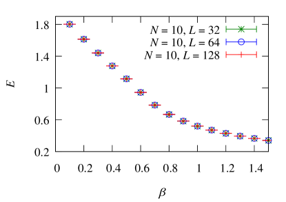
Figure 1: Energy density $E$ as a function of $\beta$ for various $L$’s. The volume dependence is smaller than the dots.

Figure 2: Correlation length squared, $\xi_{G}^{2}$, as a function of $\beta$ for $L=32$ and various $N$’s.

In Fig. 3 we show $\chi_{t}$ as a function of $\beta$ for $L=32$ and $N=2$, $3$, $10$, $21$. We see from Fig. 3 that $\chi_{t}$ is suppressed for larger $\beta$, which qualitatively agrees with exponential suppression in Eq. (19). We would point out that numerically obtained $N\chi_{t}$ has quite nontrivial $N$ dependence, while the convergence of $\xi_{G}^{2}$ at large $N$ is merely monotonic. In fact, as noticed in Fig. 2, $\xi_{G}^{2}$ at $N=10$ is very close to that at $N=21$, from which one may want to conclude that $N=10$ could be already a good approximation for the large-$N$ limit in which analytical formulas are known. In Fig. 3, however, $N\chi_{t}$ at $N=10$ is not such close to the $N=21$ results, and furthermore, around $\beta=0.5$, the $N$ dependence is found to be nonmonotonic. Such prominent differences between $\xi_{G}^{2}$ and $N\chi_{t}$ clearly indicate that numerically obtained $N\chi_{t}$ must have more structures than simple scaling with $\xi_{G}^{2}$. Section V will be devoted to detailed analysis on this question.

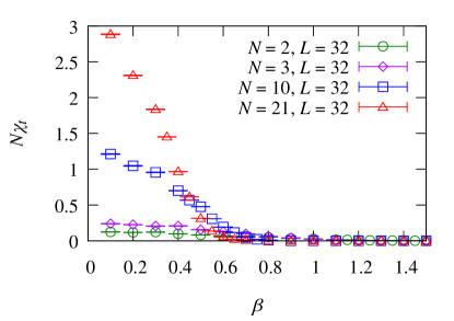
Figure 3: Topological susceptibility, $\chi_{t}$, as a function of $\beta$ for $L=32$ and various $N$’s.

IV Physics Motivation Again

Let us rephrase our physics motivation here in a more concrete way in view of actual data. As we emphasized the ${\mathbb{C}P^{N-1}}$ model is a theoretically clean laboratory to study the topologically winding properties. Because integer $Q$ is a well-defined quantity for any $\beta$, it is a field-theoretically interesting question how the topological properties may change with $\beta$, especially for $\beta$ far from the scaling region. Indeed, as shown in Fig. 3, the topological susceptibility clearly exhibits non-scaling behavior for $\beta\lesssim 0.7$.

Something nontrivial may be happening there, but the information available from $\chi_{t}$ is quite limited. Non-monotonicity may or may not be linked to structural change in instanton-like configurations. In any case there is no way to diagnose what is really happening.

Naively, one could associate $\chi_{t}(\beta)$ with the typical instanton size. For small $\beta$, the correlation length is shorter, and thus the typical instanton size is expected to be smaller too. Then, the system with a fixed volume can accommodate more instantons with smaller size, which enhances the topological susceptibility. If this is the case, it would be naturally anticipated that the topological charge density distribution should contain higher Fourier components for smaller $\beta$. The most straightforward strategy in order to confirm this anticipation is to see the topological charge density profile in Fourier or momentum space. Actually, we will present the Fourier transformed topological charge density in the next section, which will give us a surprise.

We would make a brief comment here for a possible (in principle, but unfeasible at the present) application to QCD physics. We must say that any QCD discussion itself would be beyond the scope of the present paper. Nevertheless, our thinking experiment by means of the ${\mathbb{C}P^{N-1}}$ model has an intriguing analogy to finite-$T$ QCD physics. We are discussing $\beta$-dependence of the topological contents, and it may be sensible to consider $T$-dependence of the topological contents in QCD; actually $\chi_{t}(T)$ has been measured in lattice-QCD simulations, and then the Fourier transformed $\chi_{t}$ may provide us with useful information.

We must not take such an analogy between the ${\mathbb{C}P^{N-1}}$ model and finite-$T$ QCD, however, for the following reason. The parameter $\beta$ in the present study is an inverse temperature for the classical spin model, but the temperature corresponding to finite-$T$ QCD should be introduced in two-dimensional ${\mathbb{C}P^{N-1}}$ model as a (1+1)-dimensional quantum field theory on $S^{1}\times R^{1}$ where the period of $S^{1}$ gives the inverse temperature. Then, $\beta$ would be a coupling constant rather than the inverse temperature, whose scaling property leads to the continuum limit. Eventually, the continuum limit of the ${\mathbb{C}P^{N-1}}$ model is to be mapped into a nonlinear sigma model D’Adda et al. (1978); Witten (1979).

In contrast to this, the present formulation of the ${\mathbb{C}P^{N-1}}$ model represents a classical spin system intrinsically defined on the lattice on $R^{2}$. Such a treatment is quite common for condensed matter physics systems and optical lattice setups Laflamme et al. (2016); Azaria et al. (1995); Beard et al. (2005). In this case the ground state properties, any phase transitions, and excitation spectra are investigated as functions of $\beta$ including values far from the scaling region. There is no imaginary-time direction corresponding to the finite-temperature quantum field theory, but two coordinate axes are both spatial. In this case not only large-$\beta$ regions but entire $\beta$ dependence is considered, and the physical unit is provided by the lattice spacing.

V Image Processing of the Topological Charge Correlator

So far, we have discussed that our simulation results are fully consistent with the previous results. Since the validity has been confirmed, we are now going into more microscopic views of the spatial distribution of the topological charge density. For this image-processing purpose we perform the Fourier analysis, as preannounced in the previous section. As a more convenient measure, we shall introduce the Fourier entropy and demonstrate its usefulness. We also discuss a relation to the SVD analysis which is known as a standard image-processing procedure.

V.1 Fourier Spectral Analysis

In this subsection we present the results from the Fourier spectral analysis at $(N,L)=(10,32)$ only. We shall look further into dependence on $N$ and $L$ when we deal with the entropies in following subsections. We already defined the Fourier transformed topological charge density in Eq. (22). Using this with an ensemble of 1000 configurations, we computed the averaged Fourier power spectrum of the topological charge density, i.e., $\langle|\tilde{\rho}(k)|^{2}\rangle$. We note that $|\tilde{\rho}(k)|^{2}$ is gauge invariant since $\rho(x)$ is already gauge invariant. In other words, $\langle|\tilde{\rho}(k)|^{2}\rangle$ is nothing but a finite-momentum extension of the topological susceptibility, i.e. $\chi_{t}(k^{2})$ as defined in Ref. Shore (1998). Hereafter, we shall use a simple notation of $\chi_{t}(k^{2})$ to mean the Fourier power spectrum. We summarize our results for $\chi_{t}(k^{2})$ computations for $\beta=0.3$, $0.7$, $1.0$ in Fig. 4.

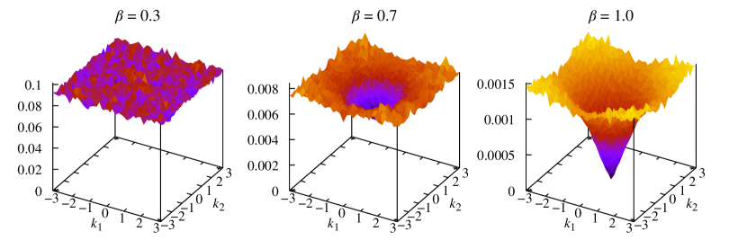
Figure 4: Fourier power spectrum or $\chi_{t}(k^{2})$ for $(N,L)=(10,32)$ and $\beta=0.3$, $0.7$, $1.0$. The momenta $k_{1}$ and $k_{2}$ run from $-\pi$ to $\pi$ in the lattice unit.

We chose these values of $\beta$ according to qualitative changes in the Fourier entropy as we will see later. For $(N,L)=(10,32)$ we will find that $\beta\approx 0.7$ is a “threshold” for suppression of topological excitations, which we denote by $\beta_{\rm th}$.

As long as $\beta\lesssim\beta_{\rm th}$, $\tilde{\rho}(k)$ and thus $\chi_{t}(k^{2})$ spread uniformly over momentum space (see the left panel in Fig. 4). We may say that the topological charge density is “white” then. In contrast to this, small momentum components are significantly suppressed for $\beta\gtrsim\beta_{\rm th}$ and we are inclined to interpret this behavior as suppression of topological excitations. In fact, it is possible that small momentum components of $\chi_{t}(k^{2})$ are more diminished with increasing $\beta$; the spectral intensity at $k=0$ is nothing but $\chi_{t}$, i.e., $\chi_{t}(0)=\langle|\tilde{\rho}(0)|^{2}\rangle=\langle Q^{2}/V\rangle=\chi_{t}$ (where $\langle Q\rangle=0$), and we already observed decreasing $\chi_{t}$ with increasing $\beta$ in Fig. 3.

It is intriguing that the topological charge correlator at finite momenta, $\chi_{t}(k^{2}\neq 0)$, has such a nontrivial shape in momentum space even when $\chi_{t}$ is nearly vanishing. We can give a qualitative explanation for this structure. Although the topological charge itself is robust against perturbative fluctuations, the correlation function has a nonzero contribution from topologically trivial sector. Therefore, we can perform one-loop calculation to find nonzero $\chi_{t}(k^{2})$ for $k$ large enough to justify perturbative treatments as

$$\chi_{t}(k^{2})=\frac{3m_{0}^{2}}{\pi N}+\frac{3k^{2}}{10\pi N}-\frac{k^{2}}{2(2\pi)^{2}\beta N}\,,$$ (28)

where we approximately adopted a continuum theory and we note that the last term with negative sign would be suppressed for large $\beta$ which is assumed in the continuum limit. This quadratic rise of $\chi_{t}(k^{2})$ may partially account for our numerical results at $\beta>\beta_{\rm th}$. At the same time, however, such an interpretation would invalidate our näive anticipation that the system at smaller $\beta$ may accommodate more instantons with smaller size. Therefore, we think that $\chi_{t}(k^{2})$ for large $k$ has inseparable contributions from perturbative fluctuations and small-sized instantons both.

V.2 Fourier Entropy

It would be far more convenient if there is, not a whole profile, but a single observable whose value characterizes changes as in Fig. 4. We propose to use the Fourier entropy defined in Eq. (24) for diagnosis.

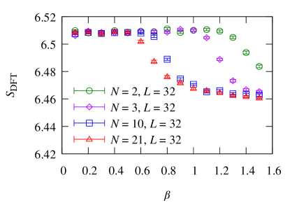
Figure 5: Fourier entropy as a function of $\beta$ for $L=32$ and various $N$.

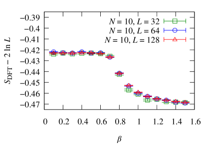
Figure 6: Subtracted Fourier entropy, $S_{\rm DFT}-2\ln L$, as a function of $\beta$ for $N=10$ and various $L$.

Figure 5 shows the Fourier entropy as a function of $\beta$ for $L=32$ and $N=2$, $3$, $10$, $21$. We see that the Fourier entropy stays constant for $\beta\lesssim\beta_{\rm th}$, where $\beta_{\rm th}$ turns out to depend on $N$. Then, the Fourier entropy starts dropping at $\beta_{\rm th}$. As compared to Fig. 4, the threshold behavior is clearly manifested and precisely quantified in Fig. 5.

We also checked the $L$ dependence of the Fourier entropy. We note that the saturated value of $S_{\rm DFT}$ is $2\ln L$ and thus it contains logarithmic $L$ dependence. Interestingly, we found that the subtracted Fourier entropy, $S_{\rm DFT}-2\ln L$, seems to have a well-defined thermodynamic limit. That is, we show the subtracted Fourier entropy as a function of $\beta$ in Fig. 6 for $N=10$ and $L=32$, $64$, $128$. The subtracted Fourier entropy barely has $L$ dependence as confirmed in Fig. 6. This result is consistent with our previous discussion that $L=32$ is already close to the thermodynamic limit.

From these results we could deduce changes in the topological contents as follows. For $\beta\lesssim\beta_{\rm th}$ the topological fluctuations are large as seen in $\chi_{t}$ but the topological contents are white. For $\beta\gtrsim\beta_{\rm th}$ where $S_{\rm DFT}$ starts decreasing, the topological contents with small $k$ are breached, which implies that large-sized domains (possibly instantons) are suppressed simultaneously as the correlation length becomes larger.

V.3 Snapshot Entropy

The Fourier power spectrum is a useful device for the image processing, and a more conventional alternative is the SVD analysis which is suitable for coarse-graining the image. Let us compute the snapshot entropy using the SVD and check whether anything nontrivial appears near $\beta_{\rm th}$ or not.

In Fig. 7 we plot $S_{\rm SVD}$ as a function of $\beta$ for $L=32$ and $N=2$, $3$, $10$, $21$, which is a SVD counterpart of the previous plot in Fig. 5.

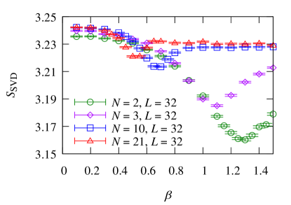
Figure 7: Snapshot entropy, $S_{\rm SVD}$, as a function of $\beta$ for $L=32$ and various $N$.

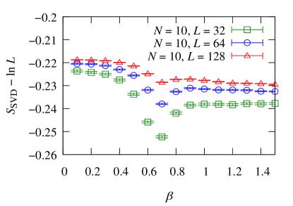
Figure 8: Subtracted snapshot entropy, $S_{\rm SVD}-\ln L$, as a function of $\beta$ for $N=10$ and various $L$.

Instead of clear threshold behavior in Fig. 5, we found that $S_{\rm SVD}$ exhibits a dip around $\beta_{\rm th}$ as seen in Fig. 7. Similarly to the Fourier entropy, in the case of $S_{\rm SVD}$, the depth and the location of the dip depend on $N$. Interestingly, the $L$ dependence of $S_{\rm SVD}$ is quite different from that of $S_{\rm DFT}$. Figure 8 shows the subtracted snapshot entropy, $S_{\rm SVD}-\ln L$, for $N=10$ and $L=32$, $64$, $128$. We see that some sizable $L$ dependence remains even after the subtraction, which makes a sharp contrast to Fig. 6. Such $L$ dependent results are highly nontrivial; we tested $L$-scaling analysis, but the $L$ dependence seen in Fig. 8 turned out not to obey simple scaling. We would point out an example of analytically calculable $S_{\rm SVD}$; in a real random matrix theory, $S_{\rm SVD}^{\rm(RM)}=\ln L-\pi/4$ is known Matsueda (2012). Thus, $L$ dependent $S_{\rm SVD}$ may already indicate that the theory under consideration has some interesting features.

In order to locate $\beta_{\rm th}$ for numerical simulations in a finite size box, $S_{\rm SVD}$ is as useful as $S_{\rm DFT}$. However, it is evident from Fig. 8 that the dip depth becomes shallower for larger $L$, implying that the dip may eventually disappear in the thermodynamic limit unless we know the proper $L$ scaling. Therefore, for a practical usage, $S_{\rm DFT}$ would be a more tractable choice.

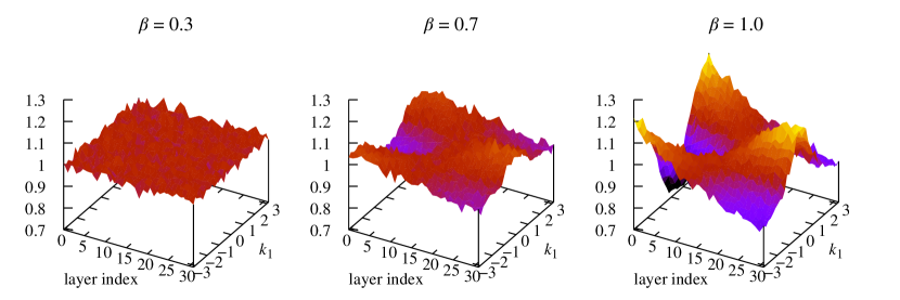
Figure 9: SVD layer dependence of the Fourier spectrum for $(N,L)=(10,32)$ and $\beta=0.3$, $0.7$, $1.0$.

V.4 Correlation between Fourier and Snapshot Entropies

It would be instructive to clarify a possible connection of the Fourier spectrum and the SVD spectrum of the topological charge density. To this end we have calculated the Fourier spectrum of each SVD layer of the topological charge density. We note that each SVD layer is a direct product of two vectors, $U^{(n)}_{x_{1}}V^{(n)}_{x_{2}}$, so that the Fourier transform with respect to two spatial directions is trivially factorized, and we can separately discuss $\tilde{U}^{(n)}(k_{1})$ [that is a Fourier transform of $U^{(n)}_{x_{1}}$] and $\tilde{V}^{(n)}(k_{2})$ [that is a Fourier transform of $V^{(n)}_{x_{2}}$]. From symmetry between 1, 2 directions, clearly, it is sufficient to consider only $\langle|\tilde{U}^{(n)}(k_{1})|^{2}\rangle$ without loss of generality, and Fig. 9 shows our results. We recall that in our convention a smaller SVD layer index corresponds to a larger SVD eigenvalue. We see that the Fourier spectrum is “white” at $\beta\lesssim\beta_{\rm th}$ for all the SVD layers as is the case in the left panel of Fig. 9. Some characteristic patterns start emerging around $\beta_{\rm th}\approx 0.7$ as observed in the middle and the right panels of Fig. 9, namely, images with smaller layer index (i.e., larger SVD eigenvalue) are more dominated by large momentum modes, while images with larger layer index contain smaller momentum modes. Interestingly, this present situation is quite unusual; if the SVD is used for the image processing of ordinary snapshot photographs, usually, smaller SVD index layers would typically correspond to a partial image with smaller momenta or larger spatial domains. A general trend is that such an ordinary correspondence in the image processing holds for classical systems, and for quantum systems the correspondence could be reversed due to quantum fluctuations. It is a subtle question whether $\rho(x)$ belongs to classical or quantum class. Our numerical results suggest a quantum nature, so that if we want to coarse-grain $\rho(x)$, we should remove SVD layers from the smallest index.

The physical interpretation of the Fig. 9 is rather straightforward contrary to the image-processing point of view. As the $\beta$ grows, larger momentum components become relevant in the topological charge density spectrum because of the renormalization scaling of the physical length unit. In the context of the QCD physics, the instantons simply melt away at larger $\beta$ (that is, larger physical temperature). Or, equivalently, larger $\beta$ prohibits topological excitations in larger scale if we regard ${\mathbb{C}P^{N-1}}$ model as the spin model in the condensed matter systems.

VI Discussions from the strong-coupling expansion

We found that the ${\mathbb{C}P^{N-1}}$ model may have transitional behavior as a function of $\beta$, which is not clear in the topological susceptibility $\chi_{t}$ but evidently seen in the Fourier entropy as well as the snapshot entropy. We also clarified that this transitional change is related to the spatial distribution of the topological charge density. Then, an interesting question is what the underlying physics should be.

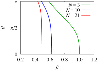
Figure 10: Phase boundary determined from the strong-coupling character expansion up to 10 order. The left (i.e., smaller $\beta$) region from the boundary line indicates the full confinement phase, while the right (i.e., larger $\beta$) region the phase with infinitesimal confinement loss.

A hint comes from the analysis in the large-$N$ limit in which a first-order phase transition occurs with a well-defined $\beta_{\rm c}$. As argued in Ref. Lüscher (1982), the system is completely disordered for $\beta<\beta_{\rm c}$, while the system for $\beta>\beta_{\rm c}$ is still disordered but has a finite correlation length. These changes are qualitatively consistent with our results of Fig. 4.

We can proceed to a further quantitative consideration using the strong-coupling expansion. The pressure or the free energy $F$ is expanded up to order 10 in the character expansion Plefka and Samuel (1997). The physics motivation lies in the phase structure as a function of the coupling $\beta$ and the topological angle $\theta$. We note that a finite $\theta$ causes the sign problem and the lattice numerical simulations would not work reliably then. The string tension between charges $\pm e$ is given by $\sigma(e,\theta,\beta)=F(\theta+2\pi e,\beta)-F(\theta,\beta)$ which is proportional to $\partial F(\theta,\beta)/\partial\theta$ in the limit of $e\to 0$. Then, the extremal condition, $\partial F(\theta,\beta)/\partial\theta=0$, indicates a phase transition associated with loss of confinement of infinitesimal charges. The phase structure inferred from the strong-coupling expansion is illustrated in Ref. Kawauchi and Takeda (2016a) in a way extrapolated to $\theta\simeq 0$ regions for $N=2$. Interestingly, the phase boundary approaches $\beta_{\rm c}=1.2\sim 1.3$ as $\theta\to 0$ (see Fig. 2 of Ref. Kawauchi and Takeda (2016a)). Of course, the strong-coupling analysis may lose validity at such large $\beta$, but the coincidence between this $\beta_{\rm c}=1.2\sim 1.3$ and our $\beta_{\rm th}$ for $N=2$ read from Figs. 5 and 7 is quite suggestive. Taking this quantitative coincidence seriously, as shown in Fig. 10, we drew the phase boundaries for other $N$’s from the condition, $\partial F(\theta,\beta)/\partial\theta=0$, using the expressions in Ref. Plefka and Samuel (1997). Then, those phase boundaries hit $\theta\simeq 0$ at certain values of $\beta$ which are all very close to our $\beta_{\rm th}$.

We would not claim at present that our $\beta_{\rm th}$ can be identified as the critical value of $\beta$ corresponding to the deconfinement phase transition. It is still under investigations whether there is a critical $\beta$ at all; Our present data show no genuine phase transition but only a smooth crossover with transitional behavior. One exotic scenario conjectured in preceding works is that $\beta_{\rm c}\to\infty$ as $\theta\to 0$, and if so, the strong-$CP$ problem may be understood as a requirement for confinement as argued in Refs. Plefka and Samuel (1997); Kawauchi and Takeda (2016a). Our present results do not support $\beta_{\rm c}\to\infty$ but not strictly exclude this scenario. It is still logically possible that, even in such a situation, the phase boundaries may take steeply bending shapes near $\theta\simeq 0$ and transitional remnants may be detectable in the simulation at $\theta=0$ like ours.

However, a more straightforward interpretation would be the following: It is not easy to think of such an abrupt change of $\beta_{\rm c}$ in the small-$\theta$ region. In fact, Fig. 10 implies almost no $\theta$-dependence of $\beta_{\rm c}$ for not large values of $\theta$ (e.g., $\theta\lesssim\pi/4$). For sufficiently (but not too) small $\theta$, we see that $\partial F/\partial\theta\bigr{|}_{\theta}\simeq\partial F/\partial\theta\bigr{|}_{0}+\partial^{2}F/\partial\theta^{2}\bigr{|}_{0}\theta=0$ leads to $\partial^{2}F/\partial\theta^{2}\bigr{|}_{0}\propto\chi_{t}\simeq 0$. Therefore, such a coincidence between $\beta_{\rm c}$ (determined from $\partial F/\partial\theta=0$) and $\beta_{\rm th}$ (where $\chi_{t}\simeq 0$) is not very surprising. Moreover, we can give an intuitive and qualitative argument in favor of $\beta_{\rm c}\simeq\beta_{\rm th}$.

Physically speaking, the confined phase is known to correspond to the disordered state Svetitsky (1986), in which random distributions in Fourier space should be flat as seen in the left of Fig. 4 for $\beta<\beta_{\rm th}$. The point is, as mentioned in Sec. II.3, the Fourier and the snapshot entropies take the maximum values with uncorrelated random distributions. Therefore, if randomness in Fourier space is partially lost as is the case in the middle of Fig. 4 for $\beta\simeq\beta_{\rm th}$, the Fourier entropy starts decreasing. Again, we should remind that it is hard to locate a threshold precisely for such a smooth crossover, and its precise location would depend on the choice of observables and prescriptions.

Indeed, how the crossover looks like is quite different for the snapshot entropy, which starts decreasing around $\beta$ smaller than $\beta_{\rm th}$. This is so, as hinted by Fig. 9, since the SVD layers could have nontrivial structures in Fourier space already when the original configuration as a superposition of the SVD layers does not yet develop significant structures. In this sense, the snapshot entropy is more sensitive to microscopic substructures. However, we would stop such discussions on the snapshot entropy. As we briefly mentioned before, unlike the Fourier entropy, the thermodynamic limit of the snapshot entropy seems to be ill-defined, which itself is quite surprising. There might be interesting underlying mechanism, but it would be out of scope of the current work. For our claim of sudden changes of matter around $\beta_{\rm th}$ and a possible interpretation in terms of infinitesimal deconfinement around $\beta_{\rm c}$, the Fourier entropy, which looks well-defined in the thermodynamic limit, should be sufficient.

For more clarification we need to perform simulations at nonzero $\theta$, but for this purpose, we should circumvent the sign problem of the Monte-Carlo method. Apart from the sign problem, once we could establish that our entropies are sensitive to the phase boundaries, in turn, our entropies should be quite useful probes to quantify $\beta_{\rm c}$ precisely.

VII Conclusions

We conducted the numerical Monte-Carlo simulation using the ${\mathbb{C}P^{N-1}}$ model. We first checked the simulation validity by comparing our results with the precedent studies for $N=2$, $3$, $10$, and $21$. We then scrutinized the spatial distribution of the topological charge density for various inverse temperature $\beta$ by means of the Fourier analysis and the singular value decomposition. There, we found that the Fourier power spectrum of the topological charge density is rather structureless or “white” in momentum space for small $\beta$, while small momentum components become diminished for $\beta$ above a certain threshold $\beta_{\rm th}$, which is possibly interpreted as a suppression of large-sized instantons at large $\beta$. At the same time, nontrivial structures (i.e., a drop in the Fourier entropy and a dip in the snapshot entropy) appear also around $\beta_{\rm th}$. We gave discussions based on the strong-coupling character expansion in an extended $\beta$-$\theta$ plane. Our numerical value of $\beta_{\rm th}$ is suggestively close to critical $\beta_{\rm c}$ of the phase boundary from the strong-coupling expansion at $\theta\to 0$. We gave qualitative arguments in favor of $\beta_{\rm th}\simeq\beta_{\rm c}$ and explained the decreasing behavior of the Fourier entropy accordingly, while the snapshot entropy seems to be ill-defined in the thermodynamic limit and thus its behavior is not under theoretical control in the current analysis.

Nevertheless, we clarified a correlation between the Fourier and the snapshot entropies. In contrast to the ordinary image-processing of picture images, SVD layers with larger SVD eigenvalues turn out to be dominated with higher momentum components. Thus, a cooling method could be implemented by removing the SVD layers from lower index (with larger SVD eigenvalue). A striking finding in this work is that the Fourier power spectrum of the topological charge density or the finite momentum extended topological susceptibility, $\chi_{t}(k^{2})$, has nontrivial momentum dependence even at large $\beta$ when the topological susceptibility itself is nearly vanishing. This indicates that the topological contents of the theory are not necessarily empty even when the topological susceptibility approaches zero if one explores finite momentum regions. One might think that nonzero topological fluctuations at finite momenta may arise purely from perturbative loops and may not necessarily involve topological windings. This is true, and nevertheless, this situation is still interesting. We would recall that such property of $\chi_{t}(k^{2})$ is reminiscent of the sphaleron rate which is a real-time quantity analytically continued from the topological susceptibility. In a seminal work in Ref. Arnold and McLerran (1988) it has been shown that the sphaleron rate has finite contributions from zero winding sector, though the analytical continuation makes such terms disappear in the topological susceptibility. In other words, the sphaleron rate is a finite frequency extension from $\chi_{t}$, and we are discussing a finite spatial momentum extension from $\chi_{t}$, and both are as nontrivial.

One interesting direction would be the lattice calculation of $\chi_{t}(k^{2})$ in the pure Yang-Mills theory at high temperature where $\chi_{t}$ itself is vanishingly small. Then, a nontrivial question is whether the pure Yang-Mills theory and QCD may have the behavior of increasing $\chi_{t}(k^{2})\propto k^{2}$ or not. Alternatively, the measurement of the Fourier entropy using the topological charge density as a function of the physical temperature should be in principle feasible in the pure Yang-Mills theory. Our results imply that the Fourier entropy would show some nonmonotonic behavior near $T_{c}$, which could be tested in the pure Yang-Mills theory in order to quantify how much “white” the topological contents are. It is tricky, however, how to carry out the SVD for three or higher dimensional data, and so the applicability of the snapshot entropy is limited to two-dimensional field theories.

An interesting future problem with special attention to the lattice ${\mathbb{C}P^{N-1}}$ model would be inclusion of interaction terms with farther neighborhood, with which nontrivial phase structures are realized. Another challenging problem in the ${\mathbb{C}P^{N-1}}$ model is how to identify the instantons and the bions numerically in the ${\mathbb{C}P^{N-1}}$ model simulations. In principle, all information on such special configurations should be encoded on the Fourier power spectrum of the topological charge density. Such questions should deserve judicious investigations in the future.