Dandelion++: Lightweight Cryptocurrency Networking with Formal Anonymity Guarantees

Abstract.

Recent work has demonstrated significant anonymity vulnerabilities in Bitcoin’s networking stack. In particular, the current mechanism for broadcasting Bitcoin transactions allows third-party observers to link transactions to the IP addresses that originated them. This lays the groundwork for low-cost, large-scale deanonymization attacks. In this work, we present Dandelion++, a first-principles defense against large-scale deanonymization attacks with near-optimal information-theoretic guarantees. Dandelion++ builds upon a recent proposal called Dandelion that exhibited similar goals. However, in this paper, we highlight some simplifying assumptions made in Dandelion, and show how they can lead to serious deanonymization attacks when violated. In contrast, Dandelion++ defends against stronger adversaries that are allowed to disobey protocol. Dandelion++  is lightweight, scalable, and completely interoperable with the existing Bitcoin network. We evaluate it through experiments on Bitcoin’s mainnet (i.e., the live Bitcoin network) to demonstrate its interoperability and low broadcast latency overhead.

1. Introduction

Anonymity is an important property for a financial system, especially given the often-sensitive nature of transactions (Chellappa and Sin, 2005). Unfortunately, the anonymity protections in Bitcoin and similar cryptocurrencies can be fragile. This is largely because Bitcoin users are identified by cryptographic pseudonyms (a user can have multiple pseudonyms). When a user Alice wishes to transfer funds to another user Bob, she generates a transaction message that includes Alice’s pseudonym, the quantity of funds transferred, the prior transaction from which these funds are drawn, and a reference to Bob’s pseudonym (Nakamoto, 2008). The system-wide sequence of transactions is recorded in a public, append-only ledger known as the blockchain. The public blockchain means that users only remain anonymous as long as their pseudonyms cannot be linked to their true identities.

This mandate has proved challenging to uphold in practice. Several vulnerabilities have enabled researchers, law enforcement, and possibly others to partially deanonymize users (Bohannon, 2016). Publicized attacks have so far included: (1) linking different public keys that belong to the same user (Meiklejohn et al., 2013), (2) associating users’ public keys with their IP addresses (Biryukov et al., 2014; Koshy et al., 2014), and in some cases, (3) linking public keys to human identities (Frizell, 2015). Such deanonymization exploits tend to be cheap, easy, and scalable (Meiklejohn et al., 2013; Biryukov et al., 2014; Koshy et al., 2014).

Although researchers have traditionally focused on the privacy implications of the blockchain (Ober et al., 2013; Ron and Shamir, 2013; Meiklejohn et al., 2013), we are interested in lower-layer vulnerabilities that emerge from Bitcoin’s peer-to-peer (P2P) network. Recent work has demonstrated P2P-layer anonymity vulnerabilities that allow transactions to to be linked to users’ IP addresses with accuracies over 30% (Biryukov et al., 2014; Koshy et al., 2014). Understanding how to patch these vulnerabilities without harming utility remains an open question. The goal of our work is to propose a practical, lightweight modification to Bitcoin’s networking stack that provides theoretical anonymity guarantees against the types of attacks demonstrated in (Biryukov et al., 2014; Koshy et al., 2014), and others. We begin with an overview of Bitcoin’s P2P network, and explain why it enables deanonymization attacks.

Bitcoin’s P2P Network. Bitcoin nodes are connected over a P2P network of TCP links. This network is used to communicate transactions, the blockchain, and control packets, and it plays a crucial role in maintaining the network’s consistency. Each peer is identified by its (IP address, port) combination. Whenever a node generates a transaction, it broadcasts a record of the transaction over the P2P network; critically, transaction messages do not include the sender’s IP address—only their pseudonym. Since the network is not fully-connected, transactions are relayed according to epidemic flooding (Peterson and Davie, 2007). This ensures that all nodes receive the transaction and can add it to the blockchain. Hence, transaction broadcasting enables the network to learn about them quickly and reliably.

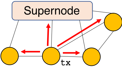
Figure 1. Supernodes can observe relayed transaction propagation metadata to infer which node was the source of a transaction message (tx).

However, the broadcasting of transactions can also have negative anonymity repercussions. Bitcoin’s current broadcast mechanism spreads content isotropically over the graph; this allows adversarial peers who observe the spreading dynamics of a given transaction to infer the source IP of each transaction. For example, in recent attacks (Biryukov et al., 2014; Koshy et al., 2014), researchers launched a supernode (disguised as a regular node) that connected to all P2P nodes (Figure 1) and logged their relayed traffic. This allowed the supernode to observe the spread of each transaction over the network over time, and ultimately infer the source IP. Since transaction messages include the sender’s pseudonym, the supernodes were able to deanonymize users, or link their pseudonyms to an IP address (Biryukov et al., 2014; Koshy et al., 2014). Such deanonymization attacks are problematic because of Bitcoin’s transparency: once a user is deanonymized, her other transactions can often be linked, even if she creates fresh pseudonyms for each transaction (Meiklejohn et al., 2013).

There have been recent proposals for mitigating these vulnerabilities, included broadcasting protocols that reduce the symmetry of epidemic flooding. Bitcoin Core (bit, 2015), the most popular Bitcoin implementation, adopted a protocol called diffusion, where each node spreads transactions with independent, exponential delays to its neighbors on the P2P graph. Diffusion is still in use today. However, proposed solutions (including diffusion) tend to be heuristic, and recent work shows that they do not provide sufficient anonymity protection (Fanti and Viswanath, 2017). Other proposed solutions, such as Dandelion (Bojja Venkatakrishnan et al., 2017), offer theoretical anonymity guarantees, but do so under idealistic assumptions that are unlikely to hold in practice. The aim of this work is to propose a broadcasting mechanism that (a) provides provable anonymity guarantees under realistic adversarial and network assumptions, and (b) does not harm the network’s broadcasting robustness or latency. We do this by revisiting the Dandelion system and redesigning it to withstand a variety of practical threats.

Contributions. The main contributions of this paper are threefold:

(1) We identify key idealistic assumptions made by Dandelion (Bojja Venkatakrishnan et al., 2017), and show how anonymity is degraded when those assumptions are violated. In particular, (Bojja Venkatakrishnan et al., 2017) assumes an honest-but-curious adversary that has limited knowledge of the P2P graph topology and only observes one transaction per node. If adversaries are instead malicious and collect more information over time, we show that they are able to weaken the anonymity guarantees of (Bojja Venkatakrishnan et al., 2017) through a combination of attacks, including side information, graph manipulation, black hole, and intersection attacks.

(2) We propose a modified protocol called Dandelion++  that subtly changes most of the implementation choices of Dandelion, from the graph topology to the randomization mechanisms for message forwarding. Mathematically, these (relatively small) algorithmic changes completely change the anonymity analysis by exponentially augmenting the problem state space. Using analytical tools from Galton-Watson trees and random processes over graphs, we evaluate the anonymity tradeoffs of Dandelion++, both theoretically and in simulation, against stronger adversaries. The main algorithmic changes in Dandelion++ rely on increasing the amount of information the adversary must learn to deanonymize users. Technically, the anonymity proofs require us to bound the amount of information a single node can pass to the adversary; on a line graph, this is easy to quantify, but on more complicated expander graphs, this requires reasoning about the random routing decisions of each node in a local neighborhood. Exploiting the locally-tree-like properties of such graphs allows us to analyze these settings with tools from the branching process literature.

(3) We demonstrate the practical feasibility of Dandelion++  by evaluating an implementation on Bitcoin’s mainnet (i.e., the live Bitcoin network). We show that Dandelion++ does not increase latency significantly compared to current methods for broadcasting transactions, and it is robust to node failures and misbehavior.

The paper is structured as follows: in §2, we discuss relevant work on anonymity in cryptocurrencies and P2P networks. In §3, we present our adversarial model, which is based on prior attacks in the literature. §2 presents Dandelion  in more detail; in §4, we analyze Dandelion’s weaknesses, and propose Dandelion++  as an alternative. We present experimental evaluation results in §5, and discuss the implications of these results in §6.

2. Related Work

The anonymity properties of cryptocurrencies have been studied extensively. Several papers have exploited anonymity vulnerabilities in the blockchain (Androulaki et al., 2013; Reid and Harrigan, 2013; Ober et al., 2013; Ron and Shamir, 2013; Meiklejohn et al., 2013), suggesting that transactions by the same user can be linked, even if the user adopts different addresses (Meiklejohn et al., 2013). In response, researchers proposed alternative cryptocurrencies and/or tumblers that provide anonymity at the blockchain level (Maxwell, 2013; mon, [n. d.]; Sasson et al., 2014; Ruffing et al., 2014; Heilman et al., 2016; Jedusor, 2016). In 2014, researchers turned to the P2P network, showing that regardless of blockchain implementation, users can be deanonymized by network attackers (Koshy et al., 2014; Biryukov et al., 2014; Biryukov and Pustogarov, 2015; Fanti and Viswanath, 2017). Researchers were able to link transactions to IP addresses with accuracies over 30% (Biryukov et al., 2014). These attacks proceeded by connecting a supernode to most all active Bitcoin server nodes. More recently, (Apostolaki et al., 2016) demonstrated the serious anonymity and routing risks posed by an AS-level attacker. These papers suggest a need for networking protocols that defend against deanonymization attacks.

Anonymous communication for P2P/overlay networks has been an active research topic for decades. Most work relies on two ideas: randomized routing (e.g., onion routing, Chaumian mixes) and/or dining cryptographer (DC) networks. Systems that use DC nets (Chaum, 1988) are typically designed for broadcast communication, which is our application of interest. However, DC nets are known to be inefficient and brittle (Golle and Juels, 2004). Proposed systems (Goel et al., 2003; Zamani et al., 2013; Corrigan-Gibbs and Ford, 2010; Wolinsky et al., 2012) have improved these properties significantly, but DC networks never became scalable enough to enjoy widespread adoption in practice.

Systems based on randomized routing are generally more efficient, but focus on point-to-point communication (though these tools can be adapted for broadcast communication). Early works like Crowds (Reiter and Rubin, 1998), Tarzan (Freedman and Morris, 2002), and P5 (Sherwood et al., 2005) paved the way for later practical systems, such as Tor (Dingledine et al., 2004) and I2P (Zantout and Haraty, 2011), as well as recent proposals like Drac (Danezis et al., 2010), Pisces (Mittal et al., 2013), and Vuvuzela (van den Hooff et al., [n. d.]). Our work differs from this body of work along two principal axes: (1) usage goals, and (2) analysis metrics/results.

(1) Usage goals. Among tools with real-world adoption, Tor (Dingledine et al., 2004) is the most prominent; privacy-conscious Bitcoin users frequently use it to anonymize transmissions. However, expecting Bitcoin users to route their traffic through Tor (or a similar service) poses several challenges, depending on the mode of integration. One option would be to hard-code Tor-like functionality into the cryptocurrency’s networking stack; for instance, Monero is currently integrating onion routing into its network (kov, [n. d.]). However, this requires significant engineering effort; Monero’s development effort is still incomplete after four years (red, 2016), and no other major cryptocurrencies (Bitcoin, Ethereum, Ripple) have announced plans to integrate anonymized routing. Principal challenges include the difficulty of implementing cryptographic protocols correctly, as well as the fact that onion routing clients need global, current network information to determine transaction paths, whereas existing systems (and Dandelion++) make local connectivity and routing decisions. Another option would be to have users route their transactions through Tor. However, many Bitcoin users are unaware of Bitcoin’s privacy vulnerabilities and/or may lack the technical expertise to route their transactions through Tor. Our goal in Dandelion++is instead to propose simple, lightweight solutions that can easily be implemented within existing cryptocurrencies, with privacy benefits for all users.

(2) Analysis. The differences in analysis are more subtle. Many of the above systems include theoretical analysis, but none provide optimality guarantees under the metrics discussed in this paper. Prior work in this space has mainly analyzed per-user metrics, such as probability of linkage (Reiter and Rubin, 1998; Freedman and Morris, 2002; van den Hooff et al., [n. d.]). For example, Crowds provides basic linkability analysis (Reiter and Rubin, 1998), and Danezis et al. show that Crowds has an optimally-low probability of detection under a simple first-spy estimator that assigns each transaction to the first honest node to deliver the transaction to the adversary (Danezis et al., 2009). Such analysis overlooks the fact that adversaries can use more sophisticated estimators based on data from many users to execute joint deanonymization. We consider the (more complex) problem of population-level joint deanonymization over realistic graph topologies, using more nuanced estimators and anonymity metrics. Indeed under the metrics we study, Crowds is provably sub-optimal (Bojja Venkatakrishnan et al., 2017). We maintain that joint deanonymization is a realistic adversarial model as companies are being built on the premise of providing network-wide identity analytics (e.g. Chainalysis (cha, [n. d.])). In addition to using a different anonymity metric, the protocols of prior work exhibit subtle differences that significantly change the corresponding anonymity analyses and guarantees. We will highlight these differences when the protocols and analysis are introduced.

The most relevant solution to our problem is a recent proposal called Dandelion (Bojja Venkatakrishnan et al., 2017), which uses statistical obfuscation to provide anonymity against distributed, resource-limited adversaries (pseudocode in Appendix A). Dandelion propagates transactions in two phases: (i) an anonymity (or stem) phase, and (ii) a spreading (or fluff) phase. In the anonymity phase, each message is passed to a single, randomly-chosen neighbor in an anonymity graph $H$ (this graph can be an overlay of the P2P graph $G$). This propagation continues for a geometric number of hops with parameter $q$. However, unlike related prior work (e.g., Crowds (Reiter and Rubin, 1998)), different users forward their transactions along the same path in the anonymity graph $H$, which is chosen as a directed cycle in (Bojja Venkatakrishnan et al., 2017); this small difference causes Crowds to be sub-optimal under the metrics studied here and in (Bojja Venkatakrishnan et al., 2017), and significantly affects the resulting anonymity guarantees. In the spreading phase, messages are flooded over the P2P network $G$ via diffusion, just as in today’s Bitcoin network. Dandelion periodically re-randomizes the line graph, so the adversaries’ knowledge of the graph is assumed to be limited to their immediate neighborhood.

Under restrictive adversarial assumptions, Dandelion  exhibits near-optimal anonymity guarantees under a joint-deanonymization model (Bojja Venkatakrishnan et al., 2017). Our work illustrates Dandelion’s fragility to basic Byzantine attacks and proposes a scheme that is robust to Byzantine intersection attacks. This relaxation requires completely new analysis, which is the theoretical contribution of this paper.

3. Model

3.1. Adversary

The adversaries studied in prior work exhibit two basic capabilities: creating nodes and creating outbound connections to other nodes. At one extreme, a single supernode can establish outbound connections to every node in the network; this resembles recent attacks on the Bitcoin P2P network (Biryukov et al., 2014; Koshy et al., 2014) and related measurement tools (Koshy, 2013; Miller et al., 2015). At the other extreme is a botnet with many honest-but-curious nodes, each of which creates few outbound edges according to protocol. This captures the adversarial model in (Bojja Venkatakrishnan et al., 2017) and botnets observed in Bitcoin’s P2P network (McMillen, 2017). In this paper, we combine both models: a botnet adversary that can corrupt some fraction of Bitcoin nodes and establish arbitrarily many outbound connections.

We model the botnet adversary as a set of colluding hosts spread over the network. Out of $n$ total peers in the network, we assume a fraction $p$ (i.e., $np$ peers) are malicious. The botnet seeks to link transactions and their associated public keys with the IP addresses of the hosts generating those transactions. The adversarial hosts (or spies) need not follow protocol. Spies can generate as many outbound edges as they want, to whichever nodes they choose; however, they cannot force honest nodes to create outbound edges to spies. The spies perform IP address deanonymization by observing the transaction propagation patterns in the network. Adversaries log transaction information, including timestamps, sending hosts, and control packets. This information, along with global knowledge (e.g., network structure) is used to deanonymize honest users.

We assume adversaries are interested in mass deanonymization, and our anonymity metrics (Section 3.2) capture the adversary’s success at both the individual level and the population level. This differs from a setting where the adversary seeks to deanonymize a targeted user. While the latter is a more well-studied problem (Bohannon, 2016; Biryukov and Pustogarov, 2015; Androulaki et al., 2013), our adversarial model is motivated in part by the growing market for wide-area cryptocurrency analytics (e.g., Chainalysis (cha, [n. d.])). Our goal is to provide network-wide anonymity that does not require users to change their behavior. While this approach will not stop targeted attacks, it does provide a first line of defense against broad deanonymization attacks that are currently feasible.

Note that recent work on ISP- or AS-level adversaries (Apostolaki et al., 2016) can be modeled as a special case of this botnet adversary, except edges rather than nodes are corrupted. This adversary is outside the scope of this paper, but the topic is of great interest. A principal challenge with ISP-level adversaries is that they can eclipse nodes; under such conditions, routing-based defenses (like Dandelion++) cannot provide any guarantees for a targeted node. Nonetheless, in §6, we discuss the compatibility of our proposed methods with the countermeasures proposed in (Apostolaki et al., 2016) for large-scale adversaries.

3.2. Anonymity Metrics: Precision and Recall

The literature on anonymous communication has proposed several metrics for studying anonymity. The most common of these captures an adversary’s ability to link a single transaction to a single user’s IP address; this probability of detection, and variants thereof, have been the basis of much anonymity analysis (Chaum, 1988; Reiter and Rubin, 1998; Danezis et al., 2009; Fanti et al., 2015; van den Hooff et al., [n. d.]). However, this class of metrics does not account for the fact that adversaries can achieve better deanonymization by observing other users’ transactions. We consider such a form of joint decoding.

The adversary’s goal is to associate transactions with users’ IP addresses through some association map. This association map can be interpreted as a classifier that classifies each transaction (and its corresponding metadata) to an IP address. Hence an adversary’s deanonymization capabilities can be measured by evaluating the adversary’s associated classifier. We adopt a common metric for classifiers: precision and recall. As discussed in (Bojja Venkatakrishnan et al., 2017), precision and recall are a superset of the metrics typically studied in this space; in particular, recall is equivalent (in expectation) to probability of detection. On the other hand, precision can be interpreted as a measure of a node’s plausible deniability; the more transactions get mapped to a single node, the lower the adversary’s precision.

Let $V_{H}$ denote the set of all IP addresses of honest peers in the network, and let $\tilde{n}=|V_{H}|$ denote the number of honest peers. In this work, a transaction is abstracted as a tuple containing the sender’s address, the recipient’s address, and a payload. To begin, we will assume that each peer $v\in V_{H}$ generates exactly one transaction $X_{v}$. We relax this assumption in §4.2. Let $\mathcal{X}=\cup_{v\in V_{H}}X_{v}$ denote the set of all transactions. We assume the sets $V_{H}$ and $\mathcal{X}$ are known to the adversaries. Let $\mathtt{M}:\mathcal{X}\rightarrow V_{H}$ denote the adversary’s map from transaction $x\in\mathcal{X}$ to IP address $\mathtt{M}(x)\in V_{H}$. The precision and recall of $\mathtt{M}$ at any honest peer $v\in V_{H}$ are given, respectively, by

(1) $$D(v) =\frac{\mathds{1}(\mathtt{M}(X_{v})=v)}{\sum_{u\in V_{H}}\mathds{1}(\mathtt{M}(X_{u})=v)}$$

(2) $$R(v) =\mathds{1}(\mathtt{M}(X_{v})=v),$$

where $\mathds{1}(\cdot)$ denotes the indicator function. Precision (denoted $D(v)$) measures accuracy by normalizing against the number of transactions associated with $v$. A large number of transactions mapped to $v$ implies a greater plausible deniability for $v$. Recall (denoted $R(v)$) measures the accuracy or completeness of the mapping. We define the average precision and recall for the network as $D=\frac{\sum_{v\in V_{H}}D(v)}{|V_{H}|}$ and $R=\frac{\sum_{v\in V_{H}}R(v)}{|V_{H}|}$. In our theoretical analyses under a probabilistic model (see §3.3), we will be interested in the expected values of these quantities, denoted by $\mathbf{D}$ and $\mathbf{R}$, respectively.

Fundamental bounds. (Bojja Venkatakrishnan et al., 2017) shows fundamental lower bounds on the expected precision and recall of any spreading mechanism. In particular, no spreading algorithm can achieve lower expected recall than $p$, where $p$ is the fraction of spy nodes, or expected precision lower than $p^{2}$. These lower bounds assume an honest-but-curious adversary, in which case the recall lower bound is tight, and the precision bound is within a logarithmic factor of tight. However, the solution in (Bojja Venkatakrishnan et al., 2017) does not consider Byzantine adversaries. Hence in this work, we will aim to match these fundamental lower bounds for an honest-but-curious adversary, while also providing robustness against a Byzantine adversary. Obtaining tight lower bounds for general Byzantine adversaries remains an open question, though the lower bounds from (Bojja Venkatakrishnan et al., 2017) naturally still hold. We will show in Section 4.2 that for certain classes of Byzantine adversaries, we can achieve (Bojja Venkatakrishnan et al., 2017)’s lower bound on expected recall and within a logarithmic factor of its lower bound on precision.

3.3. Transaction and Network Model

We follow the probabilistic network model of (Bojja Venkatakrishnan et al., 2017, §2). We assume a uniform prior on $X_{v}$ over the set $\mathcal{X}$, i.e., the ordered tuple $(X_{v_{1}},X_{v_{2}},\ldots,X_{v_{\tilde{n}}})$ is a uniform random permutation of messages in $\mathcal{X}$ where $V_{H}=\{v_{1},v_{2},\ldots,v_{\tilde{n}}\}$. We also assume transaction times are unknown to the adversary.

Input: Set $V=\{v_{1},v_{2},\ldots,v_{n}\}$ of nodes;

Output: A connected, directed graph $G(V,E)$ with average degree $2\eta$

for $v\leftarrow V$ do

       /* pick $\eta$ random targets */

       $N\leftarrow\emptyset$

       for $i\leftarrow\{1,\ldots,\eta\}$ do

             $e\sim$ Unif$(V\setminus\{v\}\setminus N)$

             $N\leftarrow N\cup\{e\}$

       end for

      /* make connections */

       $E=E\cup\{(v\rightarrow u),~{}u\in N\}$

end for

return $G(V,E)$

Algorithm 1 Approximate $2\eta$-Regular Graph

We model the Bitcoin network as a directed graph $G(V,E)$ where the vertices $V=V_{H}\cup V_{A}$ comprise honest peers $V_{H}$ and adversarial peers $V_{A}$. The edges $E$ correspond to TCP links between peers in the network. Although these links are technically bidirectional, the Bitcoin network treats them as directed. An outbound link from Alice to Bob is one that Alice initiated (and vice versa for inbound links); we also refer to the tail node of an edge as the one that originated the connection.

To construct the Bitcoin network, each node establishes up to eight outbound connections, and maintains up to 125 total connections (bit, [n. d.]). In practice, the eight outbound connections are chosen from each node’s locally-maintained address book; we assume each node chooses outbound connections randomly from the set of all nodes (Algorithm 1). This graph construction model results in a random graph where each node has expected degree $2\eta=16$. Although this approximates the behavior of many nodes in Bitcoin’s P2P network, Byzantine nodes need not follow protocol. We will describe the behavior of Byzantine nodes as needed in the paper.

Upon creating a transaction message, peers propagate it according to a pre-specified spreading policy. The propagation dynamics are observed by the spies, whose goal is to estimate the IP addresses of transaction sources. For each transaction $x\in\mathcal{X}$ received by adversarial node $a\in V_{A}$, the tuple $(x,v,t)$ is logged where $v$ is the peer that sent the message to $a$, and $t$ is the timestamp when the message was received. The botnet adversary may also know partial information about the network structure. Clearly, peers neighboring adversarial nodes are known. However in some cases the adversary might also be able to learn the locations of honest peers not directly connected to botnet nodes, either through adversarial probing or side information. For simplicity, we use $\mathbf{O}$ to denote all observed information—message timestamps, knowledge of the graph, and any other control packets—known to the adversary. Given these observations, one common source estimator is the simple-yet-robust first-spy estimator, used in (Biryukov et al., 2014; Koshy et al., 2014; Danezis et al., 2009). Recall that the first-spy estimator outputs the first honest node to deliver a given transaction to the adversary as the source.

Table 1. Summary of changes proposed in Dandelion++, with references to relevant evidence and/or analysis.

Attack	Effect on Dandelion (Bojja Venkatakrishnan et al., 2017)	Dandelion++
		Proposed solution	Effect
Graph-learning (§4.1)	Order-level precision increase (Bojja Venkatakrishnan et al., 2017)	4-regular anonymity graph	Limits precision gain (Thm. 1, Fig. 3)
Intersection (§4.5)	Empirical precision increase (Fig. 6)	Pseudorandom forwarding	Improved robustness (Thm. 2)
Graph-construction (§4.3)	Empirical precision increase (Fig. 9)	Non-interactive construction	Reduces precision gain (Figs. 9, 9)
Black-hole (§4.4)	Transactions do not propagate	Random stem timers	Provides robustness (Prop. 3)
Partial deployment (§4.5)	Arbitrary recall increase (Fig. 12)	Blind stem selection	Improves recall (Thm. 3, Fig. 12)

4. Dandelion++

Dandelion’s theoretical anonymity guarantees make three idealized assumptions: (1) all nodes obey the protocol, (2) each node generates exactly one transaction, (3) all Bitcoin nodes run Dandelion. None of these assumptions necessarily holds in practice. In this section, we show how Dandelion’s anonymity properties break when the assumptions are violated, and propose a modified solution called Dandelion++  that addresses these concerns. Dandelion++ passes transactions over intertwined paths, or ‘cables’, before diffusing to the network (Fig. 2). In practice, these cables may be fragmented (i.e. all nodes are not connected in a single Hamiltonian cycle), but the cable intuition applies within each node’s local neighborhood.

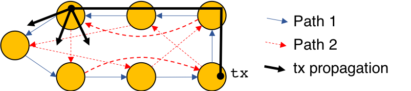
Figure 2. Dandelion++  forwards messages over one of two intertwined paths on a 4-regular graph, then broadcasts using diffusion. Here, tx propagates over the blue solid path.

We begin with a brief description of Dandelion++, and then give a more nuanced picture of how this design came about. We start with Dandelion as a baseline, adopting the same ‘stem phase’ and ‘fluff phase’ terminology, along with dandelion spreading (Algorithm 4). Like Dandelion, Dandelion++ proceeds in asynchronous epochs; each node advances its epoch when its internal clock reaches some threshold (in practice, this will be on the order of 10 minutes). Within an epoch, the main algorithmic components of Dandelion++ are:
(1) Anonymity Graph: Use a random, approximately-4-regular graph instead of a line graph for the anonymity phase (§4.1). This quasi-4-regular graph is embedded in the underlying P2P graph by having each node choose (up to) two of its outbound edges, without replacement, uniformly at random as Dandelion++ relays (§4.3). The choice of Dandelion++ relays should be independent of whether the outbound neighbors support Dandelion++ or not (§4.5). Each time a node changes epoch, it selects fresh Dandelion++ relays.
(2) Transaction Forwarding (own): Every time a node generates a transaction of its own, it forwards the transaction, in stem phase, along the same outbound edge in the anonymity graph. In Dandelion, nodes are assumed to generate only one transaction, so this behavior is not considered in prior analysis.
(3) Transaction Forwarding (relay): Each time a node receives a stem-phase transaction from another node, it either relays the transaction or diffuses it. The choice to diffuse transactions is pseudorandom, and is computed from a hash of the node’s own identity and epoch number. Note that the decision to diffuse does not depend on the transaction itself—in each epoch, a node is either a diffuser or a relay node for all relayed transactions. If the node is not a diffuser in this epoch (i.e., it is a relayer), then it relays transactions pseudorandomly; each node maps each of its incoming edges in the anonymity graph to an outbound edge in the anonymity graph (with replacement). This mapping is selected at the beginning of each epoch, and determines how transactions are relayed (§4.2).
(4) Fail-Safe Mechanism: Each node tracks, for each stem-phase transaction that was sent or relayed, whether the transaction is seen again as a fluff-phase transaction within some random amount of time. If not, the node starts to diffuse the transaction (§4.4).

These small algorithmic changes completely alter the anonymity analysis by introducing an exponentially-growing state space. For example, moving from a line graph to a 4-regular graph (item (1)) invalidates the exact probability computation in (Bojja Venkatakrishnan et al., 2017), and requires a more complex analysis to understand effects like intersection attacks. We also simulate the proposed mechanisms for all attacks and find improved anonymity compared to Dandelion.

The remainder of this section is structured according to Table 1. The weak adversarial model in (Bojja Venkatakrishnan et al., 2017) enables five distinct attacks: graph learning attacks, intersection attacks, graph construction attacks, black hole attacks, and deployment attacks. For each attack, we first demonstrate its impact on anonymity (and/or robustness); in many cases, these effects can lead to arbitrarily high deanonymization accuracies. Next, we propose lightweight implementation changes to mitigate this threat, and justify these choices with theoretical analysis and simulations.

4.1. Graph-Learning Attacks

Theoretical results in (Bojja Venkatakrishnan et al., 2017) assume that the anonymity graph is unknown to the adversary; that is, the adversary knows the randomized graph construction protocol, but it does not know the realization of that protocol outside its own local neighborhood. Under these conditions, Dandelion, which uses a line topology, achieves a maximum expected precision of $O(p^{2}\log(1/p))$, which is near-optimal (recall that $p$ denotes the fraction of malicious nodes in the network). However, if an adversary somehow learns the anonymity graph, the maximum expected precision increases to $O(p)$ (Bojja Venkatakrishnan et al., 2017, Proposition 4)—an order-level increase. On the other hand, recall guarantees do not change if the adversary learns the graph. This is because under dandelion spreading (Algorithm 4), the first-spy estimator is recall-optimal (Bojja Venkatakrishnan et al., 2017), meaning it maximizes the adversary’s expected recall. Since the first-spy estimator is graph-independent, learning the graph does not improve the adversary’s maximum expected recall. A natural question is whether one can avoid this jump in precision.

Dandelion proposes a heuristic solution in which the line graph is periodically reshuffled to a different (random) line graph (Bojja Venkatakrishnan et al., 2017). The intuition is that changing the line graph frequently does not allow enough time for the adversaries to learn the graph. However, the efficacy of this heuristic is difficult to evaluate. Fundamentally, the problem is that it is unclear how fast an adversary can learn a graph, which calls into question the resulting anonymity guarantees.

4.1.1. Proposal: 4-Regular Graphs

We explore an alternative solution that may protect against adversaries that are able to learn the anonymity graph—either due to the Dandelion++ protocol itself or other implementation issues. In particular, we suggest that Dandelion++  should use random, directed, 4-regular graphs instead of line graphs as the anonymity graph topology. 4-regular graphs naturally extend line graphs, which are 2-regular. For now, we study exact 4-regular graphs, though the final proposal uses approximate 4-regular graphs. Although the forwarding mechanism is revisited in §4.2, for now, let us assume that users relay transactions randomly to one of their 2 outbound neighbors in the 4-regular graph until fluff phase.

Although theoretical analysis of expected precision on $d$-regular anonymity graphs is challenging for $d>2$, we instead simulate randomized spreading over different topologies, while measuring anonymity empirically using theoretically-optimal (or near-optimal) estimators. Figure 3 plots the average precision obtained on $d$-regular graphs, for $d=2$ (corresponding to a line graph), 4 and 6, as a function of $p$, the fraction of adversaries, for a network of 50 nodes. Since we are (for now) studying exact 4-regular graphs, the adversarial nodes also have degree 4; this assumption will be relaxed in later sections. The blue solid line at the bottom corresponds to the line graph when the graph is unknown to the adversary; this matches the theoretical precision of $O(p^{2}\log(1/p))$ shown in (Bojja Venkatakrishnan et al., 2017). The solid lines in Figure 3 (i.e., unknown graph) were generated by running the first-spy estimator, which maps each transaction to the first honest node that forwarded the transaction to an adversarial node. When the graph is unknown, we show in Theorem 1 that the first-spy estimator is within a constant factor of optimal; hence, Figure 3 shows results from an approximately-precision-optimal estimator.

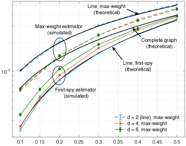
Figure 3. Average precision as a function of $p$ for random, directed $d$-regular graphs.

When the graph is known, we approximate the maximum-precision estimator differently. (Bojja Venkatakrishnan et al., 2017) showed that the precision-optimal estimator is a maximum-weight matching from transactions to nodes, where the weight of the edge between node $v$ and transaction $x$ is the posterior probability $\mathbb{P}(X_{v}=x|\mathbf{O})$ (Theorem 3, (Bojja Venkatakrishnan et al., 2017)). Since the anonymity graph contains cycles, this posterior is difficult to compute exactly, because it requires (NP-hard) enumeration of every path between a candidate source and the first spy to observe a given transaction (Schrijver, 2002). We therefore approximate the posterior probabilities by assuming that each candidate source can only pass a given message along the shortest path to the spy that first observes the message (note that the shortest path is also the most likely one). This path likelihood can be computed exactly and used as a proxy for the desired posterior probability. Given these approximate likelihoods, we compute a maximum-weight matching, and calculate the precision of the resulting matching.

Assuming the adversary knows the graph and uses this quasi-precision-optimal estimator, the precision on a line graph increases to the blue dotted line at the top of the plot. For example, at $p=0.15$, knowing the graph gives a precision boost of 0.12, or about $250$% over not knowing the graph. On the other hand, if a 4-regular graph is unknown to the adversary, it has a precision very close to that of line graphs (orange solid line in Figure 3). But if the graph becomes known to the adversary (orange dotted line), the increase in precision is smaller. At $p=0.15$, the gain is $0.06$—half as large as the gain for line graphs. This suggests that 4-regular graphs are more robust than lines to adversaries learning the graph, while sacrificing minimal precision when the adversary does not know the graph.

Figure 3 also highlights a distinct trend in precision values, as the degree $d$ varies. If the adversary has not learned the topology, then line graphs have the lowest expected precision and hence offer the best anonymity. As the degree $d$ increases, the expected precision progressively worsens until $d=n$, where $n$ is the number of peers in the network. When $d=n$ (i.e., the graph is a complete graph), peers forward their transactions to a random peer in each hop of the dandelion stem. On the other hand, if the topologies are known to the adversary, then the performance trend reverses. In this case, line graphs (for $d=2$) have the worst (highest) expected precision among random $d$-regular graphs; As the degree increases, precision decreases monotonically until $d=n$.

Finally, recall that our simulations used the ‘first-spy’ estimator as the deanonymization policy for $d$-regular graphs when the graph is unknown to the adversary. A priori, it is not clear whether this is an optimal estimator for $d$-regular graphs for $d\geq 4$ ((Bojja Venkatakrishnan et al., 2017) shows that the first-spy estimator is optimal for line graphs). As such the optimal precision curve could be much higher than the one plotted in Figure 3. However, the following theorem—our first main theoretical contribution of this paper—shows that this is not the case.

Theorem 1.

The maximum expected precision on a random 4-regular graph with graph unknown to the adversary is bounded by $\mathbf{D}_{\mathtt{OPT}}\leq 8\mathbf{D}_{\mathtt{FS}}+6p^{2}+O(p^{3}),$ where $\mathbf{D}_{\mathtt{OPT}}$ and $\mathbf{D}_{\mathtt{FS}}$ denote the expected precision under the optimal and first-spy estimators respectively.

(Proof in Appendix B.1) The proof of this result relies on bounding the amount of information that a single node can pass to the adversary, and enumerating the local graph topologies that a single node can see.

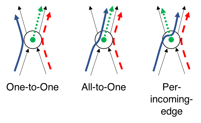
Figure 4. Pseudorandom forwarding. Thick, colored lines denote forwarding rules for incoming edges and the node’s own transactions (green dotted line).

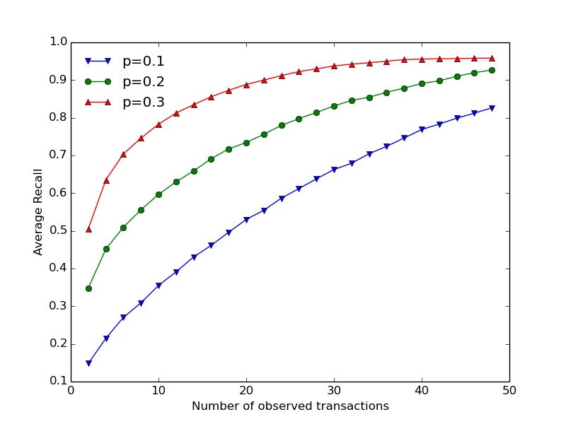
Figure 5. Recall vs. number of transactions per node in random $4$-regular graphs.

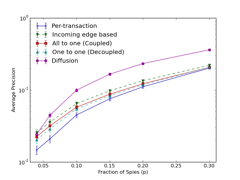
Figure 6. First-spy precision for 4-regular graphs under various forwarding schemes.

This result says that precision under the first-spy estimator is within a constant factor of optimal ($p^{2}$ is a fundamental lower bound on the maximum expected precision of any scheme (Bojja Venkatakrishnan et al., 2017)). Thus the precision gain from line graphs to 4-regular graphs is indeed small, as Figure 3 suggests. These observations motivate the use of 4-regular graphs, specifically in lieu of higher-degree regular graphs. First, 4-regular graphs have similar precision to complete graphs when the graph is known (i.e., the red dotted line is close to the middle black solid line, which is a lower bound on precision for regular graphs), but they sacrifice minimal precision when the graph is unknown. Hence, they provide robustness to graph-learning.

Lesson: 4-regular anonymity graphs provide more robustness to graph-learning attacks than line graphs.

Note that constructing an exact 4-regular graph with a fully-distributed protocol is difficult in practice; we will discuss how to construct an approximate 4-regular graph in §4.3, and how this approximation affects our anonymity guarantees.

4.2. Intersection Attacks

The previous section showed that $4$-regular graphs are robust to deanonymization attacks, even when the adversary knows the graph. However, those results assume that each user generates exactly one transaction per epoch. In this section, we relax the one-transaction-per-node assumption, and allow nodes to generate an arbitrary number of transactions. Dandelion  specifies that each transaction should take an independent path over the anonymity graph. In our case, this implies that if a node generates multiple transactions, each one will traverse a random walk (of geometrically-distributed length) over a 4-regular digraph. Under such a model, adversaries can aggregate metadata from multiple, linked transactions to launch intersection attacks. We first demonstrate Dandelion’s vulnerability to intersection attacks, and then provide an alternative propagation technique.

Attack. Suppose the adversary knows the graph. For each honest source $v\in V_{H}$, each of its transactions will reach one of the $np$ spy nodes first. In particular, each spy node has some fixed probability of being the first spy for transactions originating at $v$, given a fixed graph topology. We let $\Psi_{v}$ denote the pmf of the first spy for transactions starting at $v$; the support of this distribution is the set of all spies. We hypothesize that in realistic graphs, for $v\neq w$, $\Psi_{v}\neq\Psi_{w}$.

This hypothesis suggests a natural attack, which consists of a training phase and a test phase. In the training phase, for each candidate source, the adversary simulates dandelion spreading $N$ times. The resulting empirical distribution of first-spies for a given source determines the adversary’s estimate of $\Psi_{v}$. The adversary computes such a signature for each candidate source.

At testing, the adversary gets to observe $m$ transactions from a given node, $m\ll N$. The adversary again computes the empirical distribution $\hat{\Psi}$ of first-spies from those $m$ observations. The adversary then classifies $\hat{\Psi}$ to one of the $|V_{H}|$ classes (i.e., source nodes) by matching $\hat{\Psi}$ to the closest $\Psi_{i}$ from training. For each trial, $\hat{\Psi}$ and $\Psi_{v}$ are matched by maximizing the likelihood of signatures (i.e. by minimizing the KL divergence).

Figure 6 shows the recall for such an attack on a $4$-regular graph of size $1000$ with various fractions of spies, as a function of the number of transactions observed per node. By observing $10$ transactions per node, the recall exceeds $0.8$ when 30% of nodes are adversarial. This suggests that independent random forwarding leads to serious intersection attacks. Hence, a naive implementation of Dandelion critically damages anonymity properties.

Solution. To address these attacks, we consider forwarding mechanisms with correlated randomness. The key insight is that messages from the same source should traverse the same path; this prevents adversaries from learning additional information from multiple transactions. However, a naive implementation (e.g., adding a tag that identifies transactions from the same source, and sending all such transactions over the same path) makes it trivial to infer that otherwise unlinkable transactions originate from a common source. Hence, we consider three forwarding schemes that pseudorandomize the forwarding trajectory. In “one-to-one” forwarding, each node maps each of its inbound edges to a unique outbound edge; messages in stem mode only get relayed according to this mapping (Fig. 6). This one-to-one forwarding captures the ‘cable’ behavior described in Figure 2. Each node also chooses exactly one outbound edge for all of its own transactions. Here we randomize not by source, but by incoming edge (for relayed transactions). Similarly, “all-to-one” forwarding maps all inbound edges to the same outbound edge, and “per-incoming-edge” forwarding maps each inbound edge to a uniform outbound edge (with replacement).

Perhaps counterintuitively, these spreading mechanisms alter the anonymity guarantees even when the graph is unknown. Our next result—the second main theoretical contribution of this paper—suggests that one-to-one forwarding has near-optimal precision when the adversary does not know the graph, even in the face of intersection attacks (recall the lower bound of $p^{2}$, where $p$ is the fraction of spies (Bojja Venkatakrishnan et al., 2017)). The other two mechanisms do not.

Theorem 2.

Suppose the graph is unknown to the adversary, each node generates an arbitrary number of transactions, and the adversary can link transactions from the same user. The expected precision of the precision-optimal estimator for the one-to-one ($\mathbf{D}_{\mathtt{OPT-OtO}}$), all-to-one ($\mathbf{D}_{\mathtt{OPT-AtO}}$), and per-incoming-edge ($\mathbf{D}_{\mathtt{OPT-PIE}}$) message forwarding schemes are:

(3) $$\mathbf{D}_{\mathtt{OPT-OtO}} = \Theta\Big{(}p^{2}\log\Big{(}\frac{1}{p}\Big{)}\Big{)}$$

(4) $$\mathbf{D}_{\mathtt{OPT-AtO}} = \Theta(p)$$

(5) $$\mathbf{D}_{\mathtt{OPT-PIE}} = \Omega(p).$$

(Proof in Appendix B.2) This analysis exploits the tree-like neighborhoods of random 4-regular graphs. We first build a branching process that captures each routing mechanism, and then analyze the precision-optimal estimators accordingly.

Figure 6 illustrates simulated first spy precision values for each of these techniques, as well as diffusion (the status quo). Simulations were again run on a 100-node graph with an exact 4-regular topology; spies and sources were selected uniformly at random. ‘Per-transaction’ forwarding denotes the baseline i.i.d. random forwarding. This figure is plotted for the special case of one transaction per node; if nodes were to generate arbitrarily many transactions, the pseudorandom lines would stay the same (all-to-one, one-to-one, and per-incoming-edge), whereas Figure 6 suggests that the per-transaction curve could increase arbitrarily close to 1. The same is true for diffusion, as illustrated in prior work (Wang et al., 2014). In addition, when the graph is unknown and there is only one transaction per node, Figure 6 suggests that one-to-one forwarding achieves precision values that are close to the lower bound of per-transaction forwarding. The following corollary bounds the jump in precision when the graph is known to the adversary.

Proposition 1.

If the adversary knows the graph and internal routing decisions, then the precision-optimal estimator for one-to-one forwarding has an expected precision of $O(p)$.

(Proof in Appendix B.3)

An adversary that does not know internal forwarding decisions for all nodes has lower precision, because it must disambiguate between exponentially many paths for each transaction. Despite requiring completely new analysis, the 4-regular graph results for Theorem 2 and Proposition 1 are order-equivalent to the line graph results in (Bojja Venkatakrishnan et al., 2017). This raises an important question: are 4-regular graphs really better than line graphs? In an asymptotic sense, no. However, in practice, the story is more nuanced, and depends on the adversarial model. For adversaries that lack complete knowledge of the graph and each node’s routing decisions, we observe constant-order benefits, which become more pronounced once we take into account the realities of approximating 4- and 2- regular graphs. This is explored in §4.3. However, when the adversary has full knowledge of the graph and each node’s internal, random routing decisions, the combination of 4-regular graphs and one-to-one routing has slightly higher (worse) precision than a line graph. We detail this tradeoff in Appendix C. Another issue to consider is that line graphs do not help the adversary link transactions from the same source; meanwhile, on a 4-regular graph with one-to-one routing, two transactions from the same source in the same epoch will traverse the same path—a fact that may help the adversary link transactions.

Hence we recommend making the design decision between 4-regular graphs and line graphs based on the priorities of the system builders. If linkability of transactions is a first-order concern, then line graphs may be a better choice. Otherwise, we find that 4-regular graphs can give constant-order privacy benefits against adversaries with knowledge of the graph. Overall, both choices provide significantly better privacy guarantees than the current diffusion mechanism. We also want to highlight that the remaining sections of this paper are agnostic to the choice of graph topology; the lessons apply equally whether one uses a 4-regular graph or a line graph.

Lessons. If running Dandelion spreading over a 4-regular graph, use pseudorandom, one-to-one forwarding. If linkability of transactions is a first-order concern, then line graphs may be a more suitable choice.

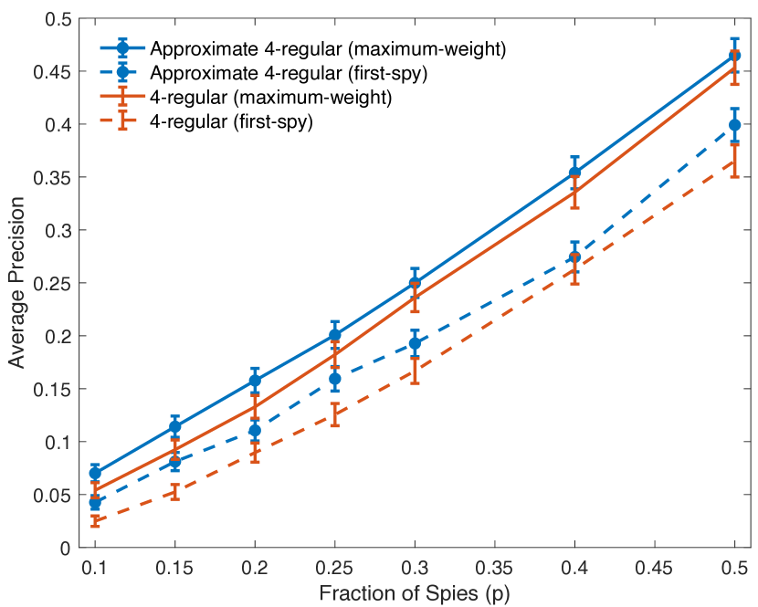
Figure 7. Average precision for approximate 4-regular graphs compared to exact 4-regular graphs.

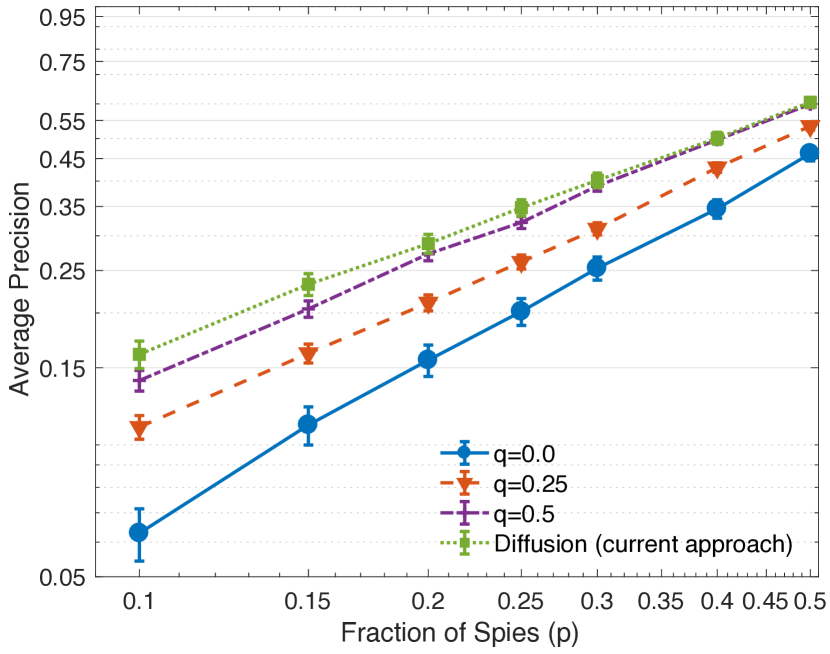
Figure 8. Honest-but-curious spies obey graph construction protocol.

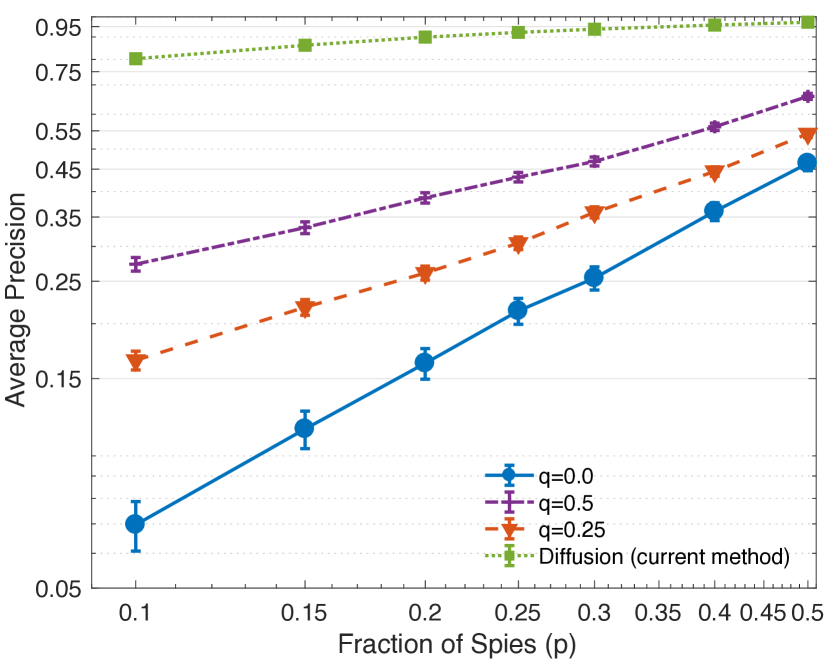
Figure 9. Malicious spies make outbound edges to every honest node.

4.3. Graph-Construction Attacks

We have so far considered graph-learning attacks and intersection attacks. Another important aspect of Dandelion++ is the anonymity graph construction, which should be fully distributed. Dandelion proposed an interactive, distributed algorithm (explained below) that constructs a randomized approximate line graph. In this section, we study how Byzantine nodes can change the graph to boost their accuracy. First, we show how to generate 4-regular graphs in the presence of Byzantine nodes. Next, we show how to choose $q$ (path length parameter) for robustness against Byzantine nodes.

4.3.1. Graph construction in Dandelion (Bojja Venkatakrishnan et al., 2017)

For any integral parameter $\ell>0$, Dandelion uses the protocol ApxLine($\ell$) to build a $\ell$-approximate line graph as follows: (1) Each node contacts $\ell$ random candidate neighbors, and asks for their current in-degrees. (2) The node makes an outbound connection to the candidate with the smallest in-degree. Ties are broken at random. This protocol is simple, distributed, and allows the graph to be periodically rebuilt. Though the resulting graph need not be an exact line, nodes have an expected degree of two, and experiments show low precision for adversaries. Increasing $\ell$ also enhances the likeness of the graph to a line and reduces the expected precision in simulation.

4.3.2. Construction of $4$-regular graphs.

A natural extension of Dandelion’s graph-construction protocol to 4-regular graphs involves repeating ApxLine($\ell$) twice for parameter $\ell>0$. That is, each peer makes two outgoing edges, where the target of each edge is chosen according to ApxLine($\ell$). As in the approximate line algorithm, the resulting graph is not exactly regular. However, the expected node degree is 4, and because each node generates two outgoing edges, the resulting graph has no leaves. This improves anonymity because leaf nodes are known to degrade average precision (Bojja Venkatakrishnan et al., 2017).

4.3.3. The impact of Byzantine nodes

Byzantine nodes can misbehave as recipients and/or creators of edges. As recipients, nodes can lie about their in-degrees during the degree-checking phase. As creators of edges, misbehaving nodes can generate many edges, even connecting to each honest node.

Lying about in-degrees. In step (1) of the graph-construction protocol, when a user queries an adversarial neighbor for its current in-degree, the adversary might deliberately report a lower degree than its actual degree. This can cause the querying user to falsely underestimate the neighbor’s in-degree and make a connection. In the extreme case, the adversarial node can consistently report an in-degree of zero, thus attracting many incoming edges from honest nodes. This degrades anonymity by increasing the likelihood of honest nodes passing their transactions directly to the adversary in the first hop. We find experimentally that such attacks significantly increase precision as $\ell$ grows; plots are omitted due to space constraints.

To avoid nodes lying about their in-degrees, we abandon the interactive aspect of Dandelion graph construction. In ApxLine(1), users select a random peer and make an edge regardless of the recipient’s in-degree. We therefore run ApxLine(1) twice, as shown in Algorithm 2. Note that Algorithm 2 closely mirrors the graph construction protocol used in Bitcoin’s P2P network today, so the protocol itself is not novel. In the line graphs of Dandelion, a higher $\ell$ value was needed since ApxLine($\ell$) for $\ell=1$ was shown to have significantly worse anonymity performance than $\ell\geq 2$. However such a loss is avoided in Dandelion++ since the application of ApxLine(1) twice eliminates leaves.

What is not previously known is how the approximate-regular construction in Algorithm 2 affects anonymity compared to an exact 4-regular topology. First, note that the expected recall does not change because dandelion spreading (Algorithm 4) has an optimally-low maximum recall of $p+O(\frac{1}{n})$, regardless of the underlying graph (Thm. 4, (Bojja Venkatakrishnan et al., 2017)). Hence, we wish to understand the effect of approximate regularity on maximum expected precision. We simulated dandelion spreading on approximate 4-regular graphs and exact 4-regular graphs, using the same approximate precision-optimal estimator from Figure 3. For comparison, we have also included the first-spy estimator. Figure 9 shows that the difference in precision between 4-regular graphs and approximate 4-regular graphs (computed with Algorithm 2) is less than 0.02 across a wide range of spy fractions $p$. Compared to line graphs (Bojja Venkatakrishnan et al., 2017, Figure 8), 4-regular graphs appear significantly more robust to irregularities in the graph construction.

Input: Set $V=\{v_{1},v_{2},\ldots,v_{n}\}$ of nodes;

Output: A connected, directed anonymity graph $H(V,E)$ with average degree $4$

for $v\leftarrow V$ do

       /* pick two random targets */

       $u_{1}\sim$ Unif$(V\setminus\{v\})$

       $u_{2}\sim$ Unif$(V\setminus\{v,u_{1}\})$

       /* make connections */

       $E=E\cup(v\rightarrow u_{1})\cup(v\rightarrow u_{2})$

end for

return $H(V,E)$

Algorithm 2 Approximate 4-Regular Graph Approximates a directed 4-regular graph in a fully-distributed fashion.

Creating many edges. Dandelion is naturally robust to nodes that create a disproportionate number of edges, because spies can only create outbound edges to honest nodes. This matters because in the stem phase, honest nodes only forward messages on outbound edges.

Proposition 2.

Consider dandelion spreading (Algorithm 4) with $q=0$ over a connected anonymity graph $H$ constructed according to graph-construction policy $\mathcal{P}$ (Algorithm 1). Let $\mathbf{D}_{\mathtt{OPT}}(\mathcal{P})$ and $\mathbf{R}_{\mathtt{OPT}}(\mathcal{P})$ denote the maximum expected precision and recall over graphs constructed according to $\mathcal{P}$. Now consider an alternative policy $\mathcal{Q}$ that is identical to $\mathcal{P}$ except adversarial nodes are allowed to choose their outbound edges arbitrarily. Let $\mathbf{D}_{\mathtt{OPT}}(\mathcal{Q})$ and $\mathbf{R}_{\mathtt{OPT}}(\mathcal{Q})$ denote the maximum expected precision and recall over all graphs constructed according to $\mathcal{Q}$. Then

$$\mathbf{R}_{\mathtt{OPT}}(\mathcal{Q}) = \mathbf{R}_{\mathtt{OPT}}(\mathcal{P})$$

(6) $$\mathbf{D}_{\mathtt{OPT}}(\mathcal{Q}) = \mathbf{D}_{\mathtt{OPT}}(\mathcal{P}).$$

(Proof in Appendix B.4).   This result bounds the deanonymization abilities of Byzantine nodes in general and supernodes in particular (Biryukov et al., 2014; Koshy et al., 2014), neither of which was covered by the analysis of (Bojja Venkatakrishnan et al., 2017). It shows that for the special case where the transition probability from stem to fluff phase $q=0$ (i.e., infinite stem phase), supernodes gain no deanonymization power by connecting to most or all of the honest nodes. In practice, we need $q>0$ to reduce broadcast latency, but analyzing this requires an upper bound on the probability of detecting the source of a diffusion process under sampled timestamp observations—a known open problem (Pinto et al., 2012; Zhu and Ying, 2014). We therefore simulate precision for nonzero $q$ as a function of spy fraction $p$, when spies obey protocol (Figure 9) and when they form outbound edges to all honest nodes (Figure 9). We generate a P2P graph via Algorithm 1 with out-degree $\eta=8$, and an anonymity graph $H$ via Algorithm 2, except spies form outbound edges to all honest nodes.

Figures 9 and 9 highlights two points: First, even when spies follow protocol, increasing $q$ increases precision. $q$ has the largest effect when $p$ is small; when $p=0.1$, using $q=0.5$ increases the expected precision by about 0.1 compared to $q=0.0$. For $q\leq 0.2$, we expect increases in precision on the order of 0.05. Second, spies can increase their precision by adding outbound edges; when $p=0.1$ and $q=0.5$, we observe a precision increase of about 0.2. Thus by choosing parameter $q\leq 0.2$, we can limit the increase in average precision to 0.1, even when spies connect to every honest node.

Lesson. To defend against graph-manipulation attacks, use noninteractive protocols and small $q$.

4.4. Black-Hole Attacks

Since dandelion spreading forwards messages to exactly one neighbor in each hop, propagation can terminate entirely if an adversarial relay in the stem chooses not to forward a message; we refer to this as a black-hole attack. To prevent black-hole attacks, Dandelion++  sets a random expiration timer at each stem relay immediately upon receiving transaction messages. If the relay does not receive an INV (i.e. an advertisement) for the transaction before his timer expires, then the relay diffuses the transaction. This policy provides a two-fold advantage over Dandelion: (1) messages are guaranteed to eventually propagate through the network, and (2) the random timers can help anonymize peers initiating the spreading phase in the event of a black-hole attack.

To implement this, Dandelion++ nodes are initialized with a timeout parameter $T_{\mathrm{base}}$. In the stem phase, when a relay $v$ receives a transaction, it sets an expiration time $T_{\mathrm{out}}(v)$:

(7) $$T_{\mathrm{out}}(v)\sim\text{{current\_time}}+\exp(1/T_{\mathrm{base}}),$$

i.i.d. across relays. If the transaction is not received again by relay $v$ before $T_{\mathrm{out}}(v)$, $v$ broadcasts the message using diffusion. Pseudocode is shown in Algorithm 5 (Appendix A).

Algorithm 5 solves the problem of message stalling, as relays independently broadcast if they have not received the message within a certain time. However, the protocol also ensures that the first relay node to broadcast is approximately uniformly selected among all relays that have received the message. This is due to the memorylessness of the exponential clocks: conditioned on a given node blocking the message, each of the remaining clocks can be reset assuming propagation latency in the stem is negligible. Ideally, the exponential clocks should be slow enough that they only trigger (with high probability) during a black-hole attack. On the other hand, they must also be fast enough to keep propagation latency low. This trade-off is analyzed in the following proposition.

Proposition 3.

For a timeout parameter $T_{\mathrm{base}}\geq\frac{-k(k-1)\delta_{\mathrm{hop}}}{2\log(1-\epsilon)}$, where $k,\epsilon$ are parameters and $\delta_{\mathrm{hop}}$ is the time between each hop (e.g., network and/or internal node latency), transactions travel for $k$ hops without any peer initiating diffusion with a probability of at least $1-\epsilon$.

(Proof in Appendix B.5)   Let $\Delta_{1}\triangleq k\delta_{\mathrm{hop}}$ be the time taken for the message to traverse $k$ hops. Conditioned on reaching $k$ hops and stalling, let $\Delta_{2}$ denote the additional time taken for the message to start diffusion. Then, $\Delta_{2}$ is the minimum of exponential random variables each of rate $1/T_{\mathrm{base}}$. As such $\Delta_{2}$ is itself exponentially distributed with rate $k/T_{\mathrm{base}}$. Choosing $T_{\mathrm{base}}$ as in Proposition 3, the mean additional time taken to diffuse the message is

(8) $$\mathbb{E}[\Delta_{2}]=\frac{T_{\mathrm{base}}}{k}=\frac{-(k-1)\delta_{\mathrm{hop}}}{2\log(1-\epsilon)}\leq\frac{-\Delta_{1}}{2\log(1-\epsilon)}\approx\frac{\Delta_{1}}{2\epsilon}.$$

The standard deviation of $\Delta_{2}$ is identical to the mean. Thus by choosing $T_{\mathrm{base}}$ as in Proposition 3 in Algorithm 5 we incur an additional delay at most a constant factor $1/(2\epsilon)$ from our delay $\Delta_{1}$ otherwise.

Lesson. Use random timers selected according to Prop. 3.

4.5. Partial-Deployment Attacks

The original Dandelion analysis does not consider the fact that instantaneous, full-network deployment of Dandelion++ is practically infeasible. In this section, we show that if implemented naively, Byzantine nodes can exploit partial Dandelion deployment to launch serious anonymity attacks. We also demonstrate a (counterintuitive) implementation mechanism that neutralizes this threat. We consider two natural approaches for constructing the anonymity graph.

Input: Main (directed) P2P graph $G(V,E)$, desired degree $d$ of output anonymity graph

Output: Directed anonymity graph $H(V,\tilde{E})$

for $v\in V$ do

       /* Find TwistedPair neighbors */

       $\mathcal{D}_{v}\leftarrow\{w\in\mathcal{N}_{out}(G,v)~{}|~{}w\text{ supports {\sc Dandelion++}}\}$

       if $0\leq|\mathcal{D}_{v}|<\frac{d}{2}$ then

             $\tilde{E}\leftarrow\tilde{E}\cup\mathcal{D}_{v}$

       end if

      /* Non-TwistedPair neighbors */

       if $|\mathcal{D}_{v}|==0$ then

             $\mathcal{R}\leftarrow\frac{d}{2}$ nodes drawn uniformly from $\mathcal{N}_{out}(G,v)$, without replacement

             $\tilde{E}\leftarrow\tilde{E}\cup\mathcal{R}$

       end if

      

end for

Algorithm 3 Version-checking. $\mathcal{N}_{out}(G,v)$ denotes the out-neighbors of node $v$ on digraph $G$.

Version-checking (Algorithm 3) generates an anonymity graph from edges between Dandelion++-compatible nodes. Each node $v$ first identifies its outbound peers on the main P2P network that support Dandelion++; we call this set $\mathcal{D}_{v}$. $\mathcal{D}_{v}$ can be learned from existing signaling in Bitcoin’s version handshake. Next, $v$ runs Algorithm 2, drawing candidate neighbors only from $\mathcal{D}_{v}$. If $|\mathcal{D}_{v}|=1$, $v$ uses the single node in $\mathcal{D}_{v}$ as its outbound anonymity graph edge. If $|\mathcal{D}_{v}|=0$, $v$ picks $2$ outbound neighbors uniformly at random, and uses them as anonymity graph edges. Upon forwarding a transaction to a node that does not support Dandelion++, the receiving node will, by default, relay the message using diffusion, thereby ending the stem phase. While version checking is a natural strategy, adversarial nodes can lie about their version number and/or run nodes that support Dandelion++.

Under the second approach, no-version-checking, each node $v$ instead selects $2$ outgoing edges uniformly from the set of all outgoing edges, without considering Dandelion++-compatibility. This noninteractive protocol shortens the expected length of the stem, thereby potentially weakening anonymity guarantees.

If all nodes supported Dandelion++, these two approaches would be identical. To model gradual deployment, we assume that all spy nodes run Dandelion++, and a fraction $\beta$ of the remaining honest nodes are using Dandelion++. Honest users are distributed uniformly over the network. Let $V_{D}$ denote the nodes that support Dandelion++: $|V_{D}|=pn+(1-p)\beta n$. We wish to characterize the maximum expected recall of Dandelion++  as a function of $p$ and $\beta$, for version-checking and no-version-checking. The following theorem bounds this quantity under a recall-optimal estimator.

Theorem 3.

Consider $n$ nodes in an approximately-$2\eta$-regular graph $G$ generated according to Algorithm 1. A fraction $p$ of nodes are spies running Dandelion++. Among the remaining honest nodes, a fraction $\beta$ support Dandelion++. Under version-checking, the expected recall across honest, Dandelion++-compatible nodes, under a recall-optimal mapping strategy satisfies

(9) $$\frac{p}{f}\left(1-(1-f)^{\eta}\right)\leq\mathbf{R}_{\mathtt{OPT}}\lesssim \frac{p}{f}\left(1-(1-f)^{\eta}\right)+(1-f)^{\eta}+C(1-\beta))$$

where $f$ is the fraction of all nodes that support Dandelion++  and $C=\left(1-\frac{p}{f}\right)\left(1-\left(1-f\right)^{\eta}\right)\frac{1-(1-\phi)^{\tilde{n}}}{\tilde{n}\phi}$, where $\phi=1-(1-\frac{1}{n-\eta})^{\eta}$, and $\tilde{n}=(1-p)n$ is the number of honest nodes in the system. Under no-version-checking,

(10) $$p\leq\mathbf{R}_{\mathtt{OPT}} \lesssim p+(1-\beta(1-q))(1-p)\frac{1-(1-\phi)^{\tilde{n}}}{\tilde{n}\phi}.$$

(Proof in Appendix B.6)   Here $\lesssim$ denotes approximate inequality; i.e., $A(n)\lesssim B(n)$ implies that there exist constants $n_{0}>0$ and $C^{\prime}>0$ such that for all $n>n_{0}$, $A(n)\leq C^{\prime}B(n)$. In this case, such a condition holds for any $C^{\prime}>1$.

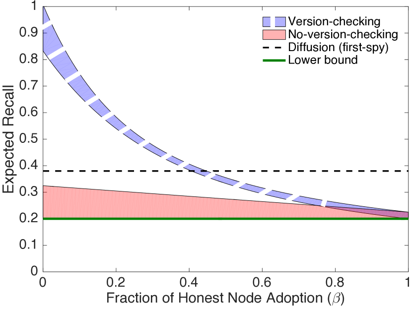
Figure 10. Bounds on maximum expected recall for $p=q=0.2$ and $n=1000$, on an approximately-16-regular graph.

Figure 11. Time to propagate to 10% of the network as a function of the path length. Blue is the line of best fit at 218ms per hop, and green is the minimum estimated delay at 300ms per hop.

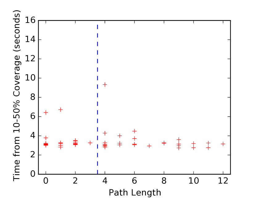
Figure 12. Time to go from 10% to 50% of the network. The blue line indicated where data was split into two categories by hop length with almost equal numbers of samples (low: 26, high: 29).

Figure 12 plots these results for $p=0.2$ fraction of spies and $q=0.2$ probability of ending the Dandelion++ stem, on an approximately-16-regular P2P graph. Our theoretical bounds delimit the shaded regions; for comparison, we include a lower bound on the recall of diffusion, computed by simulating diffusion with a first-spy estimator. The green solid line is a lower bound on the maximum expected recall of any spreading protocol (Thm. 2, (Bojja Venkatakrishnan et al., 2017)). When $\beta$ is small, version-checking recall is close to 1; in the same regime, no-version-checking exhibits lower recall than both diffusion and version-checking. Intuitively, when adoption is low (low $\beta$), any Dandelion++ peers are likely to be spies. Therefore, version-checking actually increases the likelihood of getting deanonymized. In the same low-$\beta$ regime, no-version-checking is more likely to choose a Dandelion++-incompatible node $w$ as the next stem node. While this prematurely ends the stem, it still introduces more uncertainty than vanilla diffusion.

Lesson. Use no-version-checking to construct the graph.

5. Evaluation

5.1. Implementation in Bitcoin

We have developed a prototype implementation of Dandelion++. Our prototype is a modification of Bitcoin Core (referred to as Core from now on), the most commonly-used client implementation in the Bitcoin network. In total, our implementation required a patch modifying approximately 500 lines of code. A vital part of our implementation is allowing nodes to recognize other Dandelion++  nodes in a straightforward way. In Core, supported features are signaled by modifying the nServices field in the handshake. For example, segwit support is signalled by setting bit $4$ in nServices. In our case, Dandelion++  support is signaled by setting the $25$th bit.

To minimize our footprint on the Core codebase, we insert Dandelion++  functionality into the preexisting main threads/signals that handle the processing and transmission of messages. However, creating the $4$-regular anonymity graph and processing Dandelion++  transactions requires careful consideration of the many concurrency and DoS-protection mechanisms already at play in Core. For instance, Core’s data structures for transactions and inventory messages are designed to facilitate responses to GetData requests, while broadcasting transactions to all nodes with exponential delays. These data structures are insufficient for Dandelion++  because they facilitate broadcasting knowledge of transaction and block hashes. In particular, Dandelion++  nodes need to hide knowledge of transactions that are still in the stem phase, but at the same time ensure that they are relayed properly and not stalled by adversaries. Our approach is to store stem mode transactions in an additional data structure, the “embargo map,” such that embargoed transactions are omitted from GetData responses. The embargo map serves two purposes: 1. it tracks transactions currently in the stem phase and 2. it ensures that malicious adversaries can not stop transaction propagation (§4.4).

5.2. Experimental Setup

We used our prototype implementation to conduct integration experiments, by launching our own nodes running the Dandelion++  software, and connecting to the actual Bitcoin network. The goal of our experiments is to characterize how Dandelion++  affects transaction propagation latency. The experiments also validate our implementation and its compatibility with the existing network.

For our experiments we launched 30 Dandelion instances of m3.medium Amazon EC2 nodes (t2.medium used in Seoul and Mumbai where m3.medium is not available). The nodes are spread geographically across 10 different AWS regions (California, Sydney, Tokyo, Frankfurt, etc.)—3 nodes per region (aws, [n. d.]). To control the topology between the Dandelion nodes, we use Core’s -connect or -addnode command line flags. Our measurements use the Coinscope (Miller et al., 2015) tool to connect to each node in the Bitcoin network and record a timestamped log of transaction propagation messages.

5.3. Evaluation Results

5.3.1. Propagation latency at fixed stem lengths

We conducted a preliminary experiment to inform our choice of the coin flip (stem length) parameter, $q$. In this experiment, we arranged our Dandelion++  nodes in a chain topology (each with one outgoing connection to the next, with the last node connected to the Bitcoin network) so that we could deterministically control the stem length. Based on 20 trials for stems up to length 12, we estimated that each additional hop adds an expected 300 miliseconds to the propagation latency. There is also a constant 2.5 second delay added to each transactions due to the exponential process of propagation when it first enters the fluff phase. Taking a propagation delay of 4.5 seconds as our goal, we chose $q=0.1$ or $q=0.2$ as our parameter (recall the expected stem length is $1/q$).

The observed delays originate from two main sources. First, each hop incurs network latency due to transit time between nodes. A recent measurement study of the Bitcoin network estimated a median latency of 110ms between nodes (Gencer and Sirer, 2017), and Bitcoin transaction propagation requires three messages (INV, GETDATA, TX). The latency between our EC2 nodes is faster, with a median of only 86ms across all pairs. Although our EC2 nodes are geographically distributed, they are closely connected to internet backbone endpoints. Second, Bitcoin Core buffers each Inv message for an average of 2.5 seconds; however, our implementation relays Dandelion++  transactions immediately, so internal node delays should be negligible. We therefore estimate 300 miliseconds of delay per stem node, which is consistent with our preliminary experiments.

5.3.2. Topology

In order to create a connected graph of Dandelion++  nodes, we use all of the eight outgoing connections from each of our nodes to connect to other Dandelion++  nodes. This ensures that we can measure many different stem lengths and how they affect the propagation to the rest of the network. We must also account for an artifact of our experiment setup, namely that short cycles in the stems are more likely among our 30 well connected Dandelion++  nodes . We therefore parse debug logs from our nodes for each trial in order to determine the effective stem length, which we then use as the basis of our evaluation.

In our experiment, we re-randomize the topology to avoid biasing our results. For each randomization of the connections, we generate 5 transactions, 10 seconds apart. We repeat this “burst” 4 times a day over three separate days. The transactions are injected into the network via a randomly-chosen node. We show the results of the experiment in Figures 12 and 12.

Figure 12 plots the time it takes Dandelion++  transactions to reach 10% of the network. As mentioned in Section 5.3.1, for every additional hop in the stem phase there is a minimum delay added by three messages and a expected delay of 2.5 seconds. The solid green line represents the minimum expected delay and the dotted blue line representst the best linear fit over the transaction data. The propagation delay to reach 10% coverage increases with the path length due to the minimum added delay. We also computed the two-sided Pearson Correlation Coefficient over the two variables: path length and time to reach 10%. The coefficient $r=0.292$ implies a small positive correlation between the two variables.

Figure 12 plots the the time it takes a transaction to go from 10% to 50% of the network with respect to the path length. Unlike the first scatter plot, visual inspection doesn’t reveal any relationship between the two variables in this case. This is also what we expect because Dandelion++  should not have any impact on transaction propagation after it has entered fluff phase. We also perform a Mann-Whitney U Test to test the null hypothesis: time from 10-50% coverage does not depend on path length. Using the path length as the independent variable, we split it into two categories: high and low. The blue dotted line in Figure 12 is the boundary of the two categories where there are 26 samples in “low” and 29 in “high”. The Mann Whitney U test gives a U statistic of 443 and a p-value of 0.269. This implies that there is weak evidence against the null hypothesis, therefore we fail to reject it.

As expected, the minimum delay brought on by Dandelion++  has a positive correlation with the time it takes to reach 10% of the Bitcoin network. Similarly, once a transaction has left the stem phase, it begins normal propagation through the network and is therefore no longer be affected by Dandelion++. This prediction is confirmed by our test of independence of hop length (high v. low) and time from 10-50% coverage.

6. Conclusion

A gap exists between the theory and practice of protecting user anonymity in cryptocurrency P2P networks. In particular, there are no safeguards against population-level deanonymization, which is the focus of this paper. We aim to narrow that gap by identifying strong or unrealistic assumptions in a state-of-the-art proposal (Bojja Venkatakrishnan et al., 2017), demonstrating the anonymity effects of violating those assumptions, and proposing lightweight, theoretically-justified fixes in the form of Dandelion++. This methodology complements the usual development pattern in cryptocurrencies, which has mainly evolved by applying ad hoc patches against specific attacks. We instead take a first-principles approach to design.

Note that Dandelion++ does not explicitly protect against ISP- or AS-level adversaries, which can deanonymize users through routing attacks (Apostolaki et al., 2016). Understanding how to analyze and protect against such attacks is of fundamental interest. However, Dandelion++ is already compatible with a number of the countermeasures proposed in (Apostolaki et al., 2016). For instance, (Apostolaki et al., 2016) proposes to enhance network diversity through multi-homing of nodes and routing-aware network connectivity. Such countermeasures directly support Dandelion++ by ensuring that nodes are less likely to establish outbound anonymity edges exclusively to spies.

Appendix A Algorithms

Dandelion pseudocode is presented in Algorithm 4. Pseudocode for handling black-hole attacks is included in Algorithm 5.

Input: Message $X_{v}$, source $v$, anonymity graph $H$, spreading graph $G$, parameter $q\in(0,1)$

anonPhase $\leftarrow$ True

head $\leftarrow v$

recipients $\leftarrow\{v\}$

while anonPhase do

       /* relay message to random node */

       target $\sim$ Unif$(\mathcal{N}_{out}(H,\text{head}))$

       recipients $\leftarrow$ recipients $\cup\{X_{v}\}$ from head to target

       head $\leftarrow$ target

       $u\sim$ Unif$([0,1])$

       if $u\leq q$ then

             anonPhase $\leftarrow$ False

            

       end if

      

end while

/* Run diffusion on $G$ from ‘head’ */

Diffusion$(X_{v},\text{head},G)$

Algorithm 4 Dandelion Spreading (Bojja Venkatakrishnan et al., 2017). $\mathcal{N}_{out}(G,v)$ denotes the out-neighbors of node $v$ on directed graph $G$.

Input: Message and timeout parameter $(X,T_{\mathrm{base}})$ received by $v$ in the anonymity phase, out-neighbors $\mathcal{N}_{out}(G,v)$ on anonymity graph $G$, spreading graph $H$, parameter $q\in(0,1)$

$T_{\mathrm{out}}(v)\sim\exp(1/T_{\mathrm{base}})$

  // set timer

forward $(X,T_{\mathrm{base}})$ according to dandelion

/* wait until message re-received */

while current_time $\leq T_{\mathrm{out}}$ do

       if $X$ received then

             timer $\leftarrow$ inactive

             break

            

       end if

      continue

      

end while

/* start diffusion */

if timer is active then

       Diffusion$(X,v,H)$

      

end if

Algorithm 5 Dandelion++  Spreading at node $v$. The protocol guarantees eventual network-wide propagation of transactions.

Appendix B Proofs

B.1. Proof Theorem 1

See 1

Proof.

Each node has two predecessors and two successors; let us arbitrarily label these as the left predecessor (successor) and the right predecessor (successor). For $i,j,k,l\in\{a,h\}$, let $\mathcal{E}_{v}(^{i,j}_{k,l})$ denote the event that $v$’s left successor, right successor, left predecessor and right predecessor are of types $i,j,k$ and $l$ respectively, where type of $a$ denotes an adversarial node and a type $h$ denotes an honest node. Also, assume that for any honest node $v\in V_{H}$ the number of messages forwarded by $v$ is statistically independent of the local neighborhood upstream of $v$. This assumption follows from the locally-tree-like nature of sparse random graphs (Mezard and Montanari, 2009). We use the following two lemmas, whose proofs are included below.

Lemma 0.

Let $J_{v}$ denote the number of transactions (from honest servers) that reach $v$ before reaching an adversary. Then, for each event $\mathcal{E}\in\{\mathcal{E}_{v}(^{a,h}_{h,h}),\mathcal{E}_{v}(^{h,a}_{h,h}),\mathcal{E}_{v}(^{h,h}_{a,h}),\mathcal{E}_{v}(^{h,h}_{h,a})\}$ $\mathbb{E}[\max_{x\in\mathcal{X}}\mathbb{P}(X_{v}=x|\mathbf{O},\mathcal{E},J_{v})|\mathcal{E},J_{v}]\leq\frac{1}{J_{v}+1}.$

Lemma 0.

For any server $v\in V_{H}$, let $F_{v}$ denote the number of transactions that (i) reach $v$ before reaching any adversary and (ii) are forwarded by $v$ along its left outgoing edge. Then $\mathbb{E}\left[\frac{1}{F_{v}+1}\right]\leq\frac{2\mathbf{D}_{\mathtt{FS}}(v)}{p}.$

Now, recall the events $\mathcal{E}_{v}(^{i,j}_{k,l})$, where $i,j,k,l\in\{a,h\}$. There are a total of $2^{4}=16$ such events that are possible for the neighborhood around server $v$. Out of these events, $\binom{4}{2}=6$ of them occur with a probability of $p^{2}(1-p)^{2}$ (such as $\mathcal{E}_{v}(^{a,a}_{h,h})$ for e.g.). Similarly $\binom{4}{3}=4$ events occur with a probability of $p^{3}(1-p)$ and one event occurs with a probability of $p^{4}$. Since the per-node precision can be at most 1, the above events contribute to a cumulative precision gain of at most $6p^{2}+4p^{3}+p^{4}$.

The remaining cases are events where only one neighbor is adversarial—$\mathcal{E}_{v}(^{a,h}_{h,h}),\mathcal{E}_{v}(^{h,a}_{h,h}),\mathcal{E}_{v}(^{h,h}_{a,h})$ and $\mathcal{E}_{v}(^{h,h}_{h,a})$—or when all of the neighbors are honest $\mathcal{E}_{v}(^{h,h}_{h,h})$. Note that each of these events occur with a probability of at least $p(1-p)^{3}$ and hence the trivial bound used above cannot be used here. Let us first consider the event $\mathcal{E}_{v}(^{h,h}_{a,h})$ where only the left predecessor node of $v$ is an adversary. Let $U\in V_{H}$ denote the right predecessor of $v$ and $F_{U}$ the number of fresh transactions that are forwarded by $U$ to $v$. Then from Lemma B.1 we have

$$\Rightarrow\sum_{f\geq 0}\mathbb{P}(F_{U}=f,\mathcal{E}_{v}(^{h,h}_{a,h}))\cdot$$

$$\mathbb{E}[\max_{x\in\mathcal{X}}\mathbb{P}(X_{v}=x|\mathbf{O},F_{U},\mathcal{E}_{v}(^{h,h}_{a,h}))|F_{U},\mathcal{E}_{v}(^{h,h}_{a,h})]$$

$$\leq\mathbb{P}(\mathcal{E}_{v}(^{h,h}_{a,h}))\mathbb{E}\left[\frac{1}{F_{U}+1}\right]\leq p\frac{2\mathbf{D}_{\mathtt{FS}}(v)}{p}=2\mathbf{D}_{\mathtt{FS}}(v).$$

where we use (a) the independence of $F_{U}$ and the local neighborhood upstream of $U$, and (b) Lemma B.2. By analogous arguments we can similarly bound the expected precision under events $\mathcal{E}_{v}(^{h,h}_{h,a}),\mathcal{E}_{v}(^{a,h}_{h,h})$ and $\mathcal{E}_{v}(^{h,a}_{h,h})$.

Finally consider $\mathcal{E}_{v}(^{h,h}_{h,h})$, in which case $v$’s location is completely hidden from the adversaries. Let $I$ be the set of such nodes. Since each adversary is a neighbor to at most 4 honest nodes, there are at least $\tilde{n}-4np=(1-5p)n$ nodes in $I$. So $\forall x\in\mathcal{X}$, we have $\mathbb{P}(X_{v}=x|\mathbf{O},G,I,\mathcal{E}_{v}(^{h,h}_{h,h}))$

(11) $$=\mathbb{P}(X_{v^{\prime}}=x|\mathbf{O},G,I,\mathcal{E}_{v}(^{h,h}_{h,h})) ~{}\forall v^{\prime}\in I$$

$$\Rightarrow\mathbb{P}(X_{v}=x|\mathbf{O},G,I,\mathcal{E}_{v}(^{h,h}_{h,h})) \leq\frac{1}{|I|}\leq\frac{1}{(1-5p)n}$$

(12) $$\Rightarrow\max_{x\in\mathcal{X}}\mathbb{P}(X_{v}=x|\mathbf{O},\mathcal{E}_{v}(^{h,h}_{h,h})) \leq\frac{1}{(1-5p)n},$$

and hence $\mathbb{E}[\max_{x\in\mathcal{X}}\mathbb{P}(X_{v}=x|\mathbf{O},\mathcal{E}_{v}(^{h,h}_{h,h}))|\mathcal{E}_{v}(^{h,h}_{h,h})]\leq\frac{1}{(1-5p)n}$. Summing over all the cases considered gives the result. ∎

B.1.1. Proof of Lemma B.1

See B.1

Proof.

W.l.o.g., let $U_{1},U_{2},\ldots,U_{J_{v}}$ be the servers whose transactions are received by $v$ and let $W_{v}=\{v,U_{1},U_{2},\ldots,U_{J_{v}}\}$. Consider any matching $\mathbf{x}$ where $x_{u}$ is the message assigned to server $u$. Then

(13) $$\mathbb{P}(\mathbf{S}|G,W_{v},\mathbf{X}=\mathbf{x})=\mathbb{P}(\mathbf{S}|G,W_{v},\mathbf{X}=\mathbf{x^{\prime}})$$

where $\mathbf{x^{\prime}}$ is a new assignment of messages such that $x^{\prime}_{u}=x_{u}$ for all $u\in V_{H},u\notin W_{v}$ and $x^{\prime}_{W_{v}}=x_{W_{v}}$. This implies, for any fixed $x\in\mathcal{X}$, $\mathbb{P}(X_{v}=x|\mathbf{O},\mathcal{E},J_{v},G,W_{v},X_{V_{H}\backslash W_{v}})=$

(14) $$= \frac{\mathbb{P}(X_{v}=x,\mathbf{O},X_{V_{H}\backslash W_{v}}|\mathcal{E},J_{v},G,W_{v})}{\mathbb{P}(\mathbf{O},X_{V_{H}\backslash W_{v}}|\mathcal{E},J_{v},G,W_{v})}$$

$$= \frac{\mathbb{P}(\mathbf{O}|\mathcal{E},J_{v},G,W_{v},X_{v}=x,X_{V_{H}\backslash W_{v}})}{\sum_{x^{\prime}}\mathbb{P}(\mathbf{O}|\mathcal{E},J_{v},G,W_{v},X_{v}=x^{\prime},X_{V_{H}\backslash W_{v}})}$$

$$\leq \frac{1}{J_{v}+1}$$

(15) $$\Rightarrow \mathbb{P}(X_{v}=x|\mathbf{O},\mathcal{E},J_{v})\leq\frac{1}{J_{v}+1}$$

$$\Rightarrow \max_{x\in\mathcal{X}}\mathbb{P}(X_{v}=x|\mathbf{O},\mathcal{E},J_{v})\leq\frac{1}{J_{v}+1}$$

$$\Rightarrow \mathbb{E}[\max_{x\in\mathcal{X}}\mathbb{P}(X_{v}=x|\mathbf{O},\mathcal{E},J_{v})|\mathcal{E},J_{v}]\leq\frac{1}{J_{v}+1}.$$

The claim follows. ∎

B.1.2. Proof of Lemma B.2

See B.2

Proof.

For server $v$, consider event $\mathcal{E}_{v}$ in which the node incident on $v$’s left outgoing edge is an adversary. Also, let $\mathcal{L}_{v}$ denote the event that $X_{v}$ is forwarded along $v$’s left outgoing edge. Then clearly,

(16) $$\mathbf{D}_{\mathtt{FS}}(v)\geq\mathbb{P}(\mathcal{E}_{v},\mathcal{L}_{v})\mathbb{E}[D_{\mathtt{FS}}(v)|\mathcal{E}_{v},\mathcal{L}_{v}]=\frac{p}{2}\mathbb{E}[D_{\mathtt{FS}}(v)|\mathcal{E}_{v},\mathcal{L}_{v}].$$

Now, from our assumption $F_{v}$ is independent of the events $\mathcal{E}_{v}$ and $\mathcal{L}_{v}$. In this case, the expected precision becomes $\mathbb{E}[D_{\mathtt{FS}}(v)|\mathcal{E}_{v},\mathcal{L}_{v}]=\mathbb{E}\left[\frac{1}{F_{v}+1}\bigg{|}\mathcal{E}_{v},\mathcal{L}_{v}\right]=\mathbb{E}\left[\frac{1}{F_{v}+1}\right]$, which combined with Equation (16) gives the lemma. ∎

B.2. Proof of Theorem 2

See 2

Proof.

We start with two lemmas that reduce the problem to a first-spy precision calculation.

Lemma 0 (Intersection).

Under each of the spreading mechanisms (all-to-one, one-to-one, and per-incoming-edge), the adversary’s maximum expected precision $\mathbf{D}_{\texttt{OPT}}$ is not a function of the number of transactions per node.

This proof follows directly from the pseudorandomness of the forwarding mechanisms, and is omitted for brevity.

Lemma 0 (First-Spy Optimality).

For all spreading mechanisms (all-to-one, one-to-one, and per-incoming-edge), there exists a constant $C$ such that $\mathbf{D}_{\texttt{OPT}}\leq C\cdot\mathbf{D}_{\texttt{FS}}+O(p^{2})$, where $\mathbf{D}_{\texttt{FS}}$ denotes the expected precision of the first-spy estimator.

Lemma B.4 is proved analogously to Theorem 1. The full proof is omitted for brevity. Together, lemmas B.3 and B.4 imply that to characterize the precision-optimal estimator, we can focus on the first-spy estimator. For brevity, we prove only all-to-one and one-to-one results in the following lemmas.

Lemma 0 (One-to-One First-Spy).

The expected precision of the first-spy estimator for one-to-one forwarding satisfies $\mathbf{D}_{\texttt{FS-OtO}}=O\Big{(}p^{2}\log\Big{(}\frac{1}{p}\Big{)}\Big{)}$.

Proof.

Let $v\in V_{H}$, and denote the vertex to which $v$ forwards its message $X_{v}$ as $s\in V$. In the case that $s\in V_{H}$ the precision of the first spy estimator for $v$ is $0$, because $X_{v}$ is never matched to $v$. When $s\in V_{A}$, the precision of the first spy estimator for $v$ is $\frac{1}{|W_{v}|}$, where $W_{v}$ denotes the set of nodes from which all fresh messages that $v$ transmits to $s$ originate. Note that $v\in W_{v}$. Now $\mathbb{E}[D_{\texttt{FS}}(v)]=\mathbb{P}(s\in V_{A})\mathbb{E}[\frac{1}{|W_{v}|}|s\in V_{A}]$, where $\mathbb{P}(s\in V_{A})=p$ and $\mathbb{E}\Big{[}\frac{1}{|W_{v}|}\Big{|}s\in V_{A}\Big{]}=\sum_{w=1}^{\infty}\mathbb{P}\big{(}|W_{v}|=w\big{|}s\in V_{A}\big{)}\frac{1}{w}$.

Lemma 0.

Under one-to-one forwarding, $\mathbb{P}\big{(}|W_{v}|=w\big{|}s\in V_{A}\big{)}=\frac{2p}{1-p}\Big{(}\frac{1-p}{1+p}\Big{)}^{w}.$

(Proof in Appendix B.2.1).

Using Lemma B.6 to expand the summation gives $\mathbb{E}\Big{[}\frac{1}{|W_{v}|}\Big{|}s\in V_{A}\Big{]}=\sum_{w=1}^{\infty}\frac{1}{w}\frac{2p}{1-p}\Big{(}\frac{1-p}{1+p}\Big{)}^{w}=\frac{-2p}{1-p}\log\Big{(}\frac{2p}{1+p}\Big{)}$. Thus, $\mathbb{E}\Big{[}\frac{1}{|W_{v}|}\Big{|}s\in V_{A}\Big{]}=\frac{2p}{1-p}\log\Big{(}\frac{1+p}{2p}\Big{)}$ and $\mathbb{E}[D_{\texttt{FS-OtO}}(v)]=\frac{2p^{2}}{1-p}\log\Big{(}\frac{1+p}{2p}\Big{)}.$ ∎

Lemma 0 (All-to-One First-Spy).

The expected precision of the first-spy estimator for all-to-one forwarding satisfies $\mathbf{D}_{\texttt{FS-AtO}}=\Theta(p)$.

Proof.

We demonstrate upper and a lower bounds on $\mathbf{D}_{\texttt{FS-AtO}}$. As before, these bounds are obtained by computing the expected precision of a given node $v\in V_{H}$, and we denote the node to which $v$ forwards its message $X_{v}$ as $s\in V$. Let $W_{v}$ be the set of nodes from which all fresh messages transmitted by $v$ to $s$ originate; our goal is to compute $\mathds{E}[\frac{1}{W_{v}}|s\in V_{A}]$.

Lower bound. We use the following lemma:

Lemma 0.

Under all-to-one forwarding, $\mathbb{P}\big{(}|W_{v}|=w\big{|}s\in V_{A}\big{)}=\frac{(2w)!}{(w+1)!w!}\Big{(}\frac{1-p}{2}\Big{)}^{w-1}\Big{(}\frac{1+p}{2}\Big{)}^{w+1}.$

(Proof in Appendix B.2.2).

Note that $\mathbb{E}\Big{[}\frac{1}{|W_{v}|}\Big{|}s\in V_{A}\Big{]}=\sum_{w=1}^{\infty}\mathbb{P}\big{(}|W_{v}|=w\big{|}s\in V_{A}\big{)}\frac{1}{w}$. We can lower bound this summation by computing only the first term using Lemma B.8. This gives $\mathbb{P}(|W_{v}|=1|s\in V_{A})=\frac{1}{4}p^{2}+\frac{1}{2}p+\frac{1}{4}$. Hence $\mathbb{E}[D_{\texttt{FS}}(v)]=\mathbb{P}(s\in V_{A})\mathbb{E}[\frac{1}{|W_{v}|}|s\in V_{A}]\geq\frac{p}{4}+O(p^{2})$, or $\mathbb{E}[D_{\texttt{FS}}(v)]=\Omega(p)$.

Upper bound. Due to the branching properties of all-to-one forwarding, we now model $v$’s upstream neighborhood (i.e. nodes that can send transactions to $v$) as a Galton-Watson (GW) branching process (Athreya and Ney, 2004). This modeling assumption is appropriate as $n\rightarrow\infty$ due to the locally-tree-like properties of sparse random graphs (Mezard and Montanari, 2009).

Each node in a realization of the GW process is a viable candidate source whose own transactions could reach $v$. The branching distribution of the process is therefore determined by the fraction of spies $p$, and the forwarding mechanism (in this case, all-to-one). $W_{v}$ is the number of nodes in this tree.

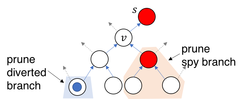
Figure 13. Branching process model of upstream neighborhood. Red nodes are spies; blue dots denote nodes that divert their transactions out of the tree. Both events result in pruning.

Figure 13 illustrates this model. Suppose we start with a binary tree rooted at $v$—this includes the entire upstream anonymity graph with respect to $v$. Each node has a second outbound edge (dashed grey line); due to our locally-tree-like assumption, those edges cannot be used to reach $v$, and are not part of the branching process. If a node is a spy, the spy and its upstream ancestors get pruned from the tree. Similarly, if a node chooses to forward its incoming messages along the grey edge, then none of its upstream children’s transactions will reach $v$; hence we prune the node and its ancestors. We let $\nu$ denote the probability that a node is a spy or forwards its transactions on its grey edge, $\nu=\frac{1}{2}(1+p)$. The mean of this offspring distribution $\mu=2(1-\nu)=1-p<1$ for $p\neq 0$, so this GW process is subcritical and goes extinct with probability 1 (Athreya and Ney, 2004). Hence we can focus our analysis on trees of finite size. We use Lemma B.8 to expand $\mathbb{E}\Big{[}\frac{1}{|W_{v}|}\Big{|}s\in V_{A}\Big{]}=$

(17) $$= \sum_{w=1}^{\infty}\frac{1}{w}\frac{(2w)!}{(w+1)!w!}(\frac{1-p}{2})^{w-1}(\frac{1+p}{2})^{w+1}$$

$$= \frac{1}{4}(1+p)^{2}\sum_{w=1}^{\infty}\frac{1}{w}\frac{2e^{2}}{\pi}\frac{1}{w+1}4^{w-1}\big{(}\frac{1}{4}(1-p^{2})\big{)}^{w-1}.$$

where (17) uses Stirling’s inequalities. For $p\in[0,1]$, $\sum_{w=1}^{\infty}\frac{(1-p^{2})^{w-1}}{w(w+1)}\leq\sum_{w=1}^{\infty}\frac{1}{w(w+1)}=1$. Thus, $\mathbb{E}\Big{[}\frac{1}{|W_{v}|}\Big{|}s\in V_{A}\Big{]}\leq\frac{e^{2}}{2\pi}(1+p)^{2}$ and $\mathbf{D}_{\texttt{FS-AtO}}\leq\frac{e^{2}}{2\pi}p+O(p^{2}).$ ∎

∎

B.2.1. Proof of Lemma B.6

See B.6

Proof.

Under one-to-one forwarding, all messages other than $X_{v}$ transmitted by $v$ to $s$ are received by $v$ from the same predecessor $v^{\prime}$. Likewise, all messages transmitted by $v^{\prime}$ to $v$ are received by $v^{\prime}$ from the same predecessor $v^{\prime\prime}$ (other than $X_{v^{\prime}}$ in the case that $X_{v^{\prime}}$ is transmitted to $v$). Continuing this reasoning results in a line graph of predecessor nodes. Note that the first adversary predecessor node in this line graph prevents any subsequent predecessors from contributing to $W_{v}$. We condition on $|T|$, the number of vertices in the line graph: $\mathbb{P}\big{(}|W_{v}|=w\big{|}s\in V_{A}\big{)}=\sum_{t=w}^{\infty}\mathbb{P}\big{(}|T|=t\big{|}s\in V_{A}\big{)}\mathbb{P}\big{(}|W_{v}|=w\big{|}|T|=t,s\in V_{A}\big{)}.$ Here, $\mathbb{P}\big{(}|T|=t\big{|}s\in V_{A}\big{)}=p(1-p)^{t-1}$ (recall that $v$ is a member of $T$ with probability $1$). Additionally, $\mathbb{P}\big{(}|W_{v}|=w\big{|}|T|=t,s\in V_{A}\big{)}={t-1\choose w-1}(\frac{1}{2})^{w-1}(\frac{1}{2})^{t-w}$. Therefore, $\mathbb{P}\big{(}|W_{v}|=w\big{|}s\in V_{A}\big{)}=$ $\sum_{t=w}^{\infty}p(1-p)^{t-1}\frac{(t-1)!}{(w-1)!(t-w)!}\Big{(}\frac{1}{2}\Big{)}^{w-1}\Big{(}\frac{1}{2}\Big{)}^{t-w}=\frac{p}{(w-1)!}\Big{(}\frac{1}{2}\Big{)}^{w-1}\sum_{t=w}^{\infty}(1-p)^{t-1}\frac{(t-1)!}{(t-w)!}\Big{(}\frac{1}{2}\Big{)}^{t-1}\Big{(}\frac{1}{2}\Big{)}^{1-w}=\frac{p}{(w-1)!}\sum_{t=w}^{\infty}\frac{(t-1)!}{(t-w)!}\Big{(}\frac{1}{2}(1-p)\Big{)}^{t-1}=2p\frac{(1-p)^{w-1}}{(1+p)^{w}}=\frac{2p}{1-p}\Big{(}\frac{1-p}{1+p}\Big{)}^{w}$ ∎

B.2.2. Proof of Lemma B.8

See B.8

Proof.

In a 4-regular digraph, every $v\in V$ has two predecessors. Thus, the upstream graph of $v$ may be modeled as a binary tree $B_{v}$ rooted at $v$. For any member vertex $m$ of $B_{v}$, if $m\in V_{A}$ then neither $m$ nor any members of the sub-tree rooted at $m$ transmit fresh messages to $s$ via $v$. Additionally, every vertex transmits all received and generated messages across one outbound edge (either left or right with equal probability) for the entire epoch. No messages are transmitted across the other outbound edge for the entire epoch. For any member vertex $m$ of $B_{v}$, if $m$ transmits messages across the outbound edge that is not part of $B_{v}$ then neither $m$ nor any members of the sub-tree rooted at $m$ may contribute messages transmitted by $v$ to $s$. These cases occur with probability $\frac{1}{2}$.

Accounting for these cases yields a new tree $T_{v}$ rooted at $v$. This tree $T_{v}$ consists of the remaining members of $B_{v}$ after pruning sub-trees rooted at adversary nodes and sub-trees rooted at nodes that transmit all messages across the outbound edge that is not part of $B_{v}$. A node is the root of a pruned sub-tree with probability $\frac{1}{2}(1+p)$.

All messages generated by members of $T_{v}$ are transmitted by $v$ to $s$. The number of nodes in $T_{v}$ is equal to $|W_{v}|$. Since a node is the root of a pruned sub-tree with probability $\frac{1}{2}(1+p)$, then a node is a member of $T_{v}$ with probability $\frac{1}{2}(1-p)$. Note that $v$ is a member of $T_{v}$ with probability $1$. When $T_{v}$ consists of $|W_{v}|=w$ nodes, the leaves of $T_{v}$ each have two pruned children ($w+1$ in total). Therefore, $\mathbb{P}\big{(}|W_{v}|=w\big{|}s\in V_{A}\big{)}=\\ \frac{(2w)!}{(w+1)!w!}\Big{(}\frac{1-p}{2}\Big{)}^{w-1}\Big{(}\frac{1+p}{2}\Big{)}^{w+1}.$ ∎

B.3. Proof of Proposition 1

Given a graph $G$ and observations after one epoch $\mathbf{S}$, an adversary can construct sets $S_{v}$ at every adversary node. Each set $S_{v}$ consists of the fresh messages forwarded by $v$. As a worst-case assumption, suppose the adversary learns the one-to-one forwarding mappings, but not the edges over which honest nodes send their own messages. As a result, an adversary must first match each honest node $u\in V_{H}$ with one of two possible sets $S_{v}$ and $S_{v^{\prime}}$. Then, the adversary must match these honest nodes with messages in these sets. Let $\mathcal{A}_{S}$ denote the event in which $u$ is matched to the correct set $S_{v}$, and let $\mathcal{A}_{S}^{C}$ denote the event in which $u$ is matched to the incorrect set $S_{v^{\prime}}$.

The expected precision for $u\in V_{H}$ is $\mathbb{E}[D_{\texttt{MAT}}(u)|G,\mathbf{S}]=\mathbb{P}(\mathcal{A}_{S})\mathbb{E}[D_{\texttt{MAT}}(u)|G,\mathbf{S},\mathcal{A}_{S}]+\mathbb{P}(\mathcal{A}_{S}^{C})\mathbb{E}[D_{\texttt{MAT}}(u)|G,\mathbf{S},\mathcal{A}_{S}^{C}]=\mathbb{P}(\mathcal{A}_{S})\mathbb{E}[D_{\texttt{MAT}}(u)|G,\mathbf{S},\mathcal{A}_{S}]=\mathbb{P}(\mathcal{A}_{S})\mathbb{E}\Big{[}\frac{1}{|S_{v}|}\Big{|}G,\mathbf{S},\mathcal{A}_{S}\Big{]}=\mathbb{P}(\mathcal{A}_{S})\frac{1}{|S_{v}|}.$ The overall expected precision may be written as $\frac{1}{(1-p)n}\sum_{u\in V_{H}}\mathbb{P}(\mathcal{A}_{S})\frac{1}{|S_{v}|}$. Each term $\frac{1}{|S_{v}|}$ occurs in the summation $|S_{v}|$ times, which means that the expected precision over all graphs $G$ may be written as $\frac{2pn}{(1-p)n}\mathbb{P}(\mathcal{A}_{S})\mathbb{P}(|S_{v}|>0)$.

Note that $\mathbb{P}(|S_{v}|=0)$ is given by $\mathbb{P}(|S_{v}|=0)=\sum_{t=0}^{\infty}\mathbb{P}(|T|=t)P\big{(}|S_{v}|=0\big{|}|T|=t\big{)}=\sum_{t=0}^{\infty}(1-p)^{t}p^{2}\Big{(}\frac{1}{2}\Big{)}^{t}=p^{2}\frac{2}{1+p}.$ Thus, $\mathbb{P}(|S_{v}|>0)=1-\frac{2p^{2}}{1+p}=\frac{1+p-2p^{2}}{1+p}.$ Since $\frac{1}{2}\leq\mathbb{P}(\mathcal{A}_{S})\leq 1$, then

$$\frac{2pn}{(1-p)n}\frac{1}{2}\frac{1+p-2p^{2}}{1+p}\leq\mathbf{D}_{\texttt{MAT}}\leq\frac{2pn}{(1-p)n}1\frac{1+p-2p^{2}}{1+p}$$

Simplifying gives $\frac{p+p^{2}-2p^{3}}{(1-p^{2})}\leq\mathbf{D}_{\texttt{MAT}}\leq\frac{2p+2p^{2}-4p^{3}}{(1-p^{2})}.$

B.4. Proof of Proposition 2

The proof follows by identifying that the first spy node to receive a message along dandelion’s stem is a sufficient statistic for detection. Since the stem-phase occurs via peers’ outbound edges, $\mathcal{P}$ and $\mathcal{Q}$ have similar stem-phase propagation and differ only in the diffusion phase. As such precision and recall are not affected by how the message spreads in the diffusion phase.

For simplicity, let us assume a small $q$, i.e., messages are always received by a spy node in the stem-phase before diffusion begins. For any message $x\in\mathcal{X}$ let $\mathbf{O}^{1}_{x}$ be the random variable comprising a three-tuple $(U_{h},U_{a},T)$ where, in the stem-phase propagation of $x$ (i) $U_{a}\in V_{A}$ is the first spy to receive $x$, (ii) $U_{h}\in V_{H}$ is the honest peer that forwarded $x$ to $U_{a}$ and (iii) $T$ is the time when $x$ was received by $U_{a}$. Next, let $\mathbf{O}^{2}_{x}$ denote the random variable that comprises of observations made by the adversary after it has been forwarded by $U_{a}$ in the stem-phase. This includes all tuples $(u,v,t)$ such that honest peer $u\in V_{H}$ forwarded $x$ to $v\in V_{A}$ at time $t>T$. Lastly let $Y_{x}$ denote the honest peer $v\in V_{H}$ that is the source of transaction $x$. To get a worst-case guarantee we also assume that the adversary has complete knowledge of the topology $H$ of the anonymity graph.

Since the stem-phase propagation is over a line, we observe that once a message $x$ reaches a spy node $U_{a}$ for the first-time, the subsequent spreading dynamics depends entirely on the action taken by $U_{a}$ (who it forwards $x$ to, when it forwards etc.) and is conditionally independent of the past. This is true for every message $x\in\mathcal{X}$. As such we have,

$$\mathbb{P}(\mathbf{O}_{x_{1}}^{2},\ldots,\mathbf{O}_{x_{n}}^{2}|\mathbf{O}_{x_{1}}^{1},\ldots,\mathbf{O}_{x_{n}}^{1},Y_{x_{1}},\ldots,Y_{x_{n}},H)$$

(18) $$=\mathbb{P}(\mathbf{O}_{x_{1}}^{2},\ldots,\mathbf{O}_{x_{n}}^{2}|\mathbf{O}_{x_{1}}^{1},\ldots,\mathbf{O}_{x_{n}}^{1},H)$$

$$\Rightarrow\mathbb{P}(Y_{x_{1}},\ldots,Y_{x_{n}}|\mathbf{O}_{x_{1}}^{1},\ldots,\mathbf{O}_{x_{n}}^{1},\mathbf{O}_{x_{1}}^{2},\ldots,\mathbf{O}_{x_{n}}^{2},H)$$

(19) $$=\mathbb{P}(Y_{x_{1}},\ldots,Y_{x_{n}}|\mathbf{O}_{x_{1}}^{1},\ldots,\mathbf{O}_{x_{n}}^{1},H)$$

$$\Rightarrow\mathbb{P}(Y_{x_{i}}|\mathbf{O}_{x_{1}}^{1},\ldots,\mathbf{O}_{x_{n}}^{1},\mathbf{O}_{x_{1}}^{2},\ldots,\mathbf{O}_{x_{n}}^{2},H)$$

(20) $$=\mathbb{P}(Y_{x_{i}}|\mathbf{O}_{x_{1}}^{1},\ldots,\mathbf{O}_{x_{n}}^{1},H)\quad\forall i\in[n].$$

Thus the posterior is conditionally independent of later observations, given stem-phase observations $\mathbf{O}_{x_{1}}^{1},\ldots,\mathbf{O}_{x_{n}}^{1}$. Now, consider a network $H^{\prime}$ that is derived from $H$ by removing all outgoing edges from adversarial peers. Since the observations $\mathbf{O}^{1}_{x}$ log transactions that have been received for the first time by a spy, it implies the routes taken by the transactions do not include any spy node. Hence the statistics of the stem-phase spreading are identical in $H^{\prime}$ and $H$. Mathematically this implies,

$$\mathbb{P}(Y_{x_{i}}|\mathbf{O}_{x_{1}}^{1},\ldots,\mathbf{O}_{x_{n}}^{1},H) =\frac{\mathbb{P}(Y_{x_{i}},\mathbf{O}_{x_{1}}^{1},\ldots,\mathbf{O}_{x_{n}}^{1}|H)}{\mathbb{P}(\mathbf{O}_{x_{1}}^{1},\ldots,\mathbf{O}_{x_{n}}^{1}|H)}$$

(21) $$=\frac{\mathbb{P}(Y_{x_{i}},\mathbf{O}_{x_{1}}^{1},\ldots,\mathbf{O}_{x_{n}}^{1}|H^{\prime})}{\mathbb{P}(\mathbf{O}_{x_{1}}^{1},\ldots,\mathbf{O}_{x_{n}}^{1}|H^{\prime})} =\mathbb{P}(Y_{x_{i}}|\mathbf{O}_{x_{1}}^{1},\ldots,\mathbf{O}_{x_{n}}^{1},H^{\prime}).$$

From Theorems 3 and 4 in (Bojja Venkatakrishnan et al., 2017) we know that the optimal value of the expected precision and recall is a function of the posterior probabilities $\mathbb{P}(Y_{x_{i}}|\mathbf{O}_{x_{1}}^{1},\ldots,\mathbf{O}_{x_{n}}^{1},\mathbf{O}_{x_{1}}^{2},\ldots,\mathbf{O}_{x_{n}}^{2},H)$, which by combining Equations (20) and (21) in turn equals $\mathbb{P}(Y_{x_{i}}|\mathbf{O}_{x_{1}}^{1},\ldots,\mathbf{O}_{x_{n}}^{1},H^{\prime})$.

We finish the proof by applying the above results on networks $\mathcal{P}$ and $\mathcal{Q}$. Let $H_{\mathcal{P}}$ and $H_{\mathcal{Q}}$ denote the topologies of $\mathcal{P}$ and $\mathcal{Q}$ respectively; let $H^{\prime}_{\mathcal{P}}$ and $H^{\prime}_{\mathcal{Q}}$ denote the networks obtained by removing outgoing spy edges from $\mathcal{P}$ and $\mathcal{Q}$ respectively. By construction we have $H^{\prime}_{\mathcal{P}}=H^{\prime}_{\mathcal{Q}}$. As such the two probability spaces, each comprising of the random variables $Y_{x_{1}},\ldots,Y_{x_{n}},\mathbf{O}^{1}_{x_{1}},\ldots,\mathbf{O}^{1}_{x_{n}},H^{\prime}$, pertaining to the networks $\mathcal{P}$ and $\mathcal{Q}$ are identical. Hence we conclude the optimal values of precision and recall in the two networks must also be the same.

B.5. Proof of Proposition 3

Proof.

Let $v_{1}$ be the source of a message that propagates along a path $v_{1},v_{2},\ldots,v_{k}$ of length $k$. Let $\delta_{\mathrm{hop}}$ be the delay incurred between each hop, and let $T_{\mathrm{out}}(v_{i})$ be the random timeout at node $v_{i}$ for $i=1,\ldots,k$. Note that the message takes $\delta_{\mathrm{hop}}k$ time to traverse $k$ hops and reach $v_{k}$. We desire that none of the $v_{i}$, $i=1,\ldots,k$, initiate diffusion during this time with high probability. Since the random variables $T_{\mathrm{out}}(v_{i})$ are exponential, this probability can be bounded as

$$\left(e^{-(k-1)\delta_{\mathrm{hop}}/T_{\mathrm{base}}}\right)\left(e^{-(k-2)\delta_{\mathrm{hop}}/T_{\mathrm{base}}}\right)\ldots\left(e^{-(k-k)\delta_{\mathrm{hop}}/T_{\mathrm{base}}}\right)$$

$$=e^{-k(k-1)\delta_{\mathrm{hop}}/(2T_{\mathrm{base}})}\geq 1-\epsilon\Rightarrow T_{\mathrm{base}}\geq\frac{-k(k-1)\delta_{\mathrm{hop}}}{2\log(1-\epsilon)},$$

∎

B.6. Proof of Theorem 3

Under dandelion spreading, for any message $x$, the recall-optimal estimator chooses the node $v$ that maximizes $\mathbb{P}(X_{v}=x|\mathbf{O})$ (Theorem 4 (Bojja Venkatakrishnan et al., 2017)). Since we assume a uniform prior on sources, this is equivalent to a maximum-likelihood estimator that returns $\hat{v}=$ argmax${}_{v}~{}\mathbb{P}(\mathbf{O}|X_{v}=x)$. From (Bojja Venkatakrishnan et al., 2017), we know that for a given adversarial mapping strategy, the expected recall is equivalent to the probability of detection, $\mathbb{P}(\operatorname*{\hat{v}=v})$.

Consider a Dandelion++  source node $v$ that transmits a transaction $x$. In order to characterize the expected recall over all honest nodes in $V_{D}$, by symmetry, it is sufficient to compute the probability of detecting $v$ as the source of $x$, where the probability is taken over the spreading realization, randomness in the graph, and any randomness in the adversary’s estimator. This proof bounds the probability of detection for $v$ under version-checking and no-version-checking. Let $D$ denote the event where $v$ has at least one outbound neighbor that supports Dandelion++ (i.e., $|\mathcal{D}_{v}|>0$), and let $\overline{D}$ denote the complement of that event.

Version-checking: For the lower bound, we have $\mathbb{P}(\operatorname*{\hat{v}=v})=\mathbb{P}(\operatorname*{\hat{v}=v}|D)\mathbb{P}(D)+\mathbb{P}(\operatorname*{\hat{v}=v}|\overline{D})\mathbb{P}(\overline{D})\geq\mathbb{P}(\operatorname*{\hat{v}=v}|D)\mathbb{P}(D)$. We can separately bound each of these terms:

$$\mathbb{P}(D)=1-\frac{n-1-|V_{D}|}{n-1}\frac{n-2-|V_{D}|}{n-2}\ldots\frac{n-\eta-|V_{D}|}{n-\eta}$$

$$\geq 1-\left(\frac{n-1-|V_{D}|}{n-1}\right)^{\eta}\geq 1-\left(1-\frac{|V_{D}|}{n}\right)^{\eta}=1-\left(1-f\right)^{\eta},$$

where $f=p+(1-p)\beta$ is the total fraction of nodes running Dandelion++, and $\mathbb{P}(\operatorname*{\hat{v}=v}|D)\geq\frac{p}{f},$ since the first-spy estimator detects the true source if the first node in the stem is a spy node. Thus $\mathbb{P}(\operatorname*{\hat{v}=v})\geq\frac{p}{f}(1-(1-f)^{\eta})$.

To compute the upper bound, we have

$$\mathbb{P}(D) \leq 1-\left(\frac{n-\eta-|V_{D}|}{n-\eta}\right)^{\eta}=1-\left(1-\frac{fn}{n-\eta}\right)^{\eta}$$

$$\mathbb{P}(\overline{D}) \leq \left(\frac{n-1-|V_{D}|}{n-1}\right)^{\eta}=(1-f)^{\eta}.$$

Trivially, $\mathbb{P}(\operatorname*{\hat{v}=v}|\overline{D})\leq 1$.To bound $\mathbb{P}(\operatorname*{\hat{v}=v}|D)$, we condition on the event $S$, where $v$’s first node in its Dandelion++ stem (call it $w$) is a spy node. The first-spy estimator is recall-optimal if there is a spy node in the stem (Theorem 4 in (Bojja Venkatakrishnan et al., 2017)). We have $\mathbb{P}(\operatorname*{\hat{v}=v}|D)=\mathbb{P}(\operatorname*{\hat{v}=v}|D,S)\mathbb{P}(S|D)+\mathbb{P}(\operatorname*{\hat{v}=v}|D,\overline{S})\mathbb{P}(\overline{S}|D)$, and

$$\mathbb{P}(\operatorname*{\hat{v}=v}|D,S)\leq 1,~{}\mathbb{P}(S|D)=\frac{pn}{fn-1},~{}\mathbb{P}(\overline{S}|D)\leq 1-\frac{p}{f}.$$

To bound $\mathbb{P}(\operatorname*{\hat{v}=v}|D,\overline{S})$, we condition on $F$, the event where $w$ chooses to extend the stem. $\mathbb{P}(\operatorname*{\hat{v}=v}|D,\overline{S})=\mathbb{P}(\operatorname*{\hat{v}=v}|F,D,\overline{S})\mathbb{P}(F|D,\overline{S})+\mathbb{P}(\operatorname*{\hat{v}=v}|\overline{F},D,\overline{S})\mathbb{P}(\overline{F}|D,\overline{S})$. For this upper bound, we also assume that an oracle gives the adversary the source of the diffusion process in the spreading phase. That is, let $\ell_{1}(x),\ldots,\ell_{M_{x}}(x)$ denote the stem nodes associated with transaction $x$; in this case, $\ell_{1}(x)=v$, and $M_{x}$ denotes the length of the stem. We assume an oracle gives the adversary $\ell_{M_{x}}(x)$. If $w$ chooses not to extend the stem (event $\overline{F}$), then the $\ell_{M_{x}}(x)=w$. We also assume that the adversary knows $V_{D}$, the set of nodes running Dandelion++. Hence, we have $\mathbb{P}(F|D,\overline{S})=1-q$ and $\mathbb{P}(\overline{F}|D,\overline{S})=q$. We now wish to bound $\mathbb{P}(\operatorname*{\hat{v}=v}|F,D,\overline{S})$ and $\mathbb{P}(\operatorname*{\hat{v}=v}|\overline{F},D,\overline{S})$—the probabilities of detection given that $v$ passed the message to honest Dandelion++ neighbor $w$, conditioned on $w$’s decision to either extend or terminate the stem, respectively.

Recall that if there is a spy in the stem (e.g., $\ell_{i}(x)\in V_{A}$ for some $i\in[M_{x}]$), then the first-spy estimator is recall-optimal. If there are no spies in the stem (i.e., when $V_{A}\cap\{\ell_{1}(x),\ldots,\ell_{M_{x}}(x)\}=\emptyset$), $\ell_{1}(x)\rightarrow\ell_{M_{x}}(x)\rightarrow\mathbf{O}$ form a Markov chain. Since none of the stem nodes are are spies, the spy observations are conditionally independent of the source node given $\ell_{M_{x}}(x)$. Since the adversary learns $\ell_{M_{x}}(x)=\ell$ exactly from the oracle, the recall-optimizing strategy becomes $\hat{v}=\operatorname*{arg\,max}_{u}\mathbb{P}(\ell_{M_{x}}(x)=\ell|X_{u}=x).$

Part 1: To bound $\mathbb{P}(\operatorname*{\hat{v}=v}|\overline{F},D,\overline{S})$, note that $\ell_{M_{x}}(x)=w$. Suppose that in addition to revealing $w$, the oracle also tells the adversary that $w$ is not the true source. Consider the set $R=\{u\in V_{D}~{}|~{}w\in\mathcal{D}_{u}\}$, which contains all nodes that could have feasibly relayed a Dandelion++ transaction to $w$. For nodes $u\in R$, the likelihood of each node being the source is $\mathbb{P}(\ell_{M_{x}}(x)=w|X_{u}=x)=\frac{1}{|\mathcal{D}_{u}|}(q+(1-q)\delta)$ where $\delta$ is the probability that the stem, having reached $w$ without terminating, loops back to $w$ and terminates at some later hop. Conditioned on the stem passing through $w$, the rest of the stem is independent of the source, so $\delta$ does not depend on $u$. Let $\hat{v}$ denote the most likely source among the nodes in $R$. $\hat{v}=\operatorname*{arg\,max}_{u\in R}\mathbb{P}(\ell_{M_{x}}(x)=w|X_{u}=x)=\operatorname*{arg\,min}_{u\in R}|\mathcal{D}_{u}|.$ It is straightforward to show that for any alternative source $z\neq\hat{v}$, $z\in V_{H}$ has a lower likelihood. This follows trivially if $z\in R$. If $z\notin R$, the stem from $z$ to $w$ would require at least two hops, which reduces the likelihood of candidate source $v^{*}$ by a factor of at least $(1-q)$. Hence $\hat{v}$ is the ML source estimate, and we want to know $\mathbb{P}(\hat{v}=v)$. Since each node $u$ in $R$ is equally likely to have the smallest $\mathcal{D}_{u}$ set, we have $\mathbb{P}(\operatorname*{\hat{v}=v}|\overline{F},D,\overline{S})\leq\mathbb{E}[\frac{1}{|R|}]$. We know that $|R|\geq 1$, because $v$ is connected to $w$ by construction. Since each node chooses its $\eta$ connections independently, this can be computed as $\mathbb{E}[1/(Z+1)]$ where $Z\sim\text{Binom}(\tilde{n}-1,\phi)$, and $\phi$ is the probability of any given node choosing $w$ as one of its outbound edges. We can compute $\phi$ as $\phi=1-\frac{n-2}{n-1}\frac{n-3}{n-2}\ldots\frac{n-\eta-1}{n-\eta}\\ \geq 1-\left(1-\frac{1}{n-\eta}\right)^{\eta}.$ Henceforth, we will abuse notation and take $\phi=1-\left(1-\frac{1}{n-\eta}\right)^{\eta}$. By using this lower bound on $\phi$, we are reducing the probability of any given node choosing $w$ as an outbound edge, and thereby increasing the overall probability of detection. Given that, it is straightforward to show that

(22) $$\mathbb{P}(\operatorname*{\hat{v}=v}|\overline{F},D,\overline{S})\leq\mathbb{E}\left[\frac{1}{Z+1}\right]=\frac{1-(1-\phi)^{\tilde{n}}}{\tilde{n}\phi}\triangleq\zeta.$$

Part 2: We want to show that $\lim_{n\rightarrow\infty}\mathbb{P}(\operatorname*{\hat{v}=v}|F,D,\overline{S})=0$; if this is the case, then the asymptotic inequality in Theorem 3 holds for any $C^{\prime}>1$. There are three ways the adversary can identify the correct source $v$ under conditions $F$, $D$, and $\overline{S}$: 1) the stem eventually loops back to $v$, and then transmits to a spy node (we call this event $A$), 2) the stem loops back to $v$, which terminates the stem (event $B$), or 3) the stem terminates before reaching a spy node, and the set of Dandelion++ nodes with outbound edges to the stem’s terminus $\ell$ includes $v$ (event $C$). Note that we are still assuming the adversary learns the last stem node $\ell$. Also, $B$ and $C$ are not sufficient conditions for detection, but they do guarantee a nonzero probability of detection under a recall-optimal estimator. Therefore, since these events are disjoint, $\mathbb{P}(\operatorname*{\hat{v}=v}|F,D,\overline{S})\leq\mathbb{P}(A)+\mathbb{P}(B)+\mathbb{P}(C)$; we can individually bound each of these events.

To bound $\mathbb{P}(A)$, we first compute the probability of the stem looping back to $v$ without reaching any spy nodes or terminating (we call this event $A^{\prime}$); since this event is necessary but not sufficient for detection under event $A$, we have $\mathbb{P}(A)\leq\mathbb{P}(A^{\prime})$. $\mathbb{P}(A^{\prime})$ can be upper bounded by relaxing the restriction of not hitting any spy nodes before reaching $v$. So we just want the probability of the stem looping around and reaching $v$ before terminating. We let $\tilde{M}_{x}$ denote the stem length (ignoring the first two hops of $v$ and $w$); it is a geometric random variable with parameter $q$. We let $T_{v}$ denote the random number of hops before hitting node $v$, given starting point $w$ (the number of hops excludes $w$). Thus $\mathbb{P}(A^{\prime})\leq\mathbb{P}(T_{v}\leq\tilde{M}_{x})$. As an upper bound, we assume all nodes run Dandelion++. Hence, each node has an equal probability $\frac{1}{n-1}$ of forwarding the message to $v$, so $T_{v}\sim\text{Geom}(\frac{1}{n-1})$. Then $\mathbb{P}(T_{v}\leq\tilde{M}_{x})=\sum_{i=1}^{\infty}\mathbb{P}(\tilde{M}_{x}=i)\mathbb{P}(T_{v}\leq i)=\sum_{i=1}^{\infty}q(1-q)^{i-1}(1-(1-\frac{1}{n})^{i})=1-q(1-\frac{1}{n})\frac{1}{1-(1-q)(1-\frac{1}{n})}.$ Taking the limit gives $\lim_{n\rightarrow\infty}1-q(1-\frac{1}{n})\frac{1}{1-(1-q)(1-\frac{1}{n})}=1-\frac{q}{q}=0$, so $\lim_{n\rightarrow\infty}\mathbb{P}(A)=0$. The same argument applies for event $B$, so $\lim_{n\rightarrow\infty}\mathbb{P}(B)=0$.

For event $C$ we have $\mathbb{P}(C)=\sum_{u\in V_{H}\setminus\{v\}}\mathbb{P}(\ell_{M_{x}(x)}=u)\mathbb{P}(u\in\mathcal{D}_{v})=$

(23) $$= \mathbb{P}(\ell_{M_{x}(x)}=w)+\sum_{u\in V_{D}\setminus\{v,w\}}\mathbb{P}(\ell_{M_{x}(x)}=u)\mathbb{P}(u\in\mathcal{D}_{v})$$

(24) $$\leq \mathbb{P}(\ell_{M_{x}(x)}=w)+\gamma$$

where (23) holds because we already know that $w\in\mathcal{D}_{v}$ by definition, and since we are conditioning on event $D$, $v$ will never relay the message to a non-Dandelion++ node. (24) holds because each Dandelion++ node other than $w$ is equally likely to be in $\mathcal{D}_{v}$, so for $u\in V_{D}\setminus\{v,w\}$, $\gamma\triangleq\mathbb{P}(u\in\mathcal{D}_{v})$ does not depend on $u$. By the same logic as before, $\lim_{n\rightarrow\infty}\mathbb{P}(\ell_{M_{x}(x)=w})=0$. Hence we only need to show that $\lim_{n\rightarrow\infty}\gamma=0$. We can write out $\gamma=\frac{{n\choose\eta-2}}{{n\choose\eta-1}}=\frac{\eta-1}{n-\eta+2}$, so $\lim_{n\rightarrow\infty}\gamma=0$. Given this, we have that $\lim_{n\rightarrow\infty}\mathbb{P}(\operatorname*{\hat{v}=v}|F,D,\overline{S})=0$.

Combining the two parts gives

(25) $$\mathbb{P}(\operatorname*{\hat{v}=v}|D,\overline{S})\lesssim\zeta q.$$

Overall, we have $\mathbb{P}(\operatorname*{\hat{v}=v})\lesssim\left(1-\left(1-\frac{fn}{n-\eta}\right)^{\eta}\right)\left(\frac{pn}{fn-1}+(1-\frac{p}{f})q\zeta\right)+(1-f)^{\eta}.$ Taking the limit as $n\rightarrow\infty$ gives $\left(1-\left(1-f\right)^{\eta}\right)\left(\frac{p}{f}+(1-\frac{p}{f})q\zeta\right)+(1-f)^{\eta}.$ The claim follows.

No-version-checking: The lower bound comes directly from Theorem 2 in (Bojja Venkatakrishnan et al., 2017).

To prove the upper bound, we first condition on whether $v$’s selected stem relay $w$ is a spy node; as before, $S$ denotes this event. In this section, we will repurpose our previous notation and use $D$ to denote the event where the selected relay supports Dandelion++. Again, we will assume that the adversary knows the underlying graph $H$, $V_{D}$, and the final stem node $\ell_{M_{x}}(x)$. We have

(26) $$\mathbb{P}(\operatorname*{\hat{v}=v})=\mathbb{P}(\operatorname*{\hat{v}=v}|S)\mathbb{P}(S)+\mathbb{P}(\operatorname*{\hat{v}=v}|\overline{S})\mathbb{P}(\overline{S})$$

$$\mathbb{P}(S)=\frac{pn}{n-1}~{}~{}\mathbb{P}(\overline{S})=\frac{(1-p)n}{n-1}~{}~{}\mathbb{P}(\operatorname*{\hat{v}=v}|S)=1$$

To bound $\mathbb{P}(\operatorname*{\hat{v}=v}|\overline{S})$, we condition on $D$: $\mathbb{P}(\operatorname*{\hat{v}=v}|\overline{S})=\mathbb{P}(\operatorname*{\hat{v}=v}|\overline{S},D)\mathbb{P}(D|\overline{S})+\mathbb{P}(\operatorname*{\hat{v}=v}|\overline{S},\overline{D})\mathbb{P}(\overline{D}|\overline{S})$.

$$\mathbb{P}(D|\overline{S}) = \frac{\beta(1-p)n}{(1-p)n-1}=\frac{\beta\tilde{n}}{\tilde{n}-1}$$

$$\mathbb{P}(\overline{D}|\overline{S}) = \frac{(1-\beta)(1-p)n}{(1-p)n-1}=\frac{(1-\beta)\tilde{n}}{\tilde{n}-1}$$

(27) $$\mathbb{P}(\operatorname*{\hat{v}=v}|\overline{S},D) \lesssim \zeta q,$$

(28) $$\mathbb{P}(\operatorname*{\hat{v}=v}|\overline{S},\overline{D}) \leq \zeta,$$

where (27) follows from (25), and (28) follows from (22) by assuming the adversary is told that $w$ is not the true source. Combining gives

$$\mathbb{P}(\operatorname*{\hat{v}=v}|\overline{S})\lesssim\zeta\left(\frac{q\beta\tilde{n}}{\tilde{n}-1}+\frac{(1-\beta)\tilde{n}}{\tilde{n}-1}\right)=\frac{\zeta(1-\beta(1-q))\tilde{n}}{\tilde{n}-1}.$$

Plugging into (26) gives $\mathbb{P}(\operatorname*{\hat{v}=v})\leq\frac{pn}{n-1}+\frac{(1-p)n}{n-1}\frac{\zeta(1-\beta(1-q))\tilde{n}}{\tilde{n}-1}.$ Taking the limit as $n\rightarrow\infty$ gives $p+\zeta(1-\beta(1-q))(1-p)$.

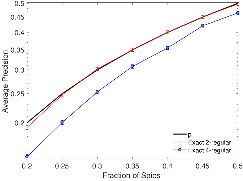
Figure 14. One-to-one transaction forwarding when the adversary knows the graph but does not know the nodes’ internal routing decisions.

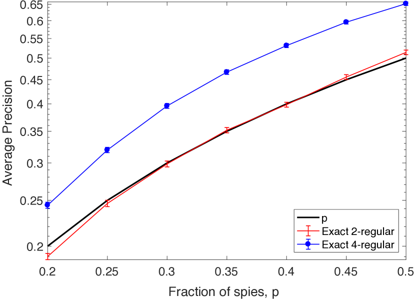
Figure 15. One-to-one transaction forwarding when the adversary knows the graph and knows the nodes’ internal routing decisions.

Appendix C Tradeoffs in graph topology

As discussed in Section 4.2, there are tradeoffs between using 4-regular graphs with one-to-one routing and line graphs (recall that on line graphs, there is only one possible routing scheme, which can be viewed as a special case of one-to-one routing). In this section, we give some more explanation and empirical results detailing these tradeoffs. In our experiments, we have considered three different adversarial settings:

1. An adversary who does not know the underlying graph

2. An adversary who knows the graph, but does not know any routing decisions

3. An adversary who knows the graph and also knows each node’s relay routing decisions. That is, it knows how node $v$ will route incoming transactions from edge $e$, but it does not know how $v$ will route $v$’s own transactions.

Adversarial model (c) is motivated by the fact than an adversary can send probe transactions that get relayed through honest nodes, but it cannot force honest nodes to produce their own transactions. Hence learning a node’s relay routing choices is feasible, whereas learning a node’s own transaction routing choices is significantly more difficult. We also considered two different graph settings:

1. Exact regular graphs (idealized setting)

2. Approximate regular graphs (proposed construction mechanism detailed in Section 4.3)

Since the adversary with no graph knowledge was already discussed in Section 4.1, we focus on adversarial models (b) and (c). We begin by considering an adversary that knows the graph, but not the internal routing decisions. Figure 15 shows the average precision of such an adversary on exact 4-regular and line graphs, each with 100 nodes. The error bars give the standard error for our experiments. Our simulations show that 4-regular graphs have a lower average precision than line graphs. This trend is similar to what we observed for adversaries that do not know the graph, discussed in Section 4.1. However, Figure 15 illustrates the average precision for an adversary that knows both the graph and the internal routing decisions of each node. Here, the trend is reversed: line graphs have a precision that is upper bounded by $p$, whereas on 4-regular graphs, the precision can be higher than $p$. This makes sense because on line graphs, each node has only one possible routing decision, so the additional routing knowledge of the adversary does not help.

These simulated observations suggest that if the adversary is strong enough to learn the internal, random routing decisions of each node, a line graph actually gives greater protections. However, we expect such learning to be expensive, since the only way to learn a node’s routing decisions is to relay transactions through that node. To learn routing decisions for all nodes in the graph will require at least a linear number of transactions in the number of nodes. Such an attack would quickly grow expensive, especially considering that the graph is changing periodically.

References

- (1)
- aws ([n. d.]) [n. d.]. AWS Regions and Endpoints. ([n. d.]). http://docs.aws.amazon.com/general/latest/gr/rande.html.
- bit ([n. d.]) [n. d.]. Bitcoin Core integration/staging tree. ([n. d.]). https://github.com/bitcoin/bitcoin.
- cha ([n. d.]) [n. d.]. Chainalysis. ([n. d.]). https://www.chainalysis.com/.
- kov ([n. d.]) [n. d.]. The Kovri I2P Router Project. ([n. d.]). https://github.com/monero-project/kovri.
- mon ([n. d.]) [n. d.]. Monero. ([n. d.]). https://getmonero.org/home.
- bit (2015) 2015. Bitcoin Core Commit 5400ef6. (2015). https://github.com/bitcoin/bitcoin/commit/5400ef6bcb9d243b2b21697775aa6491115420f3.
- red (2016) 2016. reddit/r/monero. (2016). https://www.reddit.com/r/Monero/comments/4aki0k/what_is_the_status_of_monero_and_i2p/.
- Androulaki et al. (2013) Elli Androulaki, Ghassan O Karame, Marc Roeschlin, Tobias Scherer, and Srdjan Capkun. 2013. Evaluating user privacy in bitcoin. In International Conference on Financial Cryptography and Data Security. Springer, 34–51.
- Apostolaki et al. (2016) Maria Apostolaki, Aviv Zohar, and Laurent Vanbever. 2016. Hijacking Bitcoin: Large-scale Network Attacks on Cryptocurrencies. arXiv preprint arXiv:1605.07524 (2016).
- Athreya and Ney (2004) Krishna B Athreya and Peter E Ney. 2004. Branching processes. Courier Corporation.
- Biryukov et al. (2014) Alex Biryukov, Dmitry Khovratovich, and Ivan Pustogarov. 2014. Deanonymisation of clients in Bitcoin P2P network. In Proceedings of the 2014 ACM SIGSAC Conference on Computer and Communications Security. ACM, 15–29.
- Biryukov and Pustogarov (2015) Alex Biryukov and Ivan Pustogarov. 2015. Bitcoin over Tor isn’t a good idea. In Symposium on Security and Privacy. IEEE, 122–134.
- Bohannon (2016) John Bohannon. 2016. Why criminals can’t hide behind Bitcoin. Science (2016).
- Bojja Venkatakrishnan et al. (2017) Shaileshh Bojja Venkatakrishnan, Giulia Fanti, and Pramod Viswanath. 2017. Dandelion: Redesigning the Bitcoin Network for Anonymity. POMACS 1, 1 (2017), 22.
- Chaum (1988) D. Chaum. 1988. The dining cryptographers problem: Unconditional sender and recipient untraceability. Journal of cryptology 1, 1 (1988).
- Chellappa and Sin (2005) Ramnath K Chellappa and Raymond G Sin. 2005. Personalization versus privacy: An empirical examination of the online consumer’s dilemma. Information technology and management 6, 2 (2005), 181–202.
- Corrigan-Gibbs and Ford (2010) H. Corrigan-Gibbs and B. Ford. 2010. Dissent: accountable anonymous group messaging. In CCS. ACM.
- Danezis et al. (2009) George Danezis, Claudia Diaz, Emilia Käsper, and Carmela Troncoso. 2009. The wisdom of Crowds: attacks and optimal constructions. In European Symposium on Research in Computer Security. Springer, 406–423.
- Danezis et al. (2010) George Danezis, Claudia Diaz, Carmela Troncoso, and Ben Laurie. 2010. Drac: An Architecture for Anonymous Low-Volume Communications.. In Privacy Enhancing Technologies, Vol. 6205. Springer, 202–219.
- Dingledine et al. (2004) R. Dingledine, N. Mathewson, and P. Syverson. 2004. Tor: The second-generation onion router. Technical Report. DTIC Document.
- Fanti et al. (2015) G. Fanti, P. Kairouz, S. Oh, and P. Viswanath. 2015. Spy vs. Spy: Rumor Source Obfuscation. In SIGMETRICS Perform. Eval. Rev., Vol. 43. 271–284. Issue 1.
- Fanti and Viswanath (2017) Giulia Fanti and Pramod Viswanath. 2017. Anonymity Properties of the Bitcoin P2P Network. arXiv preprint arXiv:1703.08761 (2017).
- Freedman and Morris (2002) M.J. Freedman and R. Morris. 2002. Tarzan: A peer-to-peer anonymizing network layer. In Proc. CCS. ACM.
- Frizell (2015) Sam Frizell. 2015. Bitcoins Are Easier To Track Than You Think. Time (January 2015).
- Gencer and Sirer (2017) Adam Efe Gencer and Emin Gün Sirer. 2017. State of the Bitcoin Network. Hacking Distributed, http://hackingdistributed.com/2017/02/15/state-of-the-bitcoin-network/. (February 2017).
- Goel et al. (2003) S. Goel, M. Robson, M. Polte, and E. Sirer. 2003. Herbivore: A scalable and efficient protocol for anonymous communication. Technical Report.
- Golle and Juels (2004) P. Golle and A. Juels. 2004. Dining cryptographers revisited. In Advances in Cryptology-Eurocrypt 2004.
- Heilman et al. (2016) Ethan Heilman, Leen Alshenibr, Foteini Baldimtsi, Alessandra Scafuro, and Sharon Goldberg. 2016. TumbleBit: An untrusted Bitcoin-compatible anonymous payment hub. Technical Report. Cryptology ePrint Archive, Report 2016/575.
- Jedusor (2016) TE Jedusor. 2016. Mimblewimble. (2016).
- Koshy (2013) Philip Koshy. 2013. CoinSeer: A Telescope Into Bitcoin. Ph.D. Dissertation. The Pennsylvania State University.
- Koshy et al. (2014) Philip Koshy, Diana Koshy, and Patrick McDaniel. 2014. An analysis of anonymity in bitcoin using p2p network traffic. In International Conference on Financial Cryptography and Data Security. Springer, 469–485.
- Maxwell (2013) Greg Maxwell. 2013. CoinJoin: Bitcoin privacy for the real world. In Post on Bitcoin Forum.
- McMillen (2017) Dave McMillen. 2017. Mirai IoT Botnet: Mining for Bitcoins? SecurityIntelligence (April 2017).
- Meiklejohn et al. (2013) Sarah Meiklejohn, Marjori Pomarole, Grant Jordan, Kirill Levchenko, Damon McCoy, Geoffrey M Voelker, and Stefan Savage. 2013. A fistful of bitcoins: characterizing payments among men with no names. In Proceedings of the 2013 conference on Internet measurement conference. ACM, 127–140.
- Mezard and Montanari (2009) Marc Mezard and Andrea Montanari. 2009. Information, physics, and computation. Oxford University Press.
- Miller et al. (2015) Andrew Miller, James Litton, Andrew Pachulski, Neal Gupta, Dave Levin, Neil Spring, and Bobby Bhattacharjee. 2015. Discovering Bitcoin’s public topology and influential nodes. (2015).
- Mittal et al. (2013) Prateek Mittal, Matthew Wright, and Nikita Borisov. 2013. Pisces: Anonymous communication using social networks. In NDSS. ACM.
- Nakamoto (2008) Satoshi Nakamoto. 2008. Bitcoin: A peer-to-peer electronic cash system. (2008).
- Ober et al. (2013) Micha Ober, Stefan Katzenbeisser, and Kay Hamacher. 2013. Structure and anonymity of the bitcoin transaction graph. Future internet 5, 2 (2013), 237–250.
- Peterson and Davie (2007) Larry L Peterson and Bruce S Davie. 2007. Computer networks: a systems approach. Elsevier.
- Pinto et al. (2012) P. C. Pinto, P. Thiran, and M. Vetterli. 2012. Locating the source of diffusion in large-scale networks. Physical review letters 109, 6 (2012), 068702.
- Reid and Harrigan (2013) Fergal Reid and Martin Harrigan. 2013. An analysis of anonymity in the bitcoin system. In Security and privacy in social networks. Springer, 197–223.
- Reiter and Rubin (1998) Michael K Reiter and Aviel D Rubin. 1998. Crowds: Anonymity for web transactions. ACM Transactions on Information and System Security (TISSEC) 1, 1 (1998), 66–92.
- Ron and Shamir (2013) Dorit Ron and Adi Shamir. 2013. Quantitative analysis of the full bitcoin transaction graph. In International Conference on Financial Cryptography and Data Security. Springer, 6–24.
- Ruffing et al. (2014) Tim Ruffing, Pedro Moreno-Sanchez, and Aniket Kate. 2014. CoinShuffle: Practical decentralized coin mixing for Bitcoin. In European Symposium on Research in Computer Security. Springer, 345–364.
- Sasson et al. (2014) Eli Ben Sasson, Alessandro Chiesa, Christina Garman, Matthew Green, Ian Miers, Eran Tromer, and Madars Virza. 2014. Zerocash: Decentralized anonymous payments from bitcoin. In Symposium on Security and Privacy. IEEE, 459–474.
- Schrijver (2002) Alexander Schrijver. 2002. Combinatorial optimization: polyhedra and efficiency. Vol. 24. Springer Science & Business Media.
- Sherwood et al. (2005) Rob Sherwood, Bobby Bhattacharjee, and Aravind Srinivasan. 2005. P5: A protocol for scalable anonymous communication. Journal of Computer Security 13, 6 (2005), 839–876.
- van den Hooff et al. ([n. d.]) Jelle van den Hooff, David Lazar, Matei Zaharia, and Nickolai Zeldovich. [n. d.]. Scalable Private Messaging Resistant to Traffic Analysis. ([n. d.]).
- Wang et al. (2014) Zhaoxu Wang, Wenxiang Dong, Wenyi Zhang, and Chee Wei Tan. 2014. Rumor source detection with multiple observations: Fundamental limits and algorithms. In ACM SIGMETRICS Performance Evaluation Review, Vol. 42. ACM, 1–13.
- Wolinsky et al. (2012) David Isaac Wolinsky, Henry Corrigan-Gibbs, Bryan Ford, and Aaron Johnson. 2012. Dissent in Numbers: Making Strong Anonymity Scale.. In OSDI. 179–182.
- Zamani et al. (2013) M. Zamani, J. Saia, M. Movahedi, and J. Khoury. 2013. Towards provably-secure scalable anonymous broadcast. In USENIX FOCI.
- Zantout and Haraty (2011) Bassam Zantout and Ramzi Haraty. 2011. I2P data communication system. In Proceedings of ICN. Citeseer, 401–409.
- Zhu and Ying (2014) Kai Zhu and Lei Ying. 2014. A robust information source estimator with sparse observations. Computational Social Networks 1, 1 (2014), 3.