Large $N$ scaling and factorization in $\mathrm{SU}(N)$ Yang-Mills gauge theory

Abstract

The large $N$ limit of $\mathrm{SU}(N)$ gauge theories is well understood in perturbation theory. Also non-perturbative lattice studies have yielded important positive evidence that ’t Hooft’s predictions are valid. We go far beyond the statistical and systematic precision of previous studies by making use of the Yang-Mills gradient flow and detailed Monte Carlo simulations of $\mathrm{SU}(N)$ pure gauge theories in 4 dimensions. With results for $N=3,4,5,6,8$ we study the limit and the approach to it. We pay particular attention to observables which test the expected factorization in the large $N$ limit. The investigations are carried out both in the continuum limit and at finite lattice spacing. Large $N$ scaling is verified non-perturbatively and with high precision; in particular, factorization is confirmed. For quantities which only probe distances below the typical confinement length scale, the coefficients of the $1/N$ expansion are of $\mathrm{O}(1)$, but we found that large (smoothed) Wilson loops have rather large $\mathrm{O}(1/N^{2})$ corrections. The exact size of such corrections does, of course, also depend on what is kept fixed when the limit is taken.

1 Introduction

An interesting approach to study quantum chromodynamics (QCD) is to consider the order of the gauge group $N$ as a free parameter. As shown by ’t Hooft [1], by taking the large $N$ limit of the perturbative weak coupling expansion, the theory simplifies in many ways, and in fact one can treat theories at finite $N$ as corrections in the “small” parameter $1/N$. Moreover, the large $N$ expansion predicts that quark loop effects are suppressed by a power of $1/N$, so that the weak coupling expansion of large $N$ QCD is dominated by planar diagrams with purely gluonic internal loops. All of these rather remarkable properties of large $N$ QCD, make it an interesting theory to study not only from the theoretical perspective, but also from a practical point of view, as results for real world QCD could be obtained by considering corrections to the $N=\infty$ theory which are parametrized by powers of $1/N$.

Although this $1/N$ scaling is obtained perturbatively, lattice computations provide evidence that it also holds at the non-perturbative level, both in $D=4$ space-time dimensions [2, 3, 4, 5, 6, 7, 8] and in $D=3$ [9, 10, 11, 12, 13]. The evidence is usually based on complicated observables, where typically one needs to project onto ground states by large Euclidean times. It is then difficult to obtain high precision at various $N$ in order to verify ’t Hooft scaling with good confidence. Let us stress the fact that the validity of the $1/N$ scaling, beyond the weak coupling expansion, is not a trivial statement. Hence, it is desirable to test it by means of lattice simulations and with statistically and systematically very precise observables.

Perturbatively, if one carries on with the ’t Hooft $1/N$ topological expansion, another simplification arises, which has to do with the property of factorization

$$\expectationvalue{\mathcal{O}_{1}\mathcal{O}_{2}}=\expectationvalue{\mathcal{O}_{1}}\expectationvalue{\mathcal{O}_{2}}+\mathrm{O}(1/N^{2})\,,$$ (1.1)

where the $\mathcal{O}_{i}$ are local gauge invariant or Wilson loop operators, and the leading correction scales as $1/N^{2}$ in the pure gauge theory, which we focus on for the rest of this work. Eq. (1.1) has several consequences, as it tells us that in the large $N$ limit, the dominant part of a correlator is the disconnected one. In particular, when $\mathcal{O}_{1}=\mathcal{O}_{2}$, this means that fluctuations are suppressed; and as discussed in LABEL:\cite[cite]{[\@@bibref{}{missing}{}{}]}Yaffe:1981vf, this fact can be put in analogy with the classical limit of a quantum theory, where $1/N$ plays the role of $\hbar$. Related to this is also the concept of the “master field”, i.e., the idea that the path integral is dominated by a single gauge configuration (or rather a gauge orbit) [15, 16]. Although these ideas triggered hope to find the solution of large $N$ QCD, such an analytical solution is still lacking today. The situation in the Yang-Mills theories is similar in this respect to two-dimensional $\mathrm{SU}(N)$$\times$$\mathrm{SU}(N)$ spin models[17], while for O$(N)$ models and CP$(N)$ models the large $N$ limit is solvable and one can therefore really carry out the expansion [18, 19, 20].

One more aspect where Eq. (1.1) plays a crucial role has to do with the idea of volume independence, which starting from the work of the authors in LABEL:\cite[cite]{[\@@bibref{}{missing}{}{}]}Eguchi:1982nm, has been used in the lattice formulation to study the large $N$ limit of the Yang-Mills theory by performing simulations in small spacetime volumes [22], and even in single site lattices, provided a clever choice of boundary conditions [23, 24, 25] is made. Clearly, the possibility to compute observables on a single site lattice makes simulations of $\mathrm{SU}(N)$ Yang-Mills theory at large $N$ more accessible, as there is a significant compensation of the extra cost for increasing $N$ by the much smaller number of lattice sites.

The above indicates that factorization is not only relevant in the theoretical context, but also on the practical level, as it is a requirement for the single site lattice simulations to be valid. To be more precise, the equivalence between the single site and the infinite volume theory is argued for on the basis of the Makenko-Migdal loop equations [26] on the lattice. As originally shown in LABEL:\cite[cite]{[\@@bibref{}{missing}{}{}]}Eguchi:1982nm, the loop equations in both theories are equivalent, provided that the product of the expectation value of the Wilson loops factorize as stated in Eq. (1.1). Additionally, we would like to point out that important physics is contained in the corrections to factorization. The most obvious one is that glueball masses are obtained from the connected correlation functions of Wilson loops.

The previous discussion motivates the search for a non-perturbative proof, beyond the realm of weak coupling perturbation theory. Several authors have investigated factorization beyond perturbation theory [27, 28, 29, 30], but no verification has been carried through using the non-perturbative framework provided by numerical simulations of lattice gauge theories. We here fill this gap. In addition, the observables that we consider make it possible to study the large $N$ scaling up to very high precision, and hence address the important issue of the size of the corrections to $N=\infty$.

This paper is organized as follows, in Sec. 2 we present the observables that are used both to check the large $N$ scaling, as well as factorization. In Sec. 3 we discuss different ways of defining the large $N$ limit and in particular the two choices we made for our investigation. In Sec. 4 we describe the ensembles and lattice parameters used for the simulations and in Sec. 5 we present our results, both at finite lattice spacing, and in the continuum limit. We finish with a short summary of the results.

2 Observables

The basic observables we consider are the Yang-Mills action density $E(t)$ at positive flow time [31] (defined below) and rectangular Wilson loop operators

$$W_{C}=\frac{1}{N}\tr P\left\{\exp\left(\oint_{C}A_{\mu}(x)\,\mathrm{d}x^{\mu}\right)\right\}\,,$$ (2.2)

where $C$ is a closed rectangular path in space-time, and $P$ denotes the path ordering operator. The normalization factor $1/N$ is included in the definition of $W_{C}$ in order to have a finite large $N$ limit — already at tree-level. Wilson loops have singularities which have to be removed before the continuum limit can be taken. In particular, for our square Wilson loops, one must remove not just the “perimeter” divergences but also “corner” divergences [32, 33, 34]. One way to proceed is to consider Creutz ratios [35], which however, for loops of large size in lattice units, suffer from small signal to noise ratios. As this would compromise our desire for a precision test, we work instead with smooth Wilson loops. The smoothing is provided by the Yang-Mills gradient flow [36, 37]. It evolves the gauge fields $A_{\mu}(x)$ according to the flow equation

$$\partial_{t}B_{\mu}(t,x) =D_{\nu}G_{\nu\mu}(t,x)\,,\quad B_{\mu}(0,x)=A_{\mu}(x)\,$$ (2.3)

$$G_{\mu\nu}(t,x) =\partial_{\mu}B_{\nu}(t,x)-\partial_{\nu}B_{\mu}(t,x)-\left[B_{\mu}(t,x),B_{\nu}(t,x)\right]\,,$$

where the dimension two parameter $t$ is known as the flow time. The loops at positive flow time are then simply

$$W_{C}(t)=\frac{1}{N}\tr P\left\{\exp\left(\oint_{C}B_{\mu}(t,x)\,\mathrm{d}x^{\mu}\right)\right\}\,.$$ (2.4)

Choosing $8t$ to be of a typical QCD size, say of the order of the square of the inverse string tension, they benefit from small statistical errors even for large loops [38]. In particular, their variance remains finite in the continuum limit. That property is a particular manifestation of the most important feature of observables which are built from the smoothed gauge fields $B_{\mu}(t,x)$: they are renormalized operators at positive flow time $t$ [31, 39]. In other words, there is no renormalization scheme or scale dependence beyond $t$ and the continuum limit is unambiguous and well defined. Even the action density

$$E(x)=-\frac{1}{2}\tr\left\{G_{\mu\nu}(x)G_{\mu\nu}(x)\right\}\,,$$ (2.5)

is finite. It will be one of our observables.

2.1 The gradient flow coupling at large $N$

The gradient flow can also be used to define a renormalized coupling [37]. Using the perturbative expansion of the Yang-Mills energy density at positive flow time $\expectationvalue{E(t)}$, one has that

$$\bar{\lambda}_{\mathrm{GF}}(\mu)=\frac{128\pi^{2}}{3}\left(\frac{N}{N^{2}-1}\right)t^{2}\expectationvalue{E(t)}\Big{\rvert}_{\mu=1/\sqrt{8t}}=\bar{\lambda}_{\overline{\mathrm{MS}}}(\mu)\left[1+c_{1}\bar{\lambda}_{\overline{\mathrm{MS}}}(\mu)+\cdots\right]\,,$$ (2.6)

where $\bar{\lambda}_{\overline{\mathrm{MS}}}(\mu)=N\bar{g}^{2}_{\overline{\mathrm{MS}}}(\mu)$ is the ’t Hooft coupling at the scale $\mu=1/\sqrt{8t}$ and $c_{1}=\frac{1}{16\pi^{2}}\left(\frac{11}{3}\gamma_{E}+\frac{52}{9}-3\ln 3\right)$ is $N$ independent. With this definition, we can then define a scale by setting the renormalized coupling $\bar{\lambda}_{\mathrm{GF}}$ to a given value. A convenient choice for $\mathrm{SU}(3)$ is the reference scale $t_{0}$ [37], which corresponds to a value of the coupling such that $t^{2}\expectationvalue{E(t)}|_{t=t_{0}}=0.3$. This particular choice can be generalized to $\mathrm{SU}(N)$ if the right hand side is modified so that it has the correct scaling with $N$. Clearly, we also want the definition to remain what it is for $N=3$. Thus, Eq. (2.6), suggests to define $t_{0}$ implicitly by the equation [2]

$$t^{2}\expectationvalue{E(t)}\rvert_{t=t_{0}}=0.1125\,\frac{N^{2}-1}{N}\,,$$ (2.7)

for all $N$.

2.2 Smooth Wilson loops

The favourable properties of smooth Wilson loops have already been exploited in the literature, as for example to estimate the string tension at small values of $t$ in Refs. [6, 39], or to study the large $N$ phase transition in the eigenvalue spectrum of the Wilson loop matrices [40]. For our purpose, the limit of small $t$ is not required, as the smooth loops are used to test factorization and the large $N$ limit for well defined renormalized observables, regardless of their relation to the operators at $t=0$.

In the end, we study the large $N$ limit of square Wilson loops, i.e. for loops where the path $C$ in Eq. (2.4) is given by a square of size $R\times R$. In order to take the large $N$ limit, the loops are matched at different $N$ relating their size to the scale $t_{0}$ introduced in the previous section. More precisely, the large $N$ and continuum limits are taken for loops of size $R_{c}=\sqrt{8ct_{0}}$ (see Figure 1), where the smoothing parameter $t=ct_{0}$, and $c$ is a constant parameter.

To be more precise, let us denote a square loop with one of its corners at the spacetime point $(x_{0},\vec{x})$ and extending only in space as $W(t,x_{0},\vec{x},R)$. Its expectation value

$$W(c)=\left\langle W(t,x_{0},\vec{x},R_{c})\right\rangle\,\quad\text{with }\quad t=ct_{0}\,,R_{c}=\sqrt{8ct_{0}}\,,\;$$ (2.8)

is independent of the position $\vec{x}$ due to translation invariance and only depends on the parameter $c$. In our notation we separate time and space-coordinates, as we will later use lattices with different boundary conditions in time (open b.c.) and space (periodic b.c.). While the independence on $\vec{x}$ is exact, $x_{0}$ has to be sufficiently far away from the boundary for Eq. (2.8) to hold.

Similarly, we define

$$W^{\mathrm{sq}}(c)=\left\langle W^{2}(t,x_{0},\vec{x},R_{c})\right\rangle\,\quad\text{with }\quad t=ct_{0}\,,R_{c}=\sqrt{8ct_{0}}\,,\;$$ (2.9)

which corresponds to the expectation value of the product of a Wilson loop with itself.

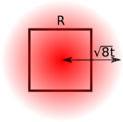
Figure 1: Schematic representation of a smooth Wilson loop operator. The size of the loop is chosen such that it has the same length as the smoothing radius, i.e. $R=\sqrt{8t}$.

2.3 Observables to test factorization

In order to investigate the property of factorization from Eq. (1.1), we define several observables based on the Yang-Mills action density and the smooth Wilson loops at positive flow time. They are constructed such that factorization implies that they vanish as $N\to\infty$. First we consider the simplest case of the observable $G_{W}$ defined in terms of the smooth Wilson loops as

$$G_{W}(c)=\frac{W^{\mathrm{sq}}(c)-W^{2}(c)}{W^{2}(c)}\,.$$ (2.10)

Then, we consider observables built from the space integral of the smooth Wilson loops and the Yang-Mills action density. We define

$$H_{\mathcal{O}}(c)=\left(\frac{1}{t_{0}^{3/2}}\right)\frac{{\bigint}\mathrm{d}^{3}\vec{x}\,\left[\expectationvalue{\mathcal{O}(ct_{0},x_{0},\vec{x})\mathcal{O}(ct_{0},x_{0},\vec{0})}-\expectationvalue{\mathcal{O}(ct_{0},x_{0},\vec{x})}^{2}\right]}{\expectationvalue{\mathcal{O}(ct_{0},0,\vec{x})}^{2}}\,,$$ (2.11)

with the factor $1/t_{0}^{3/2}$ rendering $H_{\mathcal{O}}(c)$ dimensionless, and where $\mathcal{O}$ is either a smooth Wilson loop, or the Yang-Mills action density. Notice that $H$ is a type of susceptibility, as we are integrating over the contributions from the correlation function of $\mathcal{O}$ at different distances. The integration does not extend over $x_{0}$ due to our choice of boundary conditions and $x_{0}$ is again supposed to be far away from the time-boundaries. In comparison to the simple observable $G_{W}$, this probes longer distances, but introduces also more noise and affects the statistical errors in the measurements. Nonetheless, as will be shown in Sec. 5, the statistical precision that can be achieved for $H_{\mathcal{O}}$ remains good. In particular, we will consider $H_{E}(c)$, defined by inserting

$$\mathcal{O}(t,x_{0},\vec{x})=E(t,x_{0},\vec{x})\,,$$ (2.12)

into Eq. (2.11) and $H_{W}$ by

$$\mathcal{O}(t,x_{0},\vec{x})=W(t,x_{0},\vec{x},R_{c})\,.$$ (2.13)

We remind the reader of our choice $R_{c}=\sqrt{8ct_{0}}$.

Eq. (1.1) means

$$H_{E}\raisebox{-0.43057pt}{ $\stackrel{{\scriptstyle\small{N\to\infty}}}{{\sim}}$}\,1/N^{2}\,,\;\;G_{W}\raisebox{-0.43057pt}{ $\stackrel{{\scriptstyle\small{N\to\infty}}}{{\sim}}$}\,1/N^{2}\,,\;\;H_{W}\raisebox{-0.43057pt}{ $\stackrel{{\scriptstyle\small{N\to\infty}}}{{\sim}}$}\,1/N^{2}\,.$$ (2.14)

2.4 Finite volume

For a numerical test, we need to choose a finite volume. We chose our parameters such that $L/\sqrt{8t_{0}}\approx 3.3$. Table 1 shows the actual values used in our simulations. Since $L$ is thus approximately constant, it is omitted as an argument of the observables. We note that the large $N$ limit and factorization can be tested in infinite or in finite volume. To be on the safe side, we chose the latter, even though we are not far from the infinite volume limit for most observables.

3 Defining the approach to the large $N$ limit

The complete definition of a quantum field theory involves a regularization (here Wilson’s lattice theory) as well as a non-trivial renormalisation before the regulator can be removed. Although this is usually not discussed, quantitative statements about the approach to the large $N$ limit, such as the ones we are seeking here, do depend on the renormalisation scheme if the renormalisation scheme defines which quantity is held fixed as we take $N\to\infty$.

While the $\mathrm{O}(1/N^{2})$ corrections depend on these details, the true limit is expected to be unique in the following sense. It is independent of the scheme, as long as the ’t Hooft coupling $\bar{\lambda}_{s}(\mu)=N\bar{g}^{2}_{s}(\mu)$ in any scheme is kept fixed as one takes the limit. This statement becomes most transparent when we replace couplings by the associated $\Lambda$-parameters,

$$\Lambda_{s}\,=\lim_{\mu\to\infty}\,\mu\,\left(\frac{48\pi^{2}}{11\lambda_{s}(\mu)}\right)^{51/121}\exp\left(-\frac{1}{b_{0}\lambda_{s}(\mu)}\right)\,,\quad b_{0}=\frac{11}{24\pi^{2}}\,.$$ (3.15)

Now any renormalization group invariant quantity $\mathcal{O}$ of mass dimension $n$, has a large $N$ limit

$$\lim_{N\to\infty}\frac{\mathcal{O}}{\Lambda_{s}^{n}}=\lim_{N\to\infty}r^{n}(N)\frac{\mathcal{O}}{\Lambda_{s^{\prime}}^{n}}=r_{\infty}^{n}\,\lim_{N\to\infty}\frac{\mathcal{O}}{\Lambda_{s^{\prime}}^{n}}\,,$$ (3.16)

where

$$r(N) = \exp(c_{ss^{\prime}}(N)/b_{0})\,,$$ (3.17)

$$\lambda_{s^{\prime}} = \lambda_{s}+c_{ss^{\prime}}(N)\lambda_{s}^{2}+\mathrm{O}(\lambda_{s}^{3})\,.$$ (3.18)

and

$$r_{\infty}=\exp(\lim_{N\to\infty}c_{ss^{\prime}}(N)/b_{0})\,.$$ (3.19)

Examples for $n=1$ are glueball masses and $t_{0}$ defined above is a RGI scale with $n=-2$. When the observable $\mathcal{O}$ depends on external momenta or coordinates, they have to be fixed in units of $\Lambda$ in a specified scheme, e.g. $\Lambda_{\overline{\mathrm{MS}}}$, when taking $N\to\infty$.

Due to the existence of the limit eq. (3.16), we may also scale distances with respect to any one particular reference scale (choice of $\mathcal{O}$). In our numerical work we have chosen $t_{0}$, eq. (2.7), because of its high precision.

The preceding discussion is about the continuum theory. It thus saliently assumes that first we take the continuum limit at finite $N$ and then we perform $N\to\infty$. However, we may also proceed in the opposite order: first take the large $N$ limit at fixed lattice spacing and then send the lattice spacing to zero. Let us briefly discuss that this order of limits is indeed the same as above; the limits are interchangeable.

3.1 Large $N$ limit at fixed lattice spacing

The existence of the large $N$ limit at fixed finite lattice spacing is expected due to the following consideration. We start from the Lambda-parameter, $\Lambda_{\mathrm{lat}}$ in the lattice minimal subtraction scheme, which satisfies eq. (3.15) with $\mu=1/a$ and $\lambda_{\mathrm{lat}}(\mu)=\lambda_{0}$ in terms of the lattice spacing, $a$, and the bare coupling, $\lambda_{0}=Ng_{0}^{2}$. In fact, having a specific scheme, the lat-scheme, we can give the more detailed formula,

$$a\Lambda_{\mathrm{lat}}\,=\,\,\left(\frac{48\pi^{2}}{11\lambda_{0}}\right)^{51/121}\exp\left(-\frac{24\pi^{2}}{11\lambda_{0}}\right)\left(1+c_{1}(N)\lambda_{0}+\mathrm{O}(\lambda_{0}^{2})\right)\,,$$ (3.20)

where $c_{1}=0.1048+\mathrm{O}(1/N^{2})$ [41]. Eq. (3.20) shows that the large $N$ limit can be taken at fixed bare coupling which is equivalent to fixed lattice spacing $a$. Apart from $\mathrm{O}(1/N^{2})$ terms in $c_{1}$ and higher order terms, fixed lattice spacing is the same as fixed $\Lambda_{\mathrm{lat}}$ and therefore also fixed $\Lambda_{s}$ in other schemes. See also an early discussion of $\Lambda_{\overline{\mathrm{MS}}}/\Lambda_{\mathrm{lat}}$ including its $N$ dependence [42].

In general, taking the large $N$ limit at fixed lattice spacing has to be followed by the $a\to 0$ limit at $N=\infty$. However, when we investigate factorization, the second step is not expected to be necessary. This is because the perturbative proof of factorization holds in the lattice regularization [43] at finite $a$. If factorization holds non-perturbatively we thus also expect eq. (2.14) at any fixed $a$. In any case, verifying eq. (2.14) at arbitrary finite lattice spacing implies that it holds in the continuum limit.

Note also that even the large $N$ limit of divergent quantities, such as Wilson loops at $t=0$, is expected to exist. A high precision numerical test has recently been performed [8].

4 Lattice details

In this section we give the details of our lattice simulations. We simulate the pure gauge theory with $N=3,\,4,\,5,\,6,\,8$ at several lattice spacings. The lattice action is the Wilson gauge action and we use open boundary conditions in the time direction [44]. The simulations are performed using a combination of heatbath and overrelaxation local updates using the Cabibbo-Marinari strategy [45] to refresh the $\mathrm{SU}(N)$ matrices. The ratio of overrelaxation to heatbath updates is fixed to $L/(2a)$.

For convenience, we present the values of the lattice spacing, as well as lattice sizes in physical units by assigning a value to $t_{0}$ such that $\sqrt{t_{0}}=0.166\,\mathrm{fm}$. This choice is motivated by the result in $\mathrm{SU}(3)$ for $\sqrt{8t_{0}}/r_{0}=0.941(7)$ [46] and the value of the reference scale $r_{0}\approx 0.5\,\mathrm{fm}$ [47]. Notice that this choice is somewhat arbitrary, as apart from the missing quark loops, for $N\neq 3$ the theory cannot be directly identified with Nature.

The parameters of the simulations are displayed in Table 1. The configurations used for the measurements are a subset of those reported in LABEL:\cite[cite]{[\@@bibref{}{missing}{}{}]}Ce:2016awn for all ensembles except for those at $N=3,8$, and for the finest lattice spacings in the case of $N=4,5$. As announced above, all the lattices considered in Table 1 are of approximately the same spatial size $L\approx 1.55\,\mathrm{fm}$. In addition, we have used two additional ensembles with $L\approx 2.35\,\mathrm{fm}$ at the coarsest lattice spacing ($a\approx 0.1\,\mathrm{fm}$) for $N=4,5$ in order to check for effects due to small variations in the volume. Notice that for the ensembles which have been reported in LABEL:\cite[cite]{[\@@bibref{}{missing}{}{}]}Ce:2016awn, we have a very large number of measurements for the Yang-Mills action density.

#run	$N$	$\beta$	$T/a$	$L/a$	$a[\mathrm{fm}]$	$N_{\mathrm{meas}}^{\mathrm{W}}$	$N_{\mathrm{meas}}^{\mathrm{E}}$	$t_{0}/a^{2}$	$L/\sqrt{8t_{0}}$
$A(3)_{2}$	3	6.11	80	20	0.078	320	6720	$4.5776(15)^{*}$	3.3050(5)
$A(3)_{3}$	3	6.24	96	24	0.064	280	280	$6.783(23)$	3.258(6)
$A(3)_{4}$	3	6.42	96	32	0.050	252	252	$11.19(4)$	3.382(6)
$A(4)_{1}$	4	10.92	64	16	0.096	248	17341	$2.9900(7)^{**}$	3.2714(4)
$A(4)_{2}$	4	11.14	80	20	0.078	300	35960	$4.5207(8)^{**}$	3.3257(3)
$A(4)_{3}$	4	11.35	96	24	0.065	312	15460	$6.4849(16)^{**}$	3.3321(4)
$A(4)_{4}$	4	11.65	96	32	0.049	320	640	$11.55(3)$	3.329(4)
$A(5)_{1}$	5	17.32	64	16	0.095	320	9871	$3.0636(7)^{**}$	3.2319(4)
$A(5)_{2}$	5	17.67	80	20	0.077	240	21680	$4.6751(8)^{**}$	3.2703(3)
$A(5)_{3}$	5	18.01	96	24	0.064	248	8007	$6.8151(18)^{**}$	3.2504(4)
$A(5)_{4}$	5	18.21	96	32	0.049	328	328	$11.51(3)$	3.334(4)
$A(6)_{1}$	6	25.15	64	16	0.095	320	19360	$3.0824(4)^{**}$	3.2220(2)
$A(6)_{2}$	6	25.68	80	20	0.076	264	11392	$4.8239(9)^{**}$	3.2195(3)
$A(6)_{3}$	6	26.15	96	24	0.063	288	6704	$6.9463(13)^{**}$	3.2195(3)
$A(8)_{2}$	8	32.54	20	80	0.076	320	320	$4.782(5)$	3.2336(17)

Table 1: Parameters of the simulations. For each of the gauge groups $\mathrm{SU}(N)$ we give the inverse lattice coupling $\beta=2N^{2}/\lambda_{0}$, the dimensions of the lattice, the approximate lattice spacing using $\sqrt{t_{0}}=0.166\,\mathrm{fm}$ followed by the number $N_{\mathrm{meas}}^{\mathrm{W}}$ of measurements used for the computation of the smooth Wilson loops, and $N_{\mathrm{meas}}^{\mathrm{E}}$ for the action density, eq. (2.5). In the second to last column we present the values of $t_{0}/a^{2}$:$~{}^{*}$ taken from LABEL:\cite[cite]{[\@@bibref{}{missing}{}{}]}Vera:2016xpp and$~{}^{**}$ taken from LABEL:\cite[cite]{[\@@bibref{}{missing}{}{}]}Ce:2016awn.

The flow equations are integrated using a third order Runge-Kutta integrator [37] and the observables are measured at intervals $\Delta t$ of $t$ of $\Delta t/a^{2}\approx 2-3\times 10^{-2}$. Afterwards, they are interpolated using a second order polynomial in order to obtain their values at arbitrary $t$. The action density is defined exactly as in [37], using the clover discretization and it is measured from $t=0$ up to $t\approx 1.2\,t_{0}$. The loops, $W(c)$, are measured only in the vicinity of $t=ct_{0}$, with $c={1/2,1,9/4}$, and then interpolated to the exact value of $t$. For the loops, one has to do an additional interpolation to $R_{c}$, and since their statistical precision is very high, one has to be careful with small potential systematic effects. The details of this interpolation were already presented in LABEL:\cite[cite]{[\@@bibref{}{missing}{}{}]}Vera:2017dxr.

We end this section with the precise definition of the observables introduced in Eqs. (2.8)-(2.11) on the lattice. First, for the Wilson loops we use translation invariance in the form

$$W(c) =\frac{a^{4}}{\left(T-2d\right)L^{3}}\sum_{x_{0}=d}^{T-d-a}\sum_{\vec{x}}\expectationvalue{W(ct_{0},x_{0},\vec{x},R_{c})}\,,$$

$$W^{\mathrm{sq}}(c) =\frac{a^{4}}{\left(T-2d\right)L^{3}}\sum_{x_{0}=d}^{T-d-a}\sum_{\vec{x}}\expectationvalue{W(ct_{0},x_{0},\vec{x},R_{c})^{2}}\,,$$ (4.21)

where $\expectationvalue{\cdot}$ corresponds to the estimator of the true expectation value computed on the lattice.

In order to compute $H_{W}$, we define

$$W^{\mathrm{sq}}_{\mathrm{int}}(c)=\frac{a}{(T-2d)}\sum_{x_{0}=d}^{T-d-a}\expectationvalue{\left(\frac{a^{3}}{L^{3}}\sum_{\vec{x}}W(ct_{0},x_{0},\vec{x},R_{c})\right)^{2}}\,,$$ (4.22)

so that

$$H_{W}(c)=\left(\frac{L^{3}}{t_{0}^{3/2}}\right)\frac{W^{\mathrm{sq}}_{\mathrm{int}}(c)-W^{2}(c)}{W^{2}(c)}\,,$$ (4.23)

and we proceed in a similar way to define $H_{E}$ after replacing $W(ct_{0},x_{0},\vec{x},R_{c})$ by $t^{2}E(ct_{0},x_{0},\vec{x})\rvert_{t=ct_{0}}$. The parameter $d$ is introduced to deal with the systematic effects from the open boundary conditions. It is chosen in a similar way as described in LABEL:\cite[cite]{[\@@bibref{}{missing}{}{}]}Ce:2016uwy, so that the effects coming from the boundaries are negligible with respect to the statistical error in the bulk.

5 Results

5.1 Large $N$ scaling

In order to test and provide a precise verification of $1/N^{2}$ scaling, we analyse our results for $W(c)$ and for the gradient flow coupling $\bar{\lambda}_{\mathrm{GF}}$. Let us first discuss our results for the latter.

5.1.1 The gradient flow coupling

In Figure 2 we plot $\bar{\lambda}_{\mathrm{GF}}$ as a function of $t$ for several gauge groups and different lattice spacings. Within the scale of the plot, the results are hard to distinguish for all gauge groups, which already shows the small size of the $N$ dependent corrections. While at $t=t_{0}$ indepencence of $N$ is enforced by Eq. 2.6 or equivalently

$$\bar{\lambda}_{\mathrm{GF}}(1/\sqrt{8t_{0}})=0.3\times 16\pi^{2}\,,$$ (5.24)

the different $N$ curves remain remarkably close when $t$ is a factor of 5 away from $t_{0}$. At a closer look, corrections to $N=\infty$ are present and the data agrees very well with a polynomial in $1/N^{2}$ as expected. We verified this by interpolating the data to several values of $t$ in a regular interval from $t=0.1\,t_{0}$ to $t=1.1\,t_{0}$, and then taking the large $N$ limit once at a fixed lattice spacing and once in the continuum.

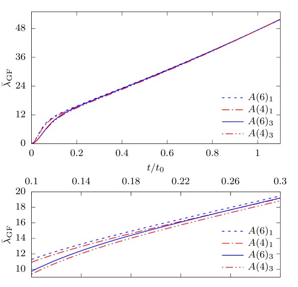
Figure 2: $\bar{\lambda}_{\mathrm{GF}}$ as a function of $t$ for several values of $N$ and $a$ (see Table 1). In the lower plot, we present a closer look at the small $t$ region.

As can be observed in Figure 2, cut-off effects are large at small $t$. At $t=0.1\,t_{0}$ the relative difference between the results at the finest lattice spacing ($a\approx 0.05\,\mathrm{fm}$) and at the coarsest ($a\approx 0.1\,\mathrm{fm}$) one, is around $20\%$; while the errors in the measurements themselves is at the per-mill level. The situation is better at larger values of $t$, so let us first focus on values of $t/t_{0}\geq 0.3$, where the relative size of cut-off effects is reduced tenfold, when compared to the case at $t/t_{0}=0.1$. In Figure 3 we show a plot of the continuum extrapolation of $\bar{\lambda}_{\mathrm{GF}}$ at $t/t_{0}=0.8$ and the large $N$ extrapolation both at finite lattice spacing and in the continuum. In order to be able to use the dataset at $N=8$, in addition to the continuum limit extrapolations, we consider $a^{2}/t_{0}=0.2091$, the value on ensemble A(8)₂. We then interpolated the results for all the other gauge groups to that lattice resolution.

On the left panel of Figure 3 we show the continuum limit extrapolations. The strategy chosen for the extrapolation is the following: all continuum extrapolations are performed by linear fits in $a^{2}/t_{0}$ to those data which satisfy $a^{2}/t_{0}\leq 1/4$ (default fit). Such a restriction has been well motivated in LABEL:\cite[cite]{[\@@bibref{}{missing}{}{}]}DallaBrida:2016kgh for $N=3$ and we find smaller discretization effects for larger $N$. As an estimate of the systematic uncertainty associated with this choice, we perform a second fit linear in $a^{2}$ with a data point at larger $a^{2}$; if the latter fit does not have a good $\chi^{2}$ we add an $a^{4}/t^{2}$ term to the fit-function (control fit). If necessary, the error of the default fit is enlarged until it covers the full 1-$\sigma$ band of the control fit. The uncertainties of the continuum limit points are usually dominated by the systematics which arises from different fits and which is not necessarily independent for different $N$.

All values of $\chi^{2}/\mathrm{dof}$ are excellent except for $\mathrm{SU}(4)$, where we obtain a value of $2.2$ and $2.7$ for the linear and quadratic fits respectively. After performing the fits in $a^{2}/t_{0}$, on the right panel of Figure 3 we plot the large $N$ extrapolations both in the continuum and at finite lattice spacing. As discussed, $N=8$ is available only at finite lattice spacing, where in addition, errors are much smaller due to the fact that we performed an interpolation instead of the continuum limit extrapolation. The large $N$ extrapolation uses the form

$$Y(1/N^{2})=a_{0}\left(1+\frac{a_{1}}{N^{2}}+\frac{a_{2}}{N^{4}}\right)\,.$$ (5.25)

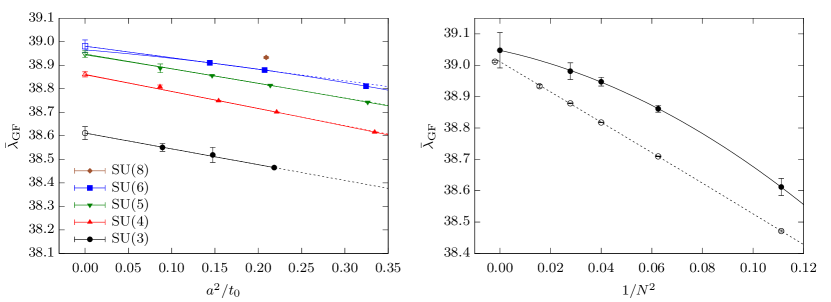
Figure 3: Left: Continuum extrapolation of $\bar{\lambda}_{\mathrm{GF}}$ at $t/t_{0}=0.8$ for all the different gauge groups. Right: Large $N$ extrapolations of $\bar{\lambda}_{\mathrm{GF}}$ in the continuum limit (solid line) and at finite lattice spacing, $a^{2}/t_{0}=0.2091$, (dotted line). The points at finite lattice spacing have been slightly shifted for better legibility.

As seen in Figure 3, the fit to the function $Y$ is excellent, with a $\chi^{2}/\mathrm{dof}=1.02$ at finite lattice spacing; for the continuum points we do not consider $\chi^{2}$ since the errors are strongly correlated due to the dominating systematic uncertainty of the continuum extrapolations. Notice also that the results suggest that cut-off effects decrease with increasing $N$.

As an example of results at smaller $t$, we show our analysis at $t/t_{0}=0.4$ in Figure 4. In this case, the magnitude of the cut-off effects is larger, but the same analysis as before can be carried out.

As mentioned earlier, dealing with $\bar{\lambda}_{\mathrm{GF}}$ at values of $t/t_{0}\leq 0.3$ presents a bigger challenge, so one cannot reach the same level of accuracy as the results presented in this section. However, we have proceeded to do a similar analysis for such small values of $t$, including corrections of higher order in $a^{2}/t_{0}$. Details are found in Appendix B.

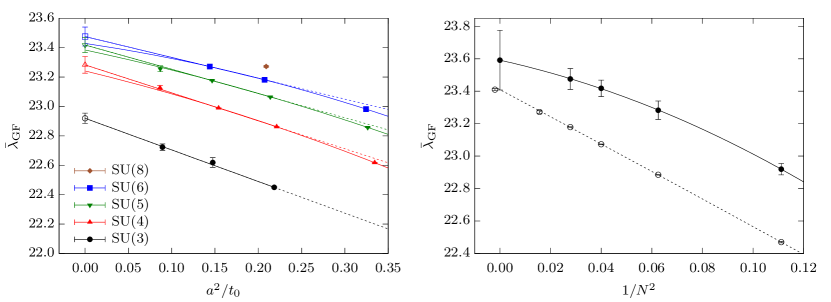
Figure 4: Left: Continuum extrapolation of $\bar{\lambda}_{\mathrm{GF}}$ at $t/t_{0}=0.4$ for all the different gauge groups. Right: Large $N$ extrapolations of $\bar{\lambda}_{\mathrm{GF}}$ in the continuum (solid line) and at finite lattice spacing (dotted line). The points at finite lattice spacing have been slightly shifted for better legibility.

From the above analysis, we find that the large $N$ dependence of $\bar{\lambda}_{\mathrm{GF}}$ is in excellent agreement with the $1/N^{2}$ scaling predicted by the ’t Hooft perturbative expansion. Moreover, defining

$$\eta(1/N^{2})=\Big{\lvert}\frac{Y(0)-Y(1/N^{2})}{Y(0)}\Big{\rvert}\,,$$ (5.26)

we can determine the “distance” between $\mathrm{SU}(3)$ and $\mathrm{SU}(\infty)$. In the continuum, at $t/t_{0}=0.8$ and $t/t_{0}=0.4$ we find $\eta(1/9)=1.1\%$ and $2.8\%$ respectively. Note also that the large $N$ limit is taken at fixed $t_{0}$ and therefore $\eta\equiv 0$ at $t=t_{0}$ by definition. To account for this effect, we also fit $Y$ to $\bar{\lambda}_{\mathrm{GF}}(1/\sqrt{8t})-\bar{\lambda}_{\mathrm{GF}}(1/\sqrt{8t_{0}})$ instead of $\bar{\lambda}_{\mathrm{GF}}(1/\sqrt{8t})$, and define $\delta$ in a similar way to $\eta$. The results, together with those obtained for $\eta$ are displayed in Table 2. Let us remark that the individual errors in our measurements are below the per-mill level, so we can confidently quantify these percent level deviations between $\mathrm{SU}(3)$ and $\mathrm{SU}(\infty)$.

The magnitude of the $1/N^{2}$ corrections can be read off from the coefficients $a_{1}$ and $a_{2}$ collected in Table 2, together with those of the smooth Wilson loops which we discuss next.

obs.	$c$	fit	$a_{0}$	$a_{1}$	$a_{2}$	$\chi^{2}/\mathrm{dof}$	$\eta(1/9)$	$\delta(1/9)$
$\bar{\lambda}_{\mathrm{GF}}$	$0.2$	L	$15.916(6)$	$-0.472(15)$	$-0.05(12)$	$0.79$	$0.05$	$0.03$
$\bar{\lambda}_{\mathrm{GF}}$	$0.4$	L	$23.410(6)$	$-0.3567(90)$	$-0.043(70)$	$1.07$	$0.04$	$0.04$
$\bar{\lambda}_{\mathrm{GF}}$	$0.8$	L	$39.011(3)$	$-0.1233(30)$	$-0.011(25)$	$1.02$	$0.014$	$0.06$
$\bar{\lambda}_{\mathrm{GF}}$	$0.2$	C	$16.2(5)$	$-0.08(96)$	$-1.9(65)$	$0.44$	$0.03$	$0.02$
$\bar{\lambda}_{\mathrm{GF}}$	$0.4$	C	$23.6(2)$	$-0.15(26)$	$-1.0(18)$	$0.01$	$0.03$	$0.03$
$\bar{\lambda}_{\mathrm{GF}}$	$0.8$	C	$39.05(6)$	$-0.045(45)$	$-0.50(32)$	$0.02$	$0.011$	$0.05$
$W$	$1/2$	L	$0.7760(7)$	$0.355(33)$	$-0.09(24)$	$0.49$	$0.04$	$-$
$W$	$1$	L	$0.6575(3)$	$0.449(22)$	$0.66(22)$	$0.49$	$0.06$	$-$
$W$	$9/4$	L	$0.4228(7)$	$0.626(85)$	$2.67(82)$	$0.51$	$0.10$	$-$
$W$	$1/2$	C	$0.792(4)$	$0.17(19)$	$0.8(13)$	$0.11$	$0.03$	$-$
$W$	$1$	C	$0.666(3)$	$0.54(14)$	$-0.5(10)$	$0.01$	$0.05$	$-$
$W$	$9/4$	C	$0.426(9)$	$1.27(69)$	$-3.4(46)$	$0.24$	$0.10$	$-$

Table 2: Parameters of the large $N$ extrapolations, eq. (5.25), of $\bar{\lambda}_{\mathrm{GF}}(1/\sqrt{8ct_{0}})$ and $W(c)$ at finite lattice spacing (L) and in the continuum (C).

5.1.2 Smooth Wilson loops

We have determined the smooth Wilson loops at three different values of $c$, i.e. $c=1/2,1,9/4$. As in the case of $\bar{\lambda}_{\mathrm{GF}}$, we are interested in the large $N$ scaling at finite lattice spacing and in the continuum. The strategy for the continuum limit fits is the same as for $\bar{\lambda}_{\mathrm{GF}}$. The fits for the loops at different $c$ are qualitatively similar, so in Figure 5 we show the results at $c=1$ only.

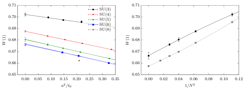
Figure 5: Left: Continuum extrapolation of $W(1)$ for all gauge groups. Right: Large $N$ extrapolations of $W(1)$ in the continuum (solid line) and at finite lattice spacing (dotted line). There is an excellent agreement between the data and the expected scaling in powers of $1/N^{2}$. The points at finite lattice spacing have been slightly shifted for better legibility.

Once again, to quantify the magnitude of the finite $N$ corrections, we collect in Table 2 the values of $a_{1}$ and $a_{2}$ from the fit to $Y$. We observe that the relative magnitude of them grow at larger values of $c$ (or $t$ equivalently). Similarly, the deviation between $\mathrm{SU}(3)$ and $\mathrm{SU}(\infty)$ also grows up to a value of $\eta(1/9)=0.1$ when $c=9/4$. In all cases we find an excellent fit to $Y$ (the values of $\chi^{2}/\mathrm{dof}$ are reported in Table 2).

5.2 Factorization

In order to verify the property of factorization from Eq. (1.1), we take the large $N$ limit of the observables defined in Sec. 2.3. The large $N$ limits are taken in a similar way as described earlier, but we modify the parametrization of the large $N$ fitting function for convenience, so that

$$Y(1/N^{2})=b_{0}+\frac{b_{1}}{N^{2}}+\frac{b_{2}}{N^{4}}\,.$$ (5.27)

For the continuum limit extrapolations we use the same strategy as for $W$ and for $\bar{\lambda}_{\mathrm{GF}}$, and in all cases, the data can be fitted very well with a linear or quadratic polynomial in $a^{2}/t_{0}$. We also check for effects caused by variations of $L/\sqrt{8t}$ in all observables. As discussed in Appendix A, we find that $H_{W}$ at $c=1/2$ and $c=1$, are potentially affected by large effects. We tried to include them as a systematic error on the measurements, but this yields errors which are too large to be of interest as a test of factorization. Hence, we present only results for $H_{W}$ at $c=9/4$ .

Let us first discuss our results for $H_{E}(1)$. On the right panel of Figure 6 we show the large $N$ fits both in the continuum and at a finite lattice spacing. The fits are excellent, which provides yet again confirmation of the scaling in powers of $1/N^{2}$. It is worth mentioning that at finite lattice spacing, where results are very precise, we find that a quadratic fit in $1/N^{2}$, excluding the $\mathrm{SU}(3)$ point, extrapolates to $\mathrm{SU}(3)$ within one standard deviation. In this sense, $\mathrm{SU}(3)$ can be used as validation of our fitting strategy. The values of the parameters of the fitting function $Y$ are displayed in Table 3. At finite lattice spacing we include also the parameters from the fit excluding $\mathrm{SU}(3)$.

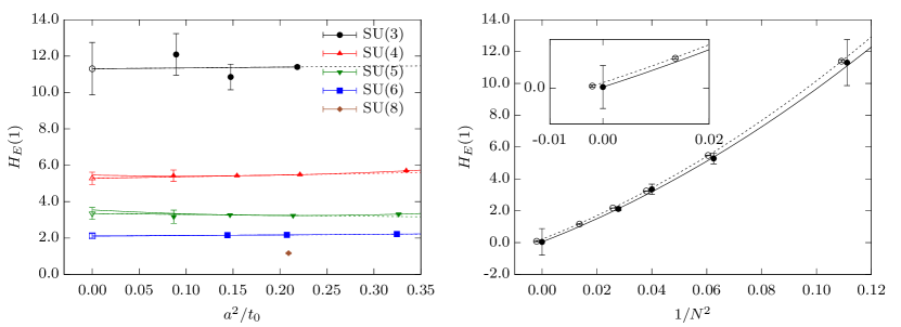
Figure 6: Left: Continuum extrapolation of $H_{E}(1)$ for all gauge groups. Right: Large $N$ extrapolations of $H_{E}(1)$ in the continuum (solid line) and at finite lattice spacing (dotted line). The points at finite lattice spacing have been slightly shifted for better legibility.

obs.	fit	$b_{0}$	$b_{1}$	$b_{2}$	$\chi^{2}/\mathrm{dof}$
$H_{E}(1)$	L	$0.078(44)$	$66.3(19)$	$319(19)$	$0.30$
$H_{E}(1)$	L4	$0.069(75)$	$66.8(35)$	$314(43)$	$0.59$
$H_{E}(1)$	C	$0.04(84)$	$67(39)$	$293(373)$	$0.34$
$H_{E}(1)$	L*	$0.0$	$70.22(60)$	$276(12)$	$0.71$
$H_{E}(1)$	C*	$0.0$	$70.3(98)$	$237(200)$	$0.27$
$G_{W}(1)$	L	$-0.00029(34)$	$0.548(13)$	$-0.69(12)$	$0.02$
$G_{W}(1)$	L4	$-0.00017(69)$	$0.540(44)$	$-0.59(54)$	$<0.01$
$G_{W}(1)$	C	$-0.00003(36)$	$0.49(13)$	$-0.48(86)$	$<0.01$
$G_{W}(1)$	L*	$0.0$	$0.5376(58)$	$-0.619(76)$	$0.25$
$G_{W}(1)$	C*	$0.0$	$0.485(28)$	$-0.48(27)$	$<0.01$
$G_{W}(1/2)$	L	$0.000045(373)$	$0.167(17)$	$-0.17(15)$	$<0.01$
$G_{W}(1/2)$	L4	$-0.000008(646)$	$0.170(42)$	$-0.23(55)$	$<0.01$
$G_{W}(1/2)$	C	$-0.00049(247)$	$0.168(82)$	$-0.32(56)$	$<0.01$
$G_{W}(1/2)$	L*	$0.0$	$0.1686(70)$	$-0.188(90)$	$<0.01$
$G_{W}(1/2)$	C*	$0.0$	$0.152(19)$	$-0.22(18)$	$0.02$
$G_{W}(9/4)$	L	$-0.00124(63)$	$2.781(38)$	$-3.95(43)$	$0.13$
$G_{W}(9/4)$	L4	$-0.0010(10)$	$2.760(74)$	$-3.6(10)$	$0.15$
$G_{W}(9/4)$	C	$0.0014(99)$	$2.43(40)$	$-1.8(29)$	$0.13$
$G_{W}(9/4)$	L*	$0.0$	$2.711(14)$	$-3.23(24)$	$1.39$
$G_{W}(9/4)$	C*	$0.0$	$2.485(73)$	$-2.22(81)$	$0.07$
$H_{W}(9/4)$	L	$-0.24(14)$	$120(9)$	$-129(84)$	$0.39$
$H_{W}(9/4)$	C	$-3.3(25)$	$226(88)$	$-1063(618)$	$0.26$
$H_{W}(9/4)$	L*	$0.0$	$106(3)$	$-7(40)$	$1.17$
$H_{W}(9/4)$	C*	$0.0$	$112(17)$	$-290(186)$	$0.99$

Table 3: Parameters of the large $N$ extrapolations of $H_{E}$, $G_{W}$ and $H_{W}$. We present the results for three different cases, L: at finite lattice spacing, L₄: at finite lattice spacing excluding $\mathrm{SU}(3)$, and C: in the continuum. Additionally, we fit the data to a function with $b_{0}=0$, so that factorization is imposed at finite lattice spacing L* and in the continuum C*. In this case, the value of $\chi^{2}/\mathrm{dof}$ validates this hypothesis.

Concerning the $N\to\infty$ limit itself, the extrapolated value is within two standard deviations from zero in the worst case. Notice that at finite lattice spacing, the errors in the extrapolation are two orders of magnitude smaller than the value of $H_{E}(1)$ at $N=3$. To further validate factorization, an additional fit is performed for which $b_{0}=0$ is fixed, and only $b_{1}$ and $b_{2}$ are fitted to the data. This enforces factorization, so the value of $\chi^{2}/\mathrm{dof}$ from the fit can be used to asses the validity of the assumption ($L^{*},C^{*}$ in Table 3). To summarize, for $H_{E}(1)$ we find excellent agreement with factorization in the continuum, and a deviation compatible with two standard deviations in the worst case at finite lattice spacing, still statistically consistent with factorization.

We now turn to the smooth Wilson loops. In Figure 7 we display the results of the continuum and large $N$ fits for $G_{W}(1)$. The parameters of the extrapolations at the three values of $c$ are displayed in Table 3. Also in this case, we find that $\mathrm{SU}(3)$ can be used as a validation point, and if it is excluded from the fit, it agrees with the extrapolating function within two standard deviations at $c=1$, and within one standard deviation at the remaining values of $c$.

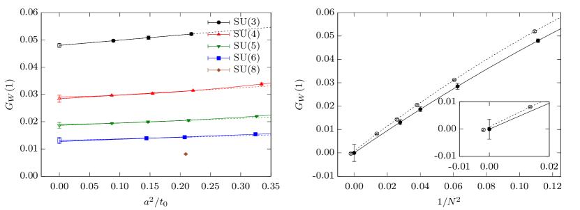
Figure 7: Left: Continuum extrapolation of $G_{W}(1)$ for all gauge groups. Right: Large $N$ extrapolations of $G_{W}(1)$ in the continuum (solid line) and at finite lattice spacing (dotted line). The points at finite lattice spacing have been slightly shifted for better legibility.

For the fits with factorization enforced by fixing $b_{0}=0$, the values of $\chi^{2}/\mathrm{dof}$ are also excellent. These values, together with those of $b_{0}$ reported in Table 3, give us confidence on the validity of factorization. Notice that the errors at large $N$ are at least one order of magnitude smaller than the value at $\mathrm{SU}(3)$ itself. Concerning the finite $N$ corrections, comparing the loops at different values of $c$, we observe that those at large $c$ are characterized by large coefficients in front of the $1/N^{2}$ and $1/N^{4}$ correction terms.

Yet another interesting question is whether loops at fixed $t$ but different $R$ have different finite $N$ corrections. We explore this issue at the end of the section. Let us first look at $H_{W}$ in Figure 8. The $N\to\infty$ limits are less than two standard deviations away from zero. Inspecting the continuum limit fits, we observe that had we taken the three-point extrapolation for $N=6$ as our central result, the central value would have been close to the upper end of the error bar in Figure 8 and the $1/N^{2}$ extrapolation in full agreement with factorization. In other words, one should not look too much at the central value but at the full range of the error, as always.

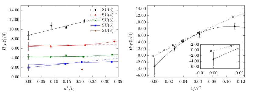
Figure 8: Left: Continuum extrapolation of $H_{W}(9/4)$ for all gauge groups. Right: Large $N$ extrapolations of $H_{W}(9/4)$ in the continuum (solid line) and at finite lattice spacing (dotted line). The points at finite lattice spacing have been slightly shifted for better legibility.

5.2.1 Loop size dependence

$\xi$	$a_{0}$	$a_{1}$	$a_{2}$	$b_{0}$	$b_{1}$	$b_{2}$
$1.00$	$0.7760(7)$	$0.36(3)$	$-0.09(24)$	$0.00005(37)$	$0.167(17)$	$-0.17(15)$
$1.25$	$0.5956(7)$	$0.68(4)$	$0.40(34)$	$0.0003(13)$	$0.752(55)$	$-1.13(44)$
$1.50$	$0.4087(5)$	$1.16(5)$	$1.34(48)$	$0.0005(31)$	$2.62(12)$	$-5.05(92)$
$1.75$	$0.2512(4)$	$1.78(7)$	$3.16(71)$	$0.0053(65)$	$8.06(22)$	$-18.7(17)$
$2.00$	$0.1390(3)$	$2.48(13)$	$6.7(12)$	$0.030(13)$	$26.12(50)$	$-81.0(45)$

Table 4: Parameters of the large $N$ extrapolation of $\hat{W}$ and $\hat{G}_{W}$ as a function of $\xi$.

Finally, let us explore how the finite $N$ corrections to factorization change when the size of the loop is increased at a fixed value of the smoothing parameter $t$. For a given value of $t$, we consider square loops of size $R(\xi)=\xi\sqrt{8t}$. Given the finite size of the lattices, we use the loops measured at $c=1/2$ ($t=t_{0}/2$), so that we can consider larger values of $\xi$. Thus, at a fixed value of $t=t_{0}/2$, we define $\hat{W}$ and $\hat{G}_{W}$ in a similar way as $W$ and $G_{W}$, but in this case, as a function of $\xi$ instead of $c$. In addition to the already presented results at $\xi=1$, we also measured $\hat{W}$ and $\hat{G}_{W}$ at $\xi=1.25,\,1.5,\,1.75$ and $2$. The coefficients obtained for the large $N$ fits at finite lattice spacing are displayed in Table 4 as a function of $\xi$.

Figure 9: Plot of the parameters $a_{1}$ and $\log(b_{1})$ as a function of $\xi$. The interpolating function is a quadratic function in $\xi$ in both cases.

We observe that in the case of the loops themselves, the coefficients of the $1/N^{2}$ expansion do not change significantly with $\xi$, while those of $\hat{G}_{W}$ grow rapidly for larger loops. In fact, they grow exponentially fast as shown in Figure 9. At finite $N$, larger loops are much further away from $N\to\infty$ than smaller loops.

6 Conclusions

We have taken the large $N$ limit of a few observable of $\mathrm{SU}(N)$ pure gauge theories numerically defining all dimensionfull quantities in units of $t_{0}$. This means that we held $t_{0}$, or equivalently the coupling $\bar{\lambda}_{\mathrm{GF}}$, eq. (2.6), at a low energy fixed in defining the approach to the limit. As explained in Sect. 3, the precise magnitude of $1/N^{2}$ corrections do depend on this choice. For each quantity, the continuum limit was taken before the large $N$ limit, but we have also investigated large $N$ scaling at finite lattice spacing, defined by $a^{2}/t_{0}$=constant.

In both cases we find that finite $N$ observables are very well and very precisely described by a leading order term and corrections $\sim 1/N^{2}$ and $\sim 1/N^{4}$. We recall for example Figure 4 where the excellent precision, in particular at finite $a$, is visible. In the same way, factorization has been confirmed very precisely. Of course, a numerical computation cannot substitute a mathematical proof, but our results make it very implausible that anything goes wrong with the large $N$ limit in general, or factorization in particular.

However, the magnitude of corrections to the large $N$ limit is more complex. We found a strong dependence on the physical size of the observables. For example, we considered $R\times R$ Wilson loops smoothed with a smoothing radius of size again $\sqrt{8t}=R$. Table 2 shows the deviation, $\eta$, of SU(3) from SU($\infty$) of these smooth loops to increase from 3% at a loop-size of $r=0.2\,\mathrm{fm}$ to 10% at $R=1\,\mathrm{fm}$.

When we increase the loop size $R$ at fixed smoothing radius $\sqrt{8t}=0.23\,\mathrm{fm}$ from $R=0.23\,\mathrm{fm}$ to $R=0.5\,\mathrm{fm}$, the corrections $\eta(1/9)\approx a_{1}/9$ (with $a_{1}$ from Table 4 or Figure 9) grow from 4% to more than 30%. The growth with $R$ of the finite $N$ corrections to factorization is even more dramatic as seen on the right panel in Figure 9. These large corrections may also contribute to the fact that one has to go to very large $N$ to approach the large $N$ limit in the 1-point model [8, 52]. Of course, the dominating effect is expected to be that the color degrees of freedom provide the effective size of the system in that model.

In summary, large $N$ scaling is confirmed with high precision, but corrections to large distance observables can be substantial. One thus has to be careful when deriving quantitative information from large $N$ considerations in gauge theories.

Acknowledgements.  We would like to thank M. Cè, L. Giusti and S. Schaefer for sharing part of the generation of the gauge configurations [2] and M. Koren for useful discussions. We are grateful to A. Gonzalez-Arroyo and U. Wolff for their valuable comments on our first manuscript. Our simulations were performed at the ZIB computer center with the computer resources granted by The North-German Supercomputing Alliance (HLRN). M.G.V acknowledges the support from the Research Training Group GRK1504/2 “Mass, Spectrum, Symmetry” founded by the German Research Foundation (DFG).

Appendix A Volume dependence

In order to understand whether $L$ is kept sufficiently close to a fixed value, we have performed two additional simulations at the coarsest lattice spacing for $\mathrm{SU}(4)$ and $\mathrm{SU}(5)$. The parameters for these simulations are the same as for $A(4)_{1}$ and $A(5)_{1}$ respectively, with the difference that the lattice sizes have been increased to $24^{3}\times 96$. In physical units this corresponds to $L\approx 2.4\,\mathrm{fm}$. Although all the ensembles in Table 1 have approximately the same lattice size, we find that in the case of $H_{W}(c)$, at $c=1/2$ and $c=1$, the small variations in the volume induces an uncertainty which may be relevant. For the rest of observables, volume effects are within the statistical uncertainty. To showcase this, in Figure 10 we display a plot of $H_{W}(c)$ for $c=1/2$ and $c=9/4$. Clearly, at the smaller $c$, volume effects are much larger. Both at $c=1/2$ and $c=1$ we find that including the volume effects as a systematic correction is difficult with just two points in $L$. Attempting it in a conservative manner produces errors which are too large to check for the large $N$ scaling at a similar precision as for the rest of observables, so we include only $H_{W}(9/4)$ in the analysis. We note that we do not have an explanation why small $c$ appears to be more difficult than a large one.

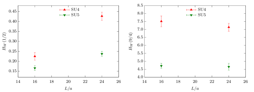
Figure 10: Finite volume checks for $H_{W}$. On the left at $c=1/2$, and on the right at $c=9/4$. Notice that at the smaller $c$ the finite volume corrections are very significant.

Appendix B $\bar{\lambda}_{\mathrm{GF}}$ at small $t$

As stressed in Sec. 5.1.1, the continuum extrapolations become more difficult at smaller values of $t$. Due to the large cut-off effects, we find that a linear extrapolation in $a^{2}/t_{0}$ does not parametrize the data adequately, even using only the finest lattice points. For that reason, we include in the fits the $\mathrm{O}(a^{4}/t_{0}^{2})$ and the $\mathrm{O}(a^{6}/t_{0}^{3})$ corrections. The fit strategy is similar to the one used for the rest observables, except that higher degree polynomials are used. Briefly, the central point is obtained by performing a quadratic fit in $a^{2}/t_{0}$ using those data for which $a^{2}/t_{0}\leq 1/4$. Then, a second fit is performed, either using a quadratic function, or a cubic one if the value of $\chi^{2}/\mathrm{dof}$ of the first one is too large. Finally, the error is chosen so that it covers the full 1-$\sigma$ band of both fits. We show our results at $t/t_{0}=0.2$ in Figure 11. As expected, the errors in our continuum extrapolations are larger than those obtained at larger values of $t$, but within the errors, the large $N$ extrapolation is perfectly consistent with a polynomial in $1/N^{2}$. At finite lattice spacing, the large $N$ extrapolation is cleaner, and once again it shows and excellent agreement with the ’t Hooft expansion.

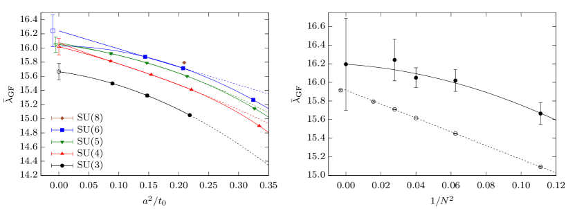
Figure 11: Left: Continuum extrapolation of $\bar{\lambda}_{\mathrm{GF}}$ at $t/t_{0}=0.2$ for all the different gauge groups. Right: Large $N$ extrapolations of $\bar{\lambda}_{\mathrm{GF}}$ in the continuum (solid line) and at finite lattice spacing (dotted line). There is an excellent agreement between the data and the expected scaling in powers of $1/N^{2}$. The points at finite lattice spacing have been slightly shifted for better legibility.

References

- [1] G. ’t Hooft, A Planar Diagram Theory for Strong Interactions, Nucl. Phys. B72 (1974) 461.
- [2] M. Cè, M. García Vera, L. Giusti, and S. Schaefer, The topological susceptibility in the large- N limit of SU( N ) Yang–Mills theory, Phys. Lett. B762 (2016) 232–236, [arXiv:1607.0593].
- [3] A. Donini, P. Hernández, C. Pena, and F. Romero-López, Nonleptonic kaon decays at large , Phys. Rev. D94 (2016), no. 11 114511, [arXiv:1607.0326].
- [4] T. DeGrand and Y. Liu, Lattice study of large QCD, Phys. Rev. D94 (2016), no. 3 034506, [arXiv:1606.0127]. [Erratum: Phys. Rev.D95,no.1,019902(2017)].
- [5] B. Lucini, M. Teper, and U. Wenger, Glueballs and k-strings in SU(N) gauge theories: Calculations with improved operators, JHEP 06 (2004) 012, [hep-lat/0404008].
- [6] A. Gonzalez-Arroyo and M. Okawa, The string tension from smeared Wilson loops at large N, Phys. Lett. B718 (2013) 1524–1528, [arXiv:1206.0049].
- [7] B. Lucini, A. Rago, and E. Rinaldi, SU() gauge theories at deconfinement, Phys. Lett. B712 (2012) 279–283, [arXiv:1202.6684].
- [8] A. Gonzalez-Arroyo and M. Okawa, Testing volume independence of SU(N) pure gauge theories at large N, JHEP 12 (2014) 106, [arXiv:1410.6405].
- [9] M. J. Teper, SU(N) gauge theories in (2+1)-dimensions, Phys. Rev. D59 (1999) 014512, [hep-lat/9804008].
- [10] B. Lucini and M. Teper, SU(N) gauge theories in (2+1)-dimensions: Further results, Phys. Rev. D66 (2002) 097502, [hep-lat/0206027].
- [11] B. Bringoltz and M. Teper, A Precise calculation of the fundamental string tension in SU(N) gauge theories in 2+1 dimensions, Phys. Lett. B645 (2007) 383–388, [hep-th/0611286].
- [12] J. Liddle and M. Teper, The Deconfining phase transition in D=2+1 SU(N) gauge theories, arXiv:0803.2128.
- [13] A. Athenodorou and M. Teper, SU(N) gauge theories in 2+1 dimensions: glueball spectra and k-string tensions, JHEP 02 (2017) 015, [arXiv:1609.0387].
- [14] L. G. Yaffe, Large n Limits as Classical Mechanics, Rev. Mod. Phys. 54 (1982) 407.
- [15] E. Witten, THE 1 / N EXPANSION IN ATOMIC AND PARTICLE PHYSICS, NATO Sci. Ser. B 59 (1980) 403–419.
- [16] S. R. Coleman, 1/N, in 17th International School of Subnuclear Physics: Pointlike Structures Inside and Outside Hadrons Erice, Italy, July 31-August 10, 1979, p. 0011, 1980.
- [17] P. Rossi, M. Campostrini, and E. Vicari, The Large N expansion of unitary matrix models, Phys. Rept. 302 (1998) 143–209, [hep-lat/9609003].
- [18] P. D. Vecchia, R. Musto, F. Nicodemi, R. Pettorino, and P. Rossi, The transition from the lattice to the continuum: models at large n, Nuclear Physics B 235 (1984), no. 4 478 – 520.
- [19] M. Campostrini and P. Rossi, The 1/N expansion of two-dimensional spin models, Riv. Nuovo Cim. 16 (1993), no. 6 1–111.
- [20] M. Campostrini and P. Rossi, The 1/N expansion of two-dimensional spin models, Nucl. Phys. Proc. Suppl. 34 (1994) 680–682, [hep-lat/9305007].
- [21] T. Eguchi and H. Kawai, Reduction of Dynamical Degrees of Freedom in the Large N Gauge Theory, Phys.Rev.Lett. 48 (1982) 1063.
- [22] J. Kiskis, R. Narayanan, and H. Neuberger, Does the crossover from perturbative to nonperturbative physics in QCD become a phase transition at infinite N?, Phys. Lett. B574 (2003) 65–74, [hep-lat/0308033].
- [23] A. Gonzalez-Arroyo and M. Okawa, The Twisted Eguchi-Kawai Model: A Reduced Model for Large N Lattice Gauge Theory, Phys. Rev. D27 (1983) 2397.
- [24] A. Gonzalez-Arroyo and M. Okawa, A Twisted Model for Large Lattice Gauge Theory, Phys. Lett. B120 (1983) 174–178.
- [25] A. Gonzalez-Arroyo and M. Okawa, Large reduction with the Twisted Eguchi-Kawai model, JHEP 07 (2010) 043, [arXiv:1005.1981].
- [26] Yu. M. Makeenko and A. A. Migdal, Exact Equation for the Loop Average in Multicolor QCD, Phys. Lett. B88 (1979) 135. [Erratum: Phys. Lett.B89,437(1980)].
- [27] A. Chatterjee and D. Gangopadhyay, FACTORIZATION IN LARGE N LIMIT OF LATTICE GAUGE THEORIES REVISITED, Pramana 21 (1983) 385–391.
- [28] Y. Makeenko, Large N gauge theories, hep-th/0001047.
- [29] S. Chatterjee, Rigorous solution of strongly coupled lattice gauge theory in the large limit, arXiv:1502.0771.
- [30] J. Jafarov, Wilson loop expectations in lattice gauge theory, arXiv:1610.0382.
- [31] M. Lüscher and P. Weisz, Perturbative analysis of the gradient flow in non-abelian gauge theories, JHEP 02 (2011) 051, [arXiv:1101.0963].
- [32] V. S. Dotsenko and S. N. Vergeles, Renormalizability of Phase Factors in the Nonabelian Gauge Theory, Nucl. Phys. B169 (1980) 527–546.
- [33] R. A. Brandt, F. Neri, and M.-a. Sato, Renormalization of Loop Functions for All Loops, Phys. Rev. D24 (1981) 879.
- [34] H. Dorn, Renormalization of Path Ordered Phase Factors and Related Hadron Operators in Gauge Field Theories, Fortsch. Phys. 34 (1986) 11–56.
- [35] M. Creutz, Monte Carlo Study of Renormalization in Lattice Gauge Theory, Phys. Rev. D23 (1981) 1815.
- [36] R. Narayanan and H. Neuberger, Infinite N phase transitions in continuum Wilson loop operators, JHEP 03 (2006) 064, [hep-th/0601210].
- [37] M. Lüscher, Properties and uses of the Wilson flow in lattice QCD, JHEP 08 (2010) 071, [arXiv:1006.4518]. [Erratum: JHEP03,092(2014)].
- [38] M. Okawa and A. Gonzalez-Arroyo, String tension from smearing and Wilson flow methods, PoS LATTICE2014 (2014) 327, [arXiv:1410.7862].
- [39] R. Lohmayer and H. Neuberger, Rectangular Wilson Loops at Large N, JHEP 08 (2012) 102, [arXiv:1206.4015].
- [40] R. Lohmayer and H. Neuberger, Non-analyticity in scale in the planar limit of QCD, Phys. Rev. Lett. 108 (2012) 061602, [arXiv:1109.6683].
- [41] B. Alles, A. Feo, and H. Panagopoulos, The Three loop Beta function in SU(N) lattice gauge theories, Nucl. Phys. B491 (1997) 498–512, [hep-lat/9609025].
- [42] R. F. Dashen and D. J. Gross, The Relationship Between Lattice and Continuum Definitions of the Gauge Theory Coupling, Phys. Rev. D23 (1981) 2340. [,246(1980)].
- [43] G. ’t Hooft, Large N, in Phenomenology of large N(c) QCD. Proceedings, Tempe, USA, January 9-11, 2002, pp. 3–18, 2002. hep-th/0204069.
- [44] M. Lüscher and S. Schaefer, Lattice QCD without topology barriers, JHEP 07 (2011) 036, [arXiv:1105.4749].
- [45] N. Cabibbo and E. Marinari, A New Method for Updating SU(N) Matrices in Computer Simulations of Gauge Theories, Phys. Lett. B119 (1982) 387–390.
- [46] M. Cè, C. Consonni, G. P. Engel, and L. Giusti, Non-Gaussianities in the topological charge distribution of the SU(3) Yang–Mills theory, Phys. Rev. D92 (2015), no. 7 074502, [arXiv:1506.0605].
- [47] R. Sommer, A New way to set the energy scale in lattice gauge theories and its applications to the static force and alpha-s in SU(2) Yang-Mills theory, Nucl. Phys. B411 (1994) 839–854, [hep-lat/9310022].
- [48] M. García Vera and S. Schaefer, Multilevel algorithm for flow observables in gauge theories, Phys. Rev. D93 (2016) 074502, [arXiv:1601.0715].
- [49] M. G. Vera and R. Sommer, Large scaling and factorization in Yang-Mills theory, EPJ Web Conf. 175 (2018) 11018, [arXiv:1710.0605].
- [50] M. Cè, M. García Vera, L. Giusti, and S. Schaefer, The large limit of the topological susceptibility of Yang-Mills gauge theory, PoS LATTICE2016 (2016) 350, [arXiv:1610.0879].
- [51] ALPHA Collaboration, M. Dalla Brida, P. Fritzsch, T. Korzec, A. Ramos, S. Sint, and R. Sommer, Slow running of the Gradient Flow coupling from 200 MeV to 4 GeV in QCD, Phys. Rev. D95 (2017), no. 1 014507, [arXiv:1607.0642].
- [52] A. González-Arroyo and M. Okawa, Large N meson masses from a matrix model, Phys. Lett. B755 (2016) 132–137, [arXiv:1510.0542].